1 Basic Concepts of Thermodynamics and Statistical Physics

1

Basic Concepts of Thermodynamicsand Statistical Physics

Summary. The basic concepts and postulates of thermodynamics and statisti-cal physics are expounded in this chapter. Different ways of description of thestate of macroscopic systems, consisting of a very large number of particles suchas atoms, molecules, ions, electrons, photons, phonons, etc., are adduced. Suchconcepts as the distribution function over microstates, statistical weight of the pre-assigned macroscopic state of a system, absolute temperature, and pressure are alsointroduced.

1.1 Macroscopic Description of State of Systems:Postulates of Thermodynamics

As noted in the Foreword, thermodynamics and statistical physics study phys-ical properties of macroscopic systems with a large number of degrees offreedom. The lifetime of these systems ought to be sufficiently long to con-duct experiments on them. A usual gas, consisting of atoms or molecules,photon gas, plasma, liquid, crystal, and so on, can serve as an example ofsuch systems. A small but macroscopic part of the considered system is calleda subsystem.

Macroscopic systems can interact between themselves or with the sur-rounding medium by the following channels:

1. An interaction when the considered system performs work on other sys-tems, or vice versa, is called mechanical interaction (ΔA �= 0). In thiscase, the volume of the system changes.

2. An interaction in which the energy of the system changes only at theexpense of heat transfer (without performing work) is called thermalinteraction (ΔQ �= 0).

3. An interaction leading to exchange of particles between systems or betweenthe system and the surrounding medium is called material interaction(ΔN �= 0).

2 1 Basic Concepts of Thermodynamics and Statistical Physics

Depending on which of the above-indicated channels is open or closed, differenttypes of macroscopic systems exist in nature.

A system is called isolated if energy and material exchange with the sur-rounding medium is absent (ΔA = 0, ΔQ = 0, ΔN = 0). For such systemsall channels of interaction are closed.

If a system is surrounded by a heat-insulated shell, the system is called anadiabatically isolated system (ΔQ = 0).

If a system does not exchange particles with the surrounding medium(ΔN = 0), such a system is called closed, and, on the other hand, if exchangeof particles (ΔN �= 0) takes place, the system is called open.

If the considered system is a small but macroscopic part of a large system,physical processes occurring in it will hardly influence the thermodynamicstate of the large system. In this case, the large system is called a thermostat,and the system interacting with it is a system in the thermostat.

The thermodynamic state of each system at pre-assigned external condi-tions can be described by a restricted number of physical quantities which canbe measured on test. Such quantities are called thermodynamic parameters.The number of particles in a system N , its volume V , pressure P , absolutetemperature T , dielectric P and magnetic M polarization vectors, electricE and magnetic H field strengths are examples of thermodynamic param-eters. These parameters characterize the system itself and also the externalconditions in which it is found.

Parameters that are determined by coordinates of external bodies inter-acting with a system are called external parameters: volume, the electric andthe magnetic field strength, etc. Parameters that, apart from coordinates ofexternal bodies, depend also on coordinates and impulses of particles enter-ing into the system are called internal parameters: pressure, temperature, theinternal energy, dielectric and magnetic polarizations.

Internal parameters can be intensive or extensive. Parameters not depend-ing on the number of particles in a system are called intensive: pressure,temperature, etc. Parameters that are proportional to the number of particlesor the amount of substance are called extensive or additive: entropy, energyand other thermodynamic potentials.

The state of a system determined by the totality of the above-enumerated,measured-on-test thermodynamic parameters is called a macroscopic state ofthe system:

Macroscopic state ⇒ (N, V, P, T, P, M , E,H , . . .) .

It is evident that these macroscopic parameters determine the averaged stateof a system, in that the details and the nature of the complex motion ofparticles composing the system are disregarded. Such a description of a systembears the phenomenological, i.e. the descriptive, character.

If thermodynamic parameters determining the state of a system do notdepend on time, such a state is called stationary. Moreover, if stationary flows

1.1 Macroscopic Description of State of Systems 3

and currents are absent in a system, such a state is called a thermodynamicequilibrium. This state is the simplest macroscopic state of a system. It is tobe noted that even in this state, inside the system particles perform complexchaotic motion; however, this motion is not of interest in thermodynamics.

After introducing the primary basic thermodynamic concepts, we pass onto the exposition of two postulates comprising the basis of thermodynamics.These postulates were established from generalizations of experimental data.

The first postulate of thermodynamics states that each isolated systemhas only one intrinsic state, that of thermodynamic equilibrium. If a systemis not in the equilibrium state, it tends toward its equilibrium state over aperiod of time, and once it has achieved that state, can never come out of itspontaneously without an external force being exerted on it.

Also called the general principle of thermodynamics, this postulate definesthe thermodynamic equilibrium state. This principle is demonstrated by anexample of the macroscopic parameter L (Fig. 1.1). The time τ during whichthe parameter L(t) passes to the equilibrium state L0 is called the relaxationtime. The quantity τ depends on the nature of interaction and intensity ofthe motion of the particles composing the system.

The first postulate of thermodynamics determines the limit of applicabil-ity of the laws of thermodynamics. Indeed, inasmuch as each system consistsof chaotically moving particles, the parameter L(t) can deviate from its meanvalue, i.e. a fluctuation occurs. These deviations are schematically shown inFig. 1.1. Thermodynamics disregards these fluctuations and takes only themean values measured on test into consideration. Therefore the laws of ther-modynamics are applicable only to systems in which deviations from the meanvalues are much smaller than the mean values themselves. But this is possibleonly in systems with a sufficiently large number of particles.

If a system consists of a small number of particles, the relative fluctuationcan be large and the system itself can move away from the equilibrium state.In this case, the concept of “the equilibrium state” loses its sense, and thefirst postulate of thermodynamics is violated. It can be demonstrated by asimple example. Let us assume that a gas contained in a rectangular vesselcontains N particles. Mentally divide the vessel into two equal parts. In theequilibrium state, in each half N/2 molecules ought to be found. If N = 4,

τ t0

L (t)

L0

Fig. 1.1. The fluctuation of the thermodynamical parameter


often the following picture can be observed: in the first part there are threemolecules, and in the second there is one molecule; or, in the first part thereare four molecules, and the second part is empty. Such a situation means thatthe system itself is not in the equilibrium state, in which N/2 = 2 moleculesshould be present in each part of the vessel.

Thus, from the first postulate the following conclusion can be made: Lawsof thermodynamics are not applicable to systems consisting of a small numberof particles.

The second postulate of thermodynamics states that if two systems A andB are separately found in thermodynamic equilibrium with the third system C,A and B are also found in thermodynamic equilibrium between themselves, i.e.

A ∼ CB ∼ C

}⇒ A ∼ B. (1.1)

This postulate is also called the zeroth law of thermodynamics and, as we willsee below, defines the concept of absolute temperature.

The second postulate determines the upper boundary of applicability ofthe laws of thermodynamics. As seen from this postulate, when bringing intothermal contact subsystems A, B, C, or while disconnecting them, the stateof equilibrium is not violated, i.e. the energy of interaction of the subsystemsis negligibly small and the energy of the whole system is an additive quantity1

E =∑

α

Eα, (1.2)

where Eα is the energy of the subsystem α.Thus, the laws of thermodynamics are applicable only to systems for which

the condition of additivity of energy (1.2) is fulfilled. Naturally, the conditionof additivity is not fulfilled for large systems, individual parts of which interactthrough a gravitational field.2 Therefore, the laws of thermodynamics are notapplicable to very large, complex systems, e.g. to the universe as a whole.

From the second postulate, besides the principle of additivity of energy, thesecond, not less important, conclusion stems. Indeed, from this postulate it fol-lows that if A, B, C are subsystems of a large system in the equilibrium state,their state, besides the external parameters, ought to be characterized also bythe general internal parameter. This internal intensive parameter is calledtemperature and is identical in all parts of the large system, which is in thethermodynamic equilibrium state. Temperature is determined by the intensityof the thermal motion of the particles in the system. Thus, according to thesecond postulate, the thermodynamic equilibrium state of a system is deter-mined by the totality of external parameters and temperature. Consequently,1 Equality (1.2) supposes that the energy of interaction between subsystems is

negligible small compared with the internal energy of a subsystem.2 In this case, the gravitational energy of interaction between parts cannot be

neglected.

1.1 Macroscopic Description of State of Systems 5

according to the second postulate, each internal parameter is a function ofexternal parameters and temperature. This conclusion relates any internalparameter Ai to temperature T and external parameters a1, a2, . . . , an:

Ai = Ai(a1, a2, . . . , an;T ); i = 1, 2, . . . κ, (1.3)

where k is the number of internal parameters. This equation, written in thesymbolic form, is called the equation of state. The number of such equations,naturally, equals the number of internal parameters k.

If in the capacity of an internal parameter we accept the internal energyof a system Ai ≡ E, (1.3) can be presented in the form:

E = E(a1, a2, . . . , an;T ). (1.4)

This equation is called the caloric equation of the state of a system.If in the capacity of an internal parameter we accept pressure Ai ≡ P ,

from (1.3) we get the thermal equation of state:

P = P (a1, a2, . . . , an;T ). (1.5)

Thus, from the set of equations (1.3) it is seen that the thermodynamicstate of a system is single-valuedly determined by (n+1) independent numberof parameters. Therefore, the number (n + 1) is called the thermodynamicdegree of freedom of a system. Depending on the complexity of a system, ntakes on values n = 1, 2, 3, . . ..

In the simplest case of closed systems,3 if in the capacity of an independentexternal parameter volume V is accepted, the internal parameter pressure Pand internal energy E, conforming to (1.3), can be expressed as follows:

P = P (V ;T ); E = E(V ;T ). (1.6)

The explicit form of these equations for ideal gases is experimentally deter-mined and theoretically substantiated by statistical methods:

P =N

Vk0T ; E =

32k0TN , (1.7)

where N is the number of particles of an ideal gas, and k0 is the Boltzmannconstant.

If from (1.4) we determine temperature and substitute it into (1.3),all internal parameters can be expressed by E and external parametersa1, a2, . . . , an. Thus, the second postulate of thermodynamics can be alsoexpressed as follows: All internal parameters of a system found in thermo-dynamic equilibrium are functions of external parameters and energy:

Ai = Ai(a1, a2, . . . , an;E). (1.8)3 A gas consisting of the pre-assigned number of neutral atoms or molecules can be

considered as an example.


Systems satisfying this condition are called ergodic. Consequently, thermody-namics is applicable only to ergodic systems.

For an ideal gas, using (1.7), the equation of type (1.8) takes the followingexplicit form:

P =23E

V. (1.9)

Finally, note once more that the first postulate of thermodynamics defines theconcept of thermodynamic equilibrium and the second one defines the conceptof absolute temperature.

1.2 Mechanical Description of Systems:Microscopic State: Phase Space: Quantum States

It is known that any macroscopic system consists of a colossal but finitenumber of particles, and also that each particle can have a complex inter-nal structure. Here the structure of a particles does not interest us, and wewill regard that the considered system as consisting of N number of chaoti-cally moving material points interacting among themselves. Thus, the numberof degrees of freedom of the considered system is 3N . Note that under normalconditions 1 cm3 of air contains 3 × 1019 molecules. The linear dimension ofeach molecule is 10−8 cm. In order to have a notion of the number of parti-cles and their dimensions, we quote a known example by Kelvin, accordingto which the number of H2O molecules in a glass of water is 100 times thenumber of glasses of water available in all oceans and seas of the world.

Naturally, it is impossible to describe in detail the state of such a macro-scopic system with a small number of thermodynamic parameters, since theseparameters disregard the internal structure of the system. For the completedescription of a system, it is necessary to know which particles it consistsof, what nature of their interaction is and by which equations their motionis described, i.e. whether the motion of particles obeys classical or quantummechanical laws. In conformity with this, in nature two types of systems exist:classical and quantum systems. We consider these cases separately.

Classical systems. The motion of particles forming such systems obeysthe laws of classical mechanics, and the state of each of them is determinedby three generalized coordinates qi(t) and by three corresponding generalizedimpulses pi(t),4 where i takes on the value i=1, 2, 3. Consequently, the generalstate of a classical system consisting of N particles at the instant of time t isdetermined by 6N quantities:

microstate ⇒ (q, p) ≡ (q1, q2, . . . , q3N ; p1, p2, . . . , p3N ). (1.10)

4 In classical statistical physics the motion of particles is characterized not by veloc-ity, but by impulse, as the Liouville theorem (Sect. 1.3) is just not in the spaceof coordinates and velocity (q, q), but in the phase space (q, p).

1.2 Mechanical Description of Systems 7

The state of a system being determined by 3N generalized coordinates and 3Ngeneralized impulses is called the microscopic state or, briefly, the microstateof the classical system. The quantities qi(t) and pi(t), i.e. the microstates ofthe system, are found from a solution of the system of Hamilton canonicalequations:

qi =∂H

∂pi, pi = −∂H

∂qi; i = 1, 2, 3, . . . , 3N, (1.11)

where 3N is the number of degrees of freedom of the system, the points overqi and pi mean the time derivative and H is the Hamilton function of thesystem. For conservative systems, H coincides with the total energy E(q, p)of the system:

H ≡ E(q, p) =3N∑i=1

p2i

2m+ U(q1, q2, . . . , q3N ), (1.12)

wherem is the mass of a particle and U(q) is the potential energy of interactionof particles; it is supposed that an external field is absent.

To describe a microstate of classical systems, it is convenient to introducethe concept of phase space or the Γ-space. Each system has its intrinsic phasespace. For instance, the phase space of a classical system consisting of Nparticles represents an abstract 6N -dimensional space. The position of each“point” in this space is determined by 3N generalized coordinates qi and 3Ngeneralized impulses pi, i.e. by 6N quantities.

Thus, a microstate of a classical system consisting of N particles has acorresponding “point” – a phase point – in the 6N -dimensional phase space.

Henceforth, for an elementary volume of the phase space dΓ we will usethe following symbolic notation:

dΓ = dq dp ≡3N∏i=1

dqi dpi. (1.13)

Hence it is seen that the dimensionality of an element of “volume” of the phasespace of a classical system consisting of N particles is (action)3N .

The phase space can be subdivided into two subspaces: coordinates andimpulses. Then, for an element of volume of the phase space one can writedΓ = dΓq · dΓp.

For some systems (e.g. an ideal gas) instead of the Γ-space, we may intro-duce the concept of the μ-space. The μ-space is a six-dimensional space, eachpoint of which is determined by a coordinate and an impulse of one particle(x, y, z, px, py, pz). It is evident that in the μ-space a microstate of an idealgas consisting of N particles is described by a multitude of N points.

Coordinates qi(t) and impulses pi(t) of particles forming a system contin-ually change in conformity with equations of motion (1.11); therefore, themicrostate of the system changes with time. As a result, the position ofphase points changes, describing a specified “curve” in the 6N -dimensional


phase space. This curve is called the phase trajectory.5 The equation of thephase trajectory, in principle, can be found from the solution of the sys-tem of equations (1.11). These solutions can be written symbolically in thefollowing form:{

qi = qi(t; q01, q02, . . . , q03N ; p01, p02, . . . , p03N )pi = pi(t; q01, q02, . . . , q03N ; p01, p02, . . . , p03N), (1.14)

where q0i and p0i are initial coordinates and impulses, respectively, of aparticle.

Note that the phase trajectory can be closed, but it cannot intersect ortouch itself. This result follows from the principle of determinism of classicalmechanics, i.e. the single-valuedness of the solution (1.14) of the equation ofmotion (1.11).6

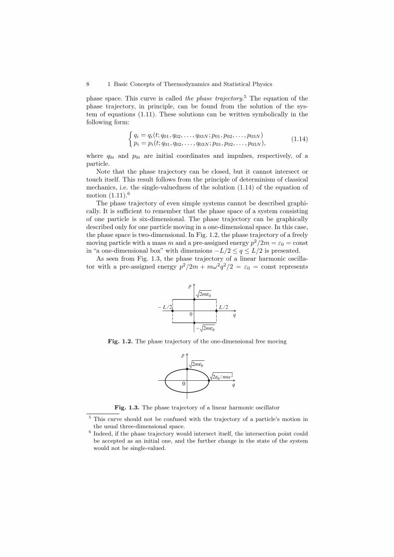
The phase trajectory of even simple systems cannot be described graphi-cally. It is sufficient to remember that the phase space of a system consistingof one particle is six-dimensional. The phase trajectory can be graphicallydescribed only for one particle moving in a one-dimensional space. In this case,the phase space is two-dimensional. In Fig. 1.2, the phase trajectory of a freelymoving particle with a mass m and a pre-assigned energy p2/2m = ε0 = constin “a one-dimensional box” with dimensions −L/2 ≤ q ≤ L/2 is presented.

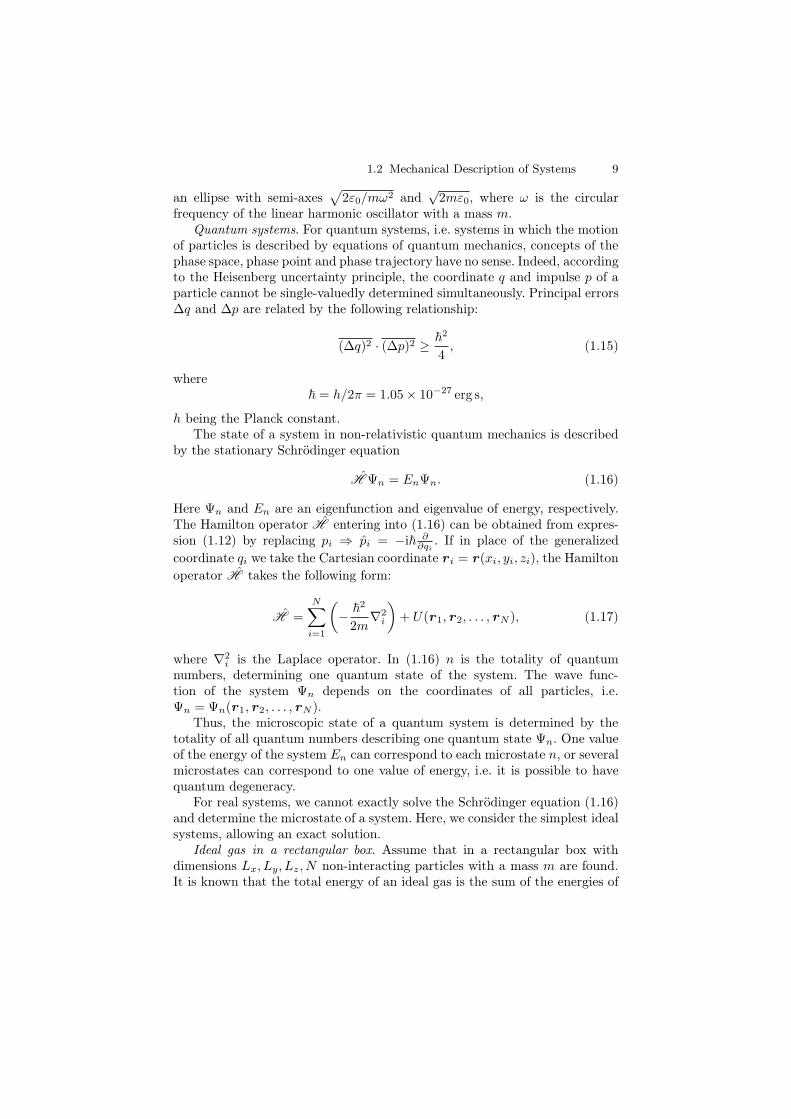
As seen from Fig. 1.3, the phase trajectory of a linear harmonic oscilla-tor with a pre-assigned energy p2/2m + mω2q2/2 = ε0 = const represents

0 q

p

2me0

− 2me0

L /2− L / 2

Fig. 1.2. The phase trajectory of the one-dimensional free moving

0 q

p

2me0

2e0 /mω 2

Fig. 1.3. The phase trajectory of a linear harmonic oscillator5 This curve should not be confused with the trajectory of a particle’s motion in

the usual three-dimensional space.6 Indeed, if the phase trajectory would intersect itself, the intersection point could

be accepted as an initial one, and the further change in the state of the systemwould not be single-valued.


an ellipse with semi-axes√

2ε0/mω2 and√

2mε0, where ω is the circularfrequency of the linear harmonic oscillator with a mass m.

Quantum systems. For quantum systems, i.e. systems in which the motionof particles is described by equations of quantum mechanics, concepts of thephase space, phase point and phase trajectory have no sense. Indeed, accordingto the Heisenberg uncertainty principle, the coordinate q and impulse p of aparticle cannot be single-valuedly determined simultaneously. Principal errorsΔq and Δp are related by the following relationship:

(Δq)2 · (Δp)2 ≥ �2

4, (1.15)

where� = h/2π = 1.05 × 10−27 erg s,

h being the Planck constant.The state of a system in non-relativistic quantum mechanics is described

by the stationary Schrodinger equation

H Ψn = EnΨn. (1.16)

Here Ψn and En are an eigenfunction and eigenvalue of energy, respectively.The Hamilton operator H entering into (1.16) can be obtained from expres-sion (1.12) by replacing pi ⇒ pi = −i� ∂

∂qi. If in place of the generalized

coordinate qi we take the Cartesian coordinate r i = r(xi, yi, zi), the Hamiltonoperator H takes the following form:

H =N∑

i=1

(− �

2

2m∇2

i

)+ U(r1, r2, . . . , rN ), (1.17)

where ∇2i is the Laplace operator. In (1.16) n is the totality of quantum

numbers, determining one quantum state of the system. The wave func-tion of the system Ψn depends on the coordinates of all particles, i.e.Ψn = Ψn(r1, r2, . . . , rN ).

Thus, the microscopic state of a quantum system is determined by thetotality of all quantum numbers describing one quantum state Ψn. One valueof the energy of the system En can correspond to each microstate n, or severalmicrostates can correspond to one value of energy, i.e. it is possible to havequantum degeneracy.

For real systems, we cannot exactly solve the Schrodinger equation (1.16)and determine the microstate of a system. Here, we consider the simplest idealsystems, allowing an exact solution.

Ideal gas in a rectangular box. Assume that in a rectangular box withdimensions Lx, Ly, Lz, N non-interacting particles with a mass m are found.It is known that the total energy of an ideal gas is the sum of the energies of


the individual particles:

En =N∑

i=1

εni , (1.18)

where

εni =�

2

2m(k2ix + k2

iy + k2iz

)(1.19)

is the quantum mechanical energy of the i th particle;

kix =(π

Lx

)nix , kiy =

(π

Ly

)niy , kiz =

(π

Lz

)niz (1.20)

are components of the wave vector, where

nix , niy , niz = 1, 2, 3, . . . (1.21)

are quantum numbers of the ith particle, taking on any positive integer value;and n ⇒ (n1x, n1y, n1z;n2x, n2y, n2z; . . . ;nNx , ;nNy , nNz ) is the totality ofquantum numbers determining the state of a system.

If we substitute the value of the wave vector (1.20) into (1.19), the energyof the ith particle εni can be expressed by the quantum numbers

εni =π2

�2

2m

(n2

ix

L2x

+n2

iy

L2y

+n2

iz

L2z

). (1.22)

As can be seen, the energy of the ith particle of an ideal gas is determinedby three quantum numbers nix , niy , niz (the spin of a particle is disregarded).From quantum mechanics, it is known that in such a case each totality ofquantum numbers has only one corresponding wave function, i.e. one quantumstate, and the degeneracy is absent.

If the energy of a particle (1.22) is taken into account in (1.18), it can besaid that one microstate of an ideal gas in the box is determined by assigning3N quantum numbers, i.e. for the considered system

microscopic state ⇒⇒ (n1x, n1y, n1z; n2x, n2y, n2z; . . . ; nNx , nNy , nNz ).

(1.23)

System consisting of harmonic oscillators. Assume that the considered systemconsists of N non-interacting linear harmonic oscillators with frequency ω.Owing to the absence of the interaction between oscillators, expression (1.18)for the energy of the system remains in force; only in the given case, energyof the ith particle of an oscillator has the form

εi = (ni + 1/2) �ω, (1.24)

where ni = 0, 1, 2, . . . are quantum numbers of an oscillator. Each value ni

has one corresponding wave function, i.e. one quantum state.


Thus, one microstate of an ideal gas consisting of N linear harmonicoscillators is determined by the totality of N quantum numbers:

microstate ⇒ (n1, n2, . . . , nN). (1.25)

System consisting of rotators. Consider a system consisting of N non-interacting rotators formed by rigidly bound atoms of masses m′ and m′′

at a distance r from each other (a diatomic molecule). Assume that the rota-tors rotate around the axis passing through the fixed centres of the masses.Inasmuch as the rotators do not interact, the total energy of the system can bedetermined from expression (1.18); however, in the given case, the quantummechanical energy of each rotator is pre-assigned by the expression

εi =�

2

2Ili(li + 1), (1.26)

where li = 0, 1, 2, . . . is the azimuthal quantum number, I = mr2 is themoment of inertia of a rotator (a molecule), and m = m′m′′/(m′+m′′) is thereduced mass.

Note that the wave function of a rotator, apart from the azimuthal quan-tum number li, depends also on the magnetic quantum number mi, whichtakes on integer values in the limits

− li ≤ mi ≤ li. (1.27)

Hence it follows that each quantum state of a rotator is determined by twoquantum numbers (li and mi). Inasmuch as the energy of a rotator doesnot depend on the quantum number mi, its energy levels are (2li + 1)-folddegenerate.

Thus, one microstate of a system consisting of N rotators is determinedby the totality of 2N quantum numbers:

microstate ⇒ (l1,m1; l2,m2; . . . ; lN ,mN ). (1.28)

From the examples given above, it is seen that the total of quantum numbersdetermining one microstate of a system equals the number of degrees of free-dom. In fact, if we consider an ideal gas consisting of N diatomic moleculesand take into account that each molecule has three translational, one vibra-tional and two rotational degrees of freedom, then the system as a whole has6N degrees of freedom. From (1.23), (1.25) and (1.28), it is seen that for theconsidered system the total of quantum numbers determining one microstatealso equals 6N .

Quasi-classical approximation. It is known that at specified conditions (thequasi-classical approximation) the quantum mechanical description of a sys-tem can be replaced with its classical counterpart, i.e. in some particular cases,quantum systems behave as classical ones. Consider the conditions of quasi-classicity. The quasi-classical approximation is applicable when the difference


of energies of two adjacent quantum levels is much less than the energy of theparticles:

[ε(n+ 1) − ε(n)] � ε(n). (1.29)

For the case (1.22), this inequality takes the form (2n + 1) � n2, i.e. thequasi-classical approximation is applicable for very large (n � 1) quantumnumbers.

Condition of quasi-classicity (1.29) obviously can be expressed as follows:if the mean energy of the thermal motion of particles ε(n) = k0T is much morethan the discreteness of the energy spectrum, the motion can be regarded asclassical. For free particles in a box with volume V = L3, i.e. for case (1.22),the condition of quasi-classicity (1.29) can be written down in the form

π2�

2

2mL2 � k0T, (1.30)

where T is the absolute temperature.Condition of quasi-classicity (1.30) can also be presented as

L� λ, (1.31)

where λ = h/p is the de Broglie wavelength of a particle, and p =√

2mk0T isthe mean impulse.

Thus, the free motion of particles is classical when the linear dimensionsof the space L in which the motion occurs are much more than the de Brogliewavelength of a particle.

Consider the question of the number of microstates of a system. For quan-tum systems, the number of microstates in the pre-assigned range of energyequals the number of quantum states. In the quantum case, the number ofmicrostates accounting for the specified range of energy is finite because ofthe property of discreteness.

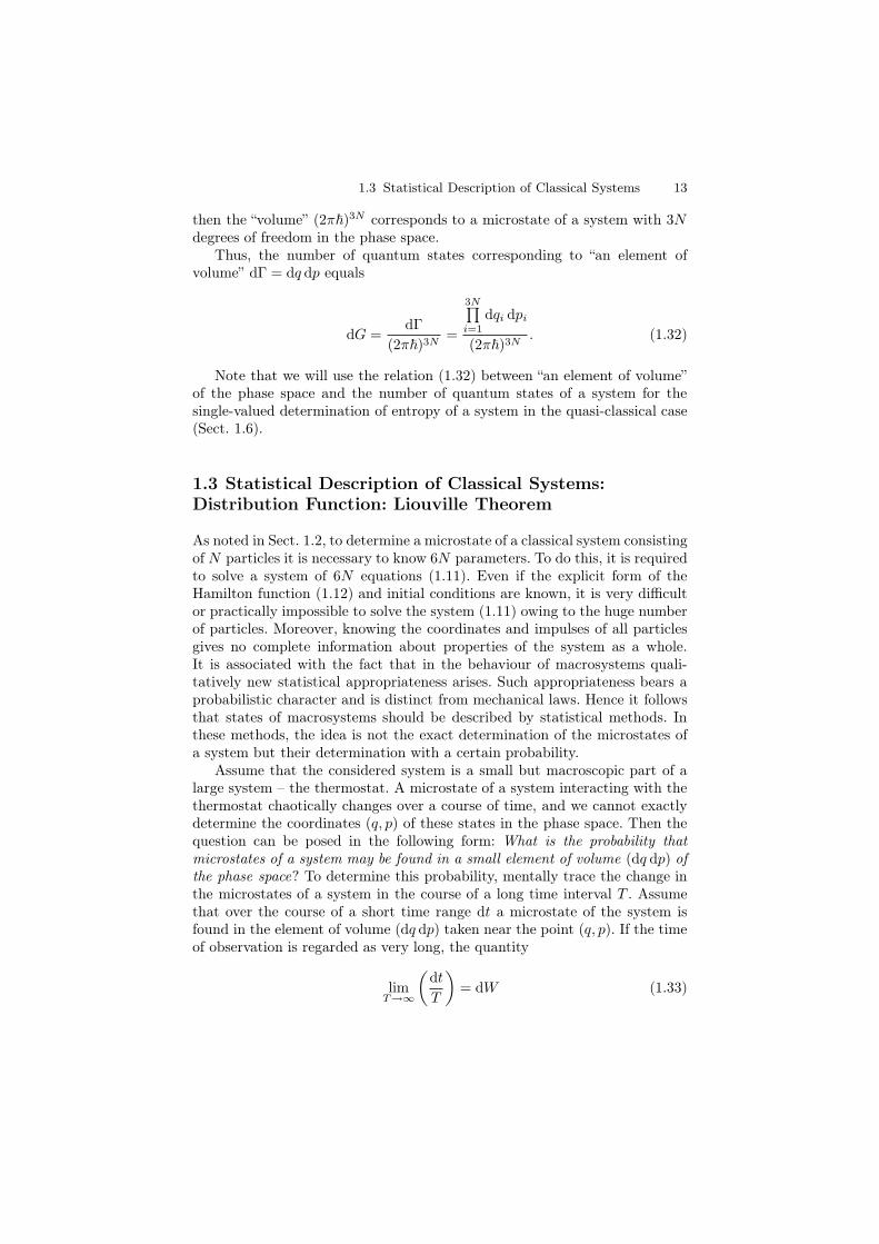
For classical systems, one phase point corresponds to each microstate andtherefore, formally, the “infinite” number of microstates corresponds to anyelement of the phase space. If, from the point of view of quantum mechanics,it is taken into account that the least “volume” of the phase space h = 2π�

(Fig. 1.4) corresponds to one state of a particle with one degree of freedom,

dqq

p

dp

h = 2πh

Fig. 1.4. The “volume” of the quantum state of a particle with one degree of freedom

1.3 Statistical Description of Classical Systems 13

then the “volume” (2π�)3N corresponds to a microstate of a system with 3Ndegrees of freedom in the phase space.

Thus, the number of quantum states corresponding to “an element ofvolume” dΓ = dq dp equals

dG =dΓ

(2π�)3N=

3N∏i=1

dqi dpi

(2π�)3N. (1.32)

Note that we will use the relation (1.32) between “an element of volume”of the phase space and the number of quantum states of a system for thesingle-valued determination of entropy of a system in the quasi-classical case(Sect. 1.6).

1.3 Statistical Description of Classical Systems:Distribution Function: Liouville Theorem

As noted in Sect. 1.2, to determine a microstate of a classical system consistingof N particles it is necessary to know 6N parameters. To do this, it is requiredto solve a system of 6N equations (1.11). Even if the explicit form of theHamilton function (1.12) and initial conditions are known, it is very difficultor practically impossible to solve the system (1.11) owing to the huge numberof particles. Moreover, knowing the coordinates and impulses of all particlesgives no complete information about properties of the system as a whole.It is associated with the fact that in the behaviour of macrosystems quali-tatively new statistical appropriateness arises. Such appropriateness bears aprobabilistic character and is distinct from mechanical laws. Hence it followsthat states of macrosystems should be described by statistical methods. Inthese methods, the idea is not the exact determination of the microstates ofa system but their determination with a certain probability.

Assume that the considered system is a small but macroscopic part of alarge system – the thermostat. A microstate of a system interacting with thethermostat chaotically changes over a course of time, and we cannot exactlydetermine the coordinates (q, p) of these states in the phase space. Then thequestion can be posed in the following form: What is the probability thatmicrostates of a system may be found in a small element of volume (dq dp) ofthe phase space? To determine this probability, mentally trace the change inthe microstates of a system in the course of a long time interval T . Assumethat over the course of a short time range dt a microstate of the system isfound in the element of volume (dq dp) taken near the point (q, p). If the timeof observation is regarded as very long, the quantity

limT→∞

(dtT

)= dW (1.33)


can be taken as the probability of the microstate of the system being foundin the element of volume (dq dp).

It is evident that the probability dW depends on around which point(q, p) = (q1, q2, . . . , q3N ; p1, p2, . . . , p3N ) the element of volume (dq dp) =3N∏i=1

dqi dpi is taken, and, naturally, the quantity dW ought to be directly

proportional to this element of volume (dq dp):

dW = ρ(q, p)dq dp. (1.34)

The coefficient of proportionality ρ(q, p) is the probability of the microstatefound in the unit volume of the phase space taken near the point (q, p) andis called the distribution function. From the geometrical point of view, ρ(q, p)is the density of phase points corresponding to the microstate of the systemnear the point (q, p) of the phase space, i.e. it characterizes the distributionof microstates of the system in the phase state.

Knowing the distribution function, we can calculate the mean statisti-cal value of any quantity L(q, p), depending on coordinates and impulses ofparticles of the system:

Lρ =∫L(q, p)ρ(q, p)dq dp. (1.35)

Notice that in reality the state of a system is determined by macroscopicquantities measured experimentally. Knowing the internal structure of thesystem, the mean value of the measured quantities with respect to time canbe immediately calculated:

Lt = limT→∞

1T

T∫0

L(q(t), p(t))dt. (1.36)

To do this, besides the explicit form of the dependence of the quantity L on qand p, it is necessary to know the dependences of the coordinates and impulsesof a particle on time, i.e. functions q = q(t) and p = p(t). And this means asolution of system of equations (1.11). Inasmuch as this system is unsolvable,the immediate calculation of Lt by (1.36) is not possible. In order to overcomethis difficulty, we assume that the mean value with respect to time (1.36) canbe replaced with the statistical mean (1.35):

Lt ⇒ Lρ. (1.37)

This supposition is called the ergodic hypothesis, and systems satisfying con-dition (1.37) are called ergodic systems. Henceforth, we will consider onlyergodic systems and omit the statistical index ρ, i.e. Lρ = L.

An advantage of calculation of the statistical mean value (1.35) lies in thefact that in this case it is sufficient to know dependences of the quantity L


on q and p, i.e. it is not necessary to know the time dependences of q and p.The explicit form of the function L(q, p) for different systems can be foundin classical mechanics. In the particular case, L can be the Hamilton functionH = E(q, p). However, as seen from (1.35), in order to find L, besides L(q, p)it is necessary to know the distribution function ρ(q, p). Finding the explicitform of this function is the basic task of statistical physics. It is necessaryto find such a distribution function in order that the mean statistical value,calculated with its aid, would coincide with the mean value with respect totime, i.e. condition (1.37) would be satisfied.

Properties of the distribution function. In order to find the explicit formof the distribution function, note its following properties.

1. The distribution function ought to satisfy the normalization condition. Itis evident that if we integrate the expression (1.34) over all the phasespace, we get the normalization condition∫

ρ(q, p)dq dp = 1, (1.38)

which means that the event of a microstate of a system being found atsome point or other of the phase space is real.

2. To define the second property of the distribution function, we introducethe concept of a statistically independent subsystem. Assume that the con-sidered system consists of two macroscopic subsystems. It is evident that inthe process of interaction of these subsystems, basically particles that arefound on the boundary, the number of which is much smaller than the totalnumber of particles in the subsystems, participate. Therefore, in a timerange which is less than the relaxation time, these subsystems can be con-sidered as self-dependent, i.e. the change in the state of one subsystem inthe given time interval does not influence the state of the other subsystem.Subsystems satisfying this condition are statistically independent.

Elements of volume of the phase space of the considered subsystems aredenoted by dq(1)dp(1) and dq(2)dp(2), respectively. Then probabilities ofmicrostates of the subsystems being found in these elements of volume havethe form

dW (1) = ρ1 dq(1)dp(1); dW (2) = ρ2 dq(2)dp(2). (1.39)

It is evident that the distribution function ρ1 depends on coordinates andimpulses of particles of the first subsystem, and ρ2 depends on coordinatesand impulses of particles of the second subsystem.

Mathematically, the statistical independence means that the probabilitydW = ρ dq dp of the microstate of the system consisting of two subsystemsfound in the element of volume dq dp = dq(1)dp(1)dq(2)dp(2) ought to equalthe product of the probability of the microstate of the first subsystem foundin the element of volume dq(1)dp(1) and the probability of the microstate ofthe second subsystem found in the element of volume dq(2)dp(2), i.e. dW =dW (1) · dW (2). In the explicit form


ρ dq dp = ρ1dq(1)dp(1) · ρ2dq(2)dp(2), (1.40)

orρ = ρ1 · ρ2. (1.41)

In the general case of a large system consisting of n0 number of subsystems,equality (1.41) takes the form

ρ = ρ1 · ρ2 · . . . · ρn0 =n0∏

α=1

ρα. (1.42)

Thus, the distribution function of a large system is the product of the dis-tribution functions of the statistically independent subsystems forming thelarge system. The converse is also true: if the distribution function of thewhole system can be presented in the form of the product of the distribu-tion functions of individual subsystems, these subsystems are statisticallyindependent.

If we take the logarithm of the equality (1.42), we can obtain the secondimportant property of the distribution function:

ln ρ =n0∑

α=1

ln ρα. (1.43)

This means that the logarithm of the distribution function of a large systemequals the sum of the logarithms of the distribution functions of the individualsubsystems; in other words, the logarithm of the distribution function of thesystem is an additive quantity.

3. Liouville theorem. The third property of the distribution function stemsfrom this theorem, according to which the distribution function is con-stant along the phase trajectory, i.e. ρ(q, p) = const. This is one of thedefinitions of the Liouville theorem. To prove this theorem, mentally keepa watch over microstates of the given subsystem for an extended time andsubdivide the time of observation into very small identical ranges. Imag-ine that phase points A1, A2, A3, . . . , An correspond to microstates of thesubsystem at instants of time t1, t2, t3, . . . , tn in the phase space.

Now assume that each phase point A1, A2, A3, . . . , An corresponds to amicrostate of one of the subsystems at the instant of time t. It is evidentthat the multitude of subsystems mentally formed in this way is a multitudeof states of identical subsystems (with identical Hamilton function) and iscalled the Gibbs statistical ensemble. The number of subsystems n enteringinto this ensemble ought to be very large.

A microstate of the statistical ensemble, i.e. positions of phase pointsA1, A2, . . . , An in the course of time changes and at the instant of time t′,is described by the multitude of the phase points A′1, A′2, . . . , A′n:

(A1, A2, . . . , An)t ⇒ (A′1, A′2, . . . , A

′n)t′ . (1.44)


If Δn phase points occupy an element of the phase volume ΔΓ, by definitionof the distribution function it can be written as

Δn = ρ(q, p, t)ΔΓ. (1.45)

For the pre-assigned ensemble, phase points do not disappear or arise. There-fore, the distribution function ρ(q, p, t) in the phase space ought to satisfythe continuity equation. In order to write the continuity equation in the6N -dimensional phase space, first remember its form in the usual three-dimensional space:

∂ρ

∂t+ div(ρυ) = 0. (1.46)

Here ρ(x, y, z, t) and υ(x, y, z, t) are the density and velocity of the flow ofpoints at the instant of time t, respectively. Equation (1.46) actually is thelaw of conservation of substance and can be written down in the form

∂ρ

∂t+ υ gradρ+ ρ div υ = 0. (1.47)

If we take into account that the sum of the first two terms is a total derivativeof the function ρ with respect to time, (1.47) takes the form:

dρdt

+ ρ div υ = 0. (1.48)

Then, by analogy with (1.48), for the continuity equation in the 6N -dimensional phase space we have:

dρ(q, p, t)dt

+ ρDivV = 0, (1.49)

where V is the vector of “velocity” in the 6N -dimensional phase space withcomponents q1, q2, . . . , q3N ; p1, p2, . . . , p3N ; dρ/dt is the velocity of the changein the density of phase points around the point (q, p); and DivV is the symbolof divergence in the 6N -dimensional phase space:

Div V =3N∑i=1

(∂qi∂qi

+∂pi

∂pi

). (1.50)

Taking into account the Hamilton canonical (1.11), we get:

3N∑i=1

(∂qi∂qi

+∂pi

∂pi

)=

3N∑i=1

(∂2H

∂qi∂pi− ∂2H

∂pi∂qi

)= 0. (1.51)

Thus, for the 6N -dimensional phase space

DivV = 0. (1.52)


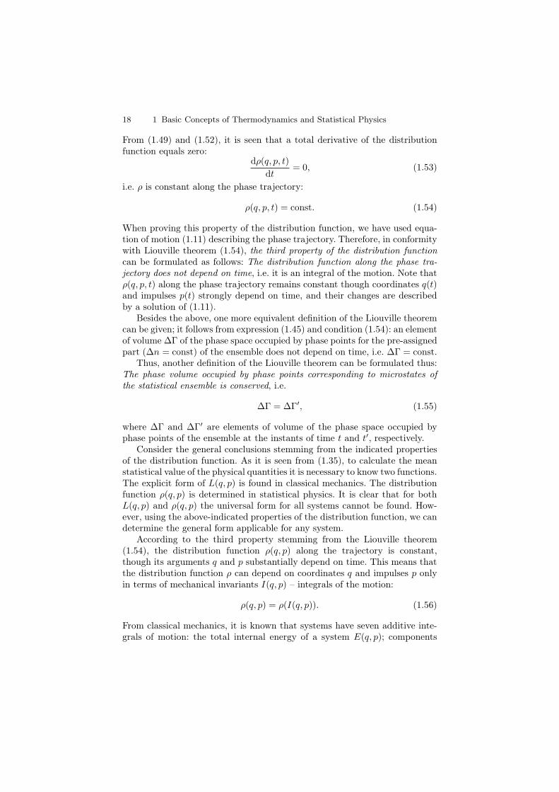
From (1.49) and (1.52), it is seen that a total derivative of the distributionfunction equals zero:

dρ(q, p, t)dt

= 0, (1.53)

i.e. ρ is constant along the phase trajectory:

ρ(q, p, t) = const. (1.54)

When proving this property of the distribution function, we have used equa-tion of motion (1.11) describing the phase trajectory. Therefore, in conformitywith Liouville theorem (1.54), the third property of the distribution functioncan be formulated as follows: The distribution function along the phase tra-jectory does not depend on time, i.e. it is an integral of the motion. Note thatρ(q, p, t) along the phase trajectory remains constant though coordinates q(t)and impulses p(t) strongly depend on time, and their changes are describedby a solution of (1.11).

Besides the above, one more equivalent definition of the Liouville theoremcan be given; it follows from expression (1.45) and condition (1.54): an elementof volume ΔΓ of the phase space occupied by phase points for the pre-assignedpart (Δn = const) of the ensemble does not depend on time, i.e. ΔΓ = const.

Thus, another definition of the Liouville theorem can be formulated thus:The phase volume occupied by phase points corresponding to microstates ofthe statistical ensemble is conserved, i.e.

ΔΓ = ΔΓ′, (1.55)

where ΔΓ and ΔΓ′ are elements of volume of the phase space occupied byphase points of the ensemble at the instants of time t and t′, respectively.

Consider the general conclusions stemming from the indicated propertiesof the distribution function. As it is seen from (1.35), to calculate the meanstatistical value of the physical quantities it is necessary to know two functions.The explicit form of L(q, p) is found in classical mechanics. The distributionfunction ρ(q, p) is determined in statistical physics. It is clear that for bothL(q, p) and ρ(q, p) the universal form for all systems cannot be found. How-ever, using the above-indicated properties of the distribution function, we candetermine the general form applicable for any system.

According to the third property stemming from the Liouville theorem(1.54), the distribution function ρ(q, p) along the trajectory is constant,though its arguments q and p substantially depend on time. This means thatthe distribution function ρ can depend on coordinates q and impulses p onlyin terms of mechanical invariants I(q, p) – integrals of the motion:

ρ(q, p) = ρ(I(q, p)). (1.56)

From classical mechanics, it is known that systems have seven additive inte-grals of motion: the total internal energy of a system E(q, p); components

1.4 Microcanonical Distribution: Basic Postulate of Statistical Physics 19

of the impulse Px, Py, Pz; and components of the moment of the impulseMx,My,Mz of the system as a whole. Note that the frame of reference can beso connected with the body (the system) that in the given frame of referenceP and M would be equal to zero. Then, in this frame of reference the onlymechanical invariant – the total internal energy E(q, p) – remains, and as aresult dependence (1.56) can be written down in the form

ρ(q, p) = ρ(E(q, p)). (1.57)

Such a dependence of the distribution function ρ(q, p) indicates the exclusivelyimportant role of the internal energy E(q, p) in statistical physics.

Thus, we get the most general and fundamental property of the distri-bution function: The distribution function ρ(q, p) depends only on the totalinternal energy of a system E(q, p).

And what is the explicit form of this dependence? To this question, auniversal answer for any system does not exist. We consider a concrete system.

Assume that the considered system consists of several subsystems. Then,taking into account the condition of additivity of energy (1.2) and ln ρ (1.43),we see that the logarithm of the distribution function of any α-subsystem candepend on its energy Eα as follows:

ln ρα = Aα + βEα(q, p). (1.58)

The constants Aα and β here are found from some specified conditions. It isevident that the coefficient β ought not to depend on the number of the sub-system and is identical for all subsystems. Only in this case, for all the systemln ρ(q, p) and, consequently, the distribution function ρ(q, p) itself satisfies thecondition (1.57): i.e. ρ(q, p) depends only on the total internal energy of thesystem: E =

∑αEα.

It should be noted that just the distribution function of a system found inthe thermostat, i.e. the Gibbs canonical distribution (see Chap. 4), has sucha general appearance (1.58): or

ρα = exp(Aα + βEα(q, p)). (1.59)

1.4 Microcanonical Distribution:Basic Postulate of Statistical Physics

The microcanonical distribution is concerned with completely isolated sys-tems. Owing to the absence of any interaction with the surrounding medium(ΔA = 0, ΔΘ = 0, ΔN = 0), its energy remains fixed as E0 = const, i.e. inwhatever microstate the system is found, its total internal energy is

E(q, p) = E0. (1.60)


Microstates satisfying this condition are called possible states. In the abstractphase space, (1.60) is an equation of a specified “hypersurface”. Energy of allmicrostates corresponding to phase points on this surface is identical, andE0 = const. Therefore this hypersurface is called the isoenergetic surface. Itis evident that the system cannot be found in microstates to which phasepoints outside this surface E(q, p) �= E0 correspond. These states are calledimpossible states.

The explicit form of the distribution function for completely isolated clas-sical systems that are found in the thermodynamic equilibrium is determinedon the basis of the postulate of statistical physics.

The basic postulate of statistical physics is as follows: If a completely iso-lated system is found in the thermodynamic equilibrium state, the probabilityof it being found in any possible microstate is identical, i.e. preference can begiven to none of the possible states.

Mathematically, this postulate can be expressed in the form

ρ(q, p) =

{C = const, at E(q, p) = E0,

0, at E(q, p) �= E0.(1.61)

For the distribution function, expression (1.61) has the appearance

ρ(q, p) = Cδ(E(q, p) − E0). (1.62)

This distribution function is called the microcanonical distribution. The con-stant C is determined from the normalization condition of the distributionfunction (1.38):

∫ρ(q, p)dq dp = C

∫δ(E(q, p) − E0)dq dp = 1. (1.63)

Recall that the δ-function entering into expression (1.62) has the followingproperties:

1.∫δ(x− a)dx = 1,

2.∫f(x)δ(x − a)dx = f(a), (1.64)

3.∫f(x)δ[φ(x)]dx =

∑s

f(xs)|φ′(xs)| ,

where xs are roots of the equation φ(xs) = 0, and a is an arbitrary constant.In order to use the second property of the δ-function (1.64), in (1.63) passfrom the integral over dq dp ≡ dΓ to the integral over dE. Then we get

C

∫δ(E(q, p) − E0)dq dp = C

∫δ(E(q, p) − E0)

dΓdE

dE = 1.

1.4 Microcanonical Distribution: Basic Postulate of Statistical Physics 21

0 E0

ρ(q, p)

E(q, p)

Fig. 1.5. The microcanonical distribution for isolated classical systems

HereC =

1(dΓ/dE)E=E0

=1

Ω(E0)(1.65)

is the normalizing constant.Hence, it is seen that the quantity Ω(E0) = (dΓ/dE )E=E0 represents

the “volume” of the phase space found between two hypersurfaces, differingfrom one another by one energetic unit and taken around the isoenergetichypersurface E(q, p) = E0.

As a result, the distribution function for isolated classical systems – themicrocanonical distribution – takes the form

ρ(q, p) =1

Ω(E0)δ(E(q, p) − E0). (1.66)

The microcanonical distribution is schematically depicted in Fig. 1.5.Note that (1.66) is a mathematical expression of the basic postulate of

statistical physics. The justification of this postulate is corroborated by thecoincidence of the results obtained by use of (1.66) with the experimentalresults.

For isolated systems, with the aid of the microcanonical distribution themean value of any physical quantity depending on energy L(q, p) = L(E(q, p))can be computed:

L =∫L(E(q, p))

1Ω(E0)

δ(E(q, p) − E0)dq dp. (1.67)

If with the aid of the replacement

dq dp = dΓ =dΓdE

dE (1.68)

we pass from the integral over dΓ to the integral over dE and take into account(1.65), for the mean value we get

L = L(E0). (1.69)

In the particular case when L(E(q, p)) = E(q, p), for the mean value of energyof the system we have

E(q, p) = E0. (1.70)


1.5 Statistical Description of Quantum Systems:Statistical Matrix: Liouville Equation

Imagine that the motion of particles of the considered macroscopic systembears quantum character. Inasmuch as the number of particles in the systemis very large, the purely quantum mechanical description of the system aswell as for classical systems is practically impossible. In fact, for the quantummechanical description of a system it is necessary to solve (1.16) and findthe wave function Ψn, depending on 3N number of variables – coordinatesof all particles. Furthermore, the wave function Ψn can be used to find thequantum mechanical mean value L of the physical quantity L. The practicalimpossibility of working with this problem is evident.

Another principal difficulty is associated with the fact that a system cannotbe found in the purely stationary quantum state, inasmuch as its energy spec-trum is continuous. In nature, a completely isolated system does not exist.Each system to some extent interacts with the surrounding medium andthe energy of this interaction is more of the difference between energy lev-els. Therefore, the macroscopic system being found in the stationary state isimpossible. For this reason, the macroscopic system is found not in the purelyquantum state but in “the mixed” state. According to quantum mechanics,in “a mixed” state the system is described not by the stationary wave func-tion, but by the density matrix. In statistical physics, it is called the statisticalmatrix.

Impossibility of the stationary state of a macroscopic system also followsfrom the uncertainty principle for energy. Indeed, the difference of energiesof two adjacent levels ΔE = (En+1 − En) ought to be much more than theuncertainty of energy:

δE ∼ �

Δt. (1.71)

To fulfill this condition, the time of measurement Δt ought to be infinitelylarge. In reality, however, Δt is finite. Therefore, in the range of the uncertaintyof energy δE, several energy levels can be found and, consequently, it cannotbe asserted that the system is found in some specified stationary state.

Thus, inasmuch as the quantum mechanical description of the system isimpossible, the problem needs to be solved by statistical methods. To do this,we proceed as follows. Separate one subsystem, which is a small part of a largesystem. Suppose that the subsystem does not interact with the surroundings.Then, we can speak about “the stationary state” of the subsystem. The wavefunction of the subsystem in these stationary states is denoted by ψn(q).Here, q are coordinates of all particles of the system, and n is the totalityof quantum numbers determining its stationary state. Let the energy of thisstationary state be En.

Assume that at a certain instant of time the state of the subsystem isdescribed by the wave function Ψ(t), which can be expanded into a series

1.5 Statistical Description of Quantum Systems 23

with respect to orthonormalized wave functions ψn(q):

Ψ(t) =∑

n

Cnψn(q), (1.72)

where the coefficient Cn depends on time

Cn ∼ exp(− iEnt

�

), (1.73)

and satisfies the normalization condition∑n

|Cn|2 = 1. (1.74)

The mean value of a physical quantity L corresponding to the operator L isdefined as follows:

L =∫

Ψ∗LΨ dq. (1.75)

If we use the expansion (1.72), for L we get

L =∑nm

C∗nCmLnm, (1.76)

whereLnm =

∫ψ∗n(q)Lψm(q)dq (1.77)

is the matrix element of the physical quantity L corresponding to theoperator L.

If we introduce the notation

C∗nCm ⇒Wmn, (1.78)

we get the formula to calculate the mean value:

L =∑mn

WmnLnm. (1.79)

The totality of quantities Wmn is called the statistical matrix. If we denotethe statistical operator corresponding to this matrix by W , expression (1.79)takes the form

L =∑

n

(W L)nn. (1.80)

Diagonal elements of the statistical matrix Wnn ≡Wn show the probability ofthe system being found in the stationary state n. Therefore Wn in the quan-tum statistics corresponds to the distribution function ρ(q, p) in the classicalstatistics:

ρ(q, p) ⇒Wn, (1.81)


and the normalization condition (1.38) has the appearance∑

n

Wn = 1. (1.82)

Recall that for a classical system the distribution function ρ(q, p) determinesthe probability of the system that is found in a microstate corresponding to thephase point (q; p). And in quantum systems, Wn means the probability of thesystem that is found in a microstate with energy En, which is determined bythe totality of quantum numbers n.

For classical systems, the distribution function ρ(q, p) possesses the prop-erty stemming from the Liouville theorem: the distribution function is anintegral of the motion and therefore depends only on mechanical invariants(1.56). In quantum systems, for the statistical matrix Wnm a theorem anal-ogous to the Liouville theorem can be proved. To do this, using (1.73) writedown the derivative of the statistical matrix with respect to time. Then we get

∂

∂t(C∗nCm) =

i

�(En − Em)C∗nCm, (1.83)

or, if we use notations (1.78),

∂

∂tWmn =

i

�(En − Em)Wmn. (1.84)

The right-hand side of this equation can be presented in the form

(En − Em)Wnm =∑

k

(WmkHkn − HmkWkn). (1.85)

Here Hmn is the matrix element of the Hamilton operator H . In the energeticrepresentation, Hmn is a diagonal matrix:

Hmn = Enδmn. (1.86)

If we take this into account, the entry of (1.85) becomes clear.As a result, (1.84) takes the form

∂

∂tWmn =

i

�

∑k

(WmkHkn − HmkWkn). (1.87)

Equation (1.87) can be also written down in the matrix form, i.e. for theoperator of the density matrix W ,

∂

∂tW =

i

�(WH − H W ). (1.88)

This equation, as well as (1.87), is called the Liouville equation.

1.5 Statistical Description of Quantum Systems 25

As seen from the Liouville equation, to fulfill the stationary condition∂W/∂t = 0, the operator W ought to commutate with the Hamilton operatorH of the system:

WH − H W = 0. (1.89)

Physical quantities corresponding to the operator that commutates with theHamilton operator are conservation quantities. Therefore, according to (1.89),it can be asserted that the statistical matrix is an integral of the motion.

In quantum statistics, this conclusion is an analogue of the Liouvilletheorem (1.54) in classical statistics.

From the energetic presentation of the statistical matrix, one more of itsproperty follows. Indeed, as seen from the Liouville equation (1.84), to fulfillthe stationary condition (∂Wmn/∂t = 0) the following ought to take place:

(En − Em)Wmn = 0. (1.90)

And to fulfill this condition, the matrix element Wmn ought to be diagonal:

Wmn = Wnδmn. (1.91)

With regard to (1.91), the formula for the mean value (1.79) takes the form

L =∑

n

WnLnn. (1.92)

As can be seen, to calculate the mean value of any physical quantity L it is suf-ficient to know the distribution function Wn and only the diagonal elementsof the matrix Lnn . For the considered system, Lnn is found from quantummechanics. And the finding of the explicit form of the distribution functionWn is the task of statistical physics. Naturally, a universal expression for Wn

applicable to any system does not exist. However, as is known, in quantumstatistics the Liouville theorem is fulfilled, too, i.e. Wn is a conservation quan-tity. And this means that the dependence Wn on the totality of the quantumnumbers n is expressed by conservation quantities, namely, by En:

Wn = W (En). (1.93)

This property is an analogue of the property of the distribution function (1.61)in classical statistics.

The explicit form of the function W (En) is different for different physi-cal systems. Assume that the considered system with energy E = En consistsof statistically independent subsystems. If we denote the energy of theα-subsystem by Enα , the energy of the complete system is

En =∑α

Enα , (1.94)

where nα is the totality of quantum numbers determining the state of theα-subsystem, and n is the totality of quantum numbers determining the stateof the whole system, i.e. n⇒ n1, n2, . . . nα.


Inasmuch as the subsystems are statistically independent, the distributionfunction Wn ought to possess the property analogous to the property of ρ(q, p)in classical statistics (1.43):

ln Wn =∑α

ln Wnα , (1.95)

i.e. in the quantum case the logarithm of the distribution function is an addi-tive quantity, too. Then, the logarithm of the distribution function can bepresented in the form

ln W (Enα) = Aα + βEnα , (1.96)

where Enα is energy of the α-subsystem; Aα is a constant, which is found fromthe normalization condition and depends on the number of the subsystem; andthe coefficient β ought not to depend on the number of the subsystem, sinceonly in this case conditions (1.95) and (1.94) are fulfilled at the same time.

Notice that the canonical distribution for systems in the thermostat hasthe same appearance as (1.96).

Consider the microcanonical distribution for isolated quantum systemswith the pre-assigned energy E = E0 = const. As noted above, the energyspectrum of macroscopic systems is continuous. Denote by dG the number ofquantum states in an infinitely small range of energy dE taken around thegiven value of energy E.

If it is supposed that the system consists of several subsystems, then

dG =∏α

dGα, (1.97)

where dGα is the number of quantum states in an infinitely small range ofenergy dE, taken close to the given value of energy Eα of the subsystem withnumber α.

Notice that (1.97) corresponds to the relationship

dΓ =∏α

dΓα (1.98)

for the classical case, which means that an element of volume of the phasespace of the whole system equals the product of elements of volumes of thephase space of individual subsystems.

For an isolated system, quantum states dG falling in the range of energydE can be considered as possible states. According to the basic postulate ofstatistical physics, the probability of the system found in any microstate isidentical, i.e. preference can be given to none of them. On the other hand,the probability dW of the system found in any of the states dG ought to beproportional to the number dG. Then it can be written as

dW = const δ(E − E0)∏α

dGα. (1.99)

1.6 Entropy and Statistical Weight 27

Equation (1.99) is called the microcanonical distribution for quantum systems.Here the δ(E − E0) function shows the isolatedness of the system, and

E =∑α

Eα (1.100)

is the total energy of the system.

1.6 Entropy and Statistical Weight

We introduce one of the basic concepts of thermodynamics and statisticalphysics – entropy of a system. Entropy, as well as energy, is a function ofstate, i.e. it determines the microscopic state of a system.

At first, consider the concept of the statistical weight of a system, whichis closely associated with entropy. To do this, suppose that the consideredquantum system is found in the thermodynamic equilibrium state. Subdividethis system into a multitude of subsystems. Let n be the totality of quantumnumbers determining a microstate of any subsystem with energy En, andWn = W (En) be the probability of the system found in the given microstate.Pass from the distribution over microstates W (En) to the distribution overenergy w(E). It is known that the energy spectrum of a macroscopic systemis almost continuous, and therefore a multitude of energy levels correspondingto the quantum states accounts for a sufficiently small range of energies. Inorder to find the probability w(E)dE of the system found in the state withenergy in the range of E and E + dE taken close to E, it is necessary tomultiply the function W (E) by the number of quantum states (microstates)accounting for the range of energy dE.

If we take into account that the number of these microstates is

dG(E) =dG(E)

dEdE = g(E)dE, (1.101)

the distribution function over energies takes the form

w(E) = g(E)W (E). (1.102)

Hereg(E) =

dG(E)dE

(1.103)

is the function of the density of quantum states, i.e. the number of quantumstates accounting for a unit range of energy taken close to E, and G(E) is thetotal number of all the quantum states with energy less than E.

Even without knowing the explicit form of the distribution function w(E),it can be asserted that a subsystem in thermodynamic equilibrium ought tobe found most of the time in states close to the mean value of energy E.


E

E0

w(E)

w(E)

ΔE

Fig. 1.6. The distribution function over energy

Therefore, the distribution function w(E) over energy ought to have a sharpmaximum at E = E (Fig. 1.6).

According to the normalization condition∫w(E)dE = 1. (1.104)

This geometrically means that the area under the curve w(E) ought to beequal unity.

If the curve depicted in Fig. 1.6 is approximately replaced by a rectanglewith the height w(E) and width ΔE, condition (1.104) can be presented inthe form

w(E)ΔE = 1, (1.105)

where ΔE is called the width of the distribution curve over energy.Taking into account the distribution function (1.102) in (1.105), we get

W (E)ΔG = 1. (1.106)

Here,ΔG = g(E)ΔE (1.107)

is the number of microstates accounting for the range of energies ΔE of thesubsystem and is called the statistical weight of a macrostate of the systemwith energy E = E.

The statistical weight ΔG shows the number of microstates correspondingto one pre-assigned macrostate of the system. Therefore, ΔG characterizesthe degree of the internal chaoticity of the system.

The statistical weight of a closed system, in conformity with (1.97), can bepresented as the product of statistical weights of the individual subsystems:

ΔG =∏α

ΔGα, (1.108)

where ΔGα = ΔG(Eα) is the statistical weight of the α-subsystem.In statistical physics, apart from the statistical weight, a more convenient

function, also characterizing the degree of chaoticity of a system, is accepted.This function is defined as a logarithm of the statistical weight:

1.6 Entropy and Statistical Weight 29

S = k0 ln ΔG (1.109)

and is called the entropy of a system. Here k0 is the Boltzmann constant. Asis seen, entropy cannot be negative, i.e. S ≥ 0, since the statistical weightΔG ≥ 1. Note that entropy of a system, as also the energy, in conformitywith (1.108) and (1.109), possesses the property of additivity, i.e.

S =∑

α

Sα. (1.110)

Here, Sα = k0 ln ΔGα is entropy of the α-subsystem.Thus, it can be asserted that entropy is a function of the state of a macro-

scopic system and characterizes the degree of its internal chaoticity; entropyhas only a statistical sense; entropy cannot be spoken of separately for a givenparticle.

If we take into account (1.106) in (1.109), entropy can be expressed by thedistribution function

S = −k0 ln W (E). (1.111)

Inasmuch as, according to (1.96), the logarithm of the distribution func-tion is a linear function of energy, lnW (E) can be replaced with the meanlnW (E), i.e.

ln W (E) = ln W (E). (1.112)

Then, the expression of entropy (1.111) takes the form

S = −k0

∑n

Wn ln Wn. (1.113)

We now consider classical systems in the quasi-classical approximation. In thiscase, using the normalization condition for classical systems consisting of Nparticles, ∫

ρ(q, p)dΓ = 1, (1.114)

where dΓ = dq dp =3N∏i

dqi dpi is an element of volume of the phase space,

and therefore we can pass from the distribution over microstates ρ(q, p) to thedistribution over energies ρ(E). To do this, rewrite the condition (1.114) inthe form ∫

ρ(E(q, p))dΓdE

dE = 1, (1.115)

or ∫ρ(E(q, p))(2π�)3Ng0(E)dE = 1. (1.116)

Here,

g0(E) = (2π�)−3N dΓdE

(1.117)


is the function of the density of states of quasi-classical systems.As is seen from (1.116),

ρ(E) = (2π�)3Nρ(E(q, p))g0(E) (1.118)

is the distribution function over energy. Then condition (1.116) takes the form∫ρ(E)dE = 1. (1.119)

Taking into account that ρ(E) takes on a maximum value at E = E, (1.119)can be roughly presented as

ρ(E)ΔE = 1. (1.120)

Here ΔE is the width of the distribution curve (Fig. 1.6). If substitute (1.118)into (1.120), we get

(2π�)3Nρ(E(q, p))ΔG = 1, (1.121)

whereΔG = g0(E)ΔE (1.122)

is the number of microstates accounting for the range of energy ΔE takenclose to energy E = E in the quasi-classical case, i.e. the statistical weightof the macrostate with energy E = E. Then entropy can be presented inthe form

S = k0 ln ΔG = k0 ln g0(E)ΔE. (1.123)

If the value of g0(E) from (1.117) is taken into account, for the quasi-classicalcase entropy can be presented as

S = k0 lnΔqΔp

(2π�)3N. (1.124)

In the quasi-classical case, entropy can be also expressed by the distributionfunction over microstates. To do this, take into account (1.121) and (1.123).Then we get

S = −k0 ln[(2π�)3Nρ(E(q, p))]. (1.125)

On the basis of property (1.58) of the distribution function, we can replace

ln ρ(E(q, p)) = ln ρ(E(q, p)). (1.126)

As a result, for entropy we get

S = −k0

∫ρ(q, p) ln

[(2π�)3Nρ(q, p)

]dq dp. (1.127)

From additivity of entropy (1.110), one more its property stems. If we dividethe width of the distribution function ΔE (Fig. 1.6) by the number of

1.7 Law of Increasing Entropy: Reversible and Irreversible Processes 31

energy levels ΔG in this range, we get the distance between adjacent energylevels:

D(E) =ΔEΔG

= ΔE e−S(E)/k0 . (1.128)

From the property of additivity, it follows that the more the amount of sub-stance (the number of particles N) in a system, the more is the entropyof the system S(E) and the denser the energy levels. Thus, with increasingamount of substance in a system, the distance between adjacent energy levelsexponentially decreases.

In conclusion, once more recall the basic properties of entropy:

1. Entropy is a function of state and characterizes the degree of its internalchaoticity. The more the entropy, the more is the chaoticity, and vice versa;the less the entropy, the more is the ordering of the system.

2. Entropy has only a statistical sense; it cannot be spoken of for a separateparticle.

3. Entropy cannot be negative, i.e. S ≥ 0.4. Entropy is an additive quantity, i.e. S =

∑αSα.

5. Entropy characterizes the density of levels in the energy spectrum of asystem. The more the entropy, the denser are the energy levels.

6. Entropy of a system in the thermodynamic equilibrium state takes on amaximum value. This property follows from the law of increasing entropy,which is further discussed in Sect. 1.7 below.

1.7 Law of Increasing Entropy:Reversible and Irreversible Processes

In Sect. 1.6, we introduced the concept of entropy of an isolated system foundin thermodynamic equilibrium. The question arises whether entropy can bespoken of for a system that is not in thermodynamic equilibrium. A positiveanswer to this question can be given, i.e. the concept of entropy for thermody-namic non-equilibrium systems can also be introduced. To substantiate this,imagine that the considered closed system is not found in the thermodynamicequilibrium state, and its relaxation time is τ . If we study the system in thetime range Δt < τ , it is evident that the system is in the non-equilibrium state(Fig. 1.7a) and, naturally, we cannot speak of a specified value of entropy ofthe system. However, if we subdivide the considered system into small sub-systems, the relaxation time τα7 of each of them (assume with number α) willbe less than the time of observation Δt, i.e. τα < Δt (Fig. 1.7b). As can beseen from the figure, for a very small time τα the subsystem passes onto itslocal equilibrium state (the quantity Lα tends to its local equilibrium valueL0α). And it can be said that for all the time of observation Δt, the subsystem

7 With a decrease in dimensions of the subsystem its relaxation time decreases.


L0 L0α

τ0

(a) (b)t τα

0 tDt

L(t) Lα (t)

Dt

Fig. 1.7. The relaxation of the thermodynamical parameter: (a) - for system; (b) -for subsystem

is found in this local equilibrium state. Consequently, the concept of entropySα = S(Eα) can be introduced for each subsystem found in the local equi-librium state. Inasmuch as entropy is an additive quantity, we can speak ofthe instantaneous value of entropy of a large non-equilibrium system, havingdefined it as S(t) =

∑αSα(Eα).

According to the first postulate of thermodynamics, in the course of timean isolated non-equilibrium system ought to pass into the equilibrium state.The question arises as to how entropy of the system S(t) changes as a resultof this process.

In order to answer this question, use the microcanonical distribution func-tion (1.99) for isolated systems with energy E0 and pass from the distributionover microstates to the distribution over energy. Then, (1.99) takes the form

dW = const δ(E − E0)∏α

dGα

dEαdEα. (1.129)

If we replace the derivative dGα/dEα in this distribution by the ratioΔGα/ΔEα and make use of the expression of entropy of the α-subsystem,stemming from definition (1.109)

ΔGα = exp(Sα(Eα)k0

), (1.130)

we get

dW = const δ(E − E0) eS/k0∏α

dEα

ΔEα, (1.131)

where S =∑αSα(Eα) is entropy of the isolated system. Inasmuch as the

range of energy ΔEα very weakly depends on energy compared with the factoreS/k0 , it can be regarded as constant and the distribution function over energy(1.131) takes the form

dW = const δ(E − E0)eS/k0∏α

dEα. (1.132)

1.7 Law of Increasing Entropy: Reversible and Irreversible Processes 33

The obtained distribution function (1.132) is the probability of the subsystemsfound in states with energies E1, E2, . . . , Eα, . . . in the ranges of energy E1 +dE1, E2 + dE2, . . . , Eα + dEα, . . ., respectively. Here the δ(E − E0) functionprovides the isolatedness of the system, i.e. E =

∑αEα = E0 = const.

As seen from (1.132), the distribution function over energies of an isolatedsystem having the above-indicated physical sense very strongly and expo-nentially depends on entropy of the system, i.e. S = S(E1, E2, . . . , Eα, . . .).Therefore, the greater the probability of the considered macrostate of the sys-tem, the higher is the entropy of this state. It is known that the probability ofan isolated system found in thermodynamic equilibrium state is maximum. Inthis state, energy of subsystems ought to be equal to its mean value, Eα = Eα.Thus, entropy of an isolated system in thermodynamic equilibrium state hasthe maximum value:

S(E1, E2, . . . , Eα, . . .) = Smax. (1.133)

Conclusion: If an isolated system at a certain instant of time is not foundin thermodynamic equilibrium state, in the course of time internal processesproceed in such a direction, as a result of which the system comes to its equilib-rium state and at that entropy of the system increases, reaching its maximumvalue. This assertion is called the Law of Increasing Entropy or the SecondLaw of Thermodynamics. The law in such a form was formulated by Clausiusin 1865, and statistically substantiated by Boltzmann in 1870.

Note that on a system such a process can be performed at which eachmacroscopic state will be in thermodynamic equilibrium and entropy doesnot change. Taking into account this case also, the law of increasing entropyin the general form can be formulated as follows: Entropy of an isolated systemnever decreases; it either increases or, in the particular case, remains constant.

In conformity with this, processes proceeding in all macroscopic systemscan be subdivided into two groups (Fig. 1.8):

dS/dt > 0 − irreversible processdS/dt = 0 − reversible process. (1.134)

Reversible process

0

Irreversible process

t

S = const

∂ S/∂ t>0S(t)

Smax

Fig. 1.8. The time dependence of entropy for irreversible and reversible processes


Irreversible processes cannot proceed in the reverse direction, inasmuch asin that case the entropy decreases, but this contradicts the law of increasingentropy. In nature, we frequently come across irreversible processes. Diffu-sion, thermal conductivity, expansion of a gas, etc. can serve as examples ofirreversible processes.

A reversible process can proceed in direct and reverse directions. In thiscase, a system passes through identical equilibrium macroscopic states, sincein this case entropy in both the directions does not change. In nature, it canbe said that reversible processes do not exist, and they can be created onlyapproximately by artificial methods. Compression or expansion of a gas foundunder a piston in a cylinder is one example of the simple adiabatic process.

An adiabatic process is a reversible process. Processes proceeding suffi-ciently slowly in adiabatically isolated (ΔQ = 0) systems are called adiabatic.We can show that in such processes entropy does not change: dS/dt = 0, i.e.the process is reversible. To do this, consider the simplest case: a gas under apiston in an adiabatically isolated cylinder (Fig. 1.9).

As the external parameter, take the volume of the gas under the piston,which for the given cylinder is determined by the height l. By changing thisheight, we can increase or decrease the volume of the gas. Inasmuch as thechange in entropy with time is related to the change in volume, we can write

dSdt

=dSdl

· dldt. (1.135)

Suppose that the piston moves sufficiently slowly; then the change in entropywith time can be expanded into a series in powers of l = dl/dt:

dSdt

= A0 +A1dldt

+A2

(dldt

)2

+ · · · (1.136)

The constants A0 and A1 in this series ought to be equal to zero. The constantA0 equals zero because at l = 0 the state of the system does not changeand entropy remains constant, i.e. dS/dt = 0; A1 equals zero because whenchanging the sign of l (the motion of the piston down and up), dS/dt changesits sign, which contradicts the law of increasing entropy (dS/dt ≥ 0). Thus,

l

l > 0.

l < 0.

Fig. 1.9. An adiabatic process

1.8 Absolute Temperature and Pressure: Basic Thermodynamic Relationship 35

dSdt

= A2

(dldt

)2

. (1.137)

If we take into account (1.135), we get

dSdl

= A2dldt. (1.138)

Hence it is seen that as the velocity of the piston tends to zero (l → 0),the change in entropy of the system with respect to the external parameter ltends to zero: dS/dl = 0, i.e. when the change in volume of the adiabaticallyisolated gas is slow, the processes of expansion or compression are adiabaticallyreversible.

Thus, we have seen that the processes of expansion or compression arereversible (dS/dl = 0) if the piston moves with a very small velocity. Thenthe following question arises: In reference to which velocity ought the velocityof the piston be small? In order to answer this question, take a look at theprocess of compression or expansion of the gas. If the piston moves down(l < 0), immediately under the piston the instantaneous density of the gasincreases. The velocity of motion of the piston ought to be such that at anyinstance of time, i.e. at any position of the piston, the density of the gaseverywhere would be identical, i.e. the gas would be found in thermodynamicequilibrium. An analogous situation arises also during the upward motionof the piston (l > 0): as the piston moves up, the gas ought to fill up thevacuum forming under the piston, in order that the density would be identicaleverywhere and equilibrium would be attained. It is apparent that during themotion of the piston the process of regaining uniform distribution of particlesof the gas occurs with the speed of sound. Therefore, in order that the processwould be adiabatic, the velocity of the motion of the piston ought to be lessthan the speed of propagation of sound υ0 in the gas:

∣∣∣∣dldt∣∣∣∣� υ0. (1.139)

If we take into account that the speed of sound in most gases is on the order of350 m/s, the piston can be moved with a sufficiently large velocity, satisfyingcondition (1.139), and the adiabaticity of the process is not violated.

1.8 Absolute Temperature and Pressure:Basic Thermodynamic Relationship

In Sect. 1.7 we became acquainted with three thermodynamic quantities: vol-ume V , internal energy E(q, p) and entropy S(E). Of these, volume is anexternal parameter, and energy and entropy are internal ones. Energy hasboth a mechanical and a statistical sense, and entropy has only a statistical


a b

E1

E2

S2

S1

V2

V1

Fig. 1.10. The thermal equilibrium of two subsystems

sense. The change in one of these quantities induces a change in the oth-ers. Derivatives of these quantities are also thermodynamic parameters: forinstance, absolute temperature and pressure. We consider them separately.

Absolute temperature. Assume that an isolated system with energy E0 =const in thermodynamic equilibrium consists of two subsystems with energy,entropy and volume E1, S1, V1 and E2, S2, V2, respectively (Fig. 1.10). As aconsequence of the additivity of energy and entropy, we have

E = E1 + E2, (1.140)

andS = S1(V1, E1) + S2(V2, E2). (1.141)

Assume that the boundary of division of the two subsystems ab (Fig. 1.10) isimmovable; therefore, volumes V1 and V2 do not change but energies of thesystems E1 and E2 and also entropies S1 and S2 can change.

Taking into account E2 = E−E1, notice that entropy of an isolated systemdepends only on one independent variable E1, i.e. S = S(E1). According tothe law of increasing entropy, in thermodynamic equilibrium entropy of anisolated system ought to be maximum. For this, it is necessary to fulfill thecondition

∂S

∂E1=(∂S1

∂E1

)V1

+(∂S2

∂E2

)V2

∂E2

∂E1= 0. (1.142)

Since ∂E2/∂E1 = −1, from (1.142) we get8

(∂S1

∂E1

)V1

=(∂S2

∂E2

)V2

. (1.143)

If an isolated system in thermodynamic equilibrium is subdivided into n arbi-trary subsystems, the condition of thermodynamic equilibrium (1.143) in thegeneral form can be presented as

8 Here and everywhere a quantity, indicated at the foot of the bracket when takingthe derivate, is regarded as constant.

1.8 Absolute Temperature and Pressure: Basic Thermodynamic Relationship 37(∂S1

∂E1

)V1

=(∂S2

∂E2

)V2

= · · · =(∂Sn

∂En

)Vn

. (1.144)

Hence it is seen that if an isolated system is found in thermodynamic equi-librium, there exists the quantity (∂S/∂E)V , which is identical in any part ofthe system. The reciprocal value of this quantity is denoted by T :(

∂E

∂S

)V

= T (1.145)

and is called the absolute temperature or, in brief, temperature. Then conditionof thermodynamic equilibrium or maximum entropy (1.144) takes the form

T1 = T2 = · · · = Tn = T. (1.146)

If we take into account the definition of entropy (1.109), according to (1.145)temperature is measured in degrees.

If entropy is defined not by the expression (1.109) but as S = ln ΔG,temperature (1.145) ought to be measured in energetic units. Hence, it isseen that the Boltzmann constant k0 relates energy to temperature. Forinstance, 1 erg = κ0 · 1 deg. From experiment it has been determined thatκ0 = 1.38× 10−16 erg/deg. Thus, the Boltzmann constant k0 is the number ofergs corresponding to one degree.

Note some properties of the absolute temperature:

1. In a system which is in thermodynamic equilibrium, the temperature at allpoints is identical (1.146).

2. As with entropy, temperature has only a statistical sense, and we cannotspeak of the temperature of one isolated particle but we can speak of itsenergy.

3. Temperature is an internal intensive parameter. This property stems fromthe fact that we can subdivide the system into n arbitrary subsystems, butthe definition of the absolute temperature (1.146) remains invariable sincethis definition does not depend upon the number n.

4. The absolute temperature of a steady macroscopic system is positive.9 If,on the contrary, T < 0, the state of the system is non-steady and, breakinginto individual parts, it is destroyed. In order to prove this, subdivide thesystem into a multitude of subsystems. Let the α-subsystem have the totalenergy E0α, mass Mα, impulse Pα and entropy Sα. If it is taken intoaccount that entropy of the subsystem depends on the internal energy,entropy of the large system takes the form

S =∑α

Sα

(E0α − P 2

α

2Mα

)≡∑α

Sα(Eα), (1.147)

9 Artificially, a system with negative absolute temperature can be created, but sucha metastable state is non-steady and as a result of the minor external interventionthe system, having come out of this state, passes into the normal state.


where Eα is the internal energy of the subsystem. If it is supposed thatT < 0, then (∂S/∂E)V < 0. According to the law of increasing entropy, foran increase in S it is necessary to have a decrease in the internal energy Eα.It is possible in that case that, within the limits of the law of conservationof an impulse

∑α

Pα = 0, impulses of the subsystems grow, and thereby

the subsystems macroscopically move in different directions, i.e. the stateof the system is non-steady. Thus, temperature cannot be negative.

5. The attainment of identical temperature in a system determines the direc-tion of the flow of energy in it: energy from the high-temperature regionpasses into the low-temperature one. In order to show this, assume that theconsidered isolated system consists of two parts with temperatures T1 andT2 (Fig. 1.10). The system, being in the non-equilibrium thermodynamicstate, in the course of time ought to pass into the thermodynamic equilib-rium and in both the parts the temperature ought to equalize. During thispassage, as consequence of increasing entropy, we have

dSdt

=(∂S1

∂E1

)V1

dE1

dt+(∂S2

∂E2

)V2

dE2

dt> 0. (1.148)

Inasmuch as in isolated systems E = const, on the strength of (1.140) wecan write

dE2

dt= −dE1

dt. (1.149)

Then, taking into account the definition of the absolute temperature(1.145), condition of irreversibility of the passage process (1.148) takesthe form (

1T1

− 1T2

)dE1

dt> 0. (1.150)

Hence it is seen that if T1 > T2, then dE1/dt < 0, and if T1 < T2, thendE1/dt > 0.

Thus, in the process of the passage of the system from the non-equilibrium state into the equilibrium one, energy is transferred from thehigh-temperature part into the low-temperature one.

6. The value of the absolute temperature of a system determines the degreeof the change in entropy (chaoticity) with the change in its energy ΔE.Indeed, according to (1.145), the change in entropy can be presentedas ΔS = ΔE/T . Hence it is seen that at the pre-assigned change inenergy, entropy at low temperatures changes more than that at hightemperatures.10

Pressure. To define this thermodynamic parameter, we make use of the knownformula

F = −∂E(p, q, r)∂r

(1.151)

10 With an increase in energy, the volume of the system ought to remain constant.


o

r

Δs

Fig. 1.11. A fragment of the surface of the system

from classical mechanics. Here E(p, q, r) is the internal energy (the Hamiltonfunction) of the system; p and q are generalized impulses and coordinates ofparticles of the system; r is the radius vector of an element of the surface Δσof the system; and F is the force acting on this element of the surface.

In Fig. 1.11, a fragment of the surface of the system is shown. In the courseof time, r(t) changes, and thereby Δσ and volume of the system change.Assume that this process is adiabatic. Then r(t) plays the role of an externalparameter. It is clear that the change in r(t) induces the change in energyE(q, p, r). From classical mechanics it is known that the total derivation ofenergy (the Hamilton function) of a system can be replaced with the partialderivative

dE(q, p, r)dt

=∂E(q, p, r)

∂t. (1.152)

Owing to the fact that the change in energy with respect to time is due tothe change in r(t), we can write

∂E(q, p, r)∂t

=∂E(q, p, r)

∂rdrdt. (1.153)

Denote the mean value of the energy of the system by E = E(q, p, r) and takeits time derivative. By interchanging the position of the operation of averagingand the time derivative, we get

dEdt

=dE(q, p, r)

dt=∂E(q, p, r)

∂t=∂E(q, p, r)

∂rdrdt. (1.154)

On the other hand, the mean energy E is a function of volume V and entropyS. If the process of the change in volume is regarded as adiabatic (S = const),(1.154) can be presented in the form

dEdt

=(∂E

∂r

)S

drdt. (1.155)

Comparing (1.154) and (1.155), we get

∂E(q, p, r)∂r

=(∂E

∂r

)S

. (1.156)


By substituting this expression into (1.151), for the mean value of the forceacting on the element of the surface Δσ we get

F = −(∂E

∂r

)S

= −(∂E

∂V

)S

dVdr

. (1.157)

Taking into account that dV = Δσdr , for pressure P = F/Δσ we have

P = −(∂E

∂V

)S

. (1.158)

Definitions of the absolute temperature (1.145) and pressure (1.158) can becombined as follows:

dE = T dS − P dV. (1.159)This relationship is called the basic thermodynamic relationship, since ther-modynamics as a whole is based on this.

Note some properties of pressure:

1. Pressure has both a mechanical and statistical sense. The statistical senseof pressure resides in the fact that it is defined as the derivative of themean value of energy with respect to volume (1.158).

2. Pressure is an internal intensive parameter.3. In a system in thermodynamic equilibrium, pressure at each point is iden-

tical. In order to show this, imagine that an isolated system is divided intotwo parts (Fig. 1.10), the boundary of division ab being movable; i.e. vol-umes V1 and V2 can change but the total volume of the system V = V1+V2

does not change (V = const). In order that entropy S = S1(V1) + S2(V2)of a system in thermodynamic equilibrium be maximum, it is necessary tofulfill the condition(

∂S

∂V1

)E0

=(∂S1

∂V1

)E1

+(∂S2

∂V2

)E2

∂V2

∂V1= 0. (1.160)

Taking into account that ∂V2/∂V1 = −1, we get(∂S1

∂V1

)E1

=(∂S2

∂V2

)E2

. (1.161)

According to the basic thermodynamic relationship (1.159), (∂S/∂V )E =P/T . Then the condition for thermodynamic equilibrium (1.161) takes theform P1/T1 = P2/T2. Since in equilibrium T1 = T2, necessarily P1 = P2. Ifwe divide the system into n subsystems, the condition of the equilibriumtakes the form

P1 = P2 = · · · = Pn = P. (1.162)Recall that expression (1.146) is the condition of thermal equilibrium, and(1.162) is that of mechanical equilibrium. But also note that the mechanicalequilibrium in the system is attained faster than the thermal one, inasmuchas the creation of the thermal equilibrium is related to the very slow processof thermal conductivity.


4. In the equilibrium state pressure is positive. From the relationship(∂S/∂V )E = P/T , it follows that if P > 0, then (∂S/∂V )E > 0. In thiscase, at an increase in entropy the system ought to expand, but other bodiessurrounding it hinder this. On the contrary, if P < 0, then (∂S/∂V )E < 0.Hence it follows that at an increase in entropy the system ought to bespontaneously compressed, converting it into a point, which is impossible.

Notice that in nature metastable states of the system with negative pressureare possible. The breaking away from the walls of the vessels of some liquidscan serve as an example of this.

http://www.springer.com/978-3-642-03170-0

1 Basic Concepts of Thermodynamics and Statistical Physics

Documents

Transcript of 1 Basic Concepts of Thermodynamics and Statistical Physics