Boundary-Layer Meteorol (2018) 166:217–238https://doi.org/10.1007/s10546-017-0304-8

RESEARCH ARTICLE

From Near-Neutral to Strongly Stratified: AdequatelyModelling the Clear-Sky Nocturnal Boundary Layerat Cabauw

P. Baas1 · B. J. H. van de Wiel1 ·S. J. A. van der Linden1 · F. C. Bosveld2

Received: 20 February 2017 / Accepted: 14 September 2017 / Published online: 7 October 2017© The Author(s) 2017. This article is an open access publication

Abstract The performance of an atmospheric single-column model (SCM) is studied sys-tematically for stably-stratified conditions. To this end, 11years (2005–2015) of daily SCMsimulations were compared to observations from the Cabauw observatory, The Netherlands.Each individual clear-sky night was classified in terms of the ambient geostrophic wind speedwith a 1 m s−1 bin-width. Nights with overcast conditions were filtered out by selecting onlythose nights with an average net radiation of less than − 30 W m−2. A similar procedurewas applied to the observational dataset. A comparison of observed and modelled ensemble-averaged profiles of wind speed and potential temperature and time series of turbulent fluxesshowed that the model represents the dynamics of the nocturnal boundary layer (NBL) atCabauw very well for a broad range of mechanical forcing conditions. No obvious differencein model performance was found between near-neutral and strongly-stratified conditions.Furthermore, observed NBL regime transitions are represented in a natural way. The refer-ence model version performs much better than a model version that applies excessive verticalmixing as is done in several (global) operational models. Model sensitivity runs showed thatfor weak-wind conditions the inversion strength depends much more on details of the land-atmosphere coupling than on the turbulent mixing. The presented results indicate that inprinciple the physical parametrizations of large-scale atmospheric models are sufficientlyequipped for modelling stably-stratified conditions for a wide range of forcing conditions.

Keywords Model evaluation · Numerical weather prediction · Single-column model ·Stable boundary layer

B P. Baasp.baas@tudelft.nl

1 Geoscience and Remote Sensing, Delft University of Technology, PO-Box 5048, Delft,The Netherlands

2 R&D Observations and Data Technology, Royal Netherlands Meteorological Institute,PO-Box 201, De Bilt, The Netherlands

123

218 P. Baas et al.

1 Introduction

This study investigates to what extent a single-column model (SCM) that is derived froma well-known numerical weather prediction (NWP) model reproduces observed dynamicsof the nocturnal boundary layer (NBL) for a wide range of mechanical forcing conditions.To this end, 11years of daily SCM simulations are compared with observations from theCabauw observatory in the Netherlands. All individual clear-sky nights are classified interms of the ambient geostrophic wind speed with a 1 m s−1 bin-width. For each class ofgeostrophic wind speed, ensemble-averaged profiles and time series of relevant quantities areconstructed. As such, this approach provides a detailed picture of the model’s performancefor a broad range of stabilities, ranging from near-neutral to strongly-stratified conditions.Such a systematic model evaluation is of particular relevance, since the representation ofstably-stratified conditions in NWP models is a longstanding challenge in meteorology (e.g.Viterbo et al. 1999; Brown et al. 2008; Fernando and Weil 2010; Holtslag et al. 2013; Sanduet al. 2013).

While in convective conditions the thermodynamic evolution of the boundary layer maybe dominated by turbulence as themajor transport mechanism, for stably-stratified conditionsprocesses like radiative transport and land-atmosphere coupling become equally important(Steeneveld et al. 2006; Edwards 2009; Sterk et al. 2013; Pithan et al. 2016). In addition,other processes may add to the complexity of stably-stratified boundary layers such as, forexample, momentum transport due to gravity waves (Chimonas and Nappo 1989), low-leveljet formation (Banta et al. 2002), weak and non-stationary turbulence (van de Wiel et al.2002), surface heterogeneity (McCabe and Brown 2007), and the occurrence of fog anddew (Román-Cascón et al. 2016). The various processes and their interactions are often notwell understood and/or poorly represented in numericalmodels. Especially strongly-stratifiedboundary layers remain a serious challenge for numerical models (Atlaskin and Vihma 2012;Donda et al. 2013).

Sandu et al. (2013) illustrate the complexity of modelling the NBL on a global scalewith the European Centre of Medium-Range Weather Forecasting (ECMWF) model. Theydemonstrate that the parametrization of turbulent transport in stably-stratified conditionsaffects the representation of the large-scale flow (cf. Beare 2007; Brown et al. 2008). Infact, to optimize model scores on the synoptic scale, many operational models apply muchmore vertical mixing than can bemotivated from observations (so-called ‘enhancedmixing’),although this approach has clear detrimental effects for the representation of the NBL (Brownet al. 2005; Cuxart et al. 2006; Svensson andHoltslag 2009). Furthermore, Sandu et al. (2013)show large impact of the land-atmosphere coupling on the near-surface temperature. Alsothe representation of (orographically-induced) gravity waves is shown to affect both the NBLrepresentation as well as the large-scale flow. Tsiringakis et al. (2017) hypothesize that small-scale gravity wave drag may explain the discrepancy between observed mixing efficienciesand enhanced mixing that is required by operational NWPs.

TheGewexAtmospheric Boundary Layer Studies (GABLS) intercomparison studies havefocused on the complex interactions between different processes in stably-stratified con-ditions (Cuxart et al. 2006; Svensson et al. 2011; Bosveld et al. 2014). For example, byanalyzing results from 19 SCMs, Bosveld et al. (2014) demonstrated that differences in land-atmosphere coupling explained most of the variability in both the near-surface temperatureand the longwave incoming radiation among the models. The efficiency of vertical mixingimpacted mainly on the boundary-layer height and the wind-speed profiles, but had littleconsequence for the 2-m temperature.

123

From Near-Neutral to Strongly Stratified: Adequately… 219

As demonstrated by, for example, the GABLS intercomparison studies, SCMs are pow-erful tools with which to study complex interactions between different processes in theatmosphere (cf. Neggers et al. 2012). This is facilitated by the high transparency of the code,the lack of interference with the three-dimensional dynamics, and the low computationalcosts, which facilitates conducting sensitivity experiments. However, for realistic SCM sim-ulations large-scale forcings are needed, in particular the geostrophic velocity, the verticalvelocity, and the advective tendencies of momentum, heat and moisture. For example, omit-ting advective tendencies leads to strong deviations from reality (Baas et al. 2010; Sterk et al.2015). But unfortunately, these large-scale forcings are inherently uncertain, which compli-cates a direct comparison of model results with observations. Baas et al. (2010) demonstratedthat considering composite cases has clear advantages over analyzing individual cases.Whilespecific (mesoscale) synoptic disturbances may hamper a one-to-one comparison betweenobservations and model results, in a composite non-systematic perturbations are largely‘averaged out’.

It is uncertain to what extent NWP models are able to represent the various NBL regimesthat have been distinguished in observations (e.g. Mahrt et al. 1998; Grachev et al. 2005;Mauritsen and Svensson 2007; Sun et al. 2012; Acevedo et al. 2015; Mahrt et al. 2015; vanHooijdonk et al. 2015; Monahan et al. 2015). While the precise definitions may vary, moststudies define aweakly stable regime with strong and continuous turbulence and a very stableregime in which turbulence is weak, patchy and/or intermittent. Often, a transitional regimeis defined in which the magnitude of turbulent quantities decreases rapidly with increasingstability.

Here, we investigate the performance of the Regional Atmospheric Climate Model(RACMO) SCM (van Meijgaard et al. 2008) for stably-stratified conditions in a system-atic way. The aim of the present study is twofold:

• to evaluate the performance of themodel against observations for awide range of stabilityconditions by means of a classification in terms of the geostrophic wind speed;

• to infer to what extent the model reproduces observed regime transitions in the NBL.

Specific research questions include:

• How does the model respond to changing (mechanical) forcing conditions in comparisonwith observations?

• Is model performance better for weakly stable conditions than for strongly-stratifiedconditions?

• How does a turbulence kinetic energy (TKE) scheme with ‘realistic’ mixing character-istics perform compared to a ‘traditional’ enhanced-mixing scheme?

• Does the SCM reproduce characteristics of regime transitions as observed in observa-tional studies?

In related work of the present authors, van der Linden et al. (2017) presented a classificationof clear-sky nocturnal boundary layers at Cabauw in terms of the ambient geostrophic windspeed. They concluded that ensemble-averaged variables organize surprisingly well as afunction of their corresponding geostrophic wind speed. The current study uses their result asa benchmark formodel evaluation.A comparable approachwas taken byBosveld andBeyrich(2004) and Donda et al. (2013), who compared ensemble-averaged wind and temperatureprofiles from Cabauw with ECMWF model output.

This paper is structured as follows. Section 2 briefly describes the measurements atCabauw and introduces the SCM. A discussion of relevant model components is included.Section 3 describes the analysis procedure including the classification of nights in terms of

123

220 P. Baas et al.

the geostrophic wind speed. Section 4 presents the results. First, the classification of modelresults and observations in terms of geostrophic wind speed is discussed; second, the model’sability to represent observed NBL regimes is explored; third, the impact of turbulent mixingand the strength of the land-atmosphere coupling on the near-surface inversion are studiedwith idealized SCM simulations. In Sect. 5 the presented results are discussed in view offindings from earlier studies. Section 6 summarizes the conclusions.

2 Observations and Model

2.1 Observations

TheCabauwobservatory is located in thewestern part of TheNetherlands (51.971N, 4.927E)in topographically flat terrain (van Ulden and Wieringa 1996; Monna and Bosveld 2013).The 213-m main tower is surrounded by grassland to at least 200 m in all directions, andat larger distances the terrain is heterogeneous with tree lines and scattered villages. Nounambiguous roughness length for momentum, z0m, can be given for the site. The localgrassland has z0m equal to 0.05 m, but the upper levels of the measurement tower experiencemuch higher roughness lengths (Beljaars 1982; Verkaik and Holtslag 2007). Furthermore,z0m varies strongly with wind direction (Beljaars and Bosveld 1997; Optis et al. 2015).

The physical mechanism through which obstacles extract momentum from the flow (pres-sure drag) is absent for heat transport. As such, for a model evaluation study a local-scaleestimate of the roughness length for heat, z0h, seems to be appropriate. Bosveld et al. (2014)estimate z0h from the observed surface radiation temperature of the local grassland, the airtemperature at 1.5-m height, and the sensible heat flux. A typical value of z0h = 0.0015 mis found.

Here we use data from the period 2005–2015 (11years). Wind and temperature are mea-sured at 10, 20, 40, 80, 140 and 200m above the surface with cup-anemometers and shieldedPt500-elements, respectively. In addition, temperature is also measured at 1.5m height. Onthe main tower no undisturbed measurements can be made below 20m. Therefore, observa-tions of 20 m above the surface and lower are taken from a 20-m high auxiliary mast thatis located at sufficient distance from the main tower. All components of the radiation fluxbudget are measured at 1.5m.

Near-surface turbulent fluxes of heat and momentum are derived from sonic anemometerobservations by means of the eddy-correlation technique, where turbulent fluxes are definedpositive when directed towards the surface. As the sonic anemometer is located at only 3 mabove the surface, the obtained friction velocity is representative for the smooth grasslanddirectly around the measurement site. It is therefore referred to as the local friction velocity.Following Bosveld et al. (2014), we consider this local friction velocity as non-representativefor a comparison with numerical model output that is based on a roughness length that isrepresentative for a larger area. Instead, we define a so-called regional friction velocity thatis derived from the 10-mwind speed and the temperature difference between 10 and 2mwiththe profile method. A roughness length of 0.15m is applied, which is similar to the roughnesslength taken in the model simulations. Unless specifically mentioned, in this study we usethis regional friction velocity.

As explained in Sect. 3, we classify selected nights according to the local surface pressuregradient, which is derived from 24 surface pressure observations in a radius of approximately200km around Cabauw (cf. Bosveld et al. 2014). As an approximation to the surface pressure

123

From Near-Neutral to Strongly Stratified: Adequately… 221

field a second-order polynomial is fitted through the observations. In the presentation of theresults, the local pressure gradient is converted to a geostrophic wind speed, Ug.

2.2 Model

For the period 2005–2015 daily model simulations have been performed with the RACMOSCM, which is based on Cy31r1 of the Integrated Forecasting System (IFS) of the ECMWF(ECMWF 2007). The main difference between RACMO (van Meijgaard et al. 2008) andthe original IFS model is the parametrization of turbulent mixing. Instead of the originalfirst-order closure model a turbulence kinetic energy (TKE or E) closure model is used. Theindividual terms of the TKE equation are parametrized in terms of the local mean gradientsof wind, temperature, and TKE. For the computation of the eddy diffusivities of momentumand heat the diagnostic length-scale formulation proposed by Lenderink and Holtslag (2004)is used.

The length-scale formulation consists of two parts. For convective to near-neutral (includ-ing weakly stable) conditions the so-called integral length scale applies, which includes theeffect of layer-stability. For very stable conditions the integral length scale is overridden bya separate ‘stable’ length scale, ls, which is given by

ls = cm,h

√E

N, (1)

with cm = ch(1 + cp Rig

)and N denotes the Brunt–Väisälä frequency defined as

√gθdθdz

and Rig the local gradient Richardson number defined as g/θ dθ/dz / (dU/dz)2. Windspeed, potential temperature, and the acceleration due to gravity are denoted byU , θ , and g,respectively. ch and cp are model constants. The integral length scale and the stable lengthscale are connected by inverse quadratic interpolation.

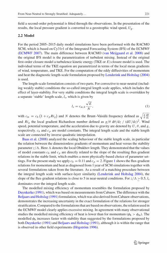
Baas et al. (2008) analyzed the scaling behaviour of the stable length scale, in particularthe relation between the dimensionless gradients of momentum and heat versus the stabilityparameter z/�. Here� denotes the local Obukhov length. They demonstrated that the valuesof model constants ch and cp are directly related to the slope of the resulting flux-gradientrelations in the stable limit, which enables a more physically-based choice of parameter set-tings. For the present study we apply ch = 0.11 and cp = 2. Figure 1 shows the flux-gradientrelations for momentum and heat as diagnosed from 1year of SCM simulations together withseveral formulations taken from the literature. As a result of a matching procedure betweenthe integral length scale with surface-layer similarity (Lenderink and Holtslag 2004), theslope of the flux-gradient relations is close to 5 in near-neutral conditions. For z/�>∼ 0.5, lsdominates over the integral length scale.

The modelled mixing efficiency of momentum resembles the formulation proposed byDuynkerke (1991), which was based onmeasurements fromCabauw. The difference with theBeljaars andHoltslag (1991) formulation,whichwas also derived fromCabauwobservations,demonstrates the increasing uncertainty in the exact formulation of the relations for strongerstratification.Compared to the formulations that are basedonobservations, the relationused inthe ECMWFmodel clearly applies excessive mixing. In agreement with many observationalstudies the modelled mixing efficiency of heat is lower than for momentum (φh > φm). Themodelled φh increases faster with stability than suggested by the formulations proposed byboth Duynkerke (1991) and Beljaars and Holtslag (1991), although it is within the range thatis observed in other field experiments (Högström 1996).

123

222 P. Baas et al.

Fig. 1 Dimensionless gradients of wind, ϕm , and temperature, ϕh , as a function of the local stability parameterz/� as diagnosed from 1year of model output (grey dots). Red lines indicate 1 + 5 z/� (Dyer 1974), greenlines the Beljaars and Holtslag (1991) formulation, blue lines the relations proposed by Duynkerke (1991),and yellow lines the formulation that is used in the ECMWF model

It is interesting to compare the present results to idealized simulations performed by e.g.van de Wiel et al. (2008) and Ansorge and Mellado (2014). Those studies investigated aca-demic, fully homogeneous and stationary flow, using direct numerical simulations and foundstrong support for the log-linear (Businger–Dyer) relations. However, it must be realizedthat turbulent mixing schemes in current realistic models are also supposed to representthe effect of, for example, surface heterogeneity (McCabe and Brown 2007), intermittentturbulence (van de Wiel et al. 2002), and gravity waves (Steeneveld et al. 2008). The sameprocesses explain why virtually all observational studies on flux-gradient relations report thatfor increasing stability the exchange of momentum is far more efficient than the exchangeof heat, i.e. φh > φm (Beljaars and Holtslag 1991). This justifies additional mixing ofmomentum compared to results from idealized model studies (Delage 1997; Yagüe et al.2001).

This observationally-based increase of the mixing efficiency should not be confused withthe so-called ‘enhanced mixing’ (i.e. way beyond what is observed in field experiments) thatis frequently applied in operational models in order to optimize large-scale model scores(Viterbo et al. 1999).

Details of other components of the SCM can be found in ECMWF (2007). Radiationtransport is modelled with the Rapid Radiation TransferModel (RRTM) scheme. Interactionswith the surface and soil dynamics are represented by the Tiled ECMWF Scheme for SurfaceExchanges over Land (TESSEL) scheme, which consists of four layers in the soil, a ‘skinlayer’ with zero heat capacity, and a vegetation layer. Following Bosveld et al. (2014), weapply a roughness length of 0.15 m for momentum and 0.0015 m for heat.

The SCM simulations are forced with output from daily three-dimensional forecasts ofthe RACMO 2.1 model (van Meijgaard et al. 2008) starting at 1200 UTC from the ECMWFanalysis. The forcing data consist of initial profiles and time-height fields of the geostrophicwind, vertical velocity, and advective tendencies of wind, temperature and humidity.

The SCM simulations are initialized at 1200 UTC and the simulation time is 48h. Herewe use model output with a lead time of between +24 and +48h. No data assimilation ornudging to three-dimensional model fields is applied. The SCM grid consists of 90 verticallevels, and near the surface the grid spacing is roughly 6 m, with the lowest level locatedat approximately 3m above the surface. This high-resolution grid configuration is adoptedfrom the GABLS4 intercomparison study (E. Bazile, personal communication, 2017).

123

From Near-Neutral to Strongly Stratified: Adequately… 223

3 Classification

We classify 11years of observations and SCM simulations in terms of the horizontal pressuregradient, expressed as the geostrophic wind speed. As the scope of the present study is limitedto studying the response of the NBL dynamics to variations in mechanical forcing conditions,nights with overcast conditions were excluded from the analysis. To enable a comparisonbetween summertime and wintertime nights, all nights are synchronized by the moment thatthe net radiation, Qn, changes sign from positive to negative. Hereafter, we refer to thismoment as t = 0h or ‘the transition’.

To filter out nights with overcast conditions, only nights with an average Qn of less than− 30 W m−2 were selected. The average is taken over the period t = 0–8h. To avoid selectionof nights with large variations in cloudiness, the standard deviation of Qn within this periodis required to be less than half the modulus of the average value.

For each night, the ambientUg is calculated by taking the average between t = − 4 h andt = 8 h. To guarantee relatively constant values throughout the nights, only nights for whichthe standard deviation of Ug < 1.5 m s−1 are included in the analysis. Selected nights areclassified in terms of the average Ug using a bin-width of 1 m s−1.

The classification is done independently for both the model and the observations. Assuch, we rather compare nights with similar mechanical forcing conditions, than presentinga one-to-one comparison of observed and modelled nights. As we focus on comparing theobserved and modelled response of the NBL dynamics to a changing mechanical forcing thisis a legitimate approach. Also, in this way any discrepancies between the dynamical forcingsof the model simulations and the actual forcing conditions are avoided. Although the qualityof the model forcing data is generally reasonable (bias and root-mean-square error of themodelled Ug amounts to − 0.59 and 2.21 m s−1, respectively), only 21% of observed andmodelled nights are classified in the same bin of Ug. In 10% of the nights the difference isfour or more classes ofUg. These differences are a direct consequence of the small bin-widthof 1 m s−1 that we apply and the fact that we use model output with a +24 to +48h leadtime.

Table 1 indicates the number of nights for each class of Ug for both the observations andthe model. Clearly, although the selected bin-width is very small, for each class of Ug asignificant number of nights is present. Nights with a Ug value over 16 m s−1 are left out ofthe analysis due to the small number of nights within these classes.

4 Results

Here, the model results are compared to the observations. First, we present the results of theclassification in terms of Ug (Sect. 4.1). Observed and modelled ensemble-averaged time-series of turbulent fluxes and composite profiles of wind speed and potential temperature areshown. This provides valuable insights into the model performance for a gradual increase ofthe mechanical forcing of the boundary layer. Second, we explore to what extent the modelreproduces qualitatively different NBL regimes that have been distinguished in observations(Sect. 4.2). The results are related to recent conceptual findings. Third, the impact of turbulentmixing and the strength of the land-atmosphere coupling are studied by analyzing results ofidealized SCM simulations with increasing geostrophic wind speed (Sect. 4.3).

123

224 P. Baas et al.

Table 1 Number of observedand modelled nights for eachclass of Ug

Ug(m s−1) # Obs # Model

1–2 40 49

2–3 67 98

3–4 84 90

4–5 112 141

5–6 109 133

6–7 115 128

7–8 117 108

8–9 116 121

9–10 103 96

10–11 83 79

11–12 56 60

12–13 54 48

13–14 50 47

14–15 33 35

15–16 28 17

4.1 Classification in Terms of Geostrophic Wind

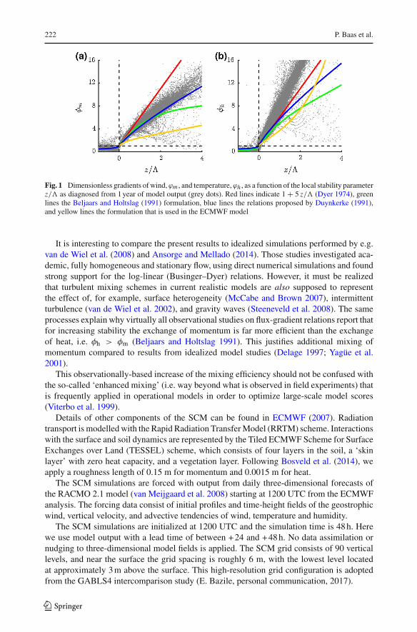
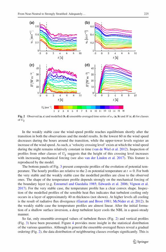
Figure 2 shows the ensemble-averaged course of the observed and modelled friction veloc-ity, u∗, and sensible heat flux, H . In general, the model reproduces the temporal evolutionof the fluxes and the dependence on Ug rather well. The magnitude of the fluxes increasesmonotonically with increasing Ug. Although the modelled turbulent fluxes are somewhatlarger than those observed, the general qualitative features appear to be similar to the obser-vations.

For the classes with lower Ug, the ensemble-averaged model results show a much lesspronounced maximum in H in the first two hours after the transition. On the other hand,inspection of individual days indicates that this feature is present in a substantial part ofthe modelled nights: for Ug ∈ [2, 3) m s−1, H decreases by more than half between themaximum just after the transition and t = 4 h in 44 % of the modelled nights (for theobservations this is the case in 84 % of the nights). The observed decrease of H over thecourse of the night (from t = 2–9h) is reproduced by the model. This trend is related to asimilar trend in Qn (not shown).

Figure 3 presents compositewind-speed and potential temperature profiles for two selectedclasses of Ug, representing typically very stable, Ug ∈ [2, 3) m s−1, and weakly stableconditions, Ug ∈ [14, 15) m s−1. For both classes, the evolution of the profiles is indicatedwith hourly intervals from 2 h prior to the transition to 9 h afterwards.

The upper panels of Fig. 3 present the evolution of the composite wind-speed profiles.In very stable conditions, the observations show a decrease of the wind speed below 40m in the hours prior to the transition. After the transition the wind-speed profile does notchange significantly during the entire night. No clear inertial oscillation nor an associatedlow-level jet occurs as the ageostrophic wind components are small. The modelled profilesare reasonably close to the observed ones from 2 h after the transition to the end of the night.However, during the transition and the preceding late-afternoon, the wind speeds in themodelare lower than observed.

123

From Near-Neutral to Strongly Stratified: Adequately… 225

Fig. 2 Observed (a, c) and modelled (b, d) ensemble-averaged time series of u∗ (a, b) and H (c, d) for classesof Ug

In the weakly stable case the wind-speed profile reaches equilibrium shortly after thetransition in both the observations and the model results. In the lowest 60 m the wind speeddecreases during the hours around the transition, while the upper-tower levels register anincrease of the wind speed. As such, a ‘velocity crossing level’ exists at which the wind speedduring the night remains relatively constant in time (van de Wiel et al. 2012). Inspection ofprofiles from other classes of Ug suggests that the height of this crossing level increaseswith increasing mechanical forcing (see also van der Linden et al. 2017). This feature isreproduced by the model.

The bottom panels of Fig. 3 present composite profiles of the evolution of potential tem-perature. The hourly profiles are relative to the 2-m potential temperature at t = 0. For boththe very stable and the weakly stable case the modelled profiles are close to the observedones. The shape of the temperature profile depends strongly on the mechanical forcing ofthe boundary layer (e.g. Estournel and Guedalia 1985; Edwards et al. 2006; Vignon et al.2017). For the very stable case, the temperature profile has a clear convex shape. Inspec-tion of the modelled profiles of the sensible heat flux indicates that turbulent cooling onlyoccurs in a layer of approximately 40 m thickness (not shown). At higher levels all coolingis the result of radiative flux divergence (Garratt and Brost 1981; McNider et al. 2012). Inthe weakly stable case the temperature profiles are almost linear. After the initial forma-tion of a shallow surface inversion, a deep turbulent layer cools the NBL in a quasi-steadymanner.

So far, only ensemble-averaged values of turbulent fluxes (Fig. 2) and vertical profiles(Fig. 3) have been presented. Figure 4 provides more insight in the statistical distributionof the various quantities. Although in general the ensemble-averaged fluxes reveal a gradualordering (Fig. 2), the data distribution of neighbouring classes overlaps significantly. This is

123

226 P. Baas et al.

Fig. 3 Hourly evolution of observed (Obs) andmodelled (SCM) composite profiles of wind speed (top panels)and potential temperature differences (bottom panels) for two classes of Ug from t = −2 − 9 h. a, b, e, fUg[2, 3) m s−1. c, d, g, hUg ∈ [14, 15) m s−1. Potential temperature differences are relative to the 2-m valueat t = 0. Colours indicate the time relative to the transition

shown in Fig. 4a, b, which presents the distribution of the turbulent fluxes for each class ofUg. The percentiles are based on data from the period t = 4–8 h after the transition. As canbe seen in Fig. 2, in this period the ensemble-averaged fluxes are relatively constant in time.Figure 4a, b shows that the modelled distributions within classes of Ug are reasonably closeto the observed ones.

Figure 4c, d presents the distribution of wind shear and stratification (200 m minus near-surface values) for each class of Ug. For both quantities the modelled distributions are veryclose to the observed ones over the full range ofUg classes. This may be an unexpected resultas the modelled turbulent fluxes are larger than those observed (Fig. 4a, b). However, witha roughness length that depends on wind direction and the presence of internal boundarylayers, the observational practice is much more complicated than the relatively simple modelenvironment. As such, no straightforward relation between the magnitude of the surfacefluxes and the shape of the vertical profiles exists.

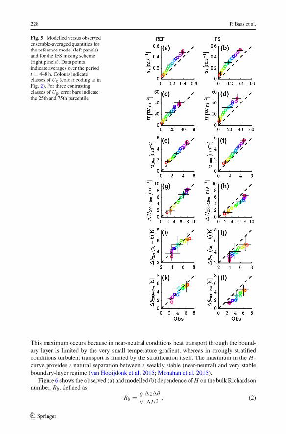
In Fig. 5, modelled ensemble-averages are compared directly to observed values for dif-ferent variables. Different colours indicate different classes of Ug. The data points representaverage values for the period t = 4–8 h after the transition. For comparison, the SCM simu-lations were repeated with the IFS mixing scheme (i.e. a first-order turbulent closure schemewith enhanced mixing). The results are included in Fig. 5.

Figure 5a, c confirms that the magnitude of the turbulent fluxes tends to be too large forthe reference model. As in Fig. 2, the ensemble-averaged fluxes show a gradual ordering asa function of Ug. However, as indicated by the error-bars, which indicate the 25th and 75th

123

From Near-Neutral to Strongly Stratified: Adequately… 227

Fig. 4 Observed (red) and modelled (blue) distributions of u∗ (a), H (b), wind shear (c), and stratification(d) for classes of Ug. Only data between t = 4 and t = 8 h are included. For each class, the symbol indicatesthe median value, the error bars the 25th and 75th percentiles, and the outer lines the 10th and 90th percentiles

percentiles, the overlap between subsequent classes is significant. The surface fluxes for theIFS mixing scheme are shown in Fig. 5b, d. In this case the overestimation of the surfacefluxes is larger than for the reference model.

The reference model slightly overestimates the 10-m wind speed for the whole range ofconsidered geostrophic wind speeds (Fig. 5e). Also the modelled wind shear between 200and 10 m above the surface is very close to the observed values (Fig. 5g). As a result ofthe vertical mixing being too intense, the IFS results show a larger overestimation of the10-m wind speed, in particular for the classes with highest Ug (Fig. 5f). The wind shear issystematically underestimated (Fig. 5h).

A comparable pattern emerges when considering temperature. Figure 5i, j shows thedecrease in θ2m since t = 0. Although the spread in the data is considerable, the referencemodel is reasonably close to the observations for the entire mechanical forcing range, whilethe IFS model underestimates the near-surface cooling. This is consistent with modelledvalues of the inversion strength, which are close to the observations for the reference modeland clearly too low for the IFS model (Fig. 5k, l). The present results agree with manyearlier studies reporting that the enhanced mixing applied in most global operational modelsis detrimental for the representation of the NBL (e.g. Cuxart et al. 2006; Brown et al. 2008;Sandu et al. 2013).

4.2 Nocturnal Boundary-Layer Regimes

Many authors have discussed the occurrence of a maximum in the magnitude of the sensibleheat flux for intermediate stratification (e.g. De Bruin 1994; Malhi 1995; Mahrt et al. 1998).

123

228 P. Baas et al.

Fig. 5 Modelled versus observedensemble-averaged quantities forthe reference model (left panels)and for the IFS mixing scheme(right panels). Data pointsindicate averages over the periodt = 4–8 h. Colours indicateclasses of Ug (colour coding as inFig. 2). For three contrastingclasses of Ug, error bars indicatethe 25th and 75th percentile

This maximum occurs because in near-neutral conditions heat transport through the bound-ary layer is limited by the very small temperature gradient, whereas in strongly-stratifiedconditions turbulent transport is limited by the stratification itself. The maximum in the H -curve provides a natural separation between a weakly stable (near-neutral) and very stableboundary-layer regime (van Hooijdonk et al. 2015; Monahan et al. 2015).

Figure 6 shows the observed (a) andmodelled (b) dependence of H on the bulk Richardsonnumber, Rb, defined as

Rb = g

θ

�z�θ

�U 2 , (2)

123

From Near-Neutral to Strongly Stratified: Adequately… 229

Fig. 6 Observed (a) andmodelled (b) relation between H and Rb. Colours indicate the number of occurrences.The dashed lines correspond to Rb = 0.04 and Rb = 1

with �z = 40 m, �θ is the potential temperature difference between 40 and 2 m and �Uis the 40-m wind speed. Figure 6 includes 10-min data from t = −4 to 9h for all selectednights. A clear maximum occurs for Rb ≈ 0.04 (indicated by a dashed line) for both theobservations and the model results. A second line is drawn at Rb = 1 and above this value,H is generally very small. In the following, we use those characteristic values of Rb as areference. We notice that the exact values have no general validity as they will be differentfor varying definitions of Rb.

In agreement with the results of Monahan et al. (2015), the data density peaks in thedescending branch of the H -curve for both the observations and the model results (Fig. 6).At first sight, this may be counter-intuitive as larger gradients lead to smaller turbulent fluxes,leading to even stronger gradients until all turbulence has disappeared (positive feedback).Therefore, it has been argued that this descending branch is dynamically unstable and wouldtherefore occur less frequently in nature. This apparent contradiction has been solved recentlyby van de Wiel et al. (2017). They showed that in reality negative feedbacks in soil heattransfer and radiation often overrule the aforementioned feedback in the turbulent heat flux.As a result, the formation of stronger and stronger inversions is counteracted. In fact, trueinstability of the descending branch is only possible over strongly isolating surfaces suchas fresh snow or in idealized model simulations where the negative feedback in soil heattransport and radiation is not taken into account. For instance, this occurs when the surfacecooling is forced by a fixed heat extraction (e.g. Donda et al. 2015; van Hooijdonk et al.2017).

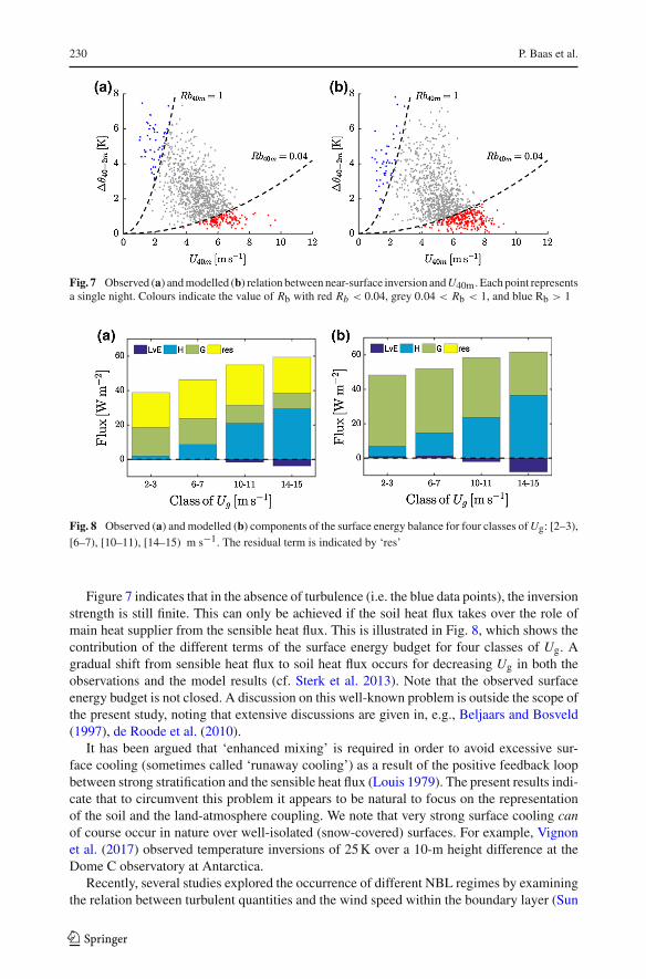
Following van de Wiel et al. (2017), we analyze the inversion strength of the lowest 40 m(�θ40−2m) as a function of the 40-m wind speed, U40m. Each data point in Fig. 7 representsa single night and is based on average values of the inversion strength andU40m between t =4–8 h after the transition. Colours indicate the relation with the H -curve (Fig. 6), with thered points indicating the ascending branch, the grey points the descending branch, and theblue points vanishing turbulence in strongly stratified conditions.

The overall relation between the inversion and the wind speed appears to be very similarbetween the observations (a) and the model results (b). For high 40-m wind speeds theinversion stays limited to approximately 1K. For intermediate wind speeds the inversionstrength increases rapidly for decreasing wind speed. As predicted by van de Wiel et al.(2017), the transition between these two regimes coincides with the maximum H -curve,indicated by a black-dashed line. The inversion strength is bound to a maximum, which isattained when the downward turbulent transport of warm air is completely suppressed. Thisoccurs for very weak winds.

123

230 P. Baas et al.

Fig. 7 Observed (a) andmodelled (b) relation betweennear-surface inversion andU40m.Each point representsa single night. Colours indicate the value of Rb with red Rb < 0.04, grey 0.04 < Rb < 1, and blue Rb > 1

Fig. 8 Observed (a) and modelled (b) components of the surface energy balance for four classes ofUg: [2–3),[6–7), [10–11), [14–15) m s−1. The residual term is indicated by ‘res’

Figure 7 indicates that in the absence of turbulence (i.e. the blue data points), the inversionstrength is still finite. This can only be achieved if the soil heat flux takes over the role ofmain heat supplier from the sensible heat flux. This is illustrated in Fig. 8, which shows thecontribution of the different terms of the surface energy budget for four classes of Ug. Agradual shift from sensible heat flux to soil heat flux occurs for decreasing Ug in both theobservations and the model results (cf. Sterk et al. 2013). Note that the observed surfaceenergy budget is not closed. A discussion on this well-known problem is outside the scope ofthe present study, noting that extensive discussions are given in, e.g., Beljaars and Bosveld(1997), de Roode et al. (2010).

It has been argued that ‘enhanced mixing’ is required in order to avoid excessive sur-face cooling (sometimes called ‘runaway cooling’) as a result of the positive feedback loopbetween strong stratification and the sensible heat flux (Louis 1979). The present results indi-cate that to circumvent this problem it appears to be natural to focus on the representationof the soil and the land-atmosphere coupling. We note that very strong surface cooling canof course occur in nature over well-isolated (snow-covered) surfaces. For example, Vignonet al. (2017) observed temperature inversions of 25K over a 10-m height difference at theDome C observatory at Antarctica.

Recently, several studies explored the occurrence of different NBL regimes by examiningthe relation between turbulent quantities and the wind speed within the boundary layer (Sun

123

From Near-Neutral to Strongly Stratified: Adequately… 231

Fig. 9 Modelled (top panels) and observed (bottom panels) u∗ and H versus Ug and U40m. Black plusesindicate ensemble-averaged values for the different classes of Ug. Colours indicate the value of Rb with redRb < 0.04, grey 0.04 < Rb ≤ 1, and blue Rb > 1

et al. 2012, 2016; van de Wiel et al. 2012; Acevedo et al. 2015; Vignon et al. 2017). Inview of these studies, in Fig. 9 we plot u∗ and H versus Ug (external mechanical forcing)and U40m (internal parameter) for both the observations and the model results. Each datapoint represents average values over t = 4–8h for a single night. Again, the colours indicatethe relation to the H -curve. (Note that for u∗ we prefer the local friction velocity (i.e. theeddy-covariance value, see Sect. 2.1) as we now focus on the internal NBL dynamics andnot on a direct comparison with model values).

Figure 9a, c indicate that the modelled u∗ and H increase linearly with Ug; the class-averaged values are nearly on a straight line that crosses the origin. There is no sign of atransition between regimes. The observed dependence of u∗ and H on Ug, is not as linearas for the model results (Fig. 9e, g), but still a possible transition between regimes is muchmore gradual than when the fluxes are related to a wind speed within the boundary layer.The present results resemble those of McNider et al. (2012), who ran their SCM for a broadrange of geostrophic wind speeds.

When plotting u∗ and H versusU40m, a clear ‘hockey stick transition’ emerges as reportedbefore by various authors (Sun et al. 2012, 2016; van de Wiel et al. 2012; van Hooijdonket al. 2015). The relations produced by the model are close to the observed ones, at least in aqualitative way. The ‘kink’ in the hockey sticks coincides with the value of Rb above whichturbulence is weak. The maximum in the H -curve occurs for much larger wind speeds.

The question remains why the transition from very stable to weakly stable conditionsis much more gradual from the perspective of Ug than from the perspective of U40m. Wesuggest that the difference between the two has its origin in a non-linear relation betweenUg

andU40m. Model results indicate that for strong stratification the top of the turbulent layer isclose to the 40-m level. As a result, in this case U40m is prone to inertial accelerations. Fornear-neutral conditions the turbulent layer is much deeper than 40 m. Consequently, U40m

will be substantially reduced by flux divergence.

123

232 P. Baas et al.

4.3 Idealized Model Simulations

It has been shown (Fig. 8) that in strongly-stratified conditions the radiative loss at the surfaceis largely compensated for by the soil heat flux. For these conditions the inversion strength ismainly determined by the strength of the land-atmosphere coupling (Sterk et al. 2013;Bosveldet al. 2014; van de Wiel et al. 2017). Unfortunately, the representation of soil and vegetationprocesses is complex and involves many uncertain parameters, especially on a spatial scale.Here, we demonstrate the impact of the strength of the land-atmosphere coupling on themodelled inversion strength.

To this end, we defined an idealized model experiment that was run with two different val-ues of the skin-layer conductivity. The reference value used in the model is 10 W m−2 K−1,which is a reasonable value for a grassland site such as Cabauw (van den Hurk and Beljaars1996). As a sensitivity experiment, the reference value was divided by 5. This is probablynot realistic for Cabauw, but serves as an illustration for very weak land-atmosphere cou-pling, for instance in the presence of snow cover. The two permutations were run with boththe reference model and the IFS mixing scheme. For each combination of skin conductiv-ity and turbulence scheme, nine simulations were performed with a gradually increasinggeostrophic wind speed (0.1, 2, 4, 6, 8, 10, 12, 16, 24 m s−1). Due to the idealized modelset-up a direct comparison with the results of the realistic simulations is not straightforward.For instance, the specific humidity was set to very low values to prevent cloud formationleading to increased surface (radiative) cooling rates.

Figure 10 shows the temperature difference between 40 m and the surface as a functionof U40m. For each of the simulations, average values over the period t = 4–8h are plotted.For large Ug, differences between the four sets of simulations are small. For vanishing Ug

the inversion strength is almost entirely determined by the strength of the surface couplingand differences between the two vertical-mixing schemes are small. In these conditionsturbulence is weak, even in the simulations that apply enhanced mixing. For moderate Ug

large differences exist between the two turbulence schemes with weaker inversions and lesswind shear in the enhanced mixing simulations.

We note that the temperature difference between 40 and 2m shows non-linear behaviourfor vanishing mechanical forcing: below a certain threshold value the inversion strengthincreases again for decreasing geostrophic forcing (not shown). This phenomenon that thenear-surface temperature increases when the wind speed becomes very small is discussedextensively in McNider et al. (2012) and Sterk et al. (2013).

Fig. 10 Temperature differencebetween 40 m and the surfaceversus U40 for idealized SCMsimulations. The reference modelis indicated in red, the IFS modelin blue. Diamonds indicatereference model settings,plus-signs reduced skin-layerconductivity. Each modelconfiguration is run for a suite ofnine geostrophic wind speeds

123

From Near-Neutral to Strongly Stratified: Adequately… 233

5 Discussion

The present results indicate that NWPmodels should in principle be able to represent theNBLin a satisfactory way. That is to say, for a wide range of mechanical forcing conditions theyshould be able to reproduce observed temperature inversions, wind shear, and near-surfaceparameters with reasonable accuracy (cf. Steeneveld et al. 2006; Sterk et al. 2015).

However, this is in contrast with the general opinion that atmospheric models are not ableto represent (strongly) stably-stratified conditions satisfactorily. We explain this as follows.Although turbulence mixing is indeed complex and highly uncertain under strongly-stratifiedconditions, its absolute contribution to the thermodynamic balance of the boundary layerbecomes significantly smaller as the wind speed decreases (Fig. 8). The same holds for themagnitude of the turbulent stresses, which become relatively less important in relation to theother terms in the moment equation. At the same time, we recognize that, given the largevertical gradients in temperature and wind speed, small changes in the model’s mixing prop-erties will have a significant impact on the shape of the profiles and the value of near-surfaceparameters.

Turbulence parametrizations have often been designed for idealized, homogeneous tur-bulence, while in model practice they are also supposed to account for patchy, intermittentturbulence. They are even supposed to include the effect of terrain inhomogeneities and/orprocesses they were never designed for, like (small-scale) gravity-wave drag. The complexityof processes that are responsible for vertical mixing contributes significantly to the modellingproblem of the SBL. On the other hand, the fact that leading large-scale models deliberately,albeit for defensible reasons, degenerate the quality of the vertical-mixing parametrizationby increasing the mixing efficiency to unrealistic amounts, has in our opinion obscured thediscussion of model performance in stably-stratified conditions.

A proper representation of land-atmosphere interactions is key to the realistic modellingof stably-stratified conditions. As demonstrated in the present study, this is particularly truefor very stable conditions. Unfortunately, parameters that govern the dynamics of the soiland vegetation are often highly uncertain. Moreover, the spatial variability in land cover, thecomposition of the soil, and the impact of soil moisture are usually enormous.

Taking into account all the complexities of modelling stably-stratified conditions, thechallenge of the present study is relatively straightforward. In an SCM setting, the role ofspatial variability is minimal (it is not completely absent as, for example, the actual roughnesslength depends on the wind direction). As such, it is, for example, not guaranteed that thepresent settings of the vertical-mixing scheme and the representation of the land-atmosphereinteractions will yield equally good results for locations with contrasting surface characteris-tics or different climates. Still, the current results indicate that the physical parametrizationsin large-scale models are in principle sufficiently equipped for modelling stably-stratifiedconditions for a wide range of forcing conditions.

Finally, we notice that in this study we apply a vertical resolution that is much higher thanwhat is typically used in operational practice (approximately 6 m in the lowest 100 m). Twoexperiments with coarser grid spacing were performed to study the impact of resolution onthe results. The impact of the resolution on the ensemble-averaged wind speed and temper-ature profiles proved to be small. This is shown in the Appendix, which presents compositetemperature profiles for two contrasting classes ofUg. It appears that temperatures at the gridlevels are close to each other, while differences inmodelled surface temperatures are small. Ofcourse, for individual cases features such as low-level jets and sharp inversions aremuchbetter

123

234 P. Baas et al.

resolved with a fine grid configuration. Although a comprehensive analysis on the impact ofvertical resolution would be interesting in itself, it falls beyond the scope of the present study.

6 Conclusions

The present work systematically evaluates the performance of an atmospheric single-columnmodel (SCM) for stably-stratified conditions. In particular, the modelled response of theclear-sky nocturnal boundary layer (NBL) dynamics to changing mechanical forcing con-ditions is investigated using observations from the Cabauw observatory, The Netherlands,as a reference. Therefore, 11years of model simulations and observations are selected onclear nights and classified in terms of the ambient geostrophic wind speed. The long datasetallows for a small bin-width of only 1 m s−1, which provides a detailed picture of the model’sperformance for a broad range of stability conditions, ranging from near-neutral to stronglystratified.

A comparison ofmodelled and observed ensemble-averaged time series of turbulent fluxesand vertical profiles of wind speed and temperature demonstrates that the model representsthe dynamics of the NBL at Cabauw very well for a broad range of mechanical forcingconditions. The model responds realistically to changing mechanical forcing conditions. Themodel performs well in both near-neutral (weakly stable) and strongly-stratified (very stable)conditions. Observed NBL regime transitions are represented in a natural way. The modelresembles characteristics of several conceptual models that study the occurrence of multipleregimes.

The reference model version performs much better than a model version that appliesexcessive vertical mixing as is applied in several (global) operational models. The detrimen-tal impact of this ‘enhanced mixing’ is obvious for the entire range of considered forcingconditions. The difference between the two model versions illustrates that, on the one hand,NWP models are in principle able to reproduce the NBL for a wide variety of stability con-ditions but that, on the other hand, in operational practice the interactions between the NBLand other model aspects are still not well understood.

For strongly-stratified conditions, turbulent fluxes constitute only a small fraction of thesurface energy budget. In other words, for these conditions the radiative loss at the surfaceis largely balanced by the soil heat flux. Model sensitivity runs showed that for weak-windconditions the inversion strength depends much more on details of the land-atmospherecoupling than on the turbulent mixing. The impact of the turbulence scheme is largest formoderate stability.

The presented results indicate that NWPmodels are in principle able to represent the NBLsatisfactorily for a wide range of mechanical forcing conditions. Further research shouldelucidate whether this conclusion holds for conditions with much weaker land-atmospherecoupling like snow-covered areas or ice-sheets.

Acknowledgements We thank Erik van Meijgaard (KNMI) for providing the three-dimensional forcing datafor driving the single-column model. Three anonymous reviewers are acknowledged for their constructivecomments. We gratefully acknowledge funding by a Consolidator Grant from the European Research Council(648666).

Open Access This article is distributed under the terms of the Creative Commons Attribution 4.0 Interna-tional License (http://creativecommons.org/licenses/by/4.0/), which permits unrestricted use, distribution, andreproduction in any medium, provided you give appropriate credit to the original author(s) and the source,provide a link to the Creative Commons license, and indicate if changes were made.

123

From Near-Neutral to Strongly Stratified: Adequately… 235

Fig. 11 Ensemble-averaged vertical profiles of potential temperature for two classes ofUg: a [2,3) b [14,15)for the observations (black), the reference model (red), the 91 levels (green) and the 31 levels configuration(blue). Markers indicate model levels. For the three model versions the surface temperature is included as well

Appendix

To assess the sensitivity of the results to vertical resolution of the SCM, two sets of simu-lations with reduced resolution were performed. The first had the lowest five grid levels atapproximately 10, 34, 67, 111, and 166m. The second is a very coarse 31-layer configurationwith the lowest grid levels at 32, 147, and 350m. Simulation period (2005–2015), modelphysics, and classification procedure were equal to those of the reference results. Figure 11presents ensemble-averaged temperature profiles for two contrasting classes ofUg. From thiscomposite perspective the impact of the enormous differences in resolution are small as thevalues at the grid levels are close to each other. Also the modelled surface temperatures areremarkably close.

References

Acevedo OC, Mahrt L, Puhales FS, Costa FD, Medeiros LE, Degrazia GA (2015) Contrasting structuresbetween the decoupled and coupled states of the stable boundary layer. Q J RMeteorol Soc 142:693–702

Ansorge C, Mellado JP (2014) Global intermittency and collapsing turbulence in the stratified planetaryboundary layer. Boundary-Layer Meteorol 153:89–116

Atlaskin E, Vihma T (2012) Evaluation of NWP results for wintertime nocturnal boundary-layer temperaturesover Europe and Finland. Q J R Meteorol Soc 138:1440–1451

Baas P, de Roode SR, Lenderink G (2008) The scaling behaviour of a turbulent kinetic energy closure modelfor stably stratified conditions. Boundary-Layer Meteorol 127:17–36

Baas P, Bosveld FC, van LenderinkG,Meijgaard E,HoltslagAAM (2010)How to design single-columnmodelexperiments for comparison with observed nocturnal low-level jets. Q J R Meteorol Soc 136:671–684

Banta RM, Newsom RK, Lundquist JK, Pichugina YL, Coulter RL, Mahrt L (2002) Nocturnal low-level jetcharacteristics over Kansas during CASES-99. Boundary-Layer Meteorol 105:221–252

Beare R (2007) Boundary layer mechanism in extra tropical cyclones. Q J R Meteorol Soc 133:503–515Beljaars ACM (1982) The derivation of fluxes from profiles in perturbed areas. Boundary-Layer Meteorol

24:35–55Beljaars ACM, Holtslag AAM (1991) Flux parameterization over land surfaces for atmospheric models. J

Appl Meteorol 30:327–341Beljaars ACM, Bosveld FC (1997) Cabauw data for the validation of land surface parameterization schemes.

J Clim 10:1172–1193Bosveld FC, Beyrich F (2004) Classifying observations of stable boundary layers for model validation. In: Pro-

ceedings of 16th symposium on boundary layers and turbulence, Portland,ME.AmericanMeteorologicalSociety, P4.13

123

236 P. Baas et al.

Bosveld FC, Baas P, SteeneveldGJ, HoltslagAAM,AngevineWM,Bazile E, deBruijn EIF, DeacuD, EdwardsJM, Ek M, Larson VE, Pleim JE, Raschendorfer M, Svensson G (2014) The third GABLS intercom-parison case for evaluation studies of boundary-layer models. Part B: results and process understanding.Boundary-Layer Meteorol 152:157–187

Brown A, Beljaars A, Hersbach H, Hollingsworth A, Miller M, Vasiljevic D (2005) Wind turning across themarine atmospheric boundary layer. Q J R Meteorol Soc 131:1233–1250

Brown A, Beare RJ, Edwards JM, Lock AP, Keogh SJ, Milton SF, Walters DN (2008) Upgrades to theboundary-layer scheme in the met office numerical weather prediction model. Boundary-Layer Meteorol128:117–132

Chimonas G, Nappo CJ (1989) Wave drag in the planetary boundary layer over complex terrain. Boundary-Layer Meteorol 47:217–232

Cuxart J, Holtslag AAM, Beare RJ, Bazile E, Beljaars A, Cheng A, Conangla L, Ek MB, Freedman F,Hamdi R, Kerstein A, Kitagawa H, Lenderink G, Lewellen G, Mailhot J, Mauritsen T, Perov V, SchayesG, Steeneveld GJ, Svensson G, Taylor P, Weng W, Wunsch S, Xu KM (2006) Single-column modelintercomparison for a stably stratified atmospheric boundary layer. Boundary-Layer Meteorol 118:273–303

de Bruin HAR (1994) Analytic solutions of the equations governing the temperature fluctuation method.Boundary-Layer Meteorol 68:427–432

de Roode SR, Bosveld FC, Kroon PS (2010) Dew formation, eddy-correlation latent heat fluxes, and thesurface energy imbalance at Cabauw during stable conditions. Boundary-Layer Meteorol 135:369–383

Delage Y (1997) Parameterizing sub-grid scale vertical transport in atmospheric models under statically stableconditions. Boundary-Layer Meteorol 82:23–48

Donda JMM, van deWiel BJH,Bosveld FC,Beyrich F, vanHeijst GJF, ClercxHJH (2013) Predicting nocturnalwind and temperature profiles based on external forcing parameters. Boundary-LayerMeteorol 146:103–117

Donda J, van Hooijdonk I, Moene A, Jonker H, van Heijst G, Clercx H, van de Wiel B (2015) Collapse ofturbulence in stably stratified channel flow: a transient phenomenon. Q J RMeteorol Soc 141:2137–2147

Duynkerke PG (1991) Radiation fog: a comparison of model simulation with detailed observations. MonWeather Rev 119:324–341

Dyer AJ (1974) A review of flux-profile relationships. Boundary-Layer Meteorol 7:363–372ECMWF (2007) IFS documentation—Cy31r1. Part IV physical processes, ECMWF, Reading, UK, 155 ppEdwards JM (2009) Radiative processes in the stable boundary layer: part II. The development of the nocturnal

boundary layer. Boundary-Layer Meteorol 131:127–146Edwards JM, Beare RJ, Lapworth AJ (2006) Simulation of the observed evening transition and nocturnal

boundary layers: single column modelling. Q J R Meteorol Soc 132:61–80Estournel C, Guedalia D (1985) Influence of geostrophic wind on atmospheric nocturnal cooling. J Atmos Sci

42:2695–2698Fernando HJS, Weil JC (2010) Whither the stable boundary layer? A shift in the research agenda. Bull Am

Meteorol Soc 91:1475–1484Garratt JR, Brost A (1981) Radiative cooling effects within and above the nocturnal boundary layer. J Atmos

Sci 38:2730–2746Grachev AA, Fairall CW, Persson POG, Andreas EL, Guest PS (2005) Stable boundary layer scaling regimes:

the SHEBA data. Boundary-Layer Meteorol 116:201–235Högström U (1996) Review of some basic characteristics of the atmospheric surface layer. Boundary-Layer

Meteorol 78:215–246Holtslag AAM, Svensson G, Baas P, Basu S, Beare B, Beljaars ACM, Bosveld FC, Cuxart J, Lindvall J,

Steeneveld GJ, Tjernström M, van de Wiel BJH (2013) Stable atmospheric boundary layers and diurnalcycles—challenges for weather and climate models. Bull Am Meteorol Soc 94:1691–1706

Lenderink G, Holtslag AAM (2004) An updated length-scale formulation for turbulent mixing in clear andcloudy boundary layers. Q J R Meteorol Soc 130:3405–3427

Louis JF (1979) A parametric model of vertical eddy fluxes in the atmosphere. Boundary-Layer Meteorol17:187–202

Mahrt L, Sun J, Blumen W, Delany W, Oncley S (1998) Nocturnal boundary layer regimes. Boundary-LayerMeteorol 88:255–278

Mahrt L, Sun J, Stauffer D (2015) Dependence of turbulent velocities on wind speed and stratification.Boundary-Layer Meteorol 155:55–71

Malhi YS (1995) The significance of the diurnal solutions for heat fluxes measured by the temperature fluc-tuation method in stable conditions. Boundary-Layer Meteorol 74:389–396

Mauritsen T, Svensson G (2007) Observations of stably stratified shear-driven atmospheric turbulence at lowand high Richardson numbers. J Atmos Sci 64:645–655

123

From Near-Neutral to Strongly Stratified: Adequately… 237

McCabe A, Brown AR (2007) The role of surface heterogeneity in modelling the stable boundary layer.Boundary-Layer Meteorol 122:517–534

McNider RT, Steeneveld GJ, Holtslag AAM, Pielke RA Sr, Mackaro S, Pour-Biazar A, Walters J, Nair U,Christy J (2012) Response and sensitivity of the nocturnal boundary layer overland to added longwaveradiative forcing. J Geophys Res 117:D14106

Monahan AH, Rees T, He Y, McFarlane N (2015) Multiple regimes of wind, stratification, and turbulence inthe stable boundary layer. J Atmos Sci 72:3178–3198

MonnaW,Bosveld F (2013) In higher spheres—40 years of observations at theCabauw site. KNMIPublication232, De Bilt, The Netherlands, 56 pp

Neggers RAJ, Siebesma AP, Heus T (2012) Continuous single-column model evaluation at a permanentmeteorological supersite. Bull Am Meteorol Soc 93:1389–1400

Optis M, Monahan A, Bosveld FC (2015) Limitations and breakdown of Monin–Obukhov similarity theoryfor wind profile extrapolation under stable stratification. Wind Energy 19:1053–1072

Pithan F, Ackerman A, Angevine WM, Hartung K, Ickes L, Kelley M, Medeiros B, Sandu I, Steeneveld GJ,Sterk HAM, Svensson G, Vaillancourt PA, Zadra A (2016) Select strength and biases of models in repre-senting Arctic winter boundary layer over sea ice: the Larcform 1 single column model intercomparison.J Adv Model Earth Syst 8:1345–1357

Román-Cascón C, Steeneveld GJ, Yagüe C, Sastre M, Arrillaga JA, Maqueda G (2016) Forecasting radiationfog at climatologically contrasting sites: evaluation of statistical methods and WRF. Q J R Meteorol Soc142:1048–1063

Sandu I, Beljaars A, Bechtold P, Mauritsen T, Balsamo G (2013) Why is it so difficult to represent stablystratified conditions in numerical weather prediction (NWP) models? J Adv Model Earth Syst 5:117–133

Steeneveld GJ, van de Wiel BJH, Holtslag AAM (2006) Modeling the evolution of the atmospheric boundarylayer coupled to the land surface for three contrasting nights in CASES-99. J Atmos Sci 63:920–935

Steeneveld GJ, Holtslag AAM, Nappo CJ, van de Wiel BJH, Mahrt L (2008) Exploring the possible role ofsmall-scale terrain drag on stable boundary layers over land. J Appl Meteorol Clim 47:518–2530

Sterk HAM, Steeneveld GJ, Holtslag AAM (2013) The role of snow-surface coupling, radiation, and turbulentmixing in modeling a stable boundary layer over Arctic sea ice. J Geophys Res Atmos 118:1199–1217

Sterk HAM, Steeneveld GJ, Vihma T, Anderson PS, Bosveld FC, Holtslag AAM (2015) Clear-sky stableboundary layers with low winds over snow-covered surfaces. Part 1: WRF model evaluation. Q J RMeteorol Soc 141:2165–2184

Sun J, Mahrt L, Banta RM, Pichugina YL (2012) Turbulence regimes and turbulence intermittency in thestable boundary layer during CASES-99. J Atmos Sci 69:338–351

Sun J, Lenschow DH, LeMone MA, Mahrt L (2016) The role of large-coherent-eddy transport in the atmo-spheric surface layer based on CASES-99 observations. Boundary-Layer Meteorol 160:83–111

SvenssonG, Holtslag A (2009) Analysis of model results for the turning of the wind and the relatedmomentumfluxes and depth of the stable boundary layer. Boundary-Layer Meteorol 132:261–277

Svensson G, Holtslag AAM, Kumar V, Mauritsen T, Steeneveld GJ, Angevine WM, Bazile E, Beljaars A, deBruijn EIF, Cheng A, Conangla L, Cuxart J, Ek M, Falk MJ, Freedman F, Kitagawa H, Larson VE, LockA, Mailhot J, Masson V, Park S, Pleim J, Söderberg S, Weng W, Zampieri M (2011) Evaluation of thediurnal cycle in the atmospheric boundary layer over land as represented by a variety of single-columnmodels: the second GABLS experiment. Boundary-Layer Meteorol 140:177–206

Tsiringakis A, Steeneveld GJ, Holtslag AAM (2017) Small-scale orographic gravity wave drag in stableboundary layers and its impact on synoptic systems and near-surface meteorology. Q J R Meteorol Soc143:1504–1516

vanHooijdonk IGS,Donda JMM,Clercx JH,Bosveld FC, van deWielBJH (2015) Shear capacity as prognosticfor nocturnal boundary layer regimes. J Atmos Sci 72:1518–1532

van Hooijdonk IGS, Moene AF, Scheffer M, Clercx HJH, van de Wiel BJH (2017) Early warning signals forregime transition in the stable boundary layer: a model study. Boundary-Layer Meteorol 162:283–306

van den Hurk BJJM, Beljaars ACM (1996) Impact of some simplifying assumptions in the new ECMWFsurface scheme. J Appl Meteorol 35:1333–1343

van der Linden SJA, Baas P, van Hooft JA, van Hooijdonk IGS, Bosveld FC, van de Wiel BJH (2017) Localcharacteristics of the nocturnal boundary layer in response to external pressure forcing. J Appl MeteorolClim. doi:10.1175/JAMC-D-17-0011.1

van Meijgaard E, van Ulft LH, van de Berg WJ, Bosveld FC, van den Hurk BJJM, Lenderink G, SiebesmaAP (2008) The KNMI regional atmospheric climate model RACMO version 2.1. KNMI technical report302, De Bilt, The Netherlands, 43 pp

van Ulden AP, Wieringa J (1996) Atmospheric boundary layer research at Cabauw. Boundary-Layer Meteorol78:39–69

123

238 P. Baas et al.

van de Wiel BJH, Ronda RJ, Moene AF, de Bruin HAR, Holtslag AAM (2002) Intermittent turbulence andoscillations in the stable boundary layer over land. Part I: a bulk model. J Atmos Sci 59:942–958

van de Wiel BJH, Moene AF, De Ronde WH, Jonker HJJ (2008) Local similarity in the stable boundary layerand mixing-length approaches: consistency of concepts. Boundary-Layer Meteorol 128:103–116

van de Wiel BJH, Moene AF, Jonker HJJ, Baas P, Basu S, Donda JMM, Sun J, Holtslag AAM (2012) Theminimum wind speed for sustainable turbulence in the nocturnal boundary layer. J Atmos Sci 69:3116–3127

van de Wiel BJH, Vignon E, Baas P, van Hooijkdonk IGS, van der Linden SJA, van Hooft JA, Bosveld FC,de Roode SR, Moene AF, Genthon C (2017) Regime transitions in near-surface temperature inversions:a conceptual model. J Atmos Sci 74:1057–1073

Verkaik JW,HoltslagAAM(2007)Windprofiles,momentumfluxes and roughness lengths atCabauw revisited.Boundary-Layer Meteorol 122:701–719

Vignon E, van deWiel BJH, vanHooijdonk IGS, GenthonC, van der Linden SJA, vanHooft JA, Baas P,MaurelW, Traullé O, Casasanta G (2017) Stable boundary layer regimes at dome C, Antarctica: observation andanalysis. Q J R Meteorol Soc 143:1241–1253

Viterbo P, Beljaars A,Mahfouf JF, Teixeira J (1999) The representation of soil moisture freezing and its impacton the stable boundary layer. Q J R Meteorol Soc 125:2401–2426

Yagüe C, Maqueda G, Rees JM (2001) Characteristics of turbulence in the lower atmosphere at Halley IVstation, Antarctica. Dyn Atmos Oceans 34:205–223

123