1

High Time Resolution Astrophysics andPulsars

Andy Shearer1

National University of Ireland, Galway andy.shearer@nuigalway.ie

Summary. The discovery of pulsars in 1968 heralded an era where the temporalcharacteristics of detectors had to be reassessed. Up to this point detector integrationtimes would normally be measured in minutes rather seconds and definitely noton sub-second time scales. At the start of the 21st century pulsar observationsare still pushing the limits of detector/telescope capabilities. Flux variations ontimes scales less than 1 nsec have been observed during giant radio pulses. Pulsarstudies over the next 10–20 years will require instruments with time resolutions downto microseconds and below, high-quantum quantum efficiency, reasonable energyresolution and sensitive to circular and linear polarisation of stochastic signals. Thischapter is review of temporally resolved optical observations of pulsars. It concludeswith estimates of the observability of pulsars with both existing telescopes and intothe ELT era.

1.1 Introduction

Traditionally astrophysics has concerned itself with minimum time-scales mea-sured in hours rather than seconds. This was understandable as the availablerecording media were slow — e.g. chart recorders and photographic plates.In the 1950s, 60s and 70s wavebands away from the optical were developed— from ground based radio studies to space and balloon borne high energywork. In contrast to optical wavelengths instrumentation in these (high andlow energy) regimes was capable of time resolutions of less than a second.Vacuum tube and CCD technologies in the 1970s and 80s extended electronicdetectors to the optical band pass thereby allowing for studies, in the opti-cal regime, at all time scales. More recently superconducting detectors andavalanche photodiodes (APD) have given us the possibility of nanosecondobservations with high quantum efficiency. To date high time resolution ob-servations, in optical astronomy, have been driven predominantly by detectordevelopments and possibilities — and not by the underlying science. Thissituation is now changing where studies of stochastic phenomena such as gi-ant radio pulses (GRP) and rotating radio transients (RRAT) require specific

arX

iv:0

801.

0314

v1 [

astr

o-ph

] 1

Jan

200

8

2 Andy Shearer

types of detector and instrumentation. Table 1.1 shows the characteristic time-scale for different astronomical objects. Clearly studies of pulsars require theability to observe down to sub-millisecond and in some cases sub-microsecondtimes scales. Consequently, optical observations of pulsars probably representthe biggest instrumental challenge to high-time resolution astrophysics. Ra-dio observations [1] have shown flux variations from the Crab during GRPson time scales of nanoseconds. Although over 1600 radio pulsars have beenobserved, only five normal pulsars and one anomalous X-ray pulsar (AXP)have been observed to pulse at optical wavelengths. Optical observations ofpulsars are also limited by their intrinsic faintness in the optical regime seeTable 2.

Table 1.1. Small Timescale Variability of Astronomical Objects. Pulsars can beshown to require observations on the shortest time-scales - variability in the radioregion has been shown down to nanosecond scales and in the optical variability atthe microsecond scale has been observed.

Time-scale(now) (ELT era)

Stellar flares Seconds / 10–100 mspulsations Minutes

Stellar surface White Dwarfs 1–1000 µs 1–1000 µsoscillations Neutron Stars 0.1 µs

Close Binary Tomography 100 ms++ 10ms+Systems Eclipse in/egress 10 ms+ <1ms(accretion and Disk flickering 10 ms <1msturbulence ) Correlations 50 ms <1ms

(e.g. X & Optical)

Pulsars Magnetospheric 1 µs–100 ms ns(?)Thermal 10 ms <ms

AGN Minutes Seconds

In this chapter we present an analysis of optical observations of pulsarswhich have shown variability on time-scales from few nanoseconds to secularchanges over years. In this regard they represent the most challenging targetfor optical High-Time Resolution Astrophysics. Pulsars, neutron stars with anactive magnetosphere, are created through one of two main processes — thecompact core after a type II supernova explosion or as a result of accretioninduced spin up in a binary system. Pulsars have strong fields up to 1013 G androtation periods down to less than 2 milliseconds, which in combination of canproduce exceptionally strong electric fields. The plasma accelerated by thesefields radiates at frequencies ranging from the radio to TeV γ-rays. There

1 High Time Resolution Astrophysics and Pulsars 3

is however a fundamental difference between the radio and higher energyemission — the former is probably a coherent process and the latter some formof synchrotron or curvature radiation. Despite nearly forty years of theory andobservation a number of fundamental parameters are not known :-

• What is the expected distribution of the plasma within the pulsar’s mag-netosphere?

• Where is the location and mechanism for accelerating the plasma?• Where in the magnetosphere is radiation emitted?• What is the emission mechanism in the radio and at higher photon ener-

gies?

Optical observations of pulsars are limited by their intrinsic faintness inthe optical regime — early estimates indicated that the optical luminosityshould scale as Period−10 [2] making many pulsars unobservable with currenttechnology. However it is in the optical regime that we have two distinctbenefits with regard to other high-energy wavelengths — in the optical regimewe can readily measure all Stokes’ parameters including polarisation and inthe optical we are probably seeing a flux which scales linearly with local powerdensity in the observer’s line of sight. With the advent of increasingly largetelescopes and more sensitive detectors we should soon be in a position wherethe number of observed optical pulsars will have increased from five to overhundred.

1.2 Normal Pulsars

1.2.1 Observations — The Phenomenology

Understanding the properties and behaviour of neutron stars has been one ofthe longest unsolved stories in modern astrophysics. They were first proposedas an end point in stellar evolution by Baade & Zwicky [3] in 1934. Possibleemission mechanisms from rapidily rotating magnetised neutron stars werepublished before [4] their unexpected detection by Bell and Hewish in 1968[5].

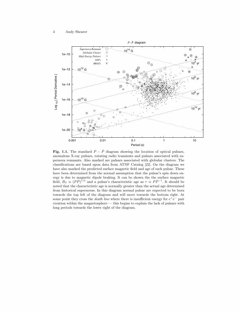
Figure 1.1 shows the P − P diagram for pulsars which gives a gross viewof a pulsar’s evolutionary position — normal pulsars are born towards the topof the diagram and move roughly towards the bottom right — i.e., they slowdown and it is this spin-down energy which powers the pulsar. The opticallyand higher photon energy emitting pulsars can be seen to be younger andtend to have higher magnetic fields and higher E values. Millisecond pulsars,which have been spun up through accretion are found in the bottom left ofdiagram illustrating their relatively weak magnetic fields. The binary natureof their progenitors also increases the chance that they are found in globularclusters.

4 Andy Shearer

"e!$%

"e!"&

"e!"'

"e!"(

"e!"$

"e!"%

%)%%" %)%" %)" " "%

*og

"% -

Perio

1 2

eriv

ativ

e 6

Perio1 7s9

!!! 1iagram

"%"( G

"%"% G

"%& G

"%"$ G

"%"% yr

"%& yr

"%' yr

"%( yr

"#$%&'()*+,%-'*'./0(1#0*&+20#3.%&

4567+8'%&69+!#03*&3:;!3,,:<3

Fig. 1.1. The standard P − P diagram showing the location of optical pulsars,anomalous X-ray pulsars, rotating radio transients and pulsars associated with su-pernova remnants. Also marked are pulsars associated with globular clusters. Theclassifications are based upon data from ATNF Catalog [22]. On the diagram wehave also marked the predicted surface magnetic field and age of each pulsar. Thesehave been determined from the normal assumption that the pulsar’s spin down en-ergy is due to magnetic dipole braking. It can be shown the the surface magneticfield, BS ∝ (PP )1/2 and a pulsar’s characteristic age as τ ≡ PP−1. It should benoted that the characteristic age is normally greater than the actual age determinedfrom historical supernovae. In this diagram normal pulsar are expected to be borntowards the top left of the diagram and will move towards the bottom right. Atsome point they cross the death line where there is insufficient energy for e+e− paircreation within the magnetosphere — this begins to explain the lack of pulsars withlong periods towards the lower right of the diagram.

1 High Time Resolution Astrophysics and Pulsars 5

Recently two new members of the neutron star zoo have been identified— AXPs, now thought to be magnetars and RRATs. The former are char-acterised by extremely high magnetic fields (> 1014 G) and are probablypowered by the decay of these fields. RRATs are the most recent neutron starobservation and are characterised by their transient radio signal, which oc-curs for a few milliseconds, at random intervals ranging from a few to severalhundred minutes. These different classes of pulsar are described below.

Since the first optical observations of the Crab pulsar in the late 1960s[6] only four more pulsars have been seen to pulsate optically (Vela [7]; PSRB0540−69 [8]; PSR B0656+14 [9]; PSR B0633+17 [10]). Four of these fivepulsars are probably too distant to have any detectable optical thermal emis-sion using currently available technologies. For the nearest and faintest pulsar,PSR B0633+17, spectroscopic studies have shown the emission to be predom-inantly non-thermal [11] with a flat featureless spectrum. For these objectswe are seeing non-thermal emission, presumably from interactions betweenthe pulsar’s magnetic field and a stream of charged particles from the neutronstar’s surface. Four other pulsars have been observed to emit optical radiation,but so far without any detected pulsations [12]. Optical pulsars seem to beless efficient than their higher energy counterparts with an average efficiency1

of about 10−9 compared to ≈ 10−2 at γ-ray energies [13]. Optical efficiencyalso decreases with age in contrast to γ-ray emission [14]. These factors com-bined indicate that pulsars are exceptionally dim optically, although it is inthe optical where it is potentially easier to extract important parameters fromthe radiation — namely spectral distribution, flux and polarisation.

Detailed time-resolved spectral observations have only been made of theCrab pulsar, but through broad-band photometry the spectral index of theother pulsars has been determined. Table 1.2 shows the spectral index for pul-sars with observed optical emission. If the emission mechanism is synchrotronand from a single location, you would expect the spectral index to be positivefor high frequencies changing to a value of 5/2 below the critical frequencyin the optically thick region where synchrotron self-absorption becomes dom-inant. One pulsar, PSR J0537−6910, which has not been observed opticallydespite showing many of the characteristics of the Crab pulsar, might be ex-pected to be more luminous. It is likely that synchrotron-self absorption willplay a significant part in reducing its optical flux [2], [15].

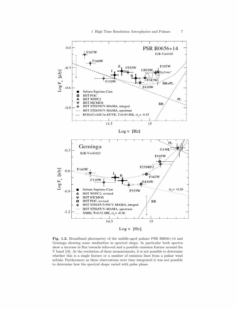
The other, optically fainter, pulsars have either had spectra taken with lowsignal-noise [11] or using broad band photometry had their gross spectral fea-tures determined. There have been suggestions of broadband features in thespectrum possibly associated with cyclotron absorption or emission features;Figure 1.2 shows the IR-NUV spectrum for PSR B0656+14 and Geminga [16].Until spectra with reasonable resolution have been taken we can not, with anydegree of certainty, characterise the spectra in term of absorption or emission

1 The optical efficiency is defined as the optical luminosity divided by the spindownenergy — (η ≡ Lν/E)

6 Andy Shearer

features. If a cyclotron origin for these features can be determined then wehave the possibility of determining the local magnetic field strength indepen-dently of the characteristic surface magnetic field (∝ (PP )−0.5). The over-all spectral shape is consistent with the UV dominated by thermal radiationfrom the surface and the optical-infrared region dominated by magnetosphericnon-thermal emission. Neither spectra show any evidence of synchrotron selfabsorption towards longer wavelengths.

Table 1.2. Optical Pulsars — Basic Data. Pulsars names marked in bold have beenobserved to pulsate. the spectral index covers the region from 3500–7000 A and isof the form Fν ∝ να. The spectral index are for time-averaged fluxes. The M31pulsar flux is based upon extrapolating the Crab pulsar to the distance of M31 andincreasing the noise background proportionately.

Pulsar mB Period Spectral VLT ELT(ms) Index B photons/rotation

Crab 16.8 33 -0.11 3,300 120,000PSR B0540−69 23 50 1.6 17 610Vela 24 89 0.12 12 440PSR B0656+14 25.5 385 0.45 13 470Geminga 26 237 1.9 25.5 200M31 (Crab) 30-31 33 - 0.02 1PSR B0950+08 27.1(V) 253 - - -PSR B1929+10 25.6(V) 227 - - -PSR B1055−52 24.9(V) 197 − - -PSR B1509−58 25.7(V) 151 - - -

Only one pulsar, the Crab, has had detailed polarisation measurementsmade [17], [18]. The polarisation profile shows emission aligned with the twomain peaks and is consistent with synchrotron emission. One unusual featureis the location of maximum polarisation which for the Crab pulsar precedesthe main pulse at a phase when the optical emission is at a minimum. Thepolarisation of one other, PSR B0656+14 [19] has been observed albeit atlow significance. This pulsar has maximum polarisation coincident with themaximum luminosity. Three other pulsars have only had their time averagepolarisation measured in the optical regime [20].

1.2.2 Emission Theory

Many suggestions have been made concerning the optical emission process forthese young and middle-aged pulsars. Despite many years of detailed theoret-ical studies and more recently limited numerical simulations, no convincingmodels have been derived which explain all of the high energy properties.There are similar problems in the radio, but as the emission mechanism isradically different (being coherent) only the high energy emission is consid-ered here. In essence despite nearly forty years of observations, we still do

1 High Time Resolution Astrophysics and Pulsars 7

Fig. 1.2. Broadband photometry of the middle-aged pulsars PSR B0656+14 andGeminga showing some similarities in spectral shape. In particular both spectrashow a increase in flux towards infra-red and a possible emission feature around theV band [16]. At the resolution of these measurements, it is not possible to determinewhether this is a single feature or a number of emission lines from a pulsar windnebula. Furthermore as these observations were time integrated it was not possibleto determine how the spectral shape varied with pulse phase.

8 Andy Shearer

not understand the emission mechanisms behind pulsar emission. The variouscompeting theories have all failed to provide a comprehensive description ofpulsar emission. Probably the only point of agreement between all these theo-ries is the association of pulsars with magnetized, rotating neutron stars [21].In the high energy regime there is more consensus as to the emission mech-anism — either incoherent synchrotron or curvature radiation for outer gapmodels or inverse Compton scattering for polar gap models. However, like ra-dio emission there is not a consensus as to the location of the emission regionor the acceleration mechanisms for the plasma.

1.2.3 Crab Pulsar

The Crab pulsar has been observed for nearly forty years. The earliest pho-tometric observations [25], [26] gave a visual magnitude of mV 16.5 ± 0.1compared to more recent observations [27] of mV 16.74 ± 0.05 in the sameperiod the pulsar has slowed by ≈1.5%. If we assume a L ∝ P−10 scalling lawthen in the same period the luminosity should have reduced by about 0.15magnitudes — in reasonable agreement with the observed luminosity decrease.

As can be seen from Table 1.2 the Crab Pulsar is uniquely bright amongstthe small population of optical pulsars. It is reasonably close (≈ 2 kpc) andless than one thousand years old. It is the only pulsar which is bright enoughfor individual pulses to be observed with any significant flux - allowing forpulse-pulse spectral and polarimetric changes to be observed. As a pulsar ithas unusual characteristics — for example it glitches and the radio emission isdominated by giant radio pulses (GRPs). The latter occur sporadically with amean repetition rate of about 1 Hz — the highest of the GRP emitting pulsars— see below. The Crab pulsar is seen to emit at all energies — from radio tohigh-energy γ-rays with E > 1 TeV. In the optical (UBV) regime the emissionis characterised by a flat power law Fν ∝ ν−0.07±0.18[23]. Although no directevidence of a roll-over in the spectrum has been observed there are hints thatin the near infra-red that the slope steepens ([15] and references therein).Recent Spitzer observations [24] possibly show the beginning of a rollover at≈2 µm. More detailed observations, particularly time-resolved from 1–50 µmwill be required to confirm this.

The Crab pulsar’s light curve, Figure 1.3, shows four distinct regions

• Main pulse containing about 50 % of the optical emission, the pulse has aFWHM of 4.5 % of the pulsar’s period

• Interpulse with about 30 % of the emission• Bridge with about 20 % of the emission• Off-pulse just before the main pulse where the polarisation percentage is

at a maximum

Spectral observations, of the Crab pulsar — both pulsed and time-integrated — have been made by a number of groups. All authors reportspectra that is generally flat and featureless — consistent with a synchrotron

1 High Time Resolution Astrophysics and Pulsars 9

(o)

(r)

(gr)

! " #

Bridge

InterpulsepulseMain optical

Flux

(arb

itrar

y un

its)

Phase of precursor

Phase (0,1 = radio phase)

0.2

0.4

0.6

0.8

1

1.2

0 0.5 1 1.5 2

0.4

0.6

0.8

1

0.98 1 1.02

Fig. 1.3. Crab pulsar’s light curve showing the main emission regions and therelationship between the optical light curve and its radio counterpart [30]. Theoptical data was taken using an APD based photometer on the William HerschelTelescope (WHT) each photon’s arrival time has been folded in phase with the pulsarradio ephemeris to produce the time averaged light curve. The radio data has beentreated in a similar fashion. Also shown is the location of a single giant radio pulse.

origin for the radiation with an integrated spectral index of 0.11. A possiblecyclotron absorption feature has been reported [27] although not seen by otherobservers. Of note are time resolved observations which indicate a change inthe spectral index on the leading and falling edge of the main and secondarypeaks [18], [28], [29]. As yet there is no clear explanation for either spectralshape changes, pulse width variations or polarimetry.

1.2.4 Giant Radio Pulse Pulsars — optical considerations

Six pulsars, see Table 1.3, exhibit giant radio pulse phenomena. Here, as wellas the normal radio emission, we see enhanced radio emission up to severaltimes the average occurring for a few percent of the total number of pulses.The Crab pulsar was itself discovered through its giant pulse phenomena [31].Phenomenologically these pulsars are a very diverse group with the only pos-sible common factor being their magnetic field strength at the light cylinder— the pulsars in Table 1.3 are all in the top six ranked by magnetic fieldstrength at the light cylinder. The sixth pulsar in the list of pulsars with highmagnetic field strength at the light cylinder, PSR J0537−6919 has only been

10 Andy Shearer

observed at X-ray energies and hence no giant radio emission. Two of thepulsars, the Crab and PSR J0540−6919, have very similar properties - young[age < 1000 years] pulsars embedded in a plerion. The other three are allmillisecond pulsars.

Observations of GRP pulsars at other energies has been difficult - primarilydue to the low rate of GRP events (ranging from 10−6 − 2 Hz) . γ-ray obser-vations [32] showed an upper limit of 2.5 times the average γ-ray flux basedupon 20 hours of simultaneous radio-γ-ray observations with CRGO/OSSEand the Greenbank 43m telescope. Optical observations [30] indicated a small(≈3%) increase in the optical flux during the same spin cycle as a GRP. Al-though the percentage increase was small the energy increase in the opticalpulse is comparable to the energy in the GRP. These results linked for thefirst time flux changes in the radio — where the emission is highly variable —to higher energy emission which is seen to be stable. Furthermore, given thedifferent emission mechanisms [coherent versus incoherent] such a correlationwas unexpected. Although small, the energy in the optical and radio GRPsare similar; if this were extrapolated to γ-ray energies we would expect anenhancement of <0.01%.

In two of these, PSR J1824−2452 and PSR J1939+2134, the GRP emis-sion aligns in phase with the X-ray pulse rather than the normal radio pulse[33][34]. This possibly implies a different emission zone and/or mechanism.Furthermore the spectrum of GRP fluxes shows a different slope to the nor-mal emission and cannot be regarded simply as its high flux extension. Whatcharacterises a GRP event compared to the high-energy tail of the normaldistribution is very subjective. An acceptable definition of what is and whatis not a GRP is that the pulses show a power-law energy distribution (cf. log-normal for typical pulsar emission) and have very short time-scales (typically≈ of nanosecond duration) [33]. Most studies have used a 10 or 20 〈E〉 criteriafor GRPs.

From an optical observational perspective GRPs are significantly more dif-ficult than normal pulsars to observe — the pulses arrive randomly albeit inphase with normal emission and at a rate significantly less than the normalpulsar rate. The random nature of GRP arrival times make synchronised sys-tems, such as clocked CCDs, inappropriate. Polarisation studies of these typeof event also restrict the type of polarimeter which can be used in the GRPstudies, and makes the simultaneous measurements of all Stokes’ parametersessential.

1.3 AXPs and RRATs

1.3.1 Anomalous X-Ray Pulsars

Anomalous X-Ray pulsars are a special class of neutron star characterised byvery high inferred magnetic fields and variable X-ray emission. Soft Gamma-ray repeaters (SGRs), first observed as transient γ-ray sources and now known

1 High Time Resolution Astrophysics and Pulsars 11

Table 1.3. Giant radio pulsars

Name Period Surface Field Light Cylinder GRP Ref.(ms) (109 G) Field (106G) Rate (Hz)

Crab 33.1 3800 9.8 1-2PSR J0540−6919 50.4 5000 3.7 0.001 [44]PSR J1824−2452 3.1 2.2 0.7 0.0003 [45]PSR J1959+2048 1.6 0.2 1.1PSR J1939+2134 1.6 0.4 1.0 0.0001 [46]PSR J0218+4231 0.03

1e!20

1e!18

1e!16

1e!14

1e!12

1e!10

0.001 0.01 0.1 1 10

Log

10 [

Perio

d D

eriv

ativ

e ]

Period (s)

P!P diagram

1010 G

108 G

1012 G

1014 G

1010 yr

108 yr

106 yr

104 yr104 G105 G106 G

GRP pulsarsLarge Amplitude Pulses

!BsurBlc

Fig. 1.4. The location of giant pulse emitters on the P − P diagram. We have alsoshown the inferred maximum magnetic field at the light cylinder based upon a 10km radius neutron star.

to be persistent sources of pulsed X-rays, show similar properties. Both AXPsand SGRs are thought to have similar physical properties and are likely to bemagnetars - where the emission comes from the decay of the strong magneticfield rather than being rotation powered. The review by Woods and Thompson[35] is a recent review of general AXP and SGR properties.

In Figure 1.1 AXPs are shown to be towards the top right of the P − Pdiagram. Models for their emission mechanism historically concentrated uponthe interaction between the neutron star and an accretion disk. However thelack of a secondary star precluded all but a fossil disk around the star. The

12 Andy Shearer

latter explanation was precluded by infrared observations [36]. The faintnessof the infrared counterpart precluded a disk model and strengthened the casefor the magnetar model where the high-energy emission comes from the decayof the strong magnetic field or from other magnetospheric phenomena.

Optical pulsed AXP emission was first observed from 4U 0142+61, us-ing a phase-clocked CCD [37] and confirmed by UltraCam observations [38].From Table 1.4 it can be seen that this pulsar is significantly brighter thanother AXPs in the infra-red and all suffer from significant reddening. All ofwhich combines to make future AXP optical observations very difficult anddependent on system such as Ultracam, but with better infra-red sensitivity.

Table 1.4. Optical and Infra-red properties AXPs and SGRs

Source P P B Magnitude(s) 10−11ss−1 1014 G V I J

SGR 0526−66 8.0 6.6 7.4 > 27.1 >25 -SGR 1627−41 6.4 >21.5SGR 1806−20 7.5 8.3-47 7.8 >21SGR 1900+14 5.2 6.1-20 5.7 > 22.84U 0142+61 8.69 0.196 1.3 25.6 23.8 -1E 10485937 6.45 3.9 3.9 26.2 21.7RXS 17084009 11.00 1.86 4.7 - - 20.91E 1841045 11.77 4.16 7.1 > 23(R) - -1E 2259+586 6.98 0.0483 0.60 >26.4(R) >25.6 >23.8AX J1845.00258 6.97 - - - -CXOU J0110043.1 8.02 - - - -XTE J1810197 5.54 1.15 2.9 - >24.3

1.3.2 Rotating Radio Transients

Rotating Radio Transients (RRATs) are a new class of pulsar that exhibitsporadic radio emission lasting for few milliseconds (2-30ms) at random in-tervals ranging from a few hundred seconds to several hours. Table 1.5, basedupon [39] details the basic RRAT parameters. For a few RRATs a periodicityand period derivative has been established by using the largest common divi-sor to estimate the period and in three cases the period derivative. It is notknown where these lie in the now expanding pulsar menagerie, however oneRRAT lies towards the magnetar region of the P − P diagram - see Figure1.1.

Todate no RRAT has had any optical counterpart observed, however Ul-traCam observations of PSRJ1819−1458 [40] produced an upper limit of 3.3,0.4 and 0.8 mJy at 3560, 4820 and 7610 A, respectively in 1800 seconds onthe WHT. The characteristics of the emission is difficult to determine at thisstage although the bursts do not seem to have the same form as Giant Radio

1 High Time Resolution Astrophysics and Pulsars 13

Pulses, for example they do not show a power law size distribution . One sug-gestion is that we are seeing a selection effect ([41]) — PSR B0656+14 wouldappear as an RRAT if it was located at a distance of greater than 3kpc. Thespread of derived periods is from 0.4-8 seconds which when combined withthe inferred surface magnetic field for one object being as high as 5 1013G wehave a possible link to AXPs and magnetars.

Table 1.5. Observational Properties of Rotating Radio Transients

Name Period P Distance Rate On(s) 10−15ss−1 (kpc) (hr−1) Time (10−5)

J0848−43 5.97748 - 5.5 1.4 1.2J1317−5759 2.6421979742 12.6 3.2 4.5 1.3J1443−60 4.758565 - 5.5 0.8 0.4J1754−30 0.422617 2.2 0.6 0.3J1819−1458 4.263159894 50.16 3.6 17.6 1.5J1826−14 0.7706187 3.3 1.1 0.06J1839−01 0.93190 6.5 0.6 0.3J1846−02 4.476739 5.2 1.1 0.5J1848−12 6.7953 2.4 1.3 0.07J1911+00 - 3.3 0.3 0.04J1913+1333 0.9233885242 7.87 5.7 4.7 0.3

1.4 Future Observing Campaigns

Despite forty years of of observation there are still a number of fundamentalunanswered question in pulsar astrophysics. In the optical regime we can bebegin to answer these question if we have a larger and more comprehensivesurvey of normal pulsars. Most pulsed observations were made on mediumsized (4-6 m) telescopes using detectors with modest or low quantum efficien-cies. By moving to larger 8-10 m class telescopes we gain about a magnitudein our upper limits. By using more efficient detectors another two magnitudeimprovement is possible making pulsed observations of 27th magnitude ob-jects plausible in one night. Figure 4 shows a measure of the observability(ranked according to flux) (E/d2) of known pulsars. If we take, an admittedlyarbitrary, level of 1035 ergs sec−1 kpc−2 we have 20-30 pulsars which couldbe observed using current technology. From Figure 1.5 there is a rough dividearound pulsar periods around 50-100 ms below which non-CCD technolo-gies (Superconducting Tunnel Junction (STJ) devices [42], Transition EdgeSensors (TES) [43], APDs) are appropriate. In all cases polarisation measure-ments will be important as they give information of the local magnetic fieldstrength and geometry. Spectral information, to look for synchrotron self ab-sorption and cyclotron features, will give important clues to the strength of

14 Andy Shearer

1028

1030

1032

1034

1036

1038

0.001 0.01 0.1 1 10

! "#$#% (e

rgs

s!1 k

pc!2

)

Period (s)

P!! "$#% diagram

Pulsed Optical EmissionNon!pulsed Optical Emission

High Energy Emission

Fig. 1.5. Observability diagram

the magnetic field in the emission zone and thus its height above the neutronstar surface. In the future coordinated campaigns, particularly simultaneousradio-optical observations, can be used to look for specific phenomena suchas GRPs and RRATs.

Normal PulsarsOnly five normal pulsars have had observed pulsed optical emission. From

such a small sample it is not possible, particularly with the lack of an ac-ceptable theory for pulsar emission, to make any strong conclusions. Howeverwith high quantum efficiency detectors and larger telescopes we can reason-ably expect an increased sample of optical pulsars over the next 5-10 years.Specifically if we take the optical luminosity to scale with the spin down en-ergy ( LO ∝ E1.6) [14] then we can estimate the number of pulsars whichare potentially observable. This is a very approximate relationship designedto indicate which pulsars are more likely to observed with current telescopesand instrumentation. From Table 1.6 the following pulsars can be potentiallyobserved with 4-8m class telescopes with current optical detectors — PSRJ0205+6449, PSR J1709−4429, PSR J1513−5908, PSR J1952+3252, PSRJ1524−5625, PSR J0537−6910 and PSR J2229+6114.

1 High Time Resolution Astrophysics and Pulsars 15

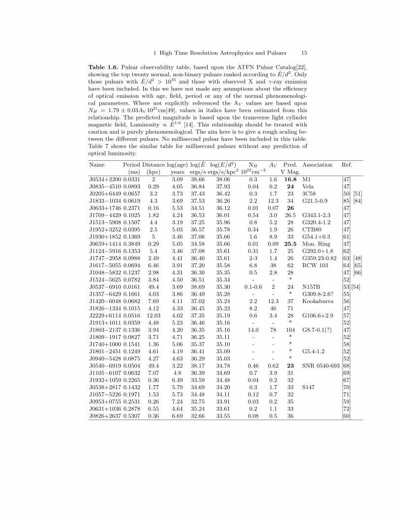
Table 1.6. Pulsar observability table, based upon the ATFN Pulsar Catalog[22],showing the top twenty normal, non-binary pulsars ranked according to E/d2. Onlythose pulsars with E/d2 > 1035 and those with observed X and γ-ray emissionhave been included. In this we have not made any asumptions about the efficiencyof optical emission with age, field, period or any of the normal phenomenologi-cal parameters. Where not explicitly referenced the AV values are based uponNH = 1.79 ± 0.03AV 1021cm[49], values in italics have been estimated from thisrelationship. The predicted magnitude is based upon the transverse light cylindermagnetic field, Luminosity ∝ E1.6 [14]. This relationship should be treated withcaution and is purely phenomenological. The aim here is to give a rough scaling be-tween the different pulsars. No millisecond pulsar have been included in this table.Table 7 shows the similar table for millisecond pulsars without any prediction ofoptical luminosity.

Name Period Distance log(age) log(E log( ˙E/d2) NH AV Pred. Association Ref.(ms) (kpc) years ergs/s ergs/s/kpc2 1022cm−2 V Mag.

J0534+2200 0.0331 2 3.09 38.66 38.06 0.3 1.6 16.8 M1 [47]J0835−4510 0.0893 0.29 4.05 36.84 37.93 0.04 0.2 24 Vela [47]J0205+6449 0.0657 3.2 3.73 37.43 36.42 0.3 1.7 23 3C58 [50] [51]J1833−1034 0.0619 4.3 3.69 37.53 36.26 2.2 12.3 34 G21.5-0.9 [85] [84]J0633+1746 0.2371 0.16 5.53 34.51 36.12 0.01 0.07 26 [47]J1709−4429 0.1025 1.82 4.24 36.53 36.01 0.54 3.0 26.5 G343.1-2.3 [47]J1513−5908 0.1507 4.4 3.19 37.25 35.96 0.8 5.2 28 G320.4-1.2 [47]J1952+3252 0.0395 2.5 5.03 36.57 35.78 0.34 1.9 26 CTB80 [47]J1930+1852 0.1369 5 3.46 37.06 35.66 1.6 8.9 33 G54.1+0.3 [61]J0659+1414 0.3849 0.29 5.05 34.58 35.66 0.01 0.09 25.5 Mon. Ring [47]J1124−5916 0.1353 5.4 3.46 37.08 35.61 0.31 1.7 25 G292.0+1.8 [62]J1747−2958 0.0988 2.49 4.41 36.40 35.61 2-3 1.4 26 G359.23-0.82 [63] [48]J1617−5055 0.0694 6.46 3.91 37.20 35.58 6.8 38 62 RCW 103 [64] [65]J1048−5832 0.1237 2.98 4.31 36.30 35.35 0.5 2.8 28 [47] [66]J1524−5625 0.0782 3.84 4.50 36.51 35.34 - - * [52]J0537−6910 0.0161 49.4 3.69 38.69 35.30 0.1-0.6 2 24 N157B [53][54]J1357−6429 0.1661 4.03 3.86 36.49 35.28 - - * G309.8-2.6? [55]J1420−6048 0.0682 7.69 4.11 37.02 35.24 2.2 12.3 37 Kookaburra [56]J1826−1334 0.1015 4.12 4.33 36.45 35.22 8.2 46 71 [47]J2229+6114 0.0516 12.03 4.02 37.35 35.19 0.6 3.4 28 G106.6+2.9 [57]J1913+1011 0.0359 4.48 5.23 36.46 35.16 - - * [52]J1803−2137 0.1336 3.94 4.20 36.35 35.16 14.0 78 104 G8.7-0.1(?) [47]J1809−1917 0.0827 3.71 4.71 36.25 35.11 - - * [52]J1740+1000 0.1541 1.36 5.06 35.37 35.10 - - * [58]J1801−2451 0.1249 4.61 4.19 36.41 35.09 - - * G5.4-1.2 [52]J0940−5428 0.0875 4.27 4.63 36.29 35.03 - - * [52]J0540−6919 0.0504 49.4 3.22 38.17 34.78 0.46 0.62 23 SNR 0540-693 [68]J1105−6107 0.0632 7.07 4.8 36.39 34.69 0.7 3.9 31 [69]J1932+1059 0.2265 0.36 6.49 33.59 34.48 0.04 0.2 32 [67]J0538+2817 0.1432 1.77 5.79 34.69 34.20 0.3 1.7 33 S147 [70]J1057−5226 0.1971 1.53 5.73 34.48 34.11 0.12 0.7 32 [71]J0953+0755 0.2531 0.26 7.24 32.75 33.91 0.03 0.2 35 [59]J0631+1036 0.2878 6.55 4.64 35.24 33.61 0.2 1.1 33 [72]J0826+2637 0.5307 0.36 6.69 32.66 33.55 0.08 0.5 36 [60]

16 Andy Shearer

Table 1.7. Millisecond pulsar observability table, based upon the ATFN PulsarCatalog [22]

Name Period Distance log(age) log(E log( ˙E/d2) Ref.(ms) (kpc) years ergs/s ergs/s/kpc2

J2124−3358 4.93 0.25 9.6 33.8 35.0 [73]J1824−2452 3.05 4.9 7.5 36.4 35.0 [47]J1939+2134 1.56 3.6 8.4 36.0 34.9 [47]J0030+0451 4.87 0.23 9.9 33.5 34.8 [73]J1024−0719 5.16 0.35 9.6 33.7 34.6 [74]J1744−1134 4.08 0.36 9.9 33.7 34.6 [74]J1843−1113 1.85 1.97 9.5 34.8 34.2 [75]J1823−3021A 5.44 7.9 7.4 35.9 34.1 [47]J0024−7204F 2.62 4.8 8.8 35.1 33.8 [76]J1730−2304 8.12 0.51 9.8 33.2 33.8 [77]J2322+2057 4.81 0.78 9.9 33.5 33.8 [47]J0711−6830 5.49 1.04 9.8 33.6 33.5 [78]J1910−5959D 9.04 4 8.2 34.7 33.5 [79]J1944+0907 5.19 1.28 9.7 33.7 33.5 [80]J1721−2457 3.50 1.56 10.0 33.7 33.4 [81]J1905+0400 3.78 1.34 10.1 33.5 33.3 [75]J1801−1417 3.63 1.8 10.0 33.6 33.1 [82]

Optical GRP observations are currently limited to the Crab pulsar andlikely to remain so for the foreseeable future. The frequency of GRP eventsis very low with all other GRP emitters and only one of which (PSRJ0540−6919) has been observed optically. If PSR J0540−6919 behaves in asimilar manner to the Crab pulsar then the observed GRP rate of 0.001 Hz,about 1000 times lower than the Crab, will have a corresponding increasein observing time making optical observations unlikely in the near future. IfPSR J0540−6919 shows a 3% increase in optical flux during GRP events thendetecting this at the 3 σ level would require over 100 hours of observationusing the 8m VLT and an APD based detector.

Millisecond PulsarsWith the exception of UV observations of the PSR J0437−4715 [83] there

are no optical counterparts of any millisecond pulsar and in the case of PSRJ0437−4715 the optical emission is probably thermal in origin. There havebeen a few upper limits and possible, but unconfirmed, counterparts. Until anumber of optical millisecond pulsars has been observed, it will be difficultto even estimate the number of millisecond pulsars we can expect to observeoptically . Table 1.7 shows those millisecond pulsars with the highest E/d2,which which we regard as a starting point for selecting those pulsars suitablefor optical study.

AXPs

1 High Time Resolution Astrophysics and Pulsars 17

AXPs have typical periods in the range 8-12 seconds and consequentlycan be observed with conventional CCDs or Low-Light-Level CCDs (L3CCD).They also are characterised by high magnetic fields indicating that polarisa-tion will be an important component of any future instrument and programmeof observations. However the number of known AXPs is small and most haveupper limits which are significantly lower than the detected flux from 4U0142+61 making significant optical observations unlikely in the short term.In the near-IR recent observations of 4U 0142+61 [86] are consistent with theexistence of a cool (T ≈ 91 K) debris disk around the neutron star. We wouldexpect, if this is confirmed, that the pulse fraction in the near-IR should belower than in the optical wavebands. It is interesting to speculate whethersimilar features could be observed in young normal pulsars..

RRATsObserving RRATs in the optical will be a serious observational challenge

requiring coordinated optical/radio-observations. For example PSRJ1819−1458was observed for ≈ 1800 seconds with UltraCam which produced upper mag-nitude limits of 15.1, 17.4 and 16.6 in u′, g′ and i′. If only those framescoincident with radio events were recorded then this would have produced 3σlimits of 16.7, 18.8 and 18.1 respectively. If the link to AXPs is real then wemust obtain peak i′ magnitudes of about 24 or unrealistic exposure times of ≈71 hours using UltraCam. Even if we use a detector with zero read noise (e.g.L3CCDs or APDs) then our exposure times drop down to 57 hours, for a 3 σdetection. Alternatively if, as with GRPs, the energy in the radio and opticaltransient are similar then we would expect observation times of roughly 10hours with UltraCam to achieve a 3 σ detection. Another way of looking atthe RRAT detection probability is to scale according to the fractional on-timeof each RRAT. PSR J1819−1458 is radiating for approximately 0.01% of thetime or 10 magnitudes down from a pulsar which is radiating continuously. Incontrast PSR J1848−12 is a further factor of 100 weaker.

1.5 Conclusion

Optical/infra-red observations of pulsars of all types are still in their relativeinfancy with very few objects detected. The likelihood is that in the next 5years the number of pulsars with detected optical emission will have doubledand more significantly, new observations will include polarisation measure-ments. With respect to high energy emission, it is only at optical energieswhere it is possible to measure, with reasonable accuracy, all electro-magneticaspects of pulsar radiation. These later observations, combined with detailednumerical models should elucidate, through geometric arguments, the struc-ture of the emission zone for normal pulsars and hence provide stringent ob-servational tests for the various models of pulsar emission. In the future ELTs

18 Andy Shearer

with adaptive optics will enable pulsar observations down to 32-33 magnitudeand importantly will enable spectra-polarimetry down to 29-30 magnitude.

Beyond this time into the ELT era there is the possibility of extending thenumber of optically observed pulsars (and pulsar types) dramatically. Thiswill require detectors with :-

• High-time resolution — both frame based systems from 1 ms+ and pixelread-outs for τ < 1 ms

• Medium size arrays — wide-field operations are not required but nearbyreference stars are needed - array sizes > 32 × 32

• Polarisation — sensitive to polarisation changes - both circular and linearat the 1% level

• Energy Resolution — Broad-medium band energy resolution - 1-10%

References

1. Hankins, T. H., Kern, J. S., Weatherall, J. C., & Eilek, J. A., 2003, Nature,422, 141

2. Pacini, F., 1971, ApJ, 163, L173. Baade, W. & Zwicky, F., 1934, Proc. Nat. Acad. Sci, 20:5, 2594. Pacini, F, 1967, Nature, 216, 5675. Hewish, A., Bell, S. J., Pilkington, J. D., Scott, P. F. & Collins, R. A., 1968,

Nature, 217, 7096. Cocke, W. J., Disney, M. J. & Taylor, D. J., 1969, Nature, 221, 5257. Wallace, P. T. et al., 1977, Nature, 266, 6928. Middleditch, J. & Pennypacker, C., 1985, Nature, 313, 6599. Shearer, A., Redfern, R. M., Gorman, G., Butler, Golden, A., R., O’Kane, P.,

Golden, A., Beskin, G. M., Neizvestny, S. I., Neustroev, V. V., Plokhotnichenko,V. L. & Cullum, M., 1997, ApJ, 487, L181

10. Shearer, A., Harfst, S., Redfern, R. M., Butler, R., O’Kane, P., Beskin, G. M.,Neizvestny, S. I., Neustroev, V. V., Plokhotnichenko, V. L. & Cullum, M., 1998,A & A, 335, L21

11. Martin, C, Halpern, J.P. & Schiminovich, D., 1998, ApJ, 494, L21112. Mignani, R. P., 2005, astro-ph/050216013. Lorimer, D. & Kramer, M., 2005, Handbook of Pulsar Astronomy, Cambridge

University Press, ISBN 0 521 82823 614. Shearer, A & Golden, G, 2001, ApJ, 547, 96715. O Connor, P Golden, A & Shearer, A, 2005, ApJ, 631, 47116. Shibanov, Y. A, Zharikov, S. V., Komarova, V. N., Kawai, N. , Urata, Y., A. B.

Koptsevich, A. B., Sokolov, V. V., Shibata, S. & N. Shibazaki, N, 2006, A&A,448, 313

17. Smith, F. G., Jones, D. H. P., Dick, J. S. B. & Pike, C. D., 1988, MNRAS, 233,305

18. Romani, R. W., Miller, A. J., Cabrera, B., Nam, S. W. & Martinis, J. M., 2001,ApJ, 563, 221

19. Kern, B., Martin, C., Mazin, B. & Halpern, J. P., 2003, ApJ, 597, 104920. Wagner, Stefan J. & Seifert, W., 2000, ASPC, 202, 315

1 High Time Resolution Astrophysics and Pulsars 19

21. Lyutikov, M., Blandford, R., & Machabeli, G., 1999, MNRAS, 305, 33822. Manchester, R. N., Hobbs, G. B., Teoh, A. & Hobbs, M., 2005, AJ, 129, 199323. Golden, A., Shearer, A., Redfern, R. M., Beskin, G. M., Neizvestny, S. I.,

Neustroev, V. V., Plokhotnichenko, V. L. & Cullum, M., 2000, A&A, 363,617

24. Temim, T., Gehrz, R. D., Woodward, C. E., Roellig, T. L., Smith, N., Rudnick,L., Polomski, E. F., Davidson, K., Yuen, L. & Onaka, T., 2006, AJ, 132, 1610

25. Neugebauer, G., Becklin, E. E., Kristian, J., Leighton, R. B., Snellen, G. &Westphal, J. A., 1969, ApJ, 156, 133

26. Kristian, J., Visvanathan, N., Westphal, J. A. & Snellen, G. H., 1970, ApJ,162, 475

27. Nasuti, F. P., Mignani, R., Caraveo, P. A. & Bignami, G. F., 1996, A&A, 314,849

28. Fordham, J. L. A., Vranesevic, N., Carraminana, A., Michel, R., Much, R.,Wehinger, P. & Wyckoff, S., 2002, ApJ, 581, 485

29. Eikenberry, S. S., Fazio, G. G., Ransom, S. M., Middleditch, J., Kristian, J., &Pennypacker, C. R. 1997, ApJ, 477, 465

30. Shearer, A., Stappers, B., O’Connor, P., Golden, A., Strom, R., Redfern, M.,and Ryan, O. , 2003, Science, 301, 493

31. Staelin, D. H. & Reifenstein, E. C. III, 1968, Science, 162, 148132. Lundgren, S. C., Cordes, J. M., Ulmer, M., Matz, S. M., Lomatch, S., Foster,

R. S. & Hankins, T., 1995, ApJ, 453, 43333. Romani, R., & Johnston, S., 2001, ApJ, 557, L9334. Cusumano, G., Hermsen, W., Kramer, M., Kuiper, L., Lhmer, O., Massaro, E.,

Mineo, T., Nicastro, L., & Stappers, B. W., 2003, A&A, 410, L935. Woods, P. & Thompson, C, 2004, astro-ph/040613336. Hulleman, F., van Kerkwijk, M. H. & Kulkarni, S. R., 2000, Nature, 408, 68937. Kern, B. & Martin, C., 2002, Nature, 417, 52738. Dhillon, V. S., Marsh, T. R., Hulleman, F., van Kerkwijk, M. H., Shearer, A.,

Littlefair, S. P., Gavriil, F. P. & Kaspi, V. M., 2005, MNRAS, 363, 60939. McLaughlin M. A., Lyne A. G., Lorimer D. R., Kramer M., Faulkner A. J.,

Manchester R. N., Cordes J. M., Camilo F., Possenti A., Stairs I. H., HobbsG., DAmico N., Burgay M., OBrien J. T., 2006, Nature, 439, 817

40. Dhillon, V. S., Marsh, T. R.& Littlefair, S. P. 2006, MNRAS, 372, 20941. Weltevrede, P., Stappers, B. W., Rankin, J. M. & Wright, G. A. E., 2006, ApJ,

645, L14942. Perryman, M. A. C., Favata, F., Peacock, A., Rando, N. & Taylor, B. G., 1999,

A&A, 346, L3043. Romani, R. W., Burney, J., Brink, P., Cabrera, B., Castle, P., Kenny, T., Wang,

E., Young, B., Miller, A. J. & Nam, S. W., 2003, ASP Conference Proceedings,291, 399

44. Johnston, S & Romani, R. W., 2003, ApJ, 590, L9545. Johnston, S & Romani, R. W., 2003, ApJ, 557, L9346. Soglasnov, V. A., Popov, M. V., Bartel, N., Cannon, W., Novikov, A. Yu.,

Kondratiev, V. I. & Altunin, V. I., 2004, ApJ, 616, 43947. Becker, W. & Trumper, J., 1997, A&A, 326, 68248. Gaensler, B. M., van der Swaluw, E., Camilo, F., Kaspi, V. M., Baganoff, F.

K., Yusef-Zadeh, F. & Manchester, R. N., 2004, ApJ, 616, 38349. Predehl, P. & Schmitt, J. H. M. M., 1995, A & A, 293, 889

20 Andy Shearer

50. Helfand, D. J., Becker, R. H., & White, R. L. 1995, ApJ, 453, 74151. Torii, K., Slane, P. O., Kinigasa, K., Hashimotodani, K., & Tsunemi, H., 2000,

PASJ, 52, 87552. Kramer, M., et al., 2003, MNRAS, 342, 129953. Marshall, F. E., Gotthelf, E. V., Zhang, W., Middleditch, J. & Wang, Q. D,

1998, Apj, 499, 17954. Townsley, L. K., Broos, P. S., Feigelson, E. D., Brandl, B. R.; Chu, Y-H,

Garmire, G. P. & Pavlov, G. G., 2006, AJ, 131, 214055. Camilo, F. et al, 2004, ApJ, 611, L2556. Roberts, M. S. E., Romani, R. W. & Johnston, S., 2001, ApJ, 561, 18757. Halpern, J. P., Camilo, F., Gotthelf, E. V., Helfand, D. J., Kramer, M., Lyne,

A. G., Leighly, K. M. & Eracleous, M., 2001, ApJ, 552, L12558. McLaughlin, M. A., Arzoumanian, Z., Cordes, J. M., Backer, D. C., Lommen,

A. N., Lorimer, D. R. & Zepka, A. F., 2002, ApJ, 564, 33359. Zavlin, V. & Pavlov, G., 2004, A&A, 616, 45260. Becker, W., Weisskopf, M. C., Tennant, Allyn F., Jessner, A., Dyks, J., Harding,

A. K., Zhang, S. N., 2004, ApJ, 615, 90861. Lu, F. J., Wang, Q. D., Aschenbach, B., Durouchoux, P. & Song, L. M., 2002,

ApJ, 568, L4962. Hughes, J. P., Slane, P. O., Park, S., Roming, P. W. A. & Burrows, D. N., 2003,

ApJ, 591, 13963. Camilo, F., Manchester, R. N, Gaensler, B. M. & Lorimer, D. R., 2002, ApJ,

579, L2564. Torii, K., Kinugasa, K., Toneri, T., Asanuma, T., Tsunemi, H., Dotani, T.,

Mitsuda, K., Gotthelf, E. V. & Petre, R., 1998, ApJ, 494, 20765. Gotthelf, E. V., Petre, R., & Hwang, U., 1997, ApJ, 487, L17566. Pivovaroff, M. J., Kaspi, V. M. & Gotthelf, E. V., 2000, ApJ, 528, 43667. Becker, W., Kramer, M., Jessner, A., Taam, R. E., Jia, J. J., Cheng, K. S.,

Mignani, R., Pellizzoni, A., de Luca, A., lowikowska, A. S. & Caraveo, P.A.,2006, ApJ, 645, 1421

68. Serafimovich, N. I., Shibanov, Yu. A.. Lundqvist, P. & Sollerman, J., 2004,A&A, 425 1041

69. Gotthelf, E. V. & Kaspi, V. M., 1998, ApJ, 497, L2970. Romani, R. W. & Ng, C.-Y., 2003, ApJ, 585, L4171. Mignani, R., Caraveo, P. A. & Bignami, G. F., 1997, ApJ, 474, L5172. Torii, K., Saito, Y., Nagase, F., Yamagami, T., Kamae, T., Hirayama, M.,

Kawai, N., Sakurai, I., Namiki, M., Shibata, S., Gunji, S. & Finley, J. P., 2000,ApJ, 551, L151

73. Becker, W., Trumper, J., Lommen, A. N. & Backer, D. C., 2000, ApJ, 561, 30874. Sutaria, F. K., Ray, A., Reisenegger, A., Hertling, G., Quintana, H. & Minniti,

D., 2003, A&A, 406, 24575. Hobbs, G., Faulkner, A., Stairs, I. H., Camilo, F., Manchester, R. N., Lyne, A.

G., Kramer, M., D’Amico, N., Kaspi, V. M., Possenti, A., McLaughlin, M. A.,Lorimer, D. R., Burgay, M., Joshi, B. C.& Crawford, F., 2004, MNRAS, 352,1439

76. Robinson, C. R., Lyne, A. G., Manchester, A. G., Bailes, M., D’Amico, N., &Johnston, S. 1995, MNRAS, 274, 547

77. Lorimer, D. R., Nicastro, L., Lyne, A. G., Bailes, M., Manchester, R. N., John-ston, S., Bell, J. F., D’Amico, N. & Harrison, P. A., 1995, ApJ, 439, 933

1 High Time Resolution Astrophysics and Pulsars 21

78. Bailes, M., Johnston, S., Bell, J. F., Lorimer, D. R., Stappers, B. W., Manch-ester, R. N., Lyne, A. G., Nicastro, L., D’Amico, N. & Gaensler, B. M., 1997,ApJ, 481, 386

79. D’Amico, N., Lyne, A. G., Manchester, R. N., Possenti, A., & Camilo, F. 2001,ApJ, 548, L171

80. Champion, D. J., Lorimer, D. R., McLaughlin, M. A., Xilouris, K. M., Arzou-manian, Z., Freire, P. C. C., Lommen, A. N., Cordes, J. M. & Camilo, F., 2005,MNRAS, 363, 929

81. Edwards, R. T. & Bailes, M., 2001, ApJ, 553, 80182. A. J. Faulkner, I. H. Stairs, M. Kramer, A. G. Lyne, G. Hobbs, A. Possenti, D.

R. Lorimer, R. N. Manchester, M. A. McLaughlin, N. D’Amico, F. Camilo &M. Burgay, 2004, MNRAS, 355, 147

83. Kargaltsev, O., Pavlov, G. & Romani, R. W., 2004, ApJ, 602, 37284. Camilo, F.,Ransom, S. M.,Gaensler, B. M., Slane, P. O., Lorimer, D. R.,

Reynolds, J., Manchester, R. N. & Murray, S. S, 2006, ApJ, 637, 45685. Safi-Harb, S., Harrus, I. M., Petre, R., Pavlov, G. G., Koptsevich, A. B. &

Sanwal, D. 2001,86. Wang, Z., Chakrabarty, D. & Kaplan, D. L., 2006, Nature, 440, 772