1 An Introduction to Event-Related Potentials and Their ...

1 An Introduction to Event-Related Potentials and Their Neural Origins

This chapter introduces the event-related potential (ERP) technique. The first section describes the goals of this book and discusses the perspective from which I've written it. The second section provides a brief history of the ERP technique. The third section describes two simple ERP experiments as examples that introduce some of the basic concepts of ERP experimentation. The fourth section describes the advantages and disadvantages of the ERP technique in relation to other techniques. The fifth section describes the neural and biophysical origins of ERPs and the associated event-related magnetic fields. The final section contains a brief description of the most commonly observed ERP components in cognitive neuroscience experiments.

Goals and Perspective This book is intended as a guidebook for people who wish to use ERPs to answer questions of broad interest in cognitive neuroscience and related fields. This includes cognitive scientists who plan to use ERPs to address questions that are essentially about cognition rather than questions that are essentially about neuroscience. The book should also be very useful for researchers in the growing area of affective neuroscience, as well as those in the area of psychopathology. It also provides a good background for researchers and students who encounter ERP studies in the literature and want to be able to understand and evaluate them.

The book was written for people who are just starting to do ERP research and for people who have been doing it for a few years and would like to understand more about why things are done in

3 Chapter 1 2

a parHcular way. ERP experts may find it useful as a reference (and they would probably learn something new by reading chapter 5, which provides a fairly detailed account of filtering that is approachable for people who don't happen to have an advanced degree in electrical engineering).

The book provides practical descriptions of straightforward methods for recording and analyzing ERPs, along with the theoretical background to explain why these are particularly good methods. The book also provides some advice about how to design ERP experiments so that they will be truly useful in answering broadly significant questions (i.e., questions that are important to people who don't themselves conduct ERP experiments). Because the goal of this book is to provide an introduction to ERPs for people who are not already experts, I have focused on the most basic techniques and neglected many of the more sophisticated approaches (although I have tried to at least mention the most important of them). For a broader treatment, aimed at experts, see David Regan's massive treatise (Regan, 1989).

To keep things simple, this book focuses primarily on the techniques used in my own laboratory (and in many of the world's leading ERP labs). In most cases, these are techniques that I learned as a graduate student in Steve Hillyard's laboratory at University of California, San Diego, and they reflect a long history of electrophysiological recordings dating back to Hallowell Davis's lab in the 1930s (Davis was the mentor of Bob Galambos, who was the mentor of Steve Hillyard; Galambos was actually a subject in the first sensory ERP experiments, described in the next section). Other approaches to ERP experimentation may be just as good or even better, but the techniques described here have stood the test of time and provide an excellent foundation for more advanced approaches.

This book reflects my own somewhat idiosyncratic perspective on the use of ERP recordings in cognitive neuroscience, and there are two aspects of this perspective that deserve some comment. First, although much of my own research uses ERP recordings, I

An Introduction to Event·Related Potentials and Their Neural Origins

believe that the ERP technique is well suited to answering only a small subset of the questions that are important to cognitive neuroscientists. The key, of course, is figuring out which issues this technique best addresses. Second, I take a relatively low-tech approach to ERPs. In the vast majority of cases, I believe that it is better to use a modest number of electrodes and fairly simple data analysis techniques instead of a large array of electrodes and complicated data analysis techniques. This is heresy to many ERP researchers, but the plain fact is that ERPs are not a functional neuroimaging technique and cannot be used to definitively localize brain activity (except under a very narrow set of conditions). I also believe that too much has been made of brain localization. with many researchers seeming to assume that knowing where a cognitive process happens is the same as knowing how it happens. In other words, there is much more to cognitive neuroscience than functional neuroanatomy, and ERPs can be very useful in elucidating cognitive mechanisms and their neural substrates even when we don't know where the ERPs are generated.

ABit of History In 1929, Hans Berger reported a remarkable and controversial set of experiments in which he showed that one could measure the electrical activity of the human brain by placing an electrode on the scalp. amplifying the signal, and plotting the changes in voltage over time (Berger, 1929). This electrical activity is called the electroencephalogram. or EEG. The neurophysiologists of the day were preoccupied with action potentials, and many of them initially believed that the relatively slow and rhythmic brain waves Berger observed were some sort of artifact. After a few years, however, the respected physiologist Adrian (Adrian & Matthews, 1934) also observed human EEG activity, and Jasper and Carmichael (1935) and Gibbs, Davis, and Lennox (1935) confirmed the details of Berger's observations. These findings led to the acceptance of the EEG as a real phenomenon.

5 Chapter 1 4

Over the ensuing decades, the EEG proved to be very useful in both scientific and clinical applications. In its raw form, however, the EEG is a very coarse measure of brain activity, and it is very difficult to use it to assess the highly specific neural processes that are the focus of cognitive neuroscience. The drawback of the EEG is that it represents a mixed up conglomeration of hundreds of different neural sources of activity, making it difficult to isolate individual neuro-cognitive processes. However, embedded within the EEG are the neural responses associated with specific sensory, cognitive. and motor events, and it is possible to extract these responses from the overall EEG by means of a simple averaging technique (and more sophisticated techniques, as well). These specific responses are called event-related potentials to denote the fact that they are electrical potentials associated with specific events.

As far as I can tell, the first unambiguous sensory ERP recordings from awake humans were performed in 1935-1936 by Pauline and Hallowell Davis, and published a few years later (Davis et a\.. 1939; Davis. 1939). This was long before computers were available for recording the EEG, but the researchers were able to see clear ERPs on single trials during periods in which the EEG was quiescent (the first published computer-averaged ERP waveform were apparently published by Galambos and Sheatz in 1962). Not much ERP work was done in the 1940s due to World War II, but research picked up again in the 1950s. Most of this research focused on sensory issues, but some of it addressed the effects of top-down factors on sensory responses.

The modern era of ERP research began in 1964, when Grey Walter and his colleagues reported the first cognitive ERP component, which they called the contingent negative variation or CNV (Walter et aI., 1964). On each trial of this study, subjects were presented with a warning signal (e.g., a click) followed 500 or 1,000 ms later by a target stimulus (e.g., a series of flashes). In the absence of a task, each of these two stimuli elicited the sort of sensory ERP response that one would expect for these stimuli. However, if sub-

An Introduction to Event-Related Potentials and Their Neural Origins

jects were required to press a button upon detecting the target, a large negative voltage was observed at frontal electrode sites during the period that separated the warning signal and the target. This negative voltage-the CNV-was clearly not just a sensory response. Instead, it appeared to reflect the subject's preparation for the upcoming target. This exciting new finding led many researchers to begin exploring cognitive ERP components.

The next major advance was the discovery of the P3 component by Sutton, Braren, Zubin, and John (1965). They found that when subjects could not predict whether the next stimulus would be auditory or visual, the stimulus elicited a large positive P3 component that peaked around 300 ms poststimulus; this component was much smaller when the modality of the stimulus was perfectly predictable. They described this result in terms of information theory, which was then a very hot topic in cognitive psychology. and their paper generated a huge amount of interest. To get a sense of the impact of this study, I ran a quick MedUne search and found about sixteen hundred journal articles that refer to the P300 (or P3) component in the title or abstract. This search probably missed at least half of the articles that talk about the P300 component. so this is an impressive amount of research. In addition, the Sutton et al. (1965) paper has been cited almost eight hundred times. There is no doubt that many millions of dollars have been spent on P300 studies (not to mention the many marks, pounds, yen, etc.).

Over the ensuing fifteen years, a great deal of research focused on identifying various cognitive ERP components and developing methods for recording and analyzing ERPs in cognitive experiments. Because people were so excited about being able to record human brain activity related to cognition, ERP papers in this period were regularly published in Science and Nature (much like the early days of PET and fMRI research). Most of this research was focused on discovering and understanding ERP components rather than using them to address questions of broad scientific interest. I like to call this sort of experimentation ERPology, because it is simply the study of ERPs.

7 Chapter 1 6

ERPology plays an important role in cognitive neuroscience, because it is necessary to know quite a bit about specific ERP components before one can use them to study issues of broader importance. Indeed, a great deal of ERPology continues today, resulting in a refinement of our understanding of the components discovered in previous decades and the discovery of additional components. However, so much of ERP research in the 1970s was focused on ERPology that the ERP technique began to have a bad reputation among many cognitive psychologists and neuroscientists in the late 1970s and early 1980s. As time progressed, however, an increasing proportion of ERP research was focused on answering questions of broad scientific interest, and the reputation of the ERP technique began to improve. ERP research started becoming even more popular in the mid 1980s, due in part to the introduction of inexpensive computers and in part to the general explosion of research in cognitive neuroscience. When PET and the tMRI were developed, many ERP researchers thought that ERP research might die away, but exactly the opposite happened: because ERPs have a high temporal resolution that hemodynamic measures lack, most cognitive neuroscientists view the ERP technique as an important complement to PET and fMRI, and ERP research has flourished rather than withered.

Now that I've provided a brief history of the ERP technique, I'd like to clarify some terminology. ERPs were originally called evoked potentials (EPs) because they were electrical potentials that were evoked by stimuli (as opposed to the spontaneous EEG rhythms). The earliest published use of the term "event-related potential" that I could find was by Herb Vaughan, who in a 1969 chapter wrote,

Since cerebral processes may be related to voluntary movement and to relatively stimulus-independent psychological processes (e.g. Sutton et aJ., 1967; Ritter et al., 1968), the term "evoked potentials" is no longer suffiCiently general to apply to all EEG phenomena related to sensorymotor processes. Moreover, suffi-


cient1y prominent or distinctive psychological events may serve as

time references for averaging, in addition to stimuli and motor responses. The term "event related potentials" (ERP) is proposed to designate the general class of potentials that display stable time relationships to a definable reference event. (Vaughan, 1969, p. 46)

Most research in cognitive neuroscience now uses the term event-related potential, but you might occasionally encounter other terms, especially in other fields. Here are a few common ones:

Evoked response. This means the same thing as evoked potential. Hrainstem evoked response (HER). These are small ERPs elicited within the first 10 ms of stimulus onset by auditory stimuli such as clicks. They are frequently used in clinical audiology. They are also called auditory brainstem responses (ABRs) or brainstem auditory evoked responses (BAERs). Visual evoked potential (VEP). This term is commonly used in clinical contexts to describe ERPs elicited by visual stimuli that are used to assess pathology in the visual system, such as demyelination caused by multiple sclerosis. A variant on this term is visual evoked response (VER). Evoked response potential (ERP). This is apparently an accidental miscombination of evoked response and event-related potential (analogous to combining irrespective and regardless into irregardless).

ASimple Example Experiment This section introduces the basics of the ERP technique. Rather than beginning with an abstract description, I will start by describing a simple ERP experiment that my lab conducted several years ago. This experiment was a variant on the classic oddball paradigm (which is really the same thing as the continuous performance task that is widely used in psychopathology research). Subjects viewed sequences consisting of 80 percent XS and 20 percent Os, and they

9 A

B EEG Recorded from the pz Electrode Site

x Xl 101 IOl - x

E~~v

I I I I I I I I I I o 1000 2000 3000 4000 5000 6000 7000 8000 9000

Time in milliseconds

C EEG Segments Following Marker Codes

Average of 80 XSNAx

'"Y.\X ~ P2 /x P3

o Average of 20 Os

o

x E~~v x I I I I I

o 200 400 600 800

Time in milliseconds


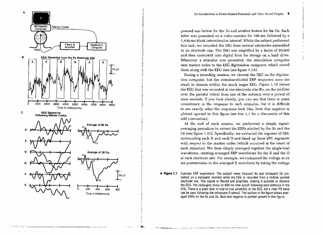
pressed one button for the XS and another button for the Os. Each letter was presented on a video monitor for 100 ms, followed by a 1,400-ms blank interstimulus intervaL While the subject performed this task, we recorded the EEG from several electrodes embedded in an electrode cap. The EEG was amplified by a factor of 20,000 and then converted into digital form for storage on a hard drive. Whenever a stimulus was presented, the stimulation computer sent marker codes to the EEG digitization computer, which stored them along with the EEG data (see figure 1.lA).

During a recording session, we viewed the EEG on the digitization computer, but the stimulus-elicited ERP responses were too small to discern within the much larger EEG. Figure 1.lB shows the EEG that was recorded at one electrode site (Pz, on the midline over the parietal lobes) from one of the subjects over a period of nine seconds. If you look closely, you can see that there is some consistency in the response to each stimulus, but it is difficult to see exactly what the responses look like. Note that negative is plotted upward in this figure (see box 1.1 for a discussion of this odd convention).

At the end of each session, we performed a simple signalaveraging procedure to extract the ERPs elicited by the Xs and the as (see figure 1.1C). Specifically. we extracted the segment of EEG surrounding each X and each a and lined up these EEG segments with respect to the marker codes (which occurred at the onset of each stimulus). We then simply averaged together the single-trial waveforms, creating averaged ERP waveforms for the X and the a at each electrode site. For example, we computed the voltage at 24 ms poststimulus in the averaged X waveform by taking the voltage

... Figura 1.1 Example ERP experiment. The subject views frequent Xs and infrequent Os presented on a computer monitor while the EEG is recorded from a midline parietal electrode site. This signal is filtered and amplified, making it possible to observe the EEG. The rectangles show an aOO-ms time epoch following each stimulus in the EEG. There is a great deal of trial-to-trial variability in the EEG, but a clear P3 wave can be seen following the infrequent 0 stimuli. The bottom of the figure shows averaged ERPs for the Xs and Os. Note that negative is plotted upward in this figure.

.II.w. ....~~~··-...",.~kll!f·o1;(.,'''*,',.

An Introduction 10 Event-Related Potentials and Their Neural Origins 11Chapter 1 10

Box 1.2 Component Naming Conventionslox 1.1 Which Way Is Up? t

tII is a common, although not universal, convention to plot ERP waveforms wlth negative voltages' upward and positive voltages downward. The sole rea l son that I plot negative upward is that this was how things were done when I joined Steve Hillyard's lab at UCSD, I once asked Steve Hillyard's mentor, Bob Galambos, how this convention came about. His answer was that that was simply that this was how things were done when he joined Hal Davis's lab at Harvard in the 1930s (see, e,g" Davis et aI., 1939; Davis, 1939). Apparently, this was a common convention for the early physiologists. Manny Donchin told me that the early neurophysiologists plotted negative upward, possibly because this allows an action potential to be plotted as an upward-going spike, and this influenced manufacturers of early EEG equipment, such as Grass. Bob Galambos also mentioned that an attempt to get everyone to agree to a uniform positive-up convention was made in the late 1960s or early 1970s, but one prominent researcher (who will remain nameless) refused to switch from negative-up to positive-up, and the whole attempt failed.

At present. some investigators plot negative upward and others plot positive upward. This is sometimes a source of confuSion, especially for people who do not regularly view ERP waveforms. and it would probably be a good idea for everyone to use the same convention (and we should probably use the same positive-up convention as the rest of the scientific world), Until this happens. plots of ERP waveforms should always make it clear which way is up.

ERP researchers should not feel too bad about this mixed up polarity problem, After all. fMRI researchers often reverse left and right when presenting brain images (due to aconvention in neurology).

measured 24 ms after each X stimulus and averaging all of these voltages together. By doing this averaging at each time point following the stimulus, we end up with a highly replicable waveform for each stimulus type.

The resulting averaged ERP waveforms consist of a sequence of positive and negative voltage deflections, which are called peaks, waves, or components. In figure 1.1C, the peaks are labeled PI, NI, P2, N2, and P3. P and N are traditionally used to indicate positive-going and negative-going peaks, respectively, and the number simply indicates a peak's position within the waveform (it

I much prefer to use nameS such as N1 and P3 rather than moo and P300, because a component's latency may vary considerably across experiments, across conditions within an experiment, or even across electrode sites within a condition. This is particularly true of the P3 wave, which almost always peaks well after300 ms (the P3 wave bad a peak latency of around 300 ms in the very firsf P3 experiment, and the name P300 has persisted despite the wide range of latencies). Moreover, in language experiments, the P3 wave generally follows the N40Q wave, making the term P300 especially problematic. Consequently, Iprefer to use a component's ordinal position in the waveform rather than its latency wilen naming it. Fortunately, the latency in milliseconds is often approximately 100 times the ordinal position, so that P1 = P100, N2 =: N200, and P3 == P300. The one obvious exception to this is the N400 component, which is often the second major negative component. For this reason, I can't seem to avoid using the time-based name N400,

is also common to give a precise latency, such as P225 for a positive peak at 225 ms), Box 1.2 further discusses the labeling conventions for ERP components. The sequence of ERP peaks reflects the flow of information through the brain.

The initial peak (Pl) is an obligatory sensory response that is elicited by visual stimuli no matter what task the subject is doing (task variations may influence Pl amplitude, but no particular task is necessary to elicit a Pl wave). In contrast, the Pl wave is strongly influenced by stimulus parameters, such as luminance. The early sensory responses are called exogenous components to indicate their dependence on external rather than internal factors. The P3 wave, in contrast, depends entirely on the task performed by the subject and is not directly influenced by the physical properties of the eliciting stimulus. The P3 wave is therefore termed an endogenous component to indicate its dependence on internal rather than external factors.

In the experiment shown in figure 1.1, the infrequent 0 stimuli elicited a much larger P3 wave than the frequent X stimuli. This is exactly what thousands of previous oddball experiments have

~ .. ~.¥~".,.,- ....""·Ii," ,j,i.',:Ui::I !!UII!i\8I!!ttt" . .",J:~.... \O;....J," ~~~~"'~~..... ,

Chapter 1 12

found. If you're just beginning to get involved in ERP research, I would recommend running an oddball experiment like this as your first experiment. It's simple to do, and you can compare your results with a huge number of published experiments.

We conducted the averaging process separately for each electrode site, yielding a separate averaged ERP waveform for each combination of stimulus type and electrode site. The P3 wave shown in figure 1.lC was largest at a midline parietal electrode site but could be seen all over the scalp. The PI wave. in contrast, was largest at lateral occipital electrode sites, and was absent over prefrontal cortex. Each ERP component has a distinctive scalp distribution that reflects the location of the patch of cortex in which it was originally generated. As I will discuss later in this chapter and in chapter 7. it is difficult to determine the location of the neural generator source simply by examining the distribution of voltage

over the scalp. Conducting an experiment like this has several steps. First, it is

necessary to attach some sort of electrodes to the subject's scalp to pick up the EEG. The EEG must be filtered and amplified so that it can be stored as a set of discrete voltage measurements on a computer. Various artifacts (e.g., eyeblinks) may contaminate the EEG, and this problem can be addressed by identifying and removing trials with artifacts or by subtracting an estimate of the artifactual activity from the EEG. Once artifacts have been eliminated, averaging of some sort is usually necessary to extract the ERPs from the overall EEG. Various signal processing techniques (e.g., digital filters) are then applied to the data to remove noise1 and isolate specific ERP components. The size and timing of the ERP components are then measured, and these measures are suhjected to statistical analyses. The following chapters will cover these technical issues in detaiL First, however, I'd like to provide an example of an experiment that was designed to answer a question of broad interest that could, in principle, be addressed by other methods but which

was well suited for ERPs.

An Introduction to Event-Related Potentials and Their Neural Origins 13

A Target = Color Target =Orientation Target = Motion

,

, ~ . i I

;,I; ! ~ I

B

·3~V

+3~V

Contra·· _.Ipsi- Time (ms)

figure 1.2 Example stimuli and data from Girelli and Luck's (1997) study. Three types of feature pop-outs were used: color, orientation, and motion. The waveforms show the averages from lateral occipital electrodes contralateral versus ipsilateral to the location of the pop-out. An N2pc component (indicated by the shaded region) can be seen as a more negative-going response between approximately 175 and 275 ms poststimulus. Negative is plotted upward. (Reprinted with permission from Luck and Girelli, 1998. © 1998 MIT Press.)

AReal Experiment Figure 1.2 illustrates an experiment that Massimo Girelli conducted in my laboratory as a part of his dissertation (for details, see Girelli & Luck. 1997). The goal of this experiment was to determine whether the same attention systems are used to detect visual search targets defined by color and by motion. As is widely known, color and motion are processed largely independently at a variety of stages within the visual system, and it therefore seemed plausible that the detection of a color-defined target would involve different attention systems than the detection of a motion-defined target. However, there is also evidence that the same cortical areas may process both the color and the motion of a discrete object, at least under some conditions, so it also seemed plausible that the same

Chapter 1 14 f

attention systems would be used to detect discrete visual search targets defined by color or by motion.

Figure 1.2A shows the stimuli that we used to address this issue. On each trial, an array was presented consisting of eight moving objects, most of which were green vertical "distractor" bars that moved downward. On 25 percent of the trials, all of the bars were distractors; on the remaining trials, one of the bars differed from the distractors in color (redl, orientation (vertical), or direction of motion (upward). We called these different bars pop-out stimuli, because they appeared to "pop out" from the otherwise homogeneous stimulus arrays. At the beginning of each trial block, the subjects were instructed that one of the three pop-out stimuli would be the target for that run, and they were told to press one button when an array contained the target and to press a different button for nontarget arrays. For example, when the horizontal bar was the target, the subjects would press one button when the array contained a horizontal pop-out and a different button when the array contained a color pop-out, a motion pop-out, or no pop-out. The main question was whether subjects would use the same attention systems .to detect each of the three types of pop-outs.

To answer this question, we needed a way to determine whether a given attention system was used for a particular type of trial. To accomplish this, we focused on an attention-related ERP component called the N2pc wave, which is typically observed for visual search arrays containing targets. The N2pc component is a negative-going deflection in the N2 latency range (200-300 ms poststimulus) that is primarily observed at posterior scalp sites contralateral to the position of the target item (N2pc is an abbreviation of N2-posterior-contralateral). Previous experiments had shown that this component reflects the focusing of attention onto a potential target item (Luck & Hillyard, 1994a, 1994b), and we sought to determine whether the attention system reflected by this component would be present for motion-defined targets as well as color- and orientation-defined targets (which had been studied previously). Thus, we assumed that if the same attention-related ERP


component was present for all three types of pop-outs, then the same attention system must be present in all three cases.

One of the most vexing issues in ERP experiments is the problem of assessing which ERP component is influenced by a given experimental manipulation. That is, the voltage recorded at any given time point reflects the sum of many underlying ERP components that overlap in time (see chapter 2 for an extended discussion of this issue). If we simply examined the ERP waveforms elicited by the color, orientation, and motion targets in this experiment, they might all have an N2 peak, but this peak might not reflect the N2pc component and might instead reflect some other neural activity that is unrelated to the focusing of attention. Fortunately, it is possible to use a trick to isolate the N2pc component (which is why we focused on this particular component). Specifically, the N2pc component is larger at electrode sites contralateral to the location of the target compared to ipsilateral sites, whereas the vast majority of ERP components would be equally large at contralateral and ipsilateral sites for these stimuli (because the overall stimulus array is bilateral). Thus, we can isolate the N2pc component by examining the difference in amplitude between the waveforms recorded from contralateral and ipsilateral electrode sites.

Figure 1.2B shows the waveforms we recorded at lateral occipital electrode sites for the three types of pop-out targets, with separate waveforms for contralateral and ipsilateral recordings. Specifically, the contralateral waveform is the average of the left hemisphere electrode site for right visual field targets and the right hemisphere site for left visual field targets, and the ipsilateral waveform is the average of the left hemisphere electrode site for left visual field targets and the right hemisphere site for right visual field t~rgets. The difference between the contralateral and ipsilateral waveforms is the N2pc wave (indicated by the shaded area),

The main finding of this experiment was that an N2pc component was present for all three types of pop-out targets. The N2pc was larger for motion pop-outs than for color or orientation popouts, which was consistent with our impression that the motion

~

Chapter I 16 An Introduction to Event-Related Potentials and Their Neural Origins 17

pop-outs seemed to attract attention more automatically than the color and orientation pop-outs. To further demonstrate that the N2pc recorded for the three types of pop-outs was actually the same ERP component in all three cases, we examined the scalp distribution of the N2pc effect (Le., the variations in N2pc amplitude across the different electrode sites). The scalp distribution was highly similar for the three pop-out types, and we therefore concluded that subjects used the same attention system across pop

out dimensions. This experiment illustrates three main points. First, the N2pc

effects shown in figure 1.2B are only about 2-3 IlV (microvolts, millionths of a volt) in size. These are tiny effects. But if we use appropriate methods to optimize the signal-to-noise ratio, we can see these tiny effects very clearly. One of the main goals of this book is to describe procedures for obtaining the best possible signal-tonoise ratio (see especially chapters 2-4).

A second important point is that this experiment uses ERP recordings as tool to address a question that is fundamentally methodology independent (Le., it is not an ERPology experiment). Although the central question of this experiment was not ERPspecific, it was a question for which ERPs were particularly well suited. For example, it is not clear how one could use purely behavioral methods to determine whether the same attention systems are used for these different stimuli, because different systems could have similar effects on behavioral output. Similarly, functional neuroimaging techniques such as PET and fMRI could be used to address this issue, but they would not be as revealing as the ERP data because of their limited temporal resolution. For example, if a given brain area were found to be active for all three pop-out types, it would not be clear whether this reflected a relatively early attention effect (such as the N2pc wave) or some higher level decision process (analogous to the P3 wave that was observed for all three pop-out types). Although the ERP data from this experiment cannot indicate which cortical region was responsible for the N2pc wave, the fact that nearly identical scalp distributions were

obtained for all three pop-out types indicates that the same cortical regions were involved, and the additional timing information provided by the ERP recordings provides further evidence that the same attention effect was present for all three pop-out types. Note also that, although it would be useful to know where the N2pc is generated, this information was not necessary for answering the main question of the experiment.

A third point this experiment illustrates is that the use of ERPs to answer cognitive neuroscience questions usually depends on previous ERPology experiments. If we did not already know that the N2pc wave is associated with the focusing of attention in visual search, we would not have been able to conclude that the same attention system was used for all three pop-out types. Consequently, the conclusions from this experiment are only as strong as the previous studies showing that the N2pc reflects the focusing of attention. Moreover, our conclusions are valid only if we have indeed isolated the same functional ERP component that was observed in previous N2pc experiments (which is likely in this experiment, given the N2pc's distinctive contralateral scalp distribution). The majority of ERP experiments face these limitations, but it is sometimes possible to design an experiment in a manner that does not require the identification of a specific ERP component. These are often the most conclusive ERP experiments, and chapter 2 describes several examples in detail.

Reliability of ERP Waveforms

Figure 1.2 shows what are called grand average ERP waveforms, which is the term ERP researchers use to refer to waveforms created by averaging together the averaged waveforms of the individual subjects. Almost all published ERP studies show grand averages, and individual-subject waveforms are presented only rarely (grand averages were less common in the early days of ERP research due to a lack of powerful computers). The use of grand averages masks the variability across subjects, which can be both a

~ 'I:

1/

Chapter 1 18

good thing (because the variability makes it difficult to see the similarities) and a bad thing (because the grand average may not accurately reflect the pattern of individual results). In either case, it is worth considering what single-subject ERP waveforms look like.

Figure 1.3 shows an example of single-subject waveforms from an N2pc experiment. The left column shows waveforms from a lateral occipital electrode site in five individual subjects (from a total set of nine subjects). As you can see, there is a tremendous amount of variability in these waveforms. Every subject has a PI peak and an NI peak, but the relative and absolute amplitudes ofthese peaks are quite different from subject to subject (compare, e.g., subjects 2 and 3). Moreover, not all of the subjects have a distinct P2 peak, and the overall voltage from 200-300 ms is positive for three subjects, near zero for one subject, and negative for one subject. This is quite typical of the variability that one sees in an ERP experiment (note that I didn't fish around for unusual examples-this is a ran

dom selection). What are the causes of this variability? To illustrate one part of

the answer to this question, the first three rows of the right side of figure 1.3 show the waveforms from a single subject who participated in three sessions of the same experiment. There is some variability from session to session, but this variability is very small compared to the variability from subject to subject. I don't know of any formal studies of the variability of the ERP waveform. but the pattern shown in figure 1.3-low within-subject variability and high between-subject variability-is consistent with my experience. A variety of factors may cause the within-subject variability, ranging from global state factors (e.g .. number of hours of sleep the previous night) to shifts in task strategy. John Polich has published an interesting series of studies showing that the P3 wave is sensitive to a variety of global factors. such as time since the last meal, body temperature. and even the time of year (see review by Polich

& Kok. 1995). There are several potential causes of between-subject variability.

One factor that probably plays a large role is the idiosyncratic fold-

I Subject 6 Subject11-~ l' \ I .... "'" \ I I Session 1

"II \ I ..........f , ' I Subject 6 Subject 2 I \ I Session 2

.... , Subject 6 Subject 3 I ........ I I ,."" , Session 3

Subject 4 .... fr=\ I I \ ~ i ~A~_m' __, 9 Subjects

Contralateral Target -----Ipsilateral Target --

-SIJV

-100 100 200 300 Time Poststimulus (ms)+SIJV

figure 1.3 Example of the reliability of averaged ERP waveforms. Data from an N2pc experiment are shown for six individual subjects (selected at random from a total set of nine subjects). Subjects 1-5 participated in a single session, and subject 6 participated in three sessions. The lower right portion of the figure shows the average of all nine subjects from the experiment. Negative is plotted upward.

J.:.

Chapler 1 20

ing pattern of the cortex. As 1 will discuss later in this chapter, the location and orientation of the cortical generator source of an ERP component has a huge influence on the size of that component at a given scalp electrode site. Every individual has a unique pattern of cortical folding, and the relationship between functional areas and specific locations on a gyrus or in a sulcus may also vary. Although I've never seen a formal study of the relationship between cortical folding patterns and individual differences in ERP waveforms, I've always assumed that this is the most significant cause of waveform variation in healthy young adults (especially in the first 250 ms). There are certainly other factors that can influence the shape of the waveforms, including drugs, age, psychopathology, and even personality. But in experiments that focus on healthy young adults, these factors probably playa relative small role.

The waveforms in the bottom right portion of figure 1.3 represent the grand average of the ·nine subjects in this experiment. A striking attribute of the grand average waveforms is that the peaks are smaller than those in most of the single-subject waveforms. This might seem odd, but it is perfectly understandable. The time point at which the voltage reaches its peak values for one subject are not the same as for other subjects, and the peaks in the grand averages are not at the same time as the peaks for the individual subjects. Moreover, there are many time points at which the voltage is positive for some subjects and negative for others. Thus. the grand average is smaller overall than most of the individual-subject waveforms. This is a good example of how even simple data processing procedures can influence ERP waveforms in ways that may be unexpected.

There are studies showing that if you average together the pictures of a hundred randomly selected faces, the resulting average face is quite attractive and looks the same as any other average of a hundred randomly selected faces from the same population. In my experience, the same is true for ERP waveforms: Whenever I run an experiment with a given set of stimuli, the grand average of ten to fifteen subjects is quite attractive and looks a lot like the


grand average of ten to fifteen different subjects in a similar experiment. Of course the waveform will look different if the stimuli or task differ substantially between experiments, and occasionally you will get several subjects with odd-looking waveforms that make the grand average look a little odd. But usually you will see a lot of similarity in the grand averages from experiment to experiment.

Advantages and Disadvantages of the ERP Technique

Comparison with Behavioral Measures When ERPs were first used to study issues in the domain of cognitive neuroscience, they were primarily used as an alternative to measurements of the speed and accuracy of motor responses in paradigms with discrete stimuli and responses. In this context, ERPs have two distinct advantages. First, an overt response reflects the output of a large number of individual cognitive processes, and variations in reaction time (RT) and accuracy are difficult to attribute to variations in a speCific cognitive process. ERPs, in contrast, provide a continuous measure of processing between a stimulus and a response, making it possible to determine which stage or stages of processing are affected by a specific experimental manipulation. As an example, consider the Stroop paradigm, in which subjects must name the color of the ink in which a word is drawn. Subjects are slower when the word is incompatible with the ink color than when the ink color and word are the same (e.g., subjects are slower to say "green" when presented with the word "red" drawn in green ink than when they are presented with the word "green" drawn in green ink). Do these slowed responses reflect a slowing of perceptual processes or a slowing of response processes? It is difficult to answer this question simply by looking at the behavioral responses, but studies of the P3 wave have been very useful in addressing this issue. Specifically, it is well

'0.

Chapter 1 22

documented that the latency of the P3 wave becomes longer when perceptual processes are delayed. but several studies have shown that P3 latency is not delayed on incompatible trials in the Stroop paradigm. indicating that the delays in RT reflect delays in some postperceptual stage (see. e.g .• Duncan-Johnson & Kopell, 1981). Thus, ERPs are very useful for determining which stage or stages of processing are influenced by a given experimental manipulation (for a detailed set of examples. see Luck, Woodman. & Vogel, 2000).

A second advantage of ERPs over behavioral measures is that they can provide an online measure of the processing of stimuli even when there is no behavioral response. For example. much of my own research involves comparing the processing of attended versus ignored stimuli, and ERP recordings make it possible to monitor "covertly" the processing of the ignored stimuli without requiring subjects to respond to them. Similarly. ERP studies of language comprehension can assess the processing of a word embedded in the middle of a sentence at the time the word is presented rather than relying on a response made at the end of the sentence. Thus, the ability to covertly monitor the online processing of information is one of the greatest advantages of the ERP technique. For these reasons, I like to refer to the ERP techniq"!le as "reaction time for the twenty-first century." ..

ERP recordings also have some disadvantages compared to behavioral measures. The most obvious disadvantage is that the functional significance of an ERP component is virtually never as clear as the functional significance of a behavioral response. In most cases, we do not know the specific biophysical events that underlie the production of a given ERP response or the consequences of those events for information processing. In contrast. when a computer records a button-press response. we have a much clearer understanding of what that signal means. For example. when the reaction time (RT) in condition A is 30 ms longer than the RT in condition B, we know that the amount of time required to encode, process, and act on the stimuli was 30 ms longer in condition A than in condition B. In contrast. when the peak latency of an ERP


component is 30 ms later in condition A than in condition B. we can draw no conclusions without relying on a long chain of assumptions and inferences (see chapter 2 for a discussion of some problems associated with measuring ERP latencies). Some amount of inference is always necessary when interpreting physiological measures of cognition. but some measures are easier to interpret than others. For example. when we record an action potential, we have an excellent understanding of the biophysical events that produced the action potential and the role that action potentials play in information processing. Thus, the basic signal is more difficult to interpret in ERP experiments than in behavioral experiments or in single-unit recordings (but probably no more difficult to interpret than the BOLD [blood oxygen level-dependent] signal in fMRI experiments).

A second disadvantage of the ERP technique is that ERPs are so small that it usually requires a large number of trials to measure them accurately. In most behavioral experiments, a reaction time difference can be observed with only about twenty to thirty trials per subject in each condition, whereas ERP effects often require fifty. a hundred, or even a thousand trials per subject in each condition. I have frequently started designing an ERP experiment and then given up when I realized that the experiment would require ten hours of data collection from each subject. Moreover, I rarely conduct an experiment that requires less than three hours of data collection from each subject. This places significant limitations on the types of questions that ERP recordings can realistically answer. For example, there are some behavioral experiments in which a given subject can receive only one trial in each condition (e.g., the inattentional blindness paradigm); experiments of this nature are not practical with ERP recordings.

Comparisen with Other Pbysiological Measures Table 1.1 compares the ERP technique (along with its magnetic counterpart, the event-related magnetic field, or ERMF, technique)

ik

Chapter 1 24

Table 1.1 Comparison of invasiveness. spatial resolution. temporal resolution. and cost for microelectrode measures (single-unit and local field-potential recordings), hemodynamic measures (PET and fMRI), and electromagnetic measures (ERPs and ERMFs)

MICROELECTRODE HEMODYNAMIC ELECTROMASNETIC

MEASURES MEASURES MEASURES

Invasiveness Poor Good (PET) Excellent Excellent (fMRI)

Spatial resolution Excellent Good Undefined/poor (ERPs) Undefined/better (ERMFs)

Temporal resolution Excellent Poor Excellent

Cost Fairly Expensive (PET) Inexpensive (ERPs) expensive Expensive (fMRI) Expensive (ERMFs)

, with several other phYSiological recording techniques along four major dimensions: invasiveness. spatial resolution, temporal resolution, and cost. The other classes of techniques considered are microelectrode measures (single-unit, multi-unit, and local field potential recordings) and hemodynamic measures (PET and fMRl).

Invasiveness Microelectrode measures require inserting an electrode into the brain and are therefore limited to nonhuman species (or. in rare cases, human neurosurgery patients). The obvious disadvantage of primate recordings is that human brains are different from primate brains. The less obvious disadvantage is that a monkey typically requires months of training to be able to perform a task that a human can learn in five minutes, and once a monkey is trained. it usually spends months performing the tasks while recordings are made. Thus, monkeys are often highly overtrained and probably perform tasks in a manner that is different from the prototypical naive college sophomore. This can make it difficult

An mtrod uction to Event -Related Potentials and Their Neural Origins 25

to relate monkey results to the large corpus of human cognitive experiments. PET experiments are also somewhat problematic in terms of invasiveness. To avoid exposing subjects to excessive levels of radiation. each subject can be tested in only a small number of conditions. In contrast. there is no fundamental restriction on the amount of ERP or fMRI data that can be collected from a single subject.

Spatial and Temporal Resolution Many authors have noted that electromagnetic measures and hemodynamic measures have complementary patterns of spatial and temporal resolution. with high temporal resolution and poor spatial resolution for electromagnetic measures and poor temporal resolution and high spatial resolution for hemodynamic measures. ERPs have a temporal resolution of 1 ms or better under optimal conditions. whereas hemodynamic measures are limited to a resolution of several seconds by the sluggish nature of the hemodynamic response. This is over a thousandfold difference. and it means that ERPs can easily address some questions that PET and fMRI cannot hope to address. However, hemodynamic measures have a spatial resolution in the millimeter range. which electromagnetic measures cannot match (except, perhaps. under certain unusual conditions). In fact, as I will discuss in greater detail later in this chapter and in chapter 7, the spatial resolution of the ERP technique is fundamentally undefined. because there are infinitely many internal ERP generator configurations that can explain a given pattern of ERP data. Unlike PET and flvIRl. it is not currently possible to specify a margin of error for an ERP localization claim (for the typical case, in which several sources are simultaneously active). That is. with current techniques. it is impossible to know whether a given localization estimate is within some specific number of millimeters from the actual generator source. It may someday be possible to definitively localize ERPs, but at present the spatial resolution of the ERP technique is simply undefined.

&..

Chapter 1 26

The fact that ERPs are not easily localized has a consequence that is not often noted. Specifically, the voltage recorded at any given moment from a single electrode reflects the summed contributions from many different ERP generator sources, each of which reflects a different neurocognitive process. This makes it extremely difficult to isolate a single ERP component from the overall ERP waveform. This is probably the single greatest shortcoming of the ERP technique, because if you can't isolate an ERP component with confidence, it is usually difficult to draw strong conclusions. Chapter 2 will discuss this issue in greater detaiL

Cost ERPs are much less expensive than the other techniques listed in table 1,1. It is possible to equip a good ERP lab for less than US $50,000, and the disposable supplies required to test a single subject are very inexpensive (US $1-3). A graduate student or an advanced undergraduate can easily carry out the actual recordings, and the costs related to storing and analyzing the data are minimaL These costs have dropped a great deal over the past twenty years, largely due to the decreased cost of computing equipment. FMRI is fairly expensive, the major costs being personnel and amortization of the machine. One session typically costs US $300-800. PET is exorbitantly expensive. primarily due to the need for radioactive isotopes with short half-lives and medical personneL Single-unit recordings are also fairly expensive due to the per diem costs of maintaining the monkeys, the cost of the surgical and animal care facilities, and the high level of expertise required to record electro physiological data from awake. behaving

monkeys.

Choosing the Right QuestiOns Given that the ERP technique has both significant advantages and significant disadvantages, it is extremely important to focus ERP experiments on questions for which ERPs are well suited. For example, ERPs are particularly useful for addressing questions about


which neurocognitive process is influenced by a given manipulation. Conversely, ERPs are poorly suited for asking questions that require neuroanatomical specificity (except under certain special conditions; see chapter 7). In addition, it is very helpful to ask questions that can be addressed with a component that is relatively easy to isolate (such as the N2pc component and the lateralized readiness potential) or questions that avoid the problem of identifying a specific ERP component altogether. Unfortunately, there are no simple rules for determining whether a given question can be easily answered with ERPs, but chapter 2 discusses a number of general principles.

The Neural Origins of ERPs

Basic Electrical Concepts Before reading this section, I would encourage you to read the appendix, which reviews a few key principles of electricity and magnetism. You probably learned this material in a physics class several years ago, but it's worthwhile to review it again in the context of ERP recordings. You should definitely read it if (al you're not quite sure what the difference between current and voltage is; or (b) you don't know Ohm's law off the top of your head. The appendix is, I admit, a bit boring. But it's short and not terribly complicated.

Electrical Activity In Neurons To understand the nature of the voltages that can be recorded at the scalp, it is necessary to understand the voltages that are generated inside the brain. There are two main types of electrical activity associated with neurons, action potentials and postsynaptic potentials. Action potentials are discrete voltage spikes that travel from the beginning of the axon at the cell body to the axon terminals,

An Introduction to Event-Related Potentials and Their Neural Origins 29Chapter 1 28

other), action potentials in different axons will typically cancel, where neurotransmitters are released. Postsynaptic potentials are the voltages that arise when the neurotransmitters bind to recep and the only way to record the action potentials from a large

number of neurons is to place the electrode near the cell bodies tors on the membrane of the postsynaptic cell, causing ion chanand to use a very high impedance electrode that is sensitivenels to open or close and leading to a graded change in the only to nearby neurons. As a result, ERPs reflect postsynaptic potential across the cell membrane. If an electrode is lowered into potentials rather than action potentials (except under extremely

can be recorded. It is fairly easy to isolate the action potentials the intercellular space in a living brain, both types of potentials

rare circumstances).

arising from a single neuron by inserting a micro electrode into the brain, but it is virtually impossible to completely isolate a single neuron's postsynaptic potentials in an in vivo extracellular Summation of Postsynaptic Potentials

Whereas the duration of an action potential is only about arecording. Consequently, in vivo recordings of individual neurons millisecond, postsynaptic potentials typically last tens or even

postsynaptic potentials. When recording many neurons simultane hundreds of milliseconds. In addition, postsynaptic potentials are

ously, it is possible to measure either their summed postsynaptic largely confined to the dendrites and cell body and occur essen

potentials or their action potentials. Recordings of action potentials tially instantaneously rather than traveling down the axon at a

from large populations of neurons are called multi-unit recordings, fixed rate. Under certain conditions, these factors allow postsynap

and recordings of postsynaptic potentials from large groups of neu tic potentials to summate rather than cancel, making it possible to record them at a great distance (i.e., at the scalp).

("single-unit" recordings) measure action potentials rather than

rons are called local field potential recordings. In the vast majority of cases, surface electrodes cannot detect Very little research has examined the biophysical events that

action potentials due to the timing of the action potentials and the give rise to scalp ERPs, but figure 1.4 shows the current best guess.

physical arrangement ofaxons. When an action potential is gener If an excitatory neurotransmitter is released at the apical dendrites

ated, current flows rapidly into and then out of the axon at one of a cortical pyramidal cell, as shown in figure 1.4A, current will

point along the axon, and then this same inflow and outflow occur flow from the extracellular space into the cell, yielding a net nega

-

at the next point along the axon, and so on until the action poten tivity on the outside of the cell in the region of the apical den

tial reaches a terminal. If two neurons send their action potentials drites. To complete the circuit, current will also flow out of the

down axons that run parallel to each other, and the action poten cell body and basal dendrites, yielding a net positivity in this area.

tials occur at exactly the same time, then the voltages from the two Together, the negativity at the apical dendrites and the positivity at

neurons will summate and the voltage recorded from a nearby the cell body create a tiny dipole (a dipole is simply a pair of posi

electrode will be approximately twice as large as the voltage tive and negative electrical charges separated by a small distance).

recorded from a single action potential. However, if one neuron The dipole from a single neuron is so small that it would be

fires slightly after the other, then current at a given spatial location impossible to record it from a distant scalp electrode, but under

will be flowing into one axon at the same time that it is flowing out certain conditions the dipoles from many neurons will summate,

of the other axon, so they cancel each other and produce a much making it possible to measure the resulting voltage at the scalp.

smaller signal at the nearby electrode. Because neurons rarely For the summated voltages to be recordable at the scalp, they must

fire at precisely the same time (i.e., within microseconds of each occur at approximately the same time across thousands or millions

i.

A \\.,..-J)~ \g:'L /I

y

Chapter 1 30

H~HtHH'...1' (...\Jnn:;:n~ + "* I i-1 + ..... I ..

.... + +" ! " + ~ I "B .... + .... ! ....f.'"'"'''T~'+ t'4 f ,....

Stimulated ""l. .. Region

of Cortex

c

postSyna~ell Axon

+ +-._. Magnetic Magnetic Field

Field Leaving Head

Magnetic Field Entering Head

o ~ E

\ Current Dipole

Principles of ERP generation. (A) Schematic pyramidal cell during neurotransmisFigure 1.4 sion. An excitatory neurotransmitter is released from the presynaptic terminals, causing positive ions to flow into the postsynaptic neuron. This creates a net negative extracellular voltage (represented by the" -" symbols) in the area of other parts of the neuron, yielding a small dipole. (B) Folded sheet of cortex containing many pyramidal cells. When a region of this sheet is stimulated, the dipoles from the individual neurons summate. (e) The summated dipoles from the individual neurons can be approximated by a single equivalent current dipole, shown here as an arrow. The position and orientation of this dipole determine the distribution of positive and


of neurons, and the dipoles from the individual neurons must be spatially aligned. If the neurons are at random orientations with respect to each other, then the positivity from one neuron may be adjacent to the negativity from the next neuron, leading to cancellation. Similarly, if one neuron receives an excitatory neurotransmitter and another receives an inhibitory neurotransmitter, the dipoles of the neurons will be in opposite directions and will cancel. However, if the neurons all have a similar orientation and all receive the same type of input, their dipoles will summate and may be measurable at the scalp. This is most likely to occur in cortical pyramidal cells, which are aligned perpendicular to the surface of the cortex, as shown in figure 1.4B.

The summation of the individual dipoles is complicated by thl'l fact that the cortex is not flat, but instead has many folds. Fortunately, however, physicists have demonstrated that the summation of many dipoles is essentially equivalent to a single dipole formed by averaging the orientations of the individual dipoles.2 This averaged dipole is called an equivalent current dipole (ECD). It is important to note, however, that whenever the individual dipoles are more than 90 degrees from each other, they will cancel each other to some extent, with complete cancellation at 180 degrees. For example, the Purkinje cells in the cerebellar cortex are beautifully aligned with each other and oriented perpendicular to the cortical surface. but the cortical surface is so highly folded that the dipoles in one small patch of cerebellar cortex will almost always be cancelled by dipoles in a nearby but oppositely oriented patch, making it difficult or impossible to record cerebellar activity from the scalp.

Figure 1.4 (continued) negative voltages recorded at the surface of the head. (D) Example of a current dipole with a magnetic field traveling around it. (E) Example ot the magnetic field generated by a dipole that lies just inside the surface of the skull. If the dipole is roughly parallel to the surface, the magnetic field can be recorded as it leaves and enters the head; no field can be recorded if the dipole is oriented radially. Reprinted with permiSSion tram Luck and Girelli 1998. (© 1998 MIT Press.)

Chapter 1 32

Volume Conduction When a dipole is present in a conductive medium such as the brain, current is conducted throughout that medium until it reaches the surface. This is called volume conduction and is illustrated in figure 1.4C. The voltage that will be present at any given point on the surface of the scalp will depend on the position and orientation of the generator dipole and also on the resistance and shape of the various components of the head (most notably the brain, the skull, and the scalp; the eye holes also have an influence, especially for ERP activity generated in prefrontal cortex).

Electricity does not just run directly between the two poles of a dipole in a conductive medium, but instead spreads out through the conductor. Consequently, ERPs spread out as they travel through the brain. In addition, because electricity tends to follow the path of least resistance, ERPs tend to spread laterally when they encounter the high resistance of the skull. Together, these two factors greatly blur the surface distribution of voltage, and an ERP generated in one part of the brain can lead to substantial voltages at quite distant parts of the scalp. There are algorithms that can reduce this blurring, either by estimating the flow of current or by deblurring the voltage distribution to estimate the voltage distribution that is present on the brain's surface (Gevins et a1., 1999; Pernier, Perrin, & Bertrand, 1988). These algorithms can be very useful, although you should remember that they only eliminate one source of blurring (the skull) and do not indicate the

actual generator location of the ERPs. Another important point is that electricity travels at nearly the

speed of light. For all practical purposes, the voltages recorded at the scalp reflect what is happening in the brain at the same mo

ment in time.

Magnetic fields The blurring of voltage caused by the high resistance of the skull can be largely circumvented by recording magnetic fields instead


of electrical potentials. As figure 1.4D illustrates, an electrical dipole is always surrounded by a magnetic field, and these fields summate in the same manner as voltages. Thus. whenever an ERP is generated, a magnetic field is also generated, running around the ERP dipole. Moreover, the skull is transparent to magnetism,3 and the magnetic fields are not blurred by the skull, leading to much greater spatial resolution than is possible with electrical potentials. The magnetic equivalent of the EEG is called the magnetoencephalogram (MEG), and the magnetic equivalent of an ERP is an eventrelated magnetic field (ERMF).

As figure 1.4E illustrates, a dipole that is parallel to the surface of the scalp will be accompanied by a magnetic field that leaves the head on one side of the dipole and enters back again on the other side. If you place a highly sensitive probe called a SQUID (super-conducting quantum interference device) next to the head, it is possible to measure the magnetic field as it leaves and reenters the head. Because magnetic fields are not as smeared out as electrical potentials, they can provide more precise localization. However, as chapter 7 will discuss, the combination of ERP and ERMF recordings proVides even better localization than ERMF recordings alone. Unfortunately, magnetic recordings are very expensive because supercooling is expensive and because an expensive magnetically shielded recording chamber is necessary to attenuate the Earth's relatively large magnetic field.

ERP Localization If I tell you the locations and orientations of a set of dipoles in a volume with a known distribution of conductances, then it would be possible for you to use a set of equations to compute the distribution of voltage that would be observed for those dipoles. This is called the forward problem, and it is relatively easy to solve. However, if I provide you with an observed voltage distribution and ask you to tell me the locations and orientations of the dipoles, you will not be able to provide an answer. This is called the inverse

~

Chapter 1 34

problem, and it is what mathematicians call an "ill-posed" or "underdetermined" problem. This simply means that there is not just one set of dipoles that can explain a given voltage distribution. In fact, researchers have known for over 150 years that an infinite number of different dipole configurations can produce any given voltage distribution (Helmholtz, 1853) (see also Nunez, 1981; Plonsey, 1963). Thus, it is impossible to know with certainty which one of these configurations is the one that is actually responsible for producing the observed voltage distribution.

It is possible to use additional constraints to overcome the illposed nature of the inverse problem. However, there is currently no mathematical technique that is widely accepted as providing a foolproof means of localizing ERP generator sources. By foolproof, I mean a technique that can provide a reasonably small and welljustified margin of error, making it possible to provide a p-value or likelihood ratio for a statement about the anatomical location of an ERP effect. For example, I would like to be able to say that the N2pc component in a particular experiment was generated within 12 mm of the fusiform gyrus and that the probability that this localization is incorrect is less than .05. I am aware of no mathematical localization technique that allows one to make such statements.

As discussed earlier in this chapter, the main advantages of the ERP technique are its high temporal resolution, its relatively low cost, its noninvasiveness, and its ability to provide a covert and continuous measure of processing. Spatial resolution is simply not one of the strengths of the ERP technique, and it seems appropriate to use this technique primarily to address issues that take advantage of its strengths and are not limited by its weaknesses.

Chapter 7 provides more details about ERP localization.

;ummary of Major ERP Components This section provides a brief description of the ERP components commonly encoUlltered in cognitive neuroscience research. Some


of these components could justify an entire chapter, but I will cover just the basics. For more extensive descriptions, see reviews by Coles and Rugg (1995), Hillyard and Picton (1987), Picton and Stuss (1980), NaiWinen and Picton (1986), and Regan (1989).

Before I start describing the components, however, I'd like to clarify something that is often confusing to ERP newcomers. Specifically, ERP components are usually given labels such as Pl and Nl that refer to their polarity and position within the waveform, and one must be careful not to assume that these labels are linked somehow to the nature of the underlying brain activity. Most notably, sensory components from different modalities that are given the same label are not usually related in any functional manner: They just happen to have the same polarity and ordinal position in the waveform. For example, the auditory PI and Nl components bear no particular relationship to the visual P1 and N1 components. Some late components such as the P3 wave are largely modality-independent, but even the P3 wave may have modalityspecific subcomponents (see, e.g., Luck & Hillyard, 1994a). Even within a single modality, a component labeled N2 in one experiment may not be the same as a component labeled N2 in another experiment. Some researchers use a bar over the latency of a component (e.g., P300) when they are referring to a theoretical entity rather than simply labeling the observed polarity and latency of a peak from a particular experiment.

Visual Sensory Responses

C1 The first major visual ERP component is usually called the C1 wave, and it is largest at posterior midline electrode sites. Unlike most other components, it is not labeled with a P or an N because its polarity can vary. The Cl wave appears to be generated in area VI (primary visual cortex), which in humans is folded into the calcarine fissure. The part of area V1 that codes the lower visual field

Chapter 1 36

is on the upper bank of the fissure and the part that codes the upper visual field is on the lower bank. As a result. the voltage recorded on the scalp above the calcarine fissure is positive for stimuli in the lower visual field and negative for stimuli in the upper visual field (Clark. Fan, & Hillyard, 1995; Jeffreys & Axford, 1972). The CI wave is small or positive for stimuli on the horizontal midline, causing it to summate with the PI wave into a single wave. Consequently, a distinct Cl wave is usually not observed unless upper-field stimuli are used to generate a negative Cl wave (which can be easily distinguished from the positive PI wave). The Cl wave typically onsets 40-60 ms poststimulus and peaks 80-100 ms poststimulus, and it is highly sensitive to stimulus parameters,

such as contrast and spatial frequency.

P1 The Cl wave is followed by the PI wave, which is largest at lateral occipital electrode sites and typically onsets 60-90 ms poststimulus with a peak between 100-130 ms. Note, however, that P1 onset time is difficult to assess accurately due to overlap with the Cl wave. In addition, PI latency will vary substantially depending on stimulus contrast. A few studies have attempted to localize the IPI wave by means of mathematical modeling procedures. sometimes combined with co-localization with fMRI effects, and these studies suggest that the early portion of the PI wave arises from dorsal extrastriate cortex (in the middle occipital gyrus), whereas a later portion arises more ventrally from the fusiform gyrus (see Di Russo et aI., 2002). Note, however, that at least thirty distinct visual areas are activated within the first 100 ms after the onset of a visual stimulus, and many of these areas presumably contribute to the voltages recorded in the C1 and PI latency range. Like the C1 wave, the PI wave is sensitive to a variations in stimulus parameters, as would be expected given its likely origins in extra striate visual cortex. The PI wave is also sensitive to the direction of spatial attention (see review by Hillyard, Vogel, & Luck. 1998) and to the subject's state of arousal (Vogel & Luck, 2000). Other top-down variables do not appear to reliably iufluence tbe PI wave.

An Introduction to Event-J:{elated Potentials and Their Neural Origins 37

N1 The PI wave is followed by the Nl wave. There are several visual N1 subcomponents. The earliest subcomponent peaks 100150 ms poststimulus at anterior electrode sites, and there appear to be at least two posterior N1 components that typically peak 150-200 ms poststimulus. one arising from parietal cortex and another arising from lateral OCcipital cortex. Many studies have shown that spatial attention influences these components (see reviews by Hillyard et aI., 1998; Mangun. 1995). In addition. the lateral occipital N1 subcomponent appears to be larger when subjects are performing discrimination tasks than when they are performing detection tasks, which has led to the proposal that thi~ subcomponent reflects discriminative processing of some sort (Hopf et ai., 2002; Ritter et aI., 1979; Vogel & Luck, 2000).

P2 A distinct P2 wave follows the Nl wave at anterior and central scalp sites. This component is larger for stimuli containing target features. and this effect is enhanced when the targets are relatively infrequent (see Luck & Hillyard, 1994a). In this sense, the anterior P2 wave is similar to the P3 wave. However, the anterior P2 effects occur only when the target is defined by fairly simple stimulus features. whereas P3 effects can occur for arbitrarily complex target categories. At posterior sites, the P2 wave is often difficult to distinguish from the overlapping N1, N2, and P3 waves. Consequently, not much is known about the posterior P2 wave.

N170 and Vertex Positive Potential Jeffreys (1989) compared the responses to faces and non-face stimuli, and he found a difference between 150 and 200 ms at central midline sites that he named the vertex positive potential (the electrode site at the very top of the head is sometimes called the vertex site). Jeffreys noted that this effect inverted in polarity at more lateral sites, but he did not have any recordings from electrode sites over inferotemporal cortex. More recent studies from other laboratories that used a broader range of electrode sites have found that faces elicit a more negative potential than non-face stimuli at lateral occipital electrode sites,

Chapter 1 38

especially over the right hemisphere, with a peak at approximately 170 ms (Bentin et al., 1996; Rossion et al., 1999). This effect is typically called the N170 wave. It is likely that the N170 and the vertex positive potential are just the opposite sides of the same dipole (although this is not a hundred percent certain-see George et aI., 1996; Rossion et al., 1999).

The N170 is later and/or larger for inverted faces than for upright faces, a hallmark of face specialization. However, an inversion effect is also observed for non-face stimuli when the subjects have extensive experience viewing these stimuli in an upright orientations (Rossion et aI., 2002). Moreover, other studies have shown that the vertex positive potential (and presumably the

also occurs for other highly familiar stimuli, such as words (Schendan, Ganis. & Kutas, 1998). But the face specificity of the N170 is still a topic of considerable debate (Bentin & Carmel, 2002; Carmel & Bentin, 2002; Rossion, Curran, & Gauthier, 2002).

Auditory Sensory Responses

Very Early Components Under appropriate conditions, it is possible to observe a sequence of ERP peaks within the first 10 ms of the onset of an auditory stimulus. Various sources of evidence indicate that these peaks arise from various stages along the brainstem auditory pathways, and these peaks are therefore called the brainstem evoked responses (BERs) or auditory brainstem responses (ABRs). BERs are extremely useful for assessing auditory pathology, especially in infants. When my children were born, they were both given BER screening tests, and it was gratifying to see that a variant of my main research technique is used for such an important clinical application. The BERs are followed by the midlatency components (defined as' responses between 10 and 50 ms), which probably arise at least in part from the medial geniculate nucleus and the primary auditory cortex. Attention has its first reliable effects in the midlatency range, but I don't know of any other top

_._-.,.,,,...'"',._.


down variables that influence auditory activity in this time range. The midlatency components are followed by the auditory Pl wave (ca. 50 ms). which is typically largest at frontocentral electrode sites.

N1 Like the visual Nl wave, the auditory Nl wave has several distinct subcomponents (see review by NiiiWinen & Picton, 19B7). These include (1) a frontocentral component that peaks around 75 ms and appears to be generated in the auditory cortex on the dorsal surface of the temporal lobes, (2) a vertex-maximum potential of unknown origin that peaks around 100 ms, and (3) a mOre laterally distributed component that peaks around 150 ms and appears to be generated in the superior temporal gyrus. Further fractionation of the auditory Nl wave is possible (see, e.g., Alcaini et aL, 1994). The Nl wave is sensitive to attention. Although some attention effects in the Nl latency range reflect the addition of an endogenous component, attention can influence the Nl wave itself [or at least some Nl subcomponents) (Woldorff et aI., 1993).

Mismatch Negativity The mismatch negativity (MMN) is observed when subjects are exposed to a repetitive train of identical stimuli with occasional mismatching stimuli (e.g., a sequence with many BOO-Hz tones and occasional 1200-Hz tones). The mismatching stimuli elicit a negative-going wave that is largest at central midline scalp sites and typically peaks between 160 and 220 ms. Several other components are sensitive to mismatches if they are task-relevant. but the MMN is observed even if subjects are not using the stimulus stream for a task (e.g., if they are reading a book while the stimuli are being presented). However. the MMN can be eliminated for stimuli presented in one ear if the subjects focus attention very strongly on a competing sequence of stimuli in the other ear (Woldorff, Hackley, & Hillyard, 1991). The MMN is thought to reflect a fairly automatic process that compares incoming stimuli to a sensory melllory trace of preceding stimuli. '

An Introduction to Event-Related Potentials and Their Neural Origins 41Chapter 1 40

Somatosensory, Olfactory, and Gustatory Responses The vast majority of cognitive ERP experiments use auditory or visual stimuli, so I will provide only a brief mention of components from other modalities. The response to a somatosensory stimulus begins with one of the rare ERP components (sometimes called NlO) that reflects action potentials rather than postsynaptic potentials, arising from the peripheral nerves. This is followed by a set of subcortical components (ca. 10-20 ms) and a set of short- and medium-latency cortical components (ca. 20-100 ms). An N1 wave is then observed at approximately 150 ms. followed by a P2 wave at approximately 200 ms (together, these two peaks are somec

times called the vertex potential). It is difficult to record olfactory and gustatory ERP responses,

largely because it is difficult to deliver precisely timed, suddenonset stimuli in these modalities (which is neGessary when computing averaged ERP waveforms). However, recent studies have shown that these potentials can be recorded when using appropriate stimulation devices (see, e.g .. Ikui, 2002; Wada. 1999).

The 12 family The N2 time range has been well studied, and researchers have identified many clearly different components in this lime range (see extensive discussions in Luck & Hillyard, 1994a; Niiiitiinen &

Picton, 1986). As NiilHiinen and Picton (1986) describe, a repetitive, nontarget stimulus will elicit an N2 deflection that can be thought of as the basic N2 (although it doubtless contains several subcomponents). If other stimuli (often called deviants) are occasionally presented within a repetitive train, a larger amplitude is observed in the N2 latency range. If these deviants are taskirrelevant tones, this effect will consist of a mismatch negativity (visual mismatches do not seem to elicit exactly this sort of automatic mismatch response). If the deviants are task-relevant, then a somewhat later N2 effect is also observed, called N2b (the mis

match negativity is sometimes called N2a). This component is larger for less frequent targets, and it is thought to be a sign of the stimulus categorization process. Both auditory and visual deviants will, if task-relevant, elicit an N2b component, but this effect is largest over central sites for auditory stimuli and over posterior sites for visual stimuli (Simson, Vaughan, & Ritter, 1977). We do not really know if the auditory and visual N2b components represent homologous neural processing functions.

In the visual domain, deviance is often studied spatially rather than temporally. That is, rather than examining the response to a deviant item presented within a temporal sequence of homogeneous items, one can compare the ERP waveform elicited by a simultaneous array of homogeneous items to the ERP waveform elicited by a simultaneous array that contains several identical items plus one deviant item. When this is done, one can distinguish three N2 components (Luck & Hillyard, 1994a). The first is a bilateral, anterior response that is present even when the deviant item is not a target (but it is not as automatic as the MMN because it is not present unless subjects are looking for deviant targets of some sort). This is followed by two posterior N2 subcomponents that are present only if the deviant item is a target (or resembles the target at first glance). One of these subcomponents is the standard N2b wave, which is bilateral and probability sensitive. The second is called N2pc, where the pc is an abbreviation of posterior contralateral, denoting the fact that this component is observed at posterior electrode sites contralateral to the location of the target. The N2pc component is not probability sensitive, and it reflects the focusing of spatial attention onto the target location (and possibly the suppression of the surrounding nontarget items-see Eimer, 1996; Luck et aI., 1997; Luck & Hillyard. 1994b). A contralateral negativity is also observed during visual working memory tasks, but it has a more parietally focused scalp distribution and appears to retIeet some aspect of working memory maintenance (Vogel &

Machizawa, 2004).

il

1 An Introduction to Event-Related Potentials and Their ...

Documents

Transcript of 1 An Introduction to Event-Related Potentials and Their ...