1 An ensemble data set of sea-surface temperature change ...
146
Confidential manuscript submitted to Journal of Geophysical Research Atmospheres 1 An ensemble data set of sea-surface temperature change from 1850: the Met Office 1 Hadley Centre HadSST.4.0.0.0 data set 2 Enter authors here: J.J. Kennedy 1 , N.A. Rayner 1 , C.P. Atkinson 1 , R.E. Killick 1 3 1 Met Office Hadley Centre, Exeter, UK. 4 Corresponding author: John Kennedy ([email protected]) 5 Key Points: 6 We describe the construction of HadSST.4.0.0.0, a climate data set of sea-surface 7 temperature change from 1850 to 2018. 8 A range of bias adjustments was generated to create an ensemble of SST data sets with 9 the ensemble spread partly constrained by oceanographic profile measurements. 10 New estimates reduce discrepancy between data sets during the mid 20 th century and the 11 recent slowdown in warming, but highlight a divergence in the early 1990s. 12 13
Transcript of 1 An ensemble data set of sea-surface temperature change ...

Confidential manuscript submitted to Journal of Geophysical Research Atmospheres
1
An ensemble data set of sea-surface temperature change from 1850: the Met Office 1
Hadley Centre HadSST.4.0.0.0 data set 2
Enter authors here: J.J. Kennedy1, N.A. Rayner
1, C.P. Atkinson
1, R.E. Killick
1 3
1Met Office Hadley Centre, Exeter, UK. 4
Corresponding author: John Kennedy ([email protected]) 5
Key Points: 6
We describe the construction of HadSST.4.0.0.0, a climate data set of sea-surface 7
temperature change from 1850 to 2018. 8
A range of bias adjustments was generated to create an ensemble of SST data sets with 9
the ensemble spread partly constrained by oceanographic profile measurements. 10
New estimates reduce discrepancy between data sets during the mid 20th
century and the 11
recent slowdown in warming, but highlight a divergence in the early 1990s. 12
13
Confidential manuscript submitted to Journal of Geophysical Research Atmospheres
2
Abstract (max 250 words) 14
One of the largest sources of uncertainty in estimates of global temperature change is that 15
associated with the correction of systematic errors in sea-surface temperature (SST) 16
measurements. Despite recent work to quantify and reduce these errors throughout the historical 17
record, differences between analyses remain larger than can be explained by the estimated 18
uncertainties. 19
We revisited the method used to estimate systematic errors and their uncertainties in version 3 of 20
the Met Office Hadley Centre SST data set, HadSST. Using comparisons with oceanographic 21
temperature-profiles, we make estimates of biases associated with engine-room measurements 22
and insulated buckets and constrain the ranges of two of the more uncertain parameters in the 23
bias estimation: the timing of the transition from uninsulated to insulated buckets in the mid-20th 24
century and the estimated fractions of different measurement methods used. 25
Here, we present HadSST.4.0.0.0, based on release 3.0.0 and 3.0.1 of the International 26
Comprehensive Ocean-Atmosphere Data Set supplemented by drifting buoy measurements from 27
the Copernicus Marine Environmental Monitoring Service. HadSST.4.0.0.0 comprises a 200-28
member “ensemble” in which uncertain parameters in the SST bias scheme are varied to generate 29
a range of adjustments. The evolution of global average SST in the new data set is similar to that 30
in other SST data sets and the difference between data sets is reduced during the mid-20th
31
century. However, the changes also highlight a discrepancy in the global-average difference 32
between adjusted SST and marine air temperature in the early 1990s and hence between 33
HadSST.4.0.0.0 and, the NOAA SST data set, ERSSTv5. 34
35

Confidential manuscript submitted to Journal of Geophysical Research Atmospheres
3
1 Introduction 36
Sea-surface temperature (SST) has been designated an essential climate variable (ECV, Bojinksi 37
et al. 2014) that “critically contributes to the characterization of Earth’s climate” (WMO 38
https://public.wmo.int/en/programmes/global-climate-observing-system/essential-climate-39
variables). The Global Observing Systems Information Centre (GOSIC) website states, 40
“Together with air temperature over land, sea-surface temperature is the most important 41
variable for determining the state of the climate system”. It is a key variable for detection of 42
climate change and assessing the relative importance of anthropogenic and natural influences on 43
global climate (http://www.gosic.org/content/gcos-oceanic-surface-ecv-sea-surface-temperature). 44
Atmospheric and oceanic reanalyses (e.g. Kalnay et al. 1996, Hersbach et al. 2015, Carton and 45
Geise 2008, Compo et al. 2011), which are some of the most widely used and cited tools in 46
weather and climate science, typically use SST data sets to provide a lower (or upper) boundary 47
condition. Consequently, there is some value in understanding the long-term evolution of SST 48
and its uncertainties. 49
50
Historical SST measurements are to be found, digitized, in great numbers in the International 51
Comprehensive Ocean-Atmosphere Data Set (ICOADS) alongside many other marine 52
meteorological variables. The two most recent major releases of ICOADS are release 2.5 53
(Woodruff et al. 2010), which contains 261 million records and covers 1662-2007 and release 54
3.0 (Freeman et al. 2016), which contains over 455 million individual marine reports and covers 55
1662-2014. Although SST measurements are few in the very early record, they become much 56
more numerous in the latter half of the nineteenth century. Thus far, only ERSSTv5 (currently 57
1880-2018, Huang et al. 2017) has made use of the far greater number of measurements 58
Confidential manuscript submitted to Journal of Geophysical Research Atmospheres
4
available in ICOADS release 3.0. Other major historical gridded SST data sets, which run from 59
the latter half of the 19th
century, such as COBE-SST-2 (1880-2010, Hirahara et al. 2014), 60
ERSSTv4 (currently 1880-2018, Huang et al. 2015, Liu et al. 2015), and HadSST.3.1.1.0 61
(currently 1850-2018, Kennedy et al. 2011a; Kennedy et al. 2011b) use ICOADS release 2.5. 62
63
One particular difficulty associated with making long data sets based on SST measurements for 64
use in climate analyses is that the technology used to measure SST has changed so much over the 65
past one and a half centuries (Kent et al. 2010, Kent et al. 2017). Even subtle changes in the way 66
that measurements are carried out can lead to systematic errors in the measured trends and the 67
historical changes have not been especially subtle. The magnitude of the estimated errors are of 68
order 0.1-1.0°C, similar to climatic variations over the same period (Hartmann et al. 2013). It is 69
therefore necessary to correct these systematic errors and quantify the residual uncertainties to 70
better understand what actually happened. Each of the previously mentioned data sets – COBE-71
SST-2, ERSSTv4/v5, and HadSST.3.1.1.0 - applies adjustments to correct systematic errors in 72
the data and provides some estimate of the uncertainty. 73
74
Kennedy et al. (2011b) generated an ensemble of one hundred members which comprise the 75
HadSST.3.1.1.0 data set. They calculated a range of corrections by varying poorly-constrained 76
parameters in their bias-adjustment scheme. They used metadata from a number of sources (for 77
example, instructions to marine observers) to assign a measurement method to each observation 78
and took estimates of the systematic errors associated with each measurement method from the 79
literature. The residual uncertainty was combined with uncertainties from other sources of error 80
such as sampling and local measurement errors (Kennedy et al. 2011a and b). An ensemble 81

Confidential manuscript submitted to Journal of Geophysical Research Atmospheres
5
approach to quantifying uncertainties was also used for the ERSSTv4 data set (Liu et al. 2015, 82
Huang et al. 2016). The parameters they varied to generate the ensemble were associated with all 83
steps in the data-set creation process and only a subset relates directly to the correction of 84
systematic errors. The ERSST SST adjustments are based on comparisons with gridded Night 85
Marine Air Temperature (NMAT) data from the HadNMAT2 data set (Kent et al. 2013) and on 86
estimated differences between SSTs measured by ships and buoys. Hirahara et al. (2014) did not 87
use an ensemble approach, but did provide statistical estimates of the uncertainties in the 88
adjustments applied to the COBE-SST-2 data set. In addition, they used the data to improve the 89
estimates of some of the uncertain parameters identified in Kennedy et al. (2011b). 90
91
Despite the efforts of these researchers, significant differences remain between the data sets even 92
at a global scale. The most notable differences (Kent et al. 2017) are between HadSST.3.1.1.0 93
and ERSSTv5 in the period around the Second World War and since the late 1990s. Larger 94
differences earlier in the record are within the joint uncertainty range. 95
96
The period around the Second World War is a period marked by profound uncertainty in the SST 97
record. The war years saw a prolonged El Niño (from late 1939 to 1942, Brönnimann 2005) 98
bringing a peak in global temperatures. The end of the war coincided with a shift in the phase of 99
the Pacific Decadal Oscillation (Newman et al. 2016) with an ensuing period of relatively stable 100
or declining global temperature. A change in both the pattern of international shipping and the 101
composition of data sources available in ICOADS (Thompson et al. 2008) occurs at the same 102
time, confounding a straightforward understanding of the events. The following decades, from 103
1950 to 1970, witnessed large and poorly documented changes in the way that measurements 104

Confidential manuscript submitted to Journal of Geophysical Research Atmospheres
6
were made with the development of high-tech insulated buckets and a long-term shift towards 105
measurements being made in the engine rooms of ships: also known as ERI measurements. The 106
“I” has been variously taken to mean intake, inlet and injection. 107
108
Even prior to the Second World War, when buckets were the primary means of sampling 109
seawater to measure SST on ships, there are geographical and seasonal differences between the 110
adjustments in ERSSTv5 and HadSST.3.1.1.0. The differences arise from the assumed 111
dependence of the biases on weather conditions. Pre war, ERSST uses adjustments that depend 112
on the air-sea temperature difference alone. The adjustments used in HadSST.3.1.1.0 and COBE-113
SST-2 (Folland and Parker 1995, Rayner et al. 2006), which assume evaporative cooling from 114
the wet surfaces of the bucket, depend not only on the air-sea temperature difference, but also on 115
solar radiation and, critically, the wet-bulb depression (Carella et al. 2017b). The Folland and 116
Parker (1995) model has recently been assessed in the laboratory by Carella et al. (2017b) who 117
found that the model performed well when conditions were known and controlled, but noted that 118
measurement conditions on board ship were typically neither of these things. 119
120
Differences between data sets in the modern period, marked by a slow dwindling of the 121
Voluntary Observing Ship (VOS) fleet and the widespread deployment of drifting buoys, are 122
largely within the joint uncertainties of the various SST data sets. However, the period from 123
2000 to 2013, during which global temperatures increased at a lower rate than some expected, 124
has been intensively studied (Medhaug et al. 2017) and high demands for accuracy have been 125
made of the SST data sets. It would be advantageous to have a more reliable estimate of SSTs 126
Confidential manuscript submitted to Journal of Geophysical Research Atmospheres
7
during this well-observed period (Karl et al. 2015, Hausfather et al. 2017) the better to establish 127
exactly what happened. 128
129
No part of the SST record is simple to understand or without some little mystery of its own. 130
Therefore, the aims of this paper are to revisit and improve the adjustments applied to 131
HadSST.3.1.1.0 and explore the residual uncertainties, paying particular attention to how the 132
measurements were made. We start by describing the data sources used in the analysis in Section 133
2. Section 3 explains how the data are aggregated onto a regular grid and how uncertainties 134
associated with the uncorrelated measurement errors and under-sampling are estimated. The bias 135
adjustments, which deal with other, correlated measurement errors and the creation of the 136
ensemble, are the focus of Section 4 with some of the technical details included in the Appendix. 137
Results are in Section 5 before we finish up in Section 6 with the presentation of the new 138
HadSST.4.0.0.0 data set, some discussion and general conclusions. 139
140
Throughout this paper, we frequently cite Kennedy et al. (2011a, 2011b and 2011c) as well as 141
Rayner et al. 2006 as this data set builds directly on these papers. We refer to these as K11a, 142
K11b, K11c and R06 for brevity. Also frequently cited are Folland and Parker (1995), hereafter 143
FP95, and Smith and Reynolds (2002), which we shorten to SR02. 144
2 Data 145
We use various data sets in the analysis and for comparison and validation; they are described in 146
the following subsections. The main analysis is based on the International Comprehensive 147
Ocean-Atmosphere Data Set (ICOADS, Freeman et al. 2017) and water temperatures from 148
HadIOD.1.2.0.0, the Met Office Hadley Centre Integrated Ocean Database (Atkinson et al. 149
Confidential manuscript submitted to Journal of Geophysical Research Atmospheres
8
2014). For inter comparison, we use ERSSTv4 (Huang et al. 2015), ERSSTv5 (Huang et al. 150
2017) and COBE-SST-2 (Hirahara et al. 2014) which have already been introduced. We also use 151
HadNMAT.2.0.1.0 (Kent et al. 2013). For validation we use independent satellite SST retrievals 152
from the ATSR (Along Track Scanning Radiometer) Reprocessing for Climate (ARC) data set 153
(Merchant et al. 2012) as well as some instrumentally homogeneous (Hausfather et al. 2017) 154
subsets of the HadIOD and ICOADS data sets. First, however, it is useful to determine exactly 155
what it is we mean by sea-surface temperature. 156
2.1 Which sea-surface temperature? 157
Traditionally, long-term in situ SST data sets have been considered to be representative of a 158
loosely defined “bulk” SST, which covers a range of measurements made in the upper 10m or so 159
of the water column. However, the daily formation and erosion of a stably-stratified near-surface 160
warm layer in the oceans, particularly during calm, sunny conditions, can lead to strong 161
temperature gradients in the upper 10m (Kawai and Wada 2007) and make it harder to reconcile 162
measurements of water temperature made at different depths. Satellite retrievals of SST are 163
especially prone to this as they are sensitive to temperatures in a very shallow layer where 164
diurnal warming is most pronounced. For instruments measuring in the infra red, this layer is 165
measured in micrometres and its temperature is referred to as the “skin” temperature. 166
Uncertainties associated with modern measurement systems are now sufficiently small that 167
temperature variations with depth are readily detectable in the aggregate and need to be 168
accounted for where detailed comparisons are made (see e.g. Merchant et al. 2012). 169
170
Donlon et al. (2007) recommend that all SST measurements be accompanied by an estimate of 171
the depth at which the measurement was made. However, this information is rarely available for 172
Confidential manuscript submitted to Journal of Geophysical Research Atmospheres
9
historical observations and, where it is available, it does not usually take into account changes 173
due to variable loading of the ship. Even drifting buoys from a single manufacturer, where the 174
design and materials are identical, will measure at a varying depth owing to continual movement 175
of the water and the potential loss of the drogue. 176
177
In this paper, rather than specify that SSTs are estimated for a particular depth, we will instead 178
use SST measurements from drifting buoys as our reference. This is conventionally reckoned 179
equivalent to an SST measurement at an approximate depth of 20cm. We make use of near-180
surface water temperatures measured at a range of depths, as described in the following 181
subsections, but the aim throughout is to adjust these measurements so that they would closely 182
match coincident observations from drifting buoys even if they occurred long before drifting 183
buoys were first dreamed of. 184
185
A final note on nomenclature. Throughout this paper we use the words “error” and “uncertainty” 186
as they are defined in Annex B of the Guide to the Expression of Uncertainty in Measurement 187
(JCGM 2008). 188
189
uncertainty (of measurement): parameter, associated with the result of a measurement, that 190
characterizes the dispersion of the values that could reasonably be attributed to the measurand. 191
192
error (of measurement): result of a measurement minus a true value of the measurand. 193
194
A measurand is a “particular quantity subject to measurement”. 195

Confidential manuscript submitted to Journal of Geophysical Research Atmospheres
10
196
2.2 Surface meteorological data 197
The data and metadata used in this analysis are from Release 3.0 of the International 198
Comprehensive Ocean-Atmosphere Data Set (ICOADS) for the period 1850-2014 (Freeman et 199
al. 2017; downloaded version Research Data Archive 2016). An update to 2017 uses the near-200
real time data from ICOADS release 3.0.1. We will use ICOADS release 3.0.1 as the basis for 201
monthly updates of the data set. 202
203
Due to a drop off in drifting buoy observations in ICOADS release 3.0.1 which followed the 204
switch of data transmission codes from TAC (Traditional Alphanumeric Codes) to BUFR 205
(Binary Universal Form for the Representation of meteorological data) in November 2016, we 206
supplement the ICOADS data from January 2016 onwards with near-real-time drifting buoy 207
observations downloaded from CMEMS (Copernicus Marine Environmental Monitoring 208
Service, ftp://nrt.cmems-209
du.eu/Core/INSITU_GLO_NRT_OBSERVATIONS_013_030/monthly/drifter/). The initial 210
download was made on 5 April 2018 and then regular downloads are made each month to gather 211
data for the preceding month. The drifting buoys from this near-real-time source completely 212
replace the drifting buoys from ICOADS release 3.0.1 in our analysis in the overlapping months. 213
This increases the data volume and observational coverage significantly from November 2016. 214
215
We filtered the data to remove coastal stations, non-standard moored buoys (principally around 216
the coast of the US) and other non-standard platforms like oil rigs and research stations. These 217
sources cover a relatively small area and vary widely in design making the biases heterogeneous 218

Confidential manuscript submitted to Journal of Geophysical Research Atmospheres
11
and difficult to assess. C-MAN and many US Coastal moored buoys were excluded because, as 219
well as being of diverse type, they are often found in estuaries and lagoons that are not 220
representative of a wider area and certainly not of the areas typically sampled during the 221
climatological base period 1961 to 1990. Many coastal moored buoys also produce very high 222
data volumes – sometimes making several measurements an hour – and can potentially skew the 223
processing. A list of the excluded ICOADS platform IDs is available along with the 224
HadSST.4.0.0.0 data set. 225
226
Oceanographic measurements from the World Ocean Database (WOD) were also removed by 227
excluding ICOADS deck 780 (1850-2014). Excluding WOD measurements from the processing 228
means that we can use sub-surface measurements as an independent data set for assessing biases 229
and for validation (e.g. Gouretski et al. 2012, Huang et al. 2018). The remaining data were 230
quality controlled (QC’d) to remove outliers and low-quality measurements (an update of R06, 231
https://github.com/ET-NCMP/MarineQC). Figure 1 shows the number of observations passing 232
QC for each month from January 1850 to December 2018. 233
234
R06 describes the creation of the climatology we use to calculate the gridded anomalies. It is 235
based on in situ measurements made between 1961 and 1990. The climatology has a resolution 236
of 1° of latitude, 1° of longitude and 5 days. A standard 5-day period is a pentad. The first pentad 237
of each year is 1-5 January. The calendar is divided into pseudo months. Each pseudo-month has 238
six pentads except August, which has seven (hence the annual peaks in Figure 1). Leap days are 239
accommodated by extending the pentad in which they fall. 240

Confidential manuscript submitted to Journal of Geophysical Research Atmospheres
12
2.2.1 Initial metadata assignment 241
We assign a measurement method to each observation in ICOADS. Any particular report could 242
be either a buoy measurement, a bucket measurement, an ERI measurement, a measurement 243
made with a hull sensor or else unknown. Where we could not definitively assign a single 244
method, a fractional assignment was attempted based on the fraction of the recruiting country's 245
fleet that used each method (see also K11b). Fractions were estimated based on ships recorded in 246
WMO Publication 47 (WMO Pub. 47, Kent et al. 2007) for that year. An assignment from the 247
ICOADS metadata (SI or SIM indicating bucket, ERI or hull sensor) was preferred. Fractional 248
assignments are always incorrect at the level of individual reports, but should give representative 249
averages when aggregating large numbers of observations. The assignments are uncertain, even 250
where there is a definitive assignment, and we refine the estimates using comparisons between 251
the ship data and oceanographic profile data in Section 4.1.4. 252
253
The procedure for assigning metadata to a particular ICOADS report is as follows. The 254
procedure terminates as soon as an assignment is made (abbreviations in brackets refer to the 255
variable names in the IMMA, International Maritime Meteorological Archive format, 256
documentation for ICOADS release 3.0.0 http://icoads.noaa.gov/e-doc/imma/R3.0-imma1.pdf): 257
258
1. If the ICOADS platform type (PT) was 6 or 7, we assign the observation to be a moored 259
or drifting buoy measurement respectively. 260
2. We assigned US ships (C1 = 2) from Deck (DCK) 128 to be ERI in 1968, 1969, 1972 and 261
1973. 262
Confidential manuscript submitted to Journal of Geophysical Research Atmospheres
13
3. UK Royal Navy data, Deck 245, and Russian data from Deck 732 (following Carella et 263
al. 2018) were assigned to be ERI. 264
4. If an SST measurement method (SI) was present in ICOADS and indicated a bucket, ERI 265
or hull measurement, we used it. 266
5. If an SST measurement method (SIM) was present in the ICOADS metadata attachment 267
and indicated a bucket, ERI or hull measurement, we used it. 268
6. Between 1939 and 1945, we set all reports that had not been assigned a measurement 269
method in steps 1-5 to unknown. 270
7. Before 1939, all reports that had not been assigned a measurement method in steps 1-6 271
were set to bucket. 272
8. If a recruiting country (C1) was present in the ICOADS attachment, we used it to assign 273
weights to each report for bucket, ERI, hull and unknown according to the fraction of 274
ships that took each type of measurement in WMO Pub. 47 for that country and year. We 275
assumed that US ships with unknown measurement method were ERI. If WMO Pub. 47 276
was not available for that year, we used the next available year after the year of interest. 277
9. If the deck (DCK) could be linked to reports from a particular country (see K11b for 278
details) between 1956 and 1996, then we used it to assign weights to each report of 279
bucket, ERI, hull and unknown according to the fraction of ships that took each type of 280
measurement in WMO Pub. 47 for that country and year. We assumed that US ships with 281
unknown measurement method were ERI. If WMO Pub. 47 was not available for that 282
year, the next available year was used. 283
10. Any report not assigned a measurement method in steps 1-9 we set to unknown. 284

Confidential manuscript submitted to Journal of Geophysical Research Atmospheres
14
At the end of this process, each SST measurement has an assigned measurement method, or 285
fractional assignment. The assignments are provisional and uncertain. In some cases, 286
observations from a ship will be listed as being made with a bucket, when they were in fact ERI 287
measurements. In section 4.1.4, we attempt to estimate what fraction of bucket measurements are 288
mis-identified in this way. 289
2.3 Near-surface sub-surface measurements from HadIOD 290
HadIOD.1.2.0.0 (Atkinson et al. 2014) is an integrated database of temperature and salinity 291
measurements from oceanographic sources at various depths (from the EN version 4.2.0 data set; 292
Good et al. 2013) combined with surface observations from ICOADS release 2.5.1 (Woodruff et 293
al. 2011). Oceanographic measurements in HadIOD were made with a variety of instruments 294
including Conductivity-Temperature-Depth (CTD), eXpendable BathyThermograph (XBT), 295
Mechanical BathyThermograph (MBT) and Argo devices. For a review of the characteristics of 296
these devices, see Abraham et al. (2013). Each observation has an overall quality flag, an 297
estimated uncertainty and a bias adjustment or bias adjustments. We only use the oceanographic 298
profile measurements from HadIOD between 1930 and 2018 and of these we use only those that 299
were made in the upper 10m of the water column. Measurements in the upper 10m can provide a 300
reasonable approximation for the sea-surface temperature (see Section 2.1). We set aside 301
measurements from Argo floats so that we can use them for independent validation (see Section 302
5.2 and Appendix 3.1). 303
304
A number of XBT and MBT adjustments are included in the HadIOD database. The adjustments 305
are required to correct for known biases in these measurements independent of the SST biases 306
we explore in this paper. We used MBT and XBT adjustments from four analyses (Gouretski and 307
Confidential manuscript submitted to Journal of Geophysical Research Atmospheres
15
Reseghetti 2010, Gouretski 2012, Cowley et al. 2013 and Levitus et al. 2009). Two of the 308
analyses provide estimates of both MBT and XBT adjustments (Levitus et al. 2009 and 309
Gouretski and Reseghetti 2010) and we use these as given. Two analyses provide only XBT 310
adjustments (Gouretski 2012 and Cowley et al. 2013). We combined the two XBT-only analyses 311
with each of the two MBT adjustments from the combined analyses to provide four new XBT-312
MBT combinations, bringing the total number of sets of corrections to six. The six sets of 313
adjusted XBT-MBT data together with measurements from Conductivity-Temperature-Depth 314
(CTD) instruments and bottles are gridded as for the SSTs (Section 3) to make six near-surface 315
reference data sets that we use to provide a set of baselines – albeit uncertain baselines – for the 316
SST bias assessment. We assume that, once corrected, the oceanographic data are less biased 317
than the SST measurements are. However, we note that the adjustment of oceanographic data is 318
also an area of ongoing research with uncertainties all of its own (Abraham et al. 2013, Cheng et 319
al. 2016). 320
321
2.4 Marine air temperature 322
The air temperature above the oceans is physically related to the underlying sea-surface 323
temperature. Consequently, sea-surface temperature changes are often used as a proxy for marine 324
air temperature (MAT) changes, for example, in the calculation of global average temperature 325
anomalies (e.g. Morice et al. 2012). Huang et al. (2015) argued, based on the behavior of a 326
particular climate model (the GFDL coupled model, CM2.1), that the difference between MAT 327
and SST anomalies at a global scale was more or less constant, changing by less than 0.1°C in a 328
century. However, other authors have noted that trends in MAT and SST anomalies can diverge, 329
albeit by a relatively small amount on multidecadal time scales (Cowtan et al. 2015). At smaller 330

Confidential manuscript submitted to Journal of Geophysical Research Atmospheres
16
scales, MAT and SST anomalies can diverge by tens of degrees particularly close to land and sea 331
ice. 332
333
Nonetheless, over longer periods and at larger scales, changes in MAT and SST are closely 334
related. Indeed, SR02, FP95 and other related papers used this relationship to adjust for biases in 335
the SST record. However, MAT measurements are not without problems of their own. The 336
principal problem is solar heating of the ship, which biases MAT measurements during the day 337
(Berry et al. 2004) and is typically solved by restricting the use of MAT measurements to those 338
made at night: so called night marine air temperature (NMAT) measurements. The increasing 339
size of ships and the height of temperature sensors above the sea-surface has led to a creeping 340
cold bias in MAT measurements. Warm biases have also been detected during the 19th
century 341
and the Second World War, and are thought to be caused by non-standard sensor exposure; for 342
example, reading the thermometer inside rather than on deck. In the creation of the HadNMAT2 343
data set (1880-2010), Kent et al. (2013) adjusted the data, or excluded certain periods, regions, 344
and data subsets, to account for these biases. 345
346
2.5 Instrumentally homogeneous data sets 347
Hausfather et al. (2017) used the term “instrumentally homogeneous” data sets to describe SST 348
data sets that are based on a single type of instrument or group of closely-related instruments, 349
which they considered to be more homogeneous than the general in situ SST record. They used 350
these data sets to assess the stability of global-average SST records over the period 1995-2016. 351
352
Confidential manuscript submitted to Journal of Geophysical Research Atmospheres
17
Records that consist of a single type of instrument minimize artificial drifts, shifts or jumps 353
caused by changes in instrumentation. Ideally, measurements from the instruments should also 354
be of high quality, with demonstrably good accuracy and stability. Finally, the measurements 355
should be as independent as possible from the record they are being used to assess. We use three 356
instrumentally homogeneous records based on: Argo floats, Along-Track Scanning Radiometer 357
SST retrievals and buoys. We describe each of these in turn. 358
359
2.5.1 Argo 360
Argo floats are autonomous profiling floats, which move with the prevailing currents at a typical 361
“parking depth” of 1000m descending at regular intervals – usually on a ten-day cycle – to a 362
depth of 2000m and then ascending to the surface taking temperature and salinity measurements. 363
Since around 2007, Argo floats have provided quasi-global sampling of the oceans. The 364
temperature sensors are calibrated before the float is released and the manufacturer’s stated 365
accuracy is 0.002°C with a stability of 0.0002°C/year (Abraham et al. 2013). Whether this 366
accuracy is realized in the field is difficult to assess, but floats that have been recovered 367
remained within the manufacturer’s stated limits (ibid). 368
369
The good coverage of Argo floats, combined with the accuracy of the measurements they make 370
presents a dilemma for the data set creator. On the one hand, it would seem sensible to use high 371
quality measurements like these in the analysis (e.g. Huang et al. 2017). On the other hand, there 372
is much to be gained from using the Argo measurements as independent validation. The latter 373
approach is common in the satellite SST community (see e.g. Merchant et al. 2012, Berry et al. 374
2018), where drifting buoy data are often used for calibration and thus cannot be used for 375

Confidential manuscript submitted to Journal of Geophysical Research Atmospheres
18
validation. We adopt the same approach and reserve Argo for validation of the final product. The 376
relatively infrequent sampling provided by Argo – one profile every ten days – when compared 377
to say drifting buoys, which provide one measurement every hour, or even ships, which usually 378
measure once every six hours, means that including Argo in our analysis would have a relatively 379
small impact on the gridded anomalies. However, including Argo leads to a reduction of 380
measurement and sampling uncertainty of up to 30%. 381
382
2.5.2 ATSR 383
The ATSR (Along Track Scanning Radiometer) Reprocessing for Climate (ARC) data set 384
(Merchant et al. 2012) is a “climate-quality” analysis of SST retrievals from the ATSR satellite-385
based instruments. The ATSR instruments were designed to make climate quality measurements 386
of SST and had a number of features to help achieve this. First, each instrument had a blackbody 387
onboard that allowed for continual calibration checks. Second, the satellites had a dual view 388
configuration, with observations made directly downwards (Nadir) and forwards (55° off 389
vertical) relative to the satellite’s motion. The two views allow the satellite to observe the same 390
area of the surface via two different paths through the atmosphere. By comparing the two, it is 391
easier to identify contamination arising from dust in the air or sulfurous volcanic particles. The 392
instruments also had three infrared channels, which allow more sensitive SST retrievals than is 393
possible using the two-channels available on the Advanced Very High Resolution Radiometer 394
(AVHRR) instruments (Merchant et al. 2014). 395
396
The ARC project reprocessed SST retrievals from the ATSR instruments. The SSTs we use here 397
are representative of a nominal measurement depth of 20cm (see Section 2.1) and an observation 398

Confidential manuscript submitted to Journal of Geophysical Research Atmospheres
19
time of 10:30 am and pm local time. Comparisons with Argo and drifting buoys show that there 399
is a minimal residual bias at a global scale (although locally there are deviations of order 0.1°C), 400
and that the uncertainty estimates provided with the data set are reliable. Three-way comparisons 401
with other satellites and buoys show that the individual ATSR retrievals have a typical 402
uncertainty of around 0.15°C (O’Carroll et al, 2008, Lean and Saunders 2013). The stability of 403
the ARC record has been demonstrated in the Tropical Pacific by comparison to moored buoys 404
in the Tropical Atmosphere-Ocean (TAO) array to be of order 0.01°C/decade (Merchant et al. 405
2012). 406
407
The production of the ARC data set is almost entirely independent of SST measurements made 408
in situ. There is an indirect dependence as ARC uses reanalysis profiles to estimate the optimal 409
retrieval coefficients and the reanalysis used is driven using SST data sets that incorporate in situ 410
measurements. 411
412
We use the more reliable dual-view three-channel retrievals of SST from Version 1.1.1 of the 413
ARC data set, which span the entire period of the ATSR record 1991-2012. However, the period 414
from 1991 to 1995 is only intermittently covered due to the failure of one of the infrared 415
channels on the ATSR1 instrument shortly after launch. 416
417
2.5.3 Buoys 418
Although drifting and moored buoys are not independent of the data set that we develop in this 419
paper, they do consist of a single type of instrument or closely-related instruments and they are 420
of demonstrably higher quality than ship data (Kennedy 2014). There have been changes to 421

Confidential manuscript submitted to Journal of Geophysical Research Atmospheres
20
drifting buoy design over the years, but the largest changes had occurred by the early 1990s. 422
There is still some diversity in the design of drifting buoys and they are produced by a number of 423
different manufacturers. The nominal measurement depth varies, but is typically in the range 20-424
50cm. Most sensors are of a nominal 0.1°C accuracy (Sybrandy et al. 2008), but estimates of 425
measurement uncertainty made in the field vary somewhat. Nevertheless, the buoy record is 426
considerably more homogeneous and stable than the unadjusted ship record over the period 1991 427
to present. 428
429
Moored buoys come in a variety of forms. The measurement depth is typically around 1m. 430
Sensor accuracy is also variable. Representative uncertainty values are given in Table 1. Some 431
moored buoys perform better than the average. In particular, measurements from the moored 432
buoys in the tropical Pacific from the TAO/TRITON array are of generally higher quality than 433
the US coastal arrays (K11c). 434
435
3 Gridding and basic data preparation 436
We averaged the SST measurements from the individual reports onto a 5° latitude by 5° 437
longitude monthly grid in a two-step process (R06). First, we sorted the observations into 1° 438
latitude by 1° longitude by pentad bins. Each SST observation was then converted into an 439
anomaly by subtracting the climatological average (for the period 1961-1990) for that 1° latitude 440
by 1° longitude pentad bin. We rejected anomalies with magnitude exceeding 8°C and calculated 441
the Winsorised (a form of trimmed mean, see Wilcox 2001) average of the remaining anomalies. 442
We then sorted the 1° latitude by 1° longitude pentad “super observations” into 5° latitude by 5° 443
longitude pseudo-month bins and took the Winsorised averages of the super-observations in each 444
Confidential manuscript submitted to Journal of Geophysical Research Atmospheres
21
of the larger bins. Figure 1(b, d, f) shows the number of “super observations” available per 445
month. 446
447
The contribution of each observation to the grid-box average has a weight, w, equal to 448
𝑤 =1
𝑎𝑏
Equation 3.1
where a is the number of observations in the same super observation and b is the number of 449
super observations in the larger 5° pseudo-month bin. The sum of the weights of all observations 450
in a 5° grid box equals one. Using these weights, we calculated the fractional contributions of 451
different measurement methods to the grid-box average and used these to estimate the fractional 452
contribution of each measurement method to the global and hemispheric averages (Figure 2). 453
Before 1915, bucket measurements have a weight of one in the global average. The weighting 454
does not perfectly reflect the influence of a single observation on the average because of the 455
Winsorisation process. 456
457
There are interesting changes in the influence of different measurement methods on the global 458
and hemispheric averages on all time scales. The Second World War stands out because of the 459
abrupt changes at the start and end, but there are rapid changes at other times such as the early 460
1960s (note that measurements of unknown type were assumed to be from ships). From around 461
1980 to 2005, the number and influence of buoys increases steadily after a brief peak in the late 462
1970s arising from a mass deployment of buoys during the First GARP (Global Atmospheric 463
Research Project) Global Experiment (FGGE, Garrett 1980). Despite the large numbers of 464
observations made by buoys since then, amounting to around 90% of all observations in the past 465
ten years (see e.g. Woodruff et al. 2011), the influence on the global average (i.e. the area 466

Confidential manuscript submitted to Journal of Geophysical Research Atmospheres
22
average of w for buoys as shown in Figure 2) in HadSST.4.0.0.0 has not consistently exceeded 467
50%. Although buoys make large numbers of observations, they typically do so in a limited area. 468
Observations from ships tend to be fewer, but more widely spread so the effective sampling-per-469
observation is higher for a ship than it is for a buoy, particularly a moored buoy. This can also be 470
seen in the count of super-observations (Figure 1) which is largest in the 1970-1990 period when 471
the VOS fleet was at its peak. 472
473
In addition to the main gridded data set, we also gridded a number of subsets of the data which 474
we used to estimate biases for different measurement methods: 475
1. moored and drifting buoy observations; 476
2. all ship measurements; 477
3. measurements likely to have been ERI measurements (observations identified as an 478
engine room measurement, or taken by a ship from a country where more than 90% of 479
the fleet used engine room measurements at that time); 480
4. measurements likely to have been bucket measurements using a similar criterion; 481
5. hull sensor measurements; and 482
6. observations to which we could not attach a near-definitive measurement method. 483
3.1 Uncertainty estimation for gridded averages 484
Consider an SST measurement Oij taken by agent i (either a ship or buoy) at space-time point j to 485
be the combination of the true SST, Tij, together with a set of error components. The three error 486
components are: Uij associated with uncorrelated errors, Bij associated with “micro-bias” errors 487
that were correlated for all measurements made by the same agent, but uncorrelated between 488

Confidential manuscript submitted to Journal of Geophysical Research Atmospheres
23
agents, and Gij a “macro-bias” error common to and correlated across all agents of a particular 489
kind e.g. all ships taking ERI measurements. 490
𝑂𝑖𝑗 = 𝑇𝑖𝑗 + 𝑈𝑖𝑗 + 𝐵𝑖𝑗 + 𝐺𝑖𝑗 Equation 3.2
We calculate uncertainties in the gridded averages, σgridbox, using a variation of the formula from 491
K11a, 492
𝝈𝒈𝒓𝒊𝒅𝒃𝒐𝒙𝟐 = ∑ ∑ 𝒘𝒊𝒋
𝟐 𝝈𝒖𝒊𝟐
𝒏𝒊
𝒋=𝟏
𝒎
𝒊=𝟏
+ ∑ 𝒘𝒊𝟐𝝈𝒃𝒊
𝟐
𝒎
𝒊=𝟏
+ ∑ 𝒘𝒉𝟐𝝈𝑮𝒉
𝟐
𝒐
𝒉=𝟏
+ 𝝈𝒔𝒂𝒎𝒑𝒍𝒊𝒏𝒈𝟐 Equation 3.3
where wij is the weight (as defined in Equation 3.1) in the grid-box average of the observation at 493
point j made by agent i in that grid box. There are a total of m agents taking ni measurements in 494
the grid box. 𝜎𝑢𝑖 is the uncertainty associated with uncorrelated measurement errors and 𝜎𝑏𝑖
is 495
the uncertainty associated with correlated “micro-bias” measurement errors for agent i. 𝜎𝐺ℎ is 496
the uncertainty associated with large-scale correlated errors from a particular measurement 497
method, h, of which there are o different types and wh is the weight assigned to measurements 498
made using method h in that grid box. The values used for σu and σb are given in Table 1 and 499
come from K11c. wi is the sum 500
𝒘𝒊 = ∑ 𝒘𝒊𝒋𝒏𝒊𝒋=𝟏 and ∑ 𝒘𝒊 = 𝟏𝒎
𝒊=𝟏 Equation 3.4
501
The sampling uncertainty, σsampling is given by: 502
𝝈𝒔𝒂𝒎𝒑𝒍𝒊𝒏𝒈𝟐 =
𝟏
𝒏𝒔𝝈𝒔
𝟐[𝟏 − ��] Equation 3.5
Where ns is the number of super observations in the 5° pseudo-month grid box. σs is the variance 503
at a space-time point within the grid cell (here assumed not to vary across the grid cell) and �� is 504
the average correlation of space-time points within the grid cell (for details of the calculation see 505

Confidential manuscript submitted to Journal of Geophysical Research Atmospheres
24
K11a). We use the number of super observations rather than the number of observations as some 506
agents such as moored buoys make many hundreds of observations in a single location and it is 507
clear that the sampling uncertainty cannot be endlessly reduced by making more observations in 508
the same place. A count of super observations gives a better idea of the number of independent 509
space-time points sampled, though it remains less than perfect. The sampling uncertainty 510
parameters were estimated as in K11a but using the 5° gridded ICOADS release 3.0 data 511
between 1961 and 2016. 512
3.2 Correlated errors 513
The covariance, R(p,q), associated with correlated “micro bias” errors from the same ships 514
visiting grid boxes p and q was 515
𝑹(𝒑, 𝒒) = ∑ 𝒘(𝒑)𝒊𝒘(𝒒)𝒊𝝈𝒃𝒊
𝟐
𝒊
Equation 3.6
where i sums over all the ships that visited grid boxes p and q. 516
517
Correlated errors between grid-box averages can also occur when two different ships using the 518
same measurement method visit different grid cells. In estimating the biases and uncertainties for 519
ERI data (see Appendices A1 and A2) we assumed that Gij (Equation 3.2) was non-zero and 520
equal for all ships making ERI measurements. The covariance is calculated in a similar way to 521
that of the micro-bias errors above. 522
𝑹(𝒑, 𝒒) = ∑ 𝒘(𝒑)𝒉𝒘(𝒒)𝒉𝝈𝑮𝒉(𝒑)𝝈𝑮𝒉
(𝒒)
𝒉
Equation 3.7
where 𝜎𝐺ℎ(𝑝) is an estimate of the uncertainty in the large-scale bias associated with 523
measurement method h at location p. For ERI measurements, 𝜎𝐺ℎ(𝑝), was assumed to be 524

Confidential manuscript submitted to Journal of Geophysical Research Atmospheres
25
constant, but for bucket measurements, 𝜎𝐺ℎ(𝑝) was assumed to be equal to the bucket adjustment 525
field at that location. In other words, we assume that the shape of the bucket adjustments is 526
known but not the exact magnitude. In effect, the biases are estimated by regression (Appendices 527
A1 and A2), with the covariances defined in Equation 3.6 and 3.7 specifying both the shape of 528
the predictor and its prior variance. 529
3.3 Use of the error model 530
We use the error model in two distinct ways in this paper. First, it is used to estimate some of the 531
error terms described in Equation 3.2, that is to determine the actual sizes of biases such as 𝐺𝑖𝑗. 532
The details of this are given in Appendix A1 and A2. Second, the error model is used to estimate 533
uncertainties in derived quantities such as grid box averages (Equation 3.3) as well as regional 534
and global averages. In order to calculate regional and global averages, Equation 3.3 and 535
Equation 3.6 are combined to produce a total error covariance matrix and the uncertainties are 536
propagated using the propagation of uncertainties formula for a weighted average where the 537
weights are the grid-cell areas. The specific form is described in Section 3.3 of K11a. 538
3.4 Example fields 539
Figure 3 shows example fields for June 2003. The number of observations exceeds 100/month in 540
many grid boxes and is somewhat homogeneous thanks to the widespread use of drifting buoys. 541
In contrast, the number of super observations varies greatly, with the highest numbers in the 542
northern hemisphere shipping lanes, demonstrating again the more efficient sampling per 543
observation afforded by ships. The very localized sampling of moored buoys is also clear. 544
545
Confidential manuscript submitted to Journal of Geophysical Research Atmospheres
26
The uncorrelated error component of the uncertainty is relatively small except for at the edges of 546
the observational coverage, where there are very small numbers of observations contributing to 547
each grid-box average. Uncertainties associated with micro-bias errors are typically larger as 548
they are related to the number of platforms contributing to the average. They are lowest over the 549
north Pacific and North Atlantic where there is a great diversity of measurement platforms. 550
551
The greater weight given to ship observations, which are generally less reliable, is potentially a 552
weakness in the simple approach adopted here. A more sophisticated method such as an optimal 553
interpolation scheme (Karspeck et al. 2012) might give a greater weight to the more reliable 554
buoy observations. However, the current method uses Winsorisation, which minimize the effect 555
of outliers and makes it much easier to keep track of the correlation structure of the errors 556
through the full uncertainty calculation. 557
558
4 Bias Adjustments 559
The estimation of biases has two basic steps. First, we create grids of the fractional contribution 560
of each measurement type to the gridded averages. Second, we assign biases to each 561
measurement method and calculate an overall bias in each grid cell. The bias B in a grid cell is 562
equal to 563
𝑩 = 𝒇𝒆𝑬 + 𝒇𝒄𝑩𝒕𝒄 + 𝒇𝒘𝑩𝒕𝒘 + 𝒇𝒓𝑩𝒕𝒓 + 𝒇𝒅𝑫 Equation 4.1
Where fe is the fractional contribution of ERI and hull sensor measurements, fc is the fractional 564
contribution of measurements made with canvas, or otherwise-uninsulated, buckets; fw is the 565
fractional contribution from wooden buckets; fr is the fractional contribution of measurements 566
made with rubber, or otherwise-insulated modern buckets; and fd is the fractional contribution of 567

Confidential manuscript submitted to Journal of Geophysical Research Atmospheres
27
measurement from buoys. E, Btc, Btw, Btr and D are the biases associated with each of these 568
measurement methods respectively. 569
570
In practice, we do not have estimates of the true historical bucket biases, Btc and Btw (the t in the 571
subscript stands for “true”). What we do have are the corrections Bc and Bw (from FP95) which 572
adjust a bucket measurement to be consistent with the average bias in the period 1961 to 1990 573
(rather than adjusting a bucket measurement to the true SST). To convert Bc to Btc, it is necessary 574
to calculate: 575
𝑩𝒕𝒄 =𝑩𝒄 + 𝒇𝒓𝑩𝒕𝒓 + 𝒇𝒆𝑬
(𝟏 − 𝒇𝒄) Equation 4.2
where an overbar denotes the average for that value over the period 1961-1990. The derivation, 576
which is a modified from of that in K11b, can be found in Appendix A4. Unlike in K11b, we will 577
make a direct estimate of Btr from the data (Section 4.1.3) so the formula shown here is 578
somewhat different. 579
580
Another difference from K11b is that we assume D is zero. In other words, we believe that buoys 581
provide both an accurate measurement of SST and a benchmark (as noted in Section 2.1) for 582
estimating the biases associated with other measurement methods. A similar approach, using 583
drifting buoys as a baseline, is taken in ERSSTv5 (Huang et al. 2017) and drifting buoys are 584
widely used as “ground truth” in the satellite SST community (e.g. Lean and Saunders 2013 and 585
Embury et al. 2012). In contrast, in K11b it was assumed that the time series E was known and 586
the adjusted ERI measurements were used as the baseline. A similar approach was taken for 587
ERSSTv4. Note that the choice of whether to use ships or drifters as a baseline, in so far as this 588
constitutes a constant offset, does not affect the estimation of trends or anomalies. It can, 589

Confidential manuscript submitted to Journal of Geophysical Research Atmospheres
28
however, affect the estimation of actual SSTs, which are important for some applications. It also 590
contributes to a more intuitive presentation of the time series, with smaller uncertainties in the 591
drifter-rich period (Figure 8). 592
593
In practice, when we come to estimate the biases in the data where we do not know the 594
assignments perfectly, the bias in an average of a group of observations will be some linear 595
combination of biases from both bucket and ERI measurements. For example, if we compare a 596
collection of observations labeled as buckets to a set of unbiased drifting buoy data then the 597
empirical bias B* seen in the bucket-labelled data (in this case assuming that all the buckets are 598
rubber) would be: 599
𝑩∗ = 𝒇𝒄𝒐𝒓𝒓𝒆𝒄𝒕𝑩𝒕𝒓 + (𝟏 − 𝒇𝒄𝒐𝒓𝒓𝒆𝒄𝒕)𝑬 Equation 4.3
where fcorrect is the fraction of correctly-labeled bucket observations. 600
4.1 Implementation 601
In order to calculate biases in the data using Equation 4.1 described above, we need to assign 602
values to each of the components. In the following subsections, we describe how the biases are 603
estimated and how we refine some of the metadata assignments. Due to uncertainty in many of 604
those values and the complicated interactions and correlations between them, we take an 605
ensemble approach and generate many different sets of possible biases that span some part of the 606
overall uncertainty in the adjustments. The process of estimating the biases is broken down into a 607
number of steps: 608
1. Generate a set of correction fields for canvas and wooden buckets (Bc and Bw) using a 609
modified version of R06 (see Section 4.1.1) and SR02. These will form the basis for the 610
bucket adjustments in the early part of the record. 611

Confidential manuscript submitted to Journal of Geophysical Research Atmospheres
29
2. Generate an ensemble of estimates of E(t), the time-and-space-varying biases associated 612
with ERI measurements, and B* (Equation 4.3), the bias associated with observations 613
labeled as buckets (see Section 4.1.2). Note that the observations labeled as buckets will 614
contain some unknown fraction of mislabeled ERI measurements. These are dealt with in 615
step 4. 616
3. Estimate the spatially- and seasonally-varying biases for modern insulated buckets and 617
generate an ensemble of bucket biases (Btr) (see Section 4.1.3). 618
4. Using the values generated in steps 1-3, generate an ensemble of start and end dates for 619
the transition from canvas to insulated buckets and estimates of the fraction of 620
observations that are correctly identified as bucket measurements, fcorrect (see Section 621
4.1.4). The ensemble of estimates of fcorrect gives a measure of the uncertainty in the 622
metadata assignments. 623
5. Generate an ensemble of estimates of how unknown measurement types are to be 624
assigned (Section 4.1.5) and a separate ensemble of parameters for the Second World 625
War, which reflects the fact that shipping and behaviors changed during the war and are 626
somewhat independent from and more uncertain than the periods before and after (see 627
Section 4.1.6). 628
We describe these steps in the following subsections and a schematic representation is shown in 629
Figure 4. Comparisons with sub-surface profile data were used to inform or constrain some of 630
the parameter ranges. In order to minimize the effect of over-fitting, particularly when data were 631
few, the constrained parameters were not tied too closely to each other and were chosen to 632
represent a reasonable range of uncertainty. 633

Confidential manuscript submitted to Journal of Geophysical Research Atmospheres
30
4.1.1 Generating wooden and canvas bucket correction fields, 1850-1941 634
The method described in K11b (in turn a modified version of R06) was the basis for generating 635
an ensemble of 200 bucket correction fields for the data prior to 1942. A number of changes 636
were made to the processing where uncertainties were likely to have been underestimated in the 637
previous version. 638
639
First, we treated errors in the monthly correction fields as correlated: a single number was drawn 640
from a standard normal distribution, multiplied by the uncertainty from R06 and applied to all 641
monthly fields for a particular ensemble member. In K11b, a separate draw was made for each of 642
the twelve months, effectively treating the errors as uncorrelated. However, in the original 643
version of the method (R06) although they were independent draws and hence uncorrelated, the 644
95% uncertainty ranges were calculated separately for each month and then combined. This step 645
effectively treated them as if the errors were fully correlated. This change brings the two 646
methods back into line and increases the uncertainty in the bucket biases at annual and longer 647
time scales relative to K11b. 648
649
Second, in the calculation of the difference in annual tropical average SST and NMAT – used to 650
fix the fractions of wooden and canvas buckets from 1850 to 1920 – the estimated uncertainties 651
arising from measurement errors were increased to account for the correlated micro-bias errors. 652
We calculated the uncertainties assuming the errors were uncorrelated and then multiplied the 653
resulting uncertainties by 5.08 (using the conversion factor for the tropics from K11a which 654
accounts for the spatial correlation of the errors (= 2.2) multiplied by the square root of 12/2.25 655
for the temporal correlations). This again has the effect of increasing the uncertainty in the 656
Confidential manuscript submitted to Journal of Geophysical Research Atmospheres
31
estimated bucket biases prior to 1920 relative to K11b and R06 where these errors were treated 657
as if they were uncorrelated. 658
659
Third, we generated half of the 200-member ensemble as in R06, by assuming a linear transition 660
from wooden to canvas buckets. The other 100 ensemble members were generated by assuming 661
a step-change with different constant fractions of wooden and canvas buckets before 1906 and 662
after 1910, with a linear change between these states from 1906 to 1910. The step change 663
provides a qualitatively better fit to the noisy tropical SST-NMAT temperature differences used 664
to estimate the transition (not shown). Rather than being a consequence of a step change in the 665
fractions of canvas and wooden buckets, the step change in the SST-NMAT difference might 666
instead be due to an increase in ship speeds around this time (Carella et al. 2017a). The change 667
that we apply would be about the same in either case because an increase in the speed of the ship 668
would also increase the necessary correction. 669
670
Fourth, every even ensemble member (2, 4 … 198, 200) was a blended average of R06 style 671
adjustments and SR02 style adjustments (Equation 4.4). SR02 use patterns of SST-NMAT 672
differences to estimate their adjustments. For our SR02-style adjustments, we estimated fields of 673
adjustments associated with canvas buckets by taking the SR02 corrections for 1941. Wooden 674
bucket corrections were calculated by assuming that the 1850 SR02 corrections were 80% 675
wooden buckets and 20% canvas buckets. We estimated an uncertainty of 10% for the SR02-676
style bucket corrections i.e. the bucket corrections were multiplied by a number (A0) drawn from 677
a normal distribution with mean 1 and standard deviation of 0.1. For every even ensemble 678
member, a weighted average of the R06 and SR02 adjustments was taken with the weight of the 679

Confidential manuscript submitted to Journal of Geophysical Research Atmospheres
32
R06-style correction, A1 drawn from a uniform distribution in the interval [0,1] and the weight of 680
the SR02-style correction equal to 1-A1. In the extreme cases, the corrections look either entirely 681
like R06, or entirely like SR02. For odd ensemble members, A1 was set to 1. For each ensemble 682
member a new value for BcR06 was drawn and combined like so: 683
𝑩𝒄 = 𝑨𝟏𝑩𝒄𝑹𝟎𝟔 + (𝟏 − 𝑨𝟏)𝑨𝟎𝑩𝒄𝑺𝑹𝟎𝟐 Equation 4.4
The use of SR02 adjustments in addition to R06-style adjustments means it is possible to use a 684
parametric framework to explore some of the structural uncertainties (Thorne et al. 2005) that 685
would ordinarily only be accessible by comparing different data sets. The SR02 adjustments tend 686
to follow the climatological pattern of sensible heat fluxes, whereas the R06 adjustments more 687
closely follow latent heat fluxes. By using a weighted average of the two for half of the ensemble 688
members, we explore different combinations of the two very different approaches and hence a 689
wider spectrum of adjustments with different relationships to specific and latent heat fluxes. 690
Time series of the resulting corrections are shown in Figure 5. 691
692
4.1.2 Estimating biases for individual measurement methods, 1940 onwards 693
We generated a subset of the data after 1930 using only measurements that we identified as ERI 694
or that had a fractional assignment to ERI greater than or equal to 0.9. Error covariances were 695
estimated as described in Section 3, Equation 3.6. The uncertainty associated with the large-scale 696
correlated errors arising from using ERI measurements, 𝜎𝐺, was set to be 0.2°C (the estimated 697
mean bias from K11b). Monthly ERI biases were then estimated by comparison with drifting 698
buoys and six different versions of the near-surface profile data for 1930-2014, from 699
HadIOD.1.2.0.0, using the method described in the Appendix (Section A2). Figure 6 shows the 700
Confidential manuscript submitted to Journal of Geophysical Research Atmospheres
33
global average of the combined large-scale systematic errors and micro-bias errors estimated in 701
this way. 702
703
The left hand column of Figure 6 shows ERI biases estimated from comparisons with the six 704
different data sets created from near-surface profile data for the globe, southern hemisphere and 705
northern hemisphere. 706
707
ERI biases are generally positive apart from in the very earliest years when uncertainties are 708
large. The largest reliably-estimated ERI biases occur between 1955 and 1970 when they range 709
from 0.2 to 0.6°C. After 1970, ERI biases drop to a local minimum in the mid 1990s. They then 710
rise again to a peak in the early 2000s before dropping again, approaching 0°C around 2018. The 711
reasons for the variations in ERI bias with time are not clear, but the fleet of ships making ERI 712
measurements was not designed to make climate quality measurements so the instability itself is 713
unsurprising. 714
715
Measurements labeled as buckets and hull sensors were analysed in the same way. For buckets 716
𝜎𝐺(𝑝) was set to the value of the bucket correction field at location p. The bias estimation is 717
effectively a Bayesian regression using the bucket correction field as a predictor. For hull 718
sensors, 𝜎𝐺 was set to 0.2°C as it was for ERI measurements. Bucket biases (see left-hand 719
column of Figure 6) are rather variable but less so than in the ERI set. The bias is often positive, 720
which is contrary to the general expectation that, on average, buckets lose heat (Kent et al. 2017). 721
However, buckets can exhibit a warm bias during the day if the sun shines on the bucket and 722
warms the water sample, and that might offset heat losses at other times (although in FP95, the 723
solar effects in the correction fields were rather small). It is also likely that there is some 724
Confidential manuscript submitted to Journal of Geophysical Research Atmospheres
34
contamination of the bucket subset by mislabeled ERI measurements. These issues are dealt with 725
further in Section 4.1.3 and 4.1.4. Hull sensors show biases very similar to those of ERI 726
measurements from 1990 onwards, so we combined these two data sources in the bias 727
adjustments. 728
729
The ERI biases in each grid box were smoothed in time, but not in space. We generated an 730
ensemble of 200 sets of adjustments. For each ensemble member, we randomly selected one of 731
the six bias-adjusted sub-surface data sets to use as a basis, drew samples from the posterior 732
covariance of the estimated ERI biases and added these to the mean biases (see section A2). The 733
samples for each grid box were then smoothed in time using a LOWESS (LOcally WEighted 734
Scatterplot Smoother) filter (http://flux.aos.wisc.edu/data/code/idl-lib/util/bueilib/lowess.pro) 735
with a width of 121 months (±5 years). Because the ERI biases can only be estimated where 736
there are known ERI measurements, there can be long temporal gaps in individual grid-box 737
series. Where fewer than 30 months of data were available for a particular grid box in a 121-738
month period centred on a particular month, the grid box value for that month was set to the 739
global average ERI bias. This procedure preserves the spatial structure seen in the ERI biases and 740
their spatial covariances at the expense of some loss in temporal resolution. Spatial structure 741
could arise for a number of reasons; for example, the biases of ships travelling along a common 742
shipping lane could be quite different to the biases of ships travelling in the same region but not 743
following the same routes. 744
4.1.3 Estimating parameters for modern bucket biases, 1970s onwards 745
Carella et al. (2018) used ICOADS flags SI (SST measurement method) and SIM (SST 746
measurement method from WMO Pub. 47) to identify bucket measurements. They found that 747

Confidential manuscript submitted to Journal of Geophysical Research Atmospheres
35
their compound flag, SI(M), was confirmed in 90% of cases from 1970 onwards. We selected 748
bucket observations using SI, or SIM where SI was missing or ambiguous, and gridded these 749
separately. This is similar to the assignment made in the previous section, but does not include 750
fractional assignments. Biases were estimated for this data set relative to the sub-surface data 751
from 1970-2005 using the method described in the Appendix (Section A2). For each calendar 752
month, we computed fields of the mean bias and its standard deviation and the fields were filled 753
using simple Kriging (Clark 1979) with a fixed angular length scale of 15° in latitude and 754
longitude. 200 different versions of the adjustments were calculated by drawing samples from 755
the posterior distribution of the Kriged solution. 756
757
The resulting fields show a small overall warm bias (Figure 5d) and there is a strong seasonal 758
cycle in the northern hemisphere, which peaks in the summer months (not shown). This suggests 759
that there is a solar heating bias in modern bucket measurements that exceeds the small heat 760
losses found at night under moderate wind conditions by Kent and Kaplan (2006). The warm 761
bias primarily affects the high latitude oceans (poleward of 40°N and S) and there is a small cold 762
bias throughout the tropics. This pattern is similar to that seen by Carella et al. (2018) in which 763
bucket measurements were biased warm relative to ERI measurements at high latitudes from the 764
late 1980s onwards. The pattern identified by Carella et al. (2018) peaked towards local noon, 765
but it is not clear whether the warm bias is due to the bucket sampling a shallow surface layer, or 766
due to direct solar heating of the bucket itself. In either case it is distinct from buoy 767
measurements which are the target for our analysis (Section 2.1) 768

Confidential manuscript submitted to Journal of Geophysical Research Atmospheres
36
4.1.4 Generating start and end dates for the transition from canvas to modern buckets and 769
estimating the fraction of measurements misidentified as buckets 770
In the middle to late twentieth century there was a transition from the use of canvas buckets to 771
the use of rubber buckets. This transition occurred at the same time as large numbers of ships 772
adopted the ERI method. Neither transition is well documented and metadata, particularly that 773
implied by deck and country information (Section 2.2.1), is not completely reliable. We can use 774
the estimated biases from the previous sections (Section 4.1.1 to 4.1.3) together with proposed 775
start and end dates for the canvas to rubber bucket transition to infer the fraction of incorrect 776
metadata. Where this fraction takes an impossible value – outside the range [0,1] – we can reject 777
that combination of start and end dates and thus narrow the uncertainty range for these 778
parameters. Once we have narrowed down the range of start and end dates in this way, we can 779
generate a best estimate of the time series of the fraction of correct metadata and a plausible 780
range within which it can be varied to generate an ensemble. 781
782
We started with a wide range of dates for the transition from canvas to insulated buckets. Start 783
dates were initially in the interval 1930 to 1960 and end dates between one year after the start 784
date and 1980. The transition from canvas to insulated buckets was assumed to be linear between 785
the start and end dates and the same everywhere. 786
787
Similarly to Equation 4.3, if we assume that B*, the bias estimated from observations labelled 788
(perhaps incorrectly) as buckets, is a combination of biases associated with buckets, B, and 789
biases associated with ERI, E, then we can write B* as 790
𝐵∗ = 𝑓𝑐𝑜𝑟𝑟𝑒𝑐𝑡𝐵 + (1 − 𝑓𝑐𝑜𝑟𝑟𝑒𝑐𝑡)𝐸 Equation 4.5
Confidential manuscript submitted to Journal of Geophysical Research Atmospheres
37
𝐵 = 𝑓𝑐𝑎𝑛𝑣𝑎𝑠𝐵𝑡𝑐 + (1 − 𝑓𝑐𝑎𝑛𝑣𝑎𝑠)𝐵𝑡𝑟 Equation 4.6
where fcorrect is the unknown fraction of measurements labeled as bucket measurements that were 791
correctly identified, 𝑓𝑐𝑎𝑛𝑣𝑎𝑠 is the fraction of canvas buckets changing linearly from one to zero 792
between the start and end date of the transition. Rearranging, we get 793
𝑓𝑐𝑜𝑟𝑟𝑒𝑐𝑡 =𝐵∗ − 𝐸
𝐵 − 𝐸
Equation 4.7
With an estimate of B, B* and E it is therefore possible to get an estimate of fcorrect. 𝐵𝑡𝑐 was 794
estimated by subtracting the climatological-average ship bias from the mean bucket correction 𝐵𝑐 795
(Section 4.1.1) with the ship bias being calculated relative to each of the six different sub-surface 796
data sets (Section 2.3) and then averaged across them. 𝐵𝑡𝑟 was calculated as in Section 4.1.3. 797
798
For each pair of start and end dates the estimates of B*, E and B, for each month were used to 799
derive an estimate of fcorrect for each month. Note that values of fcorrect slightly in excess of one 800
are possible due to measurement errors in B*, E or B. A simple uncertainty range on fcorrect was 801
estimated by increasing and decreasing the bias of rubber buckets by 0.05°C (a lower bound on 802
the uncertainty of the method, see Appendix A3.3). If the uncertainty range in annual average 803
fcorrect did not overlap the range [0.5, 1.0] during the transition period from 1955 to 1962, the start 804
and end dates were rejected. In practice, no combination was consistent with a value less than 805
0.5. The period 1955 to 1962 was found to be particularly sensitive to the choice of start and end 806
points (the spread in Figure 7a and b is particularly wide during this period) while also having 807
reliable sub-surface data for estimating the biases. Prior to 1955, data coverage of the sub-surface 808
data is much more sparse and therefore the uncertainties are larger and provide a much less 809
useful constraint. After 1962, the spread is already well-constrained and nothing is gained by 810
extending the constraint period beyond this point. 811
Confidential manuscript submitted to Journal of Geophysical Research Atmospheres
38
812
Figure 7 shows the accepted and rejected start and end dates for the transition and the associated 813
time series of fcorrect. Few start dates were rejected by this method, but end dates for the transition 814
before 1961 were inconsistent with the data. This still gives a wide range of possible start and 815
end dates, including those which describe a relatively rapid transition starting in the late 1950s. 816
817
The time series of fcorrect is broadly consistent with an independent assessment of the metadata 818
made in Carella et al. (2018). Metadata are largely reliable from the early 1980s to the early 819
1990s. Another period of higher reliability is seen from around 1955 to 1962. Between 1965 and 820
1980, there is a period of less reliable metadata. Carella et al. (2018) argue for a relatively rapid 821
transition from uninsulated to insulated buckets between the mid 1950s and mid 1960s, which is 822
consistent with the results shown (Figure 7c). For example, such a transition starting in 1955 and 823
ending in 1965 is accepted. 824
825
As with the ERI adjustments, a set of perturbed realisations of fcorrect were calculated that were 826
similar to, but not tightly constrained by the best estimate. We calculated a time series of central 827
values for fcorrect by averaging the time series of fcorrect across all allowed pairs of start and end 828
dates (Figure 7d). Before 1952, the best estimate for fcorrect was set to 0.5 and after 1978 it was 829
set to 0.95. This gives a continuous series that was then smoothed with a LOWESS filter with a 830
width of 4 years. The one-sigma uncertainty was set to: 0.15 before 1952; 0.1 from 1952 to 1978; 831
and 0.05 from 1978 onwards. This uncertainty range encompasses the majority of annual 832
averages except in the post 1978 period. After 1978, there are some sharp variations, but these 833
Confidential manuscript submitted to Journal of Geophysical Research Atmospheres
39
occur during a period when bucket measurements made a smaller and smaller contribution to the 834
global average. 835
836
200 random time series with a lag-1 correlation of 0.99 and values in the range [-1,1] were 837
generated, scaled by the estimated uncertainty in fcorrect and added to the best estimate. Values 838
were capped at one with generated values above one set to one. Several example series are 839
shown in Figure 7d. 840
841
4.1.5 Measurements with unknown method 842
Some measurements cannot be assigned a measurement method (Figure 2). A fraction of these 843
unknown measurements was randomly reassigned to be either bucket or engine room 844
measurements. A monthly time series was created which varied randomly between zero and one 845
with an autocorrelation of 0.99 as in K11b. For a given month, the contribution of unknown 846
measurements in each grid box was multiplied by this number and added to the contribution 847
from ERI measurements. The remainder was added to the contribution from bucket 848
measurements. 849
850
4.1.6 Parameters for the Second World War, 1941-1945 851
During the Second World War, there was widespread disruption to shipping. There are also 852
discontinuities in ICOADS data sources and rapid changes in bias at the start of the war (R06, 853
Huang et al. 2017) and at the end (Thompson et al. 2008). FP95 suggested that the Second World 854
War saw the hasty (and even permanent) adoption of ERI measurements, as they were safer to 855

Confidential manuscript submitted to Journal of Geophysical Research Atmospheres
40
make. The rapid changes seen in Figure 2 during this period are also partly due to our choices for 856
the initial metadata assignment. In order to reflect the greater uncertainty during the war years, 857
we generated a separate set of parameters with increased uncertainty for the period between 858
January 1941 and August 1945. 859
860
The fraction of measurements that were labeled as buckets, but which were really ERI, was set to 861
a value selected from a uniform distribution in the range [0, 1] to reflect the possibility that ERI 862
measurements were temporarily taken in preference to bucket measurements across a large 863
fraction of the fleet (Figure 7d). The ERI bias was chosen from a uniform distribution in the 864
range [0, 0.5] and the fraction of unknown measurements set to buckets was drawn from a 865
uniform distribution in the range [0, 0.25]. These values were chosen to give a broad range of 866
possibilities – and hence large uncertainty in the adjustment – and reflect the likely prevalence of 867
ERI measurements. 868
5 Results 869
Figure 8 shows the estimated biases in global and hemispheric averages for all data sources 870
including ships and buoys. The biases shown in (Figure 8 a,c,and e) are relative to our reference 871
buoy SST at a nominal depth of 20cm (Section 2.1). The bias relative to the average bias in the 872
climatology period, 1961-1990, is also shown (Figure 8 b,d,and f). The difference between the 873
two can be sizeable because of the large absolute biases in the climatology period when the vast 874
majority of measurements were made by ships, which were affected by warm biases associated 875
with ERI measurements. 876
877
Confidential manuscript submitted to Journal of Geophysical Research Atmospheres
41
From 1850 to 1939, the bias becomes increasingly negative (Figure 8 a,c,and e) reflecting the 878
transition from wooden to canvas buckets. This is accompanied by an increase in the seasonal 879
cycle of the biases, which is particularly clear in the Northern Hemisphere and arises from the 880
seasonal drivers of the bucket biases: sensible, latent and solar heat fluxes (FP95). Between 1935 881
and 1939, the bias becomes slightly less negative as ERI measurements start to appear in 882
ICOADS. Between 1939 and 1941, the bias becomes rapidly more positive as ERI 883
measurements, principally from US sources, enter the record in large numbers (see Figure 6 of 884
R06). From 1941 to 1945, during the Second World War, uncertainties are larger and there is a 885
net positive bias that reflects the assumed increase in the prevalence of ERI measurements. The 886
bias falls briefly in the post war years, reflecting a partial reversion to bucket measurements. 887
However, the change is not so marked as it was in HadSST.3.1.1.0 because the ERI biases are 888
here estimated to be larger than was previously assumed and the reliability of the initial method 889
assignments (Section 2.2.1) is estimated, at times, to be worse than was assumed in 890
HadSST.3.1.1.0. The bias increases to around 0.2 to 0.3°C between 1955 and 1970. During this 891
period, ERI biases remain high and, towards the end, many observations that were initially 892
flagged as buckets were reassigned to be ERI measurements. In HadSST.3.1.1.0, a constant 893
fraction (30±10%) of measurements initially labelled as buckets were reassigned to be ERI with 894
a different fraction in each ensemble member. In HadSST.4.0.0.0, as well as being different for 895
each ensemble member, the reassignment is time-varying and is constrained based on the biases 896
estimated from comparisons with the sub-surface oceanographic profiles (Figure 7, Section 897
4.1.4). 898
899

Confidential manuscript submitted to Journal of Geophysical Research Atmospheres
42
From 1970 to 1980, the average bias drops reflecting a reduction in ERI bias (see also Figure 6). 900
From around 1990, buoys start to have a significant effect on the record. This reduces both the 901
bias in the combined data set and the uncertainty in the bias. Despite the increasing prevalence of 902
buoys, changes in bias from 1990 to the present continue to reflect changes in the bias of the ERI 903
and hull sensor measurements, which are the predominant means by which SST measurements 904
were made from ships in this period and which still have a weight of around 50% in the global 905
average (Figure 2). 906
907
The fall in bias in the ship data since the early 2000s is not confined to ERI measurements and is 908
consistent with the change in bias estimated by Huang et al. (2015, 2017) using comparisons 909
with NMAT and buoy data. It is seen in VOSClim ships (http://sot.jcommops.org/vos/vos.html), 910
which are a select subset of the full VOS fleet for which better quality metadata are available. It 911
is also seen in measurements from ships that are not part of VOSClim, and in both bucket 912
measurements and hull sensor measurements, which suggests that this is a pervasive reduction in 913
the overall bias in the ship data from the early 2000s to present. 914
915
The bias relative to 1961-1990 has a similar evolution (Figure 8 b,d,and f). However, there are 916
two things to note. First, as the absolute bias shows, there is a large warm bias in the data from 917
1961-1990 and the uncertainty is larger than it is for the later data. When biases in the buoy-rich 918
period from 1990 onwards are expressed relative to the 1961-1990 average, their uncertainty 919
increases. This happens because we are comparing an accurate measurement to an inaccurate 920
baseline and the overall uncertainty in the difference is therefore high. Second, the continued use 921
of buckets in the climatology period means that there is a residual seasonal cycle in the absolute 922

Confidential manuscript submitted to Journal of Geophysical Research Atmospheres
43
biases. When those biases are expressed relative to 1961-1990, the seasonal cycle is reduced 923
during the climatology period and in the pre-Second World War period, but increased outside of 924
it. 925
926
Figure 9 shows series of global and regional average SST anomalies for HadSST.4.0.0.0 and for 927
the unadjusted gridded measurements. The adjustments have the largest effect prior to the 928
Second World War. However, even after the war, the biases affect the long-term changes in the 929
data. The apparent step change in the mid-1970s is slightly larger in the adjusted data, with the 930
adjustments cooling the series in the late 1960s and warming it in the late 1970s. The difference 931
between the 2010s and the 1961-1990 period is also increased. This is caused by the overall 932
decrease in the bias over the past 50 years, which is principally due to the decreasing ERI bias 933
and the increasing influence of unbiased drifting buoys. There is a strong annual cycle in the 934
northern hemisphere average from around 2005 onwards. The origin of this is not clear, but may 935
be due in part to reduced sea-ice extent during summer months. 936
937
In the following subsections, we compare the new HadSST.4.0.0.0 data set and bias adjustments 938
with other marine temperature (SST and MAT) data sets to identify points of similarity and 939
difference. In Section 5.1 we compare subsets of data made using buckets and engine room 940
measurements and show that the adjustments reduce the relative bias between them. Section 5.2 941
details comparisons with instrumentally homogeneous data records from 1991 to 2018, 942
demonstrating the stability of the HadSST.4.0.0.0 record in the modern era. Comparisons with 943
longer MAT and near-surface oceanographic profile measurements series are described in 944
Section 5.3 and highlight an interesting discrepancy with HadNMAT.2.0.1.0. In Section 5.4 we 945

Confidential manuscript submitted to Journal of Geophysical Research Atmospheres
44
compare HadSST.4.0.0.0 to HadSST.3.1.1.0 and in Section 5.5 we extend the comparison to 946
other SST data sets showing good long term agreement between them. 947
5.1 Internal consistency 948
Two data sets were created. One contained only observations identified as likely bucket 949
measurements. The other contained only observations identified as likely ERI measurements. 950
The two data sets were gridded separately and their measurement and sampling uncertainties 951
estimated. Each of the two subsets of the data was bias adjusted using the relevant estimated 952
biases. Figure 10 shows the global average anomaly for the two collocated data sets before and 953
after adjustment. 954
955
Prior to adjustment, there is a clear time-varying offset between the two data sets between 1940, 956
the first year in which ERI measurements are present in significant numbers, and 2014. This is 957
consistent with various estimates (see K11b) of the relative biases between the two measurement 958
methods. There is similar inter-annual variability in the two data sets. The drop in the combined, 959
unadjusted SST anomalies in 1945 (Figure 8 and Figure 9) is not evident in either of the two 960
subsets. This suggests that the abrupt drop in estimated global temperature highlighted by 961
Thompson et al. (2008) is largely a result of a rapid change in the relative proportions of ERI and 962
bucket measurements in ICOADS at that point. On the other hand, the two subsets are each 963
noisier than the combined series and the discontinuity occurs at the point at which the estimated 964
uncertainty changes markedly so further analysis is warranted. 965
966
The adjustments improve the agreement between the two data sets. This indicates that the bias 967
adjustments are functioning as expected at a hemispheric scale. The agreement is expected 968

Confidential manuscript submitted to Journal of Geophysical Research Atmospheres
45
because adjustments to both strands of data and the parameter choices are set to ensure loose 969
consistency with the same reference data sets. The divergence post-2005 is likely due to the 970
scarcity of bucket data after this point, which is also reflected in the much larger estimated 971
uncertainties. The uncertainties in the adjusted data are also broader than in the unadjusted data. 972
This may seem counterintuitive and arises because bias errors are not included in the uncertainty 973
range for the unadjusted data. If they were, they might amount to a few tenths of a degree 974
reflecting the large differences between ERI and bucket data. 975
5.2 Comparison with instrumentally homogeneous data sets 976
In the modern period, the data set can be compared to three instrumentally homogeneous data 977
sets (Argo, ARC and buoys, see Section 2.2) that combine higher accuracy with good global 978
coverage. Hausfather et al. (2017) used similar instrumentally homogeneous data sets to assess 979
the effect of bias adjustments on trends in the modern period and detect drifts in the global 980
averages of combined series such as HadSST3 and ERSSTv3/v4 that were smaller than 981
0.05K/decade. Our comparison builds upon the Hausfather et al. (2017) analysis in two ways. 982
First, all the data sets are gridded using a common procedure (Section 3), which minimizes the 983
possibility of differences due to processing. Second, the same 1961-1990 climatology is used to 984
calculate anomalies for all of the data sets. Using a common climatology, rather than force each 985
series to average to zero across the recent period of overlap, means that any absolute differences 986
in SST will also be highlighted along with any trend differences. 987
988
We constructed gridded data sets of the three comparison data sources using the method 989
described in Section 3. Figure 11 shows global averages of the three data sets compared to 990

Confidential manuscript submitted to Journal of Geophysical Research Atmospheres
46
HadSST.4.0.0.0 at the locations where there is common data coverage. The agreement between 991
these data sets is very good with differences largely falling within the uncertainty ranges. 992
993
The least interesting comparison is between HadSST.4.0.0.0 and the buoys (Section 2.5.3) as 994
they are used in the construction of the HadSST.4.0.0.0 data set. Nevertheless, it is useful to 995
compare the two to ensure that we have not introduced a bias by the addition of the ship data. It 996
is clear that the adjustments greatly reduce the difference between the combined data set and the 997
buoys alone. There is, however, a period in 1992/1993 where the two diverge by much more than 998
the estimated uncertainty. The early 1990s are rather sparsely observed by drifting buoys and, in 999
this case, the buoy record is likely to be erroneous with local large deviations associated with 1000
poor-quality drifting buoy data. Spatially (Figure 12(a)), we generally see small average 1001
differences (within ±0.1°C for most areas) except in coastal regions around the US and in the 1002
northern hemisphere western boundary currents. 1003
1004
A more stringent test is to compare the HadSST.4.0.0.0 data set with the independent ARC 1005
satellite retrievals (Section 2.5.2). The adjustments bring the in situ SSTs more closely in to line 1006
with the ARC SSTs. There are some discrepancies here, most notably in the early 1990s. During 1007
this period, the ARC SSTs are based on data from the ATSR1 instrument (1991-1995), which is 1008
less well understood than its successors, ATSR2 (1995-2003) and AATSR (2002-2012). 1009
Differences are larger at an individual ocean basin level and locally (Figure 12(b)). 1010
HadSST.4.0.0.0 is warmer than ARC south of 40°S and along the climatological ice edge in the 1011
Arctic. HadSST.4.0.0.0 is cooler than ARC through much of the tropics, particularly in the 1012
Indian Ocean and Maritime Continent, but differences are typically less than 0.2°C and very 1013

Confidential manuscript submitted to Journal of Geophysical Research Atmospheres
47
widely less than 0.1°C. Future versions of HadSST may benefit from using more highly-resolved 1014
adjustments. Not shown in Figure 11 is the notional 0.1°C uncertainty associated with the large-1015
scale correlated errors in the ATSR series that arise from uncertainty in the retrieval process. It 1016
should also be noted that local differences of order 0.1-0.2°C remain between ATSR and 1017
collocated buoy measurements (Merchant et al. 2012), so differences seen here are likely to be a 1018
combination of errors in ARC and errors in HadSST.4.0.0.0. 1019
1020
The comparison with Argo shows that the adjustments continue to be effective from 2012 1021
through 2017 after the failure of AATSR (Figure 11). Indeed, agreement with the independent 1022
Argo data is excellent back to 2007 when the Argo array reached its design coverage. Even 1023
before this, when coverage was less than global, the agreement remains good, suggesting that the 1024
bias adjustments are reliable at smaller scales. The map of differences between Argo and 1025
HadSST.4.0.0.0 is noisier than for the comparison with ARC due to the sparser sampling of Argo 1026
(Figure 12(c)). Some patterns are perhaps common to the two – the cooler Indian Ocean, for 1027
example – but the large differences at high latitudes are not seen in the comparison with Argo 1028
suggesting that this is due either to problems with the ARC data or is related to sampling errors 1029
of some kind. 1030
1031
Although agreement with the instrumentally homogeneous series is good overall, there are some 1032
months when the discrepancies exceed the estimated uncertainties. This is to be expected from 1033
time to time as the uncertainty range represents a 95% confidence interval. The discrepancies in 1034
the comparisons suggest an overall 1-sigma uncertainty in SST changes seen through this period 1035
of around 0.05°C, which corresponds to a stability of a few hundredths of a degree per decade. In 1036
Confidential manuscript submitted to Journal of Geophysical Research Atmospheres
48
contrast, the difference between the instrumentally homogeneous series and the unadjusted data 1037
approaches a maximum of 0.2°C (Figure 11(c)) in the global average (and locally more Figure 1038
12(d)) over the same period highlighting the importance and effectiveness of the adjustments in 1039
the modern period. The average difference between HadSST.4.0.0.0 and the instrumentally 1040
homogeneous data sets is much smaller than the applied adjustments. 1041
1042
5.3 Comparison with other long time series 1043
Over longer periods, it is necessary to use other data sets for comparison. We use two data sets 1044
here. The first is HadNMAT.2.0.1.0 (Kent et al. 2013) which is a data set of Nighttime Marine 1045
Air Temperatures (NMAT). Anomalies in NMAT are thought to closely track anomalies in SST 1046
over long periods and large scales (see Huang et al. 2015 for an example using climate models). 1047
The second is based on oceanographic profiles from HadIOD.1.2.0.0, excluding Argo (Atkinson 1048
et al. 2014) and adjusted using the Levitus et al. (2009) adjustments for MBTs and XBTs. 1049
1050
In order to make a direct comparison between HadSST.4.0.0.0 and HadIOD.1.2.0.0, anomalies 1051
from HadSST.4.0.0.0 were adjusted using the absolute bias rather than the relative bias so that 1052
the SSTs could be directly compared. Anomalies were then calculated for both data sets using an 1053
unadjusted climatology. However, HadSST.4.0.0.0 is not then directly comparable to 1054
HadNMAT.2.0.1.0 as HadNMAT.2.0.1.0 is provided as actuals or relative to its own adjusted 1055
1961-1990 climatology and not relative to a biased SST climatology. This will lead to a constant 1056
annual offset between the SST and NMAT series, which is approximately the size of the average 1057
climatological bias in the SST. Consequently, we shifted HadNMAT.2.0.1.0 by 0.15°C in Figure 1058

Confidential manuscript submitted to Journal of Geophysical Research Atmospheres
49
13. The offset was chosen by eye to approximately align the two series; none of the conclusions 1059
depend on the choice of offset. 1060
1061
Except for a period in the late 1940s and early 1950s, differences between HadNMAT.2.0.1.0 1062
and HadSST.4.0.0.0 anomalies (Figure 13b) on a decadal time scale are constant between 1920 1063
and 1990. Outside this period, the differences exceed the estimated uncertainties in the 1064
HadSST.4.0.0.0 data set. One notable difference occurs around 1991-1993, when 1065
HadNMAT.2.0.1.0 apparently cools relative to HadSST.4.0.0.0 (or HadSST.4.0.0.0 warms). 1066
Further investigation shows that the cooling occurs in the tropics, partly offset by warming in the 1067
northern extratropical Pacific. 1068
1069
Christy et al. (2001) previously remarked on the cooling of air temperature relative to SST in the 1070
tropics. The cause of these differential rates of warming is unknown. They hypothesized that a 1071
large scale change in circulation might have caused a persistent change in air-sea temperature 1072
differences but could not rule out the effects of biases in either the SST or NMAT data sets 1073
which, at the time, had not been studied in detail. Both HadNMAT.2.0.1.0 and HadSST.4.0.0.0 1074
are now bias adjusted and are independent of one another in the relevant period. This suggests 1075
that the differences represent a real change in the air-sea temperature difference across this 1076
transition. 1077
1078
However, other hypotheses could explain the change. There could still be an undetected bias in 1079
either the SST data, the NMAT data or both. For example, automation during the early 1990s 1080
might have allowed air temperature sensors to be placed in better-exposed locations with a 1081

Confidential manuscript submitted to Journal of Geophysical Research Atmospheres
50
consequent drop in the measured air temperature. This change would likely have been 1082
accompanied by a move to electric sensors. It could also be that the near-surface oceanographic 1083
profile data that we use as a basis for estimating the biases in ERI and modern bucket 1084
measurements change in the early 1990s in a way that is not captured by the corrections to the 1085
data. Huang et al. (2018) found a change in the average depth of profile measurements in the 1086
near-surface layer, but their criteria for selecting the profiles were different from those used here 1087
and the step change in the NMAT-SST difference is there even when unadjusted SSTs are used. 1088
1089
5.4 Comparison with HadSST.3.1.1.0 1090
Figure 14 shows a comparison between HadSST.4.0.0.0 and HadSST.3.1.1.0. The overall 1091
evolution of these is similar, although differences at some times are larger than the estimated 1092
uncertainties. HadSST4 runs colder than HadSST3 in the period following the Second World 1093
War to 1970. From the late 1970s to the early 2000s, HadSST4 is warmer. This change from 1094
cooler to warmer, leads to a slight sharpening of an apparent step change in global average SST 1095
around 1975. This is most distinct in the Northern Hemisphere with the transition being 1096
somewhat smoother in the Southern Hemisphere. The differences between the data sets in this 1097
period are due to two factors. First, the ERI biases are now estimated from the data (Section 1098
4.1.2) and they are larger in the 1960s in HadSST4 than they were assumed to be in HadSST3. 1099
The ERI biases are also outside the uncertainty range for ERI biases (0.2±0.1°C) used in 1100
HadSST3. Second, the fraction of cooler bucket measurements is lower overall in HadSST4 than 1101
in HadSST3. This is largely due to the new method of inferring the fraction of incorrectly 1102
assigned metadata (Section 4.1.4). 1103
1104
Confidential manuscript submitted to Journal of Geophysical Research Atmospheres
51
The estimated uncertainties in the global and hemispheric averages are for the most part larger in 1105
HadSST4 than HadSST3 prior to around 1970. This is due to the wider range allowed for ERI 1106
biases (Section 4.1.2) and to changes made to the bucket corrections (Section 4.1.1). 1107
5.5 Comparison with other SST data sets 1108
The latest versions of ERSST, COBE-SST and HadSST all now apply adjustments to the whole 1109
SST record. Figure 15 and Figure 16 show global and regional averages from HadSST.4.0.0.0, 1110
COBE-SST-2 and ERSSTv5 (with the ensemble from ERSSTv4) calculated where the data sets 1111
have common coverage. The overall evolution of the three data sets and the interannual 1112
variability in each are very similar. 1113
1114
The adjustments applied in each of the three data sets decrease the overall temperature change 1115
seen from the nineteenth century (and especially since 1900) relative to the unadjusted data. Of 1116
the three data sets, HadSST4 has a marginally higher trend from 1900 (estimated using ordinary 1117
least squares) but the difference between the trends in the three data sets is not larger than the 1118
estimated uncertainty (estimated using the ensemble with each ensemble member additionally 1119
perturbed by a sample from the measurement and sampling errors). ERSST and COBE-SST 1120
warm at a similar rate to the unadjusted data from the 1940s, 50s and 60s, but HadSST4 warms 1121
somewhat faster than the other data sets due to the adjustments applied to account for the general 1122
decline in ERI biases over that period (Figure 6). From start dates in 1970, 1980 and 1990, 1123
COBE-SST-2 warms faster than the unadjusted data and, from 1980 and 1990, faster than either 1124
HadSST4 or ERSSTv4 by a significant margin. 1125
1126

Confidential manuscript submitted to Journal of Geophysical Research Atmospheres
52
From 2000-2012, the rates of warming in all three data sets are very similar and consistent within 1127
their uncertainty ranges. All three warm faster than the unadjusted data, which has a trend close 1128
to zero. During this period, there are two important factors. First, there is a large increase in the 1129
relatively cooler drifting buoy measurements and, second, there is a decrease in the average ship 1130
bias. The analysis of HadSST4 supports ERSSTv4 and ERSSTv5 in this period (Karl et al. 2015) 1131
and is consistent with instrumentally homogeneous reference series, supporting the analysis of 1132
Hausfather et al. (2017). 1133
1134
Kent et al. (2017) showed that there were significant differences between HadSST.3.1.1.0 and 1135
ERSSTv4 at other times. The period of the largest global differences was found to be during 1136
1945-1970 when HadSST3 was warmer than ERSSTv4. HadSST4 is much closer to ERSSTv4 1137
during this period. This change is due to the new ERI bias estimates being larger than assumed in 1138
HadSST3 during this period. However, from 1960 or 1970, HadSST4 warms faster than 1139
ERSSTv4. The long-term bias adjustments in ERSSTv4 are derived from assuming a constant 1140
relationship with HadNMAT2 that, as we have already shown in Section 5.3, warms less than 1141
HadSST4 over this period with much of the difference arising from a step-like change of 1142
unknown origin in the early 1990s. 1143
1144
6 Summary 1145
In this paper, we have estimated biases associated with different methods for making SST 1146
measurements by comparison to near-surface oceanographic measurements and buoys. The 1147
estimated biases were combined with other metadata to bias adjust a composite SST data set. 1148
Because many of the parameters in the bias adjustment scheme are uncertain and give rise to 1149
Confidential manuscript submitted to Journal of Geophysical Research Atmospheres
53
complicated covariance structures, we present the data set as an ensemble in which we vary 1150
uncertain parameters to understand their impact on the indicators that can be derived from the 1151
data, such as the global average, or changes in temperatures. 1152
1153
The method builds on that used to create HadSST.3.1.1.0. We now have improved estimates of 1154
the biases associated with different measurement methods – including engine room 1155
measurements and insulated buckets – and we are better able to constrain poorly known 1156
parameters such as the timing of the transition from canvas to rubber buckets and the fraction of 1157
incorrect metadata on measurement method. Some of the newly constrained parameters, 1158
particularly biases associated with engine room measurements, were outside the previously 1159
estimated ranges at some times. This highlights the difficulties, expounded at greater length in 1160
Kent et al. (2017), of working with historical meteorological data, particularly when trying to 1161
make data sets that are useful for climate research. Nonetheless, by paying careful attention to 1162
the data, quantifying the biases and estimating the uncertainties, we can produced a climate data 1163
record of SST back to 1850 that is consistent with independent information. 1164
1165
The method relies on comparisons with sub-surface data. This raises two possible difficulties. 1166
First, the depth of near-surface subsurface measurements is usually slightly greater than the 1167
depth at which drifting buoys make measurements and may have changed systematically over 1168
time (Huang et al. 2018). This could lead to a cool bias in the earlier data where sub-surface 1169
measurements are used to estimate biases. On the other hand, there is no clear signal that this is 1170
the case where we can compare ship measurements to both buoys and sub-surface measurements. 1171
Second, sub-surface temperature measurements also exhibit biases. While these biases are 1172

Confidential manuscript submitted to Journal of Geophysical Research Atmospheres
54
expected to be smaller than those in SST measurements from ships, they are nonetheless 1173
significant on longer time- and space- scales. Adjustments for these biases are themselves 1174
uncertain and an active area of research (Abraham et al. 2013, Cheng et al. 2016). 1175
1176
The small adjustments that Huang et al (2015, 2017) applied to ERSSTv4/v5 in the post war 1177
years were somewhat puzzling because they suggested a small net bias during a period that saw a 1178
transition from canvas to insulated buckets and from widespread bucket use to widespread ERI 1179
use, factors that led to the larger adjustments applied to HadSST.3.1.1.0. The work we present 1180
here is in closer agreement with ERSST and suggests that the smaller net corrections are due to a 1181
greater prevalence of ERI measurements – supporting the conclusions of Carella et al. (2018) – 1182
partly offsetting larger biases associated with uninsulated buckets and an earlier change to 1183
insulated bucket use. 1184
1185
Important uncertainties likely remain. In the unadjusted data, a rapid drop in global average SST 1186
marks the end of the Second World War (Thompson et al. 2008). The drop is seen in both 1187
ERSSTv5 and HadSST.3.1.1.0, though it is less marked in the latter. It coincides with a large 1188
change in the areas sampled by the global fleet, which likely explains some of the fall. The 1189
question of how much of the remainder is artificial is still open. The separated bucket and engine 1190
room data sets considered in Section 5.1 suggest that some of the drop arises from a change in 1191
the mix of the two rather than a globally coordinated drop in actual SST. However, it is 1192
important to note that the sampling of both these data sets changes at this point. The drop is most 1193
pronounced in ERSSTv5 and coincides with a similar rapid drop seen in HadNMAT.2.0.1 at that 1194
point. However, comparisons between HadNMAT.2.0.1.0 and CRUTEM4 at common coastal 1195

Confidential manuscript submitted to Journal of Geophysical Research Atmospheres
55
grid cells (Cowtan et al. 2018) suggests that the NMAT, and hence ERSST, is artificially warm 1196
during the war years despite the adjustments that have been applied for non-standard exposure 1197
(Kent et al. 2013). These lines of evidence suggest that at least some of the drop is artificial, but 1198
they do not help to understand which of the data sets provides a better estimate. Consequently, 1199
considerable uncertainty remains regarding SST during the Second World War. This uncertainty 1200
is partly reflected in the wide uncertainty ranges given in HadSST.4.0.0.0, but a more 1201
satisfactory solution is needed. Users of the data set should be wary of drawing strong 1202
conclusions based on trends that start or end during the war years until this is resolved. 1203
1204
From 2000 to 2012, the period studied in detail here, ERSSTv5 and HadSST.4.0.0.0 have trends 1205
that are consistent with each other and with COBE-SST-2. In addition, both HadSST.4.0.0.0 and 1206
ERSSTv5 compare well with independent and instrumentally homogeneous data over the period 1207
1991 to 2017 (see also Hausfather et al. 2017). We highlight the importance of changing ship 1208
biases as well as the shifting balance of ship and buoy measurements for understanding this 1209
period. 1210
1211
Although HadSST.4.0.0.0 and ERSSTv5 show reasonable agreement in the overall evolution of 1212
global average SST, there are some interesting differences between the trends estimate from 1213
these data sets. In particular, warming since the 1950-1970 period is higher in HadSST.4.0.0.0. 1214
This is associated with a cooling of ERSSTv5 relative to HadSST.4.0.0.0 in the early 1990s. This 1215
discrepancy is also seen in a comparison with HadNMAT.2.0.1.0, the data set used to adjust 1216
ERSSTv5. The discrepancy between HadNMAT.2.0.1.0 and HadSST.4.0.0.0 suggests that there 1217
is either a large-scale change in atmospheric circulation in the early 1990s that modified the air-1218
Confidential manuscript submitted to Journal of Geophysical Research Atmospheres
56
sea temperature difference throughout the tropics or that undetected biases remain in one or the 1219
other of the marine temperature (SST or NMAT) data sets considered here. 1220
1221
Huang et al. (2015) showed that NMAT-SST differences exhibited little variability at annual 1222
time scales in a climate model between 60°S and 60°N, although there was a long-term warming 1223
of MAT relative to SST of around 0.1°C. Hawkins et al. (2015) likewise found that MAT 1224
warmed faster globally than SST in a range of climate models. Neither paper shows specific 1225
step-change behaviour, but both show spikes in the mean model response of SST-MAT 1226
following large tropical volcanic eruptions such as Mount Pinatubo in 1991. While the step 1227
change is in the same direction as this model response, the subsequent recovery and long-term 1228
warming of MAT is not apparent in Figure 13. Hawkins et al. (2015) note that the size of the 1229
SST-MAT differences are comparable to the uncertainties in the SST and MAT data sets used, 1230
HadSST3 and HadNMAT2 in their case, but it is also true for HadSST.4.0.0.0. 1231
1232
Because of the strong links between SST and MAT and between systematic errors in SST and 1233
MAT, a fuller understanding of marine temperatures in general can only be achieved by studying 1234
both in greater detail along with metadata and other relevant marine variables such as humidity 1235
(Willett et al. 2008) and winds. While measurements of SST are now more numerous than ever 1236
thanks to the wealth of satellite data and autonomous platforms such as drifting buoys, there has 1237
been a marked continuing decline in the MAT observing system which relies on ship-borne 1238
instruments and is currently far below the level of adequacy as judged by a number of criteria 1239
(Berry and Kent 2017). 1240
1241

Confidential manuscript submitted to Journal of Geophysical Research Atmospheres
57
Recently attention has been drawn to spatial as well as temporal heterogeneity in SST biases and 1242
how these affect the interpretation of climate variability (Huang et al. 2013). Although the 1243
methods we describe account for the spatial heterogeneity that arises from geographically-1244
varying ERI biases and changing numbers of buckets and ERI measurements, some of the factors 1245
in the adjustments – for example, the scaling for the patterns of bucket biases and how 1246
measurements without a method are assigned – are only specified at a global level and thus 1247
might not be as effective at a basin scale. 1248
1249
One factor that might vary locally is the type of bucket used for measurement. Buckets issued by 1250
different countries are of varied design and the design can affect the rate of heat loss (Carella et 1251
al. 2017b) as well as other properties of the measurements (Kent and Taylor 2006). This might 1252
be of particular importance during the early and middle decades of the 20th
century when bucket 1253
use was widespread. The period 1900-1940 saw an overall increase in shipping, large changes in 1254
ship routes allowed by the opening of the Panama Canal, two World Wars, and large biases 1255
associated with uninsulated buckets deployed from fast ships. The results for modern bucket 1256
biases (Section 4.1.3) suggest a potentially important role for solar heating of the bucket and 1257
water sample. In contrast, Kent and Kaplan (2006) and Carella et al. (2017b) focused on 1258
situations in which solar heating was negligible. Recently, Chan and Huybers (2019) showed that 1259
there are relative biases between bucket measurements made by ships from different countries 1260
and between bucket measurements found in different decks in ICOADS. They argue that 1261
correcting for biases between decks and nations should improve estimated SSTs. 1262
1263

Confidential manuscript submitted to Journal of Geophysical Research Atmospheres
58
After a long analysis and discussion of the problems with the data, it can be easy to forget the 1264
enormous value that the voluntary observing ships (VOS) provide. This would be a mistake. For 1265
much of the historical record, reports from ships are all we have and, although it is the outliers of 1266
the distribution which often draw our attention, most ships have provided useful, reliable 1267
measurements. At those times where we have used other sources to correct the ship data 1268
(oceanographic profile measurements from the 1950s to present and drifting buoy measurements 1269
from the early 1990s) the ship data provide vital spatial detail in the large areas not covered by 1270
these measurements (Figure 18 and Section A2). Even in the modern period, when the coverage 1271
of drifting and moored buoy data is quasi-global, the density of shipping, particularly in the 1272
northern hemisphere, adds additional useful information (see e.g. Figure 2 and Figure 3). As 1273
researchers extend climate data records of SST derived from satellites further back in time, they 1274
will need to rely on ships to provide a “ground truth” against which their products can be tested. 1275
Last of all, ships also measure variables other than SST – air temperature (Kent et al. 2013, Berry 1276
et al. 2004), humidity (Willett et al. 2008), cloud, pressure and wind (Berry and Kent 2011) – 1277
that are essential for understanding the continual fluxes of heat and water between the 1278
atmosphere and oceans. 1279
1280
Challenges remain for building models – be they statistical or physical – which can adequately 1281
describe and constrain the spectrum or hierarchy, of errors that exist in in situ marine 1282
measurements of sea-surface temperature and air temperature. The methods detailed here – 1283
which can in some cases extract useful information about the error characteristics of individual 1284
ships – could be extended to include more detailed error models which track weather-dependent 1285
biases associated with ships from a particular country or which use a certain kind of bucket. 1286

Confidential manuscript submitted to Journal of Geophysical Research Atmospheres
59
1287
Finally, we reiterate the recommendations made in Kent et al. (2017), “A Call for New 1288
Approaches to Quantifying Biases in Observations of Sea Surface Temperature”, in particular 1289
the need to: 1290
add more data and metadata to ICOADS; 1291
reprocess existing ICOADS records; 1292
improve information on observational methods; 1293
improve physical and statistical models of SST bias; 1294
maintain and extend the range of different estimates of SST bias; and 1295
expand data sources for validation and extend the use of measures of internal consistency 1296
in validation. 1297
Data availability 1298
The HadSST.4.0.0.0 data set, and supporting information, is available from 1299
http://www.metoffice.gov.uk/hadobs/hadsst4. The following listed data sets were used in this 1300
analysis. Links to the data sets are provided where applicable. 1301
1302
International Comprehensive Ocean-Atmosphere Data Set (ICOADS) Release 3, Individual 1303
Observations. Research Data Archive at the National Center for Atmospheric Research, 1304
Computational and Information Systems Laboratory. https://doi.org/10.5065/D6ZS2TR3. 1305
(Research Data Archive et al. 2016) 1306
Drifting buoy data were collected and made freely available by the Copernicus project and the 1307
programs that contribute to it. Data downloaded (6 April 2018) from 1308
http://marine.copernicus.eu/services-portfolio/access-to-1309

Confidential manuscript submitted to Journal of Geophysical Research Atmospheres
60
products/?option=com_csw&view=details&product_id=INSITU_GLO_NRT_OBSERVATION1310
S_013_030 1311
HadNMAT.2.0.1.0 was downloaded from https://www.metoffice.gov.uk/hadnmat2 1312
HadIOD is available from the corresponding author of Atkinson et al. (2014) 1313
The operational version of ERSSTv4 was downloaded from 1314
http://www1.ncdc.noaa.gov/pub/data/cmb/ersst/v4/netcdf/ 1315
The ERSSVTv4 ensemble was downloaded (16 June 2015) from 1316
https://www1.ncdc.noaa.gov/pub/data/cmb/ersst/v4/ensemble/ 1317
The operational version of ERSSTv5 was downloaded (9 February 2018) from 1318
https://www1.ncdc.noaa.gov/pub/data/cmb/ersst/v5/netcdf/ 1319
COBE SST 2 was provided by the NOAA/OAR/ESRL PSD, Boulder, Colorado, USA, from 1320
their Web site at https://www.esrl.noaa.gov/psd/ 1321
(https://www.esrl.noaa.gov/psd/data/gridded/data.cobe2.html, accessed 23 October 2014) 1322
ARC data were downloaded (5 July 2017) from 1323
http://catalogue.ceda.ac.uk/uuid/e6497acddf9cd8345ffbd0643c0d9729 1324
1325
Acknowledgments 1326
The authors were supported by the Joint UK BEIS/Defra Met Office Hadley Centre Climate 1327
Programme (GA01101). Thanks to Boyin Huang of NOAA NCEI for making ERSSTv5 and the 1328
ERSSTv4 ensembles available and Shoji Hirahara of JMA for providing the COBE-SST-2 data 1329
set. This research would not have been possible without the vital ongoing work of the ICOADS 1330
team. This study has been conducted using E.U. Copernicus Marine Service Information. Many 1331
thanks to the reviewers for their helpful comments. 1332

Confidential manuscript submitted to Journal of Geophysical Research Atmospheres
61
Appendices 1333
A1 Interpolation 1334
In order to estimate biases for different measurement types during the modern period, we used a 1335
simple statistical interpolation scheme based on Gaussian Processes (Rasmussen and William, 1336
2006). The scheme is described in this section. It requires as input the error covariances 1337
calculated in Section 3.2. In addition, an estimate of the covariance matrix of the actual SST 1338
fields is needed. The method for estimating this matrix is described in Section A1.1. The method 1339
is applied in Section A2 and we present some tests of the method in Section A3. 1340
1341
The variability of gridded SST anomalies was modelled as a multivariate normal distribution 1342
with mean zero and covariance matrix C. For a vector of observations y with error covariance R 1343
(see Section 3.1 and 3.2), a globally complete reconstruction of the SST anomaly field, µ, can be 1344
obtained using 1345
𝜇 = 𝐶𝐻𝑇(𝐻𝐶𝐻𝑇 + 𝑅)−1𝑦 Equation A1
where H is a matrix consisting of zeroes and ones that selects points from C at the measured 1346
locations in y. The posterior distribution for the reconstruction is a multivariate normal 1347
distribution with mean, µ, and covariance P 1348
𝑃 = 𝐶 − 𝐶𝐻𝑇(𝐻𝐶𝐻𝑇 + 𝑅)−1𝐻𝐶 Equation A2
1349
Equations A1 and A2 are equivalent to Equations 2.23 and 2.24 from Rasmussen and Williams 1350
(2006) but with a non-diagonal error covariance. As well as producing a reconstruction of the 1351
SST field, this framework can also be used to get an improved estimate of the errors in the data. 1352

Confidential manuscript submitted to Journal of Geophysical Research Atmospheres
62
For example, considering R as the sum of several error components R1, R2 … Rn then an 1353
improved estimate of the component R1 is given by 1354
𝜇𝑅1= 𝑅1(𝐻𝐶𝐻𝑇 + 𝑅)−1𝑦 Equation A3
1355
with posterior covariance 1356
𝑃𝑅1= 𝑅1 − 𝑅1(𝐻𝐶𝐻𝑇 + 𝑅)−1𝑅1 Equation A4
This breakdown of the estimated errors into individual components is used in Section A3 to test 1357
that the interpolation method is working as expected. 1358
1359
A1.1 Estimating the prior covariance 1360
In order to get a reasonable interpolation, a good estimate of C is needed. Here we used a time-1361
invariant estimate of C calculated from monthly data. C was built from a set of local covariance 1362
kernels, in which the covariance at each point was modeled as a simple local covariance kernel. 1363
The method is based on that used in Karspeck et al. (2012), assuming an exponential kernel and 1364
that the length scales are strictly zonal and meridional. The covariance between two points is 1365
equal to 1366
𝐶(𝑥, 𝑥′) = 𝜎𝜎′|Σ|
14|Σ′|
14
|Σ|12
𝑒𝑥𝑝(−𝜏)
Equation A5
Where unprimed and primed variables indicate the values at the two different points and τ, the 1367
Mahalanobis distance, can be written as: 1368
𝜏(𝑥, 𝑥′) = √(𝑥 − 𝑥′)𝑇Σ−1(𝑥 − 𝑥′) Equation A6
and, 1369

Confidential manuscript submitted to Journal of Geophysical Research Atmospheres
63
Σ = [𝐿𝑥
2 0
0 𝐿𝑦2 ] ; Σ =
1
2(Σ + Σ′)
Equation A7
Here x and y are the angular separations in longitude and latitude, Lx and Ly are the length scales. 1370
The length scales and variance of the process can vary from point to point. The primes indicate 1371
the values of Σ and σ at location x’ and the unprimed variables indicate the values at x. 1372
1373
The variance was estimated first using ARC data for each grid cell by assuming that the 1374
anomalies in a grid cell were normally distributed with mean zero and variance equal to the sum 1375
of the variance of the process and the error variance (provided with the ARC data). The value of 1376
σ2 that maximized the likelihood of the data given the parameters was found using a simple line 1377
search with increments of 0.005 K2. Values of the standard deviation above 1.2°C were set to 1378
1.2°C. 1379
1380
The length scales were then estimated for each grid box separately. x and y distances were 1381
measured as angular distances in latitude and longitude multiplied by 6400km with the implicit 1382
assumption that the Earth is a cylinder. This is more numerically stable than assuming a spherical 1383
Earth and the geographically-varying length scales allow for the geometrical fact that one degree 1384
of longitude corresponds to different lengths at different latitudes as well as changes in the 1385
physical length scale. Time series of anomaly differences were calculated between the target grid 1386
box and all neighbors within 10 000km and detrended using a 5th
order polynomial. The true SST 1387
anomalies at the two locations were assumed to be normally distributed (mean zero and standard 1388
deviations 𝜎 and 𝜎′) and correlated with each other with a correlation of exp (−𝜏). The 1389
uncertainty on the anomalies were 𝜎𝑒𝑟𝑟𝑜𝑟 and 𝜎′𝑒𝑟𝑟𝑜𝑟. The differences between the two series are 1390
then normally distributed with mean zero and variance σdiff given by 1391

Confidential manuscript submitted to Journal of Geophysical Research Atmospheres
64
1392
𝜎𝑑𝑖𝑓𝑓2 = 𝜎𝑒𝑟𝑟𝑜𝑟
2 + 𝜎′𝑒𝑟𝑟𝑜𝑟2 + 𝜎2 + 𝜎′2 − 2𝜎𝜎′exp (−𝜏) Equation A8
1393
The values of Lx and Ly, which maximized the likelihood of the data given the parameters were 1394
found using the using the downhill simplex method of Nelder and Mead (1965) (as implemented 1395
in the IDL 8.2 AMOEBA function). All other values – the error variances (σerror) and the 1396
variance of the process (σ and σ’) – were fixed from earlier calculations. Missing values of Lx 1397
were set to 2500km. Missing values of Ly were set to 1000 km. The resulting fields of σ, Lx and 1398
Ly (Figure 17) were then stitched together to produce a single covariance matrix using equation 1399
A5. 1400
1401
The covariances vary in character from place to place (see Figure 17). In the Tropical Pacific, 1402
zonal length scales are long and meridional scales are limited. Variances are also higher in the 1403
tropical Pacific associated with ENSO variability. In the North Pacific, length scales are shorter 1404
in general. In the North Atlantic and Indian Ocean, the covariances are more isotropic with 1405
similar zonal and meridional length scales. Over the western boundary currents, the length scales 1406
are short and variability is high. 1407
A2 Estimating biases 1408
Engine Room biases and other measurement method biases were estimated using the simple 1409
interpolation scheme in two or three steps. In the first step, gridded (see Section 3) drifting buoy 1410
observations (if they were available) were interpolated using the formulas (Equations A9 and 1411
A10) below to get an improved estimate of the global SST field. The mean and covariance of the 1412
posterior distribution were used as the prior for the second step, in which near-surface sub-1413
Confidential manuscript submitted to Journal of Geophysical Research Atmospheres
65
surface measurements (when these were available) were interpolated using the output from the 1414
drifting-buoy interpolation as input (Equations A11 and A12). In the third step, gridded Engine 1415
Room measurements (a similar thing can be done for other measurement types) were 1416
interpolated using the output from the previous interpolation (Equations A13 and A14). In 1417
contrast to the first and second, the aim in the third step was to estimate the correlated errors in 1418
the gridded ERI measurements rather than to get an improved estimate of the SST field (although 1419
this can be obtained as well). 1420
1421
First the buoy data are assimilated. 1422
𝜇𝑏𝑢𝑜𝑦 = 𝐶𝐴𝑅𝐶𝐻𝑇(𝐻𝐶𝐴𝑅𝐶𝐻𝑇 + 𝑅𝑏𝑢𝑜𝑦)−1
𝑦𝑏𝑢𝑜𝑦 Equation A9
𝐶𝑏𝑢𝑜𝑦 = 𝐶𝐴𝑅𝐶 − 𝐶𝐴𝑅𝐶𝐻𝑇(𝐻𝐶𝐴𝑅𝐶𝐻𝑇 + 𝑅𝑏𝑢𝑜𝑦)−1
𝐻𝐶𝐴𝑅𝐶 Equation A10
Where CARC is the prior covariance calculated in A1.1 using the ARC data. Then the sub-surface 1423
data 1424
𝜇𝑠𝑢𝑏 = 𝐶𝑏𝑢𝑜𝑦𝐻𝑇(𝐻𝐶𝑏𝑢𝑜𝑦𝐻𝑇 + 𝑅𝑠𝑢𝑏)−1
(𝑦𝑠𝑢𝑏 − 𝜇𝑏𝑢𝑜𝑦) + 𝜇𝑏𝑢𝑜𝑦 Equation A11
𝐶𝑠𝑢𝑏 = 𝐶𝑏𝑢𝑜𝑦 − 𝐶𝑏𝑢𝑜𝑦𝐻𝑇(𝐻𝐶𝑏𝑢𝑜𝑦𝐻𝑇 + 𝑅𝑠𝑢𝑏)−1
𝐻𝐶𝑏𝑢𝑜𝑦 Equation A12
Finally, the bias in the ERI measurements and its uncertainty are estimated. 1425
𝜇𝐸𝑅𝐼𝑏𝑖𝑎𝑠 = 𝑅𝐸𝑅𝐼(𝐻𝐶𝑠𝑢𝑏𝐻𝑇 + 𝑅𝐸𝑅𝐼)−1(𝑦𝐸𝑅𝐼 − 𝜇𝑠𝑢𝑏) + 𝜇𝑠𝑢𝑏 Equation A13
𝑅𝐸𝑅𝐼𝑏𝑖𝑎𝑠 = 𝑅𝐸𝑅𝐼 − 𝑅𝐸𝑅𝐼(𝐻𝐶𝑠𝑢𝑏𝐻𝑇 + 𝑅𝐸𝑅𝐼)−1𝑅𝐸𝑅𝐼 Equation A14
1426
The estimated ERI bias and its uncertainty was calculated for each month using a value of 𝜎𝐺 of 1427
0.2°C (the mean ERI bias used in Kllb). The resulting time series along with similar series for 1428
buckets are shown in Figure 6. Example input and outputs for the interpolation are shown in 1429
Figure 18a-d. Common patterns can be seen between the anomaly fields estimated using ship 1430
Confidential manuscript submitted to Journal of Geophysical Research Atmospheres
66
data (a) and buoy data (b), but there are also some differences. For example, there are features in 1431
the ship data that follow common shipping routes which could correspond to measurement 1432
errors, particularly micro biases. In the analyzed anomaly field (c), the patterns that are common 1433
to both ship and buoy data have been picked out and some of the errors that can be identified by 1434
eye in the ship data have been successfully separated (d). The largest estimated errors are in the 1435
tropics and Southern Hemisphere where ship traffic is less frequent and individual ships can have 1436
a larger effect. However, in the North Pacific and Atlantic, the ship data provide vital detail 1437
where there is no buoy coverage and the aggregate biases are less pronounced. 1438
1439
In the bias-adjustment algorithm (Section 4.1.2), a time-varying, temporally-smoothed field of 1440
µERI was used. This ensures that the ERI measurements are unbiased relative to the drifting 1441
buoys and oceanographic data, on longer space- and time-scales, but preserves individual ship 1442
biases, which are described by the error covariances. 1443
A3 Tests of the interpolation method 1444
We tested the interpolation method in three different ways, which probe different aspects of the 1445
reconstruction. 1446
1447
First, we looked at its ability to reconstruct data that had been deliberately withheld (Section 1448
A3.1). Data were withheld in three different ways: at random locations, by reducing coverage in 1449
a well-observed period to match that of the 19th
century and at the locations of Argo floats. These 1450
probe different aspects of the reconstruction such as the ability to fill small gaps, to reconstruct 1451
large missing areas, and to estimate SST anomalies from an independent validation system. 1452
1453

Confidential manuscript submitted to Journal of Geophysical Research Atmospheres
67
Second, we looked at the method’s skill in estimating biases for individual ships (Section A3.2). 1454
We compared our estimates to those calculated by comparing ships to a satellite-based analysis. 1455
Although we do not use the biases calculated for individual ships in HadSST.4.0.0.0, estimating 1456
them tests the method’s ability to reconstruct biases locally. 1457
1458
Third, we generated realistic synthetic data for which the uncorrelated, micro bias and macro 1459
bias errors were known (Section A3.3). We then interpolated the data and reconstructed the 1460
micro and macro biases. This test ensures that the method can estimate the large-scale biases in 1461
different data sources under a different set of circumstances. 1462
A3.1 Testing the reconstruction using withheld data 1463
In order to test the reconstruction method, fields from 2000 to 2014 were reduced in coverage. 1464
The coverage was reduced in three ways. First, coverage in the period 2000-2014 was reduced to 1465
that of 1850-1864. In the second test, half of the grid boxes were removed randomly. In the third 1466
test a quarter of grid cells for which Argo measurements were available were removed. The 1467
reduced-coverage SST fields were then reconstructed and the reconstruction was compared to the 1468
data that had been withheld, and in the third case also to Argo data in those grid cells that had 1469
been withheld. Two tests were then made. 1470
1471
In the first test the chi-squared statistic was calculated using, 1472
𝜒2 = (𝜇 − 𝑤)𝑇(𝑃 + 𝑅)−1(𝜇 − 𝑤) Equation A15
where µ is a vector containing the reconstructed SSTs at the locations of the withheld data, w. P 1473
is the posterior covariance of the reconstruction and R is the error covariance of the withheld 1474
data. For a good reconstruction – one for which the estimated fields and uncertainties are 1475

Confidential manuscript submitted to Journal of Geophysical Research Atmospheres
68
consistent – the statistic should follow a chi-squared distribution for which the number of 1476
degrees of freedom is equal to the rank of the covariance matrix, in this case equal to the number 1477
of withheld grid boxes (Povey et al. 2015). 1478
1479
The second test compared the withheld data to samples from the posterior distribution of the 1480
reconstruction, P, which were combined with samples drawn from the estimated error covariance 1481
of the withheld data, R. The combined samples give a set of fields that should resemble the 1482
withheld data – in both true SST variability and in the spectrum of observational error. The 1483
residual differences between the samples and the reconstruction were divided by the estimated 1484
uncertainty (scaled samples) as were the differences between the withheld data and the 1485
reconstruction (scaled observations). For a good reconstruction with well-specified observational 1486
uncertainties, the normalization step would, in the long run, yield distributions that are close to 1487
Normal with unit variance. However, for individual months, the spatial autocorrelation 1488
represented in P and R leads to distributions that do not look Normal. 1489
1490
The overall goodness of fit was assessed by examining how the distribution of scaled 1491
observations diverged from a distribution calculated from the scaled samples. A histogram of the 1492
scaled observations was calculated (with 0.1 unit bins) for all withheld data between 2000 and 1493
2014. An equivalent histogram of the scaled samples was calculated for the same period and then 1494
repeated 500 times with different samples. If the histogram of scaled observations falls within 1495
the range of the 500 histrograms calculated from the scaled samples then the fit is considered a 1496
good one. 1497
1498

Confidential manuscript submitted to Journal of Geophysical Research Atmospheres
69
Figure 19(a) shows the distribution of the probability of the calculated chi-squared for each 1499
month between 2000 and 2016 and for each of the three different data-reduction schemes. For a 1500
good reconstruction, the probability ought to be approximately uniformly distributed. However, 1501
in this case there is a predominance of probabilities clustered towards one and zero, which 1502
suggests that the uncertainties are often underestimated and sometimes overestimated, or that the 1503
distribution of errors is not normal. 1504
1505
Figure 19 (b-d) compares the observed and theoretical distributions using the sampling method. 1506
For the case where data are “missing at random”, the observed discrepancies are most likely to 1507
fall above the range defined by the samples where deviations are small - within 0.5 standard 1508
deviations – or where deviations are very large – in excess of 3 standard deviations. To 1509
compensate, the observed discrepancies are below the expectation in most other places. Such 1510
sharp-peaked, long-tailed distributions are characteristic of observational errors in ship and buoy 1511
data (K11c) and the shape would explain the poor chi-squared distribution. Considering the 1512
simplicity of the model, the agreement between the modeled and observed distributions is rather 1513
good. In the more challenging case where the coverage is reduced to that of the 19th century, the 1514
distribution is slightly broader than the theoretical case, suggesting a slight underestimate of the 1515
uncertainty. 1516
1517
The Argo test is also encouraging. The bias in the reconstruction relative to the higher accuracy 1518
Argo measurements that arises when using the warm-biased unadjusted SST data is removed 1519
when using the bias-adjusted SSTs (Figure 19d). The distribution falls below the expected range 1520
between ±2 standard deviations. There is a small excess at higher deviations which is associated 1521

Confidential manuscript submitted to Journal of Geophysical Research Atmospheres
70
with measurements made in the western boundary currents, marginal sea ice areas and other 1522
areas where sampling uncertainty is typically higher (assessed from maps of mean absolute 1523
residuals and root-mean-squared residuals, not shown). This suggests that either the sampling 1524
uncertainty is underestimated in these regions, or that the reconstruction technique cannot 1525
resolve the small scale variability in these regions. 1526
1527
An additional test was done based on the Argo data. Data were removed at the locations of the 1528
selected Argo data, but instead of comparing the reconstruction to the Argo data, it was 1529
compared to the withheld SST data. The shape of the distribution is somewhere between that 1530
seen in the missing-at-random case and that seen in the 19th Century coverage case. Given the 1531
good agreement between Argo and the reconstruction, the implication is that the narrow-peak, 1532
long-tail shape of the distribution of differences between SST and reconstruction arises purely 1533
from the distribution of observational errors in the SST data. 1534
1535
K11c investigated the effect of errors that are not normally distributed and which vary from 1536
agent to agent. They derived representative uncertainties that provide a good overall fit to the 1537
spectrum of errors seen in real data and it is these that we use in our analysis. Some care is 1538
needed when interpreting the standard deviations obtained from the data in terms of an actual 1539
distribution of errors because they cannot be assumed to be Normal. However, these tests 1540
indicate that there are no severe biases in the method. 1541
1542

Confidential manuscript submitted to Journal of Geophysical Research Atmospheres
71
A3.2 Testing the reconstruction by estimating individual ship biases 1543
It is possible to extract a posterior distribution for the error characteristics of each identifiable 1544
ship, which can then be compared to other estimates as a way of checking the reliability of the 1545
reconstruction method. This is done by noting that the error covariance, R, in the above equations 1546
is a simple sum of contributions from individual ships. Each of these individual contributions can 1547
be used to get an improved mean and covariance for the error characteristics of individual ships 1548
and buoys. Of particular interest are the micro biases, which are an important component of the 1549
measurement uncertainty at a global level. 1550
1551
It is worth pausing here momentarily to remind ourselves of the discussion and definitions of 1552
“error” and “uncertainty” from Section 2.1 and Section 3 because the nomenclature can get 1553
horribly confusing at this point. What we are attempting to estimate are the values of Bij from 1554
Equation 3.0. Bij is that part of the error (defined as the difference between the true SST and the 1555
measured SST) that is a persistent offset associated with a particular ship and for simplicity’s 1556
sake we shall assume that Bij is constant for a particular ship, i, so we can write Bi. To start with 1557
we assume that Bi is zero for all ships, with a large uncertainty, 𝜎𝑏𝑖. Using the method described 1558
below, we can make an improved estimate of the size of the error, 𝐵𝑖′, and its uncertainty 1559
𝜎𝑏𝑖
′ < 𝜎𝑏𝑖. 1560
1561
For each ship, i, the individual contribution, Ri to the overall error covariance (individual terms 1562
in the summation in Equation 3.4) was estimated and then the posterior mean and covariance of 1563
the errors for that ship were estimated using. 1564
𝜇𝑖 = 𝑅𝑖(𝐻𝐶𝐻𝑇 + 𝑅)−1𝑦 Equation A16

Confidential manuscript submitted to Journal of Geophysical Research Atmospheres
72
𝑅𝑖′ = 𝑅𝑖 − 𝑅𝑖(𝐻𝐶𝐻𝑇 + 𝑅)−1𝑅𝑖 Equation A17
The mean, µi, found in this way is the weighted contribution of a particular error to the gridded 1565
averages, so it needs to be divided by the appropriate weight (wi, Equation 3.2) to obtain an 1566
updated estimate of the bias, 𝐵𝑖′, 1567
𝐵𝑖′ =
𝜇𝑖
𝑤𝑖
Likewise the covariance 𝑅𝑖′ can be processed to obtain an updated estimate of 𝜎𝑏𝑖
′ . 1568
1569
We applied Equations A16 and A17 for every month from 2000 to 2012 with: y being the 1570
median adjusted HadSST.4.0.0.0 for that month; the large-scale bias covariances in R set to zero; 1571
and C as derived in Section A1.1. We then extracted an estimate of Bi for every uniquely 1572
identifiable ship. 1573
1574
For ships in well-travelled regions, the resulting micro biases, 𝐵𝑖′, remain close to the prior: the 1575
mean is zero and the uncertainty almost equal to 𝜎𝑏𝑖. This is expected because many ships are 1576
averaged together in well-travelled grid boxes making the individual contributions impossible to 1577
separate. However, if a ship visits several, poorly-populated grid cells, the estimated micro bias 1578
will take some more-definite value and the posterior variance will be small. 1579
1580
Figure 20 shows the monthly estimated ship micro biases for those ships where the estimated 1581
uncertainty in the micro bias was less than 0.25°C compared to estimated micro biases taken 1582
from the IQUAM (in situ QUAlity Monitoring, Xu and Ignatov 2010) tool. In the IQUAM 1583
analysis, in situ data were compared to a daily background SST field derived from a combination 1584
of satellite and in in situ data. The correlation between the estimates from IQUAM and the 1585

Confidential manuscript submitted to Journal of Geophysical Research Atmospheres
73
HadSST.4.0.0.0 analysis is around 0.7 where the uncertainty in the HadSST.4.0.0.0-estimated 1586
bias is less than 0.25°C. Differences are expected as IQUAM uses a different QC system and 1587
therefore the micro biases are not estimated from exactly the same observations. The figure 1588
shows the regression of the IQUAM estimates on HadSST.4.0.0.0 estimates and vice versa 1589
(diagonal blue lines). The two regression lines encompass a line that is parallel to y=x (the red 1590
line) and passes through 0.19°C, which can be interpreted as the approximate average bias 1591
between the two analyses during this period: the HadSST.4.0.0.0 estimate is adjusted to remove 1592
large-scale biases, but this is not done for the IQUAM data. A rough estimate of the large-scale 1593
average ship bias in HadSST.4.0.0.0 for this period can be calculated from the combined ship 1594
and buoy biases in the three regions shown in Figure 8 by dividing the bias by the fractional 1595
contribution of ships to the average. This gives a range of values from 0.14 (in the Northern 1596
Hemisphere) to 0.20°C (in the Southern Hemisphere) which encompasses 0.19°C. The analysis 1597
suggests that the magnitudes of the systematic errors for individual ships have not been 1598
systematically underestimated and that the reconstruction can reliably estimate the size of 1599
systematic errors in the data even for the challenging case of individual ship micro biases. 1600
1601
A3.3 Testing the reconstruction using synthetic data 1602
In the final test, a set of synthetic observations were generated from a globally-complete high-1603
resolution (1/20° grid resolution) daily SST data set, called OSTIA (Operational Sea Surface 1604
Temperature and Sea Ice Analysis, Donlon et al. 2012). The idea is to create a synthetic, but 1605
realistic data set with known SSTs and known measurement errors. The techniques developed in 1606
this paper can then be applied to estimate the errors and compare them to the prescribed values. 1607
1608
Confidential manuscript submitted to Journal of Geophysical Research Atmospheres
74
The OSTIA SST fields were sampled at the locations of ICOADS observations and synthetic 1609
measurement errors were added to the data. If no OSTIA SST was available, no synthetic 1610
observation was produced. The errors were drawn from the error model described in Section 3.1. 1611
Each synthetic observation had an uncorrelated measurement error added to it which was drawn 1612
from a normal distribution with a standard deviation equal to the estimated uncorrelated error 1613
uncertainty for that platform (ship, drifting buoy or moored buoy, see Table 1). In addition, each 1614
individual agent, identified by its ID in ICOADS, was assigned a micro-bias error that was added 1615
to every observation made by the agent. The micro-bias errors were drawn from a normal 1616
distribution with a standard deviation equal to the estimated micro-bias error uncertainty for that 1617
platform (Table 1). Finally, characteristic biases were added to all observations made using a 1618
particular measurement method. The characteristic biases were drawn from a normal distribution 1619
with standard deviation of 0.2°C. New error values were drawn for each month for all 1620
components. 1621
1622
The synthetic observations were processed in the same way as the actual observations. The 1623
synthetic observations were gridded and the uncertainties in the gridded data were calculated 1624
(Section 3). The large-scale biases (Section A2) and micro-biases for individual ships were 1625
estimated (Section A3.2) for each month. 1626
1627
Figure 21 shows the difference between the estimated and prescribed synthetic biases for each 1628
measurement type and the estimated uncertainty envelope. The uncertainties in the biases are 1629
reasonably well estimated for the bucket and hull sensor measurements. However, there is some 1630
evidence of a slight bias in the estimation of the ERI biases, which appears to be consistently 1631
“warm” prior to 2009. This is odd, because the input biases have a mean of zero and are 1632
Confidential manuscript submitted to Journal of Geophysical Research Atmospheres
75
symmetrically distributed, and suggests that residual errors of around 0.05°C cannot be reliably 1633
eliminated using this method. Consequently, a lower limit on uncertainties estimated in this way 1634
is set at 0.05°C. 1635
1636
Figure 22 shows the comparison of the assigned and estimated micro-biases for ships. For the 1637
majority of ships, the estimated micro-biases are close to zero (Figure 22(a)), which is the mean 1638
of the prior estimate for the micro-biases. This happens because the estimates are based on 1639
coarsely gridded data and there is insufficient information to estimate the micro-biases if many 1640
ships contribute to the same grid-box average. This is reflected in the uncertainties attached to 1641
each estimate of the micro-bias. Selecting only those ships where the uncertainty is significantly 1642
lower than the prior value (Figure 22(b)-(d)) shows a closer correlation between the estimated 1643
and assigned micro-biases. This further demonstrates the ability of the method to extract 1644
individual ship biases. 1645
A4 Derivation of bucket biases 1646
The bias for a grid cell can be written (Equation 4.1) as 1647
𝑩 = 𝒇𝒆𝑬 + 𝒇𝒄𝑩𝒕𝒄 + 𝒇𝒘𝑩𝒕𝒘 + 𝒇𝒓𝑩𝒕𝒓 + 𝒇𝒅𝑫 Equation A18
The bucket correction for a canvas bucket, Bc, which adjusts the grid-box average bias to be 1648
consistent with the climatological average, can be written as 1649
𝑩𝒄 = 𝑩𝒕𝒄 − �� Equation A19
Where the overbar denotes the 1961-1990 average. Expanding this out: 1650
𝑩𝒄 = 𝑩𝒕𝒄 − 𝒇𝒆𝑬 − 𝒇𝒄 𝑩𝒕𝒄 − 𝒇𝒘
𝑩𝒕𝒘 − 𝒇𝒓 𝑩𝒕𝒓 − 𝒇𝒅
𝑫 Equation A20

Confidential manuscript submitted to Journal of Geophysical Research Atmospheres
76
The overbars cover only those terms of the equation that are time-varying. In addition, fw is zero 1651
during the climatology period (there are considered to be no wooden buckets) and D, the drifter 1652
bias, is zero at all times, so 1653
𝑩𝒄 = 𝑩𝒕𝒄 − 𝒇𝒆𝑬 − 𝒇𝒄 𝑩𝒕𝒄 − 𝒇𝒓
𝑩𝒕𝒓 Equation A21
And, rearranging: 1654
𝑩𝒕𝒄 =𝑩𝒄 + 𝒇𝒆𝑬 + 𝒇𝒓
𝑩𝒕𝒓
(𝟏 − 𝒇𝒄 )
Equation A22
We get the formula for calculating the true bias of a canvas bucket given the bucket correction 1655
for a canvas bucket and the true biases for ERI and rubber bucket measurements. 1656
A5 Comparison to AR5 1657
The IPCC AR5 (Hartman et al. 2013) showed trends over particular periods for a number of 1658
different SST data sets: HadISST1.1 (Rayner et al. 2003), HadSST2 (R06), COBE-SST (Ishii et 1659
al. 2005) and ERSSTv3 (Smith et al. 2008). Figure 23 shows the HadSST.4.0.0.0 and ERSSTv4 1660
ensemble estimates of the trends over the same periods (1880-2012, 1901-2012, 1951-2012 and 1661
1979-2012). Also shown are trends over the period 1998-2012 (used in Karl et al. 2015) and 1662
2002-2012. 1663
1664
There are a number of interesting things to note. First, the spread from the HadSST.4.0.0.0 1665
ensemble, which incorporates uncertainty in the bias adjustments only, is a major part of the 1666
uncertainty at long time scales (>30 years, Figure 23 (a)-(d)). At shorter time scales, however, 1667
the ensemble spread contributes only a small part to the overall uncertainty, the remainder 1668
coming from measurement and sampling errors, particularly the effect of micro-biases. This is 1669
particularly clear for the periods 1998-2012 and 2002-2012 where this component dominates 1670
Confidential manuscript submitted to Journal of Geophysical Research Atmospheres
77
(Figure 23 (e) and (f)). Second, the ERSSTv4 and HadSST.4.0.0.0 ensembles overlap at all 1671
times, implying that the two estimates are consistent for this measure. Third, over the largest 1672
time periods (Figure 23(a) and (b)) the net effect of the adjustments is to reduce the trend relative 1673
to the unadjusted observations. 1674
1675
In the period 1998-2012, the unadjusted data have a trend close to zero. In the period 2002-2012, 1676
the unadjusted trend is negative. In contrast, all the adjusted data sets indicate more warming (or 1677
less cooling) than in the unadjusted data. This is consistent across the three data sets. For other 1678
periods, 1979-2012, for example, the sign of the correction is not clear with some adjustments 1679
increasing the trend and others reducing it even within one ensemble. 1680
1681
Finally, the estimates from the three current, fully-adjusted, data sets all tend to sit at the upper 1682
end of the range from the data sets employed in IPCC AR5. 1683
References 1684
Abraham, J.P., et al. (2013), A review of global ocean temperature observations: Implications for 1685
ocean heat content estimates and climate change, Rev. Geophys., 51, 450-483, 1686
doi:10.1002/rog.20022. 1687
1688
Atkinson C.P., Rayner, N.A., Kennedy, J.J. and Good S.A. (2014), An integrated database of 1689
ocean temperature and salinity observations, Journal of Geophysical Research: Oceans, 119 1690
(2014), no. 10, 7139-7163. 1691
1692

Confidential manuscript submitted to Journal of Geophysical Research Atmospheres
78
Berry, D.I., Kent, E.C. and Taylor, P.K. (2004), An Analytical Model of Heating Errors in 1693
Marine Air Temperatures from Ships. J. Atmos. Oceanic Technol., 21, 1198–1215, 1694
https://doi.org/10.1175/1520-0426(2004)021<1198:AAMOHE>2.0.CO;2 1695
1696
Berry, D. I. and Kent, E. C. (2017), Assessing the health of the in situ global surface marine 1697
climate observing system. Int. J. Climatol., 37: 2248-2259. doi:10.1002/joc.4914 1698
1699
Berry, D. I. and Kent, E. C. (2011), Air–Sea fluxes from ICOADS: the construction of a new 1700
gridded dataset with uncertainty estimates. Int. J. Climatol., 31: 987-1001. doi:10.1002/joc.2059 1701
1702
Berry, D.I.; Corlett, G.K.; Embury, O.; Merchant, C.J. (2018), Stability Assessment of the 1703
(A)ATSR Sea Surface Temperature Climate Dataset from the European Space Agency Climate 1704
Change Initiative. Remote Sens., 10, 126. 1705
1706
Bojinski, S., M. Verstraete, T.C. Peterson, C. Richter, A. Simmons, and M. Zemp, (2014), The 1707
Concept of Essential Climate Variables in Support of Climate Research, Applications, and 1708
Policy. Bull. Amer. Meteor. Soc., 95, 1431–1443, https://doi.org/10.1175/BAMS-D-13-00047.1 1709
1710
Brönnimann, S. (2005), The global climate anomaly 1940–1942. Weather, 60: 336-342. 1711
doi:10.1256/wea.248.04 1712
1713
Carella, G., Kent, E.C. and Berry, D.I. (2017a), A probabilistic approach to ship voyage 1714
reconstruction in ICOADS. Int. J. Climatol., 37: 2233-2247. Doi:10.1002/joc.4492 1715

Confidential manuscript submitted to Journal of Geophysical Research Atmospheres
79
1716
Carella, G., Morris, A. K. R., Pascal, R. W., Yelland, M. J., Berry, D. I., Morak-Bozzo, S., 1717
Merchant, C. J. and Kent, E. C. (2017b), Measurements and models of the temperature change of 1718
water samples in sea-surface temperature buckets. Q.J.R. Meteorol. Soc., 143: 2198–2209. 1719
doi:10.1002/qj.3078 1720
1721
Carella, G., Kennedy, J. J., Berry, D. I., Hirahara, S., Merchant, C. J., Morak-Bozzo, S., & Kent, 1722
E. C. (2018), Estimating sea surface temperature measurement methods using characteristic 1723
differences in the diurnal cycle. Geophysical Research Letters, 45, 363–371. 1724
https://doi.org/10.1002/2017GL076475 1725
1726
Carton, J.A. and Giese, B.S. (2008), A Reanalysis of Ocean Climate Using Simple Ocean Data 1727
Assimilation (SODA). Mon. Wea. Rev., 136, 2999–3017, 1728
https://doi.org/10.1175/2007MWR1978.1 1729
1730
Chan, D. and Huybers, P., (2019) Systematic differences in bucket sea surface temperature 1731
measurements amongst nations identified using a linear-mixed-effect method. J. Climate, 1732
https://doi.org/10.1175/JCLI-D-18-0562.1 1733
1734
Cheng, L., Abraham, J., Goni, G., Boyer, T., Wijffels, S., Cowley, R., Gouretski, V., Reseghetti, 1735
F., Kizu, S., Dong, S., Bringas, F., Goes, M., Houpert, L., Sprintall, J., and Zhu, J. (2016), XBT 1736
Science: Assessment of Instrumental Biases and Errors. Bull. Amer. Meteor. Soc., 97, 924–933, 1737
https://doi.org/10.1175/BAMS-D-15-00031.1 1738

Confidential manuscript submitted to Journal of Geophysical Research Atmospheres
80
1739
Christy J.R., Parker, D.E., Brown, S.J., Macadam, I., Stendel, M., and Norris, W.B. (2001), 1740
Differential trends in tropical sea surface and atmospheric temperatures since 1979, Geophysical 1741
Research Letters 28(1), 183-186. 1742
1743
Clark I. (1979), Practical Geostatistics, London (Applied Sci. Publ. Ltd.) ISBN-0-853340843-X 1744
1745
Compo, G. P., Whitaker, J. S., Sardeshmukh, P. D., Matsui, N. , Allan, R. J., Yin, X. , Gleason, 1746
B. E., Vose, R. S., Rutledge, G. , Bessemoulin, P. , Brönnimann, S. , Brunet, M. , Crouthamel, R. 1747
I., Grant, A. N., Groisman, P. Y., Jones, P. D., Kruk, M. C., Kruger, A. C., Marshall, G. J., 1748
Maugeri, M. , Mok, H. Y., Nordli, Ø. , Ross, T. F., Trigo, R. M., Wang, X. L., Woodruff, S. D. 1749
and Worley, S. J. (2011), The Twentieth Century Reanalysis Project. Q.J.R. Meteorol. Soc., 137: 1750
1-28. doi:10.1002/qj.776 1751
1752
Cowley R., Wijffels, S., Cheng, L., Boyer, T., and Kizu, S. (2013), Biases in expendable 1753
bathythermograph data: A new view based on historical side-by-side comparisons, Journal of 1754
Atmospheric and Oceanic Technology, 30(6), 1195-1225. 1755
1756
Cowtan, K., Hausfather, Z., Hawkins, E., Jacobs, P., Mann, M.E., Miller, S.K., Steinman, B.A., 1757
Stolpe, M. B., and Way, R. G. (2015), Robust comparison of climate models with observations 1758
using blended land air and ocean sea surface temperatures, Geophys. Res. Lett., 42, 6526–6534, 1759
doi:10.1002/2015GL064888. 1760
1761

Confidential manuscript submitted to Journal of Geophysical Research Atmospheres
81
Cowtan, K., Rohde, R., Hausfather, Z. (2018), Evaluating biases in sea surface temperature 1762
records using coastal weather stations. Q J R Meteorol Soc. 144: 670–681. 1763
https://doi.org/10.1002/qj.3235 1764
1765
Donlon, C., et al. (2007), The Global Ocean Data Assimilation Experiment High-resolution Sea 1766
Surface Temperature Pilot Project. Bulletin of the American Meteorological Society, 88, 1767
11971213. doi: 10.1175/BAMS-88-8-1197 1768
1769
Donlon, C. J., Martin, M., Stark, J., Roberts-Jones, J., Fiedler, E. and Wimmer, W. (2012), The 1770
operational sea surface temperature and sea ice analysis (OSTIA) system. Remote Sensing of 1771
Environment, 116, 140-158. 1772
1773
Embury O., Merchant, C.J., and Corlett, G.K. (2012), A reprocessing for climate of sea surface 1774
temperature from the along-track scanning radiometers: Initial validation, accounting for skin 1775
and diurnal variability effects, Remote Sensing of Environment 116, 62-78, Advanced Along 1776
Track Scanning Radiometer(AATSR) Special Issue. 1777
1778
Embury, O. (2012), ARC: Level 3 daily sea surface temperature data v1.1. NERC Earth 1779
Observation Data Centre, downloaded 5 Jul 2017. 1780
http://catalogue.ceda.ac.uk/uuid/e6497acddf9cd8345ffbd0643c0d9729 1781
1782
Folland, C.K. and Parker, D.E. (1995), Correction of instrumental biases in historical sea surface 1783
temperature data. Q.J.R. Meteorol. Soc., 121: 319-367. doi:10.1002/qj.49712152206 1784

Confidential manuscript submitted to Journal of Geophysical Research Atmospheres
82
1785
Freeman, E. , Woodruff, S. D., Worley, S. J., Lubker, S. J., Kent, E. C., Angel, W. E., Berry, D. 1786
I., Brohan, P. , Eastman, R. , Gates, L. , Gloeden, W. , Ji, Z. , Lawrimore, J. , Rayner, N. A., 1787
Rosenhagen, G. and Smith, S. R. (2017), ICOADS Release 3.0: a major update to the historical 1788
marine climate record. Int. J. Climatol., 37: 2211-2232. doi:10.1002/joc.4775 1789
1790
Garrett, J.F. (1980), Availability of the FGGE drifting buoy system data set, Deep Sea Research 1791
Part A. Oceanographic Research Papers 27(12), 1083-1086 https://doi.org/10.1016/0198-1792
0149(80)90067-9 1793
1794
Good, S.A., Martin, M.J. and Rayner, N.A. (2013), EN4: quality controlled ocean temperature 1795
and salinity profiles and monthly objective analyses with uncertainty estimates, Journal of 1796
Geophysical Research: Oceans, 118, 6704-6716, doi:10.1002/2013JC009067 1797
1798
Gouretski, V. (2012), Using GEBCO digital bathymetry to infer depth biases in the XBT data, 1799
Deep Sea Research Part I: Oceanographic Research Papers 62(C), 40-52. 1800
1801
Gouretski V., Kennedy, J., Boyer, T., and Köhl, A. (2012), Consistent near-surface ocean 1802
warming since 1900 in two largely independent observing networks, Geophysical Research 1803
Letters 39, L19606, doi: 10.1029/2012GL052975. 1804
1805
Gouretski, V. and Reseghetti, F. (2010), On depth and temperature biases in bathythermograph 1806
data: Development of a new correction scheme based on analysis of a global ocean database, 1807
Confidential manuscript submitted to Journal of Geophysical Research Atmospheres
83
Deep Sea Research Part I: Oceanographic Research Papers 57(6), 812 - 833. 1808
https://doi.org/10.1016/j.dsr.2010.03.011 1809
1810
Hartmann, D.L., Klein Tank, A.M.G., Rusticucci, M., Alexander, L.V., Brönnimann, S., 1811
Charabi, Y., Dentener, F.J., Dlugokencky, E.J., Easterling, D.R., Kaplan, A., Soden, B.J., 1812
Thorne, P.W., Wild, M. and Zhai, P.M. (2013), Observations: Atmosphere and Surface. In: 1813
Climate Change 2013: The Physical Science Basis. Contribution of Working Group I to the Fifth 1814
Assessment Report of the Intergovernmental Panel on Climate Change [Stocker, T.F., D. Qin, 1815
G.-K. Plattner, M. Tignor, S.K. Allen, J. Boschung, A. Nauels, Y. Xia, V. Bex and P.M. Midgley 1816
(eds.)]. Cambridge University Press, Cambridge, United Kingdom and New York, NY, USA. 1817
1818
Hausfather Z., Cowtan, K., Clarke, D.C., Jacobs, P., Richardson, M., and Rohde, R. (2017), 1819
Assessing recent warming using instrumentally homogeneous sea surface temperature records , 1820
Science Advances 3(1), e1601207, doi: 10.1126/sciadv.1601207 1821
Hersbach, H., Peubey, C., Simmons, A., Berrisford, P., Poli, P. and Dee, D. (2015), ERA-20CM: 1822
a twentieth-century atmospheric model ensemble. Q.J.R. Meteorol. Soc, 141: 2350–2375. 1823
doi:10.1002/qj.2528 1824
1825
Hirahara S., Ishii, M., and Fukuda, Y. (2014), Centennial-scale sea surface temperature analysis 1826
and its uncertainty, Journal of Climate 27(1), 57-75. https://doi.org/10.1175/JCLI-D-12-00837.1 1827
1828
Huang, B., L’Heureux, M., Lawrimore, J., Liu, C., Zhang, H., Banzon, V., Hu, Z. and Kumar, A. 1829
(2013), Why Did Large Differences Arise in the Sea Surface Temperature Datasets across the 1830

Confidential manuscript submitted to Journal of Geophysical Research Atmospheres
84
Tropical Pacific during 2012?. J. Atmos. Oceanic Technol., 30, 2944–2953, 1831
https://doi.org/10.1175/JTECH-D-13-00034.1 1832
1833
Huang B., Banzon, V.F., Freeman, E., Lawrimore, J., Liu, W., Peterson, T.C., Smith, T.M., 1834
Thorne, P.W., Woodruff, S.D. and Zhang, H-Min (2015), Extended reconstructed sea surface 1835
temperature version 4 (ERSST v4). Part I: Upgrades and intercomparisons, Journal of Climate 1836
28(3), 911-930, https://doi.org/10.1175/JCLI-D-14-00006.1 1837
1838
Huang B., Thorne, P.W., Smith, T.M., Liu, W., Lawrimore, J., Banzon, V.F., Zhang, H-Min, 1839
Peterson, T.C. and Menne, M. (2016), Further exploring and quantifying uncertainties for 1840
extended reconstructed sea surface temperature (ERSST) version 4 (v4), Journal of Climate 1841
29(9), 3119-3142, https://doi.org/10.1175/JCLI-D-14-00007.1 1842
1843
Huang B., Thorne, P.W., Banzon, V.F., Boyer, T., Chepurin, G., Lawrimore, J.H., Menne, M.J., 1844
Smith, T.M., Vose, R.S., and Zhang, H-Min (2017), Extended reconstructed sea surface 1845
temperature version 5 (ERSSTv5): Upgrades, validations, and intercomparisons, Journal of 1846
Climate, 30, 8179–8205, https://doi.org/10.1175/JCLI-D-16-0836.1 1847
1848
Huang, B., Angel, W., Boyer, T., Cheng, L., Chepurin, G., Freeman, E., Liu, C., and Zhang, H. 1849
(2018), Evaluating SST Analyses with Independent Ocean Profile Observations. J. Climate, 31, 1850
5015–5030, https://doi.org/10.1175/JCLI-D-17-0824.1 1851
1852
Confidential manuscript submitted to Journal of Geophysical Research Atmospheres
85
Ishii, M. , Shouji, A. , Sugimoto, S. and Matsumoto, T. (2005), Objective analyses of sea‐surface 1853
temperature and marine meteorological variables for the 20th century using ICOADS and the 1854
Kobe Collection. Int. J. Climatol., 25: 865-879. doi:10.1002/joc.1169 1855
1856
JCGM 100 – Evaluation of measurement data – Guide to the expression of uncertainty in 1857
measurement (ISO/IEC Guide 98-3) 1858
https://www.iso.org/sites/JCGM/GUM/JCGM100/C045315e-1859
html/C045315e.html?csnumber=50461 1860
1861
Kalnay, E., Kanamitsu, M., Kistler, R., Collins, W., Deaven, D., Gandin, L., Iredell, M., Saha, 1862
S., White, G., Woollen, J., Zhu, Y., Leetmaa, A., Reynolds, R., Chelliah, M., Ebisuzaki, W., 1863
Higgins, W., Janowiak, J., Mo, K.C., Ropelewski, C., Wang, J., Jenne, R., and Joseph, D. (1996), 1864
The NCEP/NCAR 40-Year Reanalysis Project. Bull. Amer. Meteor. Soc., 77, 437–471, 1865
https://doi.org/10.1175/1520-0477(1996)077<0437:TNYRP>2.0.CO;2 1866
1867
Karl, T.R., Arguez, A., Huang, B., Lawrimore, J.H., McMahon, J.R., Menne, M.J., Peterson, 1868
T.C., Vose, R.S. and Zhang, H-Min (2015), Possible artifacts of data biases in the recent global 1869
surface warming hiatus, Science, aaa5632. DOI: 10.1126/science.aaa5632 1870
1871
Karspeck, A.R., Kaplan, A. and Sain, S.R. (2012), Bayesian modelling and ensemble 1872
reconstruction of mid-scale spatial variability in North Atlantic sea-surface temperatures for 1873
1850-2008, Quarterly Journal of the Royal Meteorological Society 138(662), 234-248. 1874
doi:10.1002/qj.900 1875

Confidential manuscript submitted to Journal of Geophysical Research Atmospheres
86
1876
Kawai, Y. and Wada, A. (2007), Diurnal sea surface temperature variation and its impact on the 1877
atmosphere and ocean: a review. Journal of Oceanography, 2007, 63(5), 721-744. 1878
https://doi.org/10.1007/s10872-007-0063-0 1879
1880
Kennedy J.J., Rayner, N.A., Smith, R.O., Saunby, M. and Parker, D.E. (2011a), Reassessing 1881
biases and other uncertainties in sea-surface temperature observations measured in situ since 1882
1850, Part 1: measurement and sampling uncertainties, J. Geophys. Res. Atmospheres., 116, 1883
D14103, doi: 10.1029/2010JD015218. 1884
1885
Kennedy J.J., Rayner, N.A., Smith, R.O., Saunby, M. and Parker, D.E. (2011b), Reassessing 1886
biases and other uncertainties in sea-surface temperature observations measured in situ 1887
since 1850, Part 2: biases and homogenisation, J. Geophys. Res. Atmos., 116, D14104, doi: 1888
10.1029/2010JD015220.. 1889
1890
Kennedy J.J., Smith, R.O. and Rayner, N.A. (2011c), Using AATSR data to assess the quality of 1891
in situ sea surface temperature observations for climate studies, Remote Sensing of Environment, 1892
116(15), 79-92, https://doi.org/10.1016/j.rse.2010.11.021 1893
1894
Kennedy, J.J. (2014), A review of uncertainty in in situ measurements and data sets of sea 1895
surface temperature, Rev. Geophys., 52, 1-32, doi:10.1002/2013RG000434 1896
1897

Confidential manuscript submitted to Journal of Geophysical Research Atmospheres
87
Kent, E.C. and Taylor, P.K. (2006), Toward Estimating Climatic Trends in SST. Part I: Methods 1898
of Measurement. J. Atmos. Oceanic Technol., 23, 464–475, 1899
https://doi.org/10.1175/JTECH1843.1 1900
1901
Kent, E.C. and Kaplan, A. (2006), Toward Estimating Climatic Trends in SST. Part III: 1902
Systematic Biases. Journal of Atmospheric and Oceanic Technology, 23:3, 487-500, 1903
https://doi.org/10.1175/JTECH1845.1 1904
1905
Kent, E.C., Kennedy, J.J., Berry, D.I. and Smith, R.O. (2010), Effects of instrumentation changes 1906
on sea surface temperature measured in situ, Wiley Interdisciplinary Reviews: Climate Change, 1907
1(5), 718-728, https://doi.org/10.1002/wcc.55 1908
1909
Kent, E.C., Woodruff, S.D. and Berry, D.I. (2007), Metadata from WMO publication no. 47 and 1910
an assessment of voluntary observing ship observation heights in ICOADS, Journal of 1911
Atmospheric and Oceanic Technology, 24(2), 214-234, https://doi.org/10.1175/JTECH1949.1 1912
1913
Kent, E.C., Kennedy, J.J., Smith, T.M., Hirahara, S., Huang, B., Kaplan, A., Parker, D.E., 1914
Atkinson, C.P., Berry, D.I., Carella, G., Fukuda, Y., Ishii, M., Jones, P.D., Lindgren, F., 1915
Merchant, C.J., Morak-Bozzo, S., Rayner, N.A., Venema, V., Yasui, S., and Zhang, H. (2017), A 1916
Call for New Approaches to Quantifying Biases in Observations of Sea Surface Temperature. 1917
Bull. Amer. Meteor. Soc., 98, 1601–1616, https://doi.org/10.1175/BAMS-D-15-00251.1 1918
1919

Confidential manuscript submitted to Journal of Geophysical Research Atmospheres
88
Kent, E.C., Rayner, N.A., Berry, D.I., Saunby, M., Moat, B.I., Kennedy, J.J., and Parker, D.E. 1920
(2013), Global analysis of night marine air temperature and its uncertainty since 1880: The 1921
HadNMAT2 data set, Journal of Geophysical Research: Atmospheres, 118(3), 1281-1298, 1922
https://doi.org/10.1002/jgrd.50152 1923
1924
Lean, K. and Saunders, R.W. (2013), Validation of the ATSR reprocessing for climate (ARC) 1925
dataset using data from drifting buoys and a three-way error analysis, Journal of Climate 26(13), 1926
4758-4772, https://doi.org/10.1175/JCLI-D-12-00206.1 1927
1928
Levitus S., Antonov, J.I., Boyer, T.P., Locarnini, R.A., Garcia, H.E., and Mishonov, A.V. 1929
(2009), Global ocean heat content 1955-2007 in light of recently revealed instrumentation 1930
problems, Geophys. Res. Lett., 36, L07608. https://doi.org/10.1029/2008GL037155 1931
1932
Liu W., Huang, B., Thorne, P.W., Banzon, V.F., Zhang, H-Min, Freeman, E., Lawrimore, J., 1933
Peterson, T.C., Smith, T.M. and Woodruff, S.D. (2015), Extended reconstructed sea surface 1934
temperature version 4 (ERSSTv4): Part II. Parametric and structural uncertainty estimations, 1935
Journal of Climate, 28(3), 931-951, https://doi.org/10.1175/JCLI-D-14-00007.1 1936
1937
Medhaug I., Stolpe, M.B., Fischer, E.M. and Knutti, R. (2017), Reconciling controversies about 1938
the global warming hiatus, Nature 545(7652), 41-47. 1939
1940
Merchant C.J., Embury, O., Rayner, N.A., Berry, D.I., Corlett, G.K., Lean, K., Veal, K.L., Kent, 1941
E.C., Llewellyn-Jones, D.T. and Remedios, J.J. (2012), A 20 year independent record of sea 1942

Confidential manuscript submitted to Journal of Geophysical Research Atmospheres
89
surface temperature for climate from along-track scanning radiometers, Journal of Geophysical 1943
Research: Oceans, (1978-2012) 117(C12), https://doi.org/10.1029/2012JC008400 1944
1945
Merchant, C. J., Embury, O., Roberts-Jones, J., Fiedler, E., Bulgin, C. E., Corlett, G. K., Good, 1946
S., McLaren, A., Rayner, N., Morak-Bozzo, S. and Donlon, C. (2014), Sea surface temperature 1947
datasets for climate applications from Phase 1 of the European Space Agency Climate Change 1948
Initiative (SST CCI). Geosci. Data J., 1, 179–191. doi:10.1002/gdj3.20 1949
1950
Nelder and Mead (1965) Computer Journal, Vol 7, pp 308-313 1951
1952
Newman M., Alexander, M.A., Ault, T.R., Cobb, K.M., Deser, C., Di Lorenzo, E., Mantua, N.J., 1953
Miller, A.J., Minobe, S., Nakamura, H., Schneider, N., Vimont, D.J., Phillips, A.S., Scott, J.D. 1954
and Smith, C.A. (2016), The Pacifc decadal oscillation, revisited, Journal of Climate, 29(12), 1955
4399-4427, https://doi.org/10.1175/JCLI-D-15-0508.1 1956
1957
O’Carroll, A.G., Eyre, J.R. and Saunders, R.W. (2008), Three-Way Error Analysis between 1958
AATSR, AMSR-E, and In Situ Sea Surface Temperature Observations. J. Atmos. Oceanic 1959
Technol., 25, 1197–1207, https://doi.org/10.1175/2007JTECHO542.1 1960
1961
Povey, A. C. and Grainger, R. G. (2015) Known and unknown unknowns: uncertainty estimation 1962
in satellite remote sensing, Atmos. Meas. Tech., 8, 4699-4718, https://doi.org/10.5194/amt-8-1963
4699-2015. 1964
1965

Confidential manuscript submitted to Journal of Geophysical Research Atmospheres
90
Rasmussen, C.E. and Williams, C.K.I. (2006) Gaussian Processes for Machine Learning, MIT 1966
Press, 2006. ISBN-10 0-262-18253-X, ISBN-13 978-0-262-18253-9. 1967
1968
Rayner, N. A., Parker, D. E., Horton, E. B., Folland, C. K., Alexander, L. V., Rowell, D. P., 1969
Kent, E. C. and Kaplan, A. (2003), Global analyses of sea surface temperature, sea ice, and night 1970
marine air temperature since the late nineteenth century, J. Geophys. Res., 108, 4407, doi: 1971
10.1029/2002JD002670, D14. 1972
1973
Rayner N.A., Brohan, P., Parker, D.E., Folland, C.K., Kennedy, J.J., Vanicek, M., Ansell, T.J., 1974
and Tett, S.F.B. (2006), Improved analyses of changes and uncertainties in sea surface 1975
temperature measured in situ since the mid-nineteenth century: the HadSST2 data set, Journal of 1976
Climate, 19(3), 446-469, https://doi.org/10.1175/JCLI3637.1 1977
1978
Research Data Archive/Computational and Information Systems Laboratory/National Center for 1979
Atmospheric Research/University Corporation for Atmospheric Research, Physical Sciences 1980
Division/Earth System Research Laboratory/OAR/NOAA/U.S. Department of Commerce, 1981
Cooperative Institute for Research in Environmental Sciences/University of Colorado, National 1982
Oceanography Centre/University of Southampton, Met Office/Ministry of Defence/United 1983
Kingdom, Deutscher Wetterdienst (German Meteorological Service)/Germany, Department of 1984
Atmospheric Science/University of Washington, Center for Ocean-Atmospheric Prediction 1985
Studies/Florida State University, and National Centers for Environmental 1986
Information/NESDIS/NOAA/U.S. Department of Commerce. 2016, updated monthly. 1987
International Comprehensive Ocean-Atmosphere Data Set (ICOADS) Release 3, Individual 1988

Confidential manuscript submitted to Journal of Geophysical Research Atmospheres
91
Observations. Research Data Archive at the National Center for Atmospheric Research, 1989
Computational and Information Systems Laboratory. https://doi.org/10.5065/D6ZS2TR3. 1990
Accessed 12 August 2016. 1991
1992
Smith, T.M. and Reynolds, R.W. (2002), Bias corrections for historical sea surface temperatures 1993
based on marine air temperatures, Journal of Climate 15(1), 73-87, https://doi.org/10.1175/1520-1994
0442(2002)015<0073:BCFHSS>2.0.CO;2 1995
1996
Smith, T.M., Reynolds, R.W., Peterson, T.C., and Lawrimore, J. (2008), Improvements to 1997
NOAA’s Historical Merged Land–Ocean Surface Temperature Analysis (1880–2006). J. 1998
Climate, 21, 2283–2296, https://doi.org/10.1175/2007JCLI2100.1 1999
2000
Sybrandy A.L., Niiler, P.P., Martin, C., Scuba, W., Charpentier, E. and Meldrum, D.T. (2008), 2001
Global Drifter Programme Barometer Drifter Design Reference, DBCP Report No. 4 2002
REVISION 2.2, August 2009. Published by the Data Buoy Cooperation Panel. Downloaded 2003
from http://www.jcommops.org/dbcp/community/standards.html 17 February 2018. 2004
2005
Thompson, D.W.J., Kennedy, J.J., Wallace, J.M. and Jones, P.D. (2008), A large discontinuity in 2006
mid 20th century global-mean surface temperatures, Nature 453, 646-649, 2007
http://dx.doi.org/10.1038/nature06982 2008
2009
Confidential manuscript submitted to Journal of Geophysical Research Atmospheres
92
Thorne, P.W., Parker, D.E., Christy, J.R. and Mears, C.A. (2005), Uncertainties in climate trends 2010
- lessons from upper- air temperature records, Bulletin of the American Meteorological Society 2011
86(10), 1437-1442, https://doi.org/10.1175/BAMS-86-10-1437 2012
2013
Wilcox, R. (2001), Fundamentals of Modern Statistical Methods: Substantially Improving Power 2014
and Accuracy, New York: Springer. 2015
2016
Willett, K.M., Jones, P.D., Gillett, N.P., and Thorne, P.W. (2008), Recent Changes in Surface 2017
Humidity: Development of the HadCRUH Dataset. J. Climate, 21, 5364–5383, 2018
https://doi.org/10.1175/2008JCLI2274.1 2019
2020
Woodruff S.D., Worley, S.J., Lubker, S.J., Ji, Z., Freeman, J.E., Berry, D.I., Brohan, P., Kent, 2021
E.C., Reynolds, R.W., Smith, S.R. and Wilkinson, C. (2011), ICOADS release 2.5: extensions 2022
and enhancements to the surface marine meteorological archive, International Journal of 2023
Climatology, 31, 951-967, https://doi.org/10.1002/joc.2103 2024
2025
Xu, F. and Ignatov, A. (2010), Evaluation of in situ sea surface temperatures for use in the 2026
calibration and validation of satellite retrievals, Journal of Geophysical Research: Oceans (1978-2027
2012), 115, C09022, doi: 10.1029/2010JC006129. 2028
2029
Tables 2030

Confidential manuscript submitted to Journal of Geophysical Research Atmospheres
93
Table 1: Values used for uncertainties arising from uncorrelated random effects (σu) and from 2031
random effects which are correlated for a particular agent (σb) for ships, drifting buoys and 2032
moored buoys from K11c. 2033
σu σb
Ships 0.74°C 0.71°C
Drifting buoys 0.26°C 0.29°C
Moored buoys 0.30°C 0.20°C
2034
Figure Captions 2035
Figure 1: numbers of observations passing QC (a, c, e) and super-observations (b, d, f, see 2036
Section 3 for the definition) per month for the globe (black), Southern Hemisphere (orange) and 2037
Northern Hemisphere (blue) for (a,b) 1850-1880, (c, d) 1880-2000 and (e, f) 2000-2018. Note 2038
the very different scales for the y-axes. 2039
2040
Figure 2: Fractional contribution of different SST observation methods, 1915-2018, to (a) the 2041
Global average, (b) the Southern Hemisphere average and (c) the Northern Hemisphere average. 2042
The brown/orange/tan areas indicate ship observations as labeled in panel (a) and the blue areas 2043
indicate buoy observations. The pale lilac area represents unknown measurement method 2044
(assumed to be from ships). These are the initial assignments (Section 2.2.1) and are not the 2045
assignments finally used to calculate the adjustments. 2046
Figure 3: Example fields from the gridding procedure for the 5° by 5° by pentad grid boxes: (a) 2047
SST anomalies (°C) for June 2003 relative to the 1961-1990 average; (b) number of observations 2048

Confidential manuscript submitted to Journal of Geophysical Research Atmospheres
94
contributing to each grid-box average; (c) number of super observations in each grid box; (d) 2049
fractional contribution to the grid-box average by ERI measurements; (e) fractional contribution 2050
to the grid-box average by drifting buoys (drifters); (f) fractional contribution to the grid-box 2051
average by moored buoys (moorings); (g) estimated uncertainty associated with uncorrelated 2052
errors; (h) estimated uncertainty (ºC) associated with under sampling; and (i) estimated 2053
uncertainty (°C) associated with micro-bias errors. 2054
Figure 4: Schematic diagram showing the flow of information in the parameter and bias 2055
estimation and the corresponding sections in the paper. Blue boxes are input data sets and 2056
analyses. Pink boxes correspond to steps described in Section 2 and 3. Orange boxes correspond 2057
to processing described in Section 4. 2058
Figure 5: Annual global averages of the 200 realizations of the bucket corrections (a) R06-style 2059
corrections (b) SR02-style corrections, (c) combined R06 and SR02 corrections. Blue lines in 2060
(a)-(c) show ensemble members with a linear transition from wooden to canvas buckets and 2061
orange lines show ensemble members generated assuming a step change in the fraction of 2062
wooden and canvas buckets. (d) Estimated seasonal cycle of insulated bucket biases. 2063
Figure 6: (left column) Estimated seasonal-average ERI biases (orange) and bucket biases (blue) 2064
(°C) 1940-2018 for (a) the globe, (c) the southern hemisphere and (e) the northern hemisphere. 2065
(right column) Smoothed estimated monthly ERI biases (°C) for (b) the globe, (d) the southern 2066
hemisphere and (f) the northern hemisphere. The smoothed estimate is shown in orange with the 2067
seasonal-averages from the left column shown in grey. 2068
Figure 7: Smoothed time series of the estimated fraction fcorrect of measurements labeled as 2069
buckets that were correctly identified as buckets for (a) rejected start and end dates and (b) 2070
Confidential manuscript submitted to Journal of Geophysical Research Atmospheres
95
accepted start and end dates. (c) accepted (blue) and rejected (red) start and end date 2071
combinations. (d) The black line is the annual average inferred fraction of correct bucket 2072
assignments which is the average of the unsmoothed blue lines in (b). The red lines indicate the 2073
mean and ranges used to draw samples. The mean values are held constant at 0.5 between 1945 2074
and 1952 and at 0.95 after 1978. The blue lines show 10 samples of the full 200 member 2075
ensemble from 1945 on. Before 1945 the mean is set to 0.5, but the uncertainty is larger. 2076
2077
Figure 8: (a) Estimated monthly bias (°C, orange) in global average SST 1850-2018 for the full 2078
gridded dataset, including ships and buoys and (b) estimated bias in global average SST anomaly 2079
(°C, blue) relative to a 1961-1990 period, again for all data. (c and d) as for (a and b) except for 2080
the Southern Hemisphere. (e and f) as for (a and b) except for the Northern Hemisphere. The 2081
black line is the median bias and the shaded area represents the 95% range of the estimated 2082
biases. 2083
Figure 9: Monthly global average SST anomalies (°C) 1850-2018 (a) relative to the unadjusted 2084
1961-1990 climatology and (b) relative to the bias-adjusted 1961-1990 climatology. (c and d) as 2085
for (a and b) except for the Southern Hemisphere. (e and f) as for (a and b) except for the 2086
Northern Hemisphere. The grey line shows the unadjusted data, the black line is the median of 2087
the adjusted data. The blue and orange shading represents the 95% range of the ensemble. 2088
Figure 10: (a) Annual global average unadjusted SST anomalies 1940-2014 (°C relative to 2089
unadjusted 1961-1990 climatology) for collocated bucket (blue) and ERI (orange) 2090
measurements. The solid line is the best estimate and the shaded area is the 95% uncertainty 2091
range (accounting for measurement and sampling errors). (b) Adjusted anomalies with expanded 2092
Confidential manuscript submitted to Journal of Geophysical Research Atmospheres
96
uncertainty range including bias adjustment uncertainty. The dotted line indicates the best 2093
estimate of the unadjusted series from (a). (c) and (d) as for (a) and (b) but for the Southern 2094
Hemisphere. (e) and (f) as for (a) and (b) but for the Northern Hemisphere. 2095
Figure 11: Comparisons between sea-surface temperature data sets from different sources 1990- 2096
July 2018, different comparison data sets cover different periods. (a) Global average SST 2097
anomalies (°C), relative to the 1961-1990 HadSST2 climatology, from Argo floats (purple and 2098
purple shading) and HadSST.4.0.0.0 (black solid line and grey shading) each reduced to their 2099
common coverage. Shading indicates the 95% uncertainty range. The unadjusted SST data are 2100
shown as a black dotted line. (b) Indicator of the number of 5° grid boxes in HadSST.4.0.0.0 2101
(pale grey) and in the Argo data set (purple) Data are plotted only for the overlap. (c) as for (a), 2102
but with ARC (in red, no uncertainty range shown) substituted for Argo. (d) as for (b) but with 2103
ARC substituted for Argo. (e) as for (a) but with buoys (in blue and blue shading) substituted for 2104
Argo. (f) as for (b) but with buoys substituted for Argo. 2105
Figure 12: Average SST difference (°C) between HadSST.4.0.0.0 and the three instrumentally 2106
homogeneous data sets (a) buoys 1995-2018, (b) ARC 1995-2012, and (c) Argo 2000-2017. (d) 2107
Shows the difference between HadSST.4.0.0.0 and the unadjusted gridded SSTs, 1995-2018. 2108
Figure 13: (a) Collocated global annual average NMAT anomalies (°C) 1900-2010 offset by 2109
0.15°C (blue, relative to 1961-1990) and global annual average SST anomalies from 2110
HadSST.4.0.0.0 (black is central estimate and grey shading indicates 95% uncertainty range). (b) 2111
Offset NMAT anomalies minus SST anomalies with combined 95% uncertainty range (taking 2112
into account the bias errors from the HadSST.4.0.0.0 ensemble, and measurement and sampling 2113
errors in the SST). The dashed line indicates zero difference. (c) Collocated global annual 2114
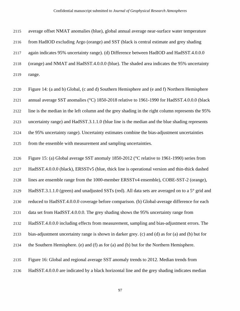
Confidential manuscript submitted to Journal of Geophysical Research Atmospheres
97
average offset NMAT anomalies (blue), global annual average near-surface water temperature 2115
from HadIOD excluding Argo (orange) and SST (black is central estimate and grey shading 2116
again indicates 95% uncertainty range). (d) Difference between HadIOD and HadSST.4.0.0.0 2117
(orange) and NMAT and HadSST.4.0.0.0 (blue). The shaded area indicates the 95% uncertainty 2118
range. 2119
Figure 14: (a and b) Global, (c and d) Southern Hemisphere and (e and f) Northern Hemisphere 2120
annual average SST anomalies (°C) 1850-2018 relative to 1961-1990 for HadSST.4.0.0.0 (black 2121
line is the median in the left column and the grey shading in the right column represents the 95% 2122
uncertainty range) and HadSST.3.1.1.0 (blue line is the median and the blue shading represents 2123
the 95% uncertainty range). Uncertainty estimates combine the bias-adjustment uncertainties 2124
from the ensemble with measurement and sampling uncertainties. 2125
Figure 15: (a) Global average SST anomaly 1850-2012 (°C relative to 1961-1990) series from 2126
HadSST.4.0.0.0 (black), ERSSTv5 (blue, thick line is operational version and thin-thick dashed 2127
lines are ensemble range from the 1000-member ERSSTv4 ensemble), COBE-SST-2 (orange), 2128
HadSST.3.1.1.0 (green) and unadjusted SSTs (red). All data sets are averaged on to a 5° grid and 2129
reduced to HadSST.4.0.0.0 coverage before comparison. (b) Global-average difference for each 2130
data set from HadSST.4.0.0.0. The grey shading shows the 95% uncertainty range from 2131
HadSST.4.0.0.0 including effects from measurement, sampling and bias-adjustment errors. The 2132
bias-adjustment uncertainty range is shown in darker grey. (c) and (d) as for (a) and (b) but for 2133
the Southern Hemisphere. (e) and (f) as for (a) and (b) but for the Northern Hemisphere. 2134
Figure 16: Global and regional average SST anomaly trends to 2012. Median trends from 2135
HadSST.4.0.0.0 are indicated by a black horizontal line and the grey shading indicates median 2136

Confidential manuscript submitted to Journal of Geophysical Research Atmospheres
98
and 95% uncertainty range including effects from measurement, sampling and bias-adjustment 2137
errors. The bias-adjustment uncertainty range is shown in darker grey; ERSSTv5 (blue), the 2138
lozenge is the operational version and the vertical line is the 95% ensemble range from the 1000-2139
member ERSSTv4 ensemble); COBE-SST-2 (orange); HadSST.3.1.1.0 (green); and unadjusted 2140
SSTs (red). 2141
Figure 17: (a) Standard deviation of SST anomalies (°C), (b) Zonal length scale Lx (km) and (c) 2142
meridional length scale Ly (km) used in the interpolation scheme.. 2143
2144
Figure 18: Example of the inputs and outputs of the interpolation for July 2003. (a) gridded SST 2145
anomalies (°C) from ships. (b) gridded SST anomalies from buoys. (c) interpolated SST 2146
anomalies. (d) estimated ERI biases (°C). Note that the ERI data are a subset of the ship data so 2147
the coverage is not identical. 2148
Figure 19: Tests of effectiveness of the reconstruction method from 2000-2014. Blue lines show 2149
results for the 19th century coverage tests, red lines show the results of the missing-at-random 2150
tests and the purple lines show the test where data were removed at selected locations of Argo 2151
observations. (a) probability distribution for chi-squared statistics calculated from the withheld 2152
data. (b) average of histograms from all scaled, withheld observations in the 19th century 2153
coverage test (blue line) compared to the samples drawn from the posterior of the reconstruction 2154
(black line and grey shading). (c) as for (b) but for the missing-at-random test (red). (d) as for (b) 2155
but for the test where data were removed at the locations of Argo observations (purple). In (d) 2156
the dashed purple line shows the offset that occurs when doing the reconstruction based on 2157
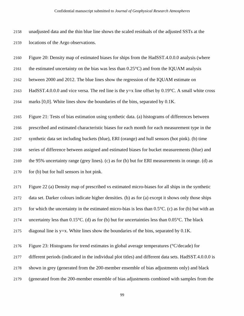
Confidential manuscript submitted to Journal of Geophysical Research Atmospheres
99
unadjusted data and the thin blue line shows the scaled residuals of the adjusted SSTs at the 2158
locations of the Argo observations. 2159
Figure 20: Density map of estimated biases for ships from the HadSST.4.0.0.0 analysis (where 2160
the estimated uncertainty on the bias was less than 0.25°C) and from the IQUAM analysis 2161
between 2000 and 2012. The blue lines show the regression of the IQUAM estimate on 2162
HadSST.4.0.0.0 and vice versa. The red line is the y=x line offset by 0.19°C. A small white cross 2163
marks [0,0]. White lines show the boundaries of the bins, separated by 0.1K. 2164
Figure 21: Tests of bias estimation using synthetic data. (a) histograms of differences between 2165
prescribed and estimated characteristic biases for each month for each measurement type in the 2166
synthetic data set including buckets (blue), ERI (orange) and hull sensors (hot pink). (b) time 2167
series of difference between assigned and estimated biases for bucket measurements (blue) and 2168
the 95% uncertainty range (grey lines). (c) as for (b) but for ERI measurements in orange. (d) as 2169
for (b) but for hull sensors in hot pink. 2170
Figure 22 (a) Density map of prescribed vs estimated micro-biases for all ships in the synthetic 2171
data set. Darker colours indicate higher densities. (b) as for (a) except it shows only those ships 2172
for which the uncertainty in the estimated micro-bias is less than 0.5°C. (c) as for (b) but with an 2173
uncertainty less than 0.15°C. (d) as for (b) but for uncertainties less than 0.05°C. The black 2174
diagonal line is y=x. White lines show the boundaries of the bins, separated by 0.1K. 2175
Figure 23: Histograms for trend estimates in global average temperatures (°C/decade) for 2176
different periods (indicated in the individual plot titles) and different data sets. HadSST.4.0.0.0 is 2177
shown in grey (generated from the 200-member ensemble of bias adjustments only) and black 2178
(generated from the 200-member ensemble of bias adjustments combined with samples from the 2179
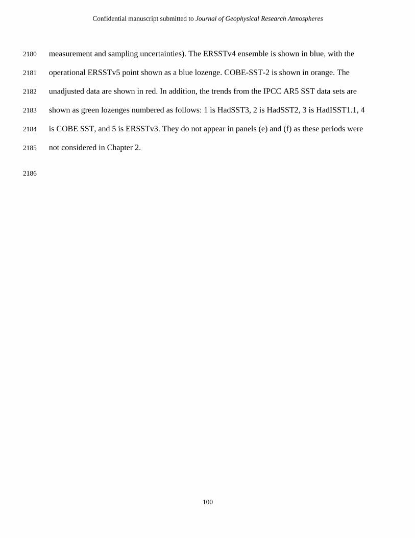
Confidential manuscript submitted to Journal of Geophysical Research Atmospheres
100
measurement and sampling uncertainties). The ERSSTv4 ensemble is shown in blue, with the 2180
operational ERSSTv5 point shown as a blue lozenge. COBE-SST-2 is shown in orange. The 2181
unadjusted data are shown in red. In addition, the trends from the IPCC AR5 SST data sets are 2182
shown as green lozenges numbered as follows: 1 is HadSST3, 2 is HadSST2, 3 is HadISST1.1, 4 2183
is COBE SST, and 5 is ERSSTv3. They do not appear in panels (e) and (f) as these periods were 2184
not considered in Chapter 2. 2185
2186

Figure 1.

1850 1855 1860 1865 1870 1875 18800
2
4
6
8
10
12
141k
obs
erva
tions
/mon
th(a) 1850-1880, Number of obs.
1850 1855 1860 1865 1870 1875 18800
2
4
6
8
1k s
uper
obs
erva
tions
/mon
th (b) 1850-1880, Superobservations
1880 1900 1920 1940 1960 1980 20000
100
200
300
400
500
1k o
bser
vatio
ns/m
onth Globe
Southern HemisphereNorthern Hemisphere
(c) 1880-2000, Number of obs.
1880 1900 1920 1940 1960 1980 20000
20
40
60
80
1k s
uper
obs
erva
tions
/mon
th (d) 1880-2000, Superobservations
2000 2005 2010 20150
500
1000
1500
2000
1k o
bser
vatio
ns/m
onth
(e) 2000-2018, Number of obs.
2000 2005 2010 20150
10
20
30
40
50
60
1k s
uper
obs
erva
tions
/mon
th (f) 2000-2018, Superobservations
Date produced: Mon Mar 18 09:28:44 GMT 2019. From code revision:838

Figure 2.

1920 1940 1960 1980 2000
0.0
0.2
0.4
0.6
0.8
1.0W
eig
ht
in g
lob
al a
ve
rag
e(a) Globe Unknown
Buckets
ERI
Hull
Drifters
Moorings
1920 1940 1960 1980 2000
0.0
0.2
0.4
0.6
0.8
1.0
We
igh
t in
glo
ba
l a
ve
rag
e
(b) SH
1920 1940 1960 1980 2000
0.0
0.2
0.4
0.6
0.8
1.0
We
igh
t in
glo
ba
l a
ve
rag
e
(c) NH
Date produced: Mon Mar 18 09:31:37 GMT 2019. From code revision:838

Figure 3.

90E 180 90W 0
90S
45S
0
45N
90N
-5 -1.6 -0.8 0 0.8 1.6 5
(a) SST anomalies, June 2003
90E 180 90W 0
90S
45S
0
45N
90N
0 1 10 100 1000 1e+4
(b) Number of Observations
90E 180 90W 0
90S
45S
0
45N
90N
0 20 40 60 80 100
(c) Number of Super Observations
90E 180 90W 0
90S
45S
0
45N
90N
0 0.2 0.4 0.6 0.8 1
(d) Fraction of ERI
90E 180 90W 0
90S
45S
0
45N
90N
0 0.2 0.4 0.6 0.8 1
(e) Fraction of Drifters
90E 180 90W 0
90S
45S
0
45N
90N
0 0.2 0.4 0.6 0.8 1
(f) Fraction of Moorings
90E 180 90W 0
90S
45S
0
45N
90N
0 0.2 0.4 0.6 0.8 2
(g) Uncorrelated error uncertainty
90E 180 90W 0
90S
45S
0
45N
90N
0 0.2 0.4 0.6 0.8 2
(h) Sampling error uncertainty
90E 180 90W 0
90S
45S
0
45N
90N
0 0.2 0.4 0.6 0.8 2
(i) Microbias error uncertainty

Figure 4.

SR02 R06 HadIOD ICOADSSection 4.1.1Generate set of bucket corrections by blending R06 and SR02 style corrections Section 4.1.2Estimate biases for subsets of ICOADS data using sub-surface profile dataSection 4.1.4Generate constrained ensemble of start and end dates for bucket transitions and estimate fraction of correct metadata. Gridder - Section 3Subset dataFinal AdjustmentsBased on generated biases and parameters, bias adjust the whole data set..correct start andend datesHadSST.4.0.0.0

Figure 5.

1860 1880 1900 1920 1940
-0.5
-0.4
-0.3
-0.2
-0.1
0.0
0.1
0.2C
orr
ection (
oC
)(a) R06 style corrections
1860 1880 1900 1920 1940
-0.5
-0.4
-0.3
-0.2
-0.1
0.0
0.1
0.2
Corr
ection (
oC
)
(b) SR02 style corrections
1860 1880 1900 1920 1940
-0.5
-0.4
-0.3
-0.2
-0.1
0.0
0.1
0.2
Corr
ection (
oC
)
(c) combined R06 and SR02 corrections
Jan Mar May Jul Sep Nov
-0.5
-0.4
-0.3
-0.2
-0.1
0.0
0.1
0.2
Bia
s (
oC
)
(d) Insulated bucket bias, Btr

Figure 6.
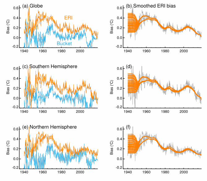
1940 1960 1980 2000
-0.2
0.0
0.2
0.4
0.6B
ias (
oC
)(a) Globe
ERI
Bucket
1940 1960 1980 2000
-0.2
0.0
0.2
0.4
0.6
Bia
s (
oC
)
(b) Smoothed ERI bias
1940 1960 1980 2000
-0.2
0.0
0.2
0.4
0.6
Bia
s (
oC
)
(c) Southern Hemisphere
1940 1960 1980 2000
-0.2
0.0
0.2
0.4
0.6
Bia
s (
oC
)
(d)
1940 1960 1980 2000
-0.2
0.0
0.2
0.4
0.6
Bia
s (
oC
)
(e) Northern Hemisphere
1940 1960 1980 2000
-0.2
0.0
0.2
0.4
0.6
Bia
s (
oC
)
(f)

Figure 7.

1940 1960 1980 2000
0.0
0.5
1.0
1.5
Estim
ate
d f
ractio
n c
orr
ectly la
be
lled (a) Rejected series of fcorrect
1940 1960 1980 2000
0.0
0.5
1.0
1.5
Estim
ate
d f
ractio
n c
orr
ectly la
be
lled (b) Accepted series of fcorrect
1930 1935 1940 1945 1950 1955 1960Start date of transition
1930
1940
1950
1960
1970
1980
En
d d
ate
of
tra
nsitio
n
(c) Rejected/accepted start and end dates
1940 1960 1980 2000
0.0
0.5
1.0
1.5
Fra
ctio
n o
f co
rre
ct
bu
cke
t a
ssig
nm
en
ts (d) Summary

Figure 8.

Bia
s (
oC
)
-0.6
-0.4
-0.2
-0.0
0.2
0.4(a) Globe, bias
Bia
s (
oC
)
-0.6
-0.4
-0.2
-0.0
0.2
0.4(b) Globe, bias relative to 1961-1990
Bia
s (
oC
)
-0.6
-0.4
-0.2
-0.0
0.2
0.4(c) Southern Hemisphere, bias
Bia
s (
oC
)
-0.6
-0.4
-0.2
-0.0
0.2
0.4(d) Southern Hemisphere, bias relative to 1961-1990
Bia
s (
oC
)
-0.6
-0.4
-0.2
-0.0
0.2
0.4(e) Northern Hemisphere, bias
Bia
s (
oC
)
-0.6
-0.4
-0.2
-0.0
0.2
0.4
1860 1880 1900 1920 1940 1960 1980 2000
(f) Northern Hemisphere, bias relative to 1961-1990
Date produced: Mon Mar 18 09:29:42 GMT 2019. From code revision:838

Figure 9.

An
om
aly
(oC
)
-0.8
-0.6
-0.4
-0.2
-0.0
0.2
0.4
0.6 (a) Globe, anomaly wrt unadjusted 1961-1990 climatology
An
om
aly
(oC
)
(b) Globe, anomaly wrt adjusted 1961-1990 climatology
-0.8
-0.6
-0.4
-0.2
-0.0
0.2
0.4
0.6
An
om
aly
(oC
)
-0.8
-0.6
-0.4
-0.2
-0.0
0.2
0.4
0.6 (c) Southern Hemisphere, anomaly wrt unadjusted 1961-1990 climatology
An
om
aly
(oC
)
(d) Southern Hemisphere, anomaly wrt adjusted 1961-1990 climatology
-0.8
-0.6
-0.4
-0.2
-0.0
0.2
0.4
0.6
An
om
aly
(oC
)
-0.8
-0.6
-0.4
-0.2
-0.0
0.2
0.4
0.6 (e) Northern Hemisphere, anomaly wrt unadjusted 1961-1990 climatology
An
om
aly
(oC
)
(f) Northern Hemisphere, anomaly wrt adjusted 1961-1990 climatology
-0.8
-0.6
-0.4
-0.2
-0.0
0.2
0.4
0.6
1860 1880 1900 1920 1940 1960 1980 2000
Date produced: Mon Mar 18 09:29:42 GMT 2019. From code revision:838

Figure 10.

1940 1960 1980 2000Year
-0.5
0.0
0.5
An
om
aly
(oC
)(a) Globe unadjusted
ERI
Bucket
1940 1960 1980 2000Year
-0.5
0.0
0.5
An
om
aly
(oC
)
(b) Globe adjusted
1940 1960 1980 2000Year
-1.0
-0.5
0.0
0.5
1.0
An
om
aly
(oC
)
(c) Southern Hemisphere unadjusted
1940 1960 1980 2000Year
-1.0
-0.5
0.0
0.5
1.0
An
om
aly
(oC
)
(d) Southern Hemisphere adjusted
1940 1960 1980 2000Year
-0.5
0.0
0.5
1.0
An
om
aly
(oC
)
(e) Northern Hemisphere unadjusted
1940 1960 1980 2000Year
-0.5
0.0
0.5
1.0
An
om
aly
(oC
)
(f) Northern Hemisphere adjusted
Date produced: Mon Mar 18 11:19:08 GMT 2019. From code revision:838

Figure 11.

-0.2
0.0
0.2
0.4
0.6
Anom
aly
(oC
)
(a) Argo
(b)
-0.2
0.0
0.2
0.4
0.6
Anom
aly
(oC
)
(c) ARC
(d)
-0.2
0.0
0.2
0.4
0.6
An
om
aly
(oC
)
(e) Buoys
1990 1995 2000 2005 2010 2015
(f)
Date produced: Mon Mar 18 09:43:11 GMT 2019. From code revision:838

Figure 12.
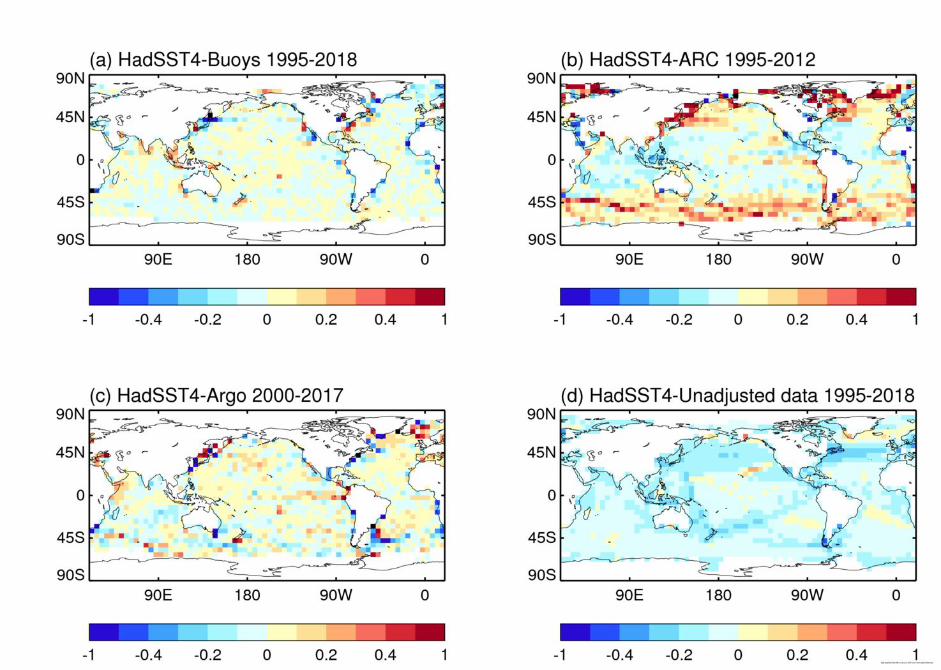

Figure 13.

1900 1920 1940 1960 1980 2000
-0.8
-0.6
-0.4
-0.2
0.0
0.2
0.40.6
Anom
aly
(oC
)(a) HadNMAT.2.0.1.0 and HadSST.4.0.0.0
1900 1920 1940 1960 1980 2000
-0.4
-0.2
0.0
0.2
0.4
Diffe
rence (
oC
)
(b) HadNMAT.2.0.1.0 minus HadSST.4.0.0.0
1900 1920 1940 1960 1980 2000
-0.8
-0.6
-0.4
-0.2
0.0
0.2
0.40.6
Anom
aly
(oC
)
(c) HadIOD, HadNMAT.2.0.1.0 and HadSST.4.0.0.0
1900 1920 1940 1960 1980 2000
-0.4
-0.2
0.0
0.2
0.4
An
om
aly
(oC
)
(d) HadIOD, HadNMAT.2.0.1.0 minus HadSST.4.0.0.0
Date produced: Mon Mar 18 10:22:23 GMT 2019. From code revision:838

Figure 14.
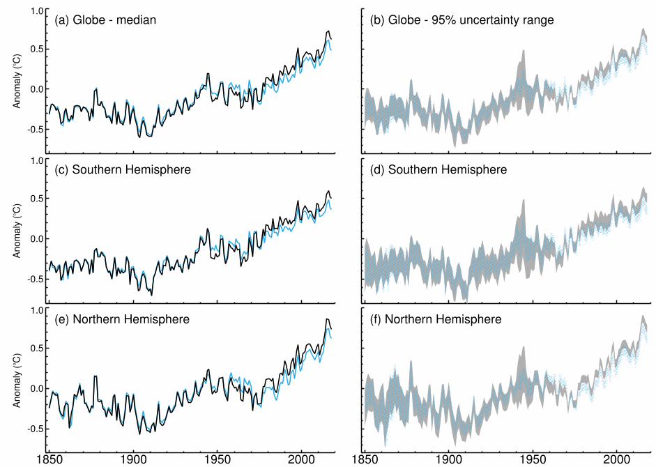
-0.5
0.0
0.5
1.0A
no
ma
ly (
oC
)(a) Globe - median
(b) Globe - 95% uncertainty range
-0.5
0.0
0.5
1.0
An
om
aly
(oC
)
(c) Southern Hemisphere
(d) Southern Hemisphere
-0.5
0.0
0.5
1.0
An
om
aly
(oC
)
(e) Northern Hemisphere
1850 1900 1950 2000
(f) Northern Hemisphere
1850 1900 1950 2000

Figure 15.

-1.0
-0.8
-0.6
-0.4
-0.2
-0.0
0.2
0.4
0.6
0.8 (a) Globe
-0.2-0.1 0.0 0.1 0.2
(b) difference
-1.0
-0.8
-0.6
-0.4
-0.2
-0.0
0.2
0.4
0.6
0.8 (c) Southern Hemisphere
-0.2-0.1 0.0 0.1 0.2
(d) difference
-1.0
-0.8
-0.6
-0.4
-0.2
-0.0
0.2
0.4
0.6
0.8 (e) Northern Hemisphere
-0.2-0.1 0.0 0.1 0.2
(f) difference
1900 1920 1940 1960 1980 2000
An
om
aly
(oC
) re
lative
to
19
61
-19
90
Date produced: Mon Mar 18 11:14:35 GMT 2019. From code revision:838

Figure 16.

-0.1
0.0
0.1
0.2
Tre
nd (
o C/d
ecad
e)
1900
1910
1920
1930
1940
1950
1960
1970
1980
1990
2000
(a) Globe
-0.1
0.0
0.1
0.2
Tre
nd (
o C/d
ecad
e)
1900
1910
1920
1930
1940
1950
1960
1970
1980
1990
2000(b) Southern Hemisphere
-0.1
0.0
0.1
0.2
Tre
nd (
o C/d
ecad
e)
1900
1910
1920
1930
1940
1950
1960
1970
1980
1990
2000(c) Northern Hemisphere
-0.1
0.0
0.1
0.2
0.3
0.4T
rend
(o C
/dec
ade)
1900
1910
1920
1930
1940
1950
1960
1970
1980
1990
2000
(d) North Atlantic
Date produced: Mon Mar 18 11:15:08 GMT 2019. From code revision:838

Figure 17.

90E 180 90W 0
90S
45S
0
45N
90N
0 0.4 0.8 1.2 1.6 2
(a) Standard Deviation
90E 180 90W 0
90S
45S
0
45N
90N
0 4000 8000 1.2e+4 1.6e+4 2e+4
(b) Zonal length scale
90E 180 90W 0
90S
45S
0
45N
90N
0 4000 8000 1.2e+4 1.6e+4 2e+4
(c) Meridional length scale
Date produced: Mon Mar 18 09:26:53 GMT 2019. From code revision:838

Figure 18.

90E 180 90W 0
90S
45S
0
45N
90N
-5 -1.6 -0.8 0 0.8 1.6 5
(a) Ship anomalies July 2003
90E 180 90W 0
90S
45S
0
45N
90N
-5 -1.6 -0.8 0 0.8 1.6 5
(b) Buoy anomalies July 2003
90E 180 90W 0
90S
45S
0
45N
90N
-5 -1.6 -0.8 0 0.8 1.6 5
(c) Analysed anomalies July 2003
90E 180 90W 0
90S
45S
0
45N
90N
-5 -1.6 -0.8 0 0.8 1.6 5
(d) ERI Bias July 2003
Date produced: Mon Mar 18 09:26:55 GMT 2019. From code revision:838

Figure 19.
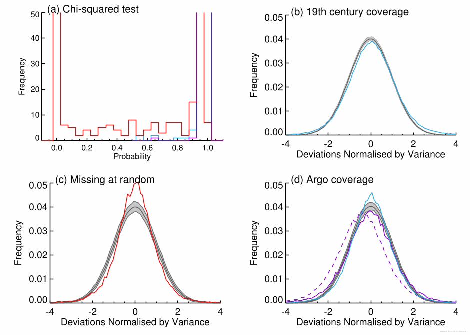
0.0 0.2 0.4 0.6 0.8 1.0Probability
0
10
20
30
40
50F
requency
(a) Chi-squared test
-4 -2 0 2 4Deviations Normalised by Variance
0.00
0.01
0.02
0.03
0.04
0.05
Fre
qu
en
cy
(b) 19th century coverage
-4 -2 0 2 4Deviations Normalised by Variance
0.00
0.01
0.02
0.03
0.04
0.05
Fre
qu
en
cy
(c) Missing at random
-4 -2 0 2 4Deviations Normalised by Variance
0.00
0.01
0.02
0.03
0.04
0.05
Fre
qu
en
cy
(d) Argo coverage
Date produced: Mon Mar 18 09:27:16 GMT 2019. From code revision:838

Figure 20.

-3 -2 -1 0 1 2 3IQUAM bias estimate (oC)
-3
-2
-1
0
1
2
3H
adS
ST
.4.0
.0.0
bia
s e
stim
ate
(oC
)

Figure 21.

-0.4 -0.2 0.0 0.2 0.40.00
0.05
0.10
0.15
0.20P
roba
bilit
y
BucketERIHull Sensors
(a)
1995 2000 2005 2010 2015-0.4
-0.2
0.0
0.2
0.4
Est
imat
ed-T
rue
bias
(o C) (b) Bucket
1995 2000 2005 2010 2015-0.4
-0.2
0.0
0.2
0.4
Est
imat
ed-T
rue
bias
(o C) (c) ERI
1995 2000 2005 2010 2015-0.4
-0.2
0.0
0.2
0.4
Est
imat
ed-T
rue
bias
(o C) (d) Hull sensors

Figure 22.

-2 -1 0 1 2True bias (oC)
-2
-1
0
1
2E
stim
ate
d b
ias (
oC
)(a) All
-2 -1 0 1 2True bias (oC)
-2
-1
0
1
2
Estim
ate
d b
ias (
oC
)
(b) Uncertainty < 0.5oC
-2 -1 0 1 2True bias (oC)
-2
-1
0
1
2
Estim
ate
d b
ias (
oC
)
(c) Uncertainty < 0.15oC
-2 -1 0 1 2True bias (oC)
-2
-1
0
1
2
Estim
ate
d b
ias (
oC
)
(d) Uncertainty < 0.05oC

Figure 23.

0.02 0.04 0.06 0.08 0.10Trend (oC/decade)
0.00
0.02
0.04
0.06
0.08
0.10
0.12
0.14P
robabili
ty(a) Globe Trends 1880-2012
ERSSTv4
HadSST.4.0.0.0
HadSST.4.0.0.0(ensemble only)
Unadjusted
123 5
0.04 0.06 0.08 0.10 0.12Trend (oC/decade)
0.00
0.02
0.04
0.06
0.08
0.10
Pro
babili
ty
(b) Trends 1901-2012
1 23 4 5
0.06 0.08 0.10 0.12Trend (oC/decade)
0.00
0.05
0.10
0.15
Pro
babili
ty
(c) Trends 1951-2012
1 23 4 5
0.06 0.08 0.10 0.12 0.14Trend (oC/decade)
0.00
0.05
0.10
0.15
0.20
Pro
babili
ty
(d) Trends 1979-2012
COBE-SST-2
1234 5
-0.02 0.00 0.02 0.04 0.06 0.08Trend (oC/decade)
0.00
0.05
0.10
0.15
0.20
0.25
Pro
ba
bili
ty
(e) Trends 1998-2012
-0.08 -0.06 -0.04 -0.02 0.00 0.02Trend (oC/decade)
0.00
0.02
0.04
0.06
0.08
0.10
0.12
0.14
Pro
ba
bili
ty
(f) Trends 2002-2012
Date produced: Mon Mar 18 09:28:34 GMT 2019. From code revision:838