
Rutgers-Camden Editorial Style Guide - Rutgers University-Camden
date post
20-Dec-2015Category
view
218download
0
1
Algorithms for Port of Entry Inspection for WMDs
Fred S. RobertsDyDAn CenterRutgers University

2
Port of Entry Inspection Algorithms
•Goal: Find ways to intercept illicit nuclear materials and weapons
destined for the U.S. via the maritime transportation system
•Currently inspecting only small % of containers arriving at ports
•Even inspecting 8% of containers in Port of NY/NJ might bring international trade to a halt (Larrabbee 2002)

3
Port of Entry Inspection Algorithms•Aim: Develop decision support algorithms that will help us to “optimally” intercept illicit materials and weapons subject to limits on delays, manpower, and equipment
•Find inspection schemes that minimize total “cost” including “cost” of false positives and false negatives
Mobile Vacis: truck-mounted gamma ray imaging system

4
Port of Entry Inspection Algorithms•My work on port of entry inspection has gotten me and our students and colleagues to some remarkable places.
Me on a Coast Guardboat in a tour of theharbor in Philadelphia

5

6
Sequential Decision Making Problem•Stream of containers arrives at a port•The Decision Maker’s Problem:
•Which to inspect?•Which inspections next based on previous results?
•Approach: –“decision logics”–combinatorial optimization methods–Builds on ideas of Stroud and Saeger at Los AlamosNational Laboratory–Need for new modelsand methods

7
Sequential Diagnosis Problem•Such sequential diagnosis problems arise in many areas:
–Communication networks (testing connectivity, paging cellular customers, sequencing tasks, …)–Manufacturing (testing machines, fault diagnosis, routing customer service calls, …)–Artificial intelligence/CS (optimal derivation strategies in knowledge bases, best-value satisficing search, coding decision trees, …)–Medicine (diagnosing patients, sequencing treatments, …)

8
Sequential Decision Making Problem•Containers arriving to be classified into categories.•Simple case: 0 = “ok”, 1 = “suspicious”
•Inspection scheme: specifies which inspections are to be made based on previous observations

9
Sequential Decision Making Problem
•Containers have attributes, each in a number of states
•Sample attributes:–Levels of certain kinds of chemicals or biological materials–Whether or not there are items of a certain kind in the cargo list–Whether cargo was picked up in a certain port

10
Sequential Decision Making Problem
•Currently used attributes:–Does ship’s manifest set off an “alarm”?–What is the neutron or Gamma emission count? Is it above threshold?–Does a radiograph image come up positive?–Does an induced fission test come up positive?
Gamma ray detector
11
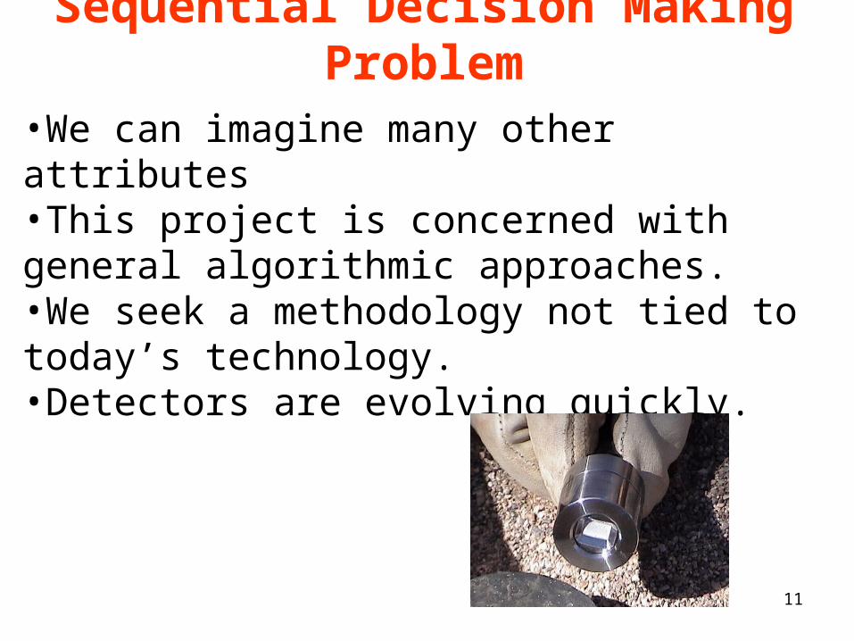
Sequential Decision Making Problem
•We can imagine many other attributes•This project is concerned with general algorithmic approaches.•We seek a methodology not tied to today’s technology.•Detectors are evolving quickly.

12
Sequential Decision Making Problem
•Simplest Case: Attributes are in state 0 or 1
•Then: Container is a binary string like 011001
•So: Classification is a decision function F that assigns each binary string to a category.
011001 F(011001)
If attributes 2, 3, and 6 are present, assign container to category F(011001).

13
Sequential Decision Making Problem
•If there are two categories, 0 and 1, decision function F is a Boolean function.
Example: F(000) = F(111) = 1, F(abc) = 0 otherwise
This classifies a container as positive iff it has none of the attributes or all of them.
1 =

14
Sequential Decision Making Problem
•Given a container, test its attributes until know enough to calculate the value of F.
•An inspection scheme tells us in which order to test the attributes to minimize cost.
•Even this simplified problem is hard computationally.

15
Sequential Decision Making Problem•This assumes F is known.•Simplifying assumption: Attributes are independent.•At any point we stop inspecting and output the value of F based on outcomes of inspections so far.•Complications: May be precedence relations in the components (e.g., can’t test attribute a4 before testing a6. •Or: cost may depend on attributes tested before.•F may depend on variables that cannot be directly tested or for which tests are too costly.

16
Sequential Decision Making Problem
•Such problems are hard computationally.•There are many possible Boolean functions F.•Even if F is fixed, problem of finding a good classification scheme (to be defined precisely below) is NP-complete. •Several classes of functions F allow for efficient inspection schemes:
–k-out-of-n systems–Certain series-parallel systems–Read-once systems–“regular” systems–Horn systems

17
Sensors and Inspection Lanes•n types of sensors measure presence or absence of the n attributes. •Many copies of each sensor.•Complication: different characteristics of sensors.•Entities come for inspection.•Which sensor of a given type to use?•Think of inspection lanes and queues.•Besides efficient inspection schemes, could decrease costs by:
–Buying more sensors–Change allocation of containers to sensor lanes.

18
Binary Decision Tree Approach•Sensors measure presence/absence of attributes.
•Binary Decision Tree: –Nodes are sensors or categories (0 or 1)–Two arcs exit from each sensor node, labeled left and right.–Take the right arc when sensor says the attribute is present, left arc otherwise

19
Binary Decision Tree Approach
•Reach category 1 from the root only through the path a0 to a1 to 1.
•Container is classified in category 1 iff it has both attributes a0 and a1 .
•Corresponding Boolean function F(11) = 1, F(10) = F(01) = F(00) = 0.
Figure 1

20
Binary Decision Tree Approach•Reach category 1 from the root by:a0 L to a1 R a2 R 1 ora0 R a2 R1
•Container classified in category 1 iff it hasa1 and a2 and not a0 or a0 and a2 and possibly a1.
•Corresponding Boolean function F(111) = F(101) = F(011) = 1, F(abc) = 0 otherwise.
Figure 2
21
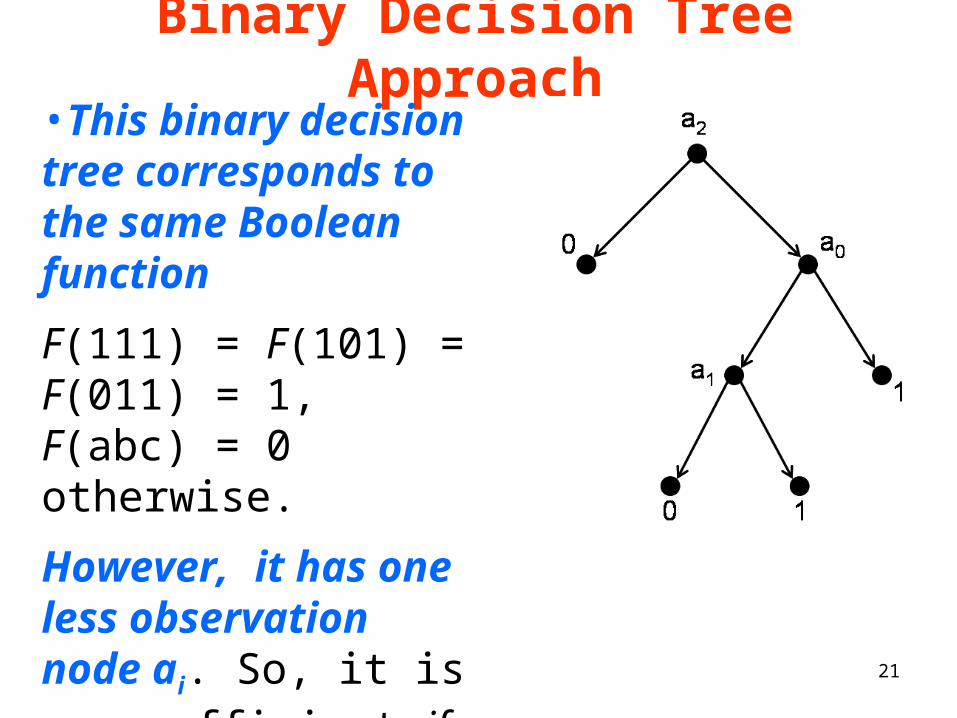
Binary Decision Tree Approach•This binary decision tree corresponds to the same Boolean function
F(111) = F(101) = F(011) = 1, F(abc) = 0 otherwise.
However, it has one less observation node ai. So, it is more efficient if all observations are equally costly and equally likely.
Figure 3

22
Binary Decision Tree Approach•Even if the Boolean function F is fixed, the problem of finding the “optimal” binary decision tree for it is very hard (NP-complete) if optimal means smallest number of sensor nodes.
•For small n = number of attributes, can try to solve it by brute force enumeration.
•Even for n = 4, not practical. (n = 4 at Port of Long Beach-Los Angeles)
Port of Long Beach

23
Binary Decision Tree ApproachPromising Approaches:
•Heuristic algorithms, approximations to optimal.•Special assumptions about the Boolean function F. •For “monotone” Boolean functions, integer programming formulations give promising heuristics.•Stroud and Saeger enumerate all “complete,” monotone Boolean functions and calculate the least expensive corresponding binary decision trees.•Their method practical for n up to 4, not n = 5.

24
Binary Decision Tree ApproachMonotone Boolean Functions:
•Given two strings x1x2…xn, y1y2…yn
•Suppose that xi yi for all i implies that F(x1x2…xn) F(y1y2…yn).•Then we say that F is monotone. •Then 11…1 has highest probability of being in category 1.
25
Binary Decision Tree Approach
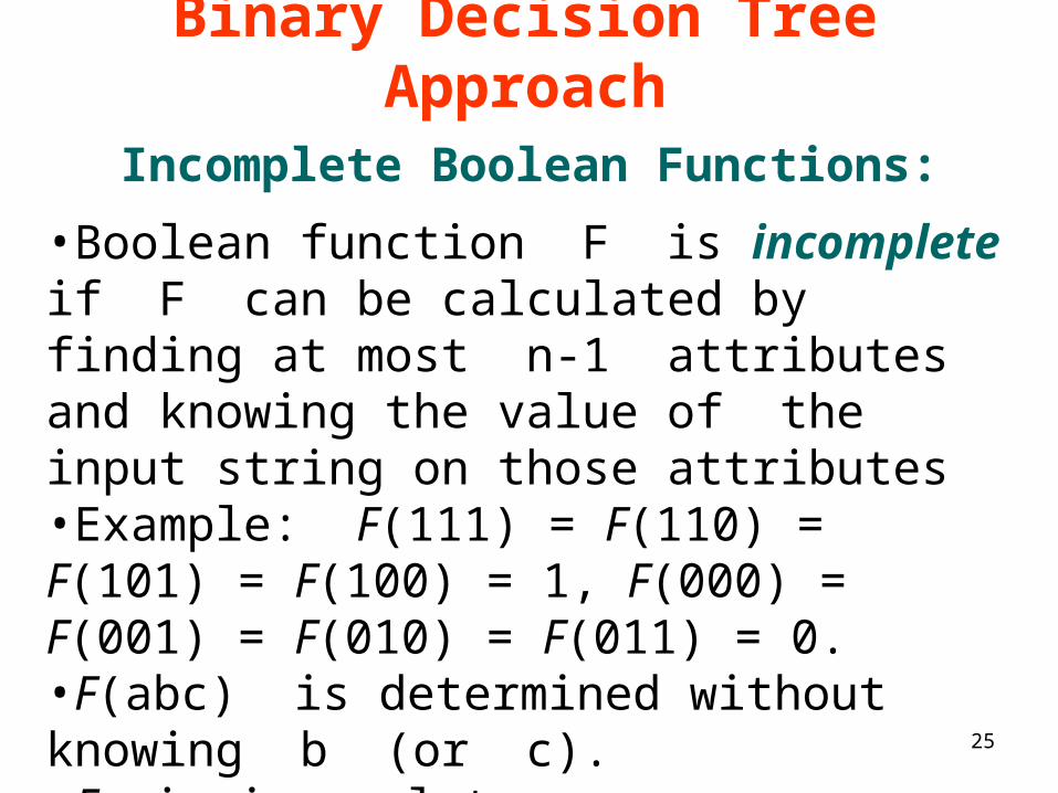
Incomplete Boolean Functions:
•Boolean function F is incomplete if F can be calculated by finding at most n-1 attributes and knowing the value of the input string on those attributes•Example: F(111) = F(110) = F(101) = F(100) = 1, F(000) = F(001) = F(010) = F(011) = 0. •F(abc) is determined without knowing b (or c).•F is incomplete.

26
Binary Decision Tree Approach
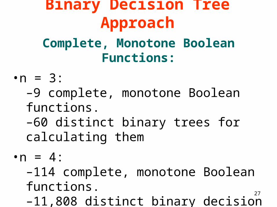
Complete, Monotone Boolean Functions:
•Stroud and Saeger: algorithm for enumerating binary decision trees implementing complete, monotone Boolean functions. •Feasible to implement up to n = 4.•n = 2:
–There are 6 monotone Boolean functions.–Only 2 of them are complete, monotone–There are 4 binary decision trees for calculating these 2 complete, monotone Boolean functions.
27
Binary Decision Tree Approach
Complete, Monotone Boolean Functions:
•n = 3:–9 complete, monotone Boolean functions.–60 distinct binary trees for calculating them
•n = 4:–114 complete, monotone Boolean functions.–11,808 distinct binary decision trees for calculating them.–(Compare 1,079,779,602 BDTs for all Boolean functions)

28
Binary Decision Tree Approach
Complete, Monotone Boolean Functions:
•n = 5:–6894 complete, monotone Boolean functions–263,515,920 corresponding binary decision trees.
•Combinatorial explosion! •Need alternative approaches; enumeration not feasible!•(Even worse: compare 5 x 10¹⁸ BDTs corresponding to all Boolean functions)

29
Cost Functions
•Stroud-Saeger method applies to more sophisticated cost models, not just cost = number of sensors in the BDT.•Using a sensor has a cost:
–Unit cost of inspecting one item with it–Fixed cost of purchasing and deploying it–Delay cost from queuing up at the sensor station
•Preliminary problem: disregard fixed and delay costs. Minimize unit costs.

30
Cost Functions
•Simplification so far: Disregard characteristics of population of entities being inspected. •Only count number of observation (attribute) nodes in the tree.
•Unit Cost Complication: How many nodes of the decision tree are actually visited during average container’s inspection? Depends on “distribution” of containers. In our early models, depends on probability of sensor errors and probability of bomb in a container.
31
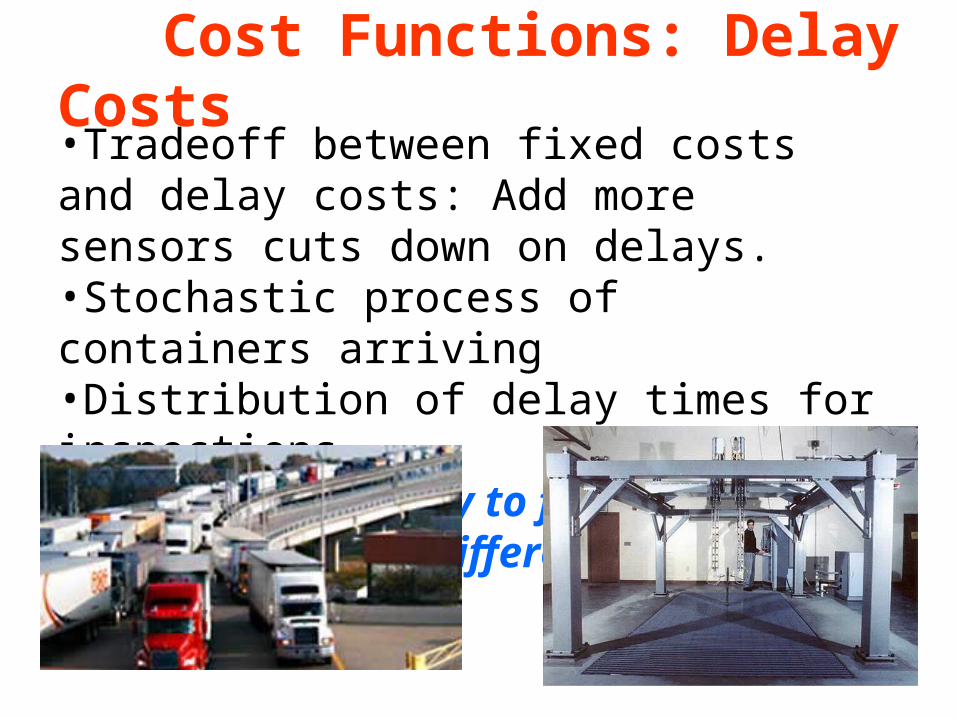
Cost Functions: Delay Costs•Tradeoff between fixed costs and delay costs: Add more sensors cuts down on delays.•Stochastic process of containers arriving•Distribution of delay times for inspections•Use queuing theory to find average delay times under different models

32
Cost Functions:Unit Costs
Tree Utilization•Complication: Assume cost depends on how many nodes of BDT are actually visited during an “average” container’s inspection. (This is sum of unit costs.)•Depends on characteristics of population of entities being inspected. •I.e., depends on “distribution” of containers. •In our early models, we assume we are given probability of sensor errors and probability of bomb in a container.•This allows us to calculate “expected” cost of utilization of the tree Cutil.

33
Cost Function used for Evaluating the Decision Trees.
Later: Expect to analyze models for distribution of attributes of containers and more sophisticated analysis of expected cost of utilizing the tree, bringing in delay costs.

34
Cost Functions
•Cost of false positive: Cost of additional tests.
–If it means opening the container, it’s very expensive.
•Cost of false negative: –Complex issue.–What is cost of a bomb going off in Manhattan?

35
Cost Functions: Sensor Errors•One Approach to False Positives/Negatives:Assume there can be Sensor Errors•Simplest model: assume that all sensors checking for attribute ai have same fixed probability of saying ai is 0 if in fact it is 1, and similarly saying it is 1 if in fact it is 0.•More sophisticated analysis later describes a model for determining probabilities of sensor errors. •Notation: X = state of nature (bomb or no bomb)
Y = outcome (of sensor or entire inspection process).

36
Probability of Error for The Entire TreeState of nature is zero (X = 0), absence of a bomb State of nature is one (X = 1), presence
of a bomb
Probability of false positive (P(Y=1|X=0))
for this tree is given by
Probability of false negative(P(Y=0|X=1))
for this tree is given by
A
B
C
0
1
0 1
A
B
C
0
1
0 1
P(Y=1|X=0) = P(YA=1|X=0) * P(YB=1|X=0) + P(YA=1|X=0) *P(YB=0|X=0)* P(YC=1|X=0)
Pfalsepositive
P(Y=0|X=1) = P(YA=0|X=1) + P(YA=1|X=1) *P(YB=0|X=1)*P(YC=0|X=1)
Pfalsenegative

37
Cost Function used for Evaluating the Decision Trees.
CTot = CFalsePositive *PFalsePositive + CFalseNegative *PFalseNegative + Cutil
CFalsePositive is the cost of false positive (Type I error)CFalseNegative is the cost of false negative (Type II error)PFalsePositive is the probability of a false positive occurringPFalseNegative is the probability of a false negative occurringCutil is the expected cost of utilization of the tree.
38
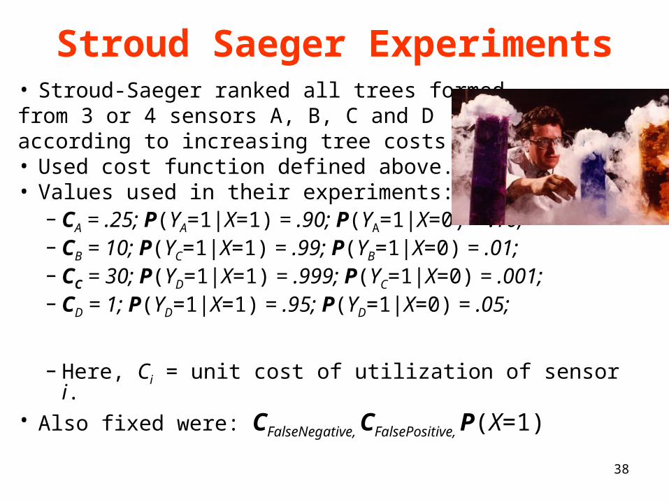
Stroud Saeger Experiments• Stroud-Saeger ranked all trees formedfrom 3 or 4 sensors A, B, C and D according to increasing tree costs. • Used cost function defined above. • Values used in their experiments:
– CA = .25; P(YA=1|X=1) = .90; P(YA=1|X=0) = .10;– CB = 10; P(YC=1|X=1) = .99; P(YB=1|X=0) = .01;– CC = 30; P(YD=1|X=1) = .999; P(YC=1|X=0) = .001;– CD = 1; P(YD=1|X=1) = .95; P(YD=1|X=0) = .05;
– Here, Ci = unit cost of utilization of sensor i. • Also fixed were: CFalseNegative, CFalsePositive, P(X=1)
39
Stroud Saeger Experiments: Our Sensitivity Analysis
• We have explored sensitivity of the Stroud-Saeger conclusions to variations in values of these three parameters.
• We estimated high and low values for these parameters and did experiments with selection of values from the interval of possible values.

40
Stroud Saeger Experiments: Our Sensitivity Analysis
– CFalseNegative was varied between 25 million and 10 billion dollars• Low and high estimates of direct and indirect costs
incurred due to a false negative.
– CFalsePositive was varied between $180 and $720
• Cost incurred due to false positive
(4 men * (3 -6 hrs) * (15 – 30 $/hr)– P(X=1) was varied between 1/10,000,000 and
1/100,000

41
Stroud Saeger Experiments: Our Sensitivity Analysis
n = 3 (use sensors A, B, C)• We chose one of the values from the interval of
values and then explored the highest ranked tree as the other two were chosen at random in the interval of values. 10,000 experiments for each fixed value.
• We looked for the variation in the top-ranked tree and how the top-rank related to choice of parameter values.
• Very surprising results.

42
Frequency of Top-ranked Trees when CFalseNegative and CFalsePositive are Varied
• 10,000 randomized experiments (randomly selected values of CFalseNegative and CFalsePositive from the specified range of values) for the median value of P(X=1).
• The above graph has frequency counts of the number of experiments when a particular tree was ranked first or second, or third and so on.
• Only three trees (7, 55 and 1) ever came first. 6 trees came second, 10 came third, 13 came fourth.
0 10 20 30 40 50 600
1000
2000
3000
4000
5000
6000
7000
Tree no.
Fre
qu
en
cy
1st2nd3rd4th5th
43
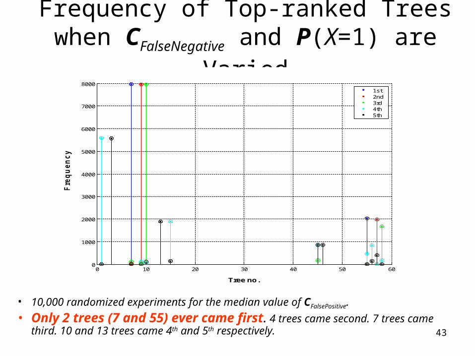
• 10,000 randomized experiments for the median value of CFalsePositive.
• Only 2 trees (7 and 55) ever came first. 4 trees came second. 7 trees came third. 10 and 13 trees came 4th and 5th respectively.
Frequency of Top-ranked Trees when CFalseNegative and P(X=1) are Varied
0 10 20 30 40 50 600
1000
2000
3000
4000
5000
6000
7000
8000
Tree no.
Fre
qu
en
cy
1st2nd3rd4th5th

44
• 10,000 randomized experiments for the median value of CFalseNegative. • Only 3 trees (7, 55 and 1) ever came first. 6 trees came second. 10
trees came third. 13 and 16 trees came 4th and 5th respectively.
Frequency of Top-ranked Trees when P(X=1) and CFalsePositive are Varied
0 10 20 30 40 50 600
1000
2000
3000
4000
5000
6000
7000
Fre
qu
en
cy
Tree no.
1st2nd3rd4th5th

45
Stroud Saeger Experiments: Our Sensitivity Analysis: 4 Sensors
• Second set of computer experiments: n = 4
(use sensors, A, B, C, D).
• Same values as before.
• Experiment 1: Fix values of two of CFalseNegative,
CFalsePositive, P(X=1) and vary the third through their interval of possible values.
• Experiment 2: Fix a value of one of CFalseNegative,
CFalsePositive, P(X=1) and vary the other two.
• Do 10,000 experiments each time.
• Look for the variation in the highest ranked tree.

46
Stroud Saeger Experiments: Our Sensitivity Analysis: 4 Sensors
• Experiment 1: Fix values of two of CFalseNegative, CFalsePositive, P(X=1) and vary the third.

47
CTot vs CFalseNegative for Ranked 1 Trees (Trees 11485(9651) and 10129(349))
Only two trees ever were ranked first, and one, tree 11485, was ranked first in 9651 out of 10,000 runs.

48
CTot vs CFalsePositive for Ranked 1 Trees (Tree no. 11485 (10000))
One tree, number 11485, was ranked first every time.

49
CTot vs P(X=1) for Ranked 1 Trees (Tree no. 11485(8372), 10129(488), 11521(1056))
Three trees dominated first place. Trees 10201(60), 10225(17) and 10153(7) also achieved first rank but with relatively low frequency.

50
Stroud Saeger Experiments: Our Sensitivity Analysis: 4 Sensors
• Experiment 2: Fix the values of one of CFalseNegative, CFalsePositive, P(X=1) and vary the others.

51
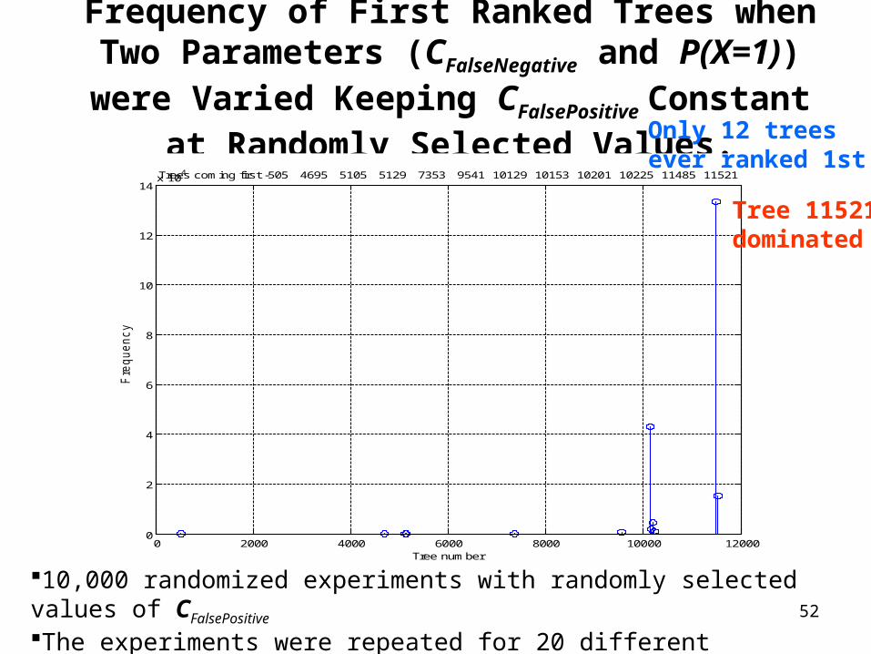
Frequency of First Ranked Trees when Two Parameters (CFalseNegative and CFalsePositive) were Varied Keeping P(X=1) Constant at Randomly Selected
Values.
0 2000 4000 6000 8000 10000 120000
0.2
0.4
0.6
0.8
1
1.2
1.4
1.6
1.8
2x 10
5 Trees coming first -9541 10129 10153 10201 11485 11521
Tree number
Fre
quency
10,000 randomized experiments with randomly selected values of P(X=1) The experiments were repeated for 20 different randomly selected values of P(X=1)
Only 6 treesever ranked 1st
Tree 11521dominated
52
Frequency of First Ranked Trees when Two Parameters (CFalseNegative and P(X=1)) were Varied
Keeping CFalsePositive Constant at Randomly Selected Values.
0 2000 4000 6000 8000 10000 120000
2
4
6
8
10
12
14x 10
4
Tree number
Fre
quency
Trees coming first -505 4695 5105 5129 7353 9541 10129 10153 10201 10225 11485 11521
10,000 randomized experiments with randomly selected values of CFalsePositive
The experiments were repeated for 20 different randomly selected values of CFalsePositive
Only 12 trees ever ranked 1st
Tree 11521dominated

53
Frequency of First Ranked Trees when Two Parameters (P(X=1) and CFalsePositive) were Varied
Keeping CFalseNegative Constant at Randomly Selected Values.
0.95 1 1.05 1.1 1.15 1.2
x 104
0
5
10
15x 10
4
Tree number
Fre
quency
Trees coming first -9541 10129 10153 10201 10225 11485 11521
10,000 randomized experiments with randomly selected values of CFalseNegative
The experiments were repeated for 20 different randomly selected values of CFalseNegative
Only 7 trees ever ranked1st
Tree 11521dominated

54
Conclusions from Sensitivity Analysis
• Considerable lack of sensitivity to modification in parameters for trees using 3 or 4 sensors.
• Very few optimal trees.
• Very few Boolean functions arise among optimal and near-optimal trees.

55
Modeling Sensor Errors•One Approach to Sensor Errors: Modeling Sensor Operation
•Threshold Model:–Sensors have different discriminating power–Many use counts (e.g., Gamma radiation counts)–See if count exceeds threshold–If so, say attribute is present.

56
Modeling Sensor Errors
Threshold Model:•Sensor i has discriminating power Ki, threshold Ti
•Attribute present if counts exceed Ti
•Seek threshold values that minimize the overall cost function, including costs of inspection, false positive/negative•Assume readings of category 0 containers follow a Gaussian distribution and similarly category 1 containers•Simulation approach
57
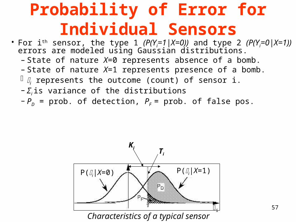
Probability of Error for Individual Sensors
• For ith sensor, the type 1 (P(Yi=1|X=0)) and type 2 (P(Yi=0|X=1)) errors are modeled using Gaussian distributions. – State of nature X=0 represents absence of a bomb.– State of nature X=1 represents presence of a bomb. i represents the outcome (count) of sensor i. – Σi is variance of the distributions– PD = prob. of detection, PF = prob. of false pos.
Ki
P(i|X=1)P(i|X=0)
Ti
Characteristics of a typical sensori
58
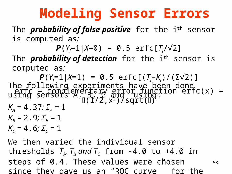
Modeling Sensor ErrorsThe probability of false positive for the ith sensor is computed as:
P(Yi=1|X=0) = 0.5 erfc[Ti/√2]The probability of detection for the ith sensor is computed as:
P(Yi=1|X=1) = 0.5 erfc[(Ti-Ki)/(Σ√2)]
erfc = complementary error function erfc(x) = (1/2,x2)/sqrt()
The following experiments have been done using sensors A, B, C and using:
KA = 4.37; ΣA = 1KB = 2.9; ΣB = 1KC = 4.6; ΣC = 1
We then varied the individual sensor thresholds TA, TB and TC from -4.0 to +4.0 in steps of 0.4. These values were chosen since they gave us an “ROC curve” for the individual sensors over a complete range P(Yi=1|X=0) and P(Yi=1|X=1)

59
Frequency of First Ranked Trees for Variations in Sensor Thresholds
• 68,921 experiments were conducted, as each Ti was varied through its entire range. (n = 3)• The above graph has frequency counts of the number of experiments when a particular tree
was ranked first. There are 15 such trees. Tree 37 had the highest frequency of attaining rank one.
0 10 20 30 40 50 600
2000
4000
6000
8000
10000
12000
14000
16000
18000
Tree no.
Fre
qu
en
cy

60
Modeling Sensor Errors•A number of trees ranking first in other experiments also ranked first here.
•Similar results in case of n = 4.•4,194,481 experiments.•244 different trees were ranked first in at least one experiment.•Trees ranked first in other experiments also frequently appeared first here.
•Conclusion: considerable insensitivity to change of threshold.

61
New Approaches to Optimum Threshold Computation
• Extensive search over a range of thresholds has some practical drawbacks:– Large number of threshold values for every sensor– Large step size– Grows exponentially with the number of sensors
(computationally infeasible for n > 4)
• A non-linear optimization approach proves more satisfactory:– A combination of Gradient Descent and modified
Newton’s methods

62
Optimum Threshold Computation• We implemented standard approaches including:
– Gradient Descent Method– Newton’s Method in Optimization
• In Gradient Descent Method we have to adjust the “step size” heuristically, while the Newton method uses the Hessian matrix to adjust the step size automatically
2 2 2
2
2 2 2
2
2 2 2
2
a a b a n
b a b b n
n a n b n
f f f
T T T T T
f f f
f T T T T T
f f f
T T T T T
H
Though the computation of the Hessian matrix is a little expensive and tedious, the method quickly converges in fewer iterations than the gradient descent method

63
Problems with Standard Approaches• Gradient Descent Method: Setting the value of the step
size heuristically, since:– Too small step size results in large number of iterations to
reach the minimum– Too big step size results in skipping the minimum
• Newton’s Method:– The convergence depends largely on the starting point.
This method occasionally drifts in the wrong direction and hence fails to converge.
• Solution: combination of gradient descent and Newton’s methods

64
A Combined Method• The Hessian matrix H f(τ) might not be a well-
conditioned, positive definite matrix
• We explored alternative approaches to computing positive definite approximations to H f(τ)– Modified Cholesky Algorithms
•If the Hessian matrix H f(τ) is ill-conditioned, we take small steps towards the minimum using the gradient descent method until it becomes well conditioned

65
Results: Threshold Optimization• Costs of false positive CFalsePositive and false negative
CFalseNegative and prior probability of occurrence of a bad container, P(X=1), were fixed as means of the min and max values given by Stroud and Saeger (same as we used in earlier experiments)
• We were able to converge to a (hopefully-close-to-minimum) cost every time with a modest number of iterations. For example:– For 3 sensors, it took an average of 0.081 seconds (as opposed to
0.387 seconds using extensive search) to converge to a cost for all 114 trees
– For 4 sensors, it took an average of 0.196 seconds (as opposed to more than 2 seconds using extensive search) to converge to a cost for all 66,936 trees
• In each case, min cost attained with new algorithm was lower, and often much lower, than that attained with extensive search.

66
Results: Threshold Optimization
Many times the minimum obtained using the optimization method was considerably less than the one from the extensive search technique.
0 20 40 60 80 100
100
150
200
250
300
350
400
450
500
Tree Number
Tot
al C
ost
Tree costs at optimum thresholds
Combined OptimizationExtensive search

67
New Idea: Searching through a Generalized Tree Space
• We expand the space of trees from those corresponding to Stroud and Saeger’s “Complete” and “Monotonic” Boolean Functions to “Complete and Monotonic BDTs”, because…
• Unlike Boolean functions, BDTs may not consider all sensor outputs to give a final decision
• Advantages:– Allow more potentially useful trees to participate in the analysis– Help define an irreducible tree space for search operations– Move focus from Boolean Functions to Binary Decision Trees

68
Revisiting Monotonicity• Monotonic Decision Trees
– A binary decision tree will be called monotonic if all the left leaves are class “0” and all the right leaves are class “1”.
• Example:a b c F(abc) 0 0 0 00 0 1 00 1 0 10 1 1 11 0 0 0 1 0 1 11 1 0 01 1 1 1
a b b
b c a c c a
0 1 0 1 0 c a 1 0 a 1 c
0 1 1 0 0 1 0 1 b c
c c b b
0 a a 1 0 a a 1
0 1 1 0 1 0 0 1
c c
a b b a
b 0 a 1 0 a b 1
0 1 0 1 1 0 0 1
All these trees correspond to same monotonic Boolean functionOnly one is a monotonic BDT.

69
Revisiting Completeness• Complete Decision Trees
– A binary decision tree will be called complete if every sensor occurs at least once in the tree and, at any non-leaf node in the tree, its left and right sub-trees are not identical.
• Example:a b c F(abc) 0 0 0 00 0 1 10 1 0 10 1 1 11 0 0 0 1 0 1 11 1 0 11 1 1 1
a
b c
c 1 b 1
0 1 0 1
a
c b
b 1 c 1
0 1 0 1
a
c c
b 1 b 1
0 1 0 1
a
b b
c 1 c 1
0 1 0 1
70
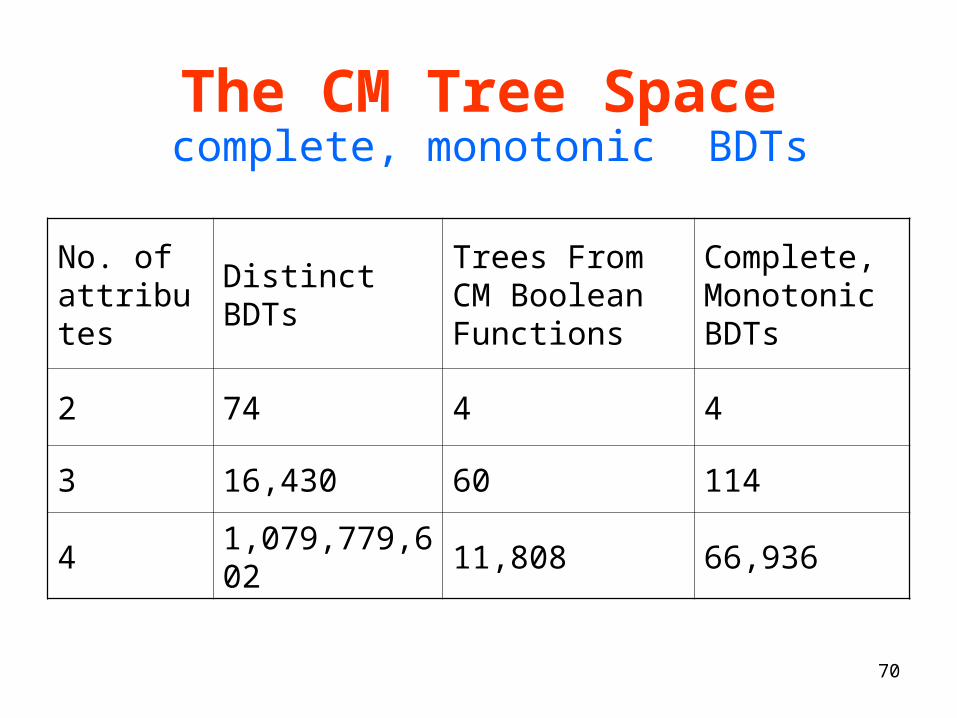
The CM Tree Space
No. of attributes
Distinct BDTsTrees From CM Boolean Functions
Complete, Monotonic BDTs
2 74 4 4
3 16,430 60 114
4 1,079,779,602 11,808 66,936
complete, monotonic BDTs

71
Tree Neighborhood and Tree Space• Define tree neighborhood by giving operations for
moving from one tree in CM Tree Space to another.• Structure-based methods• Classifications-based methods• We choose structure-based neighborhood methods
because the cost of a BDT depends more on its structure • Small changes in tree structure don’t significantly affect
cost, and… • All BDTs with the same Boolean functions may differ a
lot in cost

72
Search Operations in Tree Space
• Split Pick a leaf node and replace it with a sensor that is
not already present in that branch, and then insert arcs from that sensor to 0 and to 1.
a
b c
0 c d 1
d 1 0 1
0 1
SPLIT
a
b c
0 c d 1
d 1 b 1
0 1 0 1

73
Search Operations• Swap
Pick a non-leaf node in the tree and swap it with its parent node such that the new tree is still monotonic and complete and no sensor occurs more than once in any branch.
a
b c
0 c d 1
d 1 0 1
0 1
SWAP
a
b c
0 d d 1
c 1 0 1
0 1

74
Search Operations• Merge
Pick a parent node of two leaf nodes and make it a leaf node by collapsing the two leaf nodes below it, or pick a parent node with one leaf node, collapse both the parent node and its one leaf node, and shift the sub-tree up in the tree by one level.
a
b c
0 c d 1
d 1 0 1
0 1
MERGE
a
b c
0 d d 1
0 1 0 1
a
b c
0 c d 1
0 1 0 1

75
Search Operations• Replace
Pick a node with a sensor occurring more than once in the tree and replace it with any other sensor such that no sensor occurs more than once in any branch.
a
b c
0 c d 1
d 1 0 1
0 1
REPLACE
a
b c
0 c b 1
d 1 0 1
0 1

76

77
Tree Neighborhood and Tree Space
• Define tree neighborhood by using these four operations for moving from one tree in CM Tree Space to another.
• Irreducibility– Theorem: Any tree in the CM tree space can be
reached from any other tree by using these neighborhood operations repetitively
– An irreducible CM tree space helps “search” for the cheapest trees using neighborhood operations

78
Tree Space Traversal• Greedy Search
1. Randomly start at any tree in the CM tree space2. Find its neighboring trees using the above
operations3. Move to the neighbor with the lowest cost4. Iterate until we find a minimum
– The CM Tree space is highly multi-modal (more than one minimum)!
– Therefore, we implement a stochastic search algorithm with simulated annealing to find the best tree

79
Tree Space Traversal
• Stochastic Search– Randomly start at any tree in CM space– Find its neighboring trees, and evaluate each one for its
total cost– Select next move according to a probability distribution
over the neighboring trees
• To deal with the multimodality of the tree space, we introduce Simulated Annealing:– Make more random jumps initially, gradually decrease the
randomness and finally converge at the overall minimum

80
Tree Space Traversal• Stochastic Search
– Randomly start at any tree in CM space
– Find its neighboring trees, and evaluate each one for its total cost
– Select move according to a probability distribution over neighboring trees proportional to the ratio of the costs of two trees
– Specifically, if we are at the ith tree τi, then the probability of going to its kth neighbor, denoted τik, is given by
– where f(τj) and f(τij) are the costs of trees τi and τij, respectively and ni is the number of trees in the neighborhood of τij
– so-called “temperature” t is initiated to one and lowered in discrete unequal steps after every m hops until we reach a minimum
1
1
1
( ) ( )
( ) ( )i
t
i ikki n
t
i ijj
f fP
f f

81
Results: Searching CM Tree Space• We were able to perform experiments for 3, 4 and 5 sensors,
successfully• Results show improvement compared to the extensive search
method. E.g., for 4 sensors (66,936 trees)– 100 different experiments were performed– Each experiment was started 10 times randomly at some tree and chains
were formed by making stochastic moves in the neighborhood, until we find a local minimum
– Only 4890 trees were examined on average for every experiments– Global minimum was found 82 times while the second best tree was
found 10 times– The method found trees that were less costly than those found by earlier
searches of BDTs corresponding to complete, monotonic Boolean functions.

82
Genetic Algorithms-based Approach
• Structure-based neighborhood moves allow very short moves only. Therefore,…
• Techniques like Genetic Algorithms and Evolutionary Techniques may suggest ways for getting more efficiently to better trees, given a population of good trees

83
Genetic Algorithms-based Approach
• Started implementing genetic algorithms- based techniques for tree space traversal
• Basically, we try to get “better” trees from the current population of “good” trees using the basic genetic operations on them:– Selection– Crossover– Mutation
• Here, “better” decision trees correspond to lower cost decision trees than the ones in the current population (“good”).

84
Genetic Algorithms-based Approach• Therefore, as new trees are generated, the size of the
genePool keeps increasing.• Selection:
– Select an initial population of trees, bestPop, randomly out of the CM tree space
– Always keep a population of N best trees for further crossover and mutation operations
• Crossover: – Performed between every pair of trees in bestPop. – For each crossover operation between two trees τi and τj,
we randomly select nodes and exchange the subtrees

85
Genetic Algorithms-based Approach
• We randomly perform crossover operation k times between a pair of trees
• However, we impose certain restrictions to ensure that resultant trees lie in CM tree space

86
Genetic Algorithms-based Approach• Mutation:
– Performed after every m generations of the algorithm– We do two types of mutations:
• Generating all the neighboring trees of the current best population of trees using the four operations used in the stochastic search method and put them into the gene pool
• Replacing some fraction of the trees of bestPop with random samples from the CM tree space which are not in the gene pool
– Only ~1600 trees had to be examined to obtain the 10 best trees for 4 sensors!

87
Discussion and Future Work• Very few optimal trees; optimality insensitive to changes in
parameters.
• The extensive search techniques become practically infeasible beyond a very small number of sensors
• The new threshold optimization algorithms provide faster ways to arrive at a low tree cost; cost is lower and often much lower than in extensive search
• The irreducible tree space helps us to “search” for the best trees rather than evaluating all the trees for their cost
• The stochastic search algorithm allows us to search for optimum inspection schemes beyond 4 sensors successfully

88
Discussion and Future Work• Future work: Because of the rapid growth in
number of trees in CM Tree Space when the number of sensors grows, it is necessary to try to reduce the number of trees we need to search through.
• A notion of tree equivalence could be incorporated when the number of sensors go beyond 5 or 6
• We hope that incorporating this into our model will enable us to extend our model to a large number of sensors

89
Tree Equivalence and Tree Irreducibility
• A decision tree in CM tree space can be exactly equivalent to another decision tree in the CM tree space:
• This property is called transposition and the two trees are called transposes of each others

90
Tree Equivalence and Tree Irreducibility
• The problem is that the size of the equivalence class (number of transposes for a given tree) increases exponentially with the number of sensors.
• Therefore, we need to define a “canonical” representation of the equivalence class and deal with the equivalence class as a whole rather than treating each individual tree separately
91
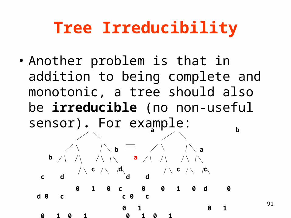
Tree Irreducibility
• Another problem is that in addition to being complete and monotonic, a tree should also be irreducible (no non-useful sensor). For example:
a
b b
c d c d
0 1 0 c 0 d 0 c
0 1 0 1 0 1
b
a a
c c d d
0 1 0 d 0 c 0 c
0 1 0 1 0 1

92
Discussion and Future Work•Future work: Need for more complicated cost models; bringing in costs of delays

93
Discussion and Future Work•Future work: More than two values of an attribute
(present, absent, present with probability > 75%, absent with probability at least 75%) (ok, not ok, ok with probability > 99%, ok with probability between 95% and 99%)
•Future work: In the Boolean function model: inferring the Boolean function from observations (partially defined Boolean functions)

94
Discussion and Future Work•Future Work: Explain why conclusions are so insensitive to variation in parameter values.•Future Work: Explore the structure of the optimal trees and compare the different optimal trees.•Future Work: Develop methods for approximating the optimal tree.
Pallet vacis

95
Closing Remark•Recall that the “cost” of inspection includes the cost of failure, including failure to foil a terrorist plot.•There are many ways to lower the total “cost” of inspection:
Use more efficient orders of inspection.Find ways to inspect more containers.Find ways to cut down on delays at inspection lanes.

96
Research Team• Tayfur Altiok, Rutgers, Ind. & Systems Engineering• Saket Anand, Rutgers, ECE graduate student• Endre Boros, Rutgers, Operations Research• Elsayed Elsayed, Rutgers, Ind. & Systems Engineering• Liliya Fedzhora, Rutgers, Operations Res. grad. student• Paul Kantor, Rutgers, Schl. of Infor. & Library Studies• Abdullah Karaman, Rutgers Ind. & Syst. Eng. grad. student• David Madigan, Rutgers, Statistics• Richard Mammone, Rutgers, Center for Advanced Information Processing• Ben Melamed, Rutgers Business School• Sushil Mittal, Rutgers, ECE graduate student• S. Muthukrishnan, Rutgers, Computer Science• Saumitr Pathek, Rutgers ECE graduate student• Richard Picard, Los Alamos, Statistical Sciences Group• Fred Roberts, Rutgers, DIMACS Center• Kevin Saeger, Los Alamos, Homeland Security• Christina Schroepfer, Rutgers, Ind. & Syst. Eng. Grad. student• Phillip Stroud, Los Alamos, Systems Engineering and Integration Group• Minge Xie, Rutgers, Statistics• Hao Zhang, Rutgers Ind. & Systems Eng., graduate student

97
Collaborators on Work Described:• Saket Anand• David Madigan• Richard Mammone• Sushil Mittal*• Saumitr Pathak
Research Support: • Office of Naval Research• National Science Foundation• New support: Domestic Nuclear Detection Office
Los Alamos National Laboratory:• Rick Picard• Kevin Saeger• Phil Stroud