1-800-582-2763 · hASF uud.dOtdn gdekddOSwSt.ron ... with 95% confidence, you have no more than a...
6
Transcript of 1-800-582-2763 · hASF uud.dOtdn gdekddOSwSt.ron ... with 95% confidence, you have no more than a...

www.casioeducation.com 1-800-582-2763
StatFinalCVR1,4.indd 1 8/23/11 6:14 AM

C A S I O | w w w. C A S I O e d u C At I O n . C O m
4. UNIVARIATE
INFEREN
CES
4. UNIVARIATE
INFEREN
CES
1. DESCRIPTIVE
TECHNIQ
UES
3. NORM
ALDISTRIBU
TION
5. REGRESSION MODELS
AND ANALYSIS6. D
IFFERENCES
BETWEEN
2 CROPS
7. ANOVA AN
DCH
I-SQUARE
8. EXTENDING STATISTICAL THINKING
2. COUNTING AND THEBINOM
IAL DISTRIBUTION
1. DESCRIPTIVE
TECHNIQ
UES
3. NORM
ALDISTRIBU
TION
5. REGRESSION MODELS
AND ANALYSIS6. D
IFFERENCES
BETWEEN
2 CROPS
7. ANOVA AN
DCH
I-SQUARE
8. EXTENDING STATISTICAL THINKING
2. COUNTING AND THEBINOM
IAL DISTRIBUTION
INTRO
DUCTIO
NDATA EN
TRY
INTRO
DUCTIO
NDATA EN
TRY
Investigation 4.2: a Warming World
Carbon Dioxide and methane are the main greenhouse gases contributing to global warming. over the last century the
earth has warmed approximately 1 degree Fahrenheit. the multinational Arctic Climate impact Assessment (ACiA) report concludes that in Alaska, western Canada, and eastern russia, average temperatures
have increased as much as 4 to 7 degrees Fahrenheit (3 to 4 degrees Celsius) in the past 50 years. the decade ending in 2009 was the warmest on record.Reference: http://climatechange.ws/facts/
You are curious about the proportion of Americans who believe that global warming is due to human activity. According to one study, the proportion is ap-proximately 45%.
A. if this is the case, how many people must be included in a study to en-sure that, with 95% confidence, you have no more than a 3% error?
b. For what value of π (proportion of the population) is the standard error the greatest? explain. Use this value to answer Part A above. How many more people would you need in your sample size in this “worst case” scenario?
C. Assuming you want 95% confidence in your results, explore the relation-ship between the total error and the sample size. Assume the worst case. Discuss your findings.
Reference: http://www.rasmussenreports.com/public_content/politics/current_events/ environment_energy/energy_update
C A S I O | P u t vA l u e b A C k I n t h e e q u At I O n
4. UNIVARIATE
INFEREN
CES
4. UNIVARIATE
INFEREN
CES
1. DESCRIPTIVE
TECHNIQ
UES
3. NORM
ALDISTRIBU
TION
5. REGRESSION MODELS
AND ANALYSIS6. D
IFFERENCES
BETWEEN
2 CROPS
7. ANOVA AN
DCH
I-SQUARE
8. EXTENDING STATISTICAL THINKING
2. COUNTING AND THEBINOM
IAL DISTRIBUTION
1. DESCRIPTIVE
TECHNIQ
UES
3. NORM
ALDISTRIBU
TION
5. REGRESSION MODELS
AND ANALYSIS6. D
IFFERENCES
BETWEEN
2 CROPS
7. ANOVA AN
DCH
I-SQUARE
8. EXTENDING STATISTICAL THINKING
2. COUNTING AND THEBINOM
IAL DISTRIBUTION
INTRO
DUCTIO
NDATA EN
TRY
INTRO
DUCTIO
NDATA EN
TRY
One Solution: a Warming WorldA. if this is the case, how many people must be included in a study to
ensure that, with 95% confidence, you have no more than a 3% error?The total error is given by the product of the standard error and the confidence coefficient. The standard error of the sampling distribution for a confidence interval of a categorical variable is given by the formula , where π represents the proportion of the population who believe this (here it is not the value approximated by 3.14). Since we are to assume that 0.45 is the correct value for π, we will use it in the formula.
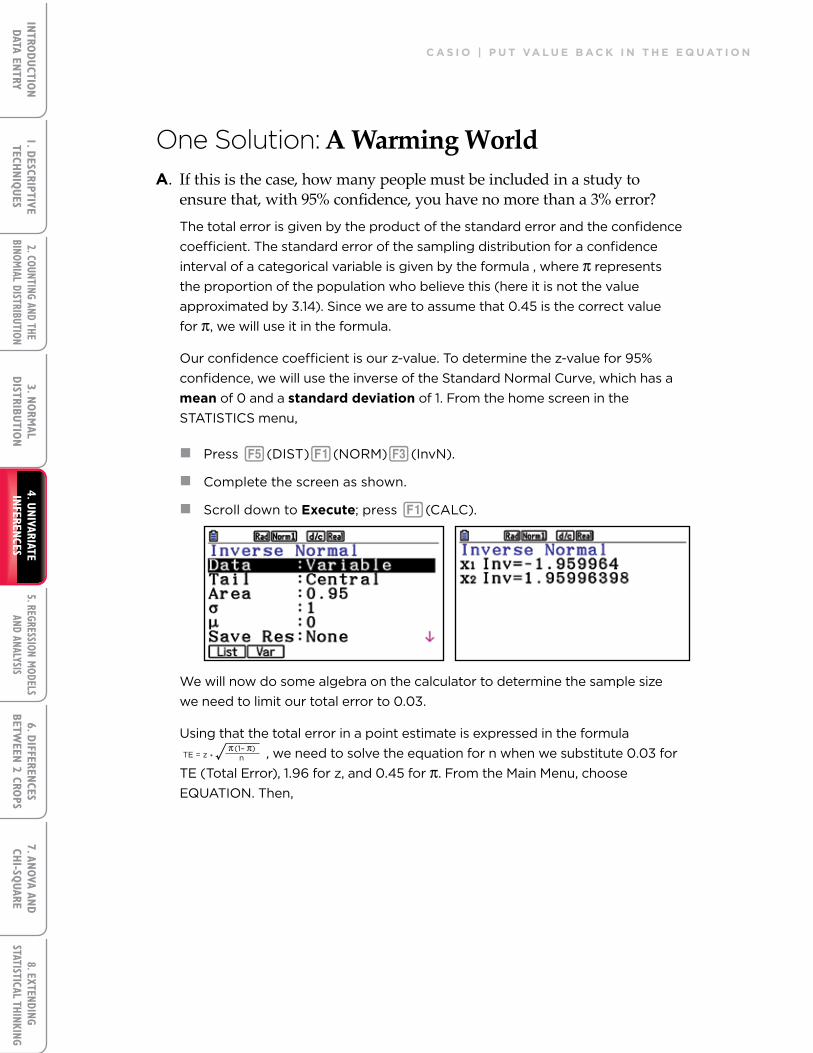
Our confidence coefficient is our z-value. To determine the z-value for 95% confidence, we will use the inverse of the Standard Normal Curve, which has a mean of 0 and a standard deviation of 1. From the home screen in the STATISTICS menu,
n Press y(DIST)q(NORM)e(InvN).
n Complete the screen as shown.
n Scroll down to execute; press q(CALC).
We will now do some algebra on the calculator to determine the sample size we need to limit our total error to 0.03.
Using that the total error in a point estimate is expressed in the formula TE = z * n
π π(1– ) , we need to solve the equation for n when we substitute 0.03 for TE (Total Error), 1.96 for z, and 0.45 for π. From the Main Menu, choose EQUATION. Then,
C A S I O | w w w. C A S I O e d u C At I O n . C O m
4. UNIVARIATE
INFEREN
CES
4. UNIVARIATE
INFEREN
CES
1. DESCRIPTIVE
TECHNIQ
UES
3. NORM
ALDISTRIBU
TION
5. REGRESSION MODELS
AND ANALYSIS6. D
IFFERENCES
BETWEEN
2 CROPS
7. ANOVA AN
DCH
I-SQUARE
8. EXTENDING STATISTICAL THINKING
2. COUNTING AND THEBINOM
IAL DISTRIBUTION
1. DESCRIPTIVE
TECHNIQ
UES
3. NORM
ALDISTRIBU
TION
5. REGRESSION MODELS
AND ANALYSIS6. D
IFFERENCES
BETWEEN
2 CROPS
7. ANOVA AN
DCH
I-SQUARE
8. EXTENDING STATISTICAL THINKING
2. COUNTING AND THEBINOM
IAL DISTRIBUTION
INTRO
DUCTIO
NDATA EN
TRY
INTRO
DUCTIO
NDATA EN
TRY
A wARmIng wORld
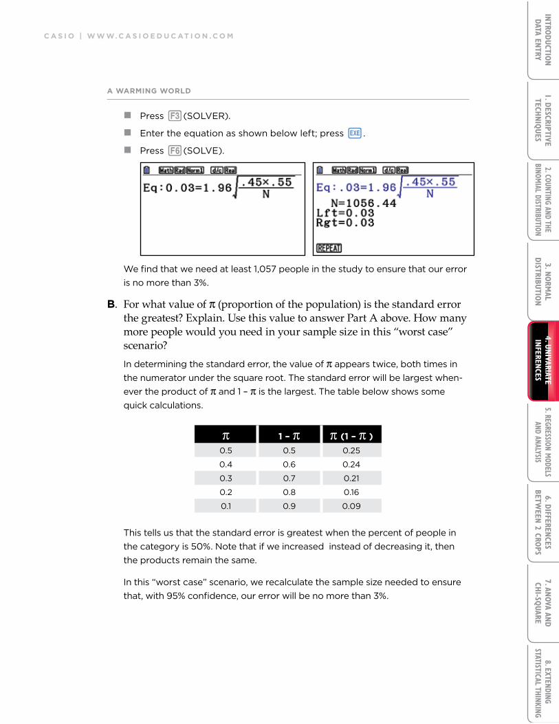
n Press e(SOLVER).
n Enter the equation as shown below left; press l.
n Press u(SOLVE).
We find that we need at least 1,057 people in the study to ensure that our error is no more than 3%.
b. For what value of π (proportion of the population) is the standard error the greatest? explain. Use this value to answer Part A above. How many more people would you need in your sample size in this “worst case” scenario?In determining the standard error, the value of π appears twice, both times in the numerator under the square root. The standard error will be largest when-ever the product of π and 1 – π is the largest. The table below shows some quick calculations.
π 1 – π π (1 – π )
0.5 0.5 0.25
0.4 0.6 0.24
0.3 0.7 0.21
0.2 0.8 0.16
0.1 0.9 0.09
This tells us that the standard error is greatest when the percent of people in the category is 50%. Note that if we increased instead of decreasing it, then the products remain the same.
In this “worst case” scenario, we recalculate the sample size needed to ensure that, with 95% confidence, our error will be no more than 3%.
C A S I O | P u t vA l u e b A C k I n t h e e q u At I O n
4. UNIVARIATE
INFEREN
CES
4. UNIVARIATE
INFEREN
CES
1. DESCRIPTIVE
TECHNIQ
UES
3. NORM
ALDISTRIBU
TION
5. REGRESSION MODELS
AND ANALYSIS6. D
IFFERENCES
BETWEEN
2 CROPS
7. ANOVA AN
DCH
I-SQUARE
8. EXTENDING STATISTICAL THINKING
2. COUNTING AND THEBINOM
IAL DISTRIBUTION
1. DESCRIPTIVE
TECHNIQ
UES
3. NORM
ALDISTRIBU
TION
5. REGRESSION MODELS
AND ANALYSIS6. D
IFFERENCES
BETWEEN
2 CROPS
7. ANOVA AN
DCH
I-SQUARE
8. EXTENDING STATISTICAL THINKING
2. COUNTING AND THEBINOM
IAL DISTRIBUTION
INTRO
DUCTIO
NDATA EN
TRY
INTRO
DUCTIO
NDATA EN
TRY
A wARmIng wORld
From the screen shown above right,
n Press q(REPEAT).
n Use the scroll bar and change the product of 0.45 x 0.55 to 0.50 x 0.50.
n Press lu(SOLVE).
We find that we need at least 1,068 people in the study to ensure that, with 95% confidence, our error will not exceed 3%. This is a modest increase of only 11 people in the study.
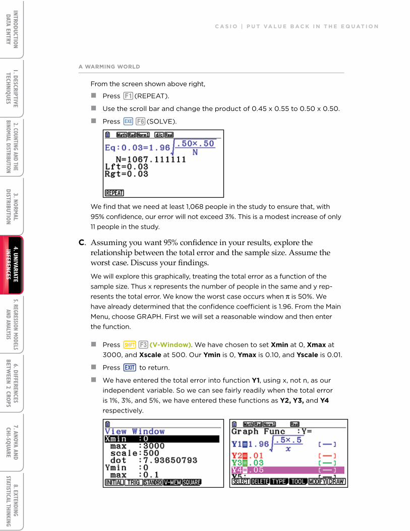
C. Assuming you want 95% confidence in your results, explore the relationship between the total error and the sample size. Assume the worst case. Discuss your findings. We will explore this graphically, treating the total error as a function of the sample size. Thus x represents the number of people in the same and y rep-resents the total error. We know the worst case occurs when π is 50%. We have already determined that the confidence coefficient is 1.96. From the Main Menu, choose GRAPH. First we will set a reasonable window and then enter the function.
n Press Le(v-window). We have chosen to set xmin at 0, xmax at 3000, and xscale at 500. Our ymin is 0, ymax is 0.10, and yscale is 0.01.
n Press d to return.
n We have entered the total error into function y1, using x, not n, as our independent variable. So we can see fairly readily when the total error is 1%, 3%, and 5%, we have entered these functions as y2, y3, and y4 respectively.

C A S I O | w w w. C A S I O e d u C At I O n . C O m
4. UNIVARIATE
INFEREN
CES
4. UNIVARIATE
INFEREN
CES
1. DESCRIPTIVE
TECHNIQ
UES
3. NORM
ALDISTRIBU
TION
5. REGRESSION MODELS
AND ANALYSIS6. D
IFFERENCES
BETWEEN
2 CROPS
7. ANOVA AN
DCH
I-SQUARE
8. EXTENDING STATISTICAL THINKING
2. COUNTING AND THEBINOM
IAL DISTRIBUTION
1. DESCRIPTIVE
TECHNIQ
UES
3. NORM
ALDISTRIBU
TION
5. REGRESSION MODELS
AND ANALYSIS6. D
IFFERENCES
BETWEEN
2 CROPS
7. ANOVA AN
DCH
I-SQUARE
8. EXTENDING STATISTICAL THINKING
2. COUNTING AND THEBINOM
IAL DISTRIBUTION
INTRO
DUCTIO
NDATA EN
TRY
INTRO
DUCTIO
NDATA EN
TRY
A wARmIng wORld
n Press u(DRAW) to see the graphs.
The blue graph, which represents the total error, shows that as we move to the right (adding more people to the sample), at first the total error drops dramati-cally. It then levels off; we reach a point when adding more people has only a small effect upon the total error. Even at the far right end of the graph, when the sample size is 3000, the total error is still greater than 1% (note the blue curve never gets as low as the red line). It appears that if we want the total error limited to 2%, we would need approximately 2,500 people in the study. Earlier we found that with 1,068 people in the study, our total error is 3%. Thus we would have to more than double the sample size to reduce the error from 3% to 2%. Perhaps this will help students understand why many major studies often use a little more than 1,000 people in their surveys.
To see how many people we would need if we would accept an error of 5%,
n Press Ly(g-Solv)y(INTSECT).
n Press l when y1 and y4 are highlighted.
We see that we need only 385 people in the study if we are willing to accept an error of 5%.