1

2

OverviewOverview Suffix tries On-line construction of suffix tries in

quadratic time Suffix trees On-line construction of suffix trees in

linear time Applications

3

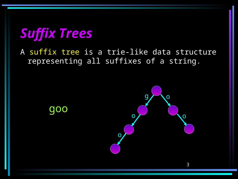
Suffix TreesSuffix TreesA suffix tree is a trie-like data structure

representing all suffixes of a string.

g

o

o

o

o

goo

4

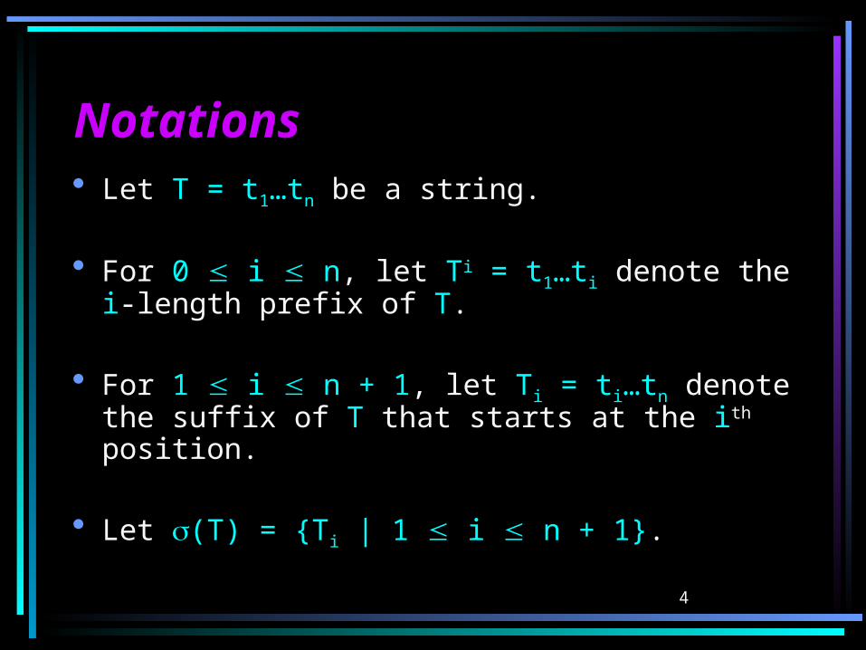
NotationsNotations Let T = t1…tn be a string.

For 0 i n, let Ti = t1…ti denote thei-length prefix of T.

For 1 i n + 1, let Ti = ti…tn denote the suffix of T that starts at the ith position.

Let (T) = {Ti | 1 i n + 1}.

5

Suffix TriesSuffix TriesThe suffix trie of T, denoted by STrie(T), is

a trie representing (T).

6

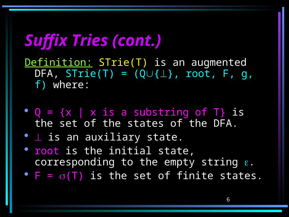
Suffix Tries (cont.)Suffix Tries (cont.)Definition: STrie(T) is an augmented DFA,

STrie(T) = (Q{}, root, F, g, f) where:

Q = {x | x is a substring of T} is the set of the states of the DFA.

is an auxiliary state. root is the initial state, corresponding to

the empty string . F = (T) is the set of finite states.

7

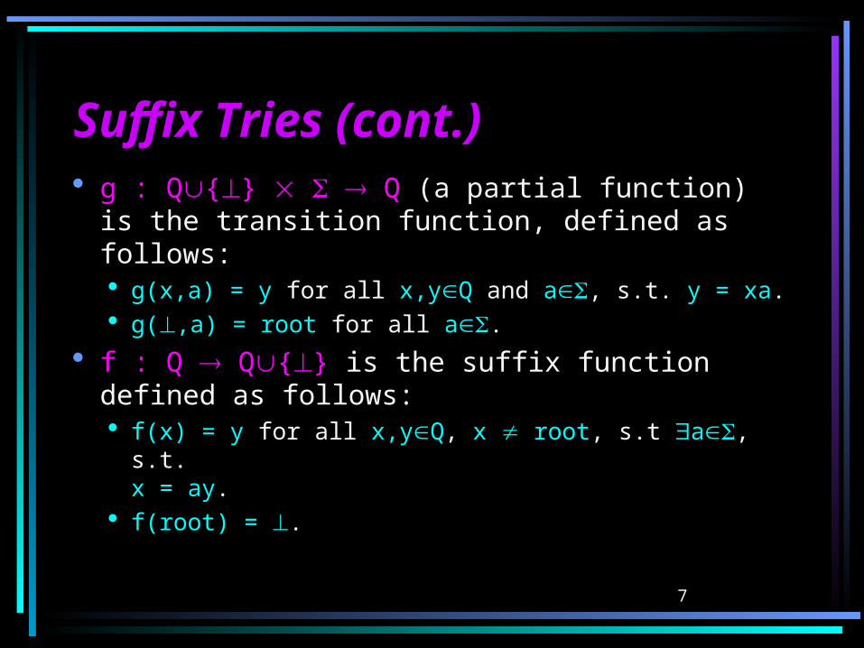
Suffix Tries (cont.)Suffix Tries (cont.) g : Q{} Q (a partial function) is

the transition function, defined as follows: g(x,a) = y for all x,yQ and a, s.t. y = xa. g(,a) = root for all a.

f : Q Q{} is the suffix function defined as follows: f(x) = y for all x,yQ, x root, s.t a, s.t.

x = ay. f(root) = .

8

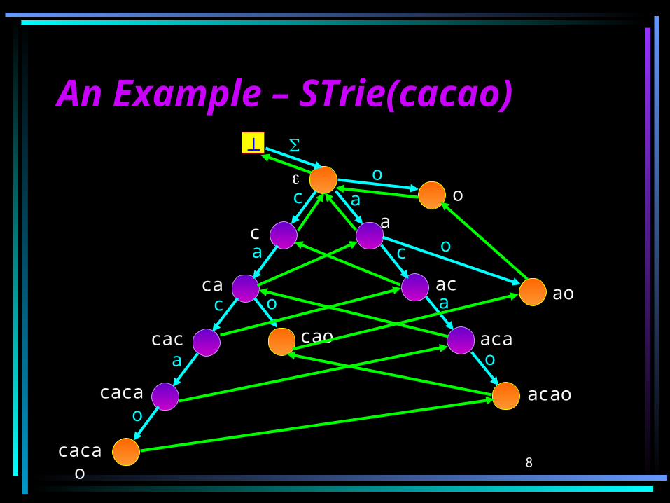
An Example – STrie(cacao)An Example – STrie(cacao)

cacao

aca

acao

ao

c

cac

caca

cao

ca

oa

ac

o

a

a c

c

c

o

o

o

o

a

a

9

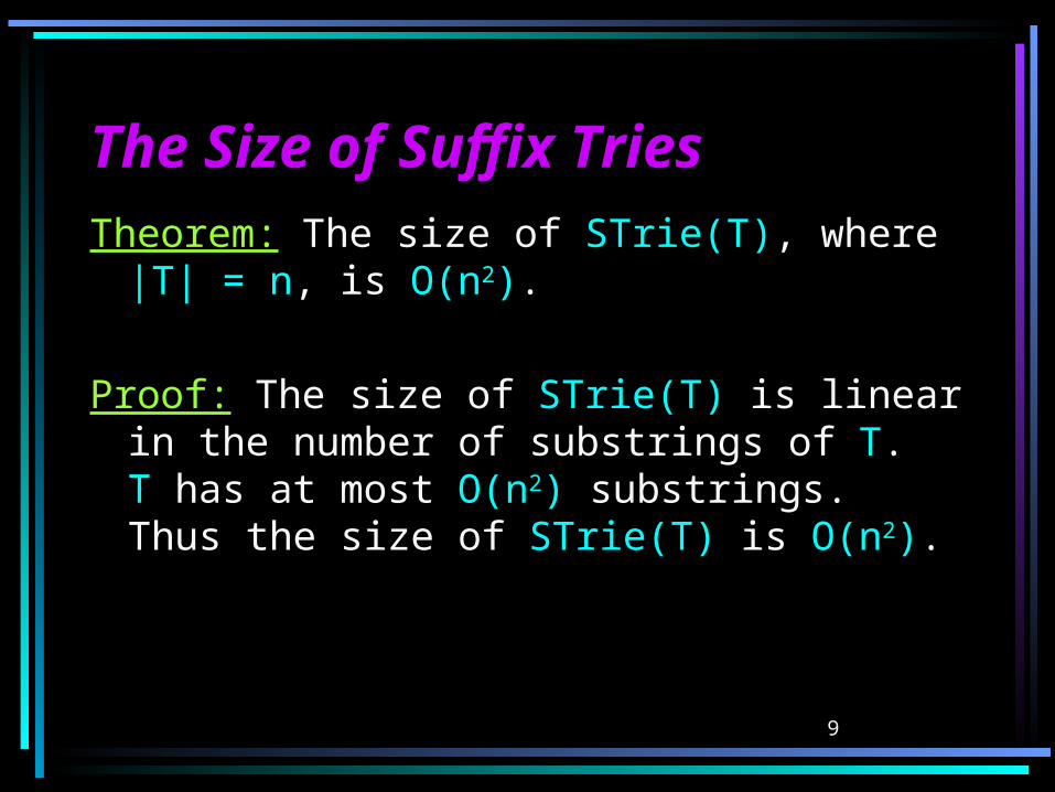
The Size of Suffix TriesThe Size of Suffix TriesTheorem: The size of STrie(T), where

|T| = n, is O(n2).

Proof: The size of STrie(T) is linear in the number of substrings of T.T has at most O(n2) substrings. Thus the size of STrie(T) is O(n2).

10

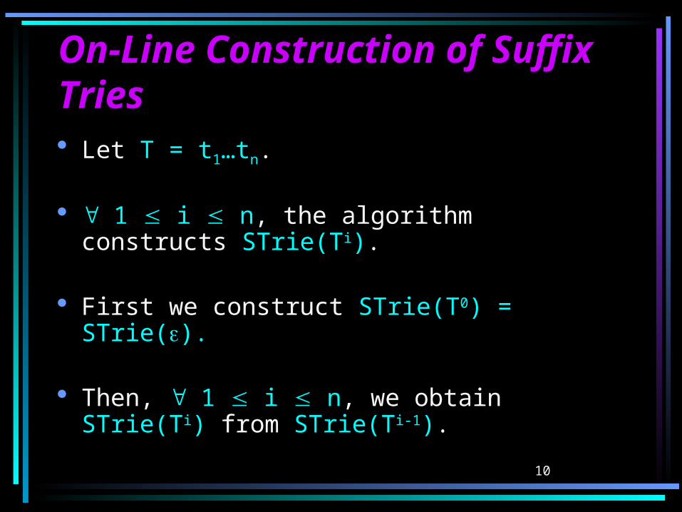
On-Line Construction of On-Line Construction of Suffix TriesSuffix Tries Let T = t1…tn.

1 i n, the algorithm constructs STrie(Ti).

First we construct STrie(T0) = STrie().

Then, 1 i n, we obtain STrie(Ti) from STrie(Ti-1).

11

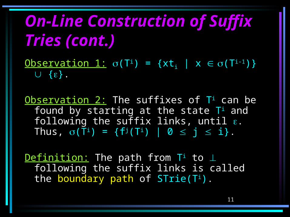
On-Line Construction of On-Line Construction of Suffix Tries (cont.)Suffix Tries (cont.)Observation 1: (Ti) = {xti | x (Ti-1)} {}.

Observation 2: The suffixes of Ti can be found by starting at the state Ti and following the suffix links, until .Thus, (Ti) = {fj(Ti) | 0 j i}.

Definition: The path from Ti to following the suffix links is called the boundary path of STrie(Ti).

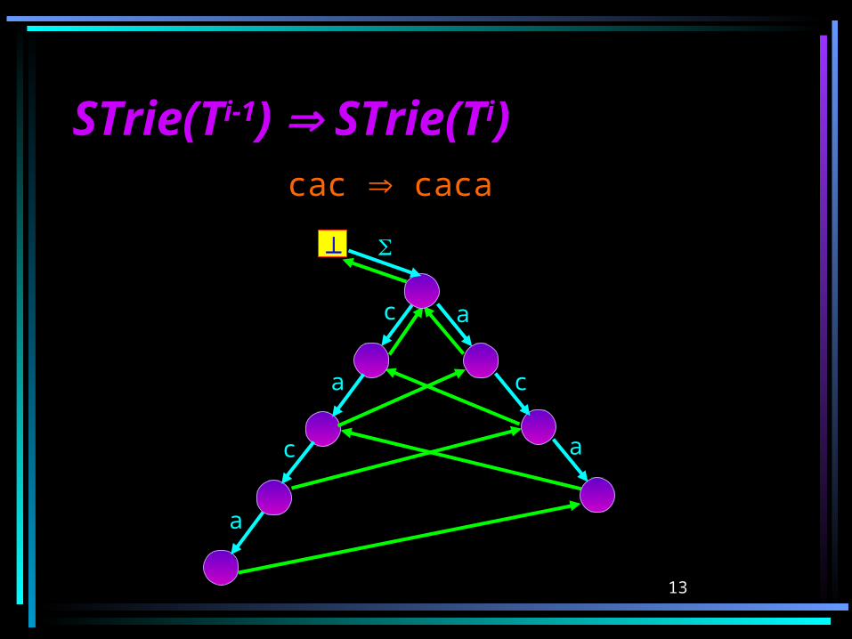
12

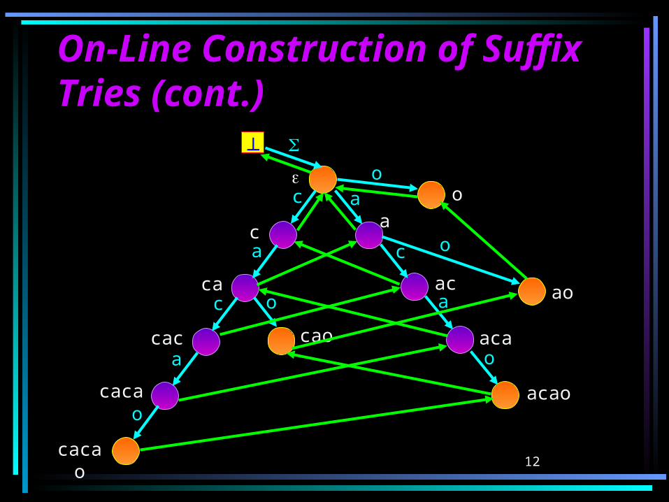
On-Line Construction of On-Line Construction of Suffix Tries (cont.)Suffix Tries (cont.)

cacao

aca

acao

ao

c

cac

caca

cao

ca

oa

ac

o

a

a c

c

c

o

o

o

o

a

a

13

a

STrie(TSTrie(Ti-1i-1) ) STrie(T STrie(Tii) )

a

c

a

a

c

c

cac caca

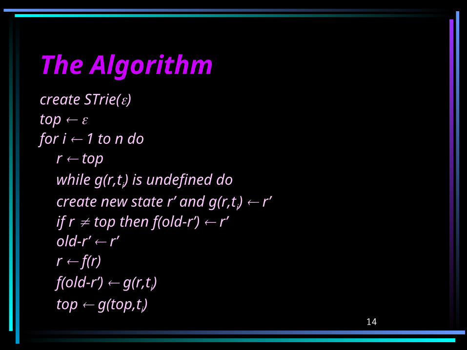
14

The AlgorithmThe Algorithmcreate STrie()top for i 1 to n do

r topwhile g(r,ti) is undefined do

create new state r’ and g(r,ti) r’if r top then f(old-r’) r’old-r’ r’r f(r)

f(old-r’) g(r,ti)

top g(top,ti)

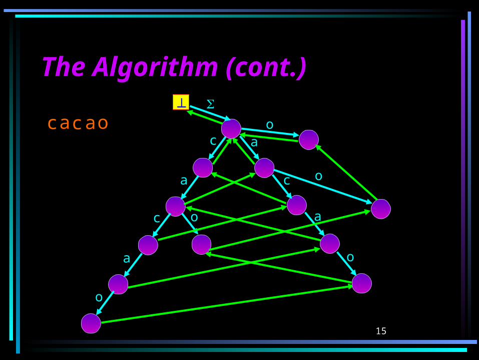
15

a

o

The Algorithm (cont.)The Algorithm (cont.)

c

a

a

c

ac

o

o

o

o

c ocaa

16

Running TimeRunning TimeTheorem: The running time of the

algorithm is linear in the size of STrie(T), which is, in worst case, O(|T|2).

17

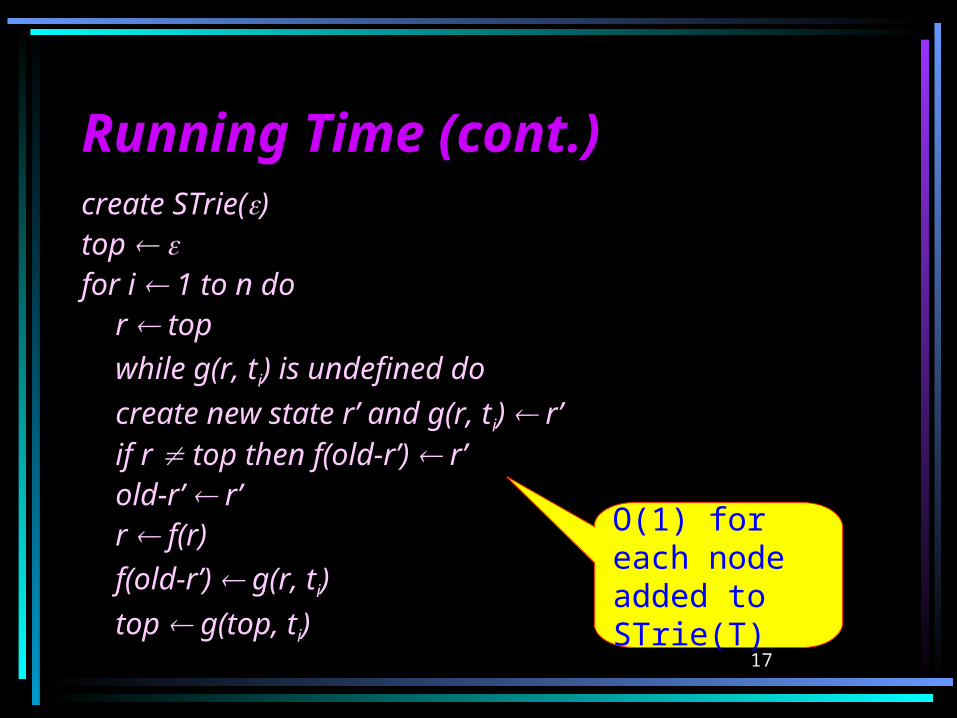
Running Time (cont.)Running Time (cont.)create STrie()top for i 1 to n do

r topwhile g(r, ti) is undefined do

create new state r’ and g(r, ti) r’if r top then f(old-r’) r’old-r’ r’r f(r)

f(old-r’) g(r, ti)

top g(top, ti)

O(1) for each node added to STrie(T)

18

Suffix TreesSuffix Trees A suffix tree STree(T) represents

STrie(T) in space linear in |T|.

This is achieved by representing only a subset of Q’{} of Q{}, called the explicit states.

19

Explicit and Implicit Explicit and Implicit StatesStatesDefinition: A state q is called explicit in

the following cases: q is a leaf q is a branching state (has at least two

transitions) root and are also defined to be branching

states.

Otherwise (if q has exactly one transitions and is not the root or ), q is called implicit.

20

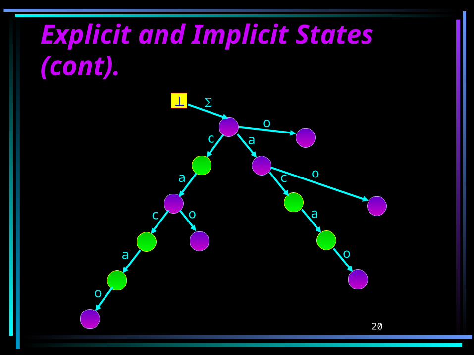
Explicit and Implicit Explicit and Implicit States (cont).States (cont).

a

o

c

a

a

c

ac

o

o

o

o

21

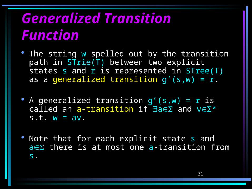
Generalized Transition Generalized Transition FunctionFunction The string w spelled out by the transition

path in STrie(T) between two explicit states s and r is represented in STree(T) as a generalized transition g’(s,w) = r.

A generalized transition g’(s,w) = r is called an a-transition if a and v* s.t. w = av.

Note that for each explicit state s and a there is at most one a-transition from s.

22

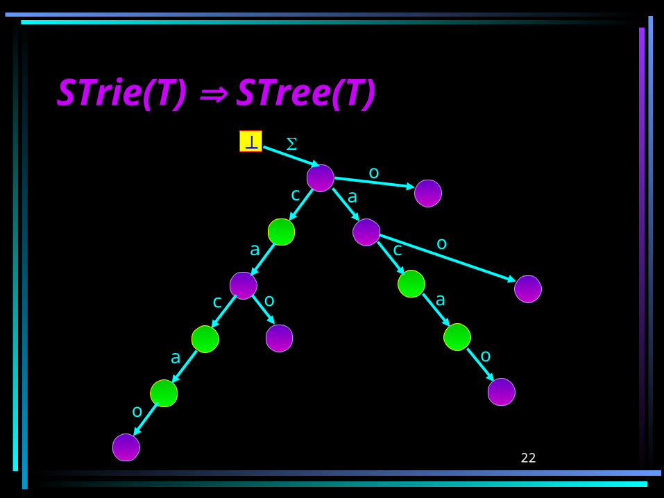
STrie(T) STrie(T) STree(T) STree(T)

a

o

c

a

a

c

ac

o

o

o

o

23

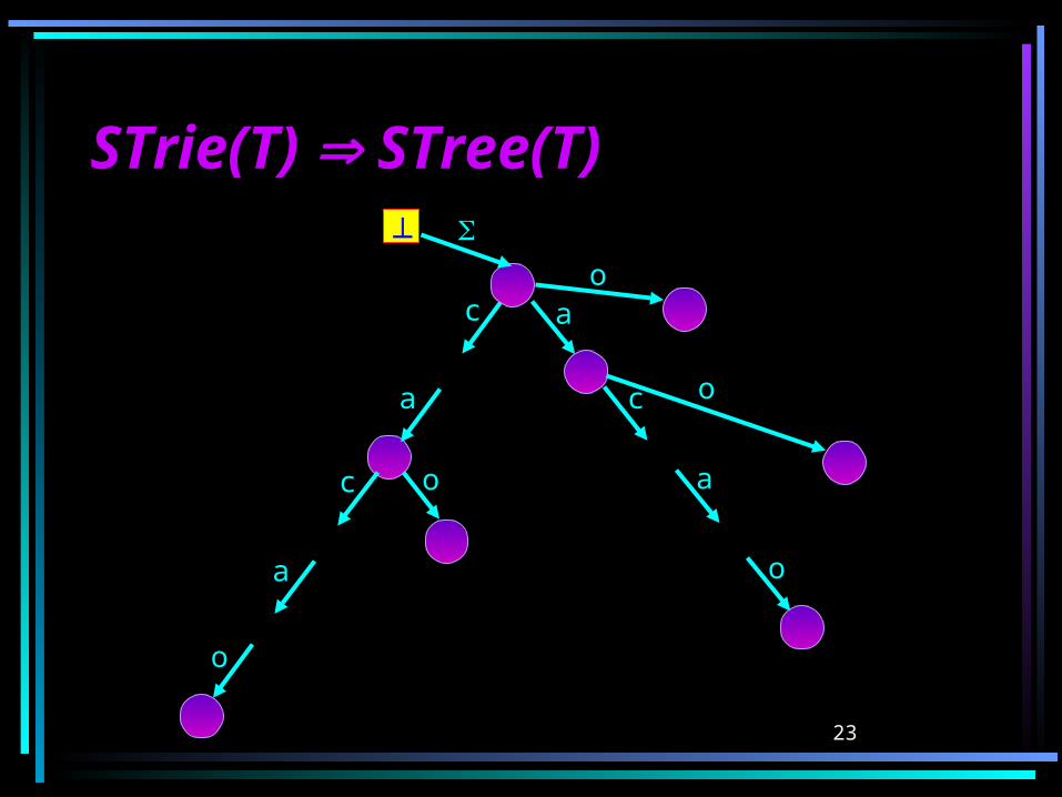
STrie(T) STrie(T) STree(T) STree(T)

a

o

c

a

a

c

ac

o

o

o

o

24

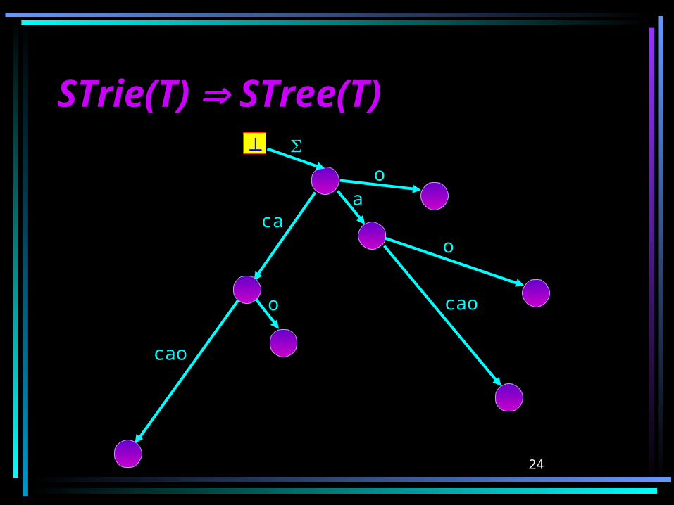
STrie(T) STrie(T) STree(T) STree(T)

cao

caa

cao

o

o

o

25

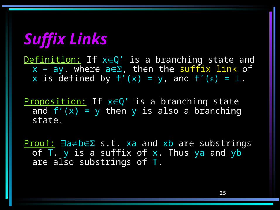
Suffix LinksSuffix LinksDefinition: If xQ’ is a branching state and

x = ay, where a, then the suffix link of x is defined by f’(x) = y, and f’() = .

Proposition: If xQ’ is a branching state and f’(x) = y then y is also a branching state.

Proof: ab s.t. xa and xb are substrings of T. y is a suffix of x. Thus ya and yb are also substrings of T.

26

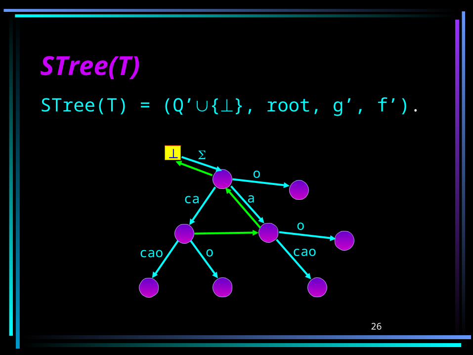
STree(T)STree(T)STree(T) = (Q’{}, root, g’, f’).

cao

ca a

cao

o

o

o

27

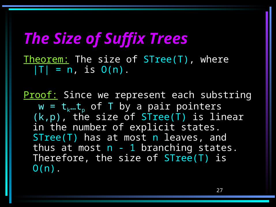
The Size of Suffix TreesThe Size of Suffix TreesTheorem: The size of STree(T), where

|T| = n, is O(n).

Proof: Since we represent each substring w = tk…tp of T by a pair pointers (k,p), the size of STree(T) is linear in the number of explicit states. STree(T) has at most n leaves, and thus at most n - 1 branching states. Therefore, the size of STree(T) is O(n).

28

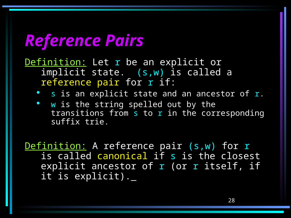
Reference PairsReference PairsDefinition: Let r be an explicit or implicit

state. (s,w) is called a reference pair for r if:

s is an explicit state and an ancestor of r. w is the string spelled out by the transitions

from s to r in the corresponding suffix trie.

Definition: A reference pair (s,w) for r is called canonical if s is the closest explicit ancestor of r (or r itself, if it is explicit).

29

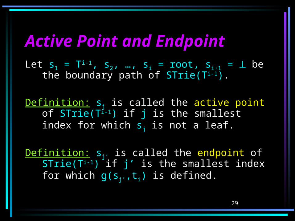
Active Point and EndpointActive Point and EndpointLet s1 = Ti-1, s2, …, si = root, si+1 = be the

boundary path of STrie(Ti-1).

Definition: sj is called the active point of STrie(Ti-1) if j is the smallest index for which sj is not a leaf.

Definition: sj’ is called the endpoint of STrie(Ti-1) if j’ is the smallest index for which g(sj’,ti) is defined.

30

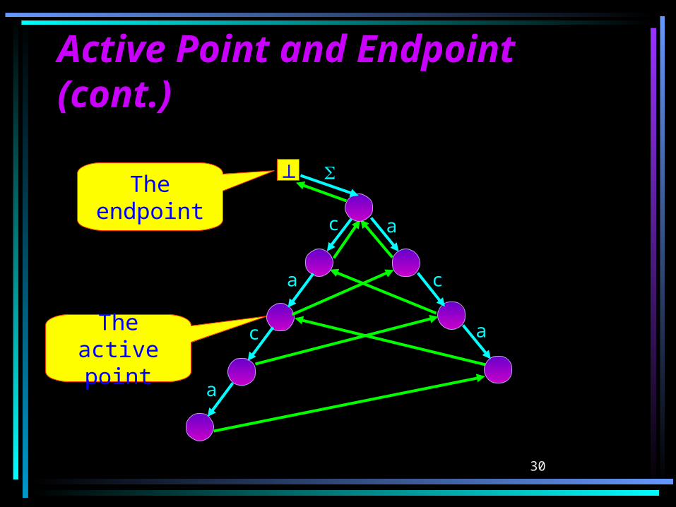
Active Point and Endpoint Active Point and Endpoint (cont.)(cont.)

The endpoint

The active point

a

a

c

a

a

c

c

31

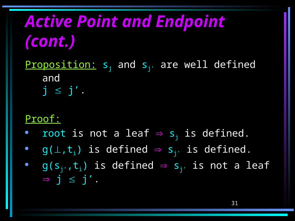
Active Point and Endpoint Active Point and Endpoint (cont.)(cont.)Proposition: sj and sj’ are well defined and

j j’.

Proof: root is not a leaf sj is defined.

g(,ti) is defined sj’ is defined.

g(sj’,ti) is defined sj’ is not a leaf j j’.

32

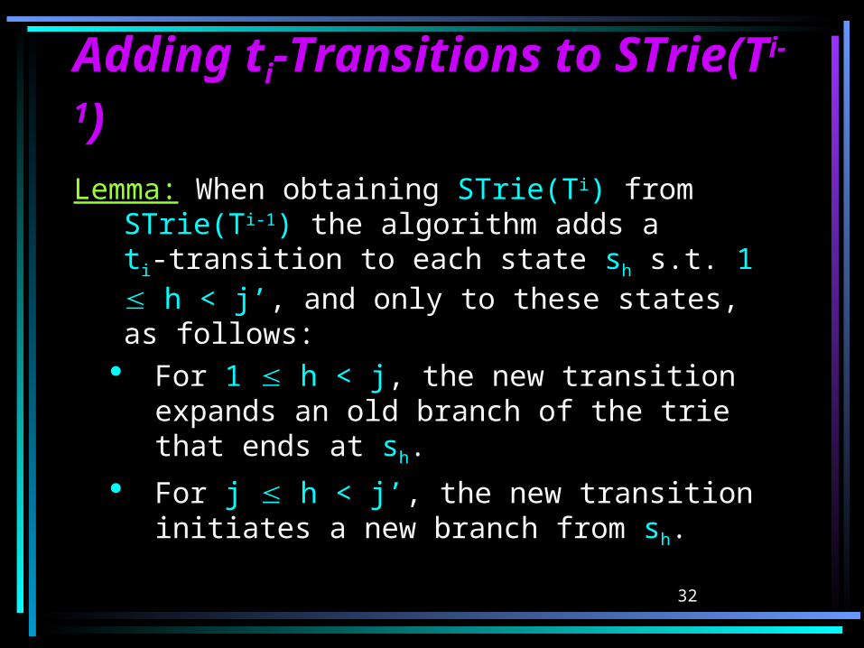
Adding tAdding tii-Transitions to -Transitions to STrie(TSTrie(Ti-1i-1))Lemma: When obtaining STrie(Ti) from

STrie(Ti-1) the algorithm adds ati-transition to each state sh s.t. 1 h < j’, and only to these states, as follows:

For 1 h < j, the new transition expands an old branch of the trie that ends at sh.

For j h < j’, the new transition initiates a new branch from sh.

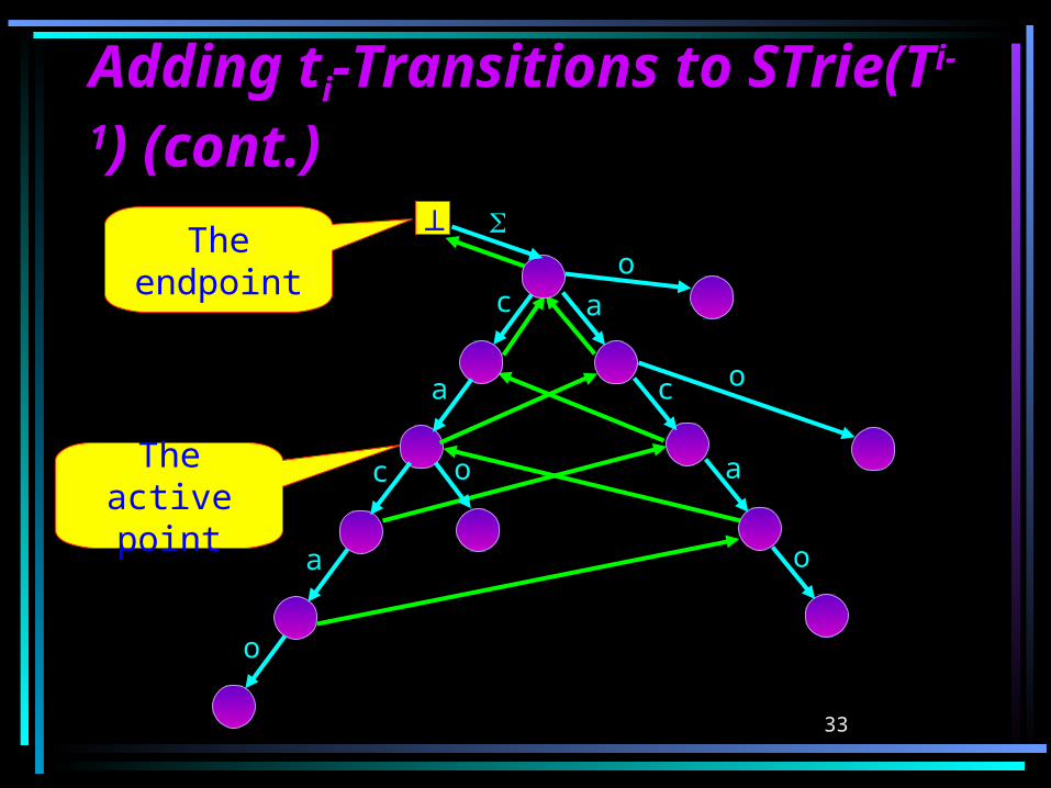
33

Adding tAdding tii-Transitions to -Transitions to STrie(TSTrie(Ti-1i-1) (cont.)) (cont.)

The endpoint

The active point

a

a

c

a

a

c

c

o

o

o

o

o

34

On-Line Construction of On-Line Construction of Suffix TreesSuffix Trees We create STree(), and then 1 i

n we obtain STree(Ti) from STree(Ti-1).

When obtaining STree(Ti) fromSTree(Ti-1), we update STree(Ti-1) according to the transitions we would add to STrie(Ti-1).

Note that s1,…,si-1 are not necessarily explicit states.

35

On-Line Construction of On-Line Construction of Suffix Trees (cont.)Suffix Trees (cont.)For 1 h < j:

sh is a leaf. Thus, s, 0 k i-1 s.t. g’(s,(k,i-1)) = sh. We replace this transition by g’(s,(k,i)) = sh.

This would take too much time. Thus, we denote transitions of the type g’(s,(k,i-1)) in STree(Ti-1) by g’(s,(k,)). Hence, no updates are needed.

36

On-Line Construction of On-Line Construction of Suffix Trees (cont.)Suffix Trees (cont.)For j h < j’:

If sh is an implicit state, we turn it into an explicit state by splitting the transition containing it.

We create a new leaf shti and add a new transition g’(sh,(i,)).

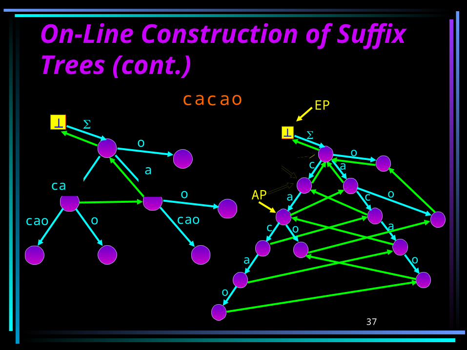
37

EP

EP

aacacaacao

a cca

cac

cacacacao

ca

On-Line Construction of On-Line Construction of Suffix Trees (cont.)Suffix Trees (cont.)

cao o cao

o

o

c ocaa

a

a

a

a

c

c

o

o

o

o

o

c

AP

AP

EP

EP

38

Lemma 1Lemma 1Lemma 1: Let (s,(k,p)) be some reference pair

for a state r. Then s’, k’ s.t. (s’,(k’,p)) is the canonical reference pair for r.

Proof: Let s’ be the closest explicit ancestor of r, or r itself if r is explicit. tk…tp is the path from the explicit state s to r. Thus, the path from s’ to r is a suffix tk’…tp of tk…tp.

39

Lemma 2Lemma 2Lemma 2: Let r be a state on the boundary

path of STrie(Ti). Then s, k s.t. (s,(k,i)) is the canonical reference pair for r.

Proof: r is on the boundary path of STrie(Ti). r refers to some suffix tk’…ti of Ti. (,(k’,i)) is a reference pair for r. the claim holds by lemma 1.

40

Lemma 3Lemma 3Lemma 3: Let (s,(k,i-1)) be a reference pair

for the endpoint of STrie(Ti-1). Then (s,(k,i)) is a reference pair for the active point of STrie(Ti).

Proof: sj is the active point of STrie(Ti-1) iff tj…

ti-1 is the longest suffix of Ti-1 that occurs at least twice in Ti-1.

41

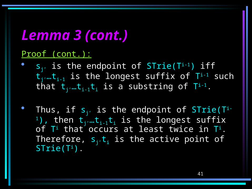
Lemma 3 (cont.)Lemma 3 (cont.)Proof (cont.): sj’ is the endpoint of STrie(Ti-1) iff tj’…ti-1 is

the longest suffix of Ti-1 such that tj’…ti-1ti is a substring of Ti-1.

Thus, if sj’ is the endpoint of STrie(Ti-1), then tj’…ti-1ti is the longest suffix of Ti that occurs at least twice in Ti. Therefore, sj’ti is the active point of STrie(Ti).

42

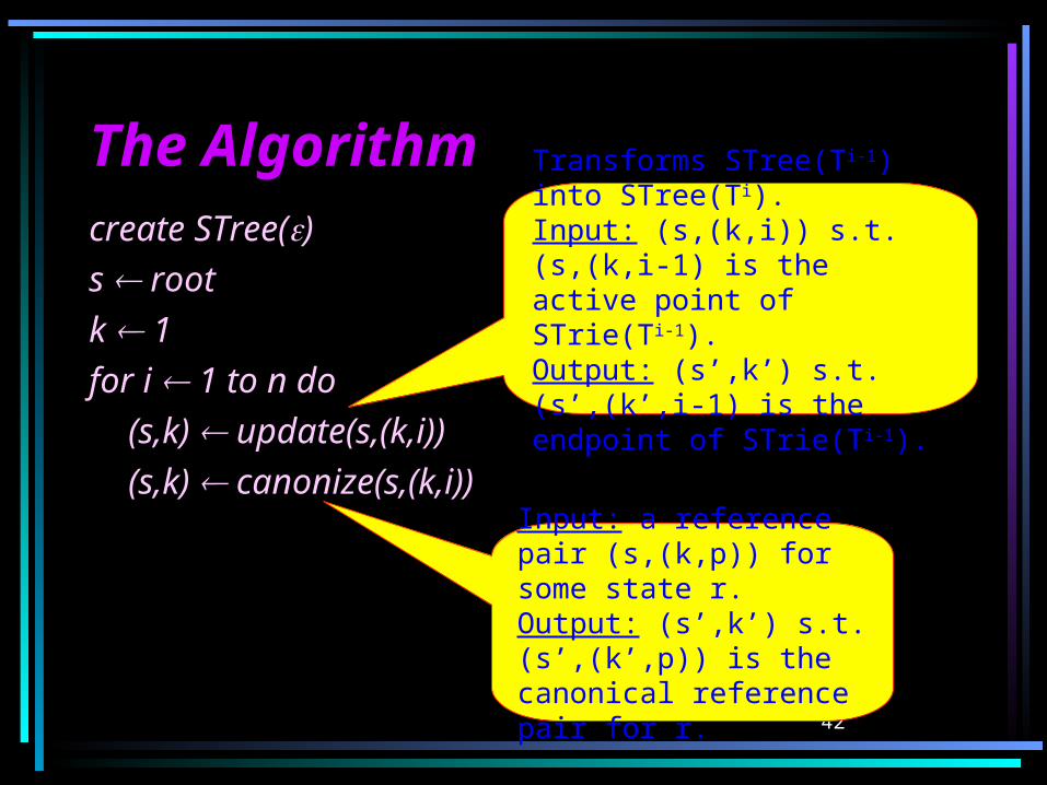
The AlgorithmThe Algorithmcreate STree()s rootk 1 for i 1 to n do

(s,k) update(s,(k,i))(s,k) canonize(s,(k,i))

Transforms STree(Ti-1) into STree(Ti).Input: (s,(k,i)) s.t. (s,(k,i-1) is the active point of STrie(Ti-

1).Output: (s’,k’) s.t. (s’,(k’,i-1) is the endpoint of STrie(Ti-1).

Input: a reference pair (s,(k,p)) for some state r.Output: (s’,k’) s.t. (s’,(k’,p)) is the canonical reference pair for r.

43

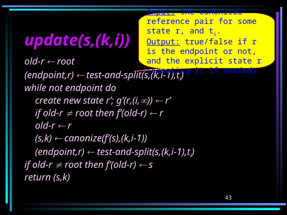
update(s,(k,i))update(s,(k,i))old-r root(endpoint,r) test-and-split(s,(k,i-1),ti)while not endpoint do

create new state r’; g’(r,(i,)) r’if old-r root then f’(old-r) rold-r r(s,k) canonize(f’(s),(k,i-1))(endpoint,r) test-and-split(s,(k,i-1),ti)

if old-r root then f’(old-r) sreturn (s,k)

Input: the canonical reference pair for some state r, and ti.Output: true/false if r is the endpoint or not, and the explicit state r (creating it if needed).

44

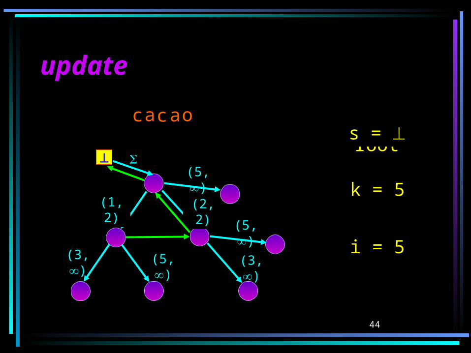
(2,)(2,2)

(1,)(1,2)

updateupdate

(3,)(3,)

(5,)

(5,)

(5,)

c ocaa s = root

k = 1

i = 1

s = s = root

k = 2

i = 2

s = s = root

k = 3

i = 3i = 4i = 5

k = 4k = 5

s =

45

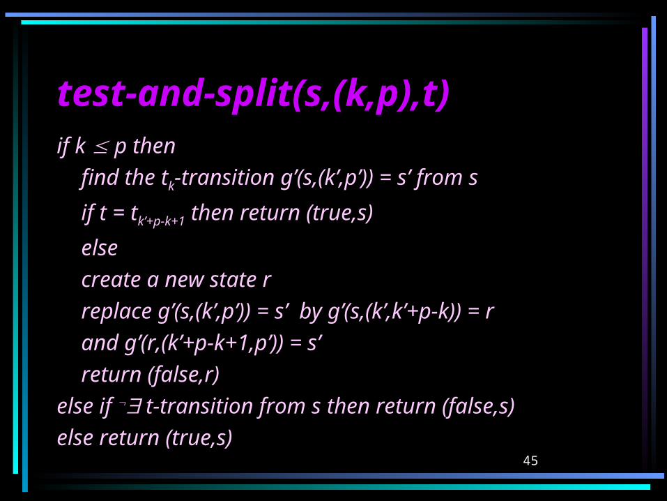
test-and-split(s,(k,p),t)test-and-split(s,(k,p),t)if k p then

find the tk-transition g’(s,(k’,p’)) = s’ from s

if t = tk’+p-k+1 then return (true,s)

elsecreate a new state rreplace g’(s,(k’,p’)) = s’ by g’(s,(k’,k’+p-k))

= rand g’(r,(k’+p-k+1,p’)) = s’

return (false,r)else if t-transition from s then return (false,s)else return (true,s)

46

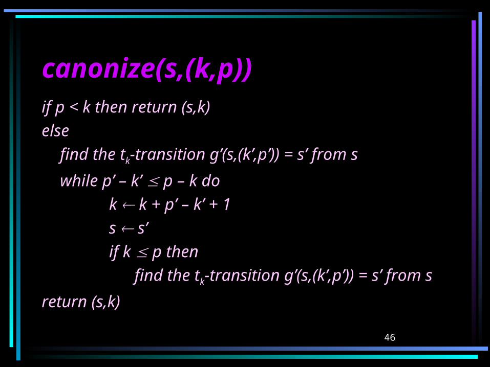
canonize(s,(k,p))canonize(s,(k,p))if p < k then return (s,k)else

find the tk-transition g’(s,(k’,p’)) = s’ from s

while p’ – k’ p – k dok k + p’ – k’ + 1s s’if k p then find the tk-transition g’(s,(k’,p’)) = s’

from sreturn (s,k)

47

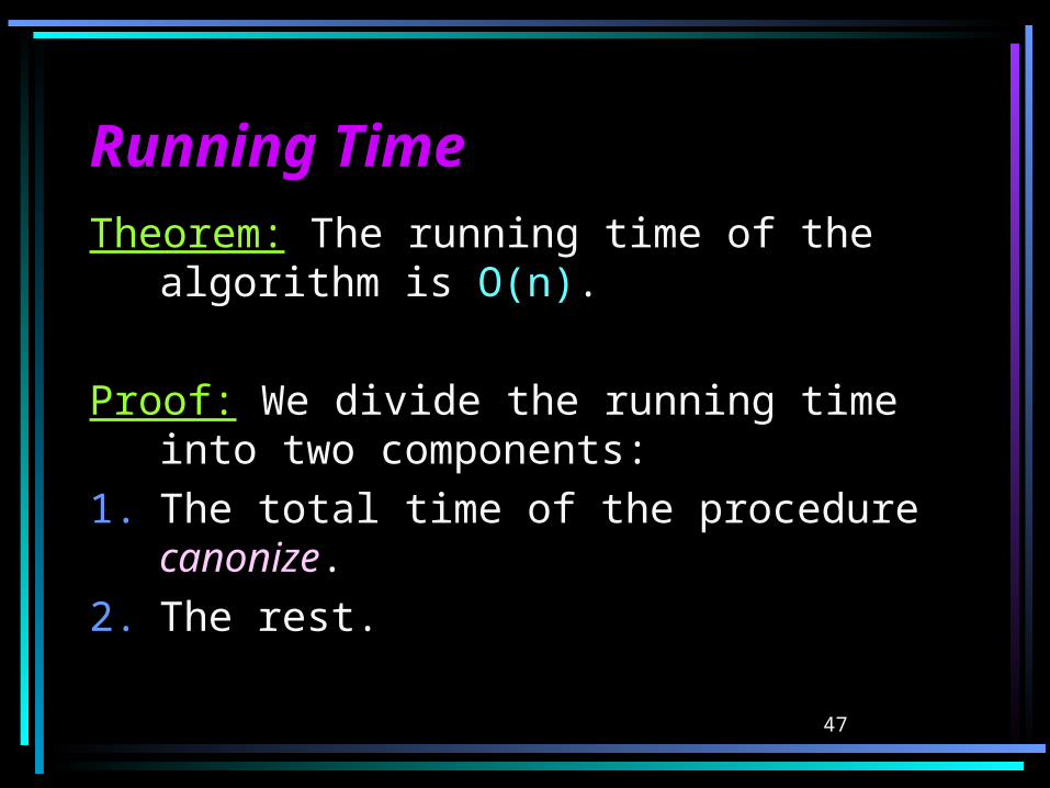
Running TimeRunning TimeTheorem: The running time of the

algorithm is O(n).

Proof: We divide the running time into two components:

1. The total time of the procedure canonize.

2. The rest.

48

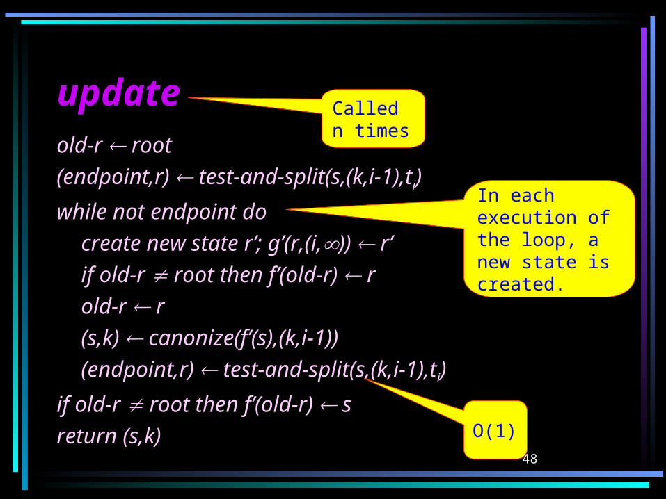
updateupdateold-r root(endpoint,r) test-and-split(s,(k,i-1),ti)

while not endpoint docreate new state r’; g’(r,(i,)) r’if old-r root then f’(old-r) rold-r r(s,k) canonize(f’(s),(k,i-1))(endpoint,r) test-and-split(s,(k,i-1),ti)

if old-r root then f’(old-r) sreturn (s,k)

In each execution of the loop, a new state is created.

O(1)

Called n times

49

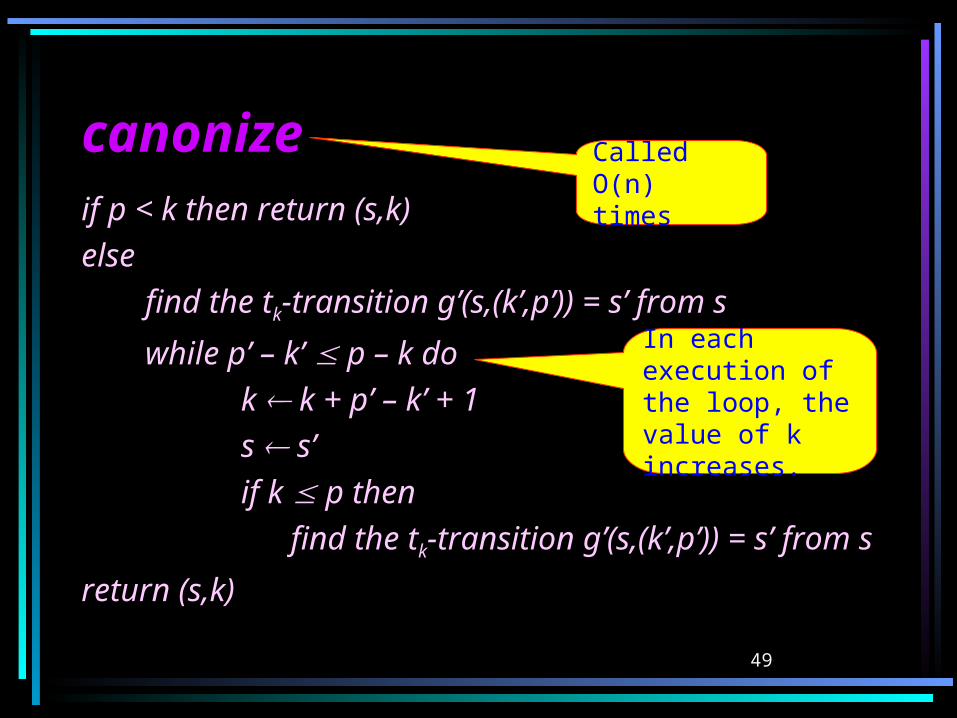
canonizecanonizeif p < k then return (s,k)else

find the tk-transition g’(s,(k’,p’)) = s’ from s

while p’ – k’ p – k dok k + p’ – k’ + 1s s’if k p then find the tk-transition g’(s,(k’,p’)) = s’

from sreturn (s,k)

In each execution of the loop, the value of k increases.

Called O(n) times

50

Applications - Exact String Applications - Exact String MatchingMatchingInput: two strings: a text T and a pattern

P.

Output: all the occurrences of P in T.

This problem can be solved in O(|T|+|P|) time (Boyer-Moore, Knuth-Morris-Pratt).

51

Applications - Exact String Applications - Exact String Matching (cont.)Matching (cont.) We look at the case where we have a

text T first, and then a sequence of patterns P1,…,Pr.

This problem can be solved using suffix trees.

Preprocessing time: O(|T|). Finding a pattern P: O(|P|+k), where k is

the number of occurrences of P in T.

52

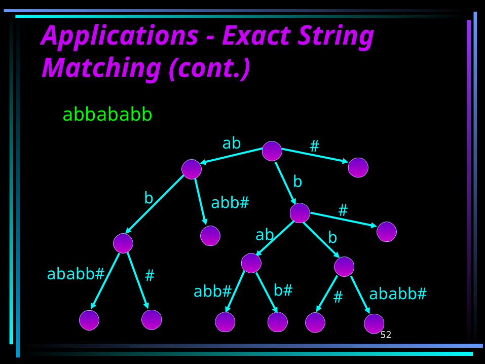
Applications - Exact String Applications - Exact String Matching (cont.)Matching (cont.)

abbababb

#ababb#

bb

ab

abb#

ab b

abb# b#

#

ababb#

#

#

53

Applications in BiologyApplications in Biology

54

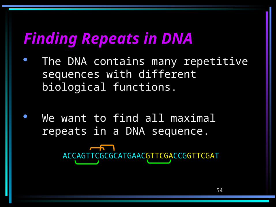
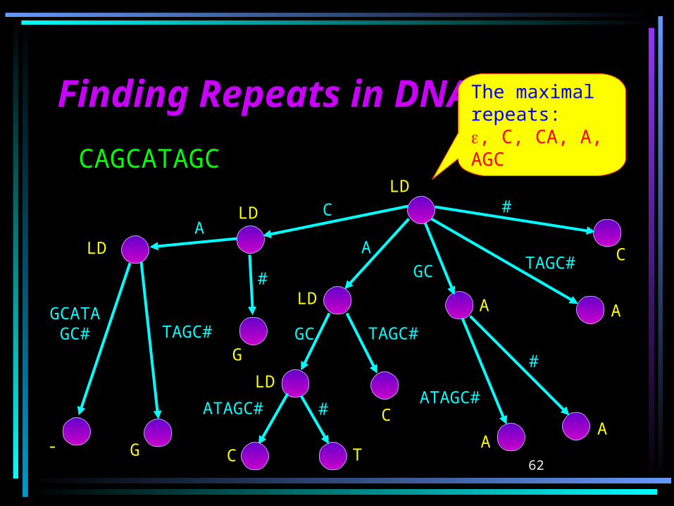
Finding Repeats in DNAFinding Repeats in DNA The DNA contains many repetitive

sequences with different biological functions.

We want to find all maximal repeats in a DNA sequence.

ACCAGTTCGCGCATGAACGTTCGACCGGTTCGAT

55

Finding Repeats in DNA Finding Repeats in DNA (cont.)(cont.)Theorem: All maximal repeats in a

sequence T can be found in O(|T|) time using suffix trees.

56

Finding Repeats in DNA Finding Repeats in DNA (cont.)(cont.)Lemma: If w is a maximal repeat in T,

then the state w in STree(T) is explicit.

Proof: If w is a maximal repeat then there are at least two occurrences of w in T s.t. the character following w is different. Thus w is a branching state, and therefore it is explicit.

57

Finding Repeats in DNA Finding Repeats in DNA (cont.)(cont.)Corollary: There are at most O(|T|)

maximal repeats in T.

Proof: By the above lemma, each maximal repeat corresponds to an explicit state. Since STree(T) has O(|T|) explicit states, T has O(|T|) maximal repeats.

58

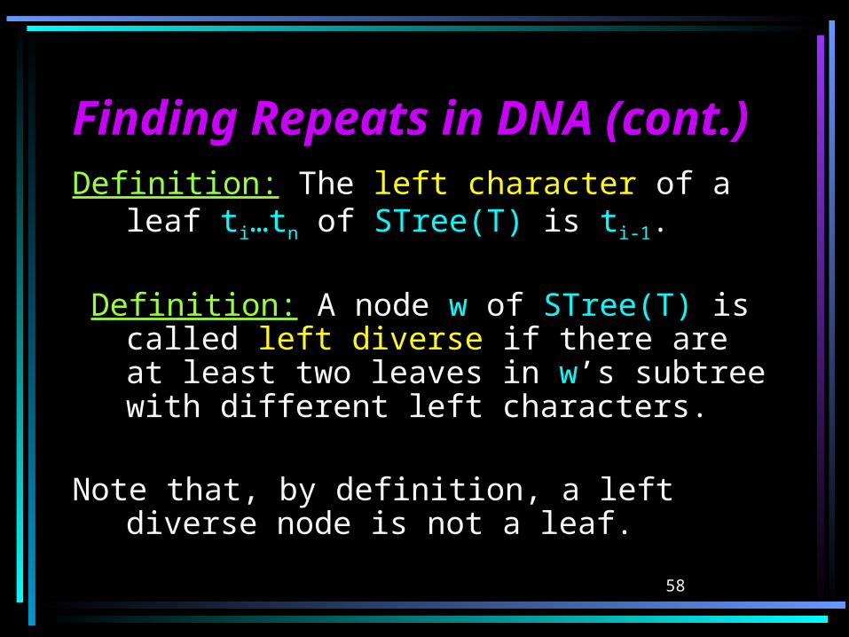
Finding Repeats in DNA Finding Repeats in DNA (cont.)(cont.)Definition: The left character of a leaf ti…tn

of STree(T) is ti-1.

Definition: A node w of STree(T) is called left diverse if there are at least two leaves in w’s subtree with different left characters.

Note that, by definition, a left diverse node is not a leaf.

59

Finding Repeats in DNA Finding Repeats in DNA (cont.)(cont.)Lemma: A substring w of T is a maximal

repeat iff w is a left diverse explicit state in STree(T).

60

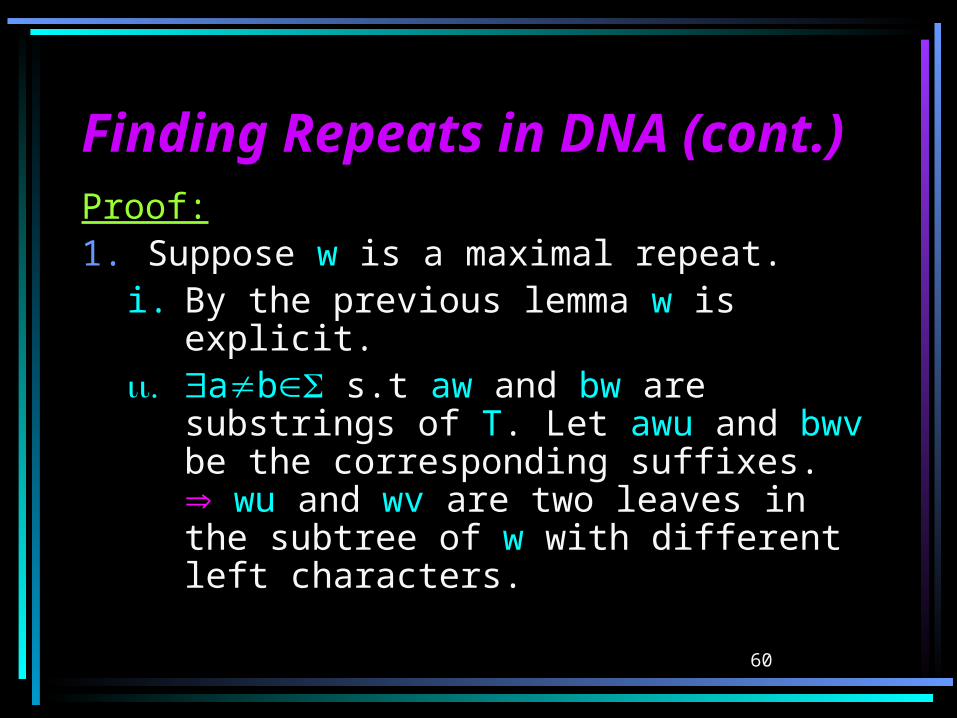
Finding Repeats in DNA Finding Repeats in DNA (cont.)(cont.)Proof:1. Suppose w is a maximal repeat.

i. By the previous lemma w is explicit.ii. ab s.t aw and bw are

substrings of T. Let awu and bwv be the corresponding suffixes. wu and wv are two leaves in the subtree of w with different left characters.

61

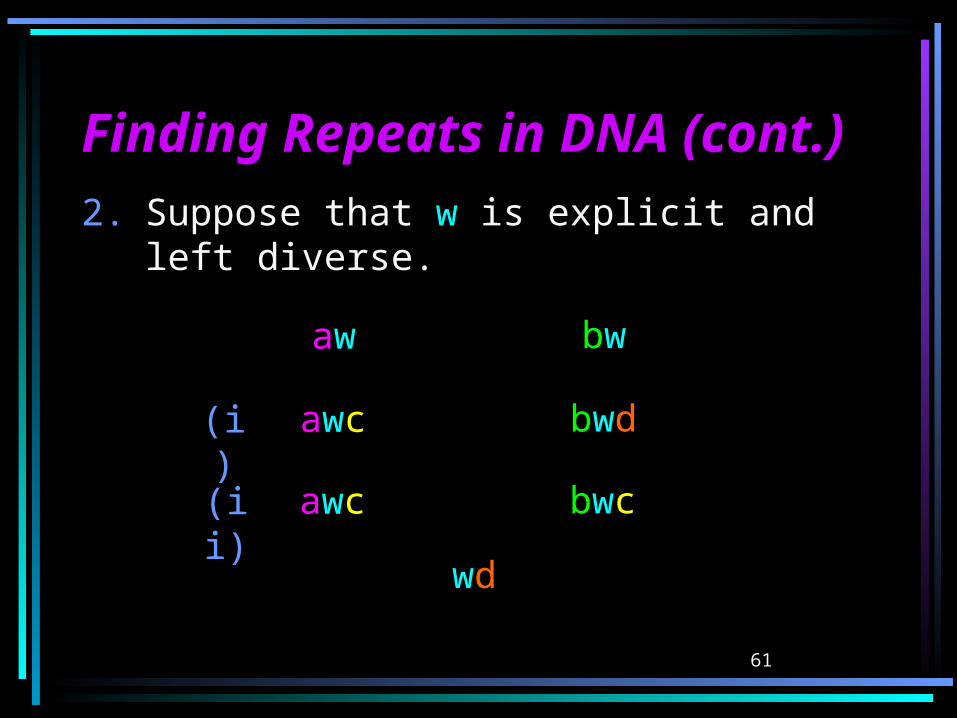
Finding Repeats in DNA Finding Repeats in DNA (cont.)(cont.)2. Suppose that w is explicit and left

diverse.

bwaw

bwdawc(i)

bwcawc(ii)

wd

62

Finding Repeats in DNA Finding Repeats in DNA (cont.)(cont.)

TAGC#GCATAGC#

AA

C

#

GC

TAGC#

ATAGC# #

GC

ATAGC#

#

TAGC#

#

CAGCATAGC

- G

LD

G

C

LD

T

LD

C

LD

AA

A A

C

LD

The maximal repeats:, C, CA, A, AGC

63

BibliographyBibliography On-Line Construction of Suffix Trees

E. Ukkonen

Algorithms on String, Trees, and SequencesDan Gusfield