1

1

Optimization Design of Stabilizing Piles in Slopes Considering Spatial Variability 2

Wenping Gong1, Huiming Tang2, C. Hsein Juang3, and Lei Wang4 3

4 1 Professor, Faculty of Engineering, China University of Geosciences, Wuhan, Hubei 430074, 5

China. Email: wenpinggong@cug.edu.cn 6 2 Professor, Faculty of Engineering, China University of Geosciences, Wuhan, Hubei 430074, 7

China. Email: tanghm@cug.edu.cn 8 3 Chair Professor, Department of Civil Engineering and Graduate Institute of Applied 9

Geology, National Central University, Taoyuan City 32001, Taiwan; also affiliate with 10

Faculty of Engineering, China University of Geosciences, Wuhan, Hubei 430074, China, and 11

Clemson University, Clemson SC 29634, USA. Email: hsein@clemson.edu 12 4 Assistant Professor, Department of Civil Engineering, University of the District of Columbia, 13

Washington, DC 20008, USA. Email: lei.wang@udc.edu (Corresponding author) 14

15

Abstract: Although advances in piling equipment and technologies have extended the global 16

use of stabilizing piles (to stabilize slope or landslide), the design of stabilizing piles remains 17

a challenge. Specifically, the installation of stabilizing piles can alter the behavior of the slope; 18

and, the spatial variability of the geotechnical parameters required in the design is difficult to 19

characterize with certainty, which can degrade the design performance. This paper presents an 20

optimization-based design framework for stabilizing piles. The authors explicitly consider the 21

coupling between the stabilizing piles and the slope, and the robustness of the stability of the 22

reinforced slope against the spatial variability of the geotechnical parameters. The proposed 23

design framework is implemented as a multi-objective optimization problem considering the 24

design robustness as an objective, in addition to safety and cost efficiency, two objectives 25

considered in the conventional design approaches. The design of stabilizing piles in an earth 26

slope is studied as an example to illustrate the effectiveness of this new design framework. A 27

comparison study is also undertaken to demonstrate the superiority of this new framework 28

over the conventional design approaches. 29

2

30

Keywords: Stabilizing Piles; Slope; Factor of Safety; Design Robustness; Spatial Variability; 31

Multi-Objective Optimization. 32

33

3

1. Introduction 34

“Stabilizing piles” are the piles that are installed to stabilize unstable slopes or active 35

landslides, which transfer part of the earth pressure from the upper unstable layer to the lower 36

stable layer, thus improving the stability of the geomaterials behind the piles (Poulos 1995; 37

Zeng and Liang 2002; Lirer 2012). Since their inception, stabilizing piles have been widely 38

used in the mitigation of slope instability and landslide geohazards. For example, many active 39

landslides and unstable slopes in the Three Gorges Reservoir Area have been reinforced with 40

stabilizing piles (Tang et al. 2014&2019). It is known that the installation of stabilizing piles 41

can greatly alter the behavior of the slope. The stability of a reinforced slope could be 42

evaluated with both uncoupled and coupled methods. In an uncoupled analysis, the earth 43

pressure and its distribution along the piles are first estimated, followed by the use of the earth 44

pressure as an input to the analysis of the behavior of the pile-slope system (Ito and Matsui 45

1975; Galli and Di Prisco 2012); whereas, in a coupled analysis, the piles and the slope are 46

dealt as an integrated system, and the behavior of this system is studied considering explicitly 47

the pile-slope interaction (Jeong et al. 2013). Though theoretically sound, the computationally 48

demanding characteristics of this coupled analysis might hinder its application in engineering 49

practice. As a result, the uncoupled analysis still dominates the design of stabilizing piles in 50

the current practice. 51

Though the behavior of the pile-slope system has been the subject of extensive studies, 52

little effort has been undertaken to elucidate design methods for stabilizing piles, especially 53

on the selection of pile parameters such as the diameter, spacing, length and position (Lee et 54

al. 1995). Indeed, the design of stabilizing piles is a multidisciplinary problem, which must be 55

informed with knowledge of geotechnical engineering, structural engineering, and economics. 56

4

Hence, the design of the stabilizing piles would better be implemented as a multi-objective 57

optimization problem, in which the requirements from the stability of the reinforced slope, 58

bearing capacity of the piles, and economic concerns should be simultaneously considered. 59

However, most of the discussions regarding the design of stabilizing piles do not encompass 60

economic requirements but instead place most emphasis upon either the stability of reinforced 61

slope or the pile bearing capacity (Chen and Martin 2002; Comodromos et al. 2009). 62

The geomaterials (e.g., soils and/or rocks) within a slope are natural materials, and the 63

properties of the geomaterials are dependent upon the natural deposit and loading histories, 64

which are beyond the control of the engineer. Due to the incomplete knowledge regarding the 65

deposit and loading histories, the geotechnical properties at a site could not be known prior to 66

the site investigation. In addition, because only a limited number of boreholes are afforded in 67

a given project, the geotechnical properties are only known at the borehole locations. The 68

properties at all other positions cannot be known and must be characterized from the known 69

values at the borehole locations. Owing to the inherent spatial variability of the geotechnical 70

properties and the limited availability of borehole data, the geotechnical properties at a given 71

site will be uncertain. The uncertain geotechnical properties are often characterized with fuzzy 72

or random variables, or random fields (Cho 2007; Wang et al. 2010; Ching and Phoon 2013; 73

Tian et al. 2016; Xiao et al. 2016; Li et al. 2017; Wang et al. 2017; Xiao et al. 2017; Zhang et 74

al. 2017; Liu and Cheng 2018; Kawa and Puła 2019; Tun et al. 2019). The uncertainty in the 75

input geotechnical properties further complicates the design of stabilizing piles. 76

In the face of the geotechnical properties uncertainty, the level of stability of a slope, 77

regardless of whether it is reinforced with stabilizing piles or not, will be uncertain and could 78

not be expressed as a fixed value (Griffiths and Fenton 2004; Cho 2007; Li et al. 2016; Wang 79

5

et al. 2018). To compensate for this uncertainty, a conservative estimate of the geotechnical 80

properties is usually made in the design. And, to further ensure safety, the computed factor of 81

safety FS, as a measure of the safety level, in a feasible design is required to be no less than a 82

target FS. With such a deterministic design approach, however, the true safety of a candidate 83

design is unknown, the resulting design might be either over- or under-designed. Alternatively, 84

the probabilistic design approaches that allow for an explicit consideration of the uncertainty 85

have long been advocated (Li and Lumb 1987; Christian et al. 1994; Duncan 2000; Juang et al. 86

2018). However, the designs obtained with the probabilistic approaches are strongly affected 87

by the statistical information of the input geotechnical properties (Wang et al. 2013; Juang et 88

al. 2014), which are difficult to characterize. Thus, the dilemma of whether to over-design for 89

safety or under-design for cost efficiency has not been fully overcome, even though the design 90

approaches evolve from deterministic to probabilistic approaches. To address this dilemma, 91

robust design methods, originated in the field of quality and industrial engineering (Taguchi 92

1986; Phadke 1989; Beyer and Sendhoff 2007), have recently been adopted for applications in 93

geotechnical designs (Juang and Wang 2013; Juang et al. 2014; Khoshnevisan et al. 2014). In 94

the context of robust geotechnical design (RGD), the design robustness of the geotechnical 95

system against the uncertainty in the input geotechnical parameters is explicitly considered 96

along with cost and safety requirements. 97

In this paper, a new framework for the robust design of stabilizing piles is established 98

that considers: 1) the coupling between the stabilizing piles and the slope; 2) the robustness of 99

the stability of the reinforced slope against the uncertainty in the input parameters; and 3) the 100

multi-objective optimization of the design robustness, economic aspect, and safety. The rest 101

of this paper is organized as follows. First, this new optimization-based design framework for 102

6

stabilizing piles is established. A hypothetical example, in terms of the design of stabilizing 103

piles in a homogeneous earth slope, that utilizes this new design framework is then detailed. 104

Thereafter, a comparison with the conventional geotechnical design approaches is undertaken 105

to demonstrate the superiority of the advanced framework. Finally, the concluding remarks 106

are made based upon the results presented. 107

108

2. New Design Framework for Stabilizing Piles in Slopes 109

While the significance of the coupling between the stabilizing piles and the slope, the 110

uncertainty in the input geotechnical parameters, and the economic constraint in the design of 111

stabilizing piles have long been recognized, an integrated design framework that can consider 112

explicitly all these factors remains unavailable. In this paper, a new optimization-based design 113

framework for stabilizing piles that considers all these factors simultaneously is advanced. 114

2.1 Modeling of the coupling in the pile-slope system 115

Figure 1 illustrates the coupling in a pile-slope system, in which the failure surface in 116

an unreinforced slope and those in reinforced slopes (with three designs of stabilizing piles 117

herein) are examined. In Figure 1(a), the depth of the failure surface in the unreinforced slope 118

is shallow and passes above the slope toe. In Figure 1(b) and Figure 1(c), the piles are located 119

around the middle part of the slope, and the pile lengths are greater than the depth of the 120

initial failure surface; as a result, the failure surfaces in the reinforced slopes extend to greater 121

depths. However, the length of the piles in Figure 1(b) is only slightly greater than the depth 122

of the initial failure surface, unlike the one in Figure 1(c). Consequently, the failure surface in 123

the reinforced slope in Figure 1(b) could not be blocked by the piles; and, the earth pressure 124

transferred by the piles, indicated by the maximum bending moment of the piles Mmax, is quite 125

7

small (i.e., Mmax = 99.4 kNm), indicating that the bearing capacity of the piles cannot be fully 126

utilized. On the other hand, the failure surface in the reinforced slope in Figure 1(c) could be 127

blocked by the piles, and a greater part of the earth pressure from the upper unstable layer is 128

transferred to the lower stable layer (i.e., Mmax = 1153 kNm). Thus, the improvement of the 129

slope stability, indicated by the factor of safety of the reinforced slope FS2, in Figure 1(c) is 130

more significant (i.e., FS2 = 1.28) than that in Figure 1(b) (i.e., FS2 = 1.09). In Figure 1(d), the 131

stabilizing piles are located in the lower part of the slope and the length of the piles is much 132

greater than the depth of the initial failure surface, which causes a reduction in the length of 133

the failure surface in the reinforced slope, and the new failure surface passes above the top of 134

the piles. Note that although the earth pressure transferred by the piles is significant in Figure 135

1(d) (i.e., Mmax = 1081 kNm), the improvement of the slope stability is not apparent (i.e., FS2 136

= 1.16). Thus, the failure surface, earth pressures on piles, and stability of reinforced slope are 137

all affected by the coupling between the stabilizing piles and the slope. This coupling must be 138

explicitly considered in the analysis and design of stabilizing piles. 139

Given the recognized effectiveness of numerical solutions for analyzing the coupling 140

between the structures and the geomaterials, the 2-D explicit finite difference program FLAC 141

version 7.0 (2011) is adopted herein as the solution model for evaluating the stability of the 142

pile-slope system. Within FLAC version 7.0, the slope stability is evaluated with the strength 143

reduction method, in which the resistance (i.e., shear strength) of the geomaterials is gradually 144

adjusted to bring the slope (either reinforced or unreinforced) to the limit equilibrium state. It 145

is well known that the behavior of a pile-slope system is a 3-D problem and which should be 146

studied with 3-D numerical simulations; otherwise, the sliding of the geomaterials through the 147

space between adjacent piles could not be simulated. However, the 3-D numerical simulation 148

8

can be computationally prohibitive for the following probabilistic stability analysis and design 149

optimization. In reference to Kourkoulis et al. (2010), an effective soil arching can be formed 150

between adjacent piles when the ratio of the pile spacing over the pile diameter is less than 4.0. 151

Under such circumstances, the plane-strain condition is taken in this study and the maximum 152

ratio of the pile spacing (i.e., center-to-center spacing between piles) over the pile diameter is 153

set to be 3.0. Thus, the stability of the pile-slope system can be evaluated with 2-D numerical 154

simulations; in which, the piles are modeled with elastic-perfectly plastic beam elements, the 155

interfaces between the piles and the geomaterials are modeled with interface elements, and the 156

pile spacing is inputted to the numerical models to realize the resistance of the piles (against 157

slope failure) per longitudinal length. The plastic moment of the piles, which is required in the 158

2-D numerical simulations, is derived with plasticity theory of reinforced concrete. Since the 159

stability of a slope (either reinforced or unreinforced) can be dominated by the shear strength 160

of the geomaterials, the behaviors of the geomaterials in this study are simulated with Mohr-161

Coulomb models. 162

2.2 Formulation of the design robustness of the reinforced slope 163

For the pile-slope system with the design parameters d and the non-design variables 164

as inputs, the response or performance of this system g(d, θ) is expressed as: 165

( , ) ( , ) ( , )= −d d dg R T (1) 166

where R(d, θ) and T(d, θ) are the resistance term and load term, respectively. Mathematically, 167

the uncertainty in the input parameters will lead to the uncertainty in the output or system 168

response g(d, θ). In reference to Figure 2, the relationship between the output g(d, θ) and the 169

inputs is captured by a monotonic performance function g(d, θ). For an arbitrary distribution 170

of the inputs , the output g(d, θ) is a distribution, rather than a fixed value. 171

9

In a deterministic design, the safety of a design is evaluated and expressed as a factor 172

of safety FS: 173

( , )

( , )=

d

d

RFS

T

(2) 174

In practice, a design is deemed feasible if the computed FS is greater than 1.0. To compensate 175

for the uncertainty in the input parameters and adopted model, a conservative estimate of the 176

input parameters (e.g., 20th percentile of the resistance term R and 80th percentile of the load 177

term T; see Figure 2) and a target FS, FST (e.g., FST = a value greater than 1.0, say, 1.2), may 178

be adopted. Since the uncertainty is not explicitly included in the analysis, the true safety of 179

the design is unknown and the resulting design might be either over- or under-designed. To 180

overcome this problem, the probabilistic approaches which permit an explicit consideration of 181

the uncertainty (e.g., uncertain variables are simulated as random variables or random fields) 182

have long been advocated (Li and Lumb 1987; Christian et al. 1994; Cherubini 2000; Duncan 183

2000). In probabilistic designs, the safety of a design d is evaluated with the computed failure 184

probability Pf or reliability index . 185

0

-( , ) 0

Pr[ ( , ) 0] ( ) = ( )f

g

P g f d f g dg

= = d

d

(3a) 186

( )fP = − (3b) 187

where f() is the probability density function (PDF) of the uncertain input parameters ; f(g) is 188

the PDF of the performance function g(d, θ); and, () is the cumulative distribution function 189

(CDF) of the standard normal variable. To ensure the safety of the resulting design, a target 190

failure probability PfT (e.g., PfT = 4.710-3) or a target reliability index T (e.g., T = 2.6) is 191

suggested. A design is deemed feasible if the computed failure probability Pf is less than the 192

10

target failure probability PfT or the related reliability index is larger than the target reliability 193

index T. 194

Note that while the formulation is simple and easy-to-follow, the practical application 195

of the probabilistic approaches in the geotechnical design is not an easy task. The challenge in 196

the geotechnical design is attributed to the fact that the geomaterials are natural, rather than 197

manufactured materials. The degree of uncertainty in the geotechnical properties tends to be 198

greater than that in the structural counterpart and the uncertainty in the geotechnical properties 199

could be much more difficult to characterize. Furthermore, the property of the geomaterials is 200

often spatially correlated. The spatial correlation characteristics of the geotechnical properties 201

could best be characterized with the random field theory (Fenton 1999; Cho 2007; Tian et al. 202

2016). The anisotropic exponential autocorrelation structure is adopted herein to capture the 203

spatial correlation of the geotechnical properties: 204

( ) 1 2 1 2

1 2 1 2

h v

2 2, exp exp

x x y yx x y y

− − − − = − −

(4) 205

where |x1 – x2| is the horizontal distance between the two positions of (x1, y1) and (x2, y2); |y1 – 206

y2| is the vertical distance between the two positions of (x1, y1) and (x2, y2); and, h and v are 207

the horizontal and vertical scale of fluctuations of the geotechnical properties, respectively. 208

In a numerical modeling of a slope (either reinforced or unreinforced), the geometrical 209

domain of the slope is discretized into a set of small elements, thus permitting an assignment 210

of different geotechnical properties to different numerical elements. That is to say, the spatial 211

variability of the geotechnical parameters can be directly simulated in the numerical modeling. 212

Note that while lots of computationally efficient methods have been developed for the 213

probabilistic analysis of the geotechnical systems, most of them cannot be applied to 214

11

geotechnical systems with random fields as inputs; whereas, the sampling-based methods 215

such as the Monte Carlo simulation (MCS) are often deemed the most reliable approaches for 216

dealing with the random fields. To consider the spatial variability of the input geotechnical 217

parameters in the design of stabilizing piles, the random finite difference method (RFDM) is 218

adopted in this study. In the context of the RFDM, the spatial variability of the input 219

geotechnical parameters is simulated with the random field theory, and potential realizations 220

of the random field of the geotechnical parameters are sampled with MCSs. For each and 221

every realization of the random field, the stability of the slope will be analyzed 222

deterministically utilizing the finite difference program (e.g., the 2-D FLAC adopted in this 223

paper). Since the parameters within a numerical element are captured by fixed parameters and 224

no variation can be allowed, the geotechnical parameters that are averaged within the element 225

domain, rather than those at the grids, should be sampled and taken as the inputs to the 226

numerical analysis. The integration of brute MCS and numerical analysis can be 227

computationally prohibitive. To improve the computational efficiency (of this RFDM), the 228

subdomain sampling method (SSM) (Juang et al. 2017), in lieu of the brute MCS, is adopted 229

in this paper for sampling the potential realizations of the random field of the input 230

geotechnical parameters. A detailed formulation of this SSM is summarized in Appendix A. 231

In a typical geotechnical practice, site-specific data can be quite limited due to budget 232

constraints for site investigation. Thus, it is difficult to derive the statistical information of the 233

input geotechnical parameters with certainty (Gong et al. 2017). In such a circumstance, the 234

probabilistic approaches are usually undertaken using inaccurate or assumed statistics; 235

however, the designs obtained with the probabilistic approaches are strongly influenced by the 236

adopted statistics (Wang et al. 2013). To overcome this issue of the probabilistic approaches, 237

12

robust design, originated from the field of quality and industrial engineering (Taguchi 1986), 238

is adopted, in this paper, for the design of stabilizing piles. The essence of this robust design 239

is to derive a design in which the system behavior is robust against the uncertainty in the input 240

parameters. In the proposed robust design of stabilizing piles, the robustness of the stability of 241

the reinforced slope against the uncertainty (i.e., spatial variability) in the input geotechnical 242

parameters, R, is formulated based upon the concept of “signal-to-noise ratio” (SNR) (Phadke 243

1989; Gong et al. 2014a). 244

2

210 2

2

[ ]10 log

[ ]

E FSR SNR

FS

= =

(5) 245

where E[FS2] and [FS2] are the mean and standard deviation, respectively, of the stability of 246

the reinforced slope. Note that although various robustness measures have been developed for 247

the robust geotechnical design (RGD) (Wang et al. 2013; Juang et al. 2014; Khoshnevisan et 248

al. 2014; Gong et al. 2014a&2014b), the selection of the robustness measure can be problem-249

specific depending upon the level of uncertainty in geotechnical parameters characterization: 250

1) in the scenario where only the nominal values of the geotechnical parameters are known, 251

the gradient-based robustness may be utilized (Gong et al. 2014b); 2) in the scenario where 252

the ranges of the geotechnical parameters could be estimated, the SNR-based robustness may 253

be utilized (Gong et al. 2014a); and 3) in the scenario where the probabilistic distribution of 254

the geotechnical parameters may be characterized but the statistical information could not be 255

ascertained, the feasibility-based robustness may be used (Wang et al. 2013). In the proposed 256

robust design of stabilizing piles, the noise factors (i.e., difficult-to-characterize and hard-to-257

control parameters) are mainly associated with the spatially varied geotechnical parameters. 258

Note that while the feasibility-based robustness is theoretically sound, the simpler SNR-based 259

13

robustness measure formulated in Eq. (5) is adopted herein owing to its simplicity and 260

practical applicability. As such, the calculation of the feasibility of the failure probability 261

satisfying the target failure probability can be avoided; meanwhile, the characterization of the 262

uncertainty in the statistical parameters of the geotechnical properties, which is required for 263

the feasibility calculation, can be avoided. 264

With the numerical model established in the previous section as a solution model, the 265

uncertainty in the noise factors naturally propagates into the uncertainty in the stability of the 266

reinforced slope, which could be captured by the standard deviation of the stability (in terms 267

of the factor of safety FS) of the reinforced slope [FS2]. It is noted that a higher [FS2] value 268

indicates a higher variability of the stability of the reinforced slope (in the face of the input 269

geotechnical properties uncertainty), thus signaling a lower robustness of the stabilizing pile 270

design. Since the safety of the stabilizing pile design can also be affected by the mean of the 271

stability of the reinforced slope E[FS2], the standard deviation of the stability [FS2] is further 272

normalized by the mean of the stability E[FS2]. Then, the SNR-based robustness R is readily 273

formulated, as shown in Eq. (5). Similarly, a higher R value signals a lower variability of the 274

stability of the reinforced slope, and thus indicating a higher robustness. Here, the detailed 275

procedure for derivation of the mean E[FS2] and standard deviation [FS2] of the stability of 276

the reinforced slope using the subdomain sampling method (SSM) is given in Appendix A. In 277

reference to the robustness measure formulated in Eq. (5), the conventional factor of safety FS 278

is embedded in this design robustness; and, this design robustness measure is calculated from 279

the by-products of the probabilistic analysis, in terms of the statistics of the factor of safety FS. 280

Hence, the proposed design framework is compatible with the conventional deterministic and 281

probabilistic design approaches; and, the computational coupling of the evaluation of the 282

14

design robustness and the probabilistic analysis would not lead to significant increase in the 283

computational demands of the advanced robust design. Indeed, the only increase in the 284

computational demand of the advanced design framework is the multi-optimization shown in 285

Eq. (6), in comparison to the conventional probabilistic design approaches. 286

2.3 Optimization-based design of stabilizing piles incorporating robustness 287

The goal of the advanced optimization-based design framework for stabilizing piles is 288

to derive an optimal stabilizing pile design (represented by a set of design parameters d) in the 289

design space DS such that the target stability of the reinforced slope TS can be satisfied, while 290

both robustness R and cost efficiency E will be simultaneously optimized. This optimization-291

based design framework for stabilizing piles is set up as follows. 292

ult

Find: Pile parameters

Subject to: Design space

Target stability of

Ultimate bearing cap

reinforced slope

acity of stabilizi ng pile

Objectiv

s M

d

DS

TS

es: Maximizing design robustness

Minimizing constru ctio n c ost

R

C

(6) 293

where d represents the design parameters of the stabilizing piles that are easy-to-control (by 294

the engineer). For example, the geometrical parameters of the pile diameter D, pile spacing S, 295

pile length L and pile position X are taken as the design parameters d, expressed as d = {D, S, 296

L, X}. Whereas, the mechanical parameters of the piles such as the steel reinforcement ratio 297

and concrete modulus are taken as fixed values; and, the steel strength and concrete strength, 298

which are essential for estimating the ultimate bearing capacity of the piles, could be dealt as 299

uncertain parameters (or noise factors) due to the manufacturing error. 300

The design space DS is an assembly of candidate designs of stabilizing piles, which 301

can be determined based upon local experience and engineering judgment. The target stability 302

15

TS is a mandatory requirement of the stability of the reinforced slope, expressed in terms of 303

the target factor of safety FST or target failure probability PfT (or equivalently target reliability 304

index T), which could be specified by the owner or client based upon the significance of the 305

project or consequences of failure. The ultimate bearing capacity Mult is the plastic moment of 306

the piles, which is evaluated with the plasticity theory of steel reinforced concrete. The design 307

robustness R is the “signal-to-noise ratio” (SNR) of the stability of the reinforced slope against 308

the variation in the uncertain input parameters (or noise factors). The construction cost C is 309

the economic aspect of the design of stabilizing piles. Assuming no variation in the cost with 310

respect to the site condition and pile installation technique in a given project, only the material 311

cost of the piles is considered in this paper. Further, the steel reinforcement ratio of the piles is 312

taken as a fixed value. Thus, the cost C could be approximated herein by the volume of the 313

stabilizing piles per longitudinal length. 314

2

04

D LC C

S

=

(7) 315

where C0 represents the cost per cubic meter of steel reinforcement concrete. 316

The desire to maximize the design robustness R and that to minimize the cost C are 317

two conflicting objectives. The optimization in Eq. (6) cannot lead to a single best design with 318

respect to both objectives simultaneously. Instead, this optimization only leads to a set of non-319

dominated designs which are superior to all others in the design space, but not superior or 320

inferior to any other in this set. As depicted in Figure 3, although the non-dominated design d1 321

is less expensive (indicating higher cost efficiency), the counterpart of non-dominated design 322

d2 yields a larger R value (indicating higher robustness). Note that although the utopia design 323

d0 is optimal with respect to both objectives, it may not be located in the feasible domain (i.e., 324

16

the target stability TS is not satisfied or not belong to design space DS). These non-dominated 325

designs collectively form a Pareto front which reveals a tradeoff relationship between these 326

two conflicting design objectives (Deb et al. 2002; Juang et al. 2014). This Pareto front can be 327

obtained utilizing multi-objective optimization algorithms such as the Multi-objective Genetic 328

Algorithm, MOGA (Murata and Ishibuchi 1995), Niched Pareto Genetic Algorithm, NPGA 329

(Horn et al. 1994), Non-dominated Sorting Genetic Algorithm version II, NSGA-II (Deb et al. 330

2002; Juang and Wang 2013), Multi-algorithm Genetically Adaptive Multiobjective Method, 331

AMALGAM (Vrugt and Robinson 2007; Huang et al. 2014), weighted sum-based algorithm 332

(Hajela and Lin 1992), or spreadsheet-based algorithm (Khoshnevisan et al. 2014). 333

Note that although various optimization algorithms could be available in the literature 334

of industrial, civil and electrical engineering, the optimization of the geotechnical system such 335

as the stabilizing piles is different from the optimization problem in other fields. For example, 336

the choice of the pile diameter is limited to piling equipment and local practice, only discrete 337

values can be taken. A survey of the geometrical parameters of the stabilizing piles installed 338

in the Three Gorges Reservoir Area, China indicates that the pile lengths were often taken as 339

discrete or integer values and the piles were usually constructed at the elevations of discrete or 340

integer values. Thus, a discrete design space DS is selected in this paper for the optimization 341

design of stabilizing piles to ensure the feasibility in the construction. Since a discrete design 342

space is adopted with a finite number of candidate designs (e.g., 480 designs in this paper), 343

the optimization presented in this study adopts an exhaustive search among the designs in the 344

discrete design space, which is different from many other optimization techniques reported in 345

the literature (e.g., Hajela and Lin 1992; Murata and Ishibuchi 1995; Deb et al. 2002; Vrugt 346

and Robinson 2007), where potential candidate designs are generated and analyzed selectively, 347

17

and not exhaustively. Here, the safety, robustness, and cost for each and every candidate 348

design in the selected discrete design space are evaluated. On the basis of the evaluated 349

performance of candidate designs, the Pareto front revealing the tradeoff between design 350

robustness and cost efficiency can be derived utilizing the non-dominated sorting algorithm in 351

the NSGA-II (Deb et al. 2002). It should be noted that although a discrete design space is 352

adopted in this study, it is not the limitation of the advanced design framework and a 353

continuous design space can also be adopted if so desired (and then the optimization 354

algorithms reported in the literature can be applied); however, the random finite difference 355

method (RFDM)-based probabilistic analysis of the candidate design will be iteratively called 356

in the direct application of these optimization algorithms, which might increase the 357

computational efforts for this problem. 358

The obtained Pareto front could help render an informed design decision. For example, 359

either the least cost design that is above a pre-specified level of robustness RP (see design d3 360

in Figure 3) or the most robust design that is below a pre-specified level of cost CP (see design 361

d4 in Figure 3) can be selected as the most preferred design in the design space DS. However, 362

the determination of an appropriate level of the robustness or cost is usually problem-specific. 363

In situations where a strong preference is not pre-specified by the owner or client, the knee 364

point on the Pareto front, which can yield the best compromise with respect to the conflicting 365

objectives, can be identified (see design d5 in Figure 3) and taken as the most preferred design 366

(Deb and Gupta 2011). As illustrated in Figure 3, on the left side of the knee point design d5, a 367

slight reduction in cost C could lead to a drastic decrease in the design robustness R, which is 368

not desirable; and, on the right side of the knee point design d5, a slight improvement in the 369

design robustness R requires a huge increase in cost C, which is also not desirable. Thus, this 370

18

knee point design could be taken as the most preferred design in the design pool, if no design 371

preference is specified by the owner or client. Once the Pareto front is obtained, this knee 372

point design is easily identified with the marginal utility function approach (Deb and Gupta 373

2011), normal boundary intersection approach (Deb and Gupta 2011), reflex angle approach 374

(Deb and Gupta 2011), or minimum distance approach (Gong et al. 2016a). 375

376

As can be seen, the coupling between the stabilizing piles and the slope, the robustness 377

of the stability of the reinforced slope against the uncertainty in the input parameters (e.g., the 378

spatial variability of the geotechnical parameters and the manufacturing error of the structural 379

materials), economic aspect, and conventional safety requirements are explicitly considered in 380

the advanced design framework for stabilizing piles; and, this design framework is carried out 381

through a multi-objective optimization with respect to these design objectives. 382

383

3. Illustrative Example: Design of Stabilizing Piles in An Earth Slope 384

To demonstrate the effectiveness and significance of the advanced design framework, 385

the design of stabilizing piles in a homogeneous earth slope, shown in Figure 4, is adopted as 386

an illustrative example. The parameters setting and the design results are presented below. 387

3.1 Parameters setting in the illustrative example 388

In reference to Figure 4, the width and height of the studied slope are 20.0 m and 14.0 389

m, respectively, and the depth to bed rock is assumed to approach infinity (H→ ). Further 390

assume no surcharge on the top of the slope and the groundwater level far below the slope. In 391

this example, both soil strength parameters, in terms of the cohesion c and friction angle , are 392

treated as random fields, and their statistical information is tabulated in Table 1. The other soil 393

19

parameters such as the unit weight, bulk modulus and shear modulus are assumed as fixed (or 394

deterministic) values, as listed in Table 2. 395

An initial analysis of this slope indicates that the stability of this slope is relatively low 396

(i.e., FS1 = 1.14), which is thus designed to be reinforced by a single row of steel reinforced 397

concrete stabilizing piles. According to the optimization framework outlined above, the easy-398

to-control geometrical parameters, including the pile diameter D, pile spacing S, pile length L 399

and pile position X, are taken as the design parameters d, expressed as d = {D, S, L, X}. The 400

steel reinforcement ratio and concrete modulus (of the piles) are treated as fixed values, as 401

shown in Table 2; and, the steel strength and concrete strength are taken as uncertain input 402

parameters and their statistical information is also given in Table 1. For ease of construction, a 403

discrete design space DS shown in Table 3 is selected in this paper for the optimization design. 404

The maximum ratio of the pile spacing S over the pile diameter D is set to be 3.0 (i.e., S/D = 405

3.0) in this optimization problem, thus effective soil arching can be formed between adjacent 406

piles (Kourkoulis et al. 2010). In the selected design space DS shown in Table 3, a total of 407

480 candidate designs are possible and the optimal design will be identified from this pool. 408

To incorporate the coupling between the stabilizing piles and the slope explicitly, the 409

numerical model established above is adopted herein as the solution model for evaluating the 410

safety performance of the pile-slope system. The 2-D explicit finite difference program FLAC 411

version 7.0 (2011) is used and plane-strain condition is assumed. To minimize the boundary 412

effect, the bottom boundary is set at 30.0 m below the slope toe, the left-side boundary is set 413

at 30.0 m away from the slope toe, and the right-side boundary is set at 30.0 m away from the 414

slope crest. The geometrical domain of this slope problem is discretized into 1,296 elements 415

(the minimum size of the discretized elements is 1.0 m×1.0 m) for ease of assigning the soil 416

20

parameters (e.g., c and ). The left- and right-side boundaries are restrained horizontally, and 417

the bottom boundary is restrained vertically. The soil is simulated with Mohr-Coulomb model, 418

the stabilizing piles are modeled with elastic-perfectly plastic beam elements, and the soil-pile 419

interfaces are modeled with interface elements. The setting of the parameters of the piles and 420

those of the interfaces is tabulated in Table 2. Note that a bracketing approach similar to that 421

proposed by Dawson et al (1999) is used in FLAC version 7 for deriving the factor of safety 422

FS of the slope, and the resolution limit is set at 0.02 in this paper. As such, the model error of 423

this numerical model, in terms of the discrepancy between the true FS and the calculated FS 424

(i.e., true FS minus calculated FS), might be taken as an uncertain variable that is uniformly 425

distributed in the range of [-0.02, 0.02]. 426

It should be noted that the execution of a deterministic analysis of the slope stability 427

takes about 100 seconds on the Windows 7® PC equipped with a 192 GB RAM and an Intel® 428

Xeon® Processor E5-2699 v4 @ 2.20 GHz. To reduce the number of the realizations or 429

samples of the uncertain input parameters involved in the RFDM analysis and thus improving 430

the computational efficiency, the subdomain sampling method (SSM) (Juang et al. 2017) is 431

utilized for generating the realizations of the random fields of soil strength parameters and the 432

samples of the other uncertain parameters (i.e., the steel strength, concrete strength and model 433

error). The parameters of the adopted SSM are set up as follows: 1) the probability of in Eq. 434

(A3) is taken as = 1.010-6 for locating the possible domain of uncertain parameters; 2) the 435

likelihoods of the samples being located in the subdomains are taken as a decreasing sequence 436

of pd1 = 1/3, pd2 = 1/32, pd3 = 1/33, … ; 3) the target number of samples in each subdomain is 437

taken as t1 = 30; and 4) the number of subdomains is taken as ns = 13. Thus, a total of 390 438

realizations or samples of the uncertain input parameters will be generated and analyzed for 439

21

estimating the statistics of the stability of the slope (either reinforced or unreinforced). This 440

number of samples is close to that required in the stochastic response surface method (Li et al. 441

2011&2015), which is well known for its high computational efficiency in analyzing random 442

field problems. 443

3.2 Results obtained with the advanced optimization-based design framework 444

With the derived statistics of the stability of the reinforced slope (using SSM), the 445

design robustness R, in terms of the “signal-to-noise ratio” (SNR), and the design safety, in 446

terms of the mean of the stability E[FS2] (to be compatible with the deterministic approach) or 447

failure probability Pf (to be compatible with the probabilistic approach) of the reinforced 448

slope, can readily be evaluated. For example, the failure probability of the reinforced slope Pf 449

(or equivalent reliability index ) in this paper is estimated with the fourth moment method 450

FM-1 outlined in Zhao and Ono (2001). Figure 5 validates the effectiveness and accuracy of 451

the adopted SSM, using MCS, in deriving the design robustness R, design safety E[FS2] and 452

design safety Pf of the reinforced slope through an analysis of 15 arbitrarily selected candidate 453

designs. Note that the number of samples utilized in the brute MCS herein is taken as 5,000. 454

In Figure 5(a) and Figure 5(b), the data points (of design robustness R and safety E[FS2]) are 455

both close to the 1:1 line (i.e., a perfect match), thus the design robustness R and design safety 456

E[FS2] estimated from the adopted SSM match well with those from the MCS. In Figure 5(c), 457

although there is some discrepancy in the derived failure probability Pf between the SSM and 458

the MCS, the 90% confidence interval of the failure probability Pf derived from the MCS can 459

bracket the failure probability Pf derived from the SSM with a high chance. In the context of 460

the brute MCS, the coefficient of variation of the failure probability estimate Pf, denoted as Pf, 461

is approximated as follows (Ang and Tang 2007). 462

22

1 f

Pf

MCS f

P

n P

−

(8) 463

where nMCS represents the number of samples utilized in the MCS. With the estimated failure 464

probability Pf and its COV, the 90% confidence interval of the failure probability Pf shown in 465

Figure 5(c) can readily be obtained with an assumption that the estimated failure probability 466

follows a lognormal distribution. From there, the accuracy of the adopted SSM in evaluating 467

the design robustness and safety of the reinforced slope is validated. However, with the SSM, 468

only 390 realizations (or samples) of the uncertain input parameters are required. As such, the 469

computational efficiency of the proposed optimization design could be guaranteed. 470

Since a discrete design space is adopted in this example, the design safety, robustness, 471

and cost for each and every candidate design could be evaluated and the results are shown in 472

Figure 6. The performance evaluation of these 480 candidate designs took approximately 30 473

days utilizing parallel computing on the Windows 7® PC equipped with a 192 GB RAM and 474

an Intel® Xeon® Processor E5-2699 v4 @ 2.20 GHz. To be compatible with the conventional 475

deterministic and probabilistic approaches, the design safety in this example is measured with 476

the mean of the stability E[FS2] and the reliability index (or equivalent failure probability Pf) 477

of the reinforced slope, respectively. Figure 6(a) depicts the relationship between the mean of 478

the stability E[FS2] and the cost C. Figure 6(b) depicts the relationship between the reliability 479

index and the cost C. Figure 6(c) depicts the relationship between the robustness R and the 480

cost C. In Figure 6(a) and Figure 6(b), the design safety tends to increase with the increase of 481

the cost C, as indicated by the increase of the mean of the stability E[FS2] and increase of the 482

reliability index . In Figure 6(c), the robustness also increases with the increase of the cost. 483

Thus, a more conservative and robust design will cost more, indicating that a tradeoff exists 484

23

between the safety (and robustness) and the cost. However, the various combinations of the 485

design parameters means that the candidate designs of similar cost level may yield different 486

levels of safety and robustness, and the candidate designs of different cost level may yield 487

similar level of safety and robustness. Indeed, these combinations of the design parameters 488

provide the theoretical basis for the optimization-based design of stabilizing piles. 489

In reference to the optimization algorithm of the stabilizing piles shown in Eq. (6), the 490

design of the stabilizing piles in this example slope is readily undertaken. Through the sorting 491

algorithm in the NSGA-II (Deb et al. 2002), a Pareto front consisting of nine non-dominated 492

designs is established in the selected design space DS, as depicted in Figure 6(c). This Pareto 493

front shows the tradeoff between the robustness and the cost. As can be seen from Figure 6(c), 494

these non-dominated designs on the Pareto front are superior to all others in the design space 495

(either costs less or yields higher design robustness). Next, the knee point on this Pareto front, 496

as depicted in Figure 6(c), is identified with the minimum distance approach outlined in Gong 497

et al. (2016a). Here, this knee point could be taken as the most preferred design in the design 498

space if the design constraint of the target stability TS is not applied. 499

It should be noted that the choice of the target stability TS can affect the resulting 500

design, as indicated by the design results obtained with different choices of the target stability 501

TS shown in Figure 7 and Table 4. The design results, in terms of the Pareto front and knee 502

point, obtained with two different levels of target FS (i.e., FST = 1.20 and 1.25) (MCPRC 503

2002) are illustrated in Figure 7(a) and Figure 7(b). Similarly, the design results obtained with 504

two different levels of target reliability index (i.e., T = 2.6 and 3.2) are shown in Figure 7(c) 505

and Figure 7(d). The design results in Figure 7 and Table 4 depict that a reduction in the target 506

stability TS, as reflected by the decrease of target factor of safety and the decrease of target 507

24

reliability index, could result in more feasible designs and more non-dominated designs (on 508

the Pareto front); and, the associated most preferred design, in terms of the knee point on the 509

Pareto front, will generally yield a smaller cost (desirable) and lower safety (not desirable), 510

even though the most preferred design derived with T = 2.6 and that derived with T = 3.2 are 511

identical in this problem. The design results that two different target reliability indexes yield 512

the same knee point design might be caused by the parameters setting of the design space. The 513

advantages of the Pareto front and knee point for identifying the most preferred design of the 514

stabilizing piles, as presented in this paper, are not fully realized because of the finite number 515

of candidate designs. For example, only three possible values of pile diameter are available. 516

As a matter of fact, the Pareto fronts derived in the multi-objective optimizations are often 517

continuous curves; whereas, the Pareto fronts derived in this example are contiguous polylines, 518

as shown in Figure 7. Thus, the Pareto fronts shown in Figure 7 may not reveal the theoretical 519

(or mathematical) tradeoff between the robustness and the cost in the design of the stabilizing 520

piles, but only the tradeoff between the robustness and the cost in the design space analyzed. 521

Similarly, the knee points shown in Figure 7 and Table 4 may only indicate the most preferred 522

designs in the design space. However, the discrete design space adopted in this study could be 523

deemed rational and acceptable owing to the following reasons: 1) some design parameters of 524

the stabilizing piles could only be taken as discrete values (due to equipment or local practice); 525

and 2) computational efficiency issue would not allow for the numerical analysis of an infinite 526

number of candidate designs. 527

3.3 Comparison between advanced design framework and conventional designs 528

The conventional geotechnical design approaches (either deterministic or probabilistic) 529

tend to focus on the design safety; thus, the design of stabilizing piles with such approaches 530

25

can be implemented as a single-objective optimization problem: the design constraints are the 531

design space DS and target stability TS, and the objective is to minimize the cost C. With this 532

single-objective optimization algorithm, the stabilizing piles in this slope are designed and the 533

design results are compared here to those obtained from the advanced design framework. 534

As mentioned above, a conservative estimate of the uncertain input parameters and a 535

target factor of safety FST are usually taken in the deterministic design approach to overcome 536

the uncertainty involved. The following design scenarios are studied for comparison purposes: 537

the conservative estimate of the soil strength parameters is simulated by taking the 50th, 40th 538

and 30th percentiles of the assumed distributions (see Table 1), and the target factor of safety 539

FST is taken as 1.20. The designs obtained with all these design scenarios are given in Table 5. 540

The data in Table 5 depict that a more conservative estimate of the uncertain input parameters 541

could lead to a more conservative and costly design. However, the true safety or the degree of 542

conservativeness of the design is not known. Thus, the resulting design may be either over- or 543

under-designed depending upon the degree of conservativeness adopted (in the estimation of 544

the uncertain input parameters and the selection of target factor of safety FST). For example, if 545

the 40th percentiles of the assumed distributions are taken as the inputs, the resulting design is 546

fairly conservative in this problem (i.e., the reliability index is close to 4.0 and the failure 547

probability Pf is 3.6110-5). Further, if the 30th percentiles of the assumed distributions are 548

taken, no feasible designs can be identified in the design space DS shown in Table 2. 549

Next, the stabilizing piles in this slope are designed utilizing the probabilistic approach. 550

With the relationship between the reliability index and the cost C illustrated in Figure 6(b), 551

the least cost design that is above the target reliability index T can be located and taken as the 552

most preferred design. For comparison purposes, the following two levels of target reliability 553

26

index T are studied: T = 2.6 and 3.2. The designs obtained from these two target reliability 554

indexes are tabulated in Table 5. The results indicate that a more conservative target reliability 555

index could lead to a more conservative and costly design. Since the uncertainty in the input 556

parameters can be explicitly considered, the true safety of the design, in terms of the failure 557

probability Pf, is known to the engineer, which allows for a more informed design decision. 558

However, the statistical information of the input geotechnical parameters, a prerequisite for 559

the probabilistic designs, is often difficult to estimate with certainty due to limited availability 560

of site-specific data. Thus, the effectiveness of the probabilistic design can be degraded by the 561

inaccurate statistical characterization of the input geotechnical parameters (Juang and Wang 562

2013; Wang et al. 2013). 563

With the design results presented above, a comparison between the designs obtained 564

with the conventional design approaches and those obtained with the advanced design 565

framework is made, as shown in Figure 8. This comparison focuses on the cost C, design 566

safety (in terms of the failure probability Pf) and design robustness R. The comparison 567

between the deterministic approach and the advanced framework is shown in Figure 8(a), and 568

the comparison between the probabilistic approach and the advanced framework is shown in 569

Figure 8(b). It can be seen from Figure 8 that the robustness of the designs derived from the 570

advanced design framework is always greater than that of the designs obtained from the 571

conventional design approaches. Figure 8(a) shows that when the 50th percentiles of the 572

assumed distributions are taken as the inputs, the deterministic design approach results in a 33% 573

reduction in the cost while increasing the failure probability by 4.8 times, which is not 574

desirable; and, when the 40th percentiles of the assumed distributions are taken, the 575

deterministic approach results in a 100% increase in the cost and the associated failure 576

27

probability is reduced to 3.6110-5, which appears to be overly conservative. Thus, the 577

designs derived from the deterministic approach might be either cost-inefficient or overly 578

conservative, when the uncertainty is present but not explicitly included. In Figure 8(b), when 579

the target reliability index T, in the probabilistic approach, is taken as 2.6, the probabilistic 580

approach leads to a 43% reduction in the cost while the failure probability is increased 6.6 581

times, which is not desirable; and, when the target reliability index T is taken as 3.2, the cost 582

and the failure probability of the design obtained from the probabilistic approach are reduced 583

29% and 25%, respectively. That is to say, the advantages of the advanced design framework 584

over the probabilistic approach are not evident when the target reliability index T is taken as 585

3.2, which could be attributed to the fact that the target reliability index of T = 2.6 and that of 586

T = 3.2 yield the same knee point design (because of the discrete design space adopted), as 587

shown in Figure 7(c) and Figure 7(d). 588

Limited availability of site-specific data, in a typical geotechnical practice, can hinder 589

an accurate characterization of the statistics of input geotechnical parameters. In general, the 590

autocorrelation structure is the most difficult to characterize, the COV less so, and the mean 591

the easiest (Gong et al. 2017). A parametric study is undertaken to study the influences of the 592

COV and vertical scale of fluctuation (which describes the vertical autocorrelation structure) 593

on the variation of the stability of reinforced slope. For illustration purposes, the study results 594

of the preferred designs listed in Table 4 and Table 5 are shown in Figure 9 and Figure 10. As 595

can be seen, although the variation of the stability of reinforced slope are greatly influenced 596

by the input statistics (of geotechnical parameters), the influence on the designs obtained with 597

the advanced design framework is less significant; and, the design obtained with the advanced 598

framework tends to yield a smaller variation of the stability of the reinforced slope. In other 599

28

words, the performances of the designs obtained with the advanced design framework tend to 600

be more robust against, or insensitive to, the uncertainty in the statistical characterization of 601

the input geotechnical parameters. Hence, the superiority of the advanced design framework 602

over the conventional design approaches in the aspect of design robustness is demonstrated. 603

604

4. Concluding Remarks 605

This paper presents a new optimization-based design framework for stabilizing piles. 606

The advanced design framework consists of three components: 1) the coupling between the 607

stabilizing piles and the slope, which is explicitly modeled with the finite difference program; 608

2) the spatial variability of the input geotechnical parameters, which is characterized with the 609

random field theory, and its influence on the design of stabilizing piles is evaluated with the 610

formulated design robustness; and 3) the optimization-based design, which is implemented as 611

a multi-objective optimization considering the design robustness, economic aspect and safety 612

requirements. This optimization-based design will only lead to a Pareto front, indicating the 613

tradeoff between robustness and cost among all designs that can satisfy the design constraints 614

(primarily safety). This Pareto front can aid in the informed design decision making process. 615

For example, the knee point on this Pareto front that yields the best compromise with respect 616

to the conflicting design objectives may be taken as the most preferred (or final) design. 617

The effectiveness of the advanced framework is demonstrated through an illustrative 618

example, the design of stabilizing piles in a homogeneous earth slope. It should be noted that 619

apart from the spatial variability of the input geotechnical parameters, both model uncertainty 620

and structural parameters uncertainty are also explicitly included in this example. The results 621

indicate that this new framework can be compatible with the conventional design approaches. 622

29

The comparison between the designs obtained with the advanced framework and those 623

obtained with the conventional design approaches indicate that while the former might cost 624

more, the benefit in the improvement of the design safety is much more significant. Further, 625

the designs obtained with the advanced design framework are more robust against, or 626

insensitive to, the uncertainty in the statistical characterization of the geotechnical parameters. 627

Since the advanced design framework is built upon the foundation of conventional design 628

approaches (either deterministic or probabilistic) by considering explicitly an additional 629

design objective, namely, the design robustness, the advanced framework could be seen as a 630

complementary design strategy to the existing design approaches. 631

It is noted that the optimization of stabilizing piles is a challenging problem, especially 632

in the face of uncertainty. While the advanced design framework can be deemed effective, the 633

following limitations will warrant further investigation: 1) the computational efficiency of the 634

analysis and optimization of stabilizing piles caused by the coupling of numerical analysis and 635

random field modeling; 2) the advantages of the Pareto front and knee point for identifying 636

the most preferred design are not fully realized due to the discrete design space adopted; and 3) 637

the behavior of the pile-slope system is much more complicated than that derived from the 2-638

D numerical analysis. Nevertheless, the design framework advanced could be regarded as a 639

significant step towards an improved design of stabilizing piles in the face of uncertainty. 640

641

Acknowledgments 642

The financial support provided by the National Natural Science Foundation of China 643

(No. 41702294 and No. 41977242) and the National Key R&D Program of China (No. 644

2017YFC1501302) is acknowledged. The fourth author would also like to acknowledge the 645

30

support by the National Science Foundation through Grant HRD-1818649. The results and 646

opinions expressed in this paper do not necessarily reflect the views and policies of both the 647

National Natural Science Foundation of China and the National Science Foundation. 648

649

References 650

Ang, A.H.S., and Tang, W.H. (2007). Probability Concepts in Engineering: Emphasis on 651

Application to Civil and Environmental Engineering (2nd Ed.), Wiley, New York. 652

Beyer, H.G., and Sendhoff, B. (2007). Robust optimization - A comprehensive survey. 653

Computer methods in applied mechanics and engineering, 196(33-34), 3190-3218. 654

Chen, C.Y., and Martin, G.R. (2002). Soil-structure interaction for landslide stabilizing piles. 655

Computers and Geotechnics, 29(5), 363-386. 656

Cherubini, C. (2000). Reliability evaluation of shallow foundation bearing capacity on c’, φ’ 657

soils. Canadian Geotechnical Journal, 37(1), 264-269. 658

Ching, J., and Phoon, K.K. (2013). Mobilized shear strength of spatially variable soils under 659

simple stress states. Structural Safety, 41(3), 20-28. 660

Cho, S.E. (2007). Effects of spatial variability of soil properties on slope stability. 661

Engineering Geology, 92(3), 97-109. 662

Christian, J.T., Ladd, C.C., and Baecher, G.B. (1994). Reliability applied to slope stability 663

analysis. Journal of Geotechnical Engineering, 120(12), 2180-2207. 664

Comodromos, E.M., Papadopoulou, M.C., and Rentzeperis, I.K. (2009). Effect of cracking on 665

the response of pile test under horizontal loading. Journal of Geotechnical and 666

Geoenvironmental Engineering, 135(9), 1275-1284. 667

31

Dawson, E.M., Roth, W.H., and Drescher, A. (1999). Slope stability analysis by strength 668

reduction. Géotechnique, 49(6), 835-840. 669

Deb, K., Pratap, A., Agarwal, S., and Meyarivan, T. (2002). A fast and elitist multi-objective 670

genetic algorithm: NSGA-II. IEEE Transactions on Evolutionary Computation, 6(2), 671

182-197. 672

Deb, K., and Gupta, S. (2011). Understanding knee points in bicriteria problems and their 673

implications as preferred solution principles. Engineering Optimization, 43(11), 1175-674

1204. 675

Duncan, J.M. (2000). Factors of safety and reliability in geotechnical engineering. Journal of 676

Geotechnical and Geoenvironmental Engineering, 126(4), 307-316. 677

Fenton, G.A. (1999). Random field modeling of CPT data. Journal of Geotechnical and 678

Geoenvironmental Engineering, 125(6), 486-498. 679

FLAC version 7.0. (2011). Fast Lagrangian Analysis of Continua, Minneapolis, USA: Itasca 680

Consulting Group Inc. 681

Galli, A., and Di Prisco, C. (2012). Displacement-based design procedure for slope-stabilizing 682

piles. Canadian Geotechnical Journal, 50(1), 41-53. 683

Gong, W., Wang, L., Juang, C.H., Zhang, J., and Huang, H. (2014a). Robust geotechnical 684

design of shield-driven tunnels. Computers and Geotechnics, 56, 191-201. 685

Gong, W., Khoshnevisan, S., and Juang, C.H. (2014b). Gradient-based design robustness 686

measure for robust geotechnical design. Canadian Geotechnical Journal, 51(11), 1331-687

1342. 688

Gong, W., Juang, C.H., Khoshnevisan, S., and Phoon, K.K. (2016a). R-LRFD: Load and 689

resistance factor design considering robustness. Computers and Geotechnics, 74, 74-87. 690

32

Gong, W., Juang, C.H., Martin, J.R., and Ching, J. (2016b). New sampling method and 691

procedures for estimating failure probability. Journal of Engineering Mechanics, 142(4), 692

04015107. 693

Gong, W., Tien, Y.M., Juang, C.H., Martin, J.R., and Luo, Z. (2017). Optimization of site 694

investigation program for improved statistical characterization of geotechnical property 695

based on random field theory. Bulletin of Engineering Geology and the Environment, 696

76(3), 1021-1035. 697

Griffiths, D.V., and Fenton, G.A. (2004). Probabilistic slope stability analysis by finite 698

elements. Journal of Geotechnical and Geoenvironmental Engineering, 130(5), 507-518. 699

Hajela, P., and Lin, C.Y. (1992). Genetic search strategies in multicriterion optimal design. 700

Structural Optimization, 4(2), 99-107. 701

Horn, J., Nafpliotis, N., and Goldberg, D.E. (1994). A niched Pareto genetic algorithm for 702

multiobjective optimization. In Proceedings of the first IEEE conference on Evolutionary 703

Computation, IEEE World Congress on Computational Intelligence, New York, 82-87. 704

Huang, Z.H., Zhang, L.L., Cheng, S. Y., Zhang, J., and Xia, X.H. (2014). Back-analysis and 705

parameter identification for deep excavation based on Pareto multiobjective optimization. 706

Journal of Aerospace Engineering, 28(6), A4014007. 707

Ito, T., and Matsui, T. (1975). Methods to estimate lateral force acting on stabilizing piles. 708

Soils and Foundations, 15(4), 43-59. 709

Jeong, S., Kim, B., Won, J., and Lee, J. (2003). Uncoupled analysis of stabilizing piles in 710

weathered slopes. Computers and Geotechnics, 30(8), 671-682. 711

33

Juang, C.H., and Wang, L. (2013). “Reliability-based robust geotechnical design of spread 712

foundations using multi-objective genetic algorithm.” Computers and Geotechnics, 48, 713

96-106. 714

Juang, C.H., Wang, L., Hsieh, H.S., and Atamturktur, S. (2014). Robust geotechnical design 715

of braced excavations in clays. Structural Safety, 49, 37-44. 716

Juang, C.H., Gong, W., and Martin, J.R. (2017). Subdomain sampling methods – Efficient 717

algorithm for estimating failure probability. Structural Safety, 66, 62-73. 718

Juang, C.H., Gong, W., Martin II, J. R., and Chen, Q. (2018). Model selection in geological 719

and geotechnical engineering in the face of uncertainty – Does a complex model always 720

outperform a simple model? Engineering Geology, 242, 184-196. 721

Kawa, M., and Puła, W. (2019). 3D bearing capacity probabilistic analyses of footings on 722

spatially variable c–φ soil. Acta Geotechnica, 1-14. 723

Khoshnevisan, S., Gong, W., Juang, C.H., and Atamturktur, S. (2014). Efficient robust 724

geotechnical design of drilled shafts in clay using a spreadsheet. Journal of Geotechnical 725

and Geoenvironmental Engineering, 141(2), 4014092. 726

Kourkoulis, R., Gelagoti, F., Anastasopoulos, I., and Gazetas, G. (2010). Slope stabilizing 727

piles and pile-groups: parametric study and design insights. Journal of Geotechnical and 728

Geoenvironmental Engineering, 137(7), 663-677. 729

Lee, C.Y., Hull, T.S., and Poulos, H.G. (1995). Simplified pile-slope stability analysis. 730

Computers and Geotechnics, 17(1), 1-16. 731

Li, D.Q., Chen, Y., Lu, W., and Zhou, C. (2011). Stochastic response surface method for 732

reliability analysis of rock slopes involving correlated non-normal variables. Computers 733

and Geotechnics, 38(1), 58-68. 734

34

Li, D.Q., Jiang, S.H., Cao, Z.J., Zhou, W., Zhou, C.B., and Zhang, L.M. (2015). A multiple 735

response-surface method for slope reliability analysis considering spatial variability of 736

soil properties. Engineering Geology, 187, 60-72. 737

Li, D.Q., Xiao, T., Cao, Z.J., Zhou, C.B., and Zhang, L.M. (2016). Enhancement of random 738

finite element method in reliability analysis and risk assessment of soil slopes using 739

subset simulation. Landslides, 13(2), 293-303. 740

Li, D. Q., Yang, Z. Y., Cao, Z. J., Au, S. K., and Phoon, K. K. (2017). System reliability 741

analysis of slope stability using generalized subset simulation. Applied Mathematical 742

Modelling, 46, 650-664. 743

Li, K.S., and Lumb, P. (1987). Probabilistic design of slopes. Canadian Geotechnical Journal, 744

24(4), 520-535. 745

Lirer, S. (2012). Landslide stabilizing piles: Experimental evidences and numerical 746

interpretation. Engineering Geology, 149, 70-77. 747

Liu, L. L., and Cheng, Y. M. (2018). System Reliability Analysis of Soil Slopes Using an 748

Advanced Kriging Metamodel and Quasi–Monte Carlo Simulation. International Journal 749

of Geomechanics, 18(8), 06018019. 750

Ministry of Construction of the People’s Republic of China (MCPRC) (2002). Technical 751

Code for Building Slope Engineering (GB50330-2002). China Building Industry Press, 752

Beijing (in Chinese). 753

Murata, T., and Ishibuchi, H. (1995). MOGA: Multi-objective genetic algorithms. In 1995 754

IEEE International Conference on Evolutionary Computation, New York, 289-294. 755

Phadke, M.S. (1989), Quality Engineering Using Robust Design, Prentice Hall. Englewood 756

Cliffs, New Jersey. 757

35

Poulos, H.G. (1995). Design of reinforcing piles to increase slope stability. Canadian 758

Geotechnical Journal, 32(5), 808-818. 759

Taguchi, G. (1986). Introduction to Quality Engineering: Designing Quality into Products and 760

Processes, Quality Resources, White Plains, New York. 761

Tang, H., Hu, X., Xu, C., Li, C., Yong, R., and Wang, L. (2014). A novel approach for 762

determining landslide pushing force based on landslide-pile interactions. Engineering 763

Geology, 182, 15-24. 764

Tang, H., Wasowski, J., and Juang, C.H. (2019). Geohazards in the three Gorges Reservoir 765

Area, China–Lessons learned from decades of research. Engineering Geology, 105267. 766

Tian, M., Li, D.Q., Cao, Z.J., Phoon, K.K., and Wang, Y. (2016). Bayesian identification of 767

random field model using indirect test data. Engineering Geology, 210, 197-211. 768

Tun, Y. W., Llano-Serna, M. A., Pedroso, D. M., and Scheuermann, A. (2019). Multimodal 769

reliability analysis of 3D slopes with a genetic algorithm. Acta Geotechnica, 14(1), 207-770

223. 771

Vrugt, J.A., and Robinson, B.A. (2007). Improved evolutionary optimization from genetically 772

adaptive multimethod search. Proceedings of the National Academy of Sciences, 104(3), 773

708-711. 774

Wang, L., Hwang, J.H., Juang, C.H., and Atamturktur, S. (2013). Reliability-based design of 775

rock slopes – A new perspective on design robustness. Engineering Geology, 154, 56-63. 776

Wang, F., Li, H., and Zhang, Q. L. (2017). Response–Surface–Based Embankment Reliability 777

under Incomplete Probability Information. International Journal of Geomechanics, 778

17(12), 06017021. 779

36

Wang, X., Wang, H., and Liang, R.Y. (2018). A method for slope stability analysis 780

considering subsurface stratigraphic uncertainty. Landslides, 15(5), 925-936. 781

Wang, Y., Cao, Z., and Au, S. K. (2010). Efficient Monte Carlo simulation of parameter 782

sensitivity in probabilistic slope stability analysis. Computers and Geotechnics, 37(7-8), 783

1015-1022. 784

Wiśniewski, D.F., Cruz, P.J., Henriques, A.A.R., and Simões, R.A. (2012). Probabilistic 785

models for mechanical properties of concrete, reinforcing steel and pre-stressing steel. 786

Structure and Infrastructure Engineering, 8(2), 111-123. 787

Xiao, T., Li, D. Q., Cao, Z. J., Au, S. K., and Phoon, K. K. (2016). Three-dimensional slope 788

reliability and risk assessment using auxiliary random finite element method. Computers 789

and Geotechnics, 79, 146-158. 790

Xiao, T., Li, D. Q., Cao, Z. J., and Tang, X. S. (2017). Full probabilistic design of slopes in 791

spatially variable soils using simplified reliability analysis method. Georisk: Assessment 792

and Management of Risk for Engineered Systems and Geohazards, 11(1), 146-159. 793

Zeng, S., and Liang, R.Y. (2002). Stability analysis of drilled shafts reinforced slope. Soils 794

and Foundations, 42(2), 93-102. 795

Zhang, J., Wang, H., Huang, H. W., and Chen, L. H. (2017). System reliability analysis of soil 796

slopes stabilized with piles. Engineering Geology, 229, 45-52. 797

Zhao, Y.G., and Ono, T. (2001). Moment methods for structural reliability. Structural Safety, 798

23(1), 47-75. 799

37

800

Appendix A. Subdomain Sampling Method (SSM) for Estimating the Statistics of 801

System Behavior 802

803

The essence of the SSM is to partition the possible domain of uncertain variables into 804

a set of subdomains and then to generate samples of uncertain variables in each and every 805

subdomain separately (Juang et al., 2017). In which, a distance index (d) based upon Hasofer-806

Lind reliability index is adopted to locate the possible domain and to partition this domain. 807

T 1−

=n

n R nd (A1) 808

where Rn is the correlation matrix among the equivalent standard normal variables n = [n1, n2, 809

, xnn ]T, where nx is the number of uncertain variables. The standard normal variable ni in n 810

is related to the uncertain variable xi in x. 811

1 ( )i in F x−= (A2) 812

where F(xi) is the cumulative distribution function (CDF) of uncertain variable xi, and () is 813

the CDF of the standard normal variable. With the distance index formulated in Eq. (A1), the 814

possible domain of uncertain variables x, denoted as [0, dmax), can be located. 815

2 2

max( )xn d = (A3) 816

where 2 ( ) xn

is the chi-square CDF with nx degrees of freedom, and is a probability which is 817

relatively low. The located possible domain of uncertain variables x, in terms of [0, dmax), is 818

readily partitioned into a set of subdomains, in terms of [d0, d1), [d1, d2), [d2, d3), etc. The 819

likelihoods of the uncertain variables x being located in these subdomains could be taken as a 820

decreasing sequence for the purpose of being computationally efficient. 821

38

T 1 2 2 2 2 2 2 2

1 1 1Pr Pr ( ) ( )x xdi i i i i n i n ip d d d d d d d

−

− − −

= = = − n R n (A4) 822

where pdi is the likelihood of the uncertain variables x being located in the subdomain [di-1, di). 823

Then, the samples of uncertain variables x are generated in each subdomain. The procedures 824

for generating a target number of samples in the subdomain [di-1, di) are given in Gong et al. 825

(2016b). 826

For ease of programing, a same target number of samples, denoted as t1, is adopted in 827

all these subdomains and this target number is taken as: t1 = 10pdi/pd(i-1). With the generated 828

samples of uncertain variables, the deterministic analysis of the system behavior can readily 829

be undertaken, from which the statistics of the system behavior, in terms of the mean E[g], the 830

standard deviation [g], the skewness 3[g] and the kurtosis 4[g], can be approximated as: 831

1

1 1

[ ]si n j t

ij ij

i j

E g p g= =

= =

(A5) 832

( )1

0.5

2

1 1

[ ] [ ]si n j t

ij ij

i j

g p g E g= =

= =

− (A6) 833

13

3

1 1

[ ][ ]

[ ]

si n j tij

ij

i j

g E gg p

g

= =

= =

−

(A7) 834

14

4

1 1

[ ][ ]

[ ]

si n j tij

ij

i j

g E gg p

g

= =

= =

−

(A8) 835

where gij is the system behavior evaluated with the jth sample in the ith subdomain, denoted 836

as xij; ns is the number of subdomains; and, pij is the likelihood or probability of the sample xij 837

being generated in the domain of uncertain variables, which could be expressed as: 838

2 2 2 2

1

1 1

( ) ( )x xn i n idi

ij

d dpp

t t

−−= = (A9) 839

39

List of Figures

Figure 1. Conceptual illustration of the coupled behavior in the pile-slope system (notation: D

is the pile diameter, S is the pile spacing in the longitudinal direction, L is the pile

length, X is the pile location, FS1 is the factor of safety of the unreinforced slope, FS2

is the factor of safety of the reinforced slope, and Mmax is the maximum bending

moment of the piles)

Figure 2. Conceptual illustration of the design under the influence of uncertainties

Figure 3. Conceptual illustration of the optimization results of stabilizing piles

Figure 4. Schematic diagram of the illustrative example

Figure 5. Effectiveness of the adopted SSM in deriving the design robustness and safety: (a)

Design robustness R; (b) Design safety E[FS2]; (c) Design safety Pf

Figure 6. Evaluation of the design safety, design robustness and construction cost for

candidate designs in the design space DS: (a) Design safety E[FS2]versus cost C: (b)

Design safety Pf versus cost C: (c) Design robustness R versus cost C

Figure 7. Influence of the target stability TS on the design results of the stabilizing piles: (a)

Target stability TS of FST = 1.20; (b) Target stability TS of FST = 1.25; (c) Target

stability TS of T = 2.6; (d) Target stability TS of T = 3.2

Figure 8. Designs obtained with conventional design approaches versus those with the

advanced design framework (Note: the vertical coordinate represents the ratio of the

design objective of the designs obtained with the conventional design approaches

over that of the designs obtained with advanced design framework): (a) Designs

obtained with deterministic approach versus those with advanced framework (target

stability TS is set up as FST = 1.20); (b) Designs obtained with probabilistic approach

versus those with advanced framework

Figure 9. Influence of the input statistical information of soil strength parameters on the

variation of the stability of reinforced slope (advanced framework versus

deterministic approach: target stability FST = 1.20 and different percentiles of the

inputs are taken): (a) COV of cohesion; (b) COV of friction angle; (c) Vertical scale

of fluctuation

Figure 10. Influence of the input statistical information of soil strength parameters on the

variation of the stability of reinforced slope (advanced framework versus

probabilistic approach: different target reliability index T are studied): (a) COV of

cohesion; (b) COV of friction angle; (c) Vertical scale of fluctuation

40

List of Tables

Table 1. Statistical information of the uncertain input parameters (or noise factors) in the

illustrative example

Table 2. Deterministic parameters in the illustrative example

Table 3. Design space DS selected in the illustrative example

Table 4. Optimal designs of the stabilizing piles obtained with the advanced design

framework

Table 5. Optimal designs of the stabilizing piles obtained with the conventional geotechnical

design approaches

1

Figure 1. Conceptual illustration of the coupled behavior in the pile-slope system (notation: D

is the pile diameter, S is the pile spacing in the longitudinal direction, L is the pile length, X is

the pile location, FS1 is the factor of safety of the unreinforced slope, FS2 is the factor of

safety of the reinforced slope, and Mmax is the maximum bending moment of the piles)

2

Figure 2. Conceptual illustration of the design under the influence of uncertainties

Fai

lure

do

mai

n

(i.e

., g

< 0

)

Probability of failure

Pf = Pr[g(d, ) < 0]

Distribution of output

Saf

e d

om

ain

(i.e

., g

> 0

)

Distribution of inputs

Estimate of inputs

(e.g., 20th percentile)

Input parameters,

Performance function

g = g(d, )

Ou

tpu

t, g

(d,

)

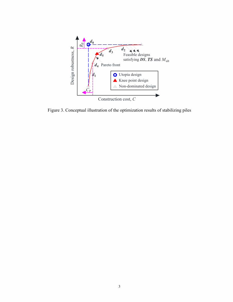
3

Figure 3. Conceptual illustration of the optimization results of stabilizing piles

d1

Construction cost, C

Utopia design

d5

d2

Des

ign

ro

bu

stnes

s, R d3

CP

Non-dominated design

Pareto front

RP

Feasible designs

satisfying DS, TS and Mult

d0

d4

Knee point design

4

Figure 4. Schematic diagram of the illustrative example

Pile geometric parameters

{D, S/D, L, X }

Rock surface

Initial slip surface

14 m

Pile position , X

Soil layer

A

Soil layer

B

O

Dep

th o

f

har

d r

ock

, H

C

20 m

5

(a) Design robustness R (b) Design safety E[FS2] (c) Design safety Pf

Figure 5. Effectiveness of the adopted SSM in deriving the design robustness and safety

6

(a) Design safety E[FS2]versus cost C (b) Design safety Pf versus cost C (c) Design robustness R versus cost C

Figure 6. Evaluation of the design safety, design robustness and construction cost for candidate designs in the design space DS

7

(a) Target stability TS of FST = 1.20 (b) Target stability TS of FST = 1.25

(c) Target stability TS of T = 2.6 (d) Target stability TS of T = 3.2

Figure 7. Influence of the target stability TS on the design results of the stabilizing piles

8

(a) Designs obtained with deterministic approach versus those with advanced framework

(target stability TS is set up as FST = 1.20)

(b) Designs obtained with probabilistic approach versus those with advanced framework

Figure 8. Designs obtained with conventional design approaches versus those with the

advanced design framework (Note: the vertical coordinate represents the ratio of the design

objective of the designs obtained with the conventional design approaches over that of the

designs obtained with advanced design framework)

9

(a) COV of cohesion (b) COV of friction angle (c) Vertical scale of fluctuation

Figure 9. Influence of the input statistical information of soil strength parameters on the variation of the stability of reinforced slope

(advanced framework versus deterministic approach: target stability FST = 1.20 and different percentiles of the inputs are taken)

10

(a) COV of cohesion (b) COV of friction angle (c) Vertical scale of fluctuation

Figure 10. Influence of the input statistical information of soil strength parameters on the variation of the stability of reinforced

slope (advanced framework versus probabilistic approach: different target reliability index T are studied)

1

Table 1. Statistical information of the uncertain input parameters (or noise factors) in the illustrative example

Uncertain input parameters Distribution Mean COV Scale of fluctuation

Horizontal, h Vertical, v

Soil strength

parameters a

Cohesion, c Lognormal 12.0 kPa 0.40 b 50.0 m 2.5 m

Friction angle, Lognormal 20.0 0.25 b 50.0 m 2.5 m

Structural

properties

Yielding strength of steel bar Normal 345103 kPa 0.05 c - -

Compression strength of concrete Normal 39103 kPa 0.12 c - -

Model error (true FS) – (calculated FS) Uniform The distribution range is [-0.02, 0.02]

Note: a the correlation coefficient between soil cohesion and soil friction angle is -0.5;

b data are from Cherubini (2000);

c data are from Wiśniewski et al. (2012).

2

Table 2. Deterministic parameters in the illustrative example

Category Parameter Value

Soil

Unit weight (kN/m3) 17.0

Bulk modulus (MPa) 330

Shear modulus (MPa) 150

Stabilizing piles

Unit weight (kN/m3) 25.0

Young’s modulus (GPa) 35.0

Steel reinforcement ratio (%) 1.0

Thickness of concrete protective cover (m) 0.05

Soil-pile interfaces

Normal stiffness (MPa/m) 550

Shear stiffness (MPa/m) 550

Cohesion (kPa) 12.0

Friction angle () 20.0

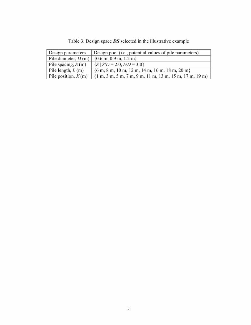
3

Table 3. Design space DS selected in the illustrative example

Design parameters Design pool (i.e., potential values of pile parameters)

Pile diameter, D (m) {0.6 m, 0.9 m, 1.2 m}

Pile spacing, S (m) {S | S/D = 2.0, S/D = 3.0}

Pile length, L (m) {6 m, 8 m, 10 m, 12 m, 14 m, 16 m, 18 m, 20 m}

Pile position, X (m) {1 m, 3 m, 5 m, 7 m, 9 m, 11 m, 13 m, 15 m, 17 m, 19 m}

4

Table 4. Optimal designs of the stabilizing piles obtained with the advanced design framework

Target stability TS

Number

of feasible

designs

Number

of non-

dominated

designs

Most preferred design

Pile design parameters d Cost, C

(C0 m3/m)

Design safety Design

robustness,

R D (m) S (m) L (m) X (m) E[FS2]

Factor

of safety

FST = 1.20 217 6 0.9 2.7 12.0 5.0 2.827 1.22 3.624 25.995

FST = 1.25 74 4 1.2 3.6 14.0 3.0 4.398 1.25 4.707 25.902

Reliability

index

T = 2.6 256 7 0.6 1.8 14.0 5.0 2.199 1.19 3.237 25.870

T = 3.2 111 5 0.6 1.8 14.0 5.0 2.199 1.19 3.237 25.870

5

Table 5. Optimal designs of the stabilizing piles obtained with the conventional geotechnical design approaches

Design approach

Pile design parameters d Cost, C

(C0 m3/m)

Design safety Design

robustness,

R D (m) S (m) L (m) X (m) E[FS2] Pf

Deterministic

approach

(FST = 1.2)

50th percentile 0.9 2.7 8.0 3.0 1.885 1.20 3.192 7.0610-4 24.834

40th percentile 1.2 2.4 12.0 5.0 5.655 1.30 3.969 3.6110-5 22.896

30th percentile The maximum FS2 of the candidate pile design is less than FST = 1.2, and no feasible

designs could be identified in the design space DS shown in Table 2.

Probabilistic

approach

T = 2.6 0.6 1.8 8.0 3.0 1.257 1.18 2.655 3.9710-3 23.953

T = 3.2 0.6 1.8 10.0 5.0 1.571 1.19 3.320 4.5110-4 25.201