Weierstraÿ-Institutfür Angewandte Analysis und Sto hastikim Fors hungsverbund Berlin e.V.Preprint ISSN 0946 8633Analyti al and numeri al aspe ts of time-dependentproblems with internal variablesPeter Gruber1, Dorothee Knees2, Sergiy Nesenenko3, Marita Thomas4submitted: November 17, 20091 Numeris he Mathematik, Johannes Kepler Universität Linz, Altenbergerstr. 69, 4040-Linz, Austria,email: peter.grubernuma.uni-linz.a .at2 Weierstrass Institute for Applied Analysis and Sto hasti s, Mohrenstr. 39, 10117 Berlin, Germanyemail: kneeswias-berlin.de3 Fa hberei h Mathematik, Te hnis he Universität Darmstadt, S hlossgartenstrasse 7,64289 Darmstadt, Germany, email: nesenenkomathematik.tu-darmstadt.de,Laboratoire Ja ques-Louis Lions, Universite Pierre et Marie Curie, Boite ourrier 187,75252 Paris Cedex 05, Fran e, email: nesenenkoann.jussieu.fr4 Humboldt-Universität zu Berlin, Mathemati al Institute, Unter den Linden 6, 10099 Berlin, Germany,email: thomasmathematik.hu-berlin.de No. 1460Berlin 2009

2000 Mathemati s Subje t Classi ation. 74C05, 74C10, 49N60, 65M60 .Key words and phrases. elasto-plasti ity, vis o-plasti ity, models of monotone type, existen e of solutions,monotone operator method, spatial regularity, Slant Newton Method, energeti formulation of rate-independentpro esses, temporal regularity.

Edited byWeierstraÿ-Institut für Angewandte Analysis und Sto hastik (WIAS)Mohrenstraÿe 3910117 BerlinGermanyFax: + 49 30 2044975E-Mail: preprintwias-berlin.deWorld Wide Web: http://www.wias-berlin.de/

Abstra tIn this paper some analyti al and numeri al aspe ts of time-dependent models with in-ternal variables are dis ussed. The fo us lies on elasto/vis o-plasti models of monotonetype arising in the theory of inelasti behavior of materials. This lass of problems in ludesthe lassi al models of elasto-plasti ity with hardening and vis ous models of the Norton-Ho type. We dis uss the existen e theory for dierent models of monotone type, give anoverview on spatial regularity results for solutions to su h models and illustrate a numeri- al solution algorithm at an example. Finally, the relation to the energeti formulation forrate-independent pro esses is explained and temporal regularity results based on dierent onvexity assumptions are presented.1 Introdu tionIn metalli materials various phenomena on the mi ros ale indu e ma ros opi ally inelasti be-havior: The hindering of the dislo ation motion by other dislo ations or grain boundaries ausehardening ee ts, whi h are observed on the ma ros opi s ale. The nu leation and growth ofgrain boundary avities initiate the development of mi ro ra ks whi h may ause the failure thewhole stru ture.From the phenomenologi al point of view the ma ros opi state of inelasti bodies is ompletelydetermined by the displa ement or deformation eld, the stress tensor and a nite number ofinternal variables representing internal pro esses on the mi ros ale. The orresponding ma ro-s opi models onsist of the balan e of for es, an evolution law for the internal variables and onstitutive equations whi h relate the stresses with the displa ement gradient and the internalvariables. A thermodynami ally onsistent framework for su h models is the lass of generalizedstandard materials dened by Halphen and Nguyen Son and the more general lass of models ofmonotone type introdu ed by Alber. From the mathemati al point of view these models lead to oupled systems of linear hyperboli /ellipti partial dierential equations and nonlinear ordinarydierential equations/in lusions. A typi al appli ation of su h models is elasto(vis o)-plasti itywith hardening at small strains. In the rate-independent ase an alternative energeti formula-tion for su h models was proposed by Mielke et al. in the last years. This formulation provides ageneral tool to rigorously analyze ee ts like damage, fra ture or hystereti behavior in magneti and ferroele tri bodies at both, small and nite strains. The aim of this paper is to review somere ent analyti al and numeri al aspe ts of models of this type.The starting point for the models dis ussed in this paper is the following: Given a time interval[0, T ] and a state spa e Q = U × Z let u : [0, T ] → U denote the generalized displa ementsand z : [0, T ] → Z the internal variables. It is assumed that U and Z are real, separable andreexive Bana h spa es. In the appli ations of plasti ity, typi al hoi es are Z = Lp(Ω) and U isidentied with a suitable subspa e of the Sobolev spa e W 1,p(Ω). The set Ω ⊂ R

d des ribes thephysi al body. In the rst hapters of this presentation the asso iated elasti energy Ψ : Q → Ris assumed to be quadrati and positive semidenite, i.e. we haveΨ(u, z) =

1

2〈A ( u

z ) , ( uz )〉1

where A =(

A11 A12A21 A22

): Q = U×Z → Q∗ is a linear, bounded symmetri and positive semideniteoperator. In addition to the elasti energy Ψ we also onsider the energy

E(t, u, z) = Ψ(u, z) − 〈b(t), u〉for given external loadings b ∈ C1([0, T ];U∗). The evolution law for the internal variable z is hara terized by a monotone, multivalued mapping G : Z → P(Z∗) with the property 0 ∈ G(0).Thereby U∗, Z∗ and Q∗ are the duals of the Bana h spa es U , Z and Q respe tively and P(Z∗)denotes the power set of Z∗. The assumptions on E and G are motivated by thermodynami al onsiderations whi h are arried out in Se tion 2.1. There also the link to elasto-plasti ity isexplained more detailed. The evolution model asso iated with E and G onsists of the for ebalan e equation (1.1) whi h is oupled with the evolution law (1.2) for the internal variable:Find absolutely ontinuous fun tions u ∈ AC([0, T ];U) and z ∈ AC([0, T ];Z) with z(0) = z0 ∈ Zsu h that for almost every t ∈ [0, T ] it holds0 = ∂uE(t, u(t), z(t)) = A11u(t) +A12z(t) − b(t), (1.1)

∂tz(t) ∈ G(−∂zE(t, u(t), z(t)) = G(−(A21u(t) +A22z(t))). (1.2)Systems of this stru ture onstitute the lass of models of monotone type introdu ed by Alber[1. The sub lass of generalized standard materials is obtained if in addition to the above it isassumed that G is the onvex subdierential of a onvex and proper fun tion. The parti ular hoi e G = ∂χK, where 0 ∈ K ⊂ Z is onvex and losed, and where χK denotes the hara teristi fun tion related to K, nally leads to the sub lass of rate-independent evolution models. Typi alexamples for these lasses of models are elasto-plasti ity in the small strain setting omprising forexample linear kinemati hardening. An example for a rate-dependent model is the vis o-plasti Norton-Ho model.The mathemati al analysis of rate-independent elasto-plasti models has its roots in the fun-damental ontributions by Moreau, Duvaut/Lions and Johnson, [32, 53, 78. More re ent in-vestigations, whi h also over rate-dependent models, are due to Alber/Chelminski [2, see also[47. If A and hen e Ψ are positive denite, i.e. if Ψ(u, z) ≥ α2 (‖u‖2

U + ‖z‖2Z) for all (u, z) ∈ Q,and if in addition G is maximal monotone, then lassi al results state the existen e of a uniquesolution (u, z) ∈ AC([0, T ];Q) for su iently regular given data b and z0, whi h satisfy a ertain ompatibility ondition.In ontrast to the positive denite ase it is quite hallenging to prove existen e results for(1.1)(1.2) if A is positive semidenite, only. Typi al examples for su h models are the elasti -perfe tly plasti Prandtl-Reuss model and models with linear isotropi hardening and we referto [53, 28, 47, 23 for the dis ussion of existen e questions. In Se tion 2.5 we present an existen eproof for a model with a positive semi-denite energy Ψ under the assumption that a ertain oupling ondition is satised between the operators A12 and A22. Here, we study the solvabilityfor u ∈ Lq(S;W 1,q(Ω)) and z ∈ AC(S;Lq(Ω)) for suitable q ∈ (1,∞).Apart from existen e results it is of great interest to gain more insight into the qualitativeproperties of solutions, su h as spatial or temporal regularity and stability. This knowledge isthe basis for the onstru tion of e ient and robust numeri al algorithms. Se tion 3 is devoted tothe dis ussion of spatial regularity results for solutions of models of monotone type. Dependingon the positivity properties of the free energy Ψ dierent regularity results may be a hieved.In the positive semi-denite ase one typi ally obtains the spatial regularity

σ ∈ L∞((0, T );H1lo (Ω))2

for the stress tensor σ. The basi observation enabling this result is the fa t that the omple-mentary energy, whi h is the onvex onjugate of the free energy, is positive denite with respe tto the generalized stresses, although the energy Ψ might not be positive denite. In addition tothe semidenite ase, for positive denite energies the following global spatial regularity resultsare available for domains with smooth boundary: For every δ > 0 it holdsu ∈ L∞((0, T );H

32−δ(Ω)) ∩ L∞((0, T );H2lo (Ω)), (1.3)

σ, z ∈ L∞((0, T );H12−δ(Ω)) ∩ L∞((0, T );H1lo (Ω)). (1.4)The proof of the global results relies on stability estimates for the solutions of (1.1)(1.2) and aree tion argument. A dis ussion on erning the optimality of (1.3)(1.4) as well as an overviewof the related literature is provided in Se tions 3.2 and 3.3. Moreover, we dis uss an examplewhi h shows that in spite of smooth data and a smooth geometry one should not expe t a omparable spatial regularity result for the time derivatives ∂tu and ∂tz.In Se tion 4 we dis uss and analyze a numeri al algorithm for solving rate-independent elasto-plasti models. After a time dis retization with an impli it Euler s heme the time in rementalproblem an be reformulated as a quasilinear ellipti system of partial dierential equations todetermine the displa ements at time step tk from the displa ements and internal variables ofthe previous time step. The internal variable of the urrent time step then an be al ulatedvia a straightforward update formula. Sin e the nonlinear ellipti operator is not Gâteaux-dierentiable, lassi al Newton methods are not appli able for solving the PDE. Instead wedis uss an approa h where we use a so- alled slanting fun tion instead of the derivative resultingin a Slant Newton Method. The behavior of this algorithm is illustrated at some examples.In the last se tion, Se tion 5, we fo us on rate-independent models of the type (1.1)-(1.2) with

G = ∂χK. As already mentioned, in this ase the model (1.1)(1.2) an be reformulated in theglobal energeti framework for rate-independent evolution pro esses introdu ed by Mielke andTheil [70. Indeed we will show in Se tion 5 that the model is equivalent to the following problem:Find a pair (u, z) : [0, T ] → Q with (u(0), z(0)) = (u0, z0) whi h for every t ∈ [0, T ] satisesstability relation (S) and the energy balan e (E)(S) for every (v, ζ) ∈ Q we have E(t, u(t), z(t)) ≤ E(t, v, ζ) + R(ζ − z(t)),(E) E(t, u(t), z(t)) +

∫ t

0R(∂tz(τ))dτ = E(0, u(0), z(0)) +

∫ t

0∂tE(τ, u(τ), z(τ))dτ,where R : Z → [0,∞] is the onvex onjugate of the hara teristi fun tion χK and hen e is onvex and positively homogeneous of degree one.The energeti framework allows for more general energies E , whi h not ne essarily have aquadrati stru ture or stri t onvexity properties, or whi h might not be Gâteaux dierentiablewith respe t to u or z. The energeti formulation of rate-independent pro esses provides a gen-eral tool, whi h also applies to further physi al phenomena like damage, fra ture, shape memoryee ts or ferroele tri behavior. Sin e the energy E is not ne essarily stri tly onvex, solutionsmay o ur whi h are dis ontinuous in time. A general existen e theorem is ited. Subsequentit is investigated to what extend dierent onvexity assumptions on the energy yield solutionswhi h are ontinuous, Hölder- ontinuous or even Lips hitz- ontinuous in time. These onvexityassumptions are dis ussed for dierent examples modeling elasto-plasti ity, shape memory ee tsand damage. 3

2 Elasto(vis o)-plasti models of monotone type2.1 Thermodynami frameworkIn this subse tion we show that the problem (1.1) - (1.2) is thermodynami ally admissible. Westart with a ma ros opi model des ribing inelasti response of solids at small strains in the mostgeneral form, and then we extra t a sub lass of models, for whi h the Clausius-Duhem inequalityis naturally satised. This sub lass of models onsists of problems of the type (1.1) - (1.2).Setting of the problemFor the subsequent analysis we restri t ourselves only to the 3-dimensional ase, although allof our results hold in any spa e-dimension. Let Ω ⊂ R3 be a bounded domain with Lips hitzboundary ∂Ω and let S3 be the linear spa e of symmetri 3×3-matri es. Let Te denote a positivenumber (time of existen e). For 0 ≤ t ≤ Te we introdu e the spa e-time ylinder Ωt = Ω× (0, t).The initial boundary value problem for the unknown displa ement u(x, t) ∈ R

3, the Cau hystress tensor T (x, t) ∈ S3 and the ve tor of internal variables z(x, t) ∈ RN in a quasi-stati setting is formed by the equations

− divx T (x, t) = b(x, t), (2.1)T (x, t) = A(ε(∇xu(x, t)) −Bz(x, t)), (2.2)

∂

∂tz(x, t) ∈ f(ε(∇xu(x, t)), z(x, t)), (2.3)whi h must hold for all x ∈ Ω and all t ∈ [0,∞). The initial value for z(x, t) and the Diri hletboundary ondition for u(x, t) are given by

z(x, 0) = z(0)(x), for x ∈ Ω, (2.4)u(x, t) = γ(x, t), for (x, t) ∈ ∂Ω × [0,∞). (2.5)Here ∇xu(x, t) denotes the 3× 3-matrix of rst order derivatives of u, the deformation gradient,

(∇xu(x, t))T denotes the transposed matrix, and

ε(∇xu(x, t)) =1

2(∇xu(x, t) + (∇xu(x, t))

T ) ∈ S3,is the strain tensor. The linear mapping B : RN 7→ S3 is a proje tor with εp(x, t) = Bz(x, t),where εp ∈ S3 is a plasti strain tensor. We denote by A : S3 → S3 a linear, symmetri , positivedenite mapping, the elasti ity tensor. The given data of the problem are the volume for e

b : Ω × [0,∞) 7→ R3, the boundary displa ement γ : ∂Ω × [0,∞) 7→ R

3, and the initial data forthe ve tor of the internal variables z(0) : Ω 7→ RN . The given fun tion f : D(f) ⊆ S3×R

N 7→ 2RNis a onstitutive fun tion with the domain D(f).The dierential in lusion (2.3) with a pres ribed fun tion f together with the equation (2.2)dene the material behavior. They are the onstitutive relations whi h model the elasto(vis o)-plasti behavior of solid materials at small strains, whereas (2.1) is the for e balan e arising fromthe onservation law of linear momentum.The initial boundary value problem (2.1) - (2.5) is written here in the most general form and,to the best of our knowledge, in ludes all elasto(vis o)-plasti models at small strains used in4

the engineering. To guarantee that by equations (2.1) - (2.5) a thermodynami ally admissiblepro ess is des ribed, we laim the existen e of a free energy density ψ : D(f) → [0,∞) su h thatthe Clausius-Duhem inequalityρ∂

∂tψ(ε(∇xu), z) − divx(Tut) − b · ut ≤ 0 (2.6)holds in Ω × (0,∞) for all solutions (u, T, z) of (2.1) - (2.5). The fun tion ρ denotes the massdensity and it is assumed to be onstant. The requirement (2.6) restri ts the possible hoi es of

f . Indeed, let (u, z) be a su iently smooth solution of (2.1) - (2.6). Firstly, we note that thesymmetry of the stress tensor impliesT · ε(∇xut) = T · ∇xut = divx(T Tut) − (divx T ) · ut.Then, as a dire t onsequen e of the Clausius-Duhem inequality (2.6), one gets with the help ofthe previous relation and the symmetry of T the following inequality

ρ∇εψ · ε(∇xut) + ρ∇zψ · zt − divx(Tut) − b · ut

= ρ∇εψ · ε(∇xut) + ρ∇zψ · zt − T · ε(∇xut) = (ρ∇εψ − T ) · ε(∇xut) + ρ∇zψ · zt≤ 0.Due to the arbitrariness of the strain rate ε = ε(∇xut), we on lude that

ρ∇εψ(ε, z) = T, (2.7)ρ∇zψ(ε, z) · ζ ≤ 0 (2.8)for every ζ ∈ f(ε, z) and for all (ε, z) ∈ D(f). Inequality (2.8) is alled the dissipation inequality.Therefore, we all the onstitutive equations (2.2) and (2.3) thermodynami ally admissible if afree energy density ψ exists su h that (2.7) and (2.8) are satised.Now it is easy to extra t a sub lass of onstitutive fun tions f , for whi h the dissipation inequality(2.8) is naturally fullled. This sub lass onsists of those fun tions f , whi h an be written inthe form

f(ε, z) = g(−ρ∇zψ(ε, z)), (2.9)with a suitable free energy density ψ : D(f) → [0,∞) satisfying (2.7), and with a suitablemonotone fun tion g : D(g) ⊆ RN → 2RN with the property 0 ∈ g(0).Relations (2.2) and (2.7) allow us to nd the pre ise form of the free energy density: Integrating(2.7) with respe t to ε we an easily obtain that

ρψ(ε, z) =1

2A(ε−Bz) · (ε−Bz) + ψ1(z)with a suitable fun tion ψ1 : D(ψ1) ⊆ R

N → [0,∞) as a onstant of integration. For mathemat-i al reasons we assume in this hapter that the free energy density ψ has a spe ial form, namelyit is a positive semi-denite quadrati form given byρψ(ε, z) =

1

2A(ε−Bz) · (ε−Bz) +

1

2(Lz) · z (2.10)with a symmetri , non-negative N ×N -matrix L. Dierentiating (2.10) with respe t to z yields

−ρ∇zψ(ε, z) = BTA(ε−Bz) − Lz = BTT − Lz.5

In view of these onsiderations the initial boundary value problem (2.1) - (2.5) an be written as− divx T (x, t) = b(x, t), (2.11)

T (x, t) = A(ε(∇xu(x, t)) −Bz(x, t)), (2.12)∂

∂tz(x, t) ∈ g(BTT (x, t) − Lz(x, t)) (2.13)z(x, 0) = z(0)(x), (2.14)for all x ∈ Ω and all t ∈ [0,∞), together with the Diri hlet boundary ondition

u(x, t) = γ(x, t) for x ∈ ∂Ω, t ∈ [0,∞). (2.15)The initial boundary value problem (2.11) - (2.15) is alled the problem/model of monotonetype. As we have already mentioned in the introdu tion, this lass of models was introdu ed byAlber in [1 and it naturally generalizes the lass of problems of generalized standard materialsproposed by Halphen and Nguyen Quo Son. We re all that the models of generalized standardmaterials are formed by equations (2.11) - (2.15) with the monotone fun tion g given expli itlyby the subdierential of a proper onvex fun tion. Typi al examples for models of monotonetype are elasto-plasti models with linear or nonlinear hardening (for more details, onsult thebook [1, Chapter 3.3).First existen e results for the lassi al model of perfe t plasti ity (Prandtl-Reuss-model) werederived in [76, 32, 53. Sin e the elasti energy in this ase is positive semidenite, only, thedispla ements in general belong to the spa e of bounded deformations, only, [102, 104, 105. Theexisten e theory for elasto-plasti models with a positive denite energy (like elasto-plasti itywith linear kinemati hardening) was initiated by Johnson [54, we refer to the monographs[47, 39 for a histori al survey on the subje t. In the late 90ies these results were extended tomodels of monotone type with general maximal monotone fun tions g, still assuming that theenergy is positive-denite, [1, 2. In [3, 23, 22, 24, 82, 84, 85 an approa h for the derivationof the existen e of solutions to the problem (2.11) - (2.15) initiated in [1 was ontinued andextended to parti ular models of monotone type with a positive semi-denite energy. In thepresent paper, we briey dis uss the existen e result in [2 for models with a positive deniteenergy in order to point out the main dieren es and di ulties whi h arise in the treatment ofmonotone problems with a positive semi-denite energy. An existen e proof for a spe ial lasswith a positive semi-denite energy is dis ussed afterwards.2.2 Fun tion spa es and notationFor m ∈ N, q ∈ [1,∞], we denote by Wm,q(Ω,Rk) the Bana h spa e of Lebesgue integrablefun tions having q-integrable weak derivatives up to order m. This spa e is equipped with thenorm ‖ · ‖m,q,Ω. If m = 0 we also write ‖ · ‖q,Ω. If m is not integer, then the orrespondingSobolev-Slobode kij spa e is denoted by Wm,q(Ω,Rk). We set Hm(Ω) = Wm,2(Ω), f. [42.We hoose the numbers p, q satisfying 1 < p, q < ∞ and 1/p + 1/q = 1. For su h p and q one an dene the bilinear form on the produ t spa e Lp(Ω,Rk) × Lq(Ω,Rk) by(ξ, ζ)Ω =

∫

Ωξ(x) · ζ(x)dx.6

If (X,H,X∗) is an evolution triple (known also as a Gelfand triple or spa es in normal posi-tion), thenWp,q(0, Te;X) =

u ∈ Lp(0, Te;X) | u ∈ Lq(0, Te;X

∗)is a separable reexive Bana h spa e furnished with the norm

‖u‖2Wp,q

= ‖u‖2Lp(0,Te;X) + ‖u‖2

Lq(0,Te;X∗),where the time derivative u of u is understood in the sense of ve tor-valued distributions. We re- all that the embedding Wp,q(0, Te;X) ⊂ C([0, Te],H) is ontinuous ([50, p. 4, for instan e). Fi-nally we frequently use the spa esW k,p(0, Te;X), whi h onsist of Bo hner measurable fun tionswith a p-integrable weak derivatives up to order k. Observe thatW2,2(0, Te;X) = W 1,2(0, Te;X).2.3 Basi properties of the operator of linear elasti ityHere, we state the assumptions on the oe ient matri es in (2.11) - (2.13):A ∈ L∞(Ω,Lin(S3,S3)) is symmetri and uniformly positive denite,i.e. there exists α > 0 su h that A(x)ε · ε ≥ α ‖ε‖2 for all ε ∈ S3 and a.e. x ∈ Ω,L ∈ L∞(Ω; Lin(RN ,RN )) is symmetri and positive semi-denite. (2.16)Sin e the linear mapping A(x) : S3 → S3 is uniformly positive denite, a new bilinear form on

Lp(Ω,S3) × Lq(Ω,S3) an be dened by[ξ, ζ]Ω = (Aξ, ζ)Ω.From [108, Theorem 4.2 we re all an existen e theorem for the following boundary value problemdes ribing linear elasti ity:

−divxT (x) = b(x), for x ∈ Ω, (2.17)T (x) = A(x)(ε(∇xu(x)) − εp(x)), for x ∈ Ω, (2.18)

u(x) =γ(x), for x ∈ ∂Ω. (2.19)To given b ∈ W−1,q(Ω,R3), εp ∈ Lp(Ω,S3) and γ ∈ W 1,p(Ω,R3) the problem (2.17) - (2.19) hasa unique weak solution (u, T ) ∈ W 1,p(Ω,R3) × Lp(Ω,S3) with 1 < p < ∞ and 1/p + 1/q = 1provided A ∈ C(Ω,Lin(S3,S3)) and Ω is of lass C1. For p = 2 this result for the problem (2.17)- (2.19) holds provided that A satises ondition (2.16) and that Ω is a Lips hitz domain. Forb=γ=0 there is a onstant C > 0 su h that the solution of (2.17) - (2.19) satises the inequality

‖ε(∇xu)‖p,Ω ≤ C‖εp‖p,Ω.Denition 2.1. For every εp ∈ Lp(Ω,S3) we dene a linear operator Pp : Lp(Ω,S3) → Lp(Ω,S3)by Ppεp = ε(∇xu), where u ∈ W 1,p0 (Ω,R3) is the unique weak solution of (2.17) - (2.19) for thegiven fun tion εp and b = γ = 0.Let the subset Gp ⊂ Lp(Ω,S3) be dened by

Gp = ε(∇xu) | u ∈W 1,p0 (Ω,R3).The following lemma states the main properties of Pp.7

Lemma 2.2. For every 1 < p <∞ the operator Pp is a bounded proje tor onto the subset Gp ofLp(Ω,S3). The proje tor (Pp)

∗, whi h is the adjoint with respe t to the bilinear form [ξ, ζ]Ω onLp(Ω,S3) × Lq(Ω,S3), satises

(Pp)∗ = Pq, where 1

p + 1q = 1.This implies ker(Pp) = Hp

sol with Hpsol = ξ ∈ Lp(Ω,S3) | [ξ, ζ]Ω = 0 for all ζ ∈ Gq.The proje tion operator

Qp = (I − Pp) : Lp(Ω,S3) → Lp(Ω,S3)with Qp(Lp(Ω,S3)) = Hp

sol is a generalization of the lassi al Helmholtz proje tion.Corollary 2.3. Let (BTAQpB + L)T be the adjoint operator ofBTAQpB + L : Lp(Ω,RN ) → L

p(Ω,RN )with respe t to the bilinear form (ξ, ζ)Ω on the produ t spa e Lp(Ω,RN )×Lq(Ω,RN ). Then(BTAQpB + L)T = BTAQqB + L : Lq(Ω,RN ) → L

q(Ω,RN ).Moreover, the operator BTAQ2B + L is non-negative and self-adjoint.The last result in this orollary is proved in [2.Remark 2.4. If the matrix L is uniformly positive denite, then the operator BTAQ2B + L ispositive denite.Remark 2.5. Hpsol is a reexive Bana h spa e with dual spa e Hq

sol.Finally we ite an existen e result for the following Cau hy problem in a Hilbert spa e H witha maximal monotone operator A : D(A) ⊂ H → 2H :d

dtu(t) +A(u(t)) ∋ f(t), (2.20)

u(0) = u0. (2.21)Theorem 2.6. [11, 97 Assume that u0 ∈ D(A). If f ∈ W 1,1(0, Te;H), then the Cau hyproblem (2.20) - (2.21) has a unique solution u ∈ W 1,∞(0, Te;H). If A = ∂φ, where ∂φ is thesubdierential of a proper onvex lower-semi- ontinuous fun tion, then for every f ∈ L2(0, Te;H)the problem (2.20) - (2.21) has a unique solution u ∈W 1,2(0, Te;H).2.4 Existen e of solutions in the ase of positive denite energyIt is already known (see [2, Theorem 1.3) that the initial boundary value problem (2.11) - (2.15)has a unique solution provided the mapping z 7→ g(z) is maximal monotone and the matrix L isuniformly positive denite. We now state the existen e result due to Alber and Chelminski [2.Theorem 2.7. Assume that the oe ient matri es satisfy (2.16), that in addition L in (2.13)is uniformly positive denite and that the mapping g : RN → 2RN is maximal monotone with8

0 ∈ g(0). Suppose that b ∈ W 2,1(0, Te;L2(Ω,R3)) and γ ∈ W 2,1(0, Te;H

1(Ω,R3)). Finally,assume that z(0) ∈ L2(Ω,RN ) and that there exists ζ ∈ L2(Ω,RN ) su h thatζ(x) ∈ g(BTT (0)(x) − L(x)z(0)(x)), a.e. in Ω, (2.22)where (u(0), T (0)) is a weak solution of the elasti ity problem (2.17)-(2.19) to the data b = b(0),

εp = Bz(0), γ = γ(0).Then for every Te > 0 there is a unique solution of the initial boundary value problem (2.11) -(2.15)(u, T, z) ∈W 1,2(0, Te;H

1(Ω,R3) × L2(Ω,S3) × L2(Ω,RN )).If g = ∂χK , where ∂χK is the subdierential of the hara teristi fun tion asso iated with the onvex, losed set 0 ∈ K ⊂ RN , then it is su ient to require b ∈ W 1,2(0, Te;L

2(Ω,R3)) andγ ∈W 1,2(0, Te;H

1(Ω,R3)).Remark 2.8. We note that L is uniformly positive denite if and only if the free energy density ψis a positive denite quadrati form on S3 ×RN . The onstitutive equations for linear kinemati hardening satisfy this requirement, while models for linear isotropi hardening are not overed.The main idea of the proof of Theorem 2.7 onsists in the redu tion of the equations (2.11) -(2.15) to an autonomous evolution in lusion in a Hilbert spa e governed by a maximal monotoneoperator. To this evolution in lusion Theorem 2.6 is applied, whi h allows to on lude that theinitial boundary value problem (2.11) - (2.15) has a (unique!) solution. For the redu tion itis ru ial that the oe ient fun tion L is uniformly positive denite. To indi ate the maindieren es between the ase of a positive denite free energy density ompared to a positivesemi-denite density we briey sket h the proof of Theorem 2.7. Details an be found in [2.Proof. We note that equations (2.11) - (2.12), (2.15) form a boundary value problem for the omponents (u(t), T (t)) of the solution. Obviously one has an additive de omposition

(u(t), T (t)) = (u(t), T (t)) + (v(t), σ(t)),with the solution (v(t), σ(t)) of the Diri hlet boundary value problem (2.17) - (2.19) to the datab = b(t), γ = γ(t), εp = 0, and with the solution (u(t), T (t)) of the problem (2.17) - (2.19) to thedata b = γ = 0, εp = Bz(t). We thus obtain

ε(∇xu) −Bz = (P2 − I)Bz + ε(∇xv).Inserting this into (2.12) we re eive that (2.13) an be rewritten in the formzt(t) ∈ G

(− (BTAQ2B + L)z(t) +BTσ(t)

), (2.23)where G : D(G) ⊂ L2(Ω,RN ) → 2L2(Ω,RN ) dened by G(ξ) = ξ ∈ L2(Ω,RN ) | ξ(x) ∈

g(ξ(x)) a.e.. The fun tion σ, as a solution of the problem (2.17) - (2.19) to the given datab, γ, is onsidered as known.A ording to Remark 2.4 the operator BTAQ2B + L is positive denite, therefore the equation(2.23) an be redu ed to an autonomous evolution equation in L2(Ω,RN ) using the transforma-tion h(t) = −(BTAQ2B + L)z(t) +BTσ(t). It then reads as

ht(t) + C(h(t)) ∋ BTσt(t) with C(ξ) = (BTAQ2B + L)G(ξ) for ξ ∈ L2(Ω,RN ). (2.24)9

The ru ial step in the proof is that the operator C is maximal monotone with respe t to thenew s alar produ t [[ξ, ξ]] := ((BTAQ2B+L)−1ξ, ξ) (see [2). This s alar produ t is well dened,sin e the operator BTAQ2B+L is positive denite due to the uniform positivity of L. Therefore,Theorem 2.6 an be applied to (2.24) in L2(Ω,RN ) equipped with the s alar produ t [[ξ, ξ]] toderive the existen e and uniqueness of solutions. The assumption (2.22) guarantees that theinitial value h(0) belongs to the domain of the operator C. Substituting the solution of (2.23),whi h exists due to the equivalen e of (2.23) and (2.24), into the boundary value problem formedby equations (2.11) - (2.12) and (2.15) yields the existen e of (u, T ) by the existen e theory forlinear ellipti problems.2.5 Existen e of solutions in the ase of a positive semi-denite energyAs we saw in the proof of Theorem 2.7 the positivity of L plays the essential role: It allowed todene a new s alar produ t in L2(Ω,RN ), with respe t to whi h the operator C from (2.24) ismaximal monotone so that Theorem 2.6 is appli able. Obviously, this strategy annot be appliedif L is only positive semi-denite and one has to over ome this di ulty. In the following werestri t ourselves to a sub lass of problems of monotone type with a positive semi-denite freeenergy density, for whi h the existen e of solutions an be veried. Existen e theorems for theentire lass of models of monotone type are still an open problem. For simpli ity, we assumethat the oe ient matri es in (2.11) - (2.13) are independent of x.Under the assumption that g is single-valued and that KerB + KerL = RN , the authors of[3 showed that the initial boundary value problem (2.11) - (2.15) is equivalent to the followingproblem: for all t ∈ [0,∞) and x ∈ Ω

− divx T (x, t) = b(x, t), (2.25)T (x, t) = A

(ε(∇xu(x, t)) − εp(x, t)

), (2.26)

∂tεp(x, t) = g1

(T (x, t),−z(x, t)

), (2.27)

∂tz(x, t) = g2

(T (x, t),−z(x, t)

), (2.28)

u(x, t) = γ(x, t), (x, t) ∈ ∂Ω × [0,∞), (2.29)εp(x, 0) = ε(0)p (x), z(x, 0) = z(0)(x). (2.30)Here the ve tor of internal variables z(x, t) is split into two parts, i.e. z(x, t) = (εp(x, t), z(x, t)) ∈

S3 × RN−6. We assume for simpli ity that ε(0)p (x) = 0. The fun tions g1 : S3 × R

N−6 → S3and g2 : S3 × RN−6 → R

N−6 are given su h that (T, y) → (g1(T, y), g2(T, y)) : RN → R

N is amonotone mapping.Following [3 we rewrite the problem (2.25) - (2.29) in terms of an operator H : F (ΩTe ,S3) →F (ΩTe ,S3), where F (ΩTe ,S3) denotes the set of all fun tions mapping ΩTe to S3. The operatorH is dened by the following rule: For given T and z(0) let (h, z) be a solution of the problem

h(x, t) = g1(T (x, t),−z(x, t)

) for (x, t) ∈ ΩTe , (2.31)∂tz(x, t) = g2

(T (x, t),−z(x, t)

) for (x, t) ∈ ΩTe , (2.32)z(x, 0) = z(0)(x) for x ∈ Ω, (2.33)Then the operator H on F (ΩTe ,S3) is given by H(T ) = h. In terms of the operator H the10

problem (2.25) - (2.29) reads as follows: for all (x, t) ∈ ΩTe

−divxT (x, t) = b(x, t), (2.34)T (x, t) = A

(ε(∇xu(x, t)) − εp(x, t)

), (2.35)

∂tεp(x, t) = H(T ), (2.36)εp(x, 0) = 0, (2.37)u(x, t) = γ(x, t), (x, t) ∈ ∂Ω × [0,∞). (2.38)Now we an state the existen e result of [82 for the problem (2.34) - (2.38).Theorem 2.9. Let 2 ≤ p < ∞ and 1 < q ≤ 2 be numbers with 1/p + 1/q = 1. Assume that

H : Lp(ΩTe ,S3) → Lq(ΩTe ,S3) is maximal monotone and that the inverse H−1 is lo ally boundedat 0 1 and strongly oer ive, i.e. either D(H−1) is bounded or D(H−1) is unbounded and〈v∗, v〉‖v‖q,ΩTe

→ +∞ as ‖v‖q,ΩTe→ ∞, v∗ ∈ H−1(v).Suppose that b ∈ Lp(ΩTe ,R

3) and γ ∈ Lp(0, Te,W1,p(Ω,R3)). Then there exists a solution of theproblem (2.34) - (2.38)

u ∈ Lq(0, Te;W1,q(Ω,R3)), T ∈ Lp(ΩTeS3), εp ∈W 1,q(0, Te, L

q(Ω,S3)).Remark 2.10. The monotoni ity of H is implied by the monotoni ity of the mapping (T, y) →(g1(T, y), g2(T, y)) (see [3, Lemma 4.1).Remark 2.11. To gain the existen e of solutions to (2.25) - (2.29) one has to he k rst whetherthe operator H : Lp(ΩTe ,S3) → Lq(ΩTe ,S3) is well dened, i.e. whether the problem (2.31)-(2.33) has a solution (not ne essary unique). Then apply Theorem 2.9.Remark 2.12. The proof of Theorem 2.9 in [82 ontains a gap, although the result remains true.The operator dened in Lemma 4.1 of [82 is not maximal monotone as it is stated there. Theproof of this is given in the end of this se tion.In [3 Theorem 2.9 is proved for H with polynomial growth and under the additional assumptionthat H is oer ive. The last assumption auses there di ulties in the derivation of the existen eof the solutions to the model of nonlinear kinemati hardening (see the next se tion for moredetails). In order to show the oer ivity of the operator H dened by the onstitutive relations(spe i hoi e of the fun tions g1 and g2) of nonlinear kinemati hardening, the authors of [3had to impose a restri tion on the exponents in the onstitutive relations for the dierent internalvariables. The approa h initiated in [82 is a tually based on the onstru tions in [3 and repeatsthe main steps of that work with the major dieren e that the general duality prin iple for thesum of two operators from [9 is used to obtain the existen e of the solutions to the problem(2.34) - (2.38). The appli ation of this duality prin iple allows to avoid the oer ivity assumptionon H. Here we present the improved version of the proof of Theorem 2.9 presented in [82.Proof. Let us denote

W = Lp(Ω,S3), W = Lp(0, Te;W ), X = Hpsol(Ω,S3), X = Lp(0, Te;X).1An operator A : V → 2V ∗ is alled lo ally bounded at a point v0 ∈ V if there exists a neighborhood U of v0su h that the set

A(U) = Av | v ∈ D(A) ∩ U is bounded in V ∗. 11

Repeating word by word the proof of Theorem 2.7 one an redu e the initial-boundary valueproblem (2.34) - (2.38) to the following abstra t equationLεp = H

(−AQpεp + σ

), (2.39)where the linear operator L : W → W∗ is dened by

Lη = ∂tη with D(L) = η ∈Wp,q(0, Te;W ) | η(0) = 0.The fun tion σ in (2.39) is given as in the proof of Theorem 2.7. Applying the operator Qq to(2.39) from the left formally and denoting τ = Qqεp we arrive at the equationLτ = QqH

(−Aτ + σ

), (2.40)where now L : X → X ∗ denotes the operator

Lη = ∂tη with D(L) = η ∈Wp,q(0, Te;X) | η(0) = 0.The strategy of Theorem 2.7 is not appli able here, sin e the omposition of two operators,one of them being monotone, ξ → QqH(− Aξ + σ

) is not monotone in general. It turns outthat applying the general duality prin iple (see [9) it is possible to release the monotoneoperator from another operator preserving its monotoni ity property and use the lassi al theoryof monotone operators. This is the main idea of the proof of Theorem 2.9.By the general duality prin iple [9, the in lusion (2.40) in X is equivalent to the followingin lusion in X ∗

L−1AQqw + H−1w ∋ σ, w ∈ X ∗. (2.41)Indeed, (2.40) holds i there exists v ∈ Lτ ∩Qqw with w = H(−Aτ + σ). Taking the inverse ofthe operators L and H gives (2.41). Thus, if we an solve (2.41), by the equivalen e we obtainthat the problem (2.40) has a solution as well.Due to Lemma 2.13 here below the operator L−1AQq : D(L−1AQq) ⊂ X ∗ → X is linear andmaximal monotone.Now we an show that (2.41) has a solution. Note rst that the operator H−1 is maximalmonotone as the inverse of a maximal monotone operator. Sin e H−1 is lo ally bounded at 0,by Lemma III.24 2 in [48 the point 0 belongs to the interior of D(H−1) = R(H). Therefore, theoperators L−1AQq and H−1 satisfy the onditionD(L−1AQq) ∩ intD(H−1) 6= ∅,yielding that the sum L−1AQq + H−1 is maximal monotone (by Theorem II.1.7 in [11). The oer ivity of H−1 implies the oer ivity of the sum, i.e.

⟨L−1AQqv + v∗, v

⟩

‖v‖ ≥ 〈v∗, v〉‖v‖ → +∞ as ‖v‖ → ∞, v∗ ∈ H−1(v).Theorem III.2.10 in [83 guarantees that the maximal monotone and oer ive operator L−1AQq+

H−1 is surje tive. Thus, equation (2.41) is solvable and, as onsequen e, problem (2.40) has asolution.2This result is proved in a Hilbert spa e, but it an be easily generalized to reexive Bana h spa es.12

The onstru tion of the solution of the problem (2.34) - (2.38) an be now performed as in [3:Let (v(t), σ(t)) be the solution of the Diri hlet boundary value problem (2.17) - (2.19) to thedata b = b(t), γ = γ(t), εp = 0 and let τ ∈ X be the unique solution of (2.40). With the fun tionτ let εp ∈W 1,q(0, Te, L

q(Ω,S3)) be the solution of∂tεp(t) = H

(−Aτ(t) + σ(t)

), for a.e. t ∈ (0, Te) (2.42)

εp(0) = 0. (2.43)Moreover, by the linear ellipti theory, there is a unique solution (u(t), T (t)) of problem (2.17) -(2.19) to the data b = γ = 0, εp = εp(t). The solution of (2.34) - (2.38) is now given as follows(u, T, εp) = (u+ v, T + σ, εp) ∈ Lq(0, Te;W

1,q(Ω,R3)) × Lp(ΩTeS3) ×W 1,q(0, Te, Lq(Ω,S3)).To see that (u, T, εp) satises (2.36), we apply the operator Qq to (2.42) - (2.43) from the leftand obtain

∂t(Qqεp) = QqH(−Aτ(t) + σ(t)

)= ∂tτ, Qqεp(0) = τ(0) = 0.The last line implies that Qqεp = τ . Thus

T = T + σ = −AQqεp + σ = −Aτ + σ ∈ Lp(ΩTeS3).The last observation ompletes the proof.Lemma 2.13. The operator L−1AQq : D(L−1AQq)⊂X ∗ → X is linear and maximal monotone.Proof. A ording to Theorem 2.7 in [83, the operator L−1AQq is maximal monotone, if it is adensely dened losed monotone operator su h that its adjoint (L−1AQq)∗ is monotone. Sin eall these properties of L−1AQq an be easily established, we leave their veri ation to the reader.More details an be also found in [81.Now we prove the result announ ed in Remark 2.12.Lemma 2.14. The operator QpL−1 : W∗ → W is not maximal monotone (we use the notationsintrodu ed above).Proof. Note rst of all that the following identity

QpL−1v = L−1Qqv (2.44)holds for all v ∈ D(QpL−1) = D(L−1) 3. The previous identity (2.44) follows easily fromPpL−1v = L−1Pqv, (2.45)whi h holds for v ∈ D(L−1). Relation (2.45) an be proved as follows: Choose v ∈ D(L−1).Then, a ording to the denition of Pp, the boundary value problem

− divAε(∇u(x, t)) = − divAv(x, t) for x ∈ Ω, (2.46)u(x, t) = 0 for x ∈ ∂Ω, (2.47)3Re all that D(L−1) = z ∈ W∗ |

R t

0z(s)ds ∈ W 13

has a unique solution u(t) ∈W 1,q0 (Ω,R3), i.e. the fun tion u satises the equation

(Aε(∇u(t)), ε(∇φ))Ω = (Av(t), ε(∇φ))Ω, for all φ ∈W 1,p0 (Ω,R3).Similarly, we obtain that the problem

− divAε(∇w(x, t)) = − divA(∫ t

0v(x, s)ds

) for x ∈ Ω,

w(x, t) = 0 for x ∈ ∂Ωhas a unique solution w(t) ∈W 1,p0 (Ω,R3). Integrating (2.46) we get that the identity

(Aε

(∇

∫ t

0u(s)ds

), ε(∇φ)

)Ω

=(A

(∫ t

0v(s)ds

), ε(∇φ)

)Ωholds for all φ ∈W 1,p

0 (Ω,R3). Thus, by the denition of Pp, we have that w(t) =∫ t0 u(s)ds. Thisproves (2.45).Next we show that the operator QpL−1 is not maximal monotone. To this end, onsider afun tion ψ ∈ W ∗ su h that ψ = ε(∇u) with u ∈ W 1,q

0 (Ω,R3) and ε(∇u) 6∈ W for any p > q(sin e ε(∇u) 6∈ D(L−1) ). Obviously, su h a fun tion u is the solution of the problem− divAε(∇u) = − divAψ, u ∈W 1,q

0 (Ω,R3).The last relation implies that ψ ∈ R(Pq) and onsequently that ψ ∈ kerQq.To show that QpL−1 is not maximal monotone, we need to nd a pair (y∗, y) ∈ W ×W∗ su hthat the inequality(QpL−1v − y∗, v − y)Ω ≥ 0 (2.48)holds for all v ∈ D(L−1), but (y∗, y) 6∈ Graph (QpL−1). Take any v ∈ D(L−1). Set y = v+ψ with

ψ from above and y∗ = L−1Qqy, i.e. y∗ = L−1Qqv = QpL−1v. Then (QpL−1v− y∗, v− y)Ω = 0.Therefore (2.48) is fullled for all v ∈ D(L−1), but v + ψ 6∈ D(QpL−1). Thus, the proof is omplete.2.6 Model of nonlinear kinemati hardeningWe apply Theorem 2.9 to the model of nonlinear kinemati hardening. It onsists of the equations( f. [1, 3)−divxT = b, (2.49)

T = A(ε(∇xu) − εp

), (2.50)

∂tεp = c1|T − k(εp − εn)|r T − k(εp − εn)

|T − k(εp − εn)| , (2.51)∂tεn = c2|k(εp − εn)|m k(εp − εn)

|k(εp − εn)| , (2.52)εn(0) = ε0n, εp(0) = 0, (2.53)

u = γ, x ∈ ∂Ω, (2.54)14

where c1, c2, κ > 0 are given onstants and εp, εn ∈ S3. The equations (2.49) - (2.53) an bewritten in the general form (2.25) - (2.29) with g = (g1, g2) : S3 × S3 → S3 × S3 dened by(g1, g2)(T, z) =

(c1|T + k1/2z|r T + k1/2z

|T + k1/2z| , c1k1/2|T + k1/2z|r T + k1/2z

|T + k1/2z| + c2k1/2|k1/2z|m z

|z|),where z = k1/2(εp − εn). Maximal monotoni ity of the mapping (T, z) → (g1(T, z), g2(T, z))follows from the fa t that g = (g1, g2) is the gradient of the ontinuous onvex fun tion

φ(T, z) =c1

r + 1|T + k1/2z|r+1 +

c2m+ 1

|k1/2z|m+1.We have the following existen e result for the problem (2.49) - (2.54) (see also [3).Theorem 2.15. Let c1, c2, k be positive onstants and let r and m satisfy r,m > 1. Let usdene p = 1 + r, q = 1 + 1/r, p = max p, 1 +m and q = min q, 1 + 1/m. Suppose thatb ∈ Lp(ΩTe ,R

3), γ ∈ Lp(0, Te,W1,p(Ω,R3)) and ε(0)n ∈ L2(Ω,S3). Then there exists a solution

u ∈ Lq(0, Te;W1,q(Ω,R3)), T ∈ Lp(ΩTe ,S3),

εp ∈W 1,q(0, Te, Lq(Ω,S3)), εn ∈W 1,q(0, Te, L

q(Ω,S3))of the problem (2.49) - (2.54). Moreover, εp − εn ∈Wp,q(0, Te, Lp(Ω,S3)).Remark 2.16. In [3 Theorem 2.15 is proved provided m and r satisfy the inequality m > r. This ondition the authors of [3 use to show that the operator H dened by the equations (2.51) -(2.53) a ording to the rule given above is oer ive.Remark 2.17. Using the theory of Orli spa es and the monotone operator method similar resultsare obtained in [85 with the same restri tions on m and r as in Theorem 2.15.Proof. To apply Theorem 2.9 one has to show that the operator H dened by (2.51) - (2.53) iswell-dened, the (multivalued) inverse H−1 is lo ally bounded at 0 and oer ive . The oer ivityof H−1 as well as the fa t that the well-posedness of H are shown in [82. Therefore, it remainsto verify that H−1 is lo ally bounded at 0. Here we show that H−1 is not only lo ally boundedat 0, but has even a polynomi al growth.For the fun tion y = εp − εn we have

∂tk

2|y(x, t)|2 = ky·c1|T−ky|r

T − ky

|T − ky|−ky·c2|ky|m ky

|ky| ≤ c1

( 1

pαp|ky|p+α

q

q|T−ky|qr

)−c2|ky|m+1.Here we used Young's inequality with α > 0. Therefore,

k

2‖y(Te)‖2

2,Ω + c2‖ky‖m+1m+1,ΩTe

≤ c1

( 1

pαp‖ky‖p

p,ΩTe+αq

q‖T − ky‖p

p,ΩTe

)+k

2‖y(0)‖2

2,Ωand onsequentlyc2‖ky‖m+1

m+1,ΩTe≤ c1

( 1

pαp‖ky‖p

p,ΩTe+αq

q‖T − ky‖p

p,ΩTe

)+k

2‖y(0)‖2

2,Ω. (2.55)On the other hand we have‖T‖p

p,ΩTe≤ ‖ky‖p

p,ΩTe+ ‖T − ky‖p

p,ΩTe. (2.56)15

Multiplying (2.56) by 1pαp and then subtra ting (2.55) we get the estimate

1

pαp‖T‖p

p,ΩTe− c2c1‖ky‖m+1

m+1,ΩTe≤

( 1

pαp− αq

q

)‖T − ky‖p

p,ΩTe− k

2c1‖y(0)‖2

2,Ω

≤( 1

pαp− αq

q

)‖T − ky‖p

p,ΩTe. (2.57)For su iently small α the onstant (

1pαp − αq

q

) is positive. More pre isely, α ∈ (0, α0) withα0 := (q/p)1/(p+q). Later we give more pre isely the upper bound for α.Now we derive the estimate for ‖ky‖m+1,ΩTe

in terms of ‖T‖p,ΩTe:

∂tk

2|y(x, t)|2 = −(T − ky) · c1|T − ky|r T − ky

|T − ky| − ky · c2|ky|mky

|ky| + T · c1|T − ky|r T − ky

|T − ky|

≤ −c1|T−ky|p−c2|ky|m+1+c1|T ||T−ky|r ≤ −c1|T−ky|p−c2|ky|m+1+c1

( 1

pδp|T |p+δ

q

q|T−ky|qr

).Here we used Young's inequality with δ. Choosing δ = (q/2)1/q we arrive at the estimate

k

2‖y(Te)‖2

2,Ω +c12‖T − ky‖p

p,ΩTe+ c2‖ky‖m+1

m+1,ΩTe≤ k

2‖y(0)‖2

2,Ω + c11

pδp‖T‖p

p,ΩTeand onsequentlyc2‖ky‖m+1

m+1,ΩTe≤ k

2‖y(0)‖2

2,Ω + c11

pδp‖T‖p

p,ΩTe. (2.58)Thus from (2.57) and (2.58) we obtain

( 1

pαp− 1

pδp

)‖T‖p

p,ΩTe− k

2c1‖y(0)‖2

2,Ω ≤( 1

pαp− αq

q

)‖T − ky‖p

p,ΩTe. (2.59)Choosing α = min δ/2, α0/2 in (2.59) we obtain

C1‖T‖pp,ΩTe

−C2 ≤ C3‖T − ky‖pp,ΩTe

(2.60)with some positive onstants C1, C2 and C3. Re alling that ‖H(T )‖qq,ΩTe

= cq1‖T − ky‖pp,ΩTe

, theinequality (2.60) impliesC1‖T‖p

p,ΩTe− C2 ≤ C3c

q1‖H(T )‖q

q,ΩTe,whi h yields the polynomial growth for the inverse of H(T ), i.e.

‖H−1(v)‖p,ΩTe≤ C4(1 + ‖v‖q/p

q,ΩTe) (2.61)with some positive onstant C4. Thus H−1 is oer ive and bounded. Hen e, Theorem 2.9 yieldsthe existen e of u, T and εp. The existen e of εn is shown in [82 (see also [3). Therefore, theproof of Theorem 2.15 is omplete.

16

3 Spatial regularity for elasto-(vis o)plasti models of monotonetypeIn order to predi t onvergen e rates of numeri al s hemes, more information about higher spatialregularity of solutions is needed. Depending on the properties of the onstitutive fun tion g in(2.9) dierent results an be obtained.While lo al regularity properties were derived in the re ent years for a quite large lass of modelsof monotone type, only very few results are known on erning the global regularity. In Se tion3.1 we present in detail global regularity results and dis uss their optimality in Se tion 3.2 . Anoverview on the literature on spatial regularity results for models of monotone type, for vis ousregularizations of these models and for models whi h appear as a time dis retized version of theevolution models is given in Se tion 3.3. By S = [0, T ] we denote the time interval.3.1 Regularity for maximal monotone g and positive denite elasti energyHistori ally, lo al spatial regularity results were rst dedu ed by Seregin [93 for elasto-plasti itywith linear kinemati or isotropi hardening and with a von Mises ow rule. The proof is doneby arrying over lo al regularity properties of a time-dis retized version to the time- ontinuousproblem. Here we follow a dierent approa h working dire tly with the time- ontinuous model.The model of monotone type formulated in (2.11)(2.15), onsists of an ellipti system of par-tial dierential equations, whi h is strongly oupled with an evolutionary variational inequalitydes ribing the evolution of the displa ements u and the internal variable z subje ted to externalloadings. There exist various powerful analyti tools to hara terize the spatial regularity ofsystems of ellipti PDEs both on smooth and nonsmooth domains. The problem in the elasto-plasti ase is to maintain the regularity properties of the ellipti system in spite of the strong oupling between the ellipti system and the evolutionary variational inequality.Let Q ⊂ H1(Ω) × L2(Ω) ∋ (u(t), z(t)) denote the state spa e and assume for the momentthat the initial datum z0 = 0. The intrinsi di ulty of proving spatial regularity results forplasti ity problems stems from the fa t that the ow rule (2.12) is non smooth and has no regu-larizing terms. As a onsequen e the data-to-solution-map is not Lips hitz from W 1,1(S;Q∗) →W 1,1(S;Q), but only as a map from W 1,1(S;Q∗) → L∞(S;Q). The latter Lips hitz propertyis the basis for proving the lo al and tangential regularity results in Sobolev spa es. Roughlyspoken, the lo al regularity of (u, z) follows from the Lips hitz estimate

‖(uh − u, zh − z)‖L∞(S;Q) ≤ cLip ‖fh − f‖W 1,1(S;Q∗) , (3.1)where the index h indi ates a lo al shift of the fun tions u and z by a (small) ve tor h ∈ Rd.The fun tion fh ontains the shifted datum f and further orre tions due to the shift, so that

(uh, zh) is a solution to (2.11)(2.13) with respe t to the datum fh. If f is smooth enough su hthat the estimatesup|h|<h0

|h|−1 ‖fh − f‖W 1,1(S;Q∗) ≤ cf (3.2)is valid, then it follows that (u, z) ∈ L∞(S;H2lo (Ω)×H1lo (Ω)). Sin e a similar Lips hitz estimateis not known for the time derivatives (∂tu, ∂tz), we annot show that e.g. ∂tz ∈ L1(S;H1lo (Ω)).Indeed, the example in Se tion 3.2 reveals that the latter regularity is not valid in spite of smooth17

data. Similar arguments an be applied in order to derive tangential regularity properties at theboundary of smooth domains.In order to obtain information on the regularity in the normal dire tion, the problem is ree tedat ∂Ω. The ree ted fun tions (u, z) solve an evolution system of similar type with new datumf , whi h onsists of the ree ted datum f and the tangential derivatives of ∇u and z: f =(fre, ∂tang∇u, ∂tangz). Due to the terms ∂tang∇u and ∂tangz the new datum does not have thetemporal regularity allowing for an estimate like (3.2). In view of the tangential regularity results,we an guarantee at least that

sup|h|<h0|h|−1

∥∥fh − f∥∥

L∞(S;Q∗)≤ c.Hen e, the Lips hitz estimate (3.1) has to be repla ed with the following weaker version for theextended fun tions (u, z):

‖(uh − u, zh − z)‖L∞(S;Q) ≤ c∥∥fh − f

∥∥ 12

L∞(S;Q∗) ≤ c |h| 12 , (3.3)see Theorem 3.2. From the latter estimate we nally dedu e that (u, z) ∈ L∞(S;H32−δ(Ω) ×

H12−δ(Ω)) for every δ > 0. These steps are explained in detail in Se tions 3.1.1-3.1.3.3.1.1 Basi assumptions and stability estimatesThe arguments explained above are not restri ted to the operator of linear elasti ity o uringin (2.11)(2.12). We onsider here the ase with general displa ements u : S × Ω → R

m, whereΩ ⊂ R

d is a bounded domain, and repla e the operator of linear elasti ity by a more generallinear ellipti operator. For θ ∈ Rm×d and z ∈ R

N the energy density ψ is assumed to be of theformψ(x, θ, z) =

1

2〈A(x) ( θ

z ) , ( θz )〉 ≡ 1

2(〈A11(x)θ, θ〉 + 〈A12(x)z, θ〉 + 〈A21(x)θ, z〉 + 〈A22(x)z, z〉)(3.4)where A ∈ L∞(Ω; Lin(Rm×d × R

N ,Rm×d × RN)) is a given oe ient matrix and 〈·, ·〉 denotesthe inner produ t in R

s. For u ∈ H1(Ω,Rm) and z ∈ L2(Ω,RN ) the orresponding elasti energyis dened asΨ(u, z) =

∫

Ωψ(x,∇u(x), z(x)) dx. (3.5)The basi assumptions in this se tion are the followingR1 Ω ⊂ R

d is a bounded domain with C1,1-smooth boundary, see e.g. [42.R2 The oe ient matrix A belongs to C0,1(Ω,Lin(Rm×d × RN ,Rm×d × R

N )), is symmetri and there exists a onstant α > 0 su h that Ψ(v, z) ≥ α2

(‖v‖2

H1(Ω) + ‖z‖2L2(Ω)

) for allv ∈ H1

0 (Ω) and z ∈ L2(Ω).R3 The fun tion g:RN → 2RN is maximal monotone with 0 ∈ g(0) and G : D(G) ⊂ L2(Ω,RN ) →

P(L2(Ω,RN )) is dened as G(η)= z ∈ L2(Ω,RN ) ; z(x) ∈ g(η(x)) a.e. in Ω .18

Observe that G is a maximal monotone operator. The energy density ψ introdu ed in (2.10) is ontained as a spe ial ase and further examples are given in Se tion 3.1.3.In order to shorten the presentation, the dis ussion is restri ted to the ase with vanishingDiri hlet onditions on ∂Ω. Hen e, with V = H10 (Ω,Rm) and Z = L2(Ω,RN ) the state spa e

Q takes the form Q = V × Z. We investigate the spatial regularity properties of fun tions(u, z) : [0, T ] → Q whi h for all v ∈ V and almost every t ∈ S satisfy

DuΨ(u(t), z(t))[v] =

∫

Ω〈A

(∇u(t)z(t)

),(∇v0

)〉dx = 〈b(t), v〉, (3.6)

∂tz(t) ∈ G(−DzΨ(u(t), z(t)) + F (t)), (3.7)z(0) = z0, u(t)

∣∣∂Ω

= 0. (3.8)Here, DuΨ and DzΨ denote the variational derivatives of Ψ with respe t to u and z, and F isa further for ing term not present in (2.11)-(2.13). The data b, F are omprised in the fun tion(b, F ) = f : S → V ∗ × Z ≡ Q∗. We all the initial value z0 and the for es f ompatible if thereexists u0 ∈ V with DuΨ(u0, z0) = b(0) and −DzΨ(u0, z0) + F (0) ∈ D(G), where D(G) denotesthe domain of G. The ompatibility assumption is equivalent to the assumption in Theorem 5.8,where the initial data shall belong to the set of stable states.Sin e the elasti energy Ψ is assumed to be positive denite on Q, see R2, similar arguments aspointed out in Se tion 2.4 lead to the following existen e theorem:Theorem 3.1. Assume that R2 and R3 are satised and that the data z0 ∈ L2(Ω,RN ) andf = (b, F ) ∈ W 2,1(S;Q∗) are ompatible. Then there exists a unique pair (u, z) ∈ W 1,1(S;Q)satisfying (3.6)(3.8). If G = ∂χK, where K ⊂ L2(Ω,RN ) is onvex, losed and with 0 ∈ Kand χK is the hara teristi fun tion of the onvex set K, then it is su ient to assume thatf = (b, F ) ∈W 1,1(S;Q∗).The next stability estimates rely on the positivity of the energy Ψ and are the basis for ourregularity results.Theorem 3.2. Assume that R2 and R3 are satised.(a) There exists a onstant κ > 0 su h that for all ui ∈ W 1,1(S;H1(Ω)), zi ∈ W 1,1(S;L2(Ω)),

i ∈ 1, 2, whi h satisfy (3.6)(3.8) with fi ∈W 1,1(S;Q∗) and z0i ∈ L2(Ω,RN ), it holds

‖u1 − u2‖L∞(S;H1(Ω)) + ‖z1 − z2‖L∞(S;L2(Ω)) ≤ κ(∥∥z0

1 − z02

∥∥L2(Ω)

+∥∥f1 − f2

∥∥W 1,1(S;Q∗)

).(3.9)(b) There exists a onstant κ > 0 su h that for all ui ∈ L∞(S;H1(Ω)), zi ∈ W 1,1(S;L2(Ω)),

i ∈ 1, 2, whi h satisfy (3.6)(3.8) with fi ∈ L∞(S;Q∗) and z0i ∈ L2(Ω,RN ), it holds

‖u1 − u2‖L∞(S;H1(Ω)) + ‖z1 − z2‖L∞(S;L2(Ω))

≤ κ(∥∥z0

1 − z02

∥∥L2(Ω)

+∥∥f1 − f2

∥∥L∞(S;Q∗)

+ ‖z1 − z2‖12

W 1,1(S;L2(Ω))‖f1 − f2‖

12

L∞(S;Q∗)

).(3.10)Part (a) of the theorem gives the Lips hitz ontinuity of the data-to-solution mapping T :

Z×W 1,1(S;Q∗) → L∞(S;Q); (z0, f) 7→ (u, z), while part (b) des ribes Hölder-like ontinuity ofthe data-to-solution mapping in the ase where the data have less temporal regularity. We referto [62, 58 and the referen es therein for a proof of the estimates.19

3.1.2 Lo al spatial regularity and tangential regularityLo al and tangential regularity results are derived with a dieren e quotient argument in om-bination with the stability estimates of Theorem 3.2. Con erning the data it is assumed thatR4a z0 ∈ H1(Ω), f = (b, F ) ∈W 1,1(S;Y1) with Y1 = L2(Ω,Rm) ×H1(Ω,RN ).R4b z0 ∈ H1(Ω), f = (b, F ) ∈ L∞(S;Yi) with Yi = L2(Ω,Rm) × θ ∈ L2(Ω,RN ) ; ∂iθ ∈L2(Ω,RN ) for a xed i ∈ 1, . . . , d.Let x0 ∈ Ω and hoose ϕ ∈ C∞

0 (Ω,R) with ϕ ≡ 1 in a ball Bρ(x0). For h ∈ Rd, the innervariation τh : Ω → R

d is dened as τh(x) = x + ϕ(x)h. There exists a onstant h0 > 0 su hthat the mappings τh : Ω → Ω are dieomorphisms for every h ∈ Rd with |h| ≤ h0. Let the pair

u ∈ L∞(S;V ) and z ∈ W 1,1(S;Z) be a solution of (3.6)(3.8). We dene uh(t, x) = u(t, τh(x)),zh(t, x) = z(t, τh(x)). Straightforward al ulations show that the shifted pair (uh, zh) solves(3.6)(3.8) with respe t to the shifted initial ondition z0

h and modied data fh having theproperty∥∥fh − f

∥∥W 1,1(S;Q∗)

≤ c |h| ‖(f, u, z)‖W 1,1(S;Y1×V ×L2(Ω)) (3.11)if f satises R4a, and∥∥fh − f

∥∥L∞(S;Q∗)

≤ c |h| ‖(f, u, z)‖L∞(S;Yi×V ×L2(Ω)) (3.12)if f is given a ording to R4b. The lo al regularity Theorem 3.3 here below is now an immediate onsequen e of the stability estimates in Theorem 3.2.Theorem 3.3. Let onditions R2 and R3 be satised.(a) Let (u, z) ∈ W 1,1(S;V × Z) be a solution of (3.6)(3.8) with data satisfying R4a. Thenu ∈ L∞(S;H2lo (Ω)) and z ∈ L∞(S;H1lo (Ω)).(b) Let u ∈ L∞(S;V ) and z ∈ W 1,1(S;Z) be a solution of (3.6)(3.8) with data a ording toR4b. Then there exists h0 > 0 su h that

sup0<h<h0

h−12 ‖∇uhei

−∇u‖L∞(S;L2(Bρ(x0))) <∞,

sup0<h<h0

h−12 ‖zhei

− z‖L∞(S;L2(Bρ(x0))) <∞.Proof. Estimate (3.11) in ombination with Theorem 3.2, part (a), yieldssup

|h|≤h0

|h|−1(‖u− uh‖L∞(S;H1(Bρ(x0))) + ‖z − zh‖L∞(S;L2(Bρ(x0)))

)≤ ‖(f, u, z)‖W 1,1(S;Y1,V,Z)from whi h we on lude with Lemma 7.24 in [41 that u∈L∞(S;H2lo (Ω)) and z∈L∞(S;H1lo (Ω)).The results in part (b) of the theorem are obtained in a similar way.If R4b is satised for all basis ve tors ei, 1 ≤ i ≤ d, and all x0 ∈ Ω, then u(t) and z(t) belongto the Besov spa es B 3

22,∞(Ω′) and B

122,∞(Ω′) for every Ω′

⋐ Ω. Via the embedding theorems20

for Besov spa es into Sobolev-Slobode kij spa es we on lude that u ∈ L∞(S;H32−δlo (Ω)) and

z ∈ L∞(S;H12−δlo (Ω)) for every δ > 0.In a similar way, tangential regularity properties an be dedu ed after a suitable lo al transfor-mation of the boundary to a subset of a hyperplane. Here, the assumption R1 on the smoothnessof ∂Ω is essential.Part (a) of Theorem 3.2 with a general maximal monotone fun tion g and with ψ as in (2.10) wasproved by Alber and Nesenenko in [4, 5 and extended in [25 to an elasto-plasti model in ludingCosserat ee ts. In the paper [58 the result was extended to the slightly more general situation,where the operator of linear elasti ity and the Cosserat operators are repla ed by a more generallinear ellipti system, part (b) was added and more general boundary onditions allowing fordierent kinds of boundary onditions in the dierent omponents of u were investigated. Werefer to Se tion 3.3 for a more detailed dis ussion of the related literature.3.1.3 Global spatial regularityThe rst global spatial regularity result for problems of the type (3.6)(3.8) was proved byAlber and Nesenenko [4, 5. The authors showed that the lo al and tangential regularityproperties in Theorem 3.3, part (a), already imply that the solution belongs to the spa es

u ∈ L∞(S;H1+ 14 (Ω)), z ∈ L∞(S;H

14 (Ω)). By an iteration pro edure the nal regularity

u ∈ L∞(S;H1+ 13 (Ω)) and z ∈ L∞(S;H

13 (Ω)) was obtained. With a ompletely dierent ar-gument, a ree tion argument, the result an be improved. This will be explained in detail inthis se tion.To shorten the presentation we assume that there is a point x0 ∈ ∂Ω su h that ∂Ω lo ally oin ideswith a hyperplane and that Ω lies above the hyperplane. The general ase an be redu ed tothis situation by a suitable lo al transformation of oordinates. Moreover it is assumed that thedata are given a ording to R4a.Let C+ = (−1, 1)d−1 × (0, 1) be the upper half ube, C− = (−1, 1)d−1 × (−1, 0) the lower half ube and assume that Γ = (−1, 1)d−1 × 0 ⊂ ∂Ω and that C+ ∩ Ω = C+ and C− ∩ Ω = ∅, seeFigure 1. By C = (−1, 1)d we denote the unit ube in R

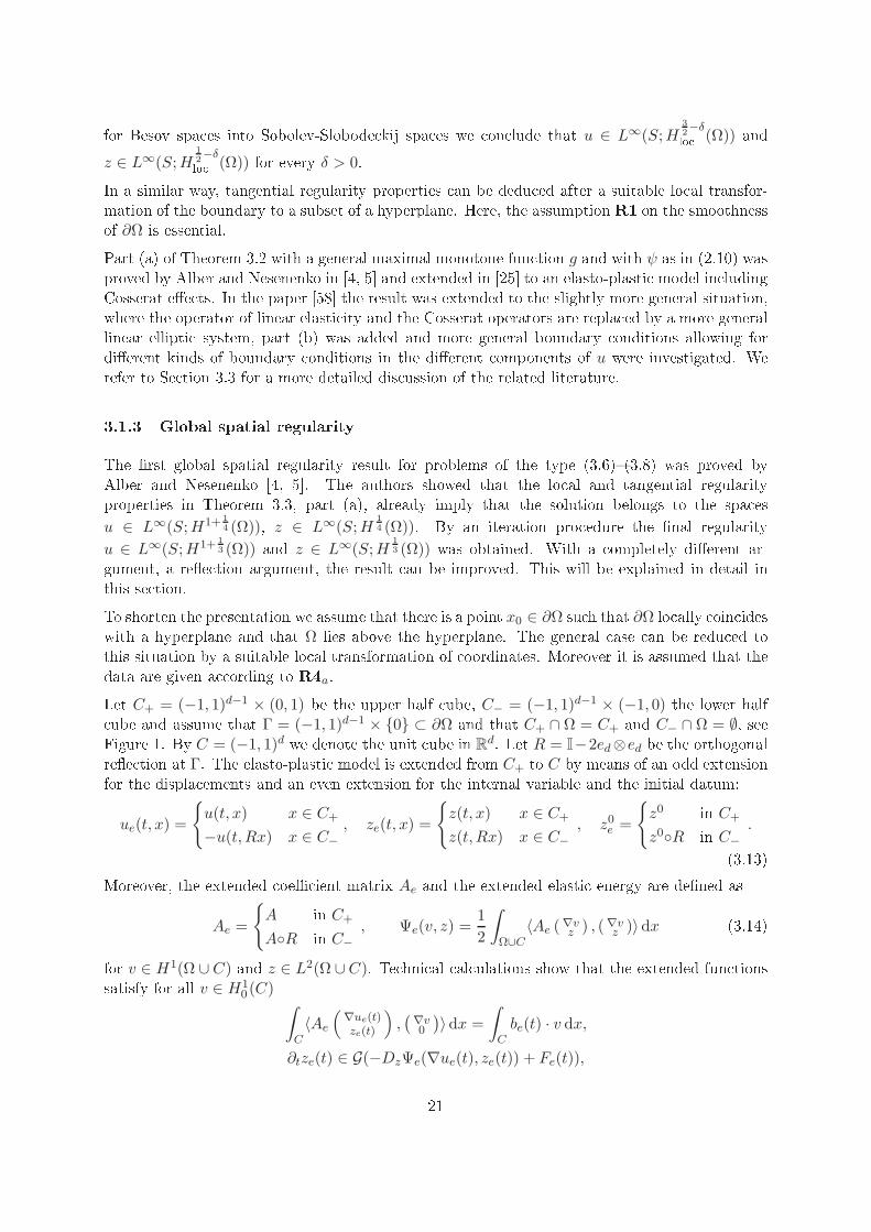
d. Let R = I−2ed⊗ed be the orthogonalree tion at Γ. The elasto-plasti model is extended from C+ to C by means of an odd extensionfor the displa ements and an even extension for the internal variable and the initial datum:ue(t, x) =

u(t, x) x ∈ C+

−u(t, Rx) x ∈ C−

, ze(t, x) =

z(t, x) x ∈ C+

z(t, Rx) x ∈ C−

, z0e =

z0 in C+

z0R in C−

.(3.13)Moreover, the extended oe ient matrix Ae and the extended elasti energy are dened asAe =

A in C+

AR in C−

, Ψe(v, z) =1

2

∫

Ω∪C〈Ae (∇v

z ) , (∇vz )〉dx (3.14)for v ∈ H1(Ω ∪C) and z ∈ L2(Ω ∪C). Te hni al al ulations show that the extended fun tionssatisfy for all v ∈ H1

0 (C)∫

C〈Ae

(∇ue(t)ze(t)

),(∇v0

)〉dx =

∫

Cbe(t) · v dx,

∂tze(t) ∈ G(−DzΨe(∇ue(t), ze(t)) + Fe(t)),21

wherebe(t, x) =

b(t, x) x ∈ C+

−b(t, Rx) − div((A11∇u(t) +A12z(t)

)∣∣Rx

(R+ I))

x ∈ C−, (3.15)

Fe(t, x) =

F (t, x) x ∈ C+

F (t, Rx) −A21,e(∇u(t)∣∣Rx

(R+ I)) x ∈ C−

. (3.16)The tangential regularity results from the previous se tion guarantee that be∣∣C−∈ L∞(S;L2(C−)).Indeed, due to the fa tor (R + I) terms like ∂2

du and ∂dz do not appear in the denition of beand hen e, tangential derivatives of ∇u and z enter in the denition of be, only, whi h, byTheorem 3.3, belong to L∞(S;L2(C−)). Again from the regularity results in the previous se -tion we obtain that ∂dFe

∣∣C±

∈ L∞(S;L2(C±)). Taking into a ount that u∣∣Γ

= 0, it followsthat ∇u(R + I)∣∣Γ

= 0 and hen e the tra es of Fe

∣∣C+

and Fe

∣∣C−

oin ide on Γ. This impliesthat ∂dFe ∈ L∞(S;L2(C)). The lo al regularity result des ribed in Theorem 3.3, part (b), istherefore appli able and leads to the following theorem:Theorem 3.4. Assume that R1R3 and R4a are satised. Then the unique solution (u, z) ofproblem (3.6)(3.8) satises: For every δ > 0

u ∈ L∞(S;H32−δ(Ω)) ∩ L∞(S;H2lo (Ω)), z ∈ L∞(S;H

12−δ(Ω)) ∩ L∞(S;H1lo (Ω)). (3.17)Moreover, for every δ > 0 there exists a onstant cδ > 0 su h that

‖u‖L∞(S;H

32−δ(Ω))

+ ‖z‖L∞(S;H

12−δ(Ω))

≤ cδ(∥∥z0

∥∥H1(Ω)

+ ‖f‖W 1,1(S;Y1)). (3.18)We refer to [58 for a detailed proof of the global results and a slightly more general variant ofTheorem 3.4, where also further types of boundary onditions are dis ussed.Estimates (3.9) and (3.18) allow to apply Tartar's nonlinear interpolation theorem showing thatfor data with less spatial regularity than required in Theorem 3.4, one obtains the orrespondingspatial regularity of the solution in a natural way. We assume here that g = ∂χK , where K ⊂ R

Nis onvex, losed and 0 ∈ K. ∂χK denotes the onvex subdierential of the hara teristi fun tion χK asso iated with K. Let Y0 := Q∗, Y1 := L2(Ω,Rm) × H1(Ω,RN ) and Qδ1 :=

(H10 (Ω,Rm) ∩ H 3

2−δ(Ω,Rm)) × H

12−δ(Ω,RN ) for δ > 0. Due to Theorem 3.1 and the stabilityestimate (3.9) for all r, q ∈ [1,∞] the solution operator T dened by

T : L2(Ω,RN ) ×W 1,r(S;Y0) → Lq(S;Q), (z0, f) 7→ T (z0, f) = (u, z),where (u, z) ∈ W 1,1(S;Q) is the unique solution of (3.6)(3.8) with data f = (b, F ) and initial ondition z0, is well dened and Lips hitz- ontinuous. Moreover, for all δ > 0 the solutionoperatorT : H1(Ω,RN ) ×W 1,r(S;Y1) → Lq(S;Qδ

1)is a bounded operator a ording to Theorem 3.4. Hen e, Tartar's interpolation Theorem [103,Thm. 1 guarantees that for all θ ∈ (0, 1) and all p ∈ [1,∞] the following impli ation holds true:z0 ∈ (H1(Ω);L2(Ω))θ,p, f ∈ (W 1,r(S;Y1);W

1,r(S;Y0))θ,p

=⇒ T (z0, f) = (u, z) ∈ (Lq(S;Qδ1);L

q(S;Q))θ,p.22

Here, (· ; ·)θ,p stands for real interpolation, see e.g. [107. If for example r = q = p = 2and θ ∈ (0, 1), then given z0 ∈ Hθ(Ω), b ∈ W 1,2(S; (H1−θ(Ω))∗), where Hs(Ω) = η ∈Hs(Ω) ; ∃η ∈ Hs(Rm) with supp η ⊂ Ω, η

∣∣Ω

= η , and F ∈ W 1,2(S;Hθ(Ω)) we obtain thatu ∈ L2(S;H1+θ( 1

2−δ)(Ω)) and z ∈ L2(S;Hθ( 1

2−δ)(Ω)).Example 3.5. Theorem 3.4 and the interpolation result are appli able to rate-independentelasto-plasti ity with linear kinemati hardening and with a von Mises or a Tres a ow rule.Here, the ve tor of internal variables is identied with the plasti strains εp ∈ R

d×dsym,dev (i.e.tr εp = 0) and the elasti energy takes the form

Ψ(u, εp) =

∫

Ωψ(ε(∇u), εp) dx with ψ(ε, εp) = 1

2A(ε− εp) · (ε− εp) + 12Lεp · εp, (3.19)for (ε, εp) ∈ R

d×dsym × Rd×dsym,dev. The oe ient tensors A ∈ C0,1(Ω,Lin(Rd×dsym,Rd×dsym)) and L ∈

C0,1(Ω,Lin(Rd×dsym,dev,Rd×dsym,dev)) are assumed to be symmetri and uniformly positive denite.Hen e, due to Korn's inequality, assumption R2 is satised. Let K ⊂ Rd×dsym,dev be onvex, losedand with 0 ∈ K. The set K des ribes the set of admissible stress states. Choosing g = ∂χK asthe onvex subdierential of the hara teristi fun tion χK asso iated with K, we obtain lassi alrate-independent models for elasto-plasti material behavior. In parti ular, the von Mises owrule is asso iated with the set KvM = τ ∈ R

d×dsym,dev ; (τ · τ) 12 ≤ c0 , whereas the Tres a owrule is based on the set KT = τ ∈ R

d×dsym,dev ; maxi6=j |τi − τj| ≤ c0 . Here, τi ; 1 ≤ i ≤ d are the eigenvalues (prin iple stresses) of τ ∈ Rd×dsym,dev. The regularity Theorem 3.4 and theinterpolation result are appli able to these models.Example 3.6. In [80 an elasti -plasti model was introdu ed whi h in orporates Cosserat mi- ropolar ee ts. This model is analyzed in [80, 25 with respe t to existen e and lo al regularityand in [59 with respe t to global regularity of a time dis retized version. In this model, notonly the displa ements u but also linearized mi ro-rotations Q are taken into a ount. The gen-eralized displa ements are given by the pair (u,Q) ∈ R

d × Rd×dskew ∼= R

m, whereas the internalvariable z is identied with the plasti strain tensor z = εp ∈ Rd×dsym, dev. For u ∈ H1(Ω,Rd),

Q ∈ H1(Ω,Rd×dskew) and εp ∈ L2(Ω,Rd×dsym,dev) the elasti energy readsΨC((u,Q), εp) =

∫

Ωµ |ε(∇u) − εp|2 + µc |skew (∇u−Q)|2 +

λ

2|tr∇u|2 + γ |∇Q|2 dx.Here, λ, µ > 0 are the Lamé onstants, µc > 0 is the Cosserat ouple modulus and γ > 0depends on the Lamé onstants and a further internal length parameter. It is shown in [80 that

ΨC satises ondition R2. If G is hosen a ording to R3, then solutions to (3.6)(3.8) with ΨChave the global regularity properties des ribed in Theorem 3.4. In addition, Q ∈ L∞(S;H2(Ω)),sin e Q is oupled with ε(∇u) and εp through lower order terms, only, see [25.3.2 Dis ussion of the regularity resultsIt is an unsolved problem whether the result in Theorem 3.4 is optimal or whether one shouldexpe t the regularity u ∈ L∞(S;H2(Ω)), z ∈ L∞(S;H1(Ω)) for domains with smooth bound-aries. This would extend the lo al regularity results des ribed in Theorem 3.3 in a natural way.If u is a s alar fun tion, then under ertain oupling onditions on the oe ients the spatialregularity u ∈ L∞(S;H2(Ω)) an be a hieved for the evolution model (see Se tion 3.2.1). InSe tion 3.2.2 we give an example whi h shows that in spite of smooth data a similar regularityresult is not valid for the time derivatives ∂tu and ∂tz.23

3.2.1 Improved regularity for s alar uThe regularity results in Theorem 3.4 an be improved if u is s alar and if ertain ompatibility onditions between the submatri es Aij of A and the onstitutive fun tion g are satised. Herethe idea is to onstru t a ree tion operator R, whi h is adapted to the stru ture of the the oe ient matrix A11. In ontrast to Se tion 3.1.3 the problem is not ree ted perpendi ularto the boundary but with respe t to the ve tor A11ν, where ν : ∂Ω → ∂B1(0) ⊂ Rd is theinterior normal ve tor to ∂Ω. Due to the ompatibility onditions between the oe ients andthe onstitutive fun tion g the ree ted data do not ontain se ond spatial derivatives of u orrst derivatives of z. Hen e the ree ted data have the regularity (be, Fe) ∈W 1,1(S;Y1) insteadof (be, Fe) ∈ L∞(S;Y1) with Y1 = L2(Ωe) ×H1(Ωe). Thus, we may apply part (a) of Theorem3.3 and obtain the improved global regularity des ribed in Theorem 3.7 here below.To be more pre ise, the problem under onsideration reads: Find u : S × Ω → R, z : S ×

Ω → RN su h that for given A11 ∈ C0,1(Ω,Rd×dsym), A12 = A⊤

21 ∈ C0,1(Ω,Lin(RN ,Rd)) andA22 ∈ C0,1(Ω,RN×Nsym ) we have

DuΨ(u(t))[v] =

∫

Ω(A11∇u(t) +A12z(t)) · ∇v dx =

∫

Ωb(t) · v dx ∀v ∈ V,

∂tz(t) ∈ G(−(A21∇u(t) +A22z(t)) + F (t)),

z(0) = z0.It is assumed that A =(

A11 A12A21 A22

)∈ C0,1(Ω; R(d+N)×(d+N)) is uniformly positive denite. Let

ν : ∂Ω → ∂B1(0) be the interior normal ve tor on ∂Ω. In order to formulate the ompatibility onditions, we dene for x ∈ ∂Ω

Rν(x) = I − 2

A11(x)ν(x) · ν(x)A11(x)ν(x) ⊗ ν(x). (3.20)The matrix Rν lo ally determines the ree tion at ∂Ω. Simple al ulations show that R2

ν(x) = Iand Rν(x)A11(x)R⊤ν(x) = A11(x). The basi assumptions and ompatibility onditions are:R5 Ω ⊂ R

d is a bounded domain with a C2,1-smooth boundary (it is used that ν ∈ C1,1(∂Ω)).R6 (b, F ) ∈W 1,1(S;Y1) with Y1 from R4a, z0 = 0.R7 There exists a mapping P ∈ C0,1(∂Ω,RN×N ) su h that for every x ∈ ∂Ω the inverse matrix(P (x))−1 exists and the following onditions hold for all η ∈ R

N

Rν(x)A12(x)P (x) = A12(x), P (x)⊤A22(x)P (x) = A22(x), −P (x)−1g(−P (x)−⊤η) = g(η).Theorem 3.7. [58 Let R5-R7 be satised and assume that the pair (u, z) ∈ W 1,1(S;H10 (Ω) ×

L2(Ω)) solves (3.6)(3.8). Then u ∈ L∞(S;H2(Ω)) and z ∈ L∞(S;H1(Ω)).We refer to [58 for a detailed proof.Example 3.8. Assume that the oe ient matrix A is onstant, that N = d, A12 = −A11 andA22 = A11 + L with L ∈ R

d×dsym positive denite. Hen e, Ψ(u, z)= 12

∫ΩA11(∇u − z) ·(∇u − z)+

Lz · zdx. Moreover we assume that A11=I, whi h an always be a hieved after a suitable hangeof oordinates and a suitable transformation in the state spa e of z. The mapping Rν now takesthe form Rν = I − 2ν ⊗ ν for ν ∈ ∂B1(0) and the ompatibility onditions redu e to24

R7' Pν = Rν , R⊤ν LRν = L and −R⊤

ν g(−Rνη) = g(η) for all η ∈ Rd.It is shown in [58 that R7' is satised if and only if there exists α > 0 su h that L = αI.Moreover, if g = ∂χK with K ⊂ R

d onvex, losed and 0 ∈ K, then R7' holds if and only ifK = −RνK for all ν ∈ R

d. In this situation, Theorem 3.7 yields the improved regularity result.This example shows that if the anisotropy in Hooke's law given by the matrix A11 is orrelatedwith the anisotropy in the hardening oe ients A22 and L and the onstitutive fun tion g, thenthe displa ements u(t) have full H2-regularity up to the boundary ∂Ω. It is an open questionwhether this regularity is still valid if the ompatibility ondition R7 is violated. Moreover it isnot known, whether a similar result is true for real elasto-plasti models, where u is not a s alarfun tion.3.2.2 Example: ∂tz(t) /∈ H1(Ω)The following example shows that in spite of smooth data there might exist a time interval (t1, t2)su h that ∂tz(t) /∈ H1(Ω) for all t ∈ (t1, t2). Hen e, one should not expe t z ∈ W 1,1(S;H1(Ω)).The example is inspired by Seregin's paper [95.Let 0 < R1 < R2. We set Ω = BR2(0)\BR1(0) and hoose the following energy for u, z : Ω → R:Ψ(u, z) = 1

2

∫

Ω

∣∣∇u− x|x|z

∣∣2 + z2 dx.Moreover, g(η) := ∂χ[−1,1](η) for η ∈ R. It is assumed that u(t)∣∣∂BR1

= 0, u(t)∣∣∂BR2

= t,z0 = 0 and that the remaining data (F , b) vanish. It is easily he ked that the assumptionsof Theorem 3.7 are satised and hen e the problem has a unique solution with the regularity∇u, z ∈ W 1,1(S;L2(Ω)) ∩ L∞(S;H1(Ω)). Due to the rotational symmetry of the problem thesolution does not depend on the angle and an be al ulated expli itly. Introdu ing polar- oordinates, the solution u, z : S × (R1, R2) → R has to satisfy for r ∈ (R1, R2) and t ∈ S

∂2ru+ r−1∂ru− ∂rz − r−1z = 0 in S × (R1, R2),

∂tz ∈ ∂χ[−1,1](∂ru− 2z) in S × (R1, R2),

z(0, ·) = 0, u(t, R1) = 0, u(t, R2) = t.For t ≤ t1 := R1 ln(R2/R1) it follows that u(t, r) = t ln(r/R1)ln(R2/R1) , z(t, r) = 0. In this regime, noplasti strains are present. For t > t1 the plasti variable z starts to grow and there exists r∗(t)su h that z(t, r) > 0 for r < r∗ and z(r, t) = 0 for r > r∗, i.e. r∗(t) separates the plasti regionfrom the elasti region. The dependen e of r∗ on t is given impli itly by the relation

t(r∗) = R1 − r∗ + r∗(lnR2r∗ − lnR21).Simple al ulations show that t(r∗) is stri tly in reasing, and hen e r∗(t) ≥ R1 is stri tly growing,as well. Moreover, for t ≥ t1 we have

u(t, r) =

b(t) − r + 2r∗(t) ln r if r ≤ r∗(t)

c(t) + r∗(t) ln r else , z(t, r) =

−1 + r∗(t)r

−1 if r ≤ r∗(t),

0 else ,with fun tions b(t) = R1 − 2r∗(t) lnR1 and c(t) = t− r∗(t) lnR2. Sin e ∂tr∗(t) > 0 for t ≥ t1 itfollows that ∂tz(t, ·) /∈ H1(R1, R2) for t > t1, see also Figure 1.25

PSfrag repla ementsΩ

C+

C−

xdx′

z ∂tz

Figure 1: Example for the notation in Se tion 3.1.3 (left); Graph of the solution z : (0, T ) ×(R1, R2) → R (middle) and of the time derivative ∂tz (right).3.3 Regularity for variants of the elasto-plasti model and overview on the orresponding literatureThe starting point for the review of the literature on spatial regularity properties of elasto-plasti models is the system introdu ed in (3.6)(3.8) with the parti ular energy density

ψ(ε, z) = 12

(A(ε−Bz) · (ε−Bz) + Lz · z

) (3.21)for ε ∈ Rd×dsym and z ∈ R

N . It is assumed that A ∈ Lin(Rd×dsym,Rd×dsym) is symmetri and positivedenite, L ∈ Lin(RN ,RN ) is symmetri and positive semi-denite and B ∈ Lin(RN ,Rd×dsym). The orresponding evolution model readsdiv σ(t) + b(t) = 0, σ(t) = A(ε(∇u(t)) −Bz(t)), (3.22)

∂tz(t) ∈ G(−∂zψ(ε(∇u(t)), z(t)) + F (t)). (3.23)together with initial and boundary onditions. Depending on the properties of L and G dierentspatial regularity results were derived in the literature.3.3.1 Regularity for models with positive semi-denite elasti energy and mono-tone, multivalued gOnly very few regularity results are available for models where the elasti energy density ψ in(3.21) is positive semi-denite but not positive denite. The orresponding elasti energy is on-vex but not stri tly onvex on the full state spa e Q. As a onsequen e, a-priori estimates likethose provided in Theorem 3.2 annot be obtained in general. In ontrast, the omplementaryenergy, whi h is expressed via the generalized stresses, is still oer ive. The regularity investi-gations therefore typi ally take a stress based version of (3.22)(3.23) as a starting point. Inthis framework to the authors' knowledge only the Prandtl-Reuss model and models with linearisotropi hardening are dis ussed in the literature with regard to regularity questions.The Prandtl-Reuss model des ribes elasti , perfe tly plasti material behavior without hardening.The internal variable z is identied with the plasti strain tensor εp ∈ Rd×dsym,dev, B = I and L = 0.Moreover, the onstitutive fun tion g is typi ally identied with ∂χK , where K is a onvex setgiven a ording to the von Mises or the Tres a ow rule, see Example 3.5.The existen e theorems provide stresses with σ(t) ∈ L2(Ω) and u(t) ∈ BD(Ω), where BD(Ω)denotes the spa e of bounded deformations, see e.g. [53, 67, 102, 8, 105, 28. Higher spatialregularity is derived by Bensoussan and Frehse [13 and Demyanov [31 for the ase that K isdened by the von Mises yield ondition. They obtain σ ∈ L∞([0, T ];H1lo (Ω)), whi h oin ides26

with the lo al results in Theorem 3.4. The stress regularity is proved by approximating thePrandtl-Reuss model with the vis ous power-law like Norton-Ho model [13 and by time dis- retization [31. Tangential properties are dis ussed in [18. To the author's knowledge theseare the only known spatial regularity results for the Prandtl-Reuss model. In parti ular there isno information about higher global regularity. In the dynami al ase, Shi proved a lo al spatialresult for σ and u [96.If z(0) = 0, then the rst step in the time dis retization of the Prandtl-Reuss model leads to thestationary, elasti , perfe tly plasti Hen ky model. Here, it is proved for the von Mises ase thatσ ∈ H1lo (Ω)∩H 1

2−δ(Ω) for every δ > 0, where Ω is a bounded Lips hitz domain whi h satises anadditional geometri al ondition near those points, where the Diri hlet and Neumann boundaryinterse t. We refer to [12 and [92, 39 together with the referen es therein for the lo al resultand to [56, 15 for the global and a tangential result. The key of the proofs is to approximatethe Hen ky model with nonlinear elasti models and to derive uniform regularity estimates forthe approximating models. In addition, the authors in [39 obtain a result on erning partialregularity of the solutions. It is an open problem whether the global result an be improved in the ase of a smooth boundary with pure Diri hlet or pure Neumann onditions, see the dis ussionin [95.A further typi al elasto-plasti model with a positive semidenite energy density ψ des ribeslinear isotropi hardening. Here, the internal variable z onsists of the plasti strains εp and as alar hardening variable γ hara terizing the radius of the set of admissible stress states. Thequadrati elasti energy is given by ψ(ε, εp, γ) = 1

2

(A(ε − εp) · (ε − εp) + αγ2

) for ε ∈ Rd×dsym,

εp ∈ Rd×dsym,dev and xed α > 0. The onstitutive fun tion is dened as g = ∂χK with K =

(τ, µ) ∈ Rd×dsym,dev × R ; µ ≥ 0, |τ | ≤ σ0 + σ1µ and onstants σi > 0. The rst investigations on erning spatial regularity in the isotropi ase were arried out by Seregin [93. Here, theresults σ ∈ L∞(S;H1lo (Ω)), γ ∈ L∞(S;H1lo (Ω)), ∇u ∈ L∞(S;BDlo (Ω)) were obtained bystudying the regularity properties of a time-dis retized version and proving uniform bounds.Hölder properties of the solutions were investigated in [37.3.3.2 Spatial regularity for regularized modelsRepla ing the maximal monotone onstitutive fun tion G : L2(Ω,RN ) → P(L2(Ω,RN )) from(3.23) with its Yosida approximation leads to regularized elasto-vis o-plasti models with aLips hitz- ontinuous nonlinearity in the evolution law. The therewith obtained models are asub lass of the elasto-vis o-plasti models studied e.g. by Sofonea et al., see [52, 35. Given anenergy Ψ : Q → R as dened in (3.4)(3.5) with a oe ient matrix A ∈ L∞(Ω,Lin(Rm×d ×

RN ,Rm×d × R

N )) and given a Lips hitz- ontinuous operator F : Q → L2(Ω,RN ) these modelsread as follows:DuΨ(u(t), z(t)) = b(t), ∂tz(t) = F(u(t), z(t)), z(0) = z0 (3.24)together with boundary onditions on ∂Ω. If the submatrix A11 ∈ L∞(Ω,Lin(Rm×d,Rm×d)) of

A is symmetri and if the indu ed bilinear form a(u, v) =∫ΩA11∇u · ∇v dx is oer ive on V ,then a standard appli ation of Bana h's xed point theorem implies the existen e of a uniquesolution (u, z) ∈W 1,∞(S;Q) provided that b ∈W 1,∞(S;V ∗).For these models the lo al spatial regularity was investigated in [75 with a dieren e quotientargument and in [61, while the global regularity was studied in [19. The global regularity the-orem in [19 states that if the linear ellipti operator indu ed by A11 is an isomorphism between27

the spa es H1ΓDir(Ω) ∩ H1+s(Ω) and Ys for some s ∈ (0, 1], where Ys is a suitable subspa e of

Hs−1(Ω), then for every b ∈ W 1,∞(S;Ys) the solution of (3.24) satises u ∈ W 1,∞(S;H1+s(Ω))and z ∈ W 1,∞(S;Hs(Ω)). In this way, global regularity properties of ellipti operators on pos-sibly nonsmooth domains and with mixed boundary onditions dire tly inuen e the regularityproperties of the vis ous evolution model (3.24). The proof is arried out by deriving uniformregularity bounds for the sequen e of approximating solutions generated via the Bana h xedpoint theorem. Here it is not needed that the elasti energy Ψ is oer ive on Q, the oer ivityof a(u, v) :=∫ΩA11∇u · ∇v dx on V is su ient.While for elasto-plasti ity models (with a multivalued monotone onstitutive fun tion g) lo alregularity results an be dedu ed by proving uniform regularity bounds for the sequen e of theapproximating Yosida-regularized models, see e.g. [5, it is an unsolved problem, how to obtainuniform bounds in order to arry over global spatial regularity results from the vis ous model tothe elasto-plasti limit problem.A further possibility to regularize elasto-plasti models is to repla e the onstitutive fun tion

G = ∂χK with a power-law like ansatz. This approa h is used in [105 in order to regularize thePrandtl-Reuss model. Assume again that z = εp ∈ Rd×dsym,dev, B = I, L = 0 and repla e ∂χKvM( f. Example 3.5) with

gN (σ) = c1−N0

∣∣σD∣∣N−2

σD,for σ ∈ Rd×dsym. Here, σD = σ− 1

d tr σ I denotes the deviatori part of the tensor σ. The parameterN > 1 is a strain hardening exponent, whereas c0 an be interpreted as a yield stress. Theresulting vis ous model is the so alled Norton/Ho model and onsists of the relation (3.22)whi h is ompleted by the evolution law ∂tεp(t) = gN (σ(t)). For N → ∞, the Norton/Homodel approximates the Prandtl/Reuss model [105. After eliminating the plasti strains εp oneobtains the usual form of the Norton/Ho model:

div σ(t) + b(t) = 0, A−1∂tσ(t) + c1−N0

∣∣σD(t)∣∣N−2

σD(t) = ∂tε(∇u(t)).Bensoussan/Frehse [12 proved the lo al spatial regularity result σ ∈ L∞((0, T );H1lo (Ω)) for thestress tensor via a dieren e quotient argument. A global result seems not to be available in theliterature.A time dis retization of the Norton/Ho model leads to the stationary Norton/Ho or Ram-berg/Osgood model, whi h is given by equation (3.22) in ombination with the relation ε(∇u) =

A−1σ + c1−N0

∣∣σD∣∣N−2

σD. Several authors studied lo al and global regularity and the Hölderproperties of the stresses and displa ements of this model for domains with smooth boundariesas well as for domains with nonsmooth boundaries [12, 101, 55, 56, 14, 33.3.3.3 Spatial regularity for time in remental versionsA further way to prove regularity properties of elasto-vis oplasti models is to study the smooth-ness of solutions to time-dis retized versions and to derive regularity bounds whi h are uniformwith respe t to the time step size. This method was applied e.g. in [93 to obtain lo al results,while for global results uniform bounds are not known. We dis uss here global regularity prop-erties for the time dis retized version under the assumption that the elasti energy Ψ is oer iveand that g = ∂χK with a onvex and losed set K. The dierent equivalent formulations of28

the dis retized equations, whi h we present here below, are ommonly used in a omputational ontext of elasto-plasti ity, [99, 98.Let R1 and R2 be satised and assume that g = ∂χK , where K ⊂ RN is onvex, losed and with

0 ∈ K. Let further K = η ∈ L2(Ω) ; η(x) ∈ K a.e. in Ω . A time dis retization via an impli itEuler s heme leads to the following problem with ∆t = T/n, 0 = tn0 < tn1 < . . . < tnn = T : Find(un

k , znk ) ∈ V × L2(Ω), 1 ≤ k ≤ n, whi h satisfy

DuΨ(unk , z

nk ) − b(tnk ) = 0, 1

∆t(znk − zn

k−1) ∈ ∂χK(−DzΨ(unk , z

nk )). (3.25)Observe that zn

k solves (3.25) if and only ifznk = argminF (un

k , η, znk−1,∆t) ; η ∈ L2(Ω) , (3.26)

F (unk , η, z

nk−1,∆t) =

1

2

∫

ΩA22(η − zk−1) · (η − zk−1) dx+ ∆t χK(−(A21∇un

k +A22znk )). (3.27)In terms of the new variables Σtrial

k = −(A21∇unk + A22z

nk−1) and Σk = −(A21∇un

k + A22znk ), itfollows that zk satises (3.26) if and only if

znk = zn

k−1 +A−122 (Σtrial

k − Σk), (3.28)Σk = argmin F (θ,Σtrial

k ,∆t) ; θ ∈ L2(Ω) , (3.29)F (θ,Σtrial

k ,∆t) =1

2

∫

ΩA−1

22 (θ − Σtrialk ) · (θ − Σtrial

k ) dx+ ∆t χK(θ). (3.30)Sin e the oe ient matrix A−122 indu es a s alar produ t on L2(Ω), Σk an be interpreted asthe proje tion of Σtrial

k onto the onvex and losed set K with respe t to this s alar produ t. LetPA−1

22 ,K : L2(Ω) → L2(Ω) be the proje tion operator on K. Hen e, Σk = PA−122 ,K(Σtrial

k ) and inaddition, Σk(x) = PA−122 (x),K(Σtrial

k (x)) in Ω, where PA−122 (x),K : R

N → RN is the orrespondingpointwise proje tion operator on K. With these notations, problem (3.25) is equivalent to thefollowing problem: Find un

k ∈ V and znk ∈ L2(Ω) su h that for given zn

k−1 ∈ L2(Ω) we have∫

ΩM(x,∇un

k (x), znk−1(x)) · ∇v(x) dx = 〈b(tnk), v〉 ∀v ∈ V, (3.31)

znk = −A−1

22

(A21∇un

k + PA−122 ,K( −A21∇un

k −A22znk−1)

), (3.32)where the mapping M : Ω × R

m×d × RN → R

m×d is dened asM(x, F, z) = L1(x)F −A12(x)A22(x)

−1PA−122 (x),K

(−A21(x)F −A22(x)z

)with the S hur omplement matrix L1 = A11−A12A−122 A21 ∈ C0,1(Ω,Lin(Rm×d,Rm×d)). Observethat in general M is not dierentiable with respe t to F and z. The Lips hitz- ontinuity of theproje tion operator, assumption R2 and the assumption 0 ∈ K imply that the mapping Mhas the following properties: there exist onstants c1, c2 > 0 su h that for every x, xi ∈ Ω,

F,Fi ∈ Rm×d and z, zi ∈ R

N we have|M(x1, F, z) −M(x2, F, z)| ≤ c1(|F | + |z|) |x1 − x2| , (3.33)

|M(x, F1, z1) −M(x, F2, z2)| ≤ c2(|F1 − F2| + |z1 − z2|), (3.34)M(x, 0, 0) = 0. (3.35)29

Moreover, M indu es a strongly monotone operator on V , i.e. there exists a onstant β > 0 su hthat for all u1, u2 ∈ V and z ∈ L2(Ω) we have:∫

Ω

(M(x,∇u1, z) −M(x,∇u2, z)

): ∇(u1 − u2) dx ≥ β ‖u1 − u2‖2

H1(Ω) .This follows from the monotoni ity of the proje tion operator and from the fa t that due toassumption R2, the indu ed bilinear form b(u, v) :=∫Ω L1∇u · ∇v dx, u, v ∈ V , is symmetri and V - oer ive. Finally, the mapping M is strongly rank-one monotone. That means that thereexists a onstant cLH > 0 su h that for every x ∈ Ω, F ∈ R

m×d, z ∈ RN , ξ ∈ R

m and η ∈ Rd wehave

(M(x, F + ξ ⊗ η, z) −M(x, F, z)) : ξ ⊗ η ≥ cLH |ξ|2 |η|2 . (3.36)This is a onsequen e of the monotoni ity of the pointwise proje tion operator and the positivityproperties of L1, see e.g. [108, Th. 6.1. Altogether it follows that M generates a quasilinearellipti system of PDEs of se ond order for determining un

k . Standard existen e results forequations involving Lips hitz- ontinuous, strongly monotone operators guarantee the existen eof a unique element unk ∈ V solving (3.31) for arbitrary data zn

k−1 ∈ L2(Ω) and b ∈ V ∗, [110.Moreover, unk depends Lips hitz- ontinuously on the data. The regularity result in [59 guaranteesthat for given b(tk) ∈ L2(Ω) and zn

k−1 ∈ H1(Ω) we have the global regularity (unk , z

nk ) ∈ H2(Ω)×

H1(Ω) provided that R1 and R2 are satised. Unfortunately it is not known how to deriveestimates for ‖unk‖H2(Ω) whi h are uniform with respe t to the time step ∆t.Quasilinear ellipti systems of a similar stru ture resulting from various regularizing ansatzesfor elasto-plasti models were also studied with respe t to regularity questions in the referen es[86, 20, 57, 91, 94, 38, 79, 89.4 Numeri al realization via a Slant Newton MethodAs it is pointed out in Se tion 3.3.3 one possibility to numeri ally solve the system of elasto-plasti ity is to solve the system of nonlinear ellipti equations whi h emerges after an (impli it)time dis retization and an elimination of the internal variables. This system in general involves anonlinearity whi h is not dierentiable as an operator between fun tion spa es. Hen e, a standardNewton's method, whi h relies on the derivative of the nonlinear operator, is not appropriate tosolve the nonlinear system. Instead we dis uss a Newton-like method, where the derivative isrepla ed by a slanting fun tion leading to a Slant Newton Method. This approa h is explainedfor a rate-independent elasto-plasti model with linear isotropi hardening.4.1 Problem Spe i ationConsider the Prandtl-Reuÿ elastoplasti ity problem with isotropi hardening, whi h is a spe ial-ization of (2.1)(2.5) in the following way: Dene the internal variable with size N = 7 via

z(x, t) = (z1(x, t), . . . , z6(x, t), γ(x, t)), and the proje tionB : R

N → S3 , z 7→ εp =

z1 z4 z5z4 z2 z6z5 z6 z3

. (4.1)30

For easier notation let us, from now on, denote the plasti strain by p instead of εp. Theasso iated free energy density is assumed to be of the formψ(ε, p, γ) =

1

2〈A(ε− p), ε− p〉F +

1

2γ2 ,where ε ∈ S3, p ∈ S3, γ ∈ R, the Frobenius s alar produ t for matri es is dened 〈B,C〉F =∑

ij Bij Cij, and it is assumed that the elasti ity tensor A hara terizes isotropi material be-havior and has the expli it formA : S3 → S3, ε 7→ 2µε+ λ tr ε I .Here, λ, µ > 0 are the Lamé onstants and des ribe the elasti behavior of the material. This hoi e of the elasti energy density indu es the following relation between the generalized plasti strains Π = (p, γ) ∈ S3 × R and the generalized stresses Σ = (T, α) ∈ S3 × R:

T = ∂εψ(ε, p, γ) = −∂pψ(ε, p, γ) = A(ε− p) ,

α = −∂γψ(ε, p, γ) = −γ .The onstitutive ow law (2.3) in the Prandtl-Reuss ase with isotropi hardening reads∂tΠ(x, t) ∈ ∂χK(Σ(x, t)) , (4.2)where ∂χK denotes the subgradient of the indi ator fun tion regarding the onvex set K ofadmissible generalized stresses, whi h is given by

K = Σ ∈ S3 × R ; φ(Σ) ≤ 0 (4.3)with the yield fun tionφ(Σ) = ‖dev T‖F − Ty(1 +Hα) + χ[0,∞)(α). (4.4)The parameters yield stress Ty > 0 and modulus of hardening H > 0 des ribe the plasti behaviorof the material, the deviator, a proje tion onto the tra e-free subspa e of S3, is al ulated by

dev T = T − (tr T/ tr I) I, and the Frobenius norm reads ‖T‖2F = 〈T, T 〉F . Noti e, that (4.2)is a spe ialization of (2.3). Geometri ally spoken, the subgradient ∂χK des ribes the normal one of the onvex set of admissible stresses K at the point Σ. In other words, the pres ription

∂Π∂t ∈ ∂χK(Σ) means that either there is no solution with respe t to the generalized strain Π (ifΣ is not in K), or Π remains onstant (if Σ is in the interior of K), or ∂Π

∂t has to be hosen su hthat it is orthogonal to the boundary of the set of admissible stresses K at the point Σ (if Σ ison the boundary of K).Summarizing, the problem of Prandtl-Reuÿ elastoplasti ity with isotropi hardening reads: Findthe displa ement u(x, t) ∈ R3, the plasti strain p(x, t) ∈ S3, and the hardening parameter

α(x, t) ∈ R, whi h solve− divx T (x, t) = b(x, t) , (4.5)

T (x, t) = A(ε(u(x, t)) − p(x, t)) , (4.6)∂ Π

∂t(x, t) ∈ ∂χK(Σ(x, t)) , where Π = (p,−α) and Σ = (T, α) , (4.7)

Π(x, 0) = Π(0)(x) , (4.8)u(x, t) = γD(x, t) , if x ∈ ΓD ⊂ ∂Ω , (4.9)

T (x, t)n(x, t) = γN (x, t) , if x ∈ ΓN ⊂ ∂Ω . (4.10)31

We turn to the numeri al solution of the problem (4.5)(4.10). The algorithm des ribed in thisse tion is of Newton's type, enjoying the property of lo al super-linear onvergen e. It is aninteresting question for future investigation, whether there is a more general lass of problems overed by the laws (2.1)(2.5), to whi h this algorithm is appli able.We dene V :=[H1(Ω)

]3, V0 := v ∈ V ; v = 0 on ΓD , VD := v ∈ V ; v = uD on ΓD foruD ∈

[H1/2(ΓD)

]3, Q :=[L2(Ω,S3)

], and R := R ∪ +∞.Analogously to the dis ussion in Se tion 5 the problem (4.5)(4.10) may equivalently be formu-lated in the global energeti framework based on the energyE(t, u,Π) =

∫

Ωψ(ε(∇u), p, γ) dx − 〈b(t), u〉and the dissipation potential

R(u, p, γ) =

∫

Ωρ(p(x), γ(x)) dxfor u ∈ VD, p ∈ Q and γ ∈ L2(Ω). The density ρ is given as the onvex onjugate of χK and hasthe stru ture

ρ(p, γ) = χ∗K(p, γ) =

Ty ‖p‖F if tr p = 0 and ‖p‖F ≤ − γ

TyH ,

∞ otherwise .Using an impli it Euler-dis retization for a partition 0 = t0 < t1 < . . . < tn = T and the setsL2

+(Ω) = f ∈ L2(Ω) ; f ≥ 0 almost everywhere ,L2−(Ω) = f ∈ L2(Ω) ; f ≤ 0 almost everywhere ,the time dis retized problem reads:Problem 4.1. Given (uk−1, pk−1, γk−1) ∈ VD ×Q× L2

−(Ω) nd (uk, pk, γk) ∈ VD ×Q× L2−(Ω)su h that

(uk, pk, γk) ∈ argmin E(tk, v, q, ξ) + R(v − uk−1, q − pk−1, ξ − γk−1) ; (v, q, ξ) ∈ VD ×Q× L2−(Ω) .It is shown in [21, 6 that the hardening variable αk = −γk an be eliminated from the min-imization problem in su h a way that for determining (uk, pk,−αk) one an equivalently solvethe following problem:Problem 4.2. Given (uk−1, pk−1, αk−1) ∈ VD ×Q×L2

+(Ω) nd (uk, pk, αk) ∈ VD ×Q×L2+(Ω)su h that

(uk, pk) ∈ argmin Jk(v, θ) ; (v, θ) ∈ VD ×Q , (4.11)αk = αk−1 + TyH ‖pk − pk−1‖F . (4.12)Here, the global energy fun tional Jk : VD ×Q→ R is dened by

Jk(v, q) :=1

2‖ε(v) − q‖2

A + ψk(q) − lk(v) , (4.13)32

with〈q1, q2〉A :=

∫

Ω〈Aq1(x) , q2(x)〉F dx , ‖q‖A := 〈q, q〉1/2

A , (4.14)αk(q) := αk−1 + TyH‖q − pk−1‖F , (4.15)ψk(q) :=

∫Ω

(12 αk(q)

2 + Ty‖q − pk−1‖F

)dx if tr q = tr pk−1 ,

+∞ else , (4.16)lk(v) :=

∫

Ωbk · v dx+

∫

ΓN

γN,k · v ds . (4.17)The body for e b(tk) = bk ∈[L2(Ω)

]3 and the tra tion γN (tk) = γN,k ∈[H−1/2(ΓN )

]3 are given.The fun tional Jk expresses the me hani al energy of the deformed system at the kth time step.Noti e, that Jk is smooth with respe t to the displa ements v, but not with respe t to the plasti strains q.4.2 Solver AnalysisIn [21 a method of an alternate minimization regarding the displa ement v and the plasti strainq was investigated to solve Problem 4.2. The global linear onvergen e of the resulting methodwas shown and a lo al super-linear onvergen e was onje tured. Another interesting te hniqueis to redu e Problem 4.2 to a minimization problem with respe t to the displa ements v only.This an be a hieved by substituting the known expli it minimizer of Jk with respe t to theplasti strain eld for some given displa ement v, namely by q = pk(ε(v)). We will observethat su h a redu ed minimization problem is smooth with respe t to the displa ements v and itsderivative is expli itly omputable.The following theorem is formulated for fun tionals mapping from a Hilbert spa e H providedwith the s alar produ t 〈, ⋄〉H and the norm ‖·‖2

H:= 〈·, ·〉H. If a fun tion F is Fré het dieren-tiable, we shall denote its derivative in a point x by DF (x) and its Gâteaux dierential in thedire tion y by DF (x ; y). We refer to [34 on erning the denitions of onvex, proper, lowersemi- ontinuous, and oer ive.Theorem 4.3. Let the fun tion f : H × H → R be dened

f(x, y) =1

2‖x− y‖2

H + ψ(x) (4.18)where ψ is a onvex, proper, lower semi- ontinuous, and oer ive fun tion of H into R. ThenF (y) := infx∈H f(x, y) maps into R, and there exists a unique fun tion x : H → H su h thatF (y) = f(x(y), y) for all y ∈ H. Moreover, it holds:1. F is stri tly onvex and ontinuous in H.2. F is Fré het dierentiable with the Fré het derivative

DF (y) = 〈y − x(y) , ·〉H for all y ∈ H . (4.19)Proof. See [77, 7.d. Proposition.We apply Theorem 4.3 to Problem 4.2 and obtain the following proposition.33

Proposition 4.4. Let k ∈ 1, . . . , n denote the time step, and let Jk be dened as in (4.13).Then there exists a unique mapping pk : Q→ Q satisfyingJk (v, pk (ε (v))) = inf

q∈QJk (v, q) ∀v ∈ VD . (4.20)Let Jk be a mapping of VD into R dened as

Jk(v) := Jk(v, pk(ε(v))) ∀v ∈ VD . (4.21)Then, Jk is stri tly onvex and Fré het dierentiable. The asso iated Gâteaux dierential readsDJk(v ; w) = 〈ε(v) − pk(ε(v)) , ε(w)〉A − lk(w) ∀w ∈ V0 (4.22)with the s alar produ t 〈, ⋄〉A dened in (4.14) and lk dened in (4.17).Proof. The fun tional Jk : V × Q → R dened in (4.13) using (4.14), (4.16) and (4.17) an bede omposed in Jk(v, q) = fk(ε(v), q)−lk(v), where the fun tional fk : Q×Q→ R reads fk(s, q) :=

12‖q − s‖2

A + ψk(q). Theorem 4.3 states the existen e of a unique minimizer pk : Q → Q whi hsatises the ondition fk(s, pk(s)) = infq∈Q fk(s, q), where the fun tional Fk(s) := fk(s, pk(s))is stri tly onvex and dierentiable with respe t to s ∈ Q. Sin e the strain ε(v) is a Fré hetdierentiable, linear and inje tive mapping from VD into Q, the omposed fun tional Fk(ε(v))is Fré het dierentiable and stri tly onvex with respe t to v ∈ VD. Considering the Fré hetdierentiability and linearity of lk with respe t to v ∈ VD, we on lude the stri t onvexity andFré het dierentiability of the fun tional Jk dened in (4.21). The expli it form of the Gâteauxdierential DJk(v ; w) in (4.22) results from the linearity of the two mappings lk and ε, and theFré het derivative DFk(ε(v) ; ·) = 〈ε(v) − pk(ε(v)) , ·〉A as in (4.19), ombined with the hainrule.The minimizer pk an be al ulated by hand (see [6, 43) and it exa tly re overs the lassi alreturn mapping algorithm [98. Let the trial stress Tk : Q → Q at the kth time step and theyield fun tion φk−1 : Q→ R at the k − 1st time step be dened byTk(q) := A(q − pk−1) and φk−1(T ) := ‖dev T‖F − Ty(1 +H αk−1) . (4.23)Then, the minimizer pk reads

pk(ε(v)) =1

2µ+ T 2yH

2max0, φk−1(Tk(ε(v)))

dev Tk(ε(v))

‖dev Tk(ε(v))‖F

+ pk−1 . (4.24)We obtain a smooth minimization problem by using Jk as in (4.21) with pk as in (4.24):Problem 4.5. Find uk ∈ VD su h that Jk(uk) = infv∈VDJk(v).Remark 4.6. Problem 4.5 is uniquely solvable. This is due to the fa t that fun tional Jk is stri tly onvex, oer ive, proper and lower semi- ontinuous (see, e. g., [34, Chapter II, Proposition 1.2).Solving Problem 4.5 numeri ally might be realized by applying Newton's Method vj+1 = vj −(

D 2Jk(vj)

)−1DJk(vj) . Unfortunately, the se ond derivative of Jk does not exist sin e the max-fun tion in (4.24) is not dierentiable. Therefore, we apply a Newton-like method whi h usesslanting fun tions (see [26) instead of the se ond derivative. We shall all su h a method a SlantNewton Method. 34

Figure 2: Problem setup.Hen eforth, let X and Y be Bana h spa es, and L(X,Y ) denote the set of all linear mappingsof X into Y .Denition 4.7. Let U ⊆ X be an open subset and x ∈ U . A fun tion F : U → Y is said to beslantly dierentiable at x if there exists a mapping F o : U → L(X,Y ) whi h is uniformly boundedin an open neighborhood of x, and a mapping r : X → Y with limh→0‖r(h)‖Y ‖h‖−1X = 0 su hthat F (x + h) = F (x) + F o(x + h)h + r(h) holds for all h ∈ X satisfying (x + h) ∈ U . Wesay, F o(x) is a slanting fun tion for F at x. F is alled slantly dierentiable in U if there exists

F o : U → L(X,Y ) su h that F o is a slanting fun tion for F for all x ∈ U . F o is then alled aslanting fun tion for F in U .Theorem 4.8. Let U ⊆ X be an open subset, and F : U → Y be a slantly dierentiable fun tionwith a slanting fun tion F o : U → L(X,Y ). We suppose, that x∗ ∈ U is a solution to thenonlinear problem F (x) = 0. If F o(x) is non-singular for all x ∈ U and ‖F o(x)−1‖L(Y,X) : x ∈U is bounded, then the Newton-like iteration

xj+1 = xj − F o(xj)−1F (xj) (4.25) onverges super-linearly to x∗, provided that ‖x0 − x∗‖X is su iently small.The proof an be found in [26, Theorem 3.4 or [49, Theorem 1.1.We apply the Slant Newton Method (4.25) to elastoplasti ity by hoosing F = DJk as in (4.22).The max-fun tion is slantly dierentiable [49, Proposition 4.1 as a mapping of Lp(Ω) into Lq(Ω)if p > q but not if p ≤ q. Therefore, if it holds φk−1(Tk(ε(v))) ∈ L2+δ(Ω) for some δ > 0, thenDJk ( f. (4.22),(4.24)) has a slanting fun tion whi h reads

(DJk)o (v;w, w) := 〈ε(w) − pok(ε(v); ε(w)) , ε(w)〉A (4.26)with a slanting fun tion for pk, e. g.,

pok(ε(v) ; q) :=

0 if βk ≤ 0 ,

ξ(βk dev q + (1 − βk)

〈dev Tk , dev q〉F‖dev Tk‖

2F

dev Tk

) else , (4.27)where the abbreviations ξ := 2µ2µ+T 2

y H2 , Tk := Tk(ε(v)) and βk :=φk−1(Tk)

‖dev Tk‖Fwith φk−1 and Tkdened in (4.23) are used. (DJk)

o in Equation (4.26) is ommonly known as the onsistenttangent, see [98. For xed v ∈ VD, the bilinear form (DJk)o (v; ·, ·) in (4.26) is ellipti andbounded in V0 (see [43, Lemma 2). 35

Corollary 4.9. Let k∈1, . . . , n, δ>0 be xed and tk denote the kth time step. Let the mappingDJk : VD → V0

∗ be dened DJk(v) := DJk(v ; ) as in (4.22), and (DJk)o : VD → L(V0, V0

∗)be dened (DJk)o (v) := (DJk)o (v ; ⋄, ) as in (4.26). Then, the Slant Newton iterationvj+1 = vj −

[(DJk)

o (vj)]−1

DJk(vj) onverges super-linearly to the solution uk of Problem 4.5, provided that ‖v0−uk‖V is su ientlysmall, and that φk−1(Tk(ε(v))) as in (4.23) is in L2+δ(Ω) for all v ∈ VD.Proof. We he k the assumptions of Theorem 4.8 for the hoi e F = DJk. Let v ∈ VD bearbitrarily xed. The mapping (DJk)o (v) : V0 → V0∗ serves as a slanting fun tion for DJk at

v, sin e φk−1(Tk(ε(v))) is in L2+δ(Ω). Moreover, (DJk)o (v) : V0 → V0∗ is bije tive if and only ifthere exists a unique element w in V0 su h, that for arbitrary but xed f ∈ V0

∗ there holds(DJk)

o (v ; w, w) = f(w) ∀w ∈ V0 . (4.28)Sin e the bilinear form (DJk)o (v) is ellipti and bounded (see [43, Lemma 4.9), we apply theLax-Milgram Theorem to ensure the existen e of a unique solution w to (4.28). Finally, with κ1denoting the v-independent ellipti ity onstant for (DJk)o (v; ⋄, ), the uniform boundedness of[(DJk)o (·)]−1 : VD → L(V0

∗, V0) follows from the estimate‖[(DJk)

o (v)]−1‖ = supw∗∈V0

∗

‖[(DJk)o (v)]−1 w∗‖

‖w∗‖V0∗

= supw∈V0

‖w‖V

‖(DJk)o (v ; w, ·)‖V0∗

= supw∈V0

infw∈V0

‖w‖V ‖w‖V

|(DJk)o (v ; w, w)| ≤ sup

w∈V0

‖w‖2V

|(DJk)o (v ; w,w)| ≤1

κ1.Remark 4.10. Noti e the required assumption on the integrability of φk−1(Tk(ε(v))). It is stillan open question, under whi h extra onditions this property an be satised for all v ∈ VD,or, at least for all Newton iterates vj . The lo al super-linear onvergen e in the spatially dis- rete ase (after FE-dis retization) an be shown without any additional assumption, see [43,Theorem 4.14.4.3 Numeri al ExamplesFinite Element Method with nodal linear shape fun tions was used in the test examples be-low. The interested reader is referred to [44, 45, 46 for more onvergen e tables and numeri alexamples. The super-linear onvergen e was observed in both 2D and 3D omputations.4.3.1 2D-ExampleWe simulate the deformation of a s rew-wren h under pressure, the problem geometry is shownin Figure 2. A s rew-wren h sti ks on a s rew (homogeneous Diri hlet boundary ondition) anda surfa e load g is applied to a part of the wren h's handhold in interior normal dire tion. Thematerial parameters are set

λ = 1.15e8 Nm , µ = 7.7e7 N

m , Ty = 2e6 Nm , H = 0.001 ,36

Figure 3: Elastoplasti zones (left) and yield fun tion (right) of the deformed wren h geometry.The displa ement is magnied by a fa tor 10 for visualization reasons.and the tra tion intensity amounts |g| = 6e4 Nm . Figure 3 shows the yield fun tion (right) andthe elastoplasti zones (left), where purely elasti zones are light, and plasti zones are dark.Table 1 reports on the super-linear onvergen e of the Newton-like method for graded uniformmeshes. The implementation was done in Matlab.DOF: 202 . . . 10590 41662 165246 658174 2627070j=1: 1.000e+00 . . . 1.000e+00 1.000e+00 1.000e+00 1.000e+00 1.000e+00j=2: 6.510e-04 . . . 3.394e-01 4.344e-01 4.682e-01 5.038e-01 5.417e-01j=3: 4.238e-09 . . . 4.018e-02 5.786e-02 8.919e-02 1.892e-01 2.552e-01j=4: 1.266e-12 . . . 1.009e-03 3.076e-03 1.642e-02 2.253e-02 3.049e-02j=5: . . . 2.679e-07 4.550e-05 1.473e-03 7.595e-04 1.294e-03j=6: 3.817e-13 2.244e-09 1.014e-04 6.519e-05 1.264e-04j=7: 6.000e-13 2.628e-08 7.342e-09 8.528e-06j=8: 1.047e-12 1.892e-12 4.153e-08j=9: 3.638e-12Table 1: The relative error in displa ements |vj − vj−1|ε/

(|vj |ε + |vj−1|ε

) is displayed for in- reasing degrees of freedom (DOF), where |v|ε :=(∫

Ω〈ε(v) , ε(v)〉F dx)1/2.4.3.2 3D-ExampleThis three dimensional test example is similar to a two dimensional example in [100. Figure 4shows the quarter of a thin plate (−10, 10) × (−10, 10) × (0, 2) with a ir ular hole of the radius

r = 1 in the middle. One elastoplasti time step is performed, where a surfa e load g with theintensity |g| = 450 Nm2 is applied to the plate's upper and lower edge in outer normal dire tion.Due to the symmetry of the domain, the solution is al ulated on one quarter of the domain only.Thus, homogeneous Diri hlet boundary onditions in the normal dire tion (gliding onditions)are onsidered for both symmetry axes. The material parameters are set

λ = 110744N

m2, µ = 80193.8

N

m2, σY = 450

√2/3

N

m2, H =

1

2.Dierently to the original problem in [100, the modulus of hardening H is nonzero, i.e., hardeningee ts are onsidered. Figure 5 shows the norm of the plasti strain eld p (right) and the37

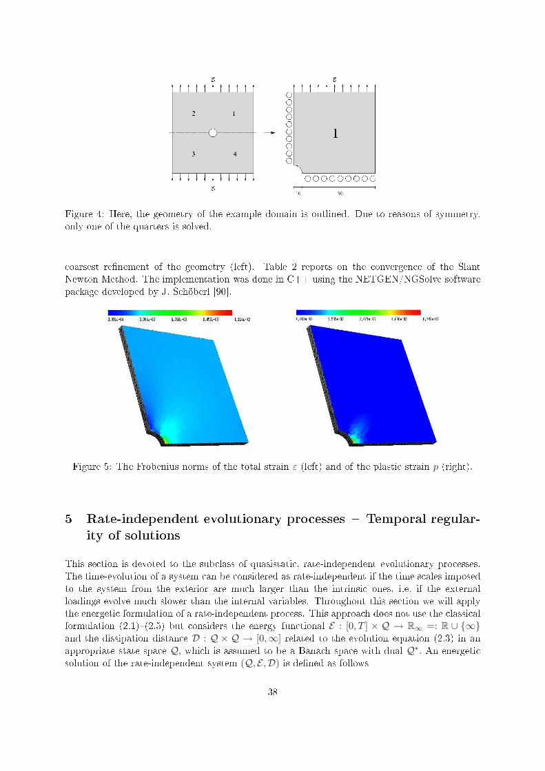
Figure 4: Here, the geometry of the example domain is outlined. Due to reasons of symmetry,only one of the quarters is solved. oarsest renement of the geometry (left). Table 2 reports on the onvergen e of the SlantNewton Method. The implementation was done in C++ using the NETGEN/NGSolve softwarepa kage developed by J. S höberl [90.

Figure 5: The Frobenius norms of the total strain ε (left) and of the plasti strain p (right).5 Rate-independent evolutionary pro esses Temporal regular-ity of solutionsThis se tion is devoted to the sub lass of quasistati , rate-independent evolutionary pro esses.The time-evolution of a system an be onsidered as rate-independent if the time s ales imposedto the system from the exterior are mu h larger than the intrinsi ones, i.e. if the externalloadings evolve mu h slower than the internal variables. Throughout this se tion we will applythe energeti formulation of a rate-independent pro ess. This approa h does not use the lassi alformulation (2.1)(2.5) but onsiders the energy fun tional E : [0, T ] × Q → R∞ =: R ∪ ∞and the dissipation distan e D : Q × Q → [0,∞] related to the evolution equation (2.3) in anappropriate state spa e Q, whi h is assumed to be a Bana h spa e with dual Q∗. An energeti solution of the rate-independent system (Q, E ,D) is dened as follows38

DOF: 717 5736 45888 367104j=1: 1.000e+00 1.000e+00 1.000e+00 1.000e+00j=2: 1.013e-01 1.254e-01 1.367e-01 1.419e-01j=3: 7.024e-03 6.919e-03 7.159e-03 6.993e-03j=4: 1.076e-04 9.359e-05 1.263e-04 1.176e-04j=5: 2.451e-08 6.768e-07 1.744e-06 1.849e-06j=6: 7.149e-15 6.887e-12 4.874e-09 1.001e-08j=7: 4.298e-13 2.368e-14Table 2: This table outlines the onvergen e of the Slant Newton Method in 3D. We observesuper-linear onvergen e and (almost) a onstant number of iterations at ea h renement.Denition 5.1. The pro ess q=(u, z) : [0, T ] → Q is an energeti solution of the rate-independentsystem (Q, E ,D), if t 7→ ∂tE(t, q(t)) ∈ L1((0, T )), if for all t ∈ [0, T ] we have E(t, q(t)) < ∞ andif the global stability inequality (S) and the global energy balan e (E) are satised:Stability : for all q ∈ Q : E(t, q(t)) ≤ E(t, q) + D(q(t), q), (S)Energy balan e : E(t, q(t)) + DissD(q, [0, t]) = E(0, q(0)) +

∫ t

0∂ξE(ξ, q(ξ)) dξ (E)with DissD(q, [0, t]) := sup

∑Nj=1 D(q(ξj−1), q(ξj)), where the supremum is taken over all parti-tions of [0, t].In Se tion 5.1.1 we will larify the relations between the lassi al and the energeti formulation.Sin e the onditions (S) & (E) do not require that q exists, an energeti solution may in generalhave jumps with respe t to time. In parti ular, (S) provides the uniform boundedness of E(t, q(t))and hen e (E) yields that q : [0, T ] → Q is only of bounded variation in time with respe t tothe dissipation distan e providing an L1-norm in spa e. This means that in general the timederivative q is only given as a Radon-measure. Therefore, Se tion 5.2 pays spe ial attention tothe temporal regularity of energeti solutions. It is investigated how their temporal regularity an be improved due to additional onvexity assumptions on the energy E . In Se tion 5.2.1it is explained that stri t onvexity of E on Q yields ontinuity of the solutions with respe tto time. Se tion 5.2.2 deals with the Hölder- and Lips hitz- ontinuity of energeti solutions,whi h an be obtained by laiming a kind of uniform onvexity on E . In Se tion 5.3 the theoryintrodu ed in Se tion 5.2 is applied to evolutionary pro esses modeling plasti ity, damage orphase transformations in shape memory alloys and we give examples on stored elasti energydensities that lead to su h improved temporal regularity.5.1 The energeti formulation of rate-independent pro essesThe outline of this se tion is to larify the energeti formulation of rate-indepedent pro esses.Thereto Se tion 5.1.1 indi ates the relation of energeti solutions to the on ept of solution usedin the Se tions 2, 3. Moreover Se tion 5.1.2 gives a short introdu tion to the existen e theoryof energeti solutions. At this point we want to start our dis ussion with the mathemati al hara terization of rate-independen e.The energeti formulation of a rate-independent pro ess is solely based on an energy fun tional

E : [s, T ] × Q → R∞, whi h depends on time t and the state q, and a dissipation potential39

R : Q → [0,∞] depending on the velo ity q. It is assumed that the potential R is onvex andpositively 1-homogeneous, i.e. R(0) = 0 and R(λv) = λR(v) for all λ> 0 and all v ∈Q. Due tothese two properties R satises a triangle inequality, i.e. for all q1, q2, q3∈Q it holdsR(q1−q2) = 2R

(12 (q1−q3) + 1

2(q3−q2))≤ 2

(12R(q1−q3) + 1

2R(q3−q2))

= R(q1−q3) + R(q3−q2) .Hen e the dissipation potential generates a dissipation distan eD(q, q) = R(q − q) , (5.1)whi h is an extended pseudo-distan e on the state spa e Q. This means that D satises theaxioms of a metri (positivity, triangle inequality), ex ept symmetry and it may attain the value

∞, as we will see in the examples of Se tion 5.3.Rate-independen e of a pro ess (Q, E ,R) with the initial ondition q(s) = q0 ∈ Q, the givenexternal loadings b ∈ C1([s, T ],Q∗) and a solution q : [s, T ] → Q an be dened using aninput-output operatorH[s,T ] : Q× C1([s, T ],Q∗) → L∞([s, T ],Q) ∩BVD([s, T ],Q), (q0, b) 7→ q , (5.2)where BVD([s, T ],Q) := q : [s, T ] →Q|DissD(q, [s, T ])<∞. Thus, the input-output operatormaps the given data (q0, b) onto a solution of the problem. Therewith the rate-independen e ofthe system (Q, E ,R) an be hara terized as followsDenition 5.2. An evolutionary pro ess (Q, E ,R), whi h an be expressed by (5.2), is alledrate-independent if for all s⋆ < T⋆ and all α ∈ C1([s⋆, T⋆]) with α > 0 and α(s⋆) = s, α(T⋆) = Tthe following holds:

H[s⋆,T⋆](q0, b α) = H[s,T ](q0, b) α . (5.3)We verify now that the positive 1-homogeneity of R implies (5.3). We prove this impli ationfor input-output operators H[s,t] :Q×C1([s, t],Q∗)→W 1,1([s, t],Q). Thereby, Q is in general aLebesgue or Sobolev spa e dened with respe t to a domain Ω ⊂ Rd. By molli ation, see also [7,one an therefore show that for any q∈BVD([0, T ],Q) there is a sequen e (qn)n∈N⊂C∞([0, T ],Q)satisfying qn→q in L1([0, T ]×Ω), DissD(qn, [0, t])<C and DissD(qn, [0, t])→DissD(q, [0, t]) for all

t∈ [0, T ]. Thus, the above mentioned impli ation also holds true for the input-output operatorsfrom (5.2).Proposition 5.3. Let H[s,T ] : Q × C1([s, T ],Q∗) → W 1,1([s, t],Q), (q0, b) 7→ q, be the input-output-operator for the rate-independent system (Q, Eb,R), where Eb depends ontinuously on theexternal loading b and where R is onvex and positively 1-homogeneous. Then (5.3) holds true.Proof. Let s⋆ < T⋆ and α ∈ C1([s⋆, T⋆]) with α > 0 and α(s⋆) = s, α(T⋆) = T. In parti ularit holds s⋆ = α−1(s), T⋆ = α−1(T ) and (α−1)′ > 0. Assume that q : [s, T ] → Q is an energeti solution of (Q, Eb,R, ) satisfying q(s) = q0. Hen e (S)&(E) are satised for all t ∈ [s, T ]. Now thetime interval is res aled, i.e. t = α(t⋆) for all t ∈ [s, T ]. Then (S) implies that Ebα(t⋆, q α(t⋆)) ≤Ebα(t⋆, q)+D(qα(t⋆), q) for all q ∈ Q, i.e. (S) holds true for all t⋆ ∈ [s⋆, T⋆] for qα : [s⋆, T⋆] → Qand the system (Q, Ebα,R).For a fun tion q ∈ W 1,1([s, T ],Q) it holds that DissD(q, [s, t]) =

∫ ts R(q(ξ)) dξ, whi h an beveried by applying the positive 1-homogeneity of R and the mean value theorem of dieren-tiability to the denition of DissD(q, [s, t]). Then, for s = α(s⋆) and t = α(t⋆) the appli a-tion of the hain rule on q(α(t⋆)) together with the positive 1-homogeneity of R imply that40

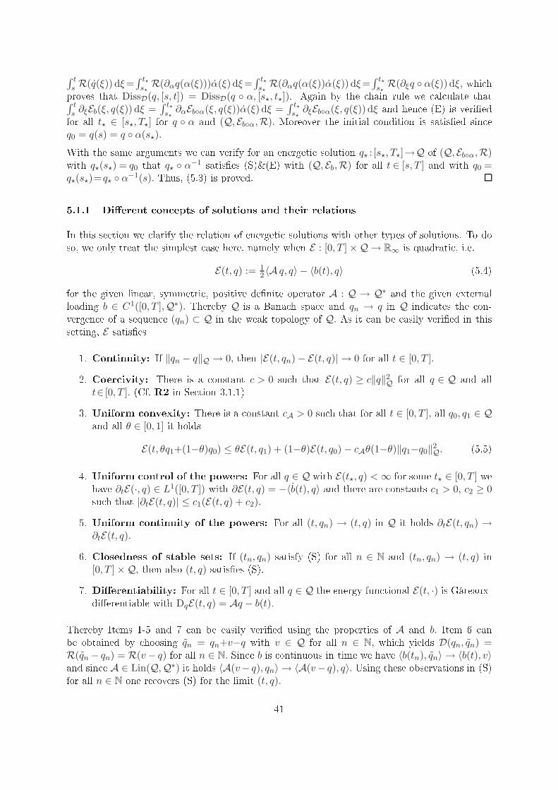
∫ ts R(q(ξ)) dξ=

∫ t⋆s⋆

R(∂αq(α(ξ)))α(ξ) dξ=∫ t⋆s⋆

R(∂αq(α(ξ))α(ξ)) dξ=∫ t⋆s⋆

R(∂ξq α(ξ)) dξ, whi hproves that DissD(q, [s, t]) = DissD(q α, [s⋆, t⋆]). Again by the hain rule we al ulate that∫ ts ∂ξEb(ξ, q(ξ)) dξ =

∫ t⋆s⋆∂αEbα(ξ, q(ξ))α(ξ) dξ =

∫ t⋆s⋆∂ξEbα(ξ, q(ξ)) dξ and hen e (E) is veriedfor all t⋆ ∈ [s⋆, T⋆] for q α and (Q, Ebα,R). Moreover the initial ondition is satised sin e

q0 = q(s) = q α(s⋆).With the same arguments we an verify for an energeti solution q⋆ : [s⋆, T⋆]→Q of (Q, Ebα,R)with q⋆(s⋆) = q0 that q⋆ α−1 satises (S)&(E) with (Q, Eb,R) for all t ∈ [s, T ] and with q0 =q⋆(s⋆)=q⋆ α−1(s). Thus, (5.3) is proved.5.1.1 Dierent on epts of solutions and their relationsIn this se tion we larify the relation of energeti solutions with other types of solutions. To doso, we only treat the simplest ase here, namely when E : [0, T ] ×Q → R∞ is quadrati , i.e.

E(t, q) := 12 〈A q, q〉 − 〈b(t), q〉 (5.4)for the given linear, symmetri , positive denite operator A : Q → Q∗ and the given externalloading b ∈ C1([0, T ],Q∗). Thereby Q is a Bana h spa e and qn → q in Q indi ates the on-vergen e of a sequen e (qn) ⊂ Q in the weak topology of Q. As it an be easily veried in thissetting, E satises1. Continuity: If ‖qn − q‖Q → 0, then |E(t, qn) − E(t, q)| → 0 for all t ∈ [0, T ].2. Coer ivity: There is a onstant c > 0 su h that E(t, q) ≥ c‖q‖2

Q for all q ∈ Q and allt∈ [0, T ]. (Cf. R2 in Se tion 3.1.1)3. Uniform onvexity: There is a onstant cA > 0 su h that for all t ∈ [0, T ], all q0, q1 ∈ Qand all θ ∈ [0, 1] it holds

E(t, θq1+(1−θ)q0) ≤ θE(t, q1) + (1−θ)E(t, q0) − cAθ(1−θ)‖q1−q0‖2Q. (5.5)4. Uniform ontrol of the powers: For all q ∈ Q with E(t⋆, q) <∞ for some t⋆ ∈ [0, T ] wehave ∂tE(·, q) ∈ L1([0, T ]) with ∂E(t, q) = −〈b(t), q〉 and there are onstants c1 > 0, c2 ≥ 0su h that |∂tE(t, q)| ≤ c1(E(t, q) + c2).5. Uniform ontinuity of the powers: For all (t, qn) → (t, q) in Q it holds ∂tE(t, qn) →

∂tE(t, q).6. Closedness of stable sets: If (tn, qn) satisfy (S) for all n ∈ N and (tn, qn) → (t, q) in[0, T ] ×Q, then also (t, q) satises (S).7. Dierentiability: For all t ∈ [0, T ] and all q ∈ Q the energy fun tional E(t, ·) is Gâteaux-dierentiable with DqE(t, q) = Aq − b(t).Thereby Items 1-5 and 7 an be easily veried using the properties of A and b. Item 6 anbe obtained by hoosing qn = qn+v−q with v ∈ Q for all n ∈ N, whi h yields D(qn, qn) =

R(qn − qn) = R(v− q) for all n ∈ N. Sin e b is ontinuous in time we have 〈b(tn), qn〉 → 〈b(t), v〉and sin e A ∈ Lin(Q,Q∗) it holds 〈A(v− q), qn〉 → 〈A(v− q), q〉. Using these observations in (S)for all n ∈ N one re overs (S) for the limit (t, q).41

In Se tion 5.1.2 it is explained that the properties 16 together with the properties of the ex-tended pseudo-distan e D : Q×Q → R∞ allow to prove the existen e of an energeti solution.Furthermore in Se tion 5.2.2 it is dis ussed that property 3 yields Lips hitz- ontinuity of theenergeti solution q : [0, T ] → Q with respe t to time, i.e. there is a onstant CL > 0 su h that‖q(s)−q(t)‖Q ≤ CL|s−t|. Hen e q ∈W 1,∞([0, T ],Q), whi h means that q exists a.e. in [0, T ].Sin e the dissipation potential R : Q → [0,∞] is onvex and positively 1-homogeneous but notne essarily dierentiable we introdu e its subdierential

∂vR(v) := q∗ ∈ Q∗ |R(w) ≥ R(v) + 〈q∗, w−v〉 for all w ∈ Q . (5.6)Due to the validity of 17 and (5.6) we may onsider the subdierential formulation (SDF) andthe formulation as a variational inequality (VI), whi h dire tly use q, as alternative formulationsto the energeti one. The subdierential formulation of the evolutionary pro ess reads as followsDenition 5.4 (Subdierential formulation). For a given initial ondition q0 ∈ Q nd q :[0, T ] → Q su h that for a.e. t ∈ [0, T ] it holds

0 ∈ ∂R(q(t)) + DqE(t, q(t)) ⊂ Q∗ and q(0) = q0 ∈ Q . (SDF)Moreover (SDF) is equivalent to −DqE(t, q) ∈ ∂R(q) and due to the denition of the subdier-ential we may equivalently formulate the rate-independent pro ess as a variational inequalityDenition 5.5 (Variational inequality). For a given inital ondition q0 ∈ Q nd q : [0, T ] → Qsu h that for a.e. t ∈ [0, T ] and for all v ∈ Q it holds〈DqE(t, q), v − q〉 + R(v) −R(q) ≥ 0 and q(0) = q0 ∈ Q . (VI)Between the three dierent formulations (S) & (E), (SDF) and (VI) the following relation holdsLemma 5.6. If E : Q → R∞ satises the properties 17, if D : Q ×Q → [0,∞] is an extendedpseudo-distan e and lower semi ontinuous on the Bana h spa e Q and if q0 satises (S) at t = 0,every energeti solution of the rate-independent system (Q, E ,D) also is a solution in the senseof (SDF) as well as (VI) and vi e versa, i.e. (S)& (E) ⇔ (SDF) ⇔ (VI).Proof. Let q : [0, T ] → Q solve (S) & (E). By Theorem 5.13 we have q ∈ W 1,∞([0, T ],Q), sothat DissD(q, [0, t]) =

∫ t0 R(q(ξ)) dξ for all t ∈ [0, T ]. Hen e (E) reads E(t, q(t))+

∫ t0 R(q(ξ)) dξ =

E(0, q(0))+∫ t0 ∂tE(ξ, q(ξ)) dξ. Applying d

dt leads to ddtE(t, q(t))+R(q(t)) = ∂tE(t, q(t)) for almostall t ∈ [0, T ]. Using the hain rule on d

dtE(t, q(t)) yields〈DqE(t, q(t)), q(t)〉 + R(q(t)) = 0 . (Eloc)Furthermore, inserting q(t) + hv for v ∈ Q in (S) together with Item 7 results in

〈DqE(t, q(t)), v〉 + R(v) ≥ 0 for all v ∈ Q (Sloc)and subtra ting (Eloc) from (Sloc) nally yields (VI), whi h is equivalent to (SDF).Assume now that q solves (VI) and (SDF) for a.e. t ∈ [0, T ]. Multiply (VI) by h > 0 and putv = q

h . For h → 0 one obtains (Sloc). Due to the onvexity and the Gâteaux-dierentiablilityof E(t, ·) for all q ∈ Q we nd from (Sloc) with v = q − q(t) that 0 ≤ 〈DqE(t, q(t)), q − q(t)〉 +R(q − q(t)) ≤ E(t, q) − E(t, q(t)) + R(q − q(t)) for a.e. t ∈ [0, T ]. But sin e q : [0, T ] → Q is42

Lips hitz- ontinuous in time and sin e E(·, q) is ontinuous for all q ∈ Q we observe that (S)holds for all t ∈ [0, T ]. Now (E) has to be proven. Choosing thereto v = q(t) in (Sloc) gives〈DqE(t, q(t)), q(t)〉 + R(q(t)) ≥ 0 and v = 0 in (VI) yields 〈DqE(t, q(t)),−q(t)〉 − R(q(t)) ≥ 0,whi h proves (Eloc). By integrating (Eloc) over [0, t] we verify that (E) holds for all t ∈ [0, T ].The equivalen e established in Lemma 5.6 is in general only true for energies satisfying theuniform onvexity inequality in property 3. For onvex energies it an be veried if energeti solutions are supplied with su ient temporal regularity. In the ase of non onvex energies, orenergies whi h are onvex but not jointly onvex in q = (u, z), energeti solutions are of boundedvariation with respe t to time. Hen e they may have jumps in time and the time-derivative isonly a Radon-measure. Relations between the three dierent formulations with q as a Radon-measure are dis ussed in [70. Furthermore it omments on their relations in the ase of doublynonlinear problems, whi h were introdu ed in [27 and where E is only subdierentiable but notGâteaux-dierentiable.In many appli ations the dissipation potential only depends on the internal variable z, not onthe full state q = (u, z), i.e. R(q) = R(z), so that ∂R(q) = ∂uR(z) × ∂zR(z) = 0 × ∂R(z).This is also the ase in the setting of plasti ity studied in Se tions 2, 3. Using the dualitytheory of fun tionals one an establish a relation between the ow rule given by (2.3) and(2.9) and the dissipation potential R : Z → [0,∞] under the assumption that Z is a reexiveBana h spa e. In view of the denition of the subdierential ∂R(z) = z∗ ∈ Z∗ |R(z)−R(z) ≥〈z∗, z−z〉 for all z ∈ Z the dire t al ulation of the Legendre-Fen hel transform of the positively1-homogeneous dissipation potential R : Z → [0,∞] yields that its dual fun tional is given as theindi ator fun tion of ∂R(0), i.e. R∗(z∗) = supz∈Z

(〈z∗, z〉 − R(z)

)= I∂R(0)(z

∗) for all z∗ ∈ Z∗,where I∂R(0)(z∗) = 0 if z ∈ ∂R(0) and I∂R(0)(z

∗) = ∞ otherwise.Sin e R : Z → [0,∞] is assumed to be onvex and lower semi ontinuous on the reexive Bana hspa e Z the theorem of Fen hel-Moreau implies that R = (R∗)∗, see [51. Assume now thatthe dissipation potential is an integral fun tional, i.e. for all z ∈ Z it is R(z) =∫ΩR(z(x)) dx,where R is a positively 1-homogeneous, onvex density and Ω ⊂ R

d is a d-dimensional domain.Then [51, p. 296, Th. 1 states that R∗(·) =( ∫

ΩR(·) dx)∗

=∫ΩR

∗(·) dx, i.e. for the densityR : V → [0,∞], where V ∈ R,Rd,Rd×d, holds the analogous relation to its Legendre-Fen heltransformed: R(z) = R∗∗(z) for all z ∈ V. Thus, between the subdierential formulation (SDF)of Denition 5.4 and the ow rule given by (2.3) and (2.9) we have established the relationz ∈ g(−∇zψ(e, z)) = ∂R∗(−∇zψ(e, z)), where R∗ is the Legendre-Fen hel transformed of thedensity R of the positively 1-homogeneous dissipation potential R.Throughout this hapter we will in general onsider dissipation potentials R : Z → [0,∞] of theform

R(z) =

∫

ΩR(z) dx with R : V → [0,∞], R(z) =

|z| if z ∈ A ⊂ V ,∞ otherwise , (5.7)where 0 < 0 ≤ ∈ L∞(Ω).Example 5.7. For KvM=τ ∈ R

d×dsym,dev | |τ | ≤ c0 from Example 3.5 it is RvM (εp) = c0|εp| forall εp ∈ R

d×dsym,dev.

43

5.1.2 Existen e of energeti solutionsThe quasistati evolution of me hani al pro esses in solids su h as elasto-plasti deformations,damage, ra k propagation or onta t angle hystheresis of droplets have been analyzed in various ontributions, amongst these e.g. [28, 63, 40, 29, 16, 30. All these pro esses an be des ribed interms of an energy fun tional E and a dissipation distan e D, so that the energeti formulationfrom Denition 5.1 applies. Within the works [65, 71, 36, 69 an abstra t existen e theoryfor energeti solutions of rate-independent pro esses has been developed. It is based on theassumption that D : Z × Z → [0,∞] satisesQuasi-distan e: ∀ z1, z2, z3 ∈ Z : D(z1, z2) = 0 ⇔ z1 = z2 andD(z1, z3) ≤ D(z1, z2) + D(z2, z3);

(D1)Lower semi- ontinuity: D : Z × Z → [0,∞] is weakly seq. lower semi- ontinuous. (D2)and it uses the following assumptions on the energy E : [0, T ] ×Q → R∞Compa tness of energy sublevels: ∀ t∈[0, T ] ∀E∈R :LE(t) := q ∈ Q | E(t, q) ≤ E is weakly seq. ompa t. (E1)Uniform ontrol of the power: ∃ c0∈R ∃ c1>0 ∀ (tq, q)∈[0, T ]×Q with E(tq, q) <∞ :

E(·, q) ∈ C1([0, T ]) and |∂tE(t, q)| ≤ c1(c0+E(t, q)) for all t∈[0, T ].(E2)These properties ensure the following existen e result for energeti solutions of rate-independentpro esses.Theorem 5.8 ([69). Let (Q, E ,D) satisfy onditions (E1), (E2) and (D1), (D2). Moreover, letthe following ompatibility onditions hold: For every sequen e (tk, qk)k∈N with (tk, qk) (t, q)in [0, T ] ×Q and (tk, qk) satisfying (S) for all k ∈ N we have

∂tE(t, qk) → ∂tE(t, q) , (C1)(t, q) satises (S) . (C2)Then, for ea h initial ondition (t = 0, q0) satisfying (S) there exists an energeti solution q :

[0, T ] → Q for (Q, E ,D) with q(0) = q0.The proof of Theorem 5.8 is based on a time-dis retization, where onditions (E1), (D2) ensurethe existen e of a minimizer for the time-in remental minimization problem at ea h time-step.Thereto the dire t method of the al ulus of variations is applied. In parti ular onditions (E1)and (D2) an be veried if E and D are onvex and oer ive. Hen e, for a given partitionΠ := 0 = t0 < t1 < . . . < tM = T, for every k = 1, . . . ,M one has tond qk ∈ argminE(tk, q) + D(zk−1, z) | q = (u, z) ∈ Q . (IP)One then denes a pie ewise onstant interpolant qΠ with qΠ(t) := qk−1 for t ∈ [tk−1, tk) andqΠ(T ) = qM . Choosing a sequen e (Πm)m∈N of partitions, where the neness of Πm tends to 0 asm→ ∞, it is possible to apply a version of Helly's sele tion prin iple to the sequen e (qΠm)m∈N,see thereto [65. Using (E2) and the ompatibility onditions (C1), (C2) it an be shown thatthe limit fun tion fullls the properties (S) and (E) of an energeti solution. See e.g. [69 for adetailed proof. 44

In various works this abstra t theory has been applied to prove the existen e of energeti solutionsto rate-independent pro esses in the eld of plasti ity, damage, delamination, ra k-propagation,hystheresis or shape memory alloys, amongst these [66, 68, 106, 87, 60, 70, 73, 72. The way toverify the abstra t onditions depends on the properties of the pro ess under onsideration. Inparti ular, unidire tional pro esses su h as damage or delamination pro esses require additionalte hiques to obtain ompatibility ondition (C2). In su h a setting the dissipation distan e takesthe form (5.7) with A 6= V , where the value ∞ models the unidire tionality, i.e. it prohibitshealing. This leads to the fa t that the dissipation distan e is neither ontinuous nor weakly ontinuous on Z, so that (C2) annot be dire tly obtained from the stability of the approximatingsequen e (tk, qk) → (t, q) in [0, T ] ×Q. Su h unidire tional pro esses and alternative te hniquesto prove (C2) are studied in [68, 106, 87.Finally it is worth mentioning that the quadrati energy dened in (5.4), whi h satises Items17 ts into the abstra t setting of (E1), (E2) and Theorem 5.8.5.2 The temporal regularity of energeti solutionsThe two properties (S)& (E) provide a very weak result on the temporal regularity of an energeti solution only. (S) implies that E(t, q(t)) is uniformly bounded for all t ∈ [0, T ] and under theassumption of oer ivity we nd q ∈ L∞([0, T ],Q). Furthermore one obtains from (E) thatDissD(z, [0, T ]) is nite and hen e z ∈ BV ([0, T ], L1(Ω)). Thus neither the omponent u norz of an energeti solution has to be ontinuous not to mention ontinuously dierentiable intime. In other words, it annot be ex luded that an energeti solution has jumps with respe tto time. The aim of this se tion is to dis uss settings whi h lead to a better temporal regularityof an energeti solution. In parti ular we want to obtain ontinuity in time, so that jumps areforbidden.5.2.1 Continuity with respe t to timeIn this se tion we dis uss the temporal ontinuity of energeti solutions, whi h an be obtainedin settings that guarantee unique minimizers of the fun tional Jz∗ : Q → R∞, Jz∗(q) = E(t, q)+D(z∗, z) for any z∗ ∈ Z. In the following the results are sket hed. The details are developed in[106, Th. 4.2, 4.3.The uniqueness of the minimizer, whi h is guaranteed by the stri t onvexity of Jz−(t), enablesto state the following jump relationsLemma 5.9 (Jump relations). Assume that (Q, E ,D) satises (E1)(C2). Moreover,

∀ t ∈ [0, T ] ∀ q = (u, z) ∈ S(t) : u = Argminu∈U

E(t, u, z). (5.8)Then, for all t ∈ [0, T ] the weak limits q−(t) = w-limτ→t− q(τ) and q+(t) = w-limτ→t+ q(τ)(where q−(0) := q(0) and q+(T ) = q(T )) exist and satisfyE(t, q−(t)) = E(t, q(t)) + D(q−(t), q(t)),

E(t, q(t)) = E(t, q+(t)) + D(q(t), q+(t)),

D(q−(t), q+(t)) = D(q−(t), q(t))+D(q(t), q+(t)).

(5.9)45

The existen e of the limits z−(t) = w-limτ→t− z(τ) and z+(t) = w-limτ→t+ z(τ) is due toDissD(z, [0, T ]) < ∞ for an energeti solution, see [65. From (E1) one nds u(t±k ) v± fort±k → t and (C2) yields that (t, v±, z±) satisfy (S). Due to assumption (5.8) the limits v± areuniquely determined and thus they are the desired left and right limits to u±(th) in the weaksense. To verify the jump relations (5.9) the energy balan e for the energeti solution q(t) is used

E(s, q(s)) + DissD(z, [r, s]) = E(r, z(r)) +

∫ s

r∂τE(τ, q(τ)) dτ for all 0 ≤ r < s ≤ T .The rst and the se ond identity in (5.9) are based on the fa t that both q−(t) and q+(t) as wellas q(t) satisfy (S). Hen e they an be obtained by onsidering s = t together with r → t− and

r = t together with s→ t+. The third identity is due to (D1) and the rst two identities.The next theorem provides the temporal ontinuity of the energeti solution q = (u, z) : [0, T ] →Q = U×Z in the ase that the energy E(t, ·) is stri tly onvex on Q. This requirement is satisedfor an energy, whi h is dened via a stored elasti energy density W : R

m → R∞ being stri tly onvex on Rm, i.e. for a bounded domain Ω ⊂ R

d it is E(t, u, z) :=∫ΩW

(F (u+uD(t), z)

)dx−

〈b(t), u+uD(t)〉. Thereby F (u, z) stands for all o uring omponents of the pair (u, z) andall o uring derivatives, e.g. F (u, z) = (e(u), z) for kinemati hardening, whereas F (u, z) =(e(u), z,∇z) for damage. In parti ular, F (u, z) has to be of su h a form that it indu es a normfor (u, z) on Q.Theorem 5.10. Let the stored elasti energy density W : R

m → R∞ be ontinuous and stri tly onvex on Rm. Let the the given data satisfy uD ∈ C1([0, T ],U), b ∈ C1([0, T ],U∗). Then for all

t ∈ [0, T ], z∗ ∈ Z the fun tional Jz∗(t, q) =∫ΩW (F (u+uD(t), z)) dx−〈b(t), u+uD(t)〉+D(z∗, z)is stri tly onvex in q. Assume that q = (u, z) : [0, T ] → Q is an energeti solution to (Q, E ,D).Then q is (norm-) ontinuous with respe t to time, i.e. q ∈ C0([0, T ],Q).The stri t onvexity allows us to show that energeti solutions q = (u, z) : [0, T ] → Q have weakleft and right limits q−(t) and q+(t) for all t ∈ [0, T ]. Exploiting the jump relations one obtainsthat q−(t), q(t) and q+(t) all provide the same value Jz−(t)(t, q−(t)), whi h has to be the globalminimum by stability of q−(t). Sin e the stri t onvexity of Jz−(t) guarantees a unique minimizer,all three states must oin ide and weak ontinuity follows. Strong ontinuity is dedu ed from aresult of Visintin [109, 2 & Th. 8, whi h onverts weak onvergen e and energy onvergen einto strong onvergen e by exploiting the stri t onvexity on e again.5.2.2 Hölder- and Lips hitz- ontinuity in timeThe temporal Hölder- or Lips hitz- ontinuity is based on the uniform onvexity of the fun tional

Jz∗(t, q) = E(t, q) + D(z∗, z) on a subset of a suitable Bana h spa e V. As we will see in theexamples of Se tion 5.3, the Bana h spa e V may dier signi antly from the state spa e Qthat is used to prove existen e. This is due to fa t that the hoi e of V inuen es the temporalregularity obtained, so that the use of a bigger spa e may lead to a better temporal regularityresult. The uniform onvexity is dened as followsDenition 5.11. The fun tional J : V → R∞ is uniformly onvex on the onvex set M ⊂ V, ifthere exist onstants c⋆ > 0, 2 ≤ α <∞, su h that for all onvex ombinations qθ := θq1+(1−θ)q0with θ ∈ (0, 1) and q0, q1 ∈ M the following holdsJ (t, qθ) ≤ θJ (t, q1) + (1−θ)J (t, q0) − θ(1−θ)c⋆‖q1 − q0‖α

V . (5.10)46

For a better understanding of this notion of onvexity we rst investigate the denition forreal valued, s alar fun tions. A fun tion f : R → R is uniformly onvex if there are onstants2 ≤ α <∞, c⋆ > 0 su h that for all onvex ombinations qθ = (1−θ)q0 + θq1 with θ ∈ (0, 1), q0,q1 ∈ R the following holds

f(qθ) ≤ θf(q1) + (1−θ)f(q0) − θ(1−θ)c⋆|q1−q0|α . (5.11)In other words, if f : R → R is uniformly onvex, then for any two points f(q0), f(q1) of itsgraph there ts some polynomial that is quadrati in θ, between the fun tion and the hord, seeFig. 6. Hen e uniform onvexity implies stri t onvexity.PSfrag repla ements f

q0 qθ q1Figure 6: Uniformly onvex fun tion.The meaning of the exponent α an be understood from the following example.Example 5.12. First, onsider the fun tion f(q) = q2. We immediately see that f is stri tly onvex, sin e f ′′(q) = 2 > 0 for all q ∈ R and by simple al ulation we verify f(qθ) =θf(q1)+(1−θ)f(q0)−θ(1−θ)(q1−q0)2. But there are also fun tions being stri tly onvex althoughf ′′(q) = 0 for some q ∈ R. Su h a andidate is e.g. f(q) = q4 with f ′′(0) = 0. Sin e f is on-tinuously dierentiable, the uniform onvexity inequality (5.11) is equivalent to f(q1)− f(q0) ≥f ′(q0)(q1−q0) + c⋆|q1−q0|α and hen e equivalent to (f ′(q1)−f ′(q0))(q1−q0) − 2c⋆|q1−q0|α ≥ 0.Therewith we verify for c⋆ = 1/4 and α = 4 that (f ′(q1)−f ′(q0))(q1−q0) − 2c⋆|q1−q0|α =12(q1−q0)4 + 6

2(q21−q20)2 ≥ 0 and thus we on lude that (5.11) holds for f(q) = q4 with c⋆ = 1/4and α = 4.This notion of onvexity is now transfered to the ontext of energy fun tionals. The theorembelow generalizes the ideas developed in [70, 74, where Lips hitz- ontinuity with respe t to timewas derived. The generalization has two aspe ts. First it is emphasized that the onvexityproperties an be formulated with respe t to a norm ‖ ·‖V that may dier signi antly from thatunderlying the state spa e Q. In parti ular, if Q is hosen as small as possible under preservationof the oer ivity of E (see (E1)), it may be an advantage to investigate the temporal regularityof energeti solutions with respe t to the norm of a larger Bana h spa e V ⊃ Q, sin e temporalregularity may improve. Se ond, as an be seen from (5.10) the notion of uniform onvexity isnot restri ted to the exponent α = 2, so that a weaker lower bound is admissible due to α ≥ 2.Previous work [70, 74 asked α = 2 and β = 1 and enfor ed the uniform onvexity onditionon whole Q, while the theorem below only requires it on sublevels. In fa t, the formulationof the onditions on sublevels is su ient, sin e an energeti solution q : [0, T ] → Q satisesq(t) ∈ LE⋆(s) for some xed E⋆ > 0 and all s, t ∈ [0, T ]. This is due to stability (S) and thetemporal Lips hitz-estimate |E(s, q) − E(t, q)| ≤ cE |s− t| for a onstant cE > 0 and for all xedstates q ∈ Q with E(r, q) < E for some r ∈ [0, T ], whi h is a dire t onsequen e of (E2) andGronwall's inequality.Theorem 5.13 (Temporal Hölder- ontinuity). Let (Q, E ,D) be a rate-independent system, whereQ is a losed, onvex subset of a Bana h spa e X . Let LE(t) = q ∈ Q | E(t, q) ≤ E. Assume47

that there is a Bana h spa e V and that there are onstants α ≥ 2, β ≤ 1 su h that for all E∗there exist onstants C∗, c∗ > 0 so that for all t ∈ [0, T ], q0, q1 ∈ LE⋆(t) and all θ ∈ [0, 1] thefollowing holds:E(t, qθ) + D(z0, zθ) + c∗θ(1−θ)‖q1−q0‖α

V ≤ (1−θ)(E(t, q0)+D(z0, z0)

)+ θ

(E(t, q1)+D(z0, z1)

)(5.12a)|∂tE(t, q1) − ∂tE(t, q0)| ≤ C∗‖q1 − q0‖β

V , (5.12b)where (uθ, zθ) = qθ = (1−θ)q0 + θq1.Then, any energeti solution q : [0, T ] → Q of (Q, E ,D) is Hölder- ontinuous from [0, T ] to Vwith the exponent 1/(α−β), i.e. there is a onstant CH > 0 su h that‖q(s)−q(t)‖V ≤ CH|t−s|1/(α−β) for all s, t ∈ [0, T ] . (5.13)The main idea of the proof is to use uniform onvexity inequality (5.12a) to derive an improvedstability estimate, whi h ontains the additional term c∗θ(1−θ)‖q1−q0‖α

V . Using assumption(5.12b) one obtains an upper estimate for ‖q1−q0‖αV from the energy balan e. Finally the Hölderestimate (5.13) an be proved with the aid of a dierential inequality and Gronwall's lemma.The details are arried out in [106.5.3 Appli ationsIn this se tion we dis uss examples for uniformly onvex stored elasti energy densities arisingfrom various types of rate-independent pro esses, su h as plasti ity, phase transformations inshape memory alloys and damage. All these appli ations an be treated as rate-independentpro esses in terms of the energeti formulation. As the unknowns their models involve the thelinearized strain tensor e(u) = 1

2(∇u+∇uT ) in terms of the displa ement eld u : Ω → Rd and aninternal variable z whi h may be s alar-, ve tor- or tensor valued depending on the problem. Theway, how u and z are linked in the model diers and here we distinguish between energies, whi h ompose the dierent variables additively, su h as in the Example 3.5 for kinemati hardening,and energies whi h use a multipli ative omposition of the variables, su h as in the ase ofdamage, see Examples 5.165.18.5.3.1 Additive energies: Plasti ity, phase transformations in shape memory alloysIn the following we treat two appli ations with quadrati energies. We will obtain that V = Q inthese settings, that α = 2 and β = 1, so that energeti solutions are Lips hitz- ontinuous withrespe t to time. This regularity is in good a ordan e with the results proven in [70 and with lassi al existen e results for elastoplasti ity.Example 5.14. As a rst example for Theorem 5.13 we onsider the parti ular situation where

E(t, ·) is quadrati . Let Q be a reexive Bana h spa e and assume that A ∈ Lin(Q,Q∗) is alinear, bounded operator with 〈Aq, q〉 ≥ c‖q‖2Q for all q ∈ Q and for some onstant c > 0. Given

qD ∈ C1([0, T ],Q) and b ∈ C1([0, T ],Q∗) the energy E : [0, T ] ×Q → R is dened byE(t, q) = 1

2〈A(q+qD(t)), (q+qD(t))〉 − 〈b(t), q+qD(t)〉 .48

Moreover assume that the dissipation distan e D : Z × Z → [0,∞] is dened as D(z1, z2) =R(z2−z1) with R : Z → [0,∞) being positively 1-homogeneous, onvex, weakly sequentiallylower semi ontinuous and satisfying R(z) ≤ cR‖z‖Z for all z ∈ Z and for a onstant cR > 0.Then, for all qi ∈ Q, the system (Q, E ,D) satises the assumptions (5.12) with V = Q, α = 2and β = 1. Thus, from (5.13) we obtain that energeti solutions q : [0, T ] → Q are Lips hitz- ontinuous with ‖q(s) − q(t)‖Q ≤ CH |s− t| 1

2−1 .Thereby the uniform onvexity inequality (5.12a) is a dire t onsequen e of (5.5) and the on-vexity of D. Estimate (5.12b) an be vieried by straight forward al ulations.Observe that the models of elastoplasti ity with linear kinemati hardening and of elastoplasti itywith Cosserat mi ropolar ee ts from Examples 3.5 and 3.6 t into this framework. Let us nallynote that the result on the temporal Lips hitz- ontinuity due to Theorem 5.13 is in a ordan ewith known results for equations of this type, see e.g. [17, 47.Example 5.15 (The Souza-Auri hio model for thermally driven phase transformations in shapememory alloys[73). In the ontext of phase transformations in shape memoryalloys the internal variable z : Ω → Rd×dsym,dev is the mesos opi transformation strain ree tingthe phase distribution. The dissipation distan e, whi h measures the energy dissipated due tophase transformation, is assumed to take the form D(z, z) = ‖z−z‖L1(Ω) with > 0.The phase transformations are onsidered to be thermally indu ed. For a body that is small inat least one dire tion, it is reasonable to assume that the temperature ϑ ∈ C1([0, T ],H1(Ω)),with Cϑ := ‖ϑ‖C1([0,T ],H1(Ω)), is a priori given, sin e it inuen es the transformation pro ess likean applied load, see [10. Thus the energy density takes the form

W (F (u, z), ϑ) = 12

(e(u)−z

): B(ϑ) :

(e(u)−z

)+ h(z, ϑ) + σ

2 |∇z|2with the onstant σ > 0 and the elasti ity tensor B ∈ C1([ϑmin, ϑmax],R(d×d)×(d×d)) beingsymmetri and positive denite for all ϑ, i.e. there are onstants cB1 , cB2 > 0 so that cB1 |A|2 ≤ A :

B : A ≤ cB2 |A|2 for all A ∈ Rd×d. Moreover, let cBϑ := ‖B‖C1([ϑmin,ϑmax],R(d×d)×(d×d)). The fun tion

h : Rd×dsym,dev × R → R is given by

h(z, ϑ) := c1(ϑ)√δ2 + |z|2 + c2(ϑ)|z|2 + 1

δ (|z|−c3(ϑ))3+ ,where δ > 0 is onstant and ci ∈ C1([ϑmin, ϑmax]) with 0 < c1i ≤ ci(ϑ) for all ϑ ∈ [ϑmin, ϑmax]and cϑi := ‖ci‖C1([ϑmin,ϑmax]), i = 1, 2, 3. Thereby c1(ϑ) is an a tivation threshold for the initi-ation of martensiti phase transformations, c2(ϑ) measures the o uren e of an hardening phe-nomenon with respe t to the internal variable z and c3(ϑ) represents the maximum modulus oftransformation strain that an be obtained by alignment of martensiti variants. Furthermore(f)+ := max0, f. For given data b ∈ C1([0, T ],H−1(Ω,Rd)) and uD ∈ C1([0, T ],H1(Ω,Rd))the energy fun tional is dened by E(t, q) =

∫ΩW (F (u+uD(t), z), ϑ) dx−〈b(t), u+uD(t)〉. Hen ewe have

∂tE(t, q) =

∫

Ω

(∂uW (F (u+uD, z), ϑ) : e(uD)+ϑ ∂ϑW (F (u+uD, z), ϑ)

)dx− 〈b, u+uD〉 − 〈b, uD〉,

∂uW (F (u+uD, z), ϑ) : uD = (e(u+uD)−z):B(ϑ):e(uD) ,

ϑ ∂ϑW (F (u+uD, z), ϑ) = ϑ((e(u+uD)−z):∂ϑB(ϑ):(e(u+uD)−z) + ∂ϑh(ϑ, z)

).To gain a Lips hitz-estimate for ∂tE(t, ·) for the present model it is important that Theorem 5.13is formulated for energy-sublevels LE⋆(t) = q ∈ Q | E(t, q) ≤ E⋆, sin e this provides the bound49

‖ui‖H1+‖zi‖H1 ≤ CE⋆. Thus for all (u0, z0), (u1, z1) ∈ LE⋆(t) it holds∫

Ω|ϑ

(e(u1−u0)−(z1−z0)

):∂ϑB(ϑ):

(e(u1−u0)−(z1−z0)

)|dx ≤ Cϑc

B

ϑ

(‖e(u1−u0)‖L2+‖z1−z0‖L2

)2

≤ CϑcB

ϑ

( 1∑

i=0

‖e(ui)‖L2+‖zi‖L2

)(‖e(u1−u0)‖L2+‖z1−z0‖L2

)

≤ 2CE⋆CϑcB

ϑ

(‖u1−u0‖H1+‖z1−z0‖L2

).Furthermore the appli ation of the main theorem on dierentiable fun tions yields

|√δ2+|z1|2−

√δ2+|z0|2| ≤ |z1−z0|,

||z1|2−|z0|2| ≤ 2(|z1|+|z0|)|z1−z0|,|(|z1|−c3(ϑ))3+−(|z0|−c3(ϑ))3+| ≤ 2(|z1|+|z0|)2|z1−z0|,so that

∫

Ω|∂ϑh(ϑ, z1)−∂ϑh(ϑ, z0)| ≤ ‖z1−z0‖L1

(cϑ1 + 2(Ld(Ω)CE⋆)

12 cϑ2 + 6

δ cϑ3CE⋆

)≤ C⋆‖z1−z0‖L2with C⋆ := Ld(Ω)

12

(cϑ1 + 2(Ld(Ω)CE⋆)

12 cϑ2 + 6

δ cϑ3CE⋆

), where Ld(Ω) denotes the d-dimensionalLebesgue-measure of Ω. Therefore Lips hitz-estimate (5.12b) holds true with β = 1 and with

C⋆ = (C⋆ + 2CE⋆CϑcB

ϑ + cBϑcD + cl).Now it has to be veried that the density W is uniformly onvex with respe t to F (u, z). Theretowe rst al ulate that wθ:B(ϑ):wθ ≤ θw1:B(ϑ):w1+(1−θ)w0:B(ϑ):w0−θ(1−θ)cB1 |w1−w0|2 forwi=ei−zi with (ei, zi) ∈ R

d×dsym × R

d×dsym,dev, i = 0, 1, wθ = θw1 + (1−θ)w0 with θ ∈ (0, 1).Thereby a binomi formula and the positive deniteness of B(ϑ) for all ϑ were applied. Theuniform onvexity of |∇z|2 = ∇z : ∇z an be obtained similarly. We now show that h is uni-formly onvex. We immediately see that h1(z) := (δ2 + |z|2) 1

2 is onvex in z. Furthermore,sin e h3(z) := (|z| − c3(ϑ))3+ is the omposition of the monotone fun tion x3 and the onvexfun tion (·)+, we on lude that also h3(z) is onvex in z. Additionally we obtain with similar al ulations as applied for the other quadrati terms that h2(z) := |z|2 is uniformly onvex. Sin eci(ϑ) ≥ c1i > 0 for all ϑ ∈ [ϑmin, ϑmax] and i = 1, 2, 3 we have proven that h is uniformly onvexin z with h(zθ, ϑ) ≤ θh(z1, ϑ) + (1−θ)h(z0, ϑ) − θ(1−θ)c12|z1−z0|2. Summing up all terms andtaking into a ount all prefa tors yields a uniform onvexity estimate for W, whi h leads toE(t, qθ) ≤ θE(t, q1) + (1−θ)E(t, q0) − θ(1−θ)

(cB

12 ‖w1−w0‖2

L2 + σ2 ‖∇(z1−z0)‖2

L2 + c12‖z1−z0‖2L2

).Thereby we have used that the term des ribing the work of the external loadings is linear in u.Moreover we nd with Korn's inequality that ‖w1−w0‖2

L2 ≥ 12‖e(u1)−e(u0)‖2

L2 − ‖z1−z0‖2L2 ≥

12C2

K‖u1−u0‖2

H1 − ‖z1−z0‖2L2 . Under the assumption that (c12 − (cB1 /2)) > 0 we on lude that(5.12a) holds for α = 2, c∗ := min

cB1 /(4C

2K), σ/2, (c12−(cB1 /2))

and the spa eV = Q = u ∈ H1(Ω,Rd) | u = 0 on ΓD × z ∈ H1(Ω,Rd×d

sym,dev).Hen e any energeti solution q : [0, T ] → Q is temporally Lips hitz- ontinuous: q ∈ C0,1([0, T ],Q).50

5.3.2 Multipli ative energies: DamageIn the following we apply the temporal regularity results stated in Theorems 5.10 and 5.13 toenergies used in the modeling of partial, isotropi damage pro esses. Thereby, damage meansthe reation and growth of ra ks and voids on the mi ro-level of a solid material. To des ribethe inuen e of damage on the elasti behavior of the material one denes an internal variable,the damage variable z(t, x) ∈ [z⋆, 1], as the volume fra tion of undamaged material in a neigh-bourhood of material dependent size around x ∈ Ω at time t ∈ [0, T ]. Thus z(t, x)=1 meansthat the material around x is perfe tly undamaged, whereas z(t, x)=z⋆ ≥ 0 stands for maximaldamage of the neighbourhood. The ondition z⋆ > 0 models partial damage and the fa t thatz is s alar valued ree ts the isotropy of the damage pro ess, whi h means that the ra ks andvoids are presumed to have a uniform orientation distribution in the material. Furthermore itis assumed that damage is a unidire tional pro ess, so that healing is forbidden and z(t, x) ≤ 0.This ondition is preserved by the dissipation distan e, i.e. for > 0 it is

D(z0, z1) :=

∫Ω (z0 − z1) dx if z1 ≤ z0,

∞ else, (5.14)whi h punishes a de rease of damage with the value ∞. The energy in the framework of damageis given byE(t, u, z) :=

∫

ΩW (e(u+uD(t)), z) dx+

∫

Ω

κ

r|∇z|r dx−

∫

Ωl(t)(u+uD(t)) dx . (5.15)The rst term in (5.15) is the stored elasti energy, the se ond des ribes the inuen e of damagewith 1 < r <∞ and κ > 0 and the third term a ounts for the work of the external loadings.As in the previous se tions we set W (F (u, z)) = W (e(u+uD(t)), z)+ κ

r |∇z|r. In engineering, seee.g. [64, a typi al ansatz for the stored elasti energy density is the followingW (e, z) := f1(z)W1(e) +W2(e) + f2(z) and ∂zW (e, z) ≥ 0 . (5.16)In Se tion 5.2.1 we obtained that the joint stri t onvexity of W in (z, e) will ensure the temporal ontinuity of the energeti solution. But the ru ial point, whi h may spoil this regularity inthe ase of damage is, that not many stored elasti energy densities W (e, z) := f1(z)W1(e), thatsatisfy ∂zW (e, z) ≥ 0, are also jointly stri tly onvex, although both f1, W1 may be onvex. Asa negative example we present the wellknown (1−d)-model for isotropi damage, see e.g. [64:Example 5.16. For the symmetri , positive denite fourth order tensor B the stored elasti energy density

W (e, d) =(1−d)

2e:B:e =

z

2e:B:e = W (e, z)is not jointly onvex in (e, z). This an be seen from al ulating the Hessian; evaluating it in

(e, z)=(e, 1), e ∈ Rd×dsym , in the dire tion (e, z)=(− e

2 , 1) yields D2W (e, z)[(e, z), (e, z)] = ze:B:e+

2ze:B:e = −34 e:B:e < 0.To nd a positive example on stored elasti energy densities satisfying (5.16) one may use theideas of [88. 51

Example 5.17. For B as in Example 5.16 the energy density W (e, z) := e:B:e2(2−z) is jointly onvexin (e, z) and

W (e, z) :=e:B:e

2(2−z) +z2

2is stri tly onvex in (e, z). Cal ulating the Hessian yieldsD2W (e, z)[(e, z), (e, z)] =

ze:B:ze

(2−z)3 − 2ze:B:e

(2−z)2 +e:B:e

(2−z) =1

2−z (e−e):B:(e−e) ≥ 0with e := ze/(2−z) for all (e, z) ∈ Rd×dsym × [z⋆, 1]. Sin e we have D2W (e, z)[(e, z), (e, z)] = 0 forall (0, z) whenever e = 0, we nd that W is jointly, but not stri tly onvex. We on lude that

W is jointly stri tly onvex due to the term f(z) = z2

2 , sin e f ′′(z) = 1, so that f ′′(z)z2 > 0for all z 6= 0, whi h ensures that D2W (e, z)[(e, z), (e, z)]>0 for all (e, z) 6= 0 and for all (e, z)∈R

d×dsym × [z⋆, 1].Finally we dis uss an example whi h refers to Theorem 5.13 on the Hölder-and Lips hitz- ontinuity of energeti solutions. With this example we want to point out the importan e ofthe Bana h spa e V. We will see that its hoi e is not unique and that it may lead to dierent onstants α > 2. This is due to the fa t that the energy will be hosen non-quadrati in ontrastto the Examples 5.145.15. We will larify how the spa e V inuen es the magnitude of theHölder onstant and explain how to a hieve better regularity by a lever identi ation of V.Example 5.18 (The ee tive use of V). For B as above and onstants a, a, c > 0 onsider

W (e, z,∇z) :=e:B:e

2√

2−z +G(e) + a2z

2 + κ2 |∇z|2 with G(e) := c

4(a+|dev e|2)2 (5.17)with the deviator dev e := e− tr ed Id and the energy

E(t, u, z) :=

∫

ΩW (e+eD(t), z,∇z) dx −

∫

Ωb(t)(u+uD(t)) dx.We now determine V suitably. We rst treat the ase of time-dependent Diri hlet data, asinvestigated in [106. Similarly to the ideas applied in Example 5.12 we thereto dedu e thefollowing uniform onvexity inequality for W

W (eθ, zθ) ≤ (1−θ)W (e0, z0) + θW (e1, z1) − θ(1−θ)c(|E|2 + |Z|2 + |devE|4 + |∇Z|2

) (5.18)with E := e1−e0, Z := z1−z0. For q0, q1 ∈ LE⋆(t) we an verifyE(t, qθ) ≤ (1−θ)E(t, q0) + θE(t, q1) − θ(1−θ)c⋆

(‖E‖L2 + ‖Z‖L2 + ‖devE‖L4 + ‖∇Z‖L2

)α(5.19)for α = 4, c⋆ = 2−3c min(2E⋆)2−α, (2E⋆)

4−α. This estimate determines the Bana h spa eV1 := u ∈ H1(Ω,Rd) | dev e(u) ∈ L4(Ω,Rd×d) × z ∈ H1(Ω) .At this point we noti e that the right-hand side of (5.19) is in reased if we use the Lp(Ω,Rd×d)-norm for some 1 < p ≤ 4, whi h would lead to a smaller α = max2, p and hen e to a Hölderexponent loser to 1. 52

In order to nd out whether the hoi e of p = 2 is suitable, assumption (5.12b) has to beinvestigated. Thereto we al ulate∂tE(t, u, z)=

∫

Ω∂eW (e(u)+eD(t), z,∇z):eD(t) dx−

∫

Ωb(t)(u+uD(t)) dx−

∫

Ωb(t)uD(t) dx .The term DG(dev e):e = c(a+|dev e|2) 4−2

2 (dev e):e, with G dened in (5.17), plays the de isiverole in estimate (5.12b). Using Taylor expansion one an prove that∣∣DG(dev(e1)):eD(t) − DG(dev(e0)):eD(t)∣∣ ≤ C

(1+W0+W1

) p−2p |devE|,where Wi=W (ei, zi,∇zi), ei=ei+eD(t), eD(t)=e(uD(t)) and eD(t)∈C0([0, T ],W 1,∞(Ω,Rd×d)).Thus integration and Hölder's inequality with p=2 and p′=2 yield

∫

Ω

∣∣DG(dev(e1+eD(t))):eD(t) − DG(dev(e0+eD(t))):eD(t)∣∣ dx ≤ C1‖devE‖

L42≤ C2‖u1−u0‖H1with ei = e(ui) for (ui, zi) ∈ LE⋆(t). This implies β = 1 and it is suitable to introdu e the Bana hspa e

V2 := u ∈ H1(Ω,Rd) × z ∈ H1(Ω) .With this hoi e of V = V2 we have α = 2, whi h leads to the Hölder exponent 1α−1 = 1, sothat an energeti solution q : [0, T ] → Q satises q ∈ C0,1([0, T ],V2), whereas V = V1 yields

q ∈ C0, 13 ([0, T ],V1).Finally we onsider the ase of time-independent Diri hlet data uD, i.e. uD(t) = 0 for all t ∈ [0, T ].Then we have ∂tE(t, q)=−

∫Ω b(t)(u+uD) dx. Therefore we may drop ‖E‖Lp in (5.19) and hoose

V = Q. For this hoi e we nd α = 2 and the Hölder-exponent 1/(α−1) = 1, whi h means thatthe energeti solution is Lips hitz- ontinuous in time. This is in a ordan e to the regularityresult obtained [70, where only time-independent Diri hlet data were applied.A knowledgementD. K. and S. N. thank the GAMM for the possibility to organize a Young Resear hers' Minisym-posium at the GAMM Annual Meeting 2009 in Gda«sk, where this paper was initiated.P. G. is pleased to a knowledge nan ial support by the Austrian s ien e fund FWF under grantSFB F013/F1306.D. K. a knowledges the partial nan ial support by the Robert Bos h Stiftung within the FastTra k Programme.S. N. a knowledges the nan ial support by the Alexander von Humboldt Stiftung within FeodorLynen Fellowship Programme. S. N. thanks F. Murat for pointing out a mistake in the proof ofthe existen e result in [82.M. T.'s thanks go to A. Mielke and T. Roubí£ek for many fruitful dis ussions. Her resear hwas funded by the DFG within the Resear h Training Group 1128 Analysis, Numeri s andOptimization of Multiphase Problems.Bibliography[1 H.-D. Alber. Materials with Memory. Initial-Boundary Value Problems for Constitutive Equations withInternal Variables, volume 1682 of Le ture Notes in Mathemati s. Springer, Berlin, 1998.53

[2 H.-D. Alber and K. Cheªmi«ski. Quasistati problems in vis oplasti ity theory I: Models with linear hard-ening. In I. Gohberg, A.F. dos Santos, F.-O. Spe k, F.S. Teixeira, and W. Wendland, editors, Theoreti alMethods and Appli ations to Mathemati al Physi s., volume 147 of Operator Theory. Advan es and Appli- ations, pages 105129. Birkhäuser, Basel, 2004.[3 H.-D. Alber and K. Cheªmi«ski. Quasistati problems in vis oplasti ity theory. II. Models with nonlinearhardening. Math. Models Meth. Appl. S i., 17(2):189213, 2007.[4 H.-D. Alber and S. Nesenenko. Lo al and global regularity in time dependent vis oplasti ity. In B. DayaReddy, editor, IUTAM Symposium on Theoreti al, Computational and Modelling Aspe ts of Inelasti Media,volume 11 of IUTAM Bookseries, pages 363372. Springer, Netherlands, 2008.[5 H.-D. Alber and S. Nesenenko. Lo al H1-regularity and H1/3−δ-regularity up to the boundary in timedependent vis oplasti ity. Asymtoti Analysis, 63(3):151187, 2009.[6 Jo hen Alberty, Carsten Carstensen, and Darius Zarrabi. Adaptive numeri al analysis in primal elastoplas-ti ity with hardening. Comput. Methods Appl. Me h. Engrg., 171(3-4):175204, 1999.[7 L. Ambrosio, N. Fus o, and D. Pallara. Fun tions of Bounded Variation and Free Dis ontinuity Problems.Oxford University Press, 2005.[8 Gabriele Anzellotti. On the existen e of the rates of stress and displa ement for Prandtl- Reuss plasti ity.Q. Appl. Math., 41:181208, 1983.[9 H. Attou h and M. Thera. A general duality prin iple for the sum of two operators. J. Convex Anal.,3(1):124, 1996.[10 F. Auri hio. A robust integration algorithm for a nite-strain shape-memory-alloy superelasti model. Int.J. Plasti ity, 17:971990, 2001.[11 V. Barbu. Nonlinear Semigroups and Dierential Equations in Bana h Spa es. Editura A ademiei,Bu harest, 1976.[12 A. Bensoussan and J. Frehse. Asymptoti behaviour of Norton-Ho's law in plasti ity theory and H1regularity. In J.-L. Lions and C. Baio hi, editors, Boundary value problems for partial dierential equationsand appli ations, volume 29 of RMA, pages 325. Masson, Paris, 1993.[13 A. Bensoussan and J. Frehse. Asymtoti behaviour of the time dependent Norton-Ho law in plasti iytheory and H1loc regularity. Comment. Math. Univ. Carolinae, 37(2):285304, 1996.[14 Mi hael Bildhauer and Martin Fu hs. Continuity properties of the stress tensor in the 3-dimensional Ram-berg/Osgood model. J. Appl. Anal., 13(2):209233, 2007.[15 H. Blum and J. Frehse. Boundary dierentiability for the solution to Hen ky's law of elasti plasti planestress. Preprint SFB 611 435, University Bonn, 2008.[16 B. Bourdin, G. Fran fort, and J.-J. Marigo. The variational approa h to fra ture. J. Elasti ity, 91:5148,2008.[17 Haïm Brézis. Opérateurs maximaux monotones et semi-groupes de ontra tions dans les espa es de Hilbert.North-Holland Mathemati s Studies, 1973.[18 M. Bulí£ek, J. Frehse, and J. Málek. On boundary regularity for the stress in problems of linearizedelasto-plasti ity. Preprint SFB 611 443, University Bonn, 2009.[19 A. Bumb and D. Knees. Global spatial regularity for a regularized elasto-plasti model. WIAS PreprintNo. 1419, Weierstrass Institute for Applied Analysis and Sto hasti s, Berlin, 2009.[20 C. Carstensen and S. Müller. Lo al stress regularity in s alar non onvex variational problems. SIAM J.Math. Anal., 34(2):495509, 2002.[21 Carsten Carstensen. Domain de omposition for a non-smooth onvex minimization problem and its appli- ation to plasti ity. Numer. Linear Algebra Appl., 4(3):177190, 1997.[22 K. Cheªmi«ski. Global existen e of weak-type solutions for models of monotone type in the theory ofinelasti deformations. Math. Methods Appl. S i., 25:11951230, 2002.[23 K. Cheªmi«ski and P. Gwiazda. Nonhomogenious initial boundary value problems for oer ive and self- ontrolling models of monotone type. Continuum Me h. Thermodyn., 12:217234, 2000.[24 K. Cheªmi«ski and Z. Naniewi z. Coer ive limits for onstitutive equations of monotone-gradient type.Nonlin. Anal., 48:11971214, 2002.[25 Krzysztof Cheªmi«ski and Patrizio Ne. H1lo -stress and strain regularity in Cosserat plasti ity. Z. Angew.Math. Me h., 89(4):257266, 2009. 54

[26 Xiaojun Chen, Zuhair Nashed, and Liqun Qi. Smoothing methods and semismooth methods for nondier-entiable operator equations. SIAM Journal on Numeri al Analysis, 38(4):12001216, 2000.[27 P. Colli and A. Visintin. On a lass of doubly nonlinear evolution equations. Commun. in Partial DierentialEquations, 15(5):737756, 1990.[28 G. Dal Maso, A. De Simone, and M. G. Mora. Quasistati evolution problems for linearly elasti - perfe tlyplasti materials. Ar h. Ration. Me h. Anal., 180:237291, 2006.[29 G. Dal Maso, G. Fran fort, and R. Toader. Quasistati ra k growth in nonlinear elasti ity. Ar h. Ration.Me h. Anal., 176(2):165225, 2004.[30 A. De Simone, N. Grunewald, and F. Otto. A new model for onta t angle hysteresis. Netw. Heterog. Media(ele troni ), 2007.[31 A. Demyanov. Regularity of stresses in Prandtl-Reuss perfe t plasti ity. Cal . Var. Partial Dier. Equ.,34(1):2372, 2009.[32 G. Duvaut and J.L. Lions. Inequalities in Me hani s and Physi s, volume 219 of A Series of ComprehensiveStudies in Mathemati s. Springer, Berlin, 1976.[33 C. Ebmeyer. Mixed boundary value problems for nonlinear ellipti systems with p-stru ture in polyhedraldomains. Math. Na hri hten, 236:91108, 2002.[34 Ivar Ekeland and Roger Témam. Convex analysis and variational problems, volume 28 of Classi s in AppliedMathemati s. So iety for Industrial and Applied Mathemati s (SIAM), Philadelphia, PA, english edition,1999. Translated from the Fren h.[35 J.R. Fernández, W. Han, M. Sofonea, and J.M. Viaño. Variational and numeri al analysis of a fri tionless onta t problem for elasti -vis oplasti materials with internal state variables. Q. J. Me h. Appl. Math.,54(4):501522, 2001.[36 G. Fran fort and A. Mielke. Existen e results for a lass of rate-independent material models with non onvexelasti energies. J. reine angew. Math., 595:5591, 2006.[37 J. Frehse and D. Löba h. Hölder ontinuity for the displa ements in isotropi and kinemati hardening withvon Mises yield riterion. Z. Angew. Math. Me h., 88(8):617629, 2008.[38 M. Fu hs. On a lass of variational problems related to plasti ity with polynomial hardening. Appl. Anal.,60:269275, 1996.[39 M. Fu hs and G. Seregin. Variational Methods for Problems from Plasti ity Theory and for GeneralizedNewtonian Fluids, volume 1749 of Le ture Notes in Mathemati s. Springer, Berlin, 2000.[40 A. Gia omini. Ambrosio-Tortorelli approximation of quasi-stati evolution of brittle fra ture. Cal . Var.Partial Dierential Equations, 22:129172, 2005.[41 D. Gilbarg and N. S. Trudinger. Ellipti partial dierential equations of se ond order. Number 224 inGrundlehren der mathematis hen Wissens haften. Springer Verlag, 1977.[42 P. Grisvard. Ellipti Problems in Nonsmooth Domains. Pitman Publishing In , Boston, 1985.[43 P. G. Gruber and J. Valdman. Solution of one-time-step problems in elastoplasti ity by a Slant NewtonMethod. SIAM J. S i. Comput., 31(2):15581580, 2009.[44 Peter G. Gruber and Jan Valdman. Solution of elastoplasti problems based on the Moreau-Yosida Theorem.SFB Report 5, Johannes Kepler University Linz, SFB F013 "Numeri al and Symboli S ienti Computing",2006.[45 Peter G. Gruber and Jan Valdman. Implementation of an elastoplasti solver based on the Moreau-YosidaTheorem. Mathemati s and Computers in Simulation, 76(1-3):73 81, 2007.[46 Peter G. Gruber and Jan Valdman. Newton-like solver for elastoplasti problems with hardening and itslo al super-linear onvergen e. SFB Report 6, Johannes Kepler University Linz, SFB F013 "Numeri al andSymboli S ienti Computing", 2007.[47 W. Han and B. D. Reddy. Plasti ity, Mathemati al Theory and Numeri al Analysis. Springer Verlag In .,New York, 1999.[48 A. Haraux. Nonlinear Evolution Equation - Global Behavior of Solutions, volume 841 of Le ture Notes inMathemati s. Springer, Berlin, 1981.[49 M. Hintermüller, K. Ito, and K. Kunis h. The primal-dual a tive set strategy as a semismooth Newtonmethod. SIAM J. Optim., 13(3):865888 (ele troni ) (2003), 2002.55

[50 Sh. Hu and N. S. Papageorgiou. Handbook of Multivalued Analysis. Volume II: Appli ations. Mathemati sand its Appli ations. Kluwer, Dordre ht, 2000.[51 A.D. Ioe and V.M. Ti homirov. Theorie der Extremalaufgaben. VEB Deuts her Verlag der Wissens haftenBerlin, 1979.[52 I.R. Iones u and M. Sofonea. Fun tional and numeri al methods in vis oplasti ity. Oxford University Press,1993.[53 C. Johnson. Existen e theorems for plasti ity problems. J. Math. Pures Appl., IX. Sér, 55:431444, 1976.[54 C. Johnson. On plasti ity with hardening. J. Math. Anal. Appl., 62(2):325336, 1978.[55 D. Knees. Regularity results for quasilinear ellipti systems of power-law growth in nonsmooth domains:boundary, transmission and ra k problems. PhD thesis, Universität Stuttgart, 2005. http://elib.uni-stuttgart.de/opus/volltexte/2005/2191/.[56 D. Knees. Global regularity of the elasti elds of a power-law model on Lips hitz domains. Math. MethodsAppl. S i., 29:13631391, 2006.[57 D. Knees. Global stress regularity of onvex and some non onvex variational problems. Ann. Mat. PuraAppl., 187:157184, 2008.[58 D. Knees. Global spatial regularity for time dependent elasto-plasti ity and related problems. WIAS-Preprint No. 1395, Weierstrass Institute for Applied Analysis and Sto hasti s, Berlin, 2009.[59 D. Knees and P. Ne. Regularity up to the boundary for nonlinear ellipti systems arising in timein remental innitesimal elastoplasti ity. SIAM J. Math. Anal., 40(1):2143, 2008.[60 Dorothee Knees, Alexander Mielke, and Chiara Zanini. On the invis id limit of a model for ra k propaga-tion. Math. Models Meth. Appl. S i. (M3AS), 18:15291569, 2008.[61 V.G. Korneev and U. Langer. The regularity of solutions of problems from plasti -ow theory. Dier.Uravn., 20(4):597515, 1984.[62 P. Krej£í. Evolution variational inequalities and multidimensional hysteresis operators. Drábek, Pavel (ed.)et al., Nonlinear dierential equations. Pro eedings of talks given at the seminar in dierential equations,Chvalati e, Cze h Republi , June 29-July 3, 1998. Bo a Raton, FL: Chapman &amp; Hall/CRC. ChapmanHall/CRC Res. Notes Math. 404, 47-110, 1999.[63 K. L. Kuttler and M. Shillor. Quasistati evolution of damage in an elasti body. Nonlinear Analysis: RealWorld Appli ations, 7:674699, 2006.[64 J. Lemaitre and R. Desmorat. Engineering damage me hani s. Springer, 2005.[65 A. Mainik and A. Mielke. Existen e results for energeti models for rate-independent systems. Cal . Var.Partial Dier. Equ., 22:7399, 2005.[66 Andreas Mainik and Alexander Mielke. Global existen e for rate-independent gradient plasti ity at nitestrain. J. Nonlinear S ien e, 19(3):221248, 2009.[67 H. Matthies. Existen e theorems in thermo-plasti ity. J. Me ., 18:659712, 1979.[68 A. Mielke and T. Roubí£ek. Rate-independent damage pro esses in nonlinear elasti ity. M3AS Math. ModelsMethods Appl. S i., 16:177209, 2006.[69 A. Mielke, T. Roubí£ek, and U. Stefanelli. Γ-limits and relaxations for rate-independent evolutionaryproblems. Cal . Var. Partial Dier. Equ., 31:387416, 2008.[70 A. Mielke and F. Theil. On rateindependent hysteresis models. Nonl. Di. Eqns. Appl. (NoDEA), 11:151189, 2004. (A epted July 2001).[71 Alexander Mielke. Evolution in rate-independent systems (Ch. 6). In C.M. Dafermos and E. Feireisl,editors, Handbook of Dierential Equations, Evolutionary Equations, vol. 2, pages 461559. Elsevier B.V.,Amsterdam, 2005.[72 Alexander Mielke, Laetitia Paoli, and Adrien Petrov. On the existen e and approximation for a 3D model ofthermally indu ed phase transformations in shape-memory alloys. SIAM J. Math. Anal., 2009. To appear.WIAS preprint 1330.[73 Alexander Mielke and Adrien Petrov. Thermally driven phase transformation in shape-memory alloys.Gakkotosho (Adv. Math. S i. Appl.), 17:667685, 2007.[74 Alexander Mielke and Ri arda Rossi. Existen e and uniqueness results for a lass of rate-independenthysteresis problems. M3AS Math. Models Methods Appl. S i., 17:81123, 2007.56

[75 E. Miersemann. Zur Regularität der quasistatis hen elasto-viskoplastis hen Vers hiebungen und Spannun-gen. Math. Na hri hten, 96:293299, 1980.[76 J.-J. Moreau. Sur l'evolution d'un systeme elasto-vis o-plastique. C. R. A ad. S i. Paris Ser. A-B, 273:118121, 1971.[77 Jean Ja ques Moreau. Proximité et dualité dans un espa e Hilbertien. Bull. So . Math. Fran e, 93:273299,1965.[78 J.J. Moreau. Appli ation of onvex analysis to the treatment of elastoplasti systems. Appl. Methods Fun t.Anal. Probl. Me h., IUTAM/IMU-Symp. Marseille 1975, Le t. Notes Math. 503, 56-89 (1976)., 1976.[79 J. Naumann and J. Wolf. Interior dierentiability of weak solutions to the equations of stationary motionof a lass of non-Newtonian uids. J. Math. Fluid Me h., 7(2):298313, 2005.[80 P. Ne and K. Cheªmi«ski. Innitesimal elasti -plasti Cosserat mi ropolar theory. Modelling and globalexisten e in the rate independent ase. Pro . Roy. So . Edinburgh Se . A, 135:10171039, 2005.[81 S. Nesenenko. Lq-almost solvability of vis o-plasti problems of monotone type. Submitted.[82 S. Nesenenko. A note on existen e result for vis oplasti models with nonlinear hardening. Math. Me h.Solids rst published on Mar h 20, 2009 as doi:10.1177/1081286509103818.[83 D. Pas ali and S. Sburlan. Nonlinear Mappings of Monotone Type. Editura A ademiei, Bu harest, 1978.[84 W. Pompe. Existen e Theorems in the Vis oplasti ity Theory. Dissertation, Darmstadt University ofTe hnology, 2003.[85 W. Pompe. Linear fun tionals on nonlinear spa es and appli ations to problems from vis oplasti ity theory.Math. Methods Appl. S i., 31(7):775792, 2008.[86 S.I. Repin. Errors of nite element method for perfe tly elasto-plasti problems. Math. Models Meth. Appl.S i., 6(5):587604, 1996.[87 T. Roubí£ek, L. S ardia, and C. Zanini. Quasistati delamination problem. Continuum Me hani s andThermodynami s, 2009. Submitted.[88 Tomá² Roubí£ek. Rate independent pro esses in vis ous solids at small strains. Math. Meth. Appl. S i.,32(7):825 862, 2008.[89 G. Savaré. Regularity results for ellipti equations in Lips hitz domains. J. Fun t. Anal., 152:176201, 1998.[90 J. S höberl. Netgen - an advan ing front 2d/3d-mesh generator based on abstra t rules. Comput.Visual.S i,1:4152, 1997.[91 G.A. Seregin. On dierential properties of weak solutions of nonlinear ellipti systems arising in plasti itytheory. Math. USSR Sbornik, 58(2):289309, 1987.[92 G.A. Seregin. On dierential properties of extremals of variational problems arising in the theory of plas-ti ity. Dier. Equations, 26(6):756766, 1990.[93 G.A. Seregin. Dierential properties of solutions of evolutionary variational inequalities in plasti ity theory.Probl. Mat. Anal., 12:153173, 1992.[94 G.A. Seregin. On the regularity of the minimizers of some variational problems of plasti ity theory. St.Petersbg. Math. J., 4(5):9891020, 1993.[95 G.A. Seregin. Remarks on the regularity up to the boundary for solutions to variational problems inplasti ity theory. J. Math. S i., 93(5):779783, 1999.[96 P. Shi. Interior regularity of solutions to a dynami y li plasti ity model in higher dimensions. Adv. Math.S i. Appl., 9(2):817837, 1999.[97 E. Showalter. Monotone Operators in Bana h Spa es and Nonlinear Partial Dierential Equations, vol-ume 49 of Mathemati al Surveys and Monographs. AMS, Providen e, 1997.[98 J.C. Simo and J.R. Hughes. Computational Inelasti ity, volume 7 of Interdis iplinary Applied Mathemati s.Springer, Berlin, 1998.[99 J.C. Simo and R. L. Taylor. Consistent tangent operators for rate-independent elasto-plasti ity. Comp.Meth. Appl. Me h. Engrg., 48:101118, 1985.[100 E. Stein. Error- ontrolled Adaptive Finite Elements in Solid Me hani s. Wiley, Chi hester, 2003.[101 M. Steinhauer. On analysis of some nonlinear systems of partial dierential equations of ontinuum me- hani s. PhD thesis, Universität Bonn, Mathematis h-Naturwissens haftli he Fakultät, 2003.57

[102 P.-M. Suquet. Evolution problems for a lass of dissipative materials. Quart. Appl. Math., 38(4):391414,1980/81.[103 L. Tartar. Interpolation non linéaire et régularité. J. Fun t. Anal., 9:469489, 1972.[104 R. Temam. Mathemati al Problems in Plasti ity. Bordas, Paris, 1983.[105 R. Temam. A generelized Norton-Ho model and the Prandtl-Reuss law of plasti ity. Ar h. Rational Me h.Anal., 95(2):137183, 1986.[106 Marita Thomas and Alexander Mielke. Damage of nonlinearly elasti materials at small strain: existen eand regularity results. WIAS-Preprint 1397, ZAMM, 2009. Submitted.[107 H. Triebel. Interpolation Theory, Fun tion Spa es, Dierential Operators. North Holland Publishing Com-pany, Amsterdam, New York, Oxford, 1978.[108 T. Valent. Boundary Value Problems of Finite Elasti ity. Springer, Berlin, 1988.[109 A. Visintin. Strong onvergen e results related to stri t onvexity. Communi ations in Partial DierentialEquations, 9(5):439466, 1984.[110 Eberhard Zeidler. Nonlinear fun tional analysis and its appli ations. II/B: Nonlinear monotone operators.New York et .: Springer-Verlag. xv, 733 p. DM 264.00 , 1990.

58