1

15.Math-Review

Wednesday Wednesday 8/16/008/16/00

15.Math-Review 2

We can use the derivatives of a function to obtain information about the maximum and minimum values the function attains.

We saw this for: functions of one variable unconstrained variables constrained variables. Here we have to be careful with the

extreme points of the domain.

We try to locate the local minima/maxima and select the global optimum from them.

Optimization

15.Math-Review 3

Unconstrained optimization

Given f(x), find f ’(x) and f ”(x). Solve for x such that f ’(x) = 0. Substitute the solution(s) into f ”(x).

If f ”(x) 0, x is a local minimum. If f ”(x) 0, x is a local maximum. If f ”(x) = 0, x is likely a point of inflection.

Optimization

15.Math-Review 4

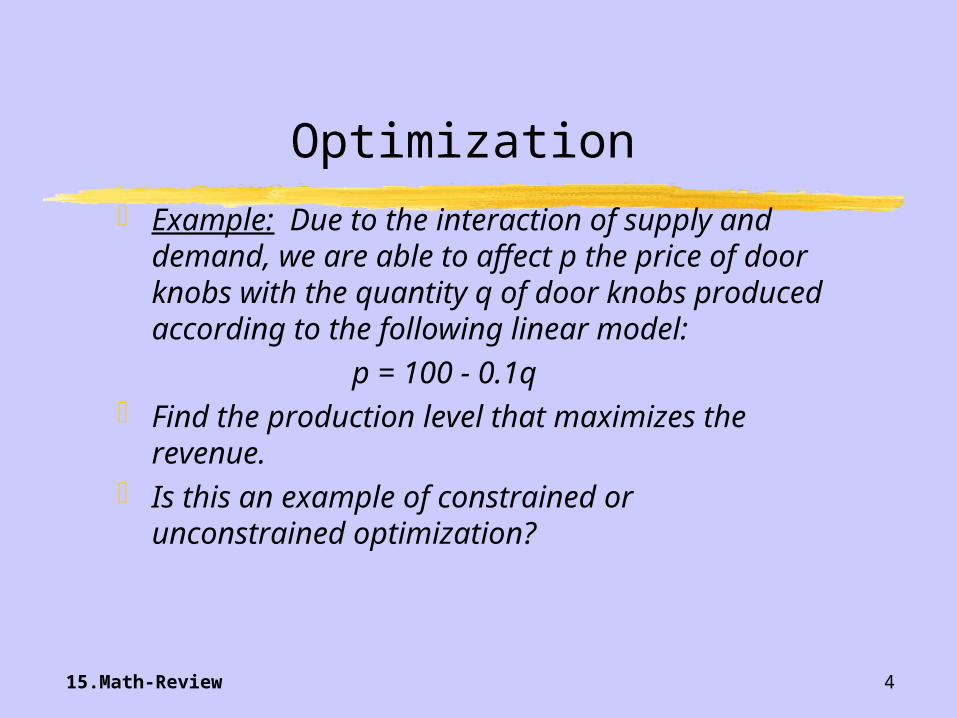
Example: Due to the interaction of supply and demand, we are able to affect p the price of door knobs with the quantity q of door knobs produced according to the following linear model:

p = 100 - 0.1q Find the production level that maximizes the

revenue. Is this an example of constrained or unconstrained

optimization?

Optimization

15.Math-Review 5

Constrained optimization Function f(x) defined for x [a, b]

Same analysis as unconstrained optimization in the interior of the domain, i.e. x (a, b).

f’(a) 0, a is a local minimum f’(a) 0, a is a local maximum f’(b) 0, b is a local maximum f’(b) 0, b is a local minimum

Optimization

15.Math-Review 6

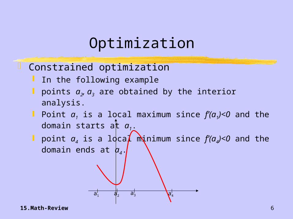
Constrained optimization In the following example points a2, a3 are obtained by the interior analysis.

Point a1 is a local maximum since f’(a1)<0 and the domain starts at a1.

point a4 is a local minimum since f’(a4)<0 and the domain ends at a4.

Optimization

a1 a2a3 a4

15.Math-Review 7

Example: In the same example of the linear model that related price with production level

p = 100 - 0.1q Consider now variable operative costs = 20q Maximize profit, with the consideration that the

production level has to be higher than 450 units due to contracts with clients.

Optimization

15.Math-Review 8

For unconstrained minimization of a multivariate function, the previous scheme generalizes easily. 1st order condition:

2nd order condition:

If these two conditions hold, x is a local minimum.

1st and 2nd order conditions

0

0

),,()(

1

)(

1

nx

xf

x

xf

nxxf

00

00

),,( )()(

)()(

1

1

111

nnn

n

xx

xf

xx

xf

xx

xf

xx

xf

nxxHf

15.Math-Review 9

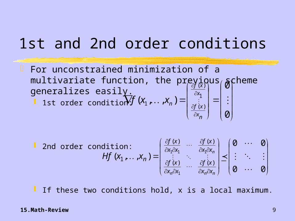
For unconstrained minimization of a multivariate function, the previous scheme generalizes easily. 1st order condition:

2nd order condition:

If these two conditions hold, x is a local maximum.

1st and 2nd order conditions

0

0

),,()(

1

)(

1

nx

xf

x

xf

nxxf

00

00

),,( )()(

)()(

1

1

111

nnn

n

xx

xf

xx

xf

xx

xf

xx

xf

nxxHf

15.Math-Review 10

Linear optimization problems consists of selecting the variables that optimize a linear objective function subject to linear constraints.

For example:

Linear Optimization

0,0

4

204

3643 s.t.

75Max

yx

x

yx

yx

yx

15.Math-Review 11

The constraints define the feasible region, in our example, we have:

Linear Optimization

0,0

4

204

1243

yx

x

yx

yx x4

4x+y20

3x+4y36

15.Math-Review 12

Note that the feasible region is bounded by lines and has vertices.

We will always find an optimal solution among the vertices of the polygon that is the feasible region.

The simplex algorithm uses a clever scheme to search for the optimal among the vertices.

The feasible region can also be unbounded (polytope) or even not exist.

Linear Optimization

15.Math-Review 13

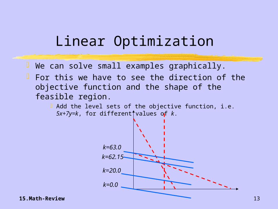
We can solve small examples graphically. For this we have to see the direction of the objective

function and the shape of the feasible region. Add the level sets of the objective function, i.e. 5x+7y=k, for

different values of k.

Linear Optimization

k=0.0

k=20.0

k=62.15

k=63.0

15.Math-Review 14

Exercise: A furniture manufacturer has exactly 260 pounds of plastic and 240 pounds of wood available each week for the production of two products: X and Y. Each unit of X produced requires 20 pounds of plastic and 15 pounds of wood. Each unit of Y requires 10 pounds of plastic and 12 pounds of wood. If the prices for products X and Y are both equal to $10, what is the production level that maximizes the income?

Look at the feasible region, solve graphically.

The Linear Equation II

15.Math-Review 15

What happens if we tilt the objective function? Multiple optima. Change optimal solution from one vertex to the next.

Linear Optimization

6x+8y=k5x+y=k

15.Math-Review 16

Issues in Linear Optimization Unbounded feasible region, and unbounded optimization problem Sensitivity analysis of optimal solution (dual variables=prices) Dual problem Weak and strong duality How do you go about solving these in practice. Well solved

problem. (>1M variables are tackleable)

Linear Optimization

15.Math-Review 17

Exercise: Graphically solve the following LP.

Linear Optimization

0,0

13

4045 s.t.

4Min

yx

yx

yx

yx

15.Math-Review 18

Exercise: A computer parts manufacturer produces two types of monitors, monochrome and color. The total daily capacity is 700 and 500 units per day for monochrome and color respectively. For both types, department A has to install the tubes, it takes 1hr for a monochrome and 2 hr for a color. Total daily labor hrs in department A is 1,200 hrs. Department B has to inspect all the monitors, it takes 3 hrs of labor to inspect a monochrome and 2 hrs for a color. Total daily labor hrs in department B is 2,400 hrs.

If the net contribution to earnings are $40 and $30 per unit, for monochrome and color monitors respectively. How many of each should we produce to maximize the earnings.

Linear Optimization

15.Math-Review 19

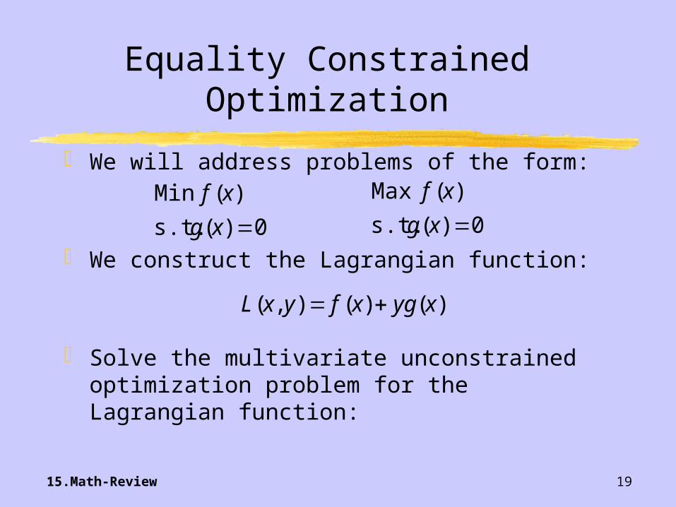
We will address problems of the form:

We construct the Lagrangian function:

Solve the multivariate unconstrained optimization problem for the Lagrangian function:

Equality Constrained Optimization

0)( s.t.

)(Min

xg

xf

)()(),( xygxfyxL

0)( s.t.

)(Max

xg

xf

15.Math-Review 20

We look for x and y that satisfy the 1st order optimality conditions for L(x,y):

under appropriate conditions on f(x) and g(x) the 1st order conditions of the Lagrangian are enough to guarantee optimality.

Equality Constrained Optimization

0)(

0)(')('

xg

xygxf

15.Math-Review 21

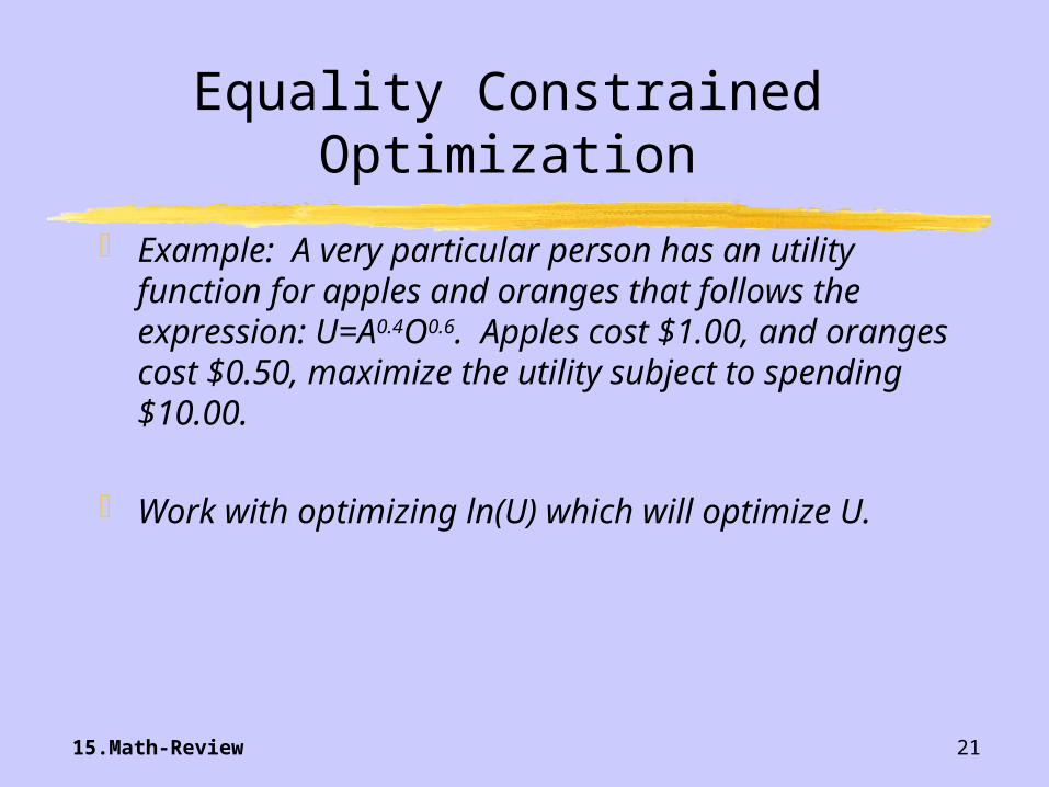
Example: A very particular person has an utility function for apples and oranges that follows the expression: U=A0.4O0.6. Apples cost $1.00, and oranges cost $0.50, maximize the utility subject to spending $10.00.

Work with optimizing ln(U) which will optimize U.

Equality Constrained Optimization

15.Math-Review 22

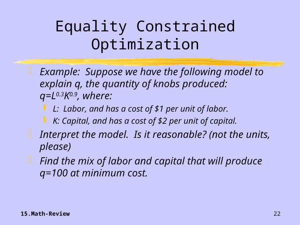
Example: Suppose we have the following model to explain q, the quantity of knobs produced: q=L0.3K0.9, where: L: Labor, and has a cost of $1 per unit of labor. K: Capital, and has a cost of $2 per unit of capital.

Interpret the model. Is it reasonable? (not the units, please)

Find the mix of labor and capital that will produce q=100 at minimum cost.

Equality Constrained Optimization