1 11 Simple Linear Regression and Correlation 11-1 Empirical Models 11-2 Simple Linear Regression...
60
1 11 Simple Linear Regression and Correlation CHAPTER OUTLINE Chapter 11 Table of Contents
-
Upload
lydia-gilbert -
Category
Documents
-
view
236 -
download
2
Transcript of 1 11 Simple Linear Regression and Correlation 11-1 Empirical Models 11-2 Simple Linear Regression...

1
11Simple Linear Regression and Correlation
CHAPTER OUTLINE
Chapter 11 Table of Contents

© John Wiley & Sons, Inc. Applied Statistics and Probability for Engineers, by Montgomery and Runger.
Learning Objectives for Chapter 11After careful study of this chapter, you should be able to do the
following:1. Use simple linear regression for building empirical models to engineering
and scientific data.2. Understand how the method of least squares is used to estimate the
parameters in a linear regression model.3. Analyze residuals to determine if the regression model is an adequate fit
to the data or to see if any underlying assumptions are violated.4. Test the statistical hypotheses and construct confidence intervals on the
regression model parameters.5. Use the regression model to make a prediction of a future observation and
construct an appropriate prediction interval on the future observation.6. Apply the correlation model.7. Use simple transformations to achieve a linear regression model.
2Chapter 11 Learning Objectives
© John Wiley & Sons, Inc. Applied Statistics and Probability for Engineers, by Montgomery and Runger.
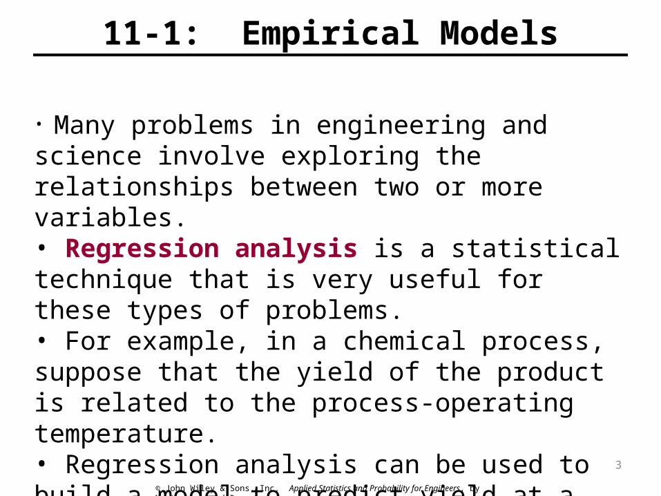
11-1: Empirical Models
• Many problems in engineering and science involve exploring the relationships between two or more variables. • Regression analysis is a statistical technique that is very useful for these types of problems. • For example, in a chemical process, suppose that the yield of the product is related to the process-operating temperature. • Regression analysis can be used to build a model to predict yield at a given temperature level.
3

© John Wiley & Sons, Inc. Applied Statistics and Probability for Engineers, by Montgomery and Runger.
11-1: Empirical Models
4

© John Wiley & Sons, Inc. Applied Statistics and Probability for Engineers, by Montgomery and Runger.
11-1: Empirical Models
Figure 11-1 Scatter Diagram of oxygen purity versus hydrocarbon level from Table 11-1. 5

© John Wiley & Sons, Inc. Applied Statistics and Probability for Engineers, by Montgomery and Runger.
11-1: Empirical Models
Based on the scatter diagram, it is probably reasonable to assume that the mean of the random variable Y is related to x by the following straight-line relationship:
where the slope and intercept of the line are called regression coefficients.The simple linear regression model is given by
where is the random error term.
6
© John Wiley & Sons, Inc. Applied Statistics and Probability for Engineers, by Montgomery and Runger.
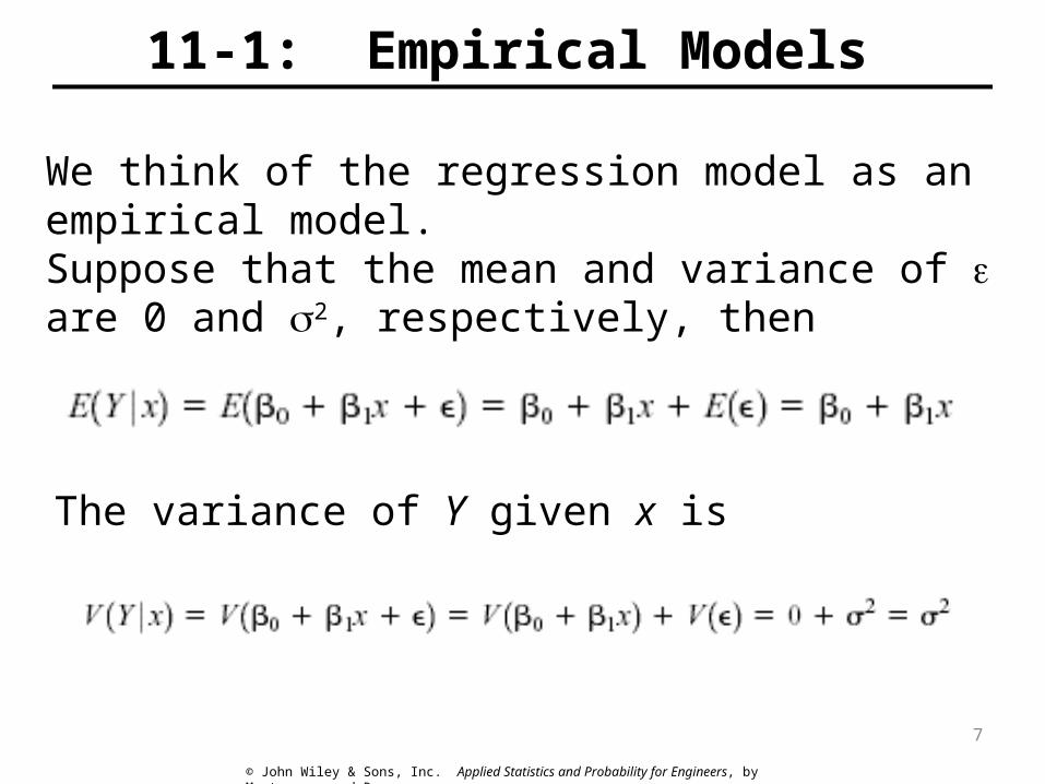
11-1: Empirical Models
We think of the regression model as an empirical model.Suppose that the mean and variance of are 0 and 2, respectively, then
The variance of Y given x is
7

© John Wiley & Sons, Inc. Applied Statistics and Probability for Engineers, by Montgomery and Runger.
11-1: Empirical Models
• The true regression model is a line of mean values:
where 1 can be interpreted as the change in the mean of Y for a unit change in x.• Also, the variability of Y at a particular value of x is determined by the error variance, 2.• This implies there is a distribution of Y-values at each x and that the variance of this distribution is the same at each x.
8

© John Wiley & Sons, Inc. Applied Statistics and Probability for Engineers, by Montgomery and Runger.
11-1: Empirical Models
Figure 11-2 The distribution of Y for a given value of x for the oxygen purity-hydrocarbon data.
9

© John Wiley & Sons, Inc. Applied Statistics and Probability for Engineers, by Montgomery and Runger.
11-2: Simple Linear Regression
• The case of simple linear regression considers a single regressor or predictor x and a dependent or response variable Y.• The expected value of Y at each level of x is a random variable:
• We assume that each observation, Y, can be described by the model
10

© John Wiley & Sons, Inc. Applied Statistics and Probability for Engineers, by Montgomery and Runger.
11-2: Simple Linear Regression
• Suppose that we have n pairs of observations (x1, y1), (x2, y2), …, (xn, yn).
Figure 11-3 Deviations of the data from the estimated regression model.
11

© John Wiley & Sons, Inc. Applied Statistics and Probability for Engineers, by Montgomery and Runger.
11-2: Simple Linear Regression
• The method of least squares is used to estimate the parameters, 0 and 1 by minimizing the sum of the squares of the vertical deviations in Figure 11-3.
Figure 11-3 Deviations of the data from the estimated regression model.
12
© John Wiley & Sons, Inc. Applied Statistics and Probability for Engineers, by Montgomery and Runger.
11-2: Simple Linear Regression
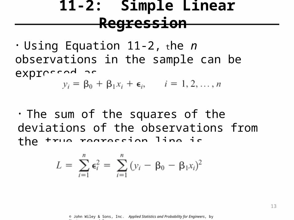
• Using Equation 11-2, the n observations in the sample can be expressed as
• The sum of the squares of the deviations of the observations from the true regression line is
13

© John Wiley & Sons, Inc. Applied Statistics and Probability for Engineers, by Montgomery and Runger.
11-2: Simple Linear Regression
14

© John Wiley & Sons, Inc. Applied Statistics and Probability for Engineers, by Montgomery and Runger.
11-2: Simple Linear Regression
15

© John Wiley & Sons, Inc. Applied Statistics and Probability for Engineers, by Montgomery and Runger.
11-2: Simple Linear Regression
Definition
16

© John Wiley & Sons, Inc. Applied Statistics and Probability for Engineers, by Montgomery and Runger.
11-2: Simple Linear Regression
17
© John Wiley & Sons, Inc. Applied Statistics and Probability for Engineers, by Montgomery and Runger.
11-2: Simple Linear Regression
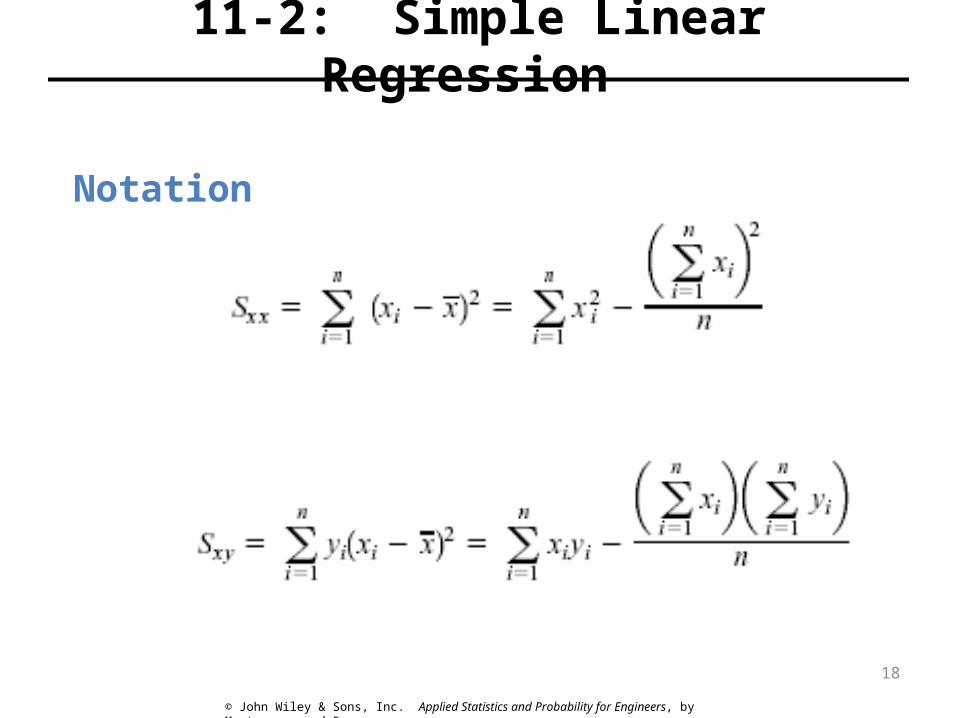
Notation
18

© John Wiley & Sons, Inc. Applied Statistics and Probability for Engineers, by Montgomery and Runger.
11-2: Simple Linear Regression Example 11-1
19

© John Wiley & Sons, Inc. Applied Statistics and Probability for Engineers, by Montgomery and Runger.
11-2: Simple Linear Regression
Example 11-1
20

© John Wiley & Sons, Inc. Applied Statistics and Probability for Engineers, by Montgomery and Runger.
11-2: Simple Linear Regression
Example 11-1
Figure 11-4 Scatter plot of oxygen purity y versus hydrocarbon level x and regression model ŷ = 74.20 + 14.97x.
21

© John Wiley & Sons, Inc. Applied Statistics and Probability for Engineers, by Montgomery and Runger.
11-2: Simple Linear Regression
Example 11-1
22

© John Wiley & Sons, Inc. Applied Statistics and Probability for Engineers, by Montgomery and Runger.
23
© John Wiley & Sons, Inc. Applied Statistics and Probability for Engineers, by Montgomery and Runger.
11-2: Simple Linear Regression
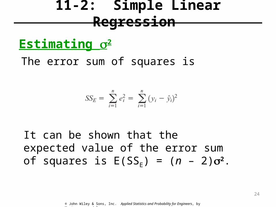
Estimating 2
The error sum of squares is
It can be shown that the expected value of the error sum of squares is E(SSE) = (n – 2)2.
24

© John Wiley & Sons, Inc. Applied Statistics and Probability for Engineers, by Montgomery and Runger.
11-2: Simple Linear Regression
Estimating 2
An unbiased estimator of 2 is
where SSE can be easily computed using
25

© John Wiley & Sons, Inc. Applied Statistics and Probability for Engineers, by Montgomery and Runger.
11-3: Properties of the Least Squares Estimators
• Slope Properties
• Intercept Properties
26
© John Wiley & Sons, Inc. Applied Statistics and Probability for Engineers, by Montgomery and Runger.
11-4: Hypothesis Tests in Simple Linear Regression
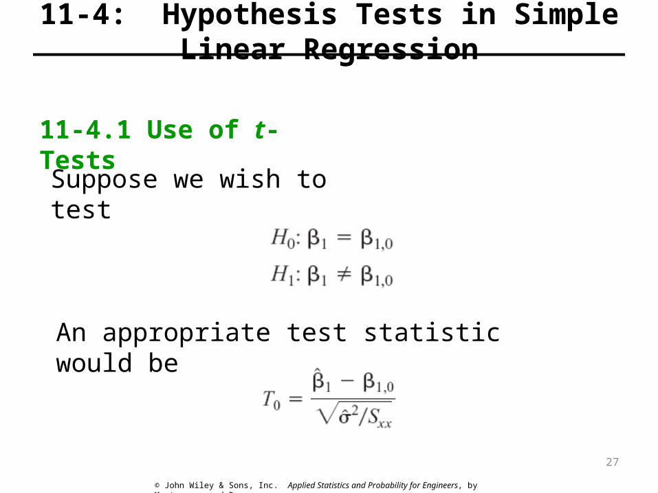
11-4.1 Use of t-Tests
Suppose we wish to test
An appropriate test statistic would be
27

© John Wiley & Sons, Inc. Applied Statistics and Probability for Engineers, by Montgomery and Runger.
11-4: Hypothesis Tests in Simple Linear Regression
11-4.1 Use of t-Tests
We would reject the null hypothesis if
The test statistic could also be written as:
28

© John Wiley & Sons, Inc. Applied Statistics and Probability for Engineers, by Montgomery and Runger.
11-4: Hypothesis Tests in Simple Linear Regression
11-4.1 Use of t-Tests
Suppose we wish to test
An appropriate test statistic would be
29

© John Wiley & Sons, Inc. Applied Statistics and Probability for Engineers, by Montgomery and Runger.
11-4: Hypothesis Tests in Simple Linear Regression
11-4.1 Use of t-Tests
We would reject the null hypothesis if
30

© John Wiley & Sons, Inc. Applied Statistics and Probability for Engineers, by Montgomery and Runger.
11-4: Hypothesis Tests in Simple Linear Regression
11-4.1 Use of t-Tests
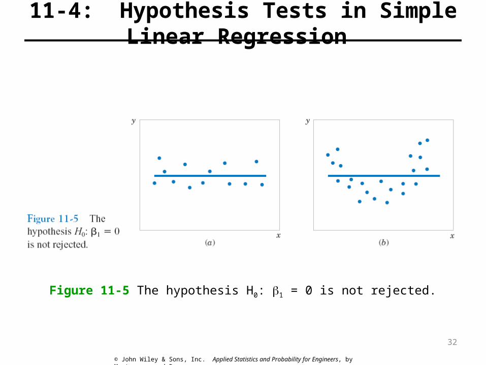
An important special case of the hypotheses of Equation 11-18 is
These hypotheses relate to the significance of regression.Failure to reject H0 is equivalent to concluding that there is no linear relationship between x and Y.
31
© John Wiley & Sons, Inc. Applied Statistics and Probability for Engineers, by Montgomery and Runger.
11-4: Hypothesis Tests in Simple Linear Regression
Figure 11-5 The hypothesis H0: 1 = 0 is not rejected.
32

© John Wiley & Sons, Inc. Applied Statistics and Probability for Engineers, by Montgomery and Runger.
11-4: Hypothesis Tests in Simple Linear Regression
Figure 11-6 The hypothesis H0: 1 = 0 is rejected.
33
© John Wiley & Sons, Inc. Applied Statistics and Probability for Engineers, by Montgomery and Runger.
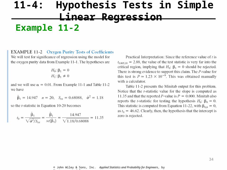
11-4: Hypothesis Tests in Simple Linear Regression
Example 11-2
34

© John Wiley & Sons, Inc. Applied Statistics and Probability for Engineers, by Montgomery and Runger.
11-4: Hypothesis Tests in Simple Linear Regression
11-4.2 Analysis of Variance Approach to Test Significance of Regression
The analysis of variance identity is
Symbolically,
35
© John Wiley & Sons, Inc. Applied Statistics and Probability for Engineers, by Montgomery and Runger.
11-4: Hypothesis Tests in Simple Linear Regression
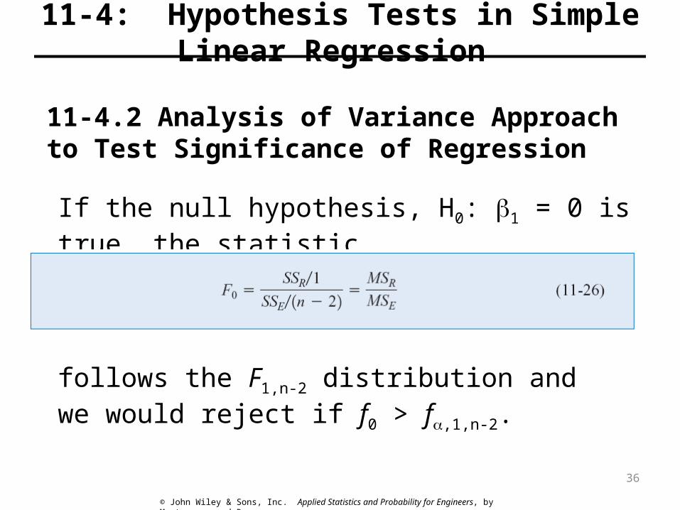
11-4.2 Analysis of Variance Approach to Test Significance of Regression
If the null hypothesis, H0: 1 = 0 is true, the statistic
follows the F1,n-2 distribution and we would reject if f0 > f,1,n-2.
36

© John Wiley & Sons, Inc. Applied Statistics and Probability for Engineers, by Montgomery and Runger.
11-4: Hypothesis Tests in Simple Linear Regression
11-4.2 Analysis of Variance Approach to Test Significance of Regression
The quantities, MSR and MSE are called mean squares.Analysis of variance table:
37

© John Wiley & Sons, Inc. Applied Statistics and Probability for Engineers, by Montgomery and Runger.
11-4: Hypothesis Tests in Simple Linear Regression
Example 11-3
38
© John Wiley & Sons, Inc. Applied Statistics and Probability for Engineers, by Montgomery and Runger.
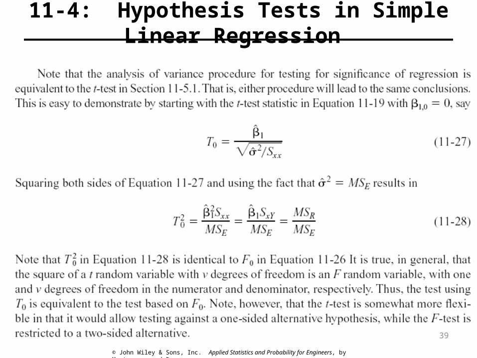
11-4: Hypothesis Tests in Simple Linear Regression
39

© John Wiley & Sons, Inc. Applied Statistics and Probability for Engineers, by Montgomery and Runger.
11-5: Confidence Intervals
11-5.1 Confidence Intervals on the Slope and Intercept
Definition
40

© John Wiley & Sons, Inc. Applied Statistics and Probability for Engineers, by Montgomery and Runger.
11-5: Confidence Intervals
Example 11-4
41

© John Wiley & Sons, Inc. Applied Statistics and Probability for Engineers, by Montgomery and Runger.
11-5: Confidence Intervals
11-5.2 Confidence Interval on the Mean Response
Definition
42

© John Wiley & Sons, Inc. Applied Statistics and Probability for Engineers, by Montgomery and Runger.
11-5: Confidence Intervals Example 11-5
43
© John Wiley & Sons, Inc. Applied Statistics and Probability for Engineers, by Montgomery and Runger.
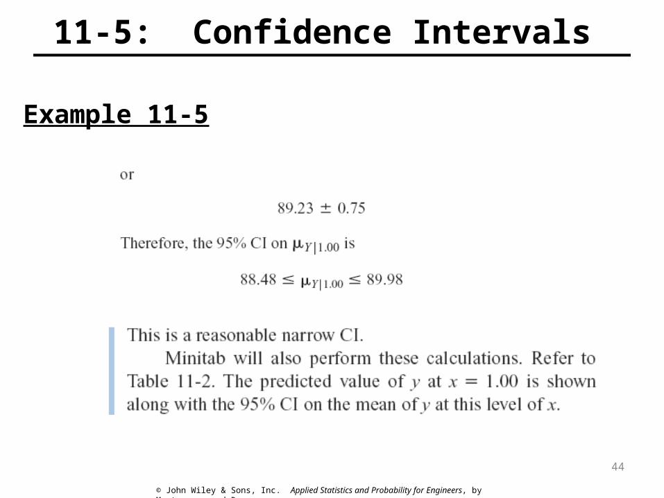
11-5: Confidence Intervals
Example 11-5
44

© John Wiley & Sons, Inc. Applied Statistics and Probability for Engineers, by Montgomery and Runger.
11-5: Confidence Intervals
Example 11-5
45

© John Wiley & Sons, Inc. Applied Statistics and Probability for Engineers, by Montgomery and Runger.
11-5: Confidence Intervals
Figure 11-7
Figure 11-7 Scatter diagram of oxygen purity data from Example 11-1 with fitted regression line and 95 percent confidence limits on Y|x0.
46

© John Wiley & Sons, Inc. Applied Statistics and Probability for Engineers, by Montgomery and Runger.
11-6: Prediction of New Observations
If x0 is the value of the regressor variable of interest,
is the point estimator of the new or future value of the response, Y0.
47

© John Wiley & Sons, Inc. Applied Statistics and Probability for Engineers, by Montgomery and Runger.
11-6: Prediction of New Observations
Definition
48

© John Wiley & Sons, Inc. Applied Statistics and Probability for Engineers, by Montgomery and Runger.
11-6: Prediction of New Observations
Example 11-6
49

© John Wiley & Sons, Inc. Applied Statistics and Probability for Engineers, by Montgomery and Runger.
11-6: Prediction of New Observations
Example 11-6
50

© John Wiley & Sons, Inc. Applied Statistics and Probability for Engineers, by Montgomery and Runger.
11-6: Prediction of New Observations
Figure 11-8
Figure 11-8 Scatter diagram of oxygen purity data from Example 11-1 with fitted regression line, 95% prediction limits (outer lines) , and 95% confidence limits on Y|x0.
51

© John Wiley & Sons, Inc. Applied Statistics and Probability for Engineers, by Montgomery and Runger.
11-7: Adequacy of the Regression Model
• Fitting a regression model requires several assumptions.1. Errors are uncorrelated random variables with
mean zero;2. Errors have constant variance; and,3. Errors be normally distributed.
• The analyst should always consider the validity of these assumptions to be doubtful and conduct analyses to examine the adequacy of the model
52

© John Wiley & Sons, Inc. Applied Statistics and Probability for Engineers, by Montgomery and Runger.
11-7: Adequacy of the Regression Model
11-7.1 Residual Analysis
• The residuals from a regression model are ei = yi - ŷi , where yi is an actual observation and ŷi is the corresponding fitted value from the regression model. • Analysis of the residuals is frequently helpful in checking the assumption that the errors are approximately normally distributed with constant variance, and in determining whether additional terms in the model would be useful.
53

© John Wiley & Sons, Inc. Applied Statistics and Probability for Engineers, by Montgomery and Runger.
11-7: Adequacy of the Regression Model
11-7.1 Residual Analysis
Figure 11-9 Patterns for residual plots. (a) satisfactory, (b) funnel, (c) double bow, (d) nonlinear. [Adapted from Montgomery, Peck, and Vining (2006).]
54

© John Wiley & Sons, Inc. Applied Statistics and Probability for Engineers, by Montgomery and Runger.
11-7: Adequacy of the Regression Model
Example 11-7
55

© John Wiley & Sons, Inc. Applied Statistics and Probability for Engineers, by Montgomery and Runger.
11-7: Adequacy of the Regression Model
Example 11-7
56

© John Wiley & Sons, Inc. Applied Statistics and Probability for Engineers, by Montgomery and Runger.
11-7: Adequacy of the Regression Model
Example 11-7
Figure 11-10 Normal probability plot of residuals, Example 11-7.
57

© John Wiley & Sons, Inc. Applied Statistics and Probability for Engineers, by Montgomery and Runger.
11-7: Adequacy of the Regression Model
Example 11-7
Figure 11-11 Plot of residuals versus predicted oxygen purity, ŷ, Example 11-7.
58

© John Wiley & Sons, Inc. Applied Statistics and Probability for Engineers, by Montgomery and Runger.
11-7: Adequacy of the Regression Model
11-7.2 Coefficient of Determination (R2)
• The quantity
is called the coefficient of determination and is often used to judge the adequacy of a regression model.• 0 R2 1;• We often refer (loosely) to R2 as the amount of variability in the data explained or accounted for by the regression model.
59

© John Wiley & Sons, Inc. Applied Statistics and Probability for Engineers, by Montgomery and Runger.
11-7: Adequacy of the Regression Model
11-7.2 Coefficient of Determination (R2)
• For the oxygen purity regression model, R2 = SSR/SST
= 152.13/173.38 = 0.877
• Thus, the model accounts for 87.7% of the variability in the data.
60