Institut de Recerca en Economia Aplicada Regional i Pública Document de Treball 2021/01 1/72 pág. Research Institute of Applied Economics Working Paper 2021/01 1/72 pág.

“Mixed Oligopoly and Market Power Mitigation: Evidence from the Colombian Wholesale Electricity Market”

Carlos Suarez

4

WEBSITE: www.ub.edu/irea/ • CONTACT: irea@ub.edu

The Research Institute of Applied Economics (IREA) in Barcelona was founded in 2005, as a research

institute in applied economics. Three consolidated research groups make up the institute: AQR, RISK

and GiM, and a large number of members are involved in the Institute. IREA focuses on four priority

lines of investigation: (i) the quantitative study of regional and urban economic activity and analysis of

regional and local economic policies, (ii) study of public economic activity in markets, particularly in the

fields of empirical evaluation of privatization, the regulation and competition in the markets of public

services using state of industrial economy, (iii) risk analysis in finance and insurance, and (iv) the

development of micro and macro econometrics applied for the analysis of economic activity, particularly

for quantitative evaluation of public policies.

IREA Working Papers often represent preliminary work and are circulated to encourage discussion.

Citation of such a paper should account for its provisional character. For that reason, IREA Working

Papers may not be reproduced or distributed without the written consent of the author. A revised version

may be available directly from the author.

Any opinions expressed here are those of the author(s) and not those of IREA. Research published in

this series may include views on policy, but the institute itself takes no institutional policy positions.

Abstract

Using information on price bids in wholesale electricity pools and empirical techniques described in the literature on electricity markets, this study identifies the market power mitigation effect of public firms in the Colombian market. The results suggest that while private firms exercise less market power than is predicted by a profit-maximization model, there are marked differences between private and public firms in their exercise of unilateral market power. These findings support the hypothesis of the market power mitigation effect of public firms.

JEL classification: L13, L94, C10. Keywords: Electricity Markets, Market Power, Privatization, Mixed Oligopoly, Regulatory Intervention.

Carlos Suarez: Department of Econometrics, Statistics and Applied Economics, Research Group on Governments and Markets, University of Barcelona, Avinguda Diagonal 690, 08034 Barcelona, Tower 6 Floor 3. Engineering Department, Research Group on Energy, Environment and Development, Jorge Tadeo Lozano University. Email: casuarez1978@gmail.com

1 Introduction

A key concern in any discussion about privatization is the benefits that might accrue to

society from public firms. Their advocates claim that they can be used as economic policy

instruments. In mixed oligopoly markets (i.e., markets in which private and public firms

compete), some economists and policy-makers argue that public enterprises are able to

mitigate market power through more competitive pricing, or what I shall refer to here

as “regulatory intervention”.1

The mixed oligopoly literature has analyzed the strategic interaction between public

and private firms in non-perfect competitive markets in order to establish, in theory, the

welfare e↵ects of privatization. Several studies employing such models have concluded

that full privatization is inadvisable because it can have counter-competitive e↵ects on

the market and lead to subsequent increases in terms of deadweight loss (De Fraja and

Delbono, 1989; Matsumura, 1998). These conclusions arise from the assumption that

the objective function of public and mixed firms di↵ers from that of private firms. In

most cases, mixed oligopoly models assume that private firms aim to maximize profits

while the objective function of public (or mixed) firms is to promote social welfare.2

Public firms may have objectives other than profit maximization and may even have a

multiplicity of objectives (Kay and Thompson, 1986).3 In the field, the objective function

of this type of firm depends on several issues related to the government’s ultimate goal

and the incentives provided to their managers (Fershtman and Judd, 1987) and it is thus

not possible to know a priori what the objective function of a public firm is.4

1In this paper, public firms are defined as those in which national or local governments have amajority shareholding and control their management.

2Traditional approaches to public firms have mainly viewed them as instruments of governmentpolicy and planning (Bos, 2015). Following this approach, the mixed oligopoly model assumes that theobjective functions of public firms is to promote social welfare.

3According to Kay and Thompson (1986), “Public sector managers could be expected to respond to

the particular personal incentives with which they were faced. Such incentives might lead to a desire to

maximise the scale of operations of the business, subject to any external financial constraint, or to seek

a quiet life untroubled by changes in working practices or di�culties in labour relations, rather than to

pursue a nebulous public good.”4For instance, if there is political pressure from voters to decrease prices, public firms may try

to mitigate market power, even applying predatory prices. Conversely, if a government is seeking toredress a fiscal deficit, its state-owned firms may try to maximize profits using market power markups

1

Given this ambiguity, and its obvious importance in determining the e↵ect of private

and state ownership on competition, the behavioral di↵erence between public and private

firms is a matter that merits empirical analysis.

The possibility of conducting such analyses in regulated industries has been greatly

enhanced over the last three decades thanks to the improved availability of data and a

diversity of market reforms. As a result of these two developments, it is now possible to

empirically address the key question underpinning the mixed oligopoly model, namely:

Do public and private firms behave the same when faced with equivalent incentives? An

empirical analysis of di↵erences in the way in which private and public firms exercise

their market power should provide interesting insights.

In this paper, I address the strategic pricing of public and private firms from an empir-

ical perspective in order to determine how they exercise their market power. Specifically,

I extend the analysis of the incentive to exercise market power (IEMP), as proposed by

McRae and Wolak (2009), to the case of two di↵erent types of firm showing disparate be-

havior in response to the same strategic incentives. This technique draws on information

about individual bids (willingness to sell) available in the electricity markets organized as

a multi-product auction. I apply this extended methodology to the Colombian wholesale

electricity market.

The case of the Colombian electricity market is appealing because market power

and marked rises in wholesale electricity prices are a major concern for the Colombian

authorities, consumers, and stakeholders alike. Leading industrial consumers tend to

be well organized and lobby the government for energy cost reductions. At the same

time, the Ministry of Energy and Mines sits on the board of several of the leading public

electricity generation companies. As a result, there are potential incentives for public

and mixed firms under government control to exert market power mitigation.5

as a covert form of taxation. Likewise, governments committed to a privatization program will boost apublic firm’s profit performance in order to increase the sale price. In addition, in the particular case ofmixed firms with a government majority share, the board members have a fiduciary duty to the minorityshareholders and therefore cannot ignore profit-maximization incentives. I owe this observations to ananonymous referee.

5It is important to clarify that, in relation to the objective function of public companies in theColombian wholesale electricity market, in this document I try to establish how close their price responses

2

Besides its relationship to mixed oligopoly models, this paper also lies at the inter-

section of two other di↵erent strands in the literature: i) Empirical studies comparing

the e�ciency of public and private firms, and ii) studies estimating market power in

electricity markets.

To date, empirical studies of the e�ciency of public and private firms have focused pri-

marily on di↵erences in the performance (or productive e�ciency) of public and private

monopolies (Bel et al., 2010; Frydman et al., 1999; La Porta and Lopez-de Silanes, 1999;

Netter and Megginson, 2001). One relevant exception is the study by Seim and Waldfo-

gel (2013) which was specifically aimed at determining the goals implicit in the decisions

of public enterprises. Seim and Waldfogel (2013) estimated a spatial model of demand

based on information about Pennsylvania’s state liquor retailing monopoly and found

that the store network is very similar in size and configuration to the welfare-maximizing

configuration. My research is similarly focused on disentangling the di↵erences between

the goals of public and private firms, but it di↵ers from their study in that I analyze a

situation in which private and public companies compete in the same electricity market,

whereas Seim and Waldfogel (2013) investigated the goals of a public monopoly. To the

best of my knowledge, the only paper to focus on the di↵erences between public and

private firms competing in the same market is that by Barros and Modesto (1999), on

the Portuguese banking sector.

The economic literature examining the problem of market power in electricity gen-

eration markets is extensive. However, three main groups of empirical models can be

identified according to the methodological approach employed. The first of these is based

on the direct or indirect estimate of Lerner indexes or markups (Wolak, 2003; Wolfram,

1999). The second group of studies seeks to determine the agents’ market power, simulat-

ing the equilibrium conditions that emerge from economic models of oligopoly (Bushnell

et al., 2008; Green and Newbery, 1992; Hortacsu and Puller, 2008; Sweeting, 2007; Wolak,

are to the theoretical behavioral benchmarks proposed by the mixed oligopoly models. Rather thanevaluating whether public companies deploy a welfare-maximizing strategy, I evaluate whether or notpublic companies ignore their incentives to exercise market power. Although ignoring such incentivesis consistent with welfare maximization, there are other plausible theoretical benchmarks that couldexplain this behavior.

3

2000). The third approach involves the use of structural econometric models to estimate

functional or behavioral parameters (Reguant, 2014; Wolak, 2007; Wolfram, 1998).

Although several techniques have been proposed for estimating market power in elec-

tricity markets, few studies have attempted to distinguish di↵erences in competitive

behavior between heterogeneous types of firm. In this respect, my approach is related

to the studies by Hortacsu and Puller (2008) and Hortacsu et al. (2019), who examined

the bidding behavior of firms in the Texas electricity spot market and found di↵erences

in the competitive strategies of large and small firms. Concerning the methodological

approach, as mentioned above, my empirical implementation is similar to the estimation

model proposed by McRae and Wolak (2009).

The main contribution of this paper is the development of an empirical model to

analyze di↵erences between private and public firms in terms of their incentives to ex-

ercise market power in a multi-unit auction framework. This methodology provides a

new analytical tool that serves to clarify the e↵ect of mixed (private-state) ownership

on competition. Overall, this methodology is applicable to any multi-unit, uniform price

auction in which the competitors’ bids and marginal costs are observable.

The empirical analysis performed here suggests that there are marked di↵erences in

the way private and public firms exercise their unilateral market power, supporting the

hypothesis of the latter’s market power mitigation. The results indicate that public firms

do not price strategically in the spot market. Moreover, partial evidence was found to

suggest profit-maximization behavior on the part of private firms and of bidding under

the marginal cost pricing rule on the part of public firms. These findings are consistent

with the behavioral structure of mixed oligopoly models.

The rest of this paper is divided into five sections. Section two outlines the char-

acteristics of the Colombian wholesale electricity market and the structural problems

it presents that must be taken into account to accurately identify the behavioral pa-

rameters under study. Section three explains the theory underpinning the incentives for

profit-maximizing firms to exercise unilateral market power and stresses the di↵erences

in this regard with the behavior of firms that do not act strategically. This section also

4

describes the empirical approach adopted to identify the behavioral di↵erences between

private and public firms. Section four presents the data and the results of applying

the proposed empirical approach to this market and reports several robustness checks

on multiple econometric choices. The final section summarizes the results and presents

some conclusions.

2 The Colombian market and mixed competition

This section outlines the principal features of the Colombian electricity generation market

that distinguish it as a mixed oligopoly and describes the main elements of this market

that must be taken into account when examining problems of market power.

For a market to be considered a mixed oligopoly, it must satisfy three conditions: i)

the market must be liberalized, i.e. the price is determined by the competing bids made

by the producers; ii) public, private and mixed firms must compete in equal conditions,

i.e. there are no discrimination rules; and iii) the conditions of competition in the market

are not perfect, i.e. there are high levels of concentration.

As regards the first condition, since the introduction of the Public Utilities Act (Act

142 of 1994) and the Electricity Act (Act 143 of 1994), electricity generation in Colombia

has been organized as a pooled wholesale electricity market. Generators can sell their

energy by means of long-term bilateral contracts with other agents or directly in the

day-ahead power exchange. This exchange operates as a multi-unit, uniform first-price

auction, in which each generator reports a price bid (or willingness to sell) to the market

operator for each generation unit. With this information, and according to demand fore-

casts, the market operator organizes the generation units from the cheapest to the most

expensive (this arrangement is known as merit order) and defines the market clearing

price (spot price) for every hour of the day. This feature demonstrates that the Colom-

bian wholesale energy market is neither price-regulated nor a cost-based pool and that

it obeys the conditions of competition among producers.

Second, with respect to the coexistence of private and public companies in the Colom-

5

bian generation market, it should be noted that although the intention of the Colombian

electricity sector reform in the early nineties was to promote private entrepreneurship,

the activity has a high proportion of public or mixed firms under government control. It

is also important to clarify that classification of generation firms into “private” and “pub-

lic” categories in the Colombian electricity market is not direct because there are several

firms with both private and public participation. In addition, smaller publicly-owned

firms had power purchase agreements (PPAs) to buy electricity from privately-owned

generation plants. For the particular application reported here, this classification was

performed by unit, taking into account the category of shareholder controlling the firm

that represents the unit to the market operator.6

Table 1 shows market shares in the Colombian wholesale electricity market for 2014.

The second column reveals that four of the seven leading firms were state controlled in

that year according to the classification criterion adopted in this study. In consonance

with this information, the leading generation firms operating in Colombia during the

study period presented a heterogeneous ownership structure in terms of the private or

public nature of their major shareholders.

Table 1: Market shares in the Colombian electricity market - 2014

Firm Majority Shareholding Electricity Generation (gWh) % Cumulative %

EMGESA Private 13691 21% 21%EPM Public 13626 21% 42%

ISAGEN Public 10609 16% 59%GECELCA Public 7508 12% 71%COLINV. Private 6711 10% 81%

AES Private 3982 6% 87%GENSA Public 2436 4% 91%Others 5764 9% 100%Total 64328 100% 100%HH 1422

Source: XM - Market Operator

6It is important to consider that the entity responsible for the bidding process of a generation unit inthe Colombian wholesale electricity market is the firm that represents the unit to the market operator.Table D22 in appendix D presents the ownership features of the most important firms in the Colombianelectricity generation market and table D23 in appendix D lists the generator units used in the analysisand details the corresponding ownership group and classification into public or private.

6

Finally, as regards the third condition, i.e., the level of market competition and

concentration, electricity generation activity in Colombia shows levels of concentration

that correspond to a moderate oligopoly, according to the merger guidelines of the US

Department of Justice. Table 1 presents the participation of the six leading generation

companies in the Colombian generation market.

In addition to the above features, there are several other features of the Colombian

wholesale electricity market that must be considered in order to accurately characterize

the unilateral market power of electricity generators.

i Colombia’s generation supply is mainly produced by hydroelectric and thermoelectric

resources. In the case of the country’s hydro technology, it should be borne in mind

that Colombia’s rain regime is subject to the e↵ects of El Nino and La Nina events.

During the former, dry weather conditions have a negative impact on the contribu-

tion of hydroelectric resources, while the opposite occurs during La Nina events. In

addition, the annual rain regime fluctuates between a dry season (December, Jan-

uary, and February) and a wet one (April, May, and June). Daily information is

available on the river flows that feed the main hydro units. As for the country’s

thermal technology units, these are primarily gas and coal fired. The gas market in

Colombia is organized as a bilateral contract scheme, and the price of Colombia’s

main gas well was regulated during the study period. Likewise, the fees for using

the gas transport pipes are regulated according to a mixed scheme which takes into

consideration capacities and volumes alike. Information is available about the heat

rates of each thermoelectric plant. Table 2 highlights the importance of large hydro

plants and thermoelectric units.

ii Most energy transactions are performed through long-term, fixed-price forward con-

tracts. Since physical dispatch is centrally coordinated, bilateral forward contracts

work as financial hedges against spot prices (Garcia and Arbelaez, 2002). Generally,

information on transactions made through bilateral forward contracts is not available

in markets that are organized as a multi-product auction. An additional advantage

7

Table 2: Generation by type of resource - 2013 and 2014

Generation (gWh)Type December 2013 December 2014 Growth Share 2014Hydro 3622 3707 2% 68 %Thermal 1370 1474 8% 26 %

Small Units 300 305 2% 6%Cogeneration 32 45 41% 1%

Total 5323 5531 4% 100%Source: XM - Market Operator

of analyzing the case of the Colombian electricity market is that the information on

sales in long-term forward contracts is available after the market closes. Thus, the

net forward market position of the firms can be computed. Table 3 shows the total

energy traded in 2013 and 2014 in the electricity generation market, distinguish-

ing between transactions conducted through fixed-price forward contracts and direct

transactions in the day-ahead energy exchange.

Table 3: Energy sales by trade mechanism - 2013 and 2014

Generation (gWh)2013 2014 Growth Share 2014

Spot Market 14949 15507 4% 18%Forward Contracts 71374 69846 -2% 82%

Total 86323 85352 -1% 100%Source: XM - Market Operator

iii Finally, the rules of the Colombian electricity exchange market allow only one valid

bid price to be made per unit for each 24-hour period. For each unit participating

in the central dispatch, the bid consists of one bid price that remains valid for the

entire day and 24 quantities (commercial availability), one for each hour of the day.

The generators report these day-ahead bids in the market clearing period. Regard-

less of the fact that the market clears every hour (in order to account for di↵erences

in demand and in availability of non-centrally dispatched generation resources), the

generator can only bid one price and cannot change any part of its bid during the cor-

responding 24-hour period. This restriction has considerable implications as regards

incentives to exercise market power, as will be explained in detail in sub-section 3.1.

8

3 Theoretical background and identification

3.1 The incentives to exercise market power

This sub-section examines the theoretical background to an analysis of the IEMP of

profit-maximizing and non-strategic firms and the implications of certain features of

the Colombian wholesale electricity market regarding the identification approach. The

electricity market literature contains various empirical techniques for estimating market

power (Borenstein et al., 2002; Bushnell et al., 2008; Green and Newbery, 1992; Hortacsu

and Puller, 2008; Reguant, 2014; Wolak, 2003; Wolfram, 1998, 1999). A common element

in the most relevant papers conducting analyses of this type is that the estimation

strategy is based on the first order condition of the profit maximization problem. In

general, these order conditions make it possible to express the optimal price or bid as the

sum of a cost component plus a strategic component. Here, I adopt the model proposed

by Wolak (2000) and McRae and Wolak (2009). who have developed a methodology

for estimating the IEMP based on a simple model of profit-maximizing firms that have

ex-ante forward contract obligations in a residual demand setting. In this context, the

IEMP is the ability to change the spot price when withdrawing output with the aim

of maximizing profits. In a theoretical study, Allaz and Vila (1993) showed that when

profit-maximizing firms sell a large share of their output via forward contracts with fixed

prices, they have less incentive to increase prices on the spot markets.

According to McRae and Wolak (2009) model, assuming the generator has previously

sold an amount of energy qc

ihat a fixed price P c

ihby forward contracts, the profit function

of the generation firm i in the hour h can be defined by the following expression:

⇡ih = Ph(DRih)(DRih � qc

ih) + P

c

ihqc

ih� Ci(DRih)

where ⇡ih represents the profits of firm i in hour h in the electricity market, Ph is

the spot price, DRih is the residual demand of firm i in hour h, and Ci(DRih) is the

cost function of the firm i. From the first order condition, the following expression is

9

obtained:

Ph(DRih) =@Ci(DRih)

@DRih

�@Ph(DRih)

@DRih

(DRih � qc

ih)

| {z }strategic element

(1)

It should be borne in mind that at the point of market equilibrium, the residual

demand of firm i in hour h, DRih, is equal to the total quantity produced by that firm

in that hour, therefore @Ci(DRih)@DRih

is the marginal cost of firm i in hour h. This is the first

term of the right-hand side of equation 1; the second is the strategic element, i.e., its

IEMP, which is equal to the interaction of the inverse of the slope of the residual demand

curve and the firm’s net position in the forward contracts market. This interaction is

the optimal margin of a profit-maximizing firm. Thus, the more energy sold by the firm

through fixed-price forward contracts, the less the incentive to increase the spot price.

Note, however, that in cases in which the generator has an energy deficit relative to its

contractual commitments, it has the IEMP by reducing, as opposed to incrementing, the

spot price (McRae and Wolak, 2009).

Given the design of the Colombian wholesale electricity market, the daily bid con-

straint limits the generator’s ability to make the precise bid that will maximize its profit

function each hour. The generation firm must choose a single price in order to maxi-

mize its expected daily profits. This means it cannot bid a continuous supply function

that intersects the maximum profit points, given the di↵erent realizations of the residual

demand. Thus, hourly IEMPs are not necessarily the same as daily incentives.

To address this problem, I propose a daily measurement of the IEMP. This measure

can be used to express the first order condition of the daily profit maximization problem

as follows:7

s⇤

ijt= cijt +

�P

h2Hijt(DRith(sijt)� q

c

ith)

Ph2Hijt

@DRith(sijt)@sijt

(2)

where sijt is the daily bid price on day t for the energy of unit j, the asterisk highlights

7See appendix A for a derivation.

10

that this bid is optimal, cijt is the constant marginal cost of unit j, Hijt is defined as the

set of hours of day t where unit j is marginal, DRith is the residual demand of firm i

that owns unit j on day t at hour h and qc

ihis the energy previously sold at a fixed price

by firm i on day t. The second term on the right-hand side of equation 2 is a weighted

version of the inverse semi-elasticity of the residual demand. This is the IEMP of a firm

that maximizes daily expected profits. I compute the daily IEMP of the firms for the

daily model according to this expression.

From a behavioral perspective, strategic firms will take the IEMP into account in

their pricing, whereas non-strategic firms will not. However, what type of behavior can

be expected from public firms seeking to mitigate market power? Here, the theoretical

literature on mixed oligopolies o↵ers an appealing response. Beato and Mas-Colell (1984)

have demonstrated that public firms are able to restore market e�ciency by applying

the marginal cost pricing rule in a mixed oligopoly model in which public firms compete

with private firms, where the former are welfare maximizing and the latter are profit

maximizing. Hence, if public firms are implementing market power mitigation schemes,

we would expect them to apply the marginal cost pricing rule, or we would at least

expect the impact of the strategic element in prices to be less important for public than

for private firms.

What, therefore, are our expectations regarding public firms in the specific case of

Colombia? As stated in the introduction, there are potential incentives in Colombia

for public and mixed firms under government control to exert market power mitigation,

given the government’s direct participation on the board of several of these companies

and the capacity of interest groups to lobby for a reduction in electricity prices.

In sum, when private firms behave strategically, the interaction between the residual

demand slope and the net financial position has an impact on price bids. In contrast,

public firms have no IEMP, i.e., their prices are una↵ected by this interaction and are

primarily explained by the marginal cost.

11

3.2 Identification strategy and estimation

In this section, the di↵erences in the incentives for private and public firms to exercise

market power are addressed from an empirical perspective. The model presented here

adopts the estimation methodology proposed by McRae and Wolak (2009), but includes

the interaction between the firms’ type of ownership and their IEMP. The extension of

this model to establish these di↵erences in incentives is based on expression 2 for private

companies.

It is important to consider that my intention is to determine whether public and

private companies respond in the same way to incentives to exercise market power, and

therefore I require a strategy to test whether the supply functions of the di↵erent types

of company respond in di↵erent ways to changes in the inverse semi-elasticity of residual

demand. Note that the expression 2 can be interpreted as a behavioral supply function

of a profit-maximizing firm, while the marginal cost pricing rule can be interpreted as a

behavioral supply function of a firm that ignores its incentives to exercise market power.

Therefore, I assume that the behavioral supply of private and public companies is

given by the expression:

p⇤

ijtk= ✓cijt + ↵k ⇤

\IEMPijtk + ⌘ijtk (3)

Where ✓ is the passtthrough of marginal costs, cijt represents the marginal costs, ↵k

is the response to incentives to exercise market power of company i that owns unit j at

time t and which is of the nature k, k 2 {public, private}, \IEMPijtk is the estimate of

the incentives to exercise market power and finally ⌘ijtk is a measurement error in the

estimates of the incentives to exercise market power of firm i 8.

Note that the equation 2 is an equilibrium condition, therefore it is only valid for the

firm’s marginal bid. This implies that although all price bids can be observed in each

auction, those that are out of equilibrium do not necessarily fulfill the expression 2. Given

8Reguant (2014) notes the potential endogeneity and measurement error of the elastic strategiccomponent( markup term) in the empirical analog of the first-order condition of a profit-maximizingfirm.

12

the restrictions on the bidding program in the Colombian market described in section 2,

it is expected that the points of the bidding program outside a firm’s equilibrium will

show deviations from the optimality condition described by the expression 2. Each firms’

equilibrium quantities and bids arise from the interaction between the behavioral supply

function and the residual demand function; therefore, estimation of the parameter ↵k

implies a ”reverse causality” problem9.

In order to address this issue, it is necessary to adopt a simultaneous equations

approach and instrumentalize the IEMP. According to the interpretation of McRae and

Wolak (2009) the IEMP is equivalent to the inverse semi-elasticity of net residual demand

(After considering the previous forward contract obligations).

As regards the stochastic components of the residual demand, these can be generated

by demand shocks or by shifts in the competitors’ supply function. Consequently, I

will model the incentive to exercise market power (IEMP) as the sum of these two

components.

\IEMPijtk = ⌫th + ��ith (4)

It is reasonable to assume that the shocks of demand ⌫th come from expected and

unexpected consumer reactions which lie completely beyond the firms’ control. These

reactions may be a response to price changes (endogenous components) or to demand

driver changes (exogenous component)10. I will model the demand shocks as the sum of

expected changes to demand drivers,11 an elastic component which is clearly endogenous

and unexpected shocks which could be exogenous or endogenous.

9Note that the IEMP results from the expectations that various firms have about their rivals’ be-havior. According to the bid rules of the wholesale energy market, the competitors’ bids must be madesimultaneously. Thus, for generator A to estimate its residual demand curve, it has to form an expecta-tion about its rivals’ bid prices; however, at the same time, the bid prices of these rival firms will dependon their estimates of the residual demand curves, which in turn will be dependent on their expectationsregarding generator A’s bid prices.

10The fact that consumers’ reactions to demand driver changes are beyond the firms’ control suggestsindependence of these variables, rendering them candidates for suitable instruments.

11The demand drivers are external shocks that shift but do not rotate the inverse function of residualdemand

13

⌫th = ⇡1zth + ⇠th(pth) + �th (5)

Where ⇡1z1 represents the expected changes in demand drivers ⇠th(pt) represents

endogenous reaction to prices (elastic component) and �th is the sum of unexpected

demand shocks.

With regard to shocks in the competitors’ supply function, ��ith. These shifts may

be caused by foreseen changes in the costs of rival firms or by unforeseen impacts on

their strategic incentives (elastic component). Clearly, because this second component

depends on the strategic interaction of competing firms, poses a problem of endogeneity.

I will model the shocks in the competitors’ supply function as the sum of changes in rival

firms’ cost shifters ⇡2z2�ith

and the endogenous (and elastic) component !�ith(pt).

��ith = ⇡2z2�ith + !�ith(pth) (6)

Hence, plugging expressions (5) and (6) in expression (4), the IEMP can be expressed

as:

\IEMPijtk = ⇡1z1th + ⇡2z2�ith + ⇠th(pt) + !�ith(pt) + �th (7)

I address the endogeneity problem here by performing estimates that consider instru-

ments for the IEMP whose variation arises either from expected demand shocks z1th or

exclusively from the competitors’ cost component z2�ith (both of which are uncorrelalated

to the measurement error of the IEMP).

The literature on market power estimation in an environment of di↵erentiated prod-

ucts recommends using the observed characteristics of the products supplied by rival

firms in order to obtain the optimal instruments for a specific product (Berry et al.,

1995). By analogy, in the context of the electricity market, the instruments I have se-

lected are variables that are uncorrelated to the rivals’ elastic component but which at

the same time have e↵ects on their supply function, that is, factors associated with shifts

14

in the costs of rival firms 12 .

Specifically, I consider three instruments:

i A weekend day dummy variable is used in order to capture expected demand shocks;

this instrument is valid because it reasonable to assume that the weekday condition is

independent of the measurement error. Likewise, the only channel through which the

day of the week can a↵ect the supply of firm i is through a shift in the residual demand

curve. The cost shifters of electricity generation depend mainly on the technological

characteristics of the units and the cost of fuels. Generally, generating companies sign

long-term contracts for the supply of fuel, which do not include substantial changes

in the price of the same depending on the day of the week. The above suggests that

this instrument satisfies the exclusion restriction.

ii The inflows of the rivers feeding the rivals’ main hydraulic generation units are used

to account for changes in the marginal costs of the leading competitors. The indepen-

dent nature of this variable is evident given its dependency on natural phenomena.

Regarding the exclusion restriction, it is not expected that the inflows of the rivers

feeding the reservoirs of competitors have an impact on the opportunity cost of fuel

usage of the units of the firms owned by the firm i. Hence, shifts in residual demand

constitute the only pathway through which competitors’ river inflows can impact the

behavioral supply function.

iii The competitors’ full commercial availability, i.e., their total generation capacity on

specific days. It is important to clarify that in the Colombian wholesale electricity

market, commercial availability is the quantity component of the daily bid. Firms

can report only one commercial availability per unit for each hour. This availability

is taken into account by the regulator in order to calculate the historical unavailabil-

ity index due to forced fails. This indicator considers the observed unavailability of

each generation asset, and higher levels trigger a reduction in revenue from the gen-

12As instruments I use several rivals’ cost shifters which are equivalent to drivers of the residualdemand of firm i

15

eration back-up scheme under Colombian law (reliability charge). Thus, generation

companies do not have incentives to systematically make strategic use of commercial

availability. The greatest changes in this last variable are motivated by the scheduled

or unscheduled unavailability of the plants and by the highly variable contribution of

smaller base-load generation units. The short-term decisions of firm i do not have an

e↵ect on its competitors’ sources of variation and therefore, this variable can be con-

sidered independent. Likewise, the short-term contingencies or planned maintenance

intervention of rivals’ generation assets a↵ect neither the generation technology nor

the opportunity cost of fuel usage by the units owned by firm i. Hence, it is rea-

sonable to assume that the rivals’ commercial availability only a↵ects the behavioral

supply function through shifts in the residual demand.

Finally, in order to perform an estimation of the econometric model posed in ex-

pression (8), it is necessary to model the marginal cost component cijt. Marginal cost

estimates of the units can be obtained from engineering formulae and the technical char-

acteristics and prices of the observable inputs. However, there may be unit characteristics

and random shocks common to all plants that are not observable to the econometrician

and which have an e↵ect on marginal costs. In addition, it is important to bear in mind

that the computations performed to obtain the marginal cost estimate may contain a

measurement error given that fuel costs are approximated to reference prices, and the

cost per unit in actual fuel supply contracts may be di↵erent. Therefore, in this pa-

per it is assumed that the marginal costs of each unit can be expressed as the sum of

the marginal cost estimate based on the technical parameters of the unit, an individual

heterogeneity component and time e↵ect common to all the units, and an exogenous

disturbance term, i.e. cjt = bcjt + µj + 't + ⇣jt.

Thus, I estimate the following two-way fixed e↵ects linear regression model:

p⇤

ijt= �0 + ✓(bcijt) + ↵pri(D

pri

j⇤ \IEMPijt) + ↵pub(D

pub

j⇤ \IEMPijt) + µj + 't + "it (8)

16

where P⇤

ijtis the bid of firm i, for its marginal unit j on day t, ccijt is the estimate of the

marginal cost of unit j on day t, \IEMPijt is the estimation of the incentive to exercise

market power for a profit- maximizing firm (the empirical estimate of the second term of

the left-hand side of expression [2], for company i on day t for the hours in which unit j

was marginal, andDpub

jis a dummy variable that takes the value of 1 when unit j is owned

by a firm i under state control and 0 otherwise. Dpri

jis a dummy variable that takes the

value of 1 when unit j is owned by a private firm i and 0 otherwise. µj and 't represent

unobserved unit and time e↵ects, respectively. The term of disturbance "it contains the

unobservable exogenous disturbance term of the marginal cost and the sum of hourly

measurement errors of the IEMP, i.e., "it = ⇣jt + ⌘ijtk where ⌘ijtk =P24

h=1 ⌘ijthk. �0, ✓,

↵pub, ↵pri are the parameters to be estimated. This model is similar to the application

developed by McRae and Wolak (2009); however, in the present paper, heterogeneous

e↵ects are introduced for public and private companies.

It should be borne in mind that Pijt is the price-bid of unit j when the latter is

marginal. The first order condition expressed in equation 2 is not valid when unit j is

not marginal. This means that the panel data only contain information about those

plants that were marginal for at least one hour in the day. Likewise, in the case of the

residual demand approach, the marginal price bid of firm i is equal to the spot price,

that is, pth = s⇤

imt, if unit m is marginal in hour h. However, given the discontinuity and

ladder shape of the supply and residual demand functions, this does not always occur in

the real market. Therefore, there are two alternatives regarding the dependent variable

of the model presented in expression 8: Either the spot price when unit i clears the

market or the price bid of the marginal unit of each firm. Since a greater number of

observations can be used with the latter alternative (and unit j does not need to clear

the market), it can be considered the most appropriate option.

In the framework of the instrumental variables approximation, I implement several

specifications of the two-way fixed e↵ects proposed in expression 8. Note that for private

companies, the inclusion of these fixed e↵ects terms would allow them to bid prices

above or below the marginal cost independent of residual demand and their contractual

17

position, that is, for reasons independent of their IEMP. As far as public companies are

concerned, the additional fixed e↵ects would allow level-shift deviation, which implies

violating the marginal cost pricing rule.13 As I mentioned above, I interpret these fixed

e↵ects as unobservable individual heterogeneity and unobservable time e↵ect common

to all the units of the marginal cost. I assume that the unobservable, time-variant

heterogeneity of the marginal cost is orthogonal to the measurement error of the IEMP,

i.e., E⇥⇣0

jt⌘ijtk

⇤= 0.

I propose estimating the parameters ↵pub and ↵pri by implementing a linear general-

ized method of moments (GMM) model with standard errors clustered by unit. Assuming

a valid and relevant set of instruments Zijt, I am able to exploit the orthogonality con-

ditions of the instruments and the first order condition of the daily profit maximization

problem presented in expression 2 in order to construct the moments conditions. The

orthogonality conditions imply that:

E⇥Z

0

ijt"it

⇤= E

hZ

0

ijt

⇥P

⇤

ijt�✓(bcijt)�↵pri(Dpri

j· \IEMPijt)�↵pub(D

pub

j· \IEMPijt)�µj�'t

⇤i= 0

The parameters can now be estimated using the empirical analogue of these moments

conditions.

Finally, it is important to consider that estimation of the opportunity costs of using

hydro power resources involves dynamic components that do not necessarily correspond

to the first order conditions given in expression 2. For this reason, the baseline estima-

tions presented in this paper only uses data from situations in which the firms’ marginal

power plants use thermal technology.14 However, the importance of hydroelectric gen-

13I owe this observation to an anonymous referee.14Here, it is necessary to clarify that I do not include hydro units, not only because the opportunity

cost of water is di�cult to estimate, but also because for hydro units, the first-order condition for thistype of unit could be di↵erent from the one presented in expression (2). In the robustness check section,I present the results of the estimates including hydro units under the assumption of the same first-ordercondition for the di↵erent types of generation technology. The qualitative and quantitative results aresimilar to the baseline estimate.

18

eration in the Colombian electricity market is useful to refine the identification strategy

in order to address endogeneity issues.

The econometric exercises proposed here seek empirical evidence for the impact of

private and public companies’ IEMP in their bid prices according to the predictions of

the mixed oligopoly model. Three specific hypotheses are analyzed:

i Hypothesis 1 (H1): Given the same incentives, the exercise of market power by

state-owned and private firms di↵ers.

ii Hypothesis 2 (H2): Public firms (do not) exercise market power as non-strategic

agents, i.e. they apply the marginal cost pricing rule.

iii Hypothesis 3 (H3): Private firms exercise market power taking into account the

strategic element.

First, note that testing the null hypothesis, ↵pri = ↵pub in expression 8 is consonant

with the rationale that the exercise of market power by state-owned and private firms is

equal given their incentives. If private firms behave as profit maximizers and public en-

terprises implement market power mitigation schemes, then depending on the ownership

of each enterprise, the interaction of residual demand slope and net forward contract

position will impact di↵erently on their respective bidding strategies.

In the case of the second hypothesis, if public firms do not behave strategically, we

would expect the parameter ↵pub not to be statistically di↵erent from zero, i.e. null

hypothesis ↵pub = 0. If public firms exercise regulatory intervention, then their prices

will be explained mainly by the marginal cost and they will not be a↵ected by the

interaction of the residual demand and the net financial position.

Finally, according to theory, if private companies behave strategically (profit maxi-

mizers), we would expect the parameter ↵pri to be statistically significant and to present

a positive sign (being very close to 1 in the case of profit-maximizing firms), i.e. null

hypothesis ↵pri > 0 (↵pri = 1 in the case of profit maximization). If private firms behave

strategically, their IEMP has an impact on the firms’ pricing. These tests are performed

for each of the parameters estimated in the econometric models described above.

19

It is important to clarify that the interpretation of the coe�cient ↵ is di↵erent from

the conduct parameter ✓ estimated in several applications of the new empirical industrial

organization (NEIO) literature. First, the conduct parameter ✓ is an estimate of the

price-cost mark up adjusted by the elasticity of total demand. As this is corrected for

total demand, its interpretation is linked to the entire market competition model and not

to individual firm behavior. In the case of the parameter ↵, this can also be interpreted

as a measure of the price-cost mark up but adjusted by the elasticity of residual demand

and the percentage of exposure to the spot price of each firm. This measure is relative

to the best response of each particular firm.15

Interpretation of ↵ when it takes the values 0 or 1 is clear: When ↵ is 1, the firm is

maximizing its profit unilaterally in the static game, and when ↵ is 0, the firm is ignor-

ing its incentives to exercise market power (and potentially applying the marginal cost

pricing rule). However, when ↵ takes di↵erent values, interpretation is less clear as it is

not associated with stylized competitive behavior (profit maximization or competition).

Deviations from stylized behavior values may be interpreted in the same way as in

Hortacsu and Puller (2008) and Hortacsu et al. (2019), i.e., as deviations of optimization

behavior unrelated to strategic reasons. Alternatively, values of ↵ between 0 and 1 can

be interpreted as evidence that the firm is o↵ering prices as if it were facing a more elastic

residual demand than is the case, for strategic reasons. Mercadal (2019) posits that when

15The conduct parameter ✓ represents firms’ beliefs regarding how competitors will react to changes inthe firm’s quantity. Meanwhile, the parameter ↵ can be interpreted as a measure of the extent to whicha company adopts its best response strategy unilaterally given its own forward contracting and the bidsof its competitors. The parameter ↵ does not necessarily inform us about the underlying competitionmodel in the market (this parameter tells us nothing about the competitors’ best response); rather,it indicates whether each firm’s unilateral response is consistent with unilateral profit maximizationin the static model. It is important to clarify that I go beyond calculating the inverse elasticity oftotal demand using econometric methods. In this paper, the IEMP is in principle observed, and isestimated using a non-parametric method which considers the actual residual demand and includes thereaction of competitors to potential changes in the price bids of firm i. According to Corts (1999), ifeach firm i anticipates that its rivals’ aggregate output is a function Ri(qi) and if R0

i(qi) = ri, firm i ’sfirst-order condition is P = c

0i(qi) � (1 + ri)P 0(Q)qi, which is equivalent to (1) when ✓i = 1 + ri. In

terms of the notation used by Corts (1999), my regressor of interest, i.e., the IEMP, already includes thedirection of R0

i(qi). Given that I can observe the inverse semi-elasticity of demand, it is not necessary toconjecture about the competitive behavior of the competitors of firm i, because in the regression model,the parameter ↵ is not the coe�cient of �P

0(Q)qi, as in the case of the conduct parameter, but thecoe�cient of �(1� ri)P 0(Q)qi.

20

attempting to determine entry, generators do not play best response (in the static game),

but act as if they were facing a more elastic residual demand (This is ↵ < 0).16 On the

other hand, values of the parameter ↵ greater than 1 can be interpreted as evidence

that the firm is o↵ering prices as if it were facing a less elastic residual demand than it

actually does, for strategic reasons. Mercadal (2019) suggests that, in a repeated game

cooperative equilibrium, firms do not play best response, but instead behave as if they

were facing a less elastic residual demand than than they actually do (This is ↵ > 1).17

The section that follows describes the methodological procedure for computing the

model’s variables, including the IEMP and marginal costs. Finally, the econometric

method employed in the estimation is outlined and the most relevant results are pre-

sented.

4 Empirical Implementation

The hourly and daily data for 21 firms in the Colombian wholesale electricity market

were analyzed for the period 2005 to 2014. To test the three hypotheses (H1, H2, and

H3) by estimating the parameters ↵pub and ↵pri of the model proposed in expression 8,

we also need data on marginal costs and on the IEMP. Unfortunately, these variables

cannot be observed directly, so we have to rely on indirect estimations.

In the case of marginal costs, an accounting approach is adopted. This is similar to

16There may be several reasons for a firm to o↵er prices “as if it faced” a more elastic residual demand.For example, the firm may fear regulatory intervention to reduce unilateral market exercise, so it doesnot exercise its full market power when the resulting price increases could arouse excessive concern inthe authorities. Likewise, in the case of a public company seeking to balance consumer welfare andprofits, 1� ↵ could be interpreted as the importance that the firm gives to consumer welfare.

17Note that interpretations associated with entry deterrence, fear of regulatory intervention, andcooperative equilibrium implicitly entail scenarios of dynamic strategic interaction, namely, a profit-maximization model subject to an incentive compatibility constraint associated with future revenues.If the incentive compatibility constraints are a function of simultaneous residual demand shocks, thenthe estimated ↵ parameter may be subject to Corts (1999) criticism (i.e., ↵ may be biased). In anyevent, according to the identification strategy suggested by Puller (2009), the inclusion of time fixede↵ects in my base line estimation allows me to address this potential inconsistent estimation issue.According to Puller (2009), theoretically, the unobserved e↵ect related to the incentive compatibilityconstraint “is equal across all firms in the collusive regime for a given period (i.e., it is not indexed by

i). Although, a researcher does not have data on it, this extra term can be ‘conditioned out’ by including

time fixed-e↵ects”.

21

Figure 1: Estimated marginal costs

(a) Private units (b) Public units

Source: Data from XM - Calculations and elaboration: Author.

the one employed in previous studies in the field of electricity markets (Borenstein and

Bushnell, 1999; Borenstein et al., 2002; Fabra and Reguant, 2014; Green and Newbery,

1992; Wolak, 2000; Wolfram, 1998, 1999). The marginal costs of thermal plants are

computed, based on the technical parameters of the plants (heat rate), fuel costs, and

fuel transportation costs. The data sources and more detailed information concerning the

assumptions for the calculation and imputation of these costs are presented in appendix

B. It is important to bear in mind that these computations may contain a measurement

error given that I approximate fuel costs to reference prices, and the cost per unit in

actual fuel supply contracts may be di↵erent.

Daily marginal costs were calculated and imputed for 36 thermal plants belonging to

21 firms. Given the small di↵erences in heat rate between publicly owned and private

units, no significant di↵erences were found in the distribution of marginal costs between

public and private generation units. Panels (a) and (b) in figure 1 present the histograms

of the estimated marginal costs for private and public generation units, respectively.

As for the IEMP, recall that this incentive is related to the elasticity of residual

demand. Since the Colombian wholesale electricity market allows us to observe the price

bids and commercial availability of each plant as well as actual electricity demand, it is

possible to replicate the residual demand of each generator. The result of this exercise

is a decreasing step function of residual demand in which the partial derivative is zero

22

or indeterminate (McRae and Wolak, 2009). Therefore, to calculate the inverse net

semi-elasticity of demand, an approximation must be made to the slope of this function

around the market equilibrium price. Wolak (2003) suggests a non-parametric method

for calculating the elasticity of residual demand using the points of the function with

prices closest to — both above and below — the market equilibrium price.

As stated above, a daily version of the IEMP was computed to account for the fact

that in the Colombian electricity market, generators maximize daily as opposed to hourly

profits (see sub-section 3.1). Adopting the methodology proposed by Wolak (2003), the

empirical version of the IEMP — i.e., the second term on the right-hand side of equation

2 — can be computed as follows:

\IEMPijt =�P

(IGith � qc

ith|unit j is marginal in hour h)

P(DRith(pth·(1+�))�DRith(pth·(1��))

pabove

th(1+�)�p

below

th(1��)

|unit j is marginal in hour h)(9)

where \IEMPijt is the incentive to exercise market power on day t for unit j that is

marginal for several hours of the day, paboveth

(1 + �) is the price of the next step in the

residual demand curve above the price pth ·(1+�), pbelowth(1+�) is the price of the previous

step in the residual demand curve below the price pth · (1� �), IGith is the actual ideal

generation of producer i in hour h and qc

ithis the quantity of energy committed in fixed

price forward contracts.18 As stated in section 2, in the Colombian wholesale electricity

market this quantity is observable ex post. Finally, I assume a parameter � = 0.05 (5%).

Figure 2 illustrates this non-parametric calculation technique. Previous studies using

this methodology (McRae and Wolak, 2009; Wolak, 2000) suggest that changes in � do

not have a marked e↵ect on the outcomes. Later in this paper, in the robustness checks

section, I verify that the decision regarding the parameter � does not have a critical

impact on the results of the estimates. I present the estimates obtained by applying �

18From a supply function equilibrium approach (Klemperer and Meyer, 1989), the marginal price bidis the best response of an electricity generating firm given the actions taken by its competitors (as itsets its level of generation and the spot price). This optimal bid price is associated with an optimalgeneration quantity, so the residual demand of the generator in the equilibrium price should be equalto its ideal generation.

23

of 10% and 25% to compute \IEMPijt.

Figure 2: IEMP Calculation technique

Source: Data from XM - Calculations and elaboration: Author.

Information about daily price bids, hourly spot prices, hourly ideal generation and

hourly sales in forward contracts — essential details to compute the IEMP — was taken

from the website of the Colombian wholesale electricity market operator XM.

A shortcoming of the IEMP calculation technique presented above is that it can yield

extreme values due to absolute values close to zero in the denominator of expression 9.

In fact, in the sample analyzed in this paper, extreme values are obtained which can

reach 2.228 times the interquartile range. Panel (a) in figure 3 presents a scatter plot

for the IEMP and the margin (P ⇤

ijt� cjt) for the total sample in which extreme outliers

are present. In order to address this issue, the sample has been trimmed to exclude the

observations corresponding to the 1% lowest values for the denominator of expression

9, i.e., the sum of the slopes of the hourly residual demand functions. Panel b in figure

3 presents an IEMP vs. margin scatter plot, after trimming. In the robustness tests,

several trimming percentile values are tested but they have no major impact on results.

Unlike the situation with estimated costs, some di↵erences were found in the de-

scriptive statistics of the IEMP for private and public companies. Figure 4 shows the

distribution of the IEMP among the main public and private electricity generation com-

24

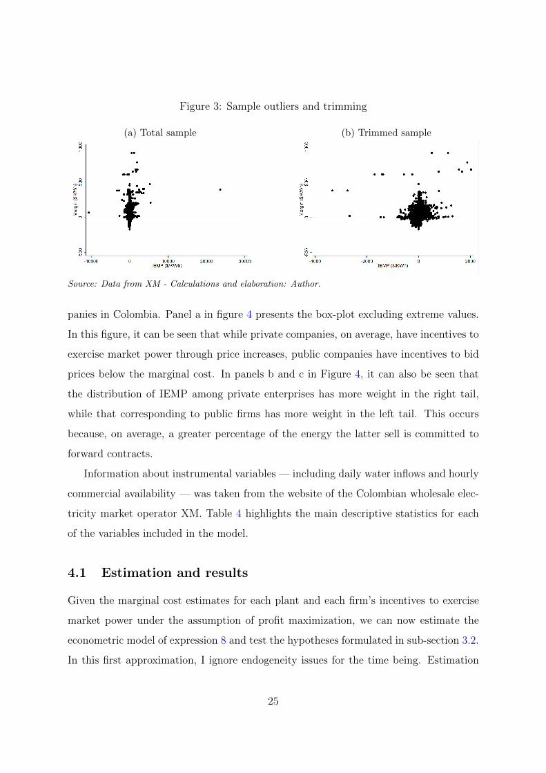
Figure 3: Sample outliers and trimming

(a) Total sample (b) Trimmed sample

Source: Data from XM - Calculations and elaboration: Author.

panies in Colombia. Panel a in figure 4 presents the box-plot excluding extreme values.

In this figure, it can be seen that while private companies, on average, have incentives to

exercise market power through price increases, public companies have incentives to bid

prices below the marginal cost. In panels b and c in Figure 4, it can also be seen that

the distribution of IEMP among private enterprises has more weight in the right tail,

while that corresponding to public firms has more weight in the left tail. This occurs

because, on average, a greater percentage of the energy the latter sell is committed to

forward contracts.

Information about instrumental variables — including daily water inflows and hourly

commercial availability — was taken from the website of the Colombian wholesale elec-

tricity market operator XM. Table 4 highlights the main descriptive statistics for each

of the variables included in the model.

4.1 Estimation and results

Given the marginal cost estimates for each plant and each firm’s incentives to exercise

market power under the assumption of profit maximization, we can now estimate the

econometric model of expression 8 and test the hypotheses formulated in sub-section 3.2.

In this first approximation, I ignore endogeneity issues for the time being. Estimation

25

Figure 4: IEMP of private and public firms

(a) Box-plot

(b) Histogram Private (c) Histogram Public

Source: Data from XM - Calculations and elaboration: Author.

of the two-way fixed e↵ects model proposed in expression 8 was performed by ordinary

least squares (OLS). Table 5 presents the results of the estimations. The specifications

presented in columns (1), (2), and (3) include monthly fixed e↵ects and generation unit

fixed e↵ects.

In the case of H1, the results in table 5 suggest that there are marked di↵erences

between private and public firms in their respective exercise of unilateral market power.

26

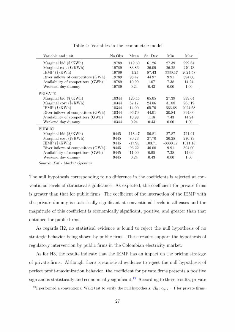
Table 4: Variables in the econometric model

Variable and unit No.Obs. Mean St. Dev. Min Max

Marginal bid ($/KWh) 19789 119.50 61.26 27.39 999.64Marginal cost ($/KWh) 19789 83.86 26.09 26.28 270.73IEMP ($/KWh) 19789 -1.25 87.43 -3330.17 2024.58River inflows of competitors (GWh) 19789 96.47 44.97 9.91 394.00Availability of competitors (GWh) 19789 10.99 1.07 7.38 14.24Weekend day dummy 19789 0.24 0.43 0.00 1.00

PRIVATEMarginal bid ($/KWh) 10344 120.45 65.05 27.39 999.64Marginal cost ($/KWh) 10344 87.17 24.06 31.88 265.19IEMP ($/KWh) 10344 14.00 65.70 -663.68 2024.58River inflows of competitors (GWh) 10344 96.70 44.01 20.84 394.00Availability of competitors (GWh) 10344 10.98 1.18 7.43 14.24Weekend day dummy 10344 0.24 0.43 0.00 1.00

PUBLICMarginal bid ($/KWh) 9445 118.47 56.81 27.87 721.91Marginal cost ($/KWh) 9445 80.23 27.70 26.28 270.73IEMP ($/KWh) 9445 -17.95 103.71 -3330.17 1311.18River inflows of competitors (GWh) 9445 96.22 46.00 9.91 394.00Availability of competitors (GWh) 9445 11.00 0.95 7.38 14.00Weekend day dummy 9445 0.24 0.43 0.00 1.00

Source: XM - Market Operator

The null hypothesis corresponding to no di↵erence in the coe�cients is rejected at con-

ventional levels of statistical significance. As expected, the coe�cient for private firms

is greater than that for public firms. The coe�cient of the interaction of the IEMP with

the private dummy is statistically significant at conventional levels in all cases and the

magnitude of this coe�cient is economically significant, positive, and greater than that

obtained for public firms.

As regards H2, no statistical evidence is found to reject the null hypothesis of no

strategic behavior being shown by public firms. These results support the hypothesis of

regulatory intervention by public firms in the Colombian electricity market.

As for H3, the results indicate that the IEMP has an impact on the pricing strategy

of private firms. Although there is statistical evidence to reject the null hypothesis of

perfect profit-maximization behavior, the coe�cient for private firms presents a positive

sign and is statistically and economically significant.19 According to these results, private

19I performed a conventional Wald test to verify the null hypothesis: H0 : ↵pri = 1 for private firms.

27

Table 5: OLS regression results

(1) (2) (3) (4)

Private IEMP 0.27*** 0.24*** 0.20*** 0.19***(0.08) (0.06) (0.06) (0.06)

Public IEMP 0.01 0.00 -0.04 -0.03(0.04) (0.03) (0.03) (0.03)

Marginal Cost 1.29*** -0.84** 0.83*** -0.26(0.19) (0.39) (0.26) (0.21)

Monthly F.E. N Y N YUnit F.E. N N Y Y

N. Obs 19789 19789 19789 19789N. Clusters 32 32 32 32R-squared 0.74 0.37 0.63 0.69Joint-Sig. 30.60*** 36.65*** 115.0*** 32.38***

Test No Di↵ 8.33 12.47 11.97 12.96p-Value 0.01 0.00 0.00 0.00Test PMP 84.17 174.14 162.37 190.25p-Value 0.00 0.00 0.00 0.00

Note: Statistical significance at standard levels (*** at 1%, ** at 5%

and * at 10%). SE clustered by unit in parentheses. Test No Di↵:

H0 : ↵pri � ↵soe = 0 and Test PMP(Profit maximization

by private firms): H0 : ↵pri = 1.

firms exercise between 19.3% and 25% of the market power predicted by theory.

In order to test the coherence of the results presented in table 5 as regards firm

heterogeneity, independent regressions of the bid price on IEMP by firm were performed

in line with McRae and Wolak (2009). Expression 8 was then estimated for the main

private and public firms. The firms analyzed account for more than 80% of the energy

generated, and in 89% of hourly periods, these same firms set the spot price. The results

of these econometric estimations are summarized in table 6 for private firms and table 7

for public firms.

Table 6 shows that the coe�cients for private firms are positive and statistically

significant. Even though they di↵er for each private firm, the coe�cient of the pooled

regression falls within the confidence intervals of the regressions for each private firm.

28

Table 6: OLS independent regressions by firm - Private

ENDESA COLINV EPSA

(1) (2) (3)

Private IEMP 0.18*** 0.20** 0.19**(0.06) (0.09) (0.09)

Marginal Cost 2.00*** -1.95 5.90***(0.44) (1.41) (1.59)

Monthly F.E. Y Y YUnit F.E. Y Y Y

N.Obs 2,485 1,531 112N. Clusters 7 6 -R-squared 0.38 0.12 0.26Joint-Sig. 8.839*** 2.452*** 6.818***

Note: Statistical significance at standard levels (*** at 1%, ** at 5%

and * at 10%). SE clustered by unit in parentheses.

Table 7: OLS independent regressions by firm - Public

ISAGEN EPM GECELCA GENSA

(1) (2) (3) (4)

Public IEMP -0.03* -0.02 -0.17*** -0.02(0.02) (0.02) (0.05) (0.02)

Marginal Cost -0.87 -0.34 -1.67*** 0.56***(0.78) (1.08) (0.61) (0.16)

Monthly F.E. Y Y Y YUnit F.E. Y Y Y Y

N.Obs 1,133 471 3,000 3,634N. Clusters - - 6 4R-squared 0.04 0.00 0.22 0.02Joint-Sig. 2.174 0.455 41.49*** 14.07**

Note: Statistical significance at standard levels (*** at 1%, ** at 5%

and * at 10%). SE clustered by unit in parentheses.

In contrast, according to table 7, the coe�cients for public firms are not statistically

significant and are even negative. These results support the hypotheses of behavioral

di↵erences between public and private firms and perfect regulatory intervention by public

29

firms.

Sub-section 3.2 sounded a warning about potential problems of endogeneity arising

from the interaction of firms and the measurement error of the IEMP. In terms of the

elements presented in expression 8, this entails relaxing the assumption that "it is un-

correlated with the IEMP. Hence, the OLS estimates must be interpreted with caution

given this potential identification problem.

As stated, to address the issue of endogeneity of the IEMP, I used instrumental

variable techniques. I performed a two-stage generalized method of moments (GMM2S)

in order to estimate the two-way fixed e↵ects proposed in expression 8. As instruments

I used the contemporary values, the quadratic transformation, and the first three lags of

the variables described in sub-section 3.2, i.e., the inflows of the rivers feeding the rival

firms’ reservoirs, the competitors’ commercial availability, and the weekend day dummy

variable.

There are two endogenous variables: the interactions Dpri

j\IEMPih and D

pub

j\IEMPih.

In the two-way fixed e↵ects model, The first stage equation for these variables is:

Downer

i⇥ \IEMPit = �0 +

2X

k=1

⇣�k

1(zk

�it)2 + �

k

2

�D

pub

i⇥ (zk

�it)2�⌘

+3X

⌧=0

2X

k=1

⇣�k

1zk

�i(t�⌧) + �k

2

�D

pub

i⇥ z

k

�i(t�⌧)

�⌘+ ✓(ccijt) + weekday + µj + 't + ⌘it

where the owner can be either private (pri) or public (pub), z1�it

is the sum of inflows

of the rivers which feed the reservoirs of the major hydroelectric units of the competitors

of agent i on day t measured in GWh, z2�it

is the sum of the commercial availability of

the competitors of agent i on day t measured in GWh, ⌧ is the lag of the variables used

as instruments, weekday is the weekend day dummy, µj represents unit fixed e↵ects, and

't are monthly fixed e↵ects. The results of these GMM2S estimations are shown in table

8. 20

20Note that column 5 of table 8 presents a specification which is a more rigorous structural interpreta-tion of profit-maximization restricted to one bid per day from each unit. If the marginal cost and IEMP

30

Table 8: Two way fixed e↵ects - GMM - results

(1) (2) (3) (4)

Private IEMP 0.67*** 0.88*** 0.89*** 0.69***(0.23) (0.19) (0.11) (0.08)

Public IEMP -0.15* -0.37** 0.04 0.27**(0.08) (0.16) (0.08) (0.11)

Marginal Cost 1.22*** -0.98*** 0.59*** -0.24***(0.05) (0.10) (0.07) (0.06)

Monthly F.E. N Y N YUnit F.E. N N Y Y

N. Obs 14836 14836 14836 14836N. Clusters 32 32 32 32Joint Sig. 360.9*** 54.26*** 112.8*** 54.83***

Weak IdentificationF first stage Private 8.83 119.00 1729.29 618.54F first stage Public 18.02 51.90 7.06 25.73K-P rk Wald F 18.81 6.83 21.83 2.45Cragg-Donald Wald F 8.9 11.13 6.93 6.23

OveridentificationHansen J 24.76 13.63 21.72 21.11p-Value 0.17 0.81 0.3 0.33

Test No Di↵ 9.31 22.06 26.27 6.62p-Value 0.00 0.00 0.00 0.00Test PMP 2.03 0.40 0.93 14.48p-Value 0.15 0.53 0.34 0.02

Note: Statistical significance at standard levels (*** at 1%, ** at 5% and * at 10%).

SE clustered by unit in parentheses. Test No Di↵:H0 : ↵pri � ↵soe = 0 and Test PMP

(Profit maximization by private firms): H0 : ↵pri = 1. The test statistics for weak

identification are the Kleibergen-Paap rk Wald F and the Cragg-Donald Wald F. H0:

Instruments are weak. The critical values for two endogenous variables and twenty-one

excluded instruments are 20.53, 11.04, and 6.10 for 5%, 10% and 20% maximal IV

relative bias, respectively, according to Stock and Yogo (2002)

In the case of H1, the GMM2S estimations yield qualitatively similar results to those

components are measured correctly, under a structural interpretation of the profit-maximization model,the empirical analog of the first-order condition should not include the constant and fixed e↵ects thatdo not appear in equation 2. As mentioned above, the fixed e↵ects would allow public firms violate themarginal cost pricing rule. The orthogonality conditions of this rigorous specification can be expressedas:

31

obtained by the OLS regressions. The null hypothesis to the e↵ect that there is no

di↵erence in the coe�cients of private and public firms is rejected. The coe�cients

of private firms are positive, statistically significant, and greater than those of public

companies.

As for H2, di↵erent results are obtained depending on the particular model specifica-

tion. For the model that ignores individual heterogeneity, the sign of the coe�cient for

public firms is negative and statistically significant. Conversely, the model that accounts

for time and unit fixed e↵ects yields a positive coe�cient that is both economically and

statistically significant.

However, it should be noted that these estimates di↵er quantitatively from those

obtained by OLS. The coe�cients from the GMM2S estimation yield values of a higher

order of magnitude, especially for private firms. These results are consistent with the

attenuation bias problem in the OLS estimators. Indeed, I found values that were three

to five times higher than those obtained when using the OLS estimation. In addition,

the value of these coe�cients is closer to the expected theoretical value of the profit-

maximization models for private firms.

As for H3, note that the specifications including time or unit fixed e↵ects do not

allow rejection of the null hypothesis at any standard level of significance. In the case

of the two-way fixed e↵ects model, the hypothesis of profit-maximization behavior by

private firms cannot be rejected at the 1% significance level.

When testing the adequacy of the instruments, the J-Hansen statistic suggests that

E⇥Z

0

ijt"it

⇤= E

hZ

0

ijt

⇥P

⇤

ijt � ✓(bcijt)� ↵pri(Dpri

j· \IEMPijt)� ↵pub(D

pub

j· \IEMPijt)

⇤i= 0

Alternatively, in column 5 of table C12 in appendix C, I present the results of a model in which Iuse the margin as the dependent variable. This entails dropping the estimation of ✓ and assuming it isequal to 1, so the orthogonality conditions can be written as:

E⇥Z

0

ijt"it

⇤= E

hZ

0

ijt

⇥(P ⇤

ijt � bcijt)| {z }Margin

� ↵pri(Dpri

j· \IEMPijt)� ↵pub(D

pub

j· \IEMPijt)

⇤i= 0

32

the models satisfy the exclusion restriction. As for the potential weakness of the instru-

ments, the F-statistic for each of the endogenous regressors meets the rule-of- thumb

threshold of values higher than 10 for the models in columns (3) and (4). Moreover,

the Cragg-Donald Wald F-statistic suggests that the GMM2S estimations presented in

table 8 have a maximum bias, which would not be more than 10% of the bias of the

OLS estimations for the models in columns (2) and not more than 20% for the models

in columns (3) and (4), according to the criteria described by Stock and Yogo (2002).

Alternatively, the Kleibergen-Paap rk Wald F-statistic suggests that the GMM2S esti-

mations presented in table 8 have a maximum bias, which would not be more than 5%

of the bias of the OLS estimations for the model in column (3), 20% for the model in

column (2) and more than 30% for the model presented in column (4), according to the

same criteria (Stock and Yogo, 2002). Although several of the models presented satisfy

some of the criteria for ruling out instrument weakness as a relevant issue, the results

presented in Table 8 should be interpreted with caution given that there is no clear

consensus regarding the criteria for detecting weak instruments when the conditional

homoskedasticity assumption is not valid.

In short, the results of the econometric exercises performed here suggest that pri-

vate firms in the Colombian wholesale electricity market are more responsive to their

incentives to exercise market power than are public firms. Moreover, there is empiri-

cal evidence in support of the hypothesis of regulatory intervention by the latter in the

Colombian electricity market. The introduction of structural elements in the identifica-

tion strategy reveals indications of attenuation bias in the OLS estimators and partial

evidence of profit-maximization behavior on the part of private firms in the Colom-

bian spot market. Overall, this indicates that the private ownership share of electricity

generation is not neutral as regards competition.

4.2 Robustness checks

The results presented above are dependent on particular specification decisions: (i) The

left hand side variable; (ii) the sample of units selected for the estimate and; (iii) the

33

choices of di↵erent parameters in the empirical implementation. Here, several estimations

of the econometric model are run to test di↵erent specifications of these alternatives.

Overall, the qualitative results of the model seem to be relatively robust to the di↵erent

options.

(i) Specification of the hand side variable The marginal price of each generator

is chosen as the left-hand side variable of the baseline econometric model. The ad-

vantage of so doing is that it is possible to obtain a coe�cient for the marginal cost

and to determine if its value and sign are consistent with expression (2). However,

it is equally possible to employ the firm’s margin as the left-hand side variable.

Thus, the margin mit = P⇤

ijt� bcijt was calculated and used as the independent

variable in the econometric model. The results are summarized in Table C12 in

appendix C. The model’s main results remain unchanged. The coe�cients of the

estimates for the private IEMP lie within the original model’s confidence interval,

while the value of the coe�cient for the SOEs is not statistically significant or is

very close to zero.

(ii) Sample of units Several concerns may arise regarding potential selection bias

in the sample used for the baseline estimation and the criterion for classifying units

as public or private.

As mentioned in section 2, around 70% of electricity in Colombia is produced from

hydroelectric resources, so it makes sense to assume that the profitability of the

most important companies in this market depends mainly on this type of resource.

Nonetheless, in the baseline estimation presented in sub-section 4.1, only observa-

tions in which the thermal units were marginal were included. This is problem-

atic because it is possible that determination of a thermal unit as marginal is not

random. This would imply that the data-generating process in circumstances in

which thermal plants are marginal is particular to those circumstances and does not

34

present a reliable general picture of the unilateral market power of private and pub-

lic firms in the Colombian wholesale electricity market, i.e., the baseline estimation

may be subject to a potential selection bias. In order to address this concern, I per-

formed a two-way fixed e↵ects estimation that also included the hydro units.21 The

results are summarized in Table C13 in appendix C. The model’s main conclusions

remain unchanged. In the two-way fixed e↵ects model (Column 4 in table C13)

the coe�cients of the OLS estimates for the private IEMP are smaller than the

baseline estimation but positive and statistically significant, while the value of the

coe�cients for the public firms is not statistically significant. Regarding the IEMP

coe�cients of the GMM estimates when hydro units are included, for both public

and private firms alike, they lie within the baseline model’s confidence intervals.

Nevertheless, these results should be interpreted with caution given the results of

the indicators of instrument weakness and also because the overidentification test

is close to the critical values for rejection of the null hypothesis.

Meanwhile, as mentioned in section 2, I classified the generation firms into “private”

and “public” according to the ownership category of the shareholder controlling the

firm that represents the unit to the market operator. However, it is possible that not

all public firms have the same incentives. In particular, there are two types of public

firm in the Colombian wholesale electricity market that might not be interested in

mitigating market power.22 In order to tackle this problem of potential incentive

misalignment and selection bias, I performed the estimation of the two way fixed

21The inclusion of this type of unit in the sample cannot be done at zero cost in relation to theassumptions necessary for the validity of the estimate. First, it must be assumed that the first-ordercondition in expression (2) is also true for both thermal and hydraulic units, excluding potential dynamiccomponents for the latter. Second, it must be assumed that the marginal cost of thermal units and theopportunity cost of water in hydraulic units are adequately modeled by unit and time fixed e↵ects.

This robustness check is inspired in the suggestion of an anonymous referee.22First, the firm EPM is the property of the municipality of Medellın. It is possible that despite being

a public company, EPM could exercise unilateral market power in the national electricity market in orderto extract additional profits from other regions and transfer these benefits to the citizens of Medellın.Second, some of the thermal units represented in the market by public firms are actually owned byprivate companies that have signed power purchase agreements (PPA) with these public firms. Thistype of public company may have di↵erent bid price incentives depending on whether the unit beingo↵ered is subject to a PPA or not. I owe this observation to an anonymous referee.

35

e↵ects model presented in section 4.1 excluding from the sample the units under

a PPA in force and the unit owned by EPM.23. The results for estimation of this

model are presented in table C14 in appendix C.

The most important qualitative results of the estimation remain unchanged. In the

two-way fixed e↵ects estimate, the coe�cients of the private IEMP are lower than

those in the baseline estimation, but they have the same order of magnitude and

are economically and statistically significant. In contrast, in the GMM2S two-way

fixed e↵ects estimate, the coe�cients for the IEMP of public firms are barely higher

than those in the baseline estimation. In any event, the test for no di↵erences is still

rejected at standard significance levels. It is important to note that the indicators

of model identification do not reveal evidence of instrument weakness or violation

of the exclusion restriction.

Another important aspect that must be accounted for in order to avoid selection

bias is related to the mechanism of electricity generation back-up for restricted

supply situations. Colombia’s generation supply is heavily dependent on its hy-

droelectric resources in drought periods which are exacerbated by El Nino events.

To guarantee supply during this phenomenon, Colombia has created a payment for

power availability, known as the “reliability charge”.24

In order to rule out the possibility that the results in the baseline estimation are

caused by ignoring the potential change in incentives due to the reliability charge

scheme, I performed the estimation of the two-way fixed e↵ects specification ex-

cluding from the sample the days on which the spot price rose above the scarcity

23Particularly, I excluded observations of the units Termocentro, Termovalle, Termoflores 1, Termo-barranquilla 3, Termobarranquilla 4, Tebsa, and Paipa 4.

24This mechanism works as a call option, where the product of the option is the obligation to generatea specific firm energy quantity. These obligations are assigned in a long-run multi-unit auction. Thereference price of the call option is the spot price of the wholesale electricity market and the strikeprice is the scarcity price. The latter is defined by the regulator and is a reference of the variable costof generation of the most expensive unit in the system. Note that during periods when the price risesabove the scarcity price, the reliability charge imposes the production of firm energy quantities at a fixedprice, just as unilateral forward contracts do. As a result, it may be that reliability charge incentivesdistort the IEMP in the spot market during critical El Nino events.

36

price for at least one hour.25

The weight of observations for which the spot price exceeds the scarcity price is

modest even when only thermal units are considered. For the entire sample (in-

cluding thermal and hydraulic resources), this situation occurred in 68 observations.

For the sample of thermal units, it occurred in 53 observations. The number of

observations eliminated by discarding the days on which the marginal price ex-

ceeded the scarcity price for at least one hour was 766 for the entire sample and

422 for the sub-sample of thermal units. As can be seen in Table C15 in appendix

C, the results of the check described above were robust and similar to the baseline

estimation.

(iii) Choices of di↵erent parameters In order to implement the econometric model,

it is necessary to rely on particular choices of several parameters such as:

a. The percentage by which the sample should be trimmed in order to eliminate

the IEMP outliers;

b. The lags of the instruments in the first stage of the IV estimations; and

c. The delta (�) parameter and the methodology for computing the incentives to

exercise market power.

First, in the baseline estimation, the sample was trimmed to exclude observations

corresponding to the 1% lowest values for the denominator of expression 9. Table

C16 in appendix C presents the estimations when trimming observations corre-

sponding to the 0.1% and 5% lowest values.

The OLS estimates of the coe�cient of private IEMP yield values that lie within

the 95% confidence interval of the baseline estimation. Similarly, the OLS estimates

of the coe�cient of private IEMP are not statistically significant or are very close

to zero. In the case of the GMM2S estimations, even though the coe�cients of the

25This robustness arises from the observations of an anonymous referee.

37

private IEMP show lower values for the sample trimmed to the 0.1% lowest values,

they are still statistically and economically significant. In the case of the IEMP of

public firms , the results remain unchanged.

Second, in the baseline estimation, the first three lags of the river inflows and the

commercial availability of competitors were used as instruments for the GMM2S

estimations. I repeated the estimations of this model using the first two and first

four lags in the instrumental variable specification. These estimations are reported

in Table C17 in appendix C, where it can be seen that they are similar to the

baseline estimation.

Finally, it is important to verify that the results of the estimates are relatively

insensitive to the computation methodology for the \IEMPijt. In the baseline es-

timation, a delta � parameter of 5% is set in order to take into account the price

window when calculating the slope of the inverse residual demand function. In

order to verify the robustness of the baseline results, the IEMP was calculated

again using � parameters of 10% and 25% and the estimations were repeated with

the same baseline econometric specification. The results are shown in table C18

in appendix C. Although the value of the private IEMP coe�cient seems to in-

crease with the delta parameter, these econometric regressions indicate that the

most important qualitative results of the baseline estimation remain unchanged.

In addition, one of the potential shortcomings of the methodology for computing

the residual demand slope based on only two points along the function, as the one

used for the baseline estimate, is that the estimate of the slope is highly sensitive

to idiosyncratically steep or flat sections of the residual demand.26 In order to rule

out the possibility that this weak point may distort the final results, I applied a

smoothing approach that has been implemented by several authors (Reguant, 2014;

Wolak, 2003, 2007) in the context of electricity auctions. This approach uses all

the steps of the residual demand function to compute the slope. For a given hour

26This robustness check arises from the suggestion of an anonymous referee.

38

of the day the derivative of the residual demand faced by a firm is approximated

as follows:

@DRith(s⇤ijt)

@s⇤

ijt

= �1

h

KX

k=1

q�ikt��(s⇤

ijt� s�ikt)/h

�

where s⇤

ijtis the marginal price of firm i in hour t, K is the number of genera-

tion units supplied by the rivals of firm i, q�ikt is the quantity supplied by unit

k owned by a rival in hour t and s�ikt is the bid for this unit, �(t) is the stan-

dard normal density function, and h is the smoothing parameter. I applied three

di↵erent smoothing parameters: h = 200, h = 400 and h = 800,27 and used this

calculation of the residual demand slope to compute the daily \IEMPijt, repeating

the econometric estimations. As can be seen in tables C19, C20 and C21 in ap-

pendix C the smoothing parameter methodology has a relatively minor e↵ect on

the estimates and does not invalidate the most important qualitative results of the

baseline model.

4.3 E�ciency gains from market power mitigation

An important question that arises from the hypothesis of market power mitigation be-

havior by public companies is what level of e�ciency gains is achieved due to public

companies ignoring the incentives to exercise market power? 28

In this paper, it has been assumed that the total demand for electricity is inelastic.

This implies that losses in consumer surplus are transferred to a larger producer surplus

and hence the deadweight losses arise from the supply side. In this context, it is possible

to identify two sources of potential e�ciency gains. The first consists of the rival’s

incentive e↵ect. This arises because the supply of prices with market power mitigation by

public companies implies that private companies are faced with flatter residual demand

curves. On the other hand, it is also possible to identify a merit order e↵ect. This

27I use these parameters because the standard deviation of the bids of the units participating in themarket in the study period is around 400.

28This sub-section arises from the suggestion of an anonymous referee.

39

originates from the e�ciency gains that result from the displacement of higher-cost

plants owned by private companies as a consequence of public companies bidding at

competitive prices. Despite the importance of these e↵ects, the calculation of each of

these components presents several di�culties.

Regarding the rival’s incentive e↵ect, once the counterfactual of a profit-maximizing

public company is added, then in order to perform a complete calculation of the compa-

nies’ response it would be necessary to calculate the new equilibrium under this counter-

factual. To perform this task, it may be necessary to assume an oligopolistic competition

model and a functional form for the marginal costs of the firms, an exercise that goes

beyond the scope of this paper.

In relation to the merit order e↵ect, it is necessary to have estimates of the marginal

costs in order to build the competitive supply of public and private firms and calculate

the generation costs both in equilibrium with market power mitigation and in the coun-

terfactual equilibrium in which the public company maximizes profits. As mentioned

above, there are estimates of the marginal costs of thermal units but not for hydro

plants. Therefore, there is no choice but to make some kind of assumption regarding

the marginal cost of the water units. In the context of this sub-section of the paper, it

will be assumed that all the firms bid the marginal costs of water units. This allows the

results of the calculations to be interpreted as a lower bound of the merit order e↵ect.

To calculate the merit order e↵ect, the following steps were adopted:

1. First, three counterfactual scenarios of privatization of a number of companies

owned by central government are constructed.

– In the first counterfactual scenario, it is assumed that the ISAGEN company

was privately owned from 2005 to 2015.

– In the second counterfactual scenario, it is assumed that the ISAGEN and

GECELCA companies formed a single synthetic firm and that this firm was

privately owned from 2005 to 2015.

40

– In the third counterfactual scenario, it is assumed that the companies IS-

AGEN, GECELCA, and GENSA comprise a single synthetic firm and that

this firm was privately owned from 2005 to 2015.

2. Second, the residual demand curve and the total cost curve of the synthetic com-

pany are constructed for each hour of the day. Water resources are assumed to be

being bet at the marginal cost.

3. Third, each firm’s profits are calculated as the income obtained at each point

of residual demand minus the accumulated costs at the corresponding level of

production. To calculate the profit function, two cases arise:

– The profits that the firm would obtain if it did not have energy committed in

forward contracts.

– The profits that the firm would obtain according to the forward contracts

observed in the sample.

The prices and quantities in the residual demand that maximize profits in each

scenario and case are found. The generation quantities and costs corresponding to

the optimal solution are calculated.

4. Fourth, the competitive supply curve is constructed. The bidding prices of the

thermal units are replaced by the marginal costs for the counterfactual privatized

firm. Here it is also assumed that the bidding prices of the water units reflect their

marginal cost. Subsequently, the market power mitigation equilibrium is calculated

and the generation levels and costs corresponding to this equilibrium are computed.

5. Fifth, the generation costs in each counterfactual scenario and each case of speci-

fication of the profit function (with and without contracts) are compared with the

generation costs resulting from the market power mitigation equilibrium.

41

The results of applying this methodology in scenario 1 are presented in table 9, those

corresponding to scenario 2 are presented in table 10, and those corresponding to scenario

3 are presented in table 11.

Table 9: E�ciency gains of market power mitigation: scenario 1

Millions of Colombian pesos

Year Total Cost E�ciency Loss E�ciency Loss E�ciency Loss % E�ciency Loss %MP Mitigation No Forward C. With Forward C. No Forward C. With Forward C.

2005 6515.51 97.88 5.97 1.22% 0.09%2006 6565.00 116.66 7.10 1.46% 0.12%2007 7666.48 91.00 2.92 0.97% 0.04%2008 7581.96 217.56 9.31 2.42% 0.12%2009 12535.94 91.31 9.28 0.66% 0.08%2010 12730.86 101.32 14.33 0.92% 0.18%2011 7385.82 114.14 10.28 1.57% 0.16%2012 12009.47 117.35 11.83 1.39% 0.14%2013 17456.32 124.19 7.70 0.72% 0.06%2014 20639.42 180.26 5.50 0.88% 0.03%

Table 10: E�ciency gains of market power mitigation: scenario 2

Millions of Colombian pesos

Year Total Cost E�ciency Loss E�ciency Loss E�ciency Loss % E�ciency Loss %MP Mitigation No Forward C. With Forward C. No Forward C. With Forward C.

2005 5502.50 277.36 20.99 4.00% 0.34%2006 6130.29 387.00 13.79 5.02% 0.20%2007 6722.82 336.92 12.03 4.25% 0.18%2008 6963.17 643.17 30.70 7.80% 0.36%2009 11160.04 445.72 39.85 3.49% 0.30%2010 11492.94 345.04 46.30 2.82% 0.34%2011 7041.47 271.82 16.13 3.35% 0.17%2012 11150.43 243.47 9.10 2.20% 0.08%2013 15842.11 575.75 21.48 3.40% 0.16%2014 18720.37 672.93 34.98 3.67% 0.18%

In the case in which the counterfactual company does not have energy committed in

contracts, the impact in the first scenario (ISAGEN private) varies between 0.66% and

2.42% of the cost of a non-privatization situation, an e↵ect that seems quite modest if

we consider that ISAGEN is among the three most important firms in the electricity

generation market in Colombia. The explanation for this is that the ISAGEN company

only has one thermal unit (Termocentro) and the model presented above only captures

42

Table 11: E�ciency gains of market power mitigation: scenario 3

Millions of Colombian pesos

Year Total Cost E�ciency Loss E�ciency Loss E�ciency Loss % E�ciency Loss %MP Mitigation No Forward C. With Forward C. No Forward C. With Forward C.

2005 5502.50 277.36 20.99 4.00% 0.34%2006 6147.04 492.22 14.20 6.40% 0.17%2007 6668.42 435.08 18.38 5.49% 0.23%2008 6952.99 781.66 23.66 9.53% 0.29%2009 11182.01 611.68 50.57 4.81% 0.30%2010 11567.71 455.06 56.75 3.62% 0.34%2011 7109.33 333.13 22.37 4.03% 0.21%2012 11171.03 302.33 8.91 2.61% 0.06%2013 15887.09 790.21 25.29 4.62% 0.15%2014 18609.15 846.85 77.10 4.75% 0.33%

the e↵ect of the merit order of thermal units. In the second (GECELA and ISAGEN

private) and third scenarios (GECELA, GECELCA, and GENSA private), more impor-

tant e↵ects are observed that vary between 2.82% and 7.82% for the second case and

2.61% and 9.52% for the third.

This variation seems to be explained to some extent by fluctuations in water resources

caused by El Nino and La Nina phenomena. In 2011, significantly lower generation costs

were observed, which coincided with the abundance of water resources generated by a

fairly intense La Nina phenomenon. On the other hand, higher generation costs were

observed in 2014. One explanation for this may be that November and December of this

year witnessed the start of the worst El Nino phenomenon observed in a decade.

In the case in which the counterfactual company has energy committed in forward

contracts according to the quantities observed in the sample, the e�ciency gains by the

merit order e↵ect in the three scenarios considered is negligible. In the first it varies

from 0.03% to 0.18%, in the second from 0.08% to 0.36%, and in the third from 0.06%

to 0.34%.

As in the previous case, this result can be partially explained by the fact that the

proposed methodology only captures the merit order e↵ect of thermal units. However,

the di↵erence in results between the first and second cases shows that levels of forward

contracts play a determining role in the possibilities of mitigating market power in the

43

spot electricity market.

As mentioned above, it is possible that a company that intends to mitigate market

power applies this policy in deciding its forward contractual positions, thus conditioning

how much potential market power it has in the short-term market. In the case that

considers the observed forward contracts levels, the results suggest that given the for-

ward contracting position of public firms, there are no major di↵erences between the

equilibrium that would be obtained from profit maximization and application of the

marginal cost pricing rule. This can happen because public companies have signed con-

tracts in such a way that they have little incentive to exercise market power in the spot

market. Of course, this interpretation is based on the strong assumption that the firms

used to construct the counterfactual scenario bid their water resources according to their

marginal costs.

In my opinion, given that the evidence presented in sub-section 4.3 suggests that

public companies exert market power mitigation in the short-term market, it is quite

possible that these same companies are also exerting such mitigation in the forward

contract market. This leads me to consider that the e�ciency gains from market power

mitigation behavior in the Colombian spot electricity generation market are modest.

5 Conclusions

In this study, bid price information for the Colombian electricity market has been used

to understand di↵erences in the way in which private and public firms exercise market

power. Here, the methodology developed by McRae and Wolak (2009) has been extended

to include firms that do not price strategically. A new interpretation is proposed of the

impact of incentives to exercise market power on prices in an attempt to obtain evidence

of the profit-maximizing behavior of private firms and the adoption of the marginal cost

pricing rule by public firms.

Estimations of the semi-elasticity of demand combined with contracting information

suggest that the generators analyzed — both state-owned and private — had incentives

44

to exercise market power in association with profit-maximization behavior. An econo-

metric analysis was conducted to find statistical evidence of: i) di↵erences in the impact

of incentives to exercise market power on the bids and prices of state-owned and private

firms; ii) the non-exercise of market power by public companies in accordance with the

marginal cost pricing rule; and iii) the exercise of market power by private firms con-

sistent with profit-maximization behavior. Based on the outcomes of these econometric

estimations, two main conclusions can be drawn. First, marked di↵erences exist in the

way in which private and state-owned firms exercise unilateral market power: Specifi-

cally, private generators in the Colombian market are more responsive to IEMP than

are public firms. Second, public firms exercise regulatory intervention in the Colombian

electricity markets - that is, they are not responsive to IEMP.

These findings suggest that the ownership regime of firms in Colombia’s electricity

industry is not neutral as regards the exercise of market power. Moreover, the outcomes

reported have important implications for the regulation of electricity markets and the

privatization of state-owned firms. First, besides increasing competition, there would

appear to be an alternative way to achieve e�ciency, namely, the mitigation of market

power by state-owned companies. Likewise, regulators need to recognize the nature of

ownership within the market they are designing and determine whether public companies

implement market power mitigation strategies. Second, the absence of neutrality in

the exercise of market power implies that privatization has indirect e↵ects on market

competitiveness. This means the government should take into account the possible anti-

competitive e↵ects that privatization might have and include these undesirable costs in

their assessment of the sales operation of state-owned generation units.

References

Allaz, B. and J.-L. Vila (1993). Cournot competition, forward markets and e�ciency.

Journal of Economic Theory 59 (1), 1–16.

Barros, F. and L. Modesto (1999). Portuguese banking sector: a mixed oligopoly?

45

International Journal of Industrial Organization 17 (6), 869–886.

Beato, P. and A. Mas-Colell (1984). The marginal cost pricing rule as a regulation

mechanism. in M. Marchand, P. Pestieau and H. Tulkens (eds), The Performance of

Public Enterprises, Amsterdam: North-Holland , 81–100.

Bel, G., X. Fageda, and M. E. Warner (2010). Is private production of public services

cheaper than public production? a meta-regression analysis of solid waste and water

services. Journal of Policy Analysis and Management 29 (3), 553–577.

Berry, S., J. Levinsohn, and A. Pakes (1995). Automobile prices in market equilibrium.

Econometrica 63 (4), 841–90.

Borenstein, S. and J. Bushnell (1999). An empirical analysis of the potential for market

power in california’s electricity industry. Journal of Industrial Economics 47 (3), 285–

323.

Borenstein, S., J. Bushnell, and F. A. Wolak (2002). Measuring market ine�ciencies

in california’s restructured wholesale electricity market. American Economic Re-

view 92 (5), 1376–1405.

Bos, D. (2015). Pricing and price regulation: an economic theory for public enterprises

and public utilities. Elsevier.

Bushnell, J., E. Mansur, and C. Saravia (2008). Vertical arrangements, market struc-

ture, and competition: An analysis of restructured us electricity markets. American

Economic Review 98 (1), 237–66.

Corts, K. S. (1999). Conduct parameters and the measurement of market power. Journal

of Econometrics 88 (2), 227–250.

De Fraja, G. and F. Delbono (1989). Alternative strategies of a public enterprise in

oligopoly. Oxford Economic Papers 41 (2), 302–11.

46

Fabra, N. and M. Reguant (2014). Pass-through of emissions costs in electricity markets.

American Economic Review 104 (9), 2872–99.

Fershtman, C. and K. Judd (1987). Equilibrium incentives in oligopoly. American

Economic Review 77 (5), 927–40.

Frydman, R., C. Gray, M. Hessel, and A. Rapaczynski (1999). When does privatization

work? the impact of private ownership on corporate performance in the transition

economies. The quarterly journal of economics 114 (4), 1153–1191.

Garcia, A. and L. E. Arbelaez (2002). Market power analysis for the colombian electricity

market. Energy Economics 24 (3), 217–229.

Green, R. and D. M. Newbery (1992). Competition in the british electricity spot market.

Journal of Political Economy 100 (5), 929–53.

Hortacsu, A., F. Luco, S. L. Puller, and D. Zhu (2019). Does strategic ability a↵ect

e�ciency? evidence from electricity markets. American Economic Review 109 (12),

4302–42.

Hortacsu, A. and S. Puller (2008). Understanding strategic bidding in multi-unit auc-

tions: a case study of the texas electricity spot market. RAND Journal of Eco-

nomics 39 (1), 86–114.

Kay, J. A. and D. J. Thompson (1986). Privatisation: a policy in search of a rationale.

The economic journal 96 (381), 18–32.

Klemperer, P. and M. Meyer (1989). Supply function equilibria in oligopoly under un-

certainty. Econometrica 57 (6), 1243–77.

La Porta, R. and F. Lopez-de Silanes (1999). The benefits of privatization: Evidence

from mexico. The Quarterly Journal of Economics 114 (4), 1193–1242.

Matsumura, T. (1998). Partial privatization in mixed duopoly. Journal of Public Eco-

nomics 70 (3), 473–483.

47

McRae, S. and F. A. Wolak (2009). How do firms exercise unilateral market power? evi-

dence from a bid-based wholesale electricity market. RSCAS Working Papers 2009/36,

European University Institute.

Mercadal, I. (2019). Dynamic competition and arbitrage in electricity markets: The role

of financial traders. Available at SSRN 3281886.

Netter, J. M. and W. L. Megginson (2001). From state to market: A survey of empirical

studies on privatization. Journal of Economic Literature 39 (2), 321–389.

Puller, S. L. (2009). Estimation of competitive conduct when firms are e�ciently col-

luding: addressing the corts critique. Applied Economics Letters 16 (15), 1497–1500.

Reguant, M. (2014). Complementary bidding mechanisms and startup costs in electricity

markets. Review of Economic Studies 81 (4), 1708–1742.

Seim, K. and J. Waldfogel (2013). Public monopoly and economic e�ciency: Evidence

from the pennsylvania liquor control board’s entry decisions. American Economic

Review 103 (2), 831–62.

Stock, J. and M. Yogo (2002). Testing for weak instruments in linear iv regression.

NBER Technical Working Papers 0284, National Bureau of Economic Research, Inc.

Sweeting, A. (2007). Market power in the england and wales wholesale electricity market

1995–2000. The Economic Journal 117 (520), 654–685.

Wolak, F. (2000). An empirical analysis of the impact of hedge contracts on bidding

behavior in a competitive electricity market. International Economic Journal 14 (2),

1–39.

Wolak, F. A. (2003). Measuring unilateral market power in wholesale electricity markets:

The california market, 1998 – 2000. American Economic Review 93 (2), 425–430.

Wolak, F. A. (2007). Quantifying the supply-side benefits from forward contracting in

wholesale electricity markets. Journal of Applied Econometrics 22 (7), 1179–1209.

48

Wolfram, C. D. (1998). Strategic bidding in a multiunit auction: An empirical analysis

of bids to supply electricity in england and wales. RAND Journal of Economics 29 (4),

703–725.

Wolfram, C. D. (1999). Measuring duopoly power in the british electricity spot market.

American Economic Review 89 (4), 805–826.

49

Appendix A Derivation of the daily version of the

IEMP

The problem the generator faces is that of designing a set of daily bids Sit = {si1t, si2t, · · · , sijt,

· · · , siNt}, where sijt is the daily bid price on day t for the energy of unit j, owned by

firm i and N is the number of units that this firm i is able to bid. These bids are ordered

from lowest to highest, so that they maximize the expected daily profit ⇡it, which is the

sum of the hourly profits ⇡ith. If we adopt a residual demand approach, in which the

competitors’ bids are given, the generator should choose the bids that clear the market

in the 24 hours of day t, constrained by the capacity of its own units and the market

clearing price rules. Let ⇡it(Sit) be the daily profits of firm i on day t ; let DRith be the

residual demand of firm i on day t at hour h; and, let Sit be the set of bids made by firm

i during day t. When considering forward contracts, the profit maximization problem of

the firm can be stated as:

maxSit

⇡it(Sit) = maxSit

"24X

h=1

⇣pth

�DRith(Sit)

��DRith(Sit)� q

c

ith

�⌘

+24X

h=1

pc

ithqc

ith�

24X

h=1

Cit

�DRith(Sit)

�#

Subject to capacity constraints and non-negativity conditions:29

0 qjith qji

If the restrictions are not binding,30 the first order conditions of this problem are:

29In the equilibrium the residual demand of firm i is equal to the total production of electricity offirm i, DRith(sjith) =

Pmj=1 qjith, where the units 1 to m are the units that produce electricity, i.e., the

units 1 to m have bids lower or equal to the marginal price and the units (m+1) to N have bids higherthan the marginal cost, hence, the former are called to produce electricity while the latter not. That isthe way by which qijth is implicitly included in the objective function.

30Note that I am interested in the units that are marginal (the equilibrium bid of the firm). We haveto assume that around the equilibrium there are not capacity constraints. This is not reasonable whenthe marginal unit is the most expensive and it is operating at full capacity. An empirical indicator of

50

24X

h=1

"@pth

@sijt

�DRith(Sit)� q

c

ith

�#+

24X

h=1

pth

�DRith(Sit)

�@DRith(Sit)

@sijt

�

24X

h=1

@Cit

�DRith(Sit)

�

@DRith

@DRith(Sit)

@sijt= 0

Given the residual demand approach and the market clearing price rule, the equi-

librium price of the market (or marginal price) is pth = min(si1t, si2t, · · · , sijt, · · · , siNt)

(the index j orders the units owned by firm i from the cheaper to the most expensive),

such that:

DRith(simt) =mX

j=1

qijt

where the marginal unit is the m-th most expensive unit owned by firm i. Once

the units of firm i are ordered by merit, the above condition means that the spot price

is equal to the bid of the generator’s marginal unit, pth = simt, if plant m clears the

market in hour h. This in turn implies that @pth

@simt

= 1. In addition, in line with previous

studies in the literature (Reguant, 2014), I assume that the residual demand of hour t

is a function of the bid of unit m that is marginal in this hour h, but not of the bids of

the other units. This implies that the derivative of the residual demand of hour h with

respect to the bids of the plants that are not marginal in that hour is equal to zero, i.e

@DRith(simt)@sijt

= 0 where m 6= j and that the derivative of the price of hour h with respect

to the bids of the plants that are not marginal in that hour is equal to zero i.e., @pth

@sijt= 0,

if unit j is not marginal.

Note that the set of potential bids that the generator is able to bet is limited by

the daily bid constraint. If the day has 24 periods with di↵erent residual demands, the

generator owns N units, and N < 24, then in at least 24 � N periods the generator

this is the percentage of observations in which the firms are operating at full capacity. In the sampleconsidering only marginal thermal units, in about 3.5% of the observations the firm is operating at fullcapacity. After repeating the econometric estimations excluding these observations from the sample,the basic results of the baseline estimation hold.

51

will not be able to choose the exact bid that clears the market in the profit-maximizing

point of each hour. In fact, the generator is compelled to clear the market with the bid

of one unit, let simt, for several hours of the day. Hence, if unit m is marginal in hours

h and h+k, this means that pth = pt(h+k). In this way, every hour can be linked to a

marginal plant m. Considering all of the above, if Hijt is defined as the set of hours of

day t where unit j is marginal (and unit j is owned by firm i), the first order condition

can be expressed as:

X

h2Hijt

(DRith(sijt)� qc

ith) + sijt

X

h2Hijt

@DRith(sijt)

@sijt�

X

h2Hijt

@Cit

@DRith

@DRith(sijt)

@sijt= 0

The optimal bids for unit j s⇤

ijtfor a private firm should be such that:

s⇤

ijt=

Ph2Hijt

@Cit

@DRith

@DRith(sijt)@sijt

�P

h2Hijt(DRith(sijt)� q

c

ith)

Ph2Hijt

@DRith(sijt)@sijt

If we assume the marginal cost of unit j to be constant during day t, the optimal bid

of a daily profit-maximizing firm can be expressed s⇤

ijtas:

s⇤

ijt= cijt +

�P

h2Hijt(DRith(sijt)� q

c

ith)

Ph2Hijt

@DRith(sijt)@sijt

Appendix B Details of the marginal cost calculus for

thermal units

The marginal costs of thermal plants were computed based on the heat rate, fuel costs,

and fuel transportation costs according to the following formula:

Exchange R.t| {z }COP$US$

⇥⇥Heat R.i| {z }

MBTU

KWh

⇥ (Transp. fuel costi + Fuel costt)| {z }US$

MBTU

⇤= Marginal Costit| {z }

COP$kWh

52

Where COP are Colombian pesos, MBTU are one thousand British thermal unit,

US are United States dollars, and KWh is one kilowatt per hour. The heat rate is a

measure of the thermal e�ciency of the generation unit. It represents the quantity of fuel

measured in MBTU necessary to generate one kilowatt per hour. The parameters of the

heat rate of thermal electricity generation units were extracted from reports published

the Mines and Energy Planning Unit (UPME).

In the case of gas-fired units, the fuel cost is based on the price of gas from the Guajira

Basin, which is the most important gas supply source for Colombian thermal generation.

From September 1995 to August 2013, the Colombian Government regulated the price of

gas obtained from this source by imposing a maximum sale price for gas. This maximum

price at period t, pt, is given by the formula pt�1[indext�1/indext�2] where indext�1 is

the average of the last semester of the New York Harbor Residual Fuel Oil 1.0 % Sulfur

LP Spot Price according to the series that was published by the US Energy Information

Administration. A period t is defined as a semester and it changes on the 1st February

and 1st August of each year.31 This price is given in US dollars/MBTU.

From 2005 to 2013, I applied the Guajira regulated price calculation published by

the most important gas producer in the market (ECOPETROL) and converted the

resulting price (US dollars/MBTU) to Colombian pesos/KWh. The exchange rate data

was obtained from the Colombian Central Bank (Banco de la Republica). For the years

after 2013, the weighted average gas price was calculated according to type of contract,

based on information about wholesale gas transactions listed on the web page of the Gas

Market Operator in Colombia (BEC).

Consequently, for gas-fired units, transportation costs were calculated as the sum of

the fees for use of each segment of the gas transmission network necessary to transport

the gas from the Guajira well to the respective generation units. These fees are regulated

by the CREG and are published in regulatory acts (CREG 70 and 125 of 2003).

As regards coal-fired units, given that Colombia is a net exporter of coal, I used

the FOB export price of thermal coal available in the Colombian Mines and Energy

31The formula was established in Act 119/2005 of CREG.

53

Planning Unit (UPME) databases. The price in dollars per ton was converted into

dollars per MBTU units, multiplying by a calorific value of Colombian thermal coal

of 1,370 btu per pound (source: regulation 2009 180507 Colombian Ministry of Energy

and Mines). To compute coal transportation costs, I used an import parity approach.

According to this criterion, transportation costs are estimated as the fee in COP per ton

for road freight transportation from the closest importation port to the location of the

generation unit. These fees were extracted from information provided by the Columbian

Ministry of Transport on e�cient road freight transportation costs.

54

Appen

dix

CRobustnessCheckTables

Tab

leC12:Estim

ationusingmarginas

dep

endentvariab

le

OLS

GMM2S

(1)

(2)

(3)

(4)

(5)

(6)

(7)

(8)

Priva

teIE

MP

0.35***

0.23***

0.19***

0.18***

1.79***

0.99***

0.77***

0.72***

(0.08)

(0.07)

(0.06)

(0.06)

(0.19)

(0.20)

(0.07)

(0.06)

PublicIE

MP

-0.04

0.03

-0.04

-0.03

-1.92***

-0.56***

-0.16**

0.31***

(0.02)

(0.04)

(0.03)

(0.03)

(0.33)

(0.17)

(0.06)

(0.08)

Mon

thly

F.E

.NO

YES

NO

YES

NO

YES

NO

YES

Unit

F.E

.NO

NO

YES

YES

NO

NO

YES

YES

N.Obs

1978

919

789

1978

919

789

1483

614

836

1483

614

836

N.Clusters

3232

3232

3232

3232

JointSig.

10.9***

7.643***

119.1**

*4.760***

60.10***

12.31***

66.55**

*70.42***

Wea

kIden

tifica

tion

FfirststagePriva

te13

.51

113

.99

57665

.97

678.9

FfirststagePublic

19.84

124.46

3.1

42.27

K-P

rkW

ald

F13.60

6.285

2.903

2.505

Cragg-D

onald

Wald

F24.61

10.66

6.748

5.874

Ove

riden

tifica

tion

Han

senJ

28.30

23.27

18.04

19.97

p-V

alue

0.0778

0.226

0.52

00.397

TestNoDi↵

21.79

7.35

11.04

11.64

94.85

21.83

112.60

17.95

p-V

alue

0.00

0.00

0.00

0.00

0.00

0.00

0.00

0.00

TestPMP

67.32

138.21

162.98

197.00

17.66

0.00

10.33

19.64

p-V

alue

0.00

0.01

0.00

0.00

0.00

0.96

0.00

0.00

Note:Statisticalsignifica

nce

atstandardleve

ls(***at1%,**at5%

and*at10%).

SE

clustered

byunit

inparenth

eses.

TestNoDi↵:H

0:↵pri�

↵soe=

0andTestPMP

(Profitmaxim

izationbypriva

tefirm

s):H

0:↵pri=

1.

Thetest

statisticsforwea

kiden

tifica

tionare

theKleibergen

-Paaprk

Wald

Fandth

eCragg-D

onald

Wald

F.H0:Instru

men

tsare

wea

k.Thecriticalva

lues

fortw

oen

doge

nou

sva

riab

lesandtw

enty

oneex

cluded

instru

men

tsare

20.53,11.04and

6.10for5%,10%,and20%

maxim

alIV

relativebias,

resp

ective

ly,accord

ingto

Stock

andYogo(2002).

55

Tab

leC13:Estim

ationincludinghy

dro

units

OLS

GMM2S

(1)

(2)

(3)

(4)

(5)

(6)

(7)

(8)

Priva

teIE

MP

0.44***

0.13**

0.12**

0.10**

4.91***

0.45***

0.62*

**

0.72**

*(0.09)

(0.05)

(0.05)

(0.04)

(0.27)

(0.12)

(0.20)

(0.11)

PublicIE

MP

0.01

-0.00

-0.04***

-0.02

3.72***

0.60***

-2.18***

0.17

(0.04)

(0.02)

(0.01)

(0.01)

(0.29)

(0.16)

(0.41)

(0.13)

Mon

thly

F.E

.NO

YES

NO

YES

NO

YES

NO

YES

Unit

F.E

.NO

NO

YES

YES

NO

NO

YES

YES

N.Obs

52,154

52,154

52,154

52,154

4054

440

,544

40,544

40,544

N.Clusters

5353

5353

5353

5353

JointSig.

12.48***

3.194**

7.310**

3.341**

276.7***

9.652***

21.12***

30.21***

Wea

kIden

tifica

tion

FfirststagePriva

te4.90

13.69

7.67

5.96

FfirststagePublic

4.80

14.68

1.13

2.26

K-P

rkW

ald

F4.79

9.43

1.13

2.17

Cragg-D

onald

Wald

F48.89

42.99

4.29

3.65

Ove

riden

tifica

tion

Han

senJ

31.82

33.47

30.70

31.92

p-V

alue

0.03

0.02

0.04

0.03

TestNoDi↵

19.35

6.16

9.73

6.62

7.77

0.80

42.07

7.21

p-V

alue

0.00

0.01

0.00

0.01

0.01

0.37

0.06

0.01

TestPMP

40.03

308.48

328.00

415.38

205.99

19.08

3.49

6.15

p-V

alue

0.00

0.00

0.00

0.00

0.00

0.00

0.00

0.01

Note:Statisticalsignifica

nce

atstandardleve

ls(***at1%,**at5%

and*at10%).

SE

clustered

byunit

inparenth

eses.

TestNoDi↵:H

0:↵pri�

↵soe=

0andTestPMP

(Profitmaxim

izationbypriva

tefirm

s):H

0:↵pri=

1.

Thetest

statisticsforwea

kiden

tifica

tionare

theKleibergen

-Paaprk

Wald

Fandth

eCragg-D

onald

Wald

F.H0:Instru

men

tsare

wea

k.Thecriticalva

lues

fortw

oen

doge

nou

sva

riab

lesandtw

enty

oneex

cluded

instru

men

tsare

20.53,11.04,and

6.10for5%,10%,and20%

maxim

alIV

relativebias,

resp

ective

ly,accord

ingto

Stock

andYogo(2002).

56

Tab

leC14:Estim

ationExcludingEPM

andPPA

OLS

GMM2S

(1)

(2)

(3)

(4)

(5)

(6)

(7)

(8)

Priva

teIE

MP

0.29***

0.21***

0.16***

0.16***

0.93***

0.74***

0.22

0.52***

(0.05)

(0.05)

(0.05)

(0.06)

(0.32)

(0.21)

(0.21)

(0.02)

PublicIE

MP

0.00

0.01

-0.02

-0.02**

0.09

-0.28

0.06

0.36*

**

(0.03)

(0.04)

(0.02)

(0.01)

(0.40)

(0.19)

(0.10)

(0.03)

Marginal

Cost

1.22

***

-0.83*

**0.64

***

-0.33*

*1.17

***

-0.76*

**0.55

***

-0.32*

**(0.08)

(0.23)

(0.11)

(0.15)

(0.08)

(0.20)

(0.11)

(0.02)

Mon

thly

F.E

.NO

YES

NO

YES

NO

YES

NO

YES

Unit

F.E

.NO

NO

YES

YES

NO

NO

YES

YES

N.Obs

1588

814

984

1498

414

984

1199

111

344

1134

411

344

N.Clusters

206

190

190

2518

817

217

225

JointSig.

117.7***

10.17***

14.40*

**

5.932***

191.8***

8.399***

12.47*

**

2462***

Wea

kIden

tifica

tion

FfirststagePriva

te3.57

6.66

1.23

97.94

FfirststagePublic

2.32

3.84

1.68

901.35

K-P

rkW

ald

F2.72

2.78

1.13

78.82

Cragg-D

onald

Wald

F12.20

14.96

1.08

2.75

Ove

riden

tifica

tion

Han

senJ

44.25

33.27

37.21

20.30

p-V

alue

0.00

0.02

0.01

0.38

TestNoDi↵

21.46

8.52

10.50

8.59

2.06

10.83

0.48

11.83

p-V

alue

0.00

0.00

0.00

0.00

0.15

0.00

0.00

0.00

TestPMP

196

.10

210.52

269.93

189.43

0.05

1.51

13.24

530.13

p-V

alue

0.00

0.00

0.00

0.00

0.82

0.22

0.49

0.00

Note:Statisticalsignifica

nce

atstandardleve

ls(***at1%,**at5%

and*at10%).

SE

clustered

byunit

inparenth

eses.

TestNoDi↵:H

0:↵pri�

↵soe=

0andTestPMP

(Profitmaxim

izationbypriva

tefirm

s):H

0:↵pri=

1.

Thetest

statisticsforwea

kiden

tifica

tionare

theKleibergen

-Paaprk

Wald

Fandth

eCragg-D

onald

Wald

F.H0:Instru

men

tsare

wea

k.Thecriticalva

lues

fortw

oen

doge

nou

sva

riab

lesandtw

enty

oneex

cluded

instru

men

tsare

20.53,11.04,and

6.10for5%,10%,and20%

maxim

alIV

relativebias,

resp

ective

ly,accord

ingto

Stock

andYogo(2002).

57

Tab

leC15:Estim

ationexcludingob

servationsduringreliab

ilitycharge

OLS

GMM2S

(1)

(2)

(3)

(4)

(5)

(6)

(7)

(8)

Priva

teIE

MP

0.17*

*0.11**

0.06**

0.06**

0.79***

0.98***

0.78***

0.66***

(0.08)

(0.04)

(0.03)

(0.02)

(0.24)

(0.20)

(0.14)

(0.07)

PublicIE

MP

0.07

0.06*

0.01

0.01

-0.21**

-0.27

0.07

0.29**

(0.05)

(0.03)

(0.02)

(0.01)

(0.09)

(0.21)

(0.06)

(0.11)

Marginal

Cost

1.29

***

-0.81*

0.81

***

-0.25

1.17

***

-0.92*

**0.64

***

-0.23*

**(0.19)

(0.40)

(0.26)

(0.20)

(0.04)

(0.11)

(0.08)

(0.07)

Mon

thly

F.E

.NO

YES

NO

YES

NO

YES

NO

YES

Unit

F.E

.NO

NO

YES

YES

NO

NO

YES

YES

N.Obs

1945

019

450

1945

019

450

1463

614

636

1463

614

636

N.Clusters

3232

3232

3232

3232

JointSig.

24.86***

10.42***

4.842*

**

2.643*

473.0***

45.30***

102.5***

55.81***

Wea

kIden

tifica

tion

FfirststagePriva

te6.97

54.54

1776.35

365

.17

FfirststagePublic

9.8

40.26

12

17.98

K-P

rkW

ald

F10.92

5.50

7.56

3.51

Cragg-D

onald

Wald

F8.61

10.87

6.82

5.92

Ove

riden

tifica

tion

Han

senJ

26.18

13.30

20.15

21.65

p-V

alue

0.12

50.823

0.385

0.302

TestNoDi↵

0.99

0.89

2.66

2.65

15.15

19.29

16.94

5.47

p-V

alue

0.32

0.35

0.11

0.00

0.00

0.91

0.12

0.00

TestPMP

101

.55

420.72

1051.13

1589.61

0.76

0.01

2.52

22.38

p-V

alue

0.00

0.00

0.00

0.11

0.38

0.00

0.00

0.03

Note:Statisticalsignifica

nce

atstandardleve

ls(***at1%,**at5%

and*at10%).

SE

clustered

byunit

inparenth

eses.

TestNoDi↵:H

0:↵pri�

↵soe=

0andTestPMP

(Profitmaxim

izationbypriva

tefirm

s):H

0:↵pri=

1.

Thetest

statisticsforwea

kiden

tifica

tionare

theKleibergen

-Paaprk

Wald

Fandth

eCragg-D

onald

Wald

F.H0:Instru

men

tsare

wea

k.Thecriticalva

lues

fortw

oen

doge

nou

sva

riab

lesandtw

enty

oneex

cluded

instru

men

tsare

20.53,11.04,and

6.10for5%,10%,and20%

maxim

alIV

relativebias,

resp

ective

ly,accord

ingto

Stock

andYogo(2002).

58

Tab

leC16:Trimmingpercentages

Sample

Trimmed

at0.1%

Sample

Trimmed

at5%

OLS

GMM2S

OLS

GMM2S

(1)

(2)

(3)

(4)

(5)

(6)

(7)

(8)

Priva

teIE

MP

0.21***

0.14***

0.41***

0.47***

0.36***

0.26***

2.05***

0.51***

(0.05)

(0.04)

(0.07)

(0.07)

(0.11)

(0.08)

(0.49)

(0.12)

PublicIE

MP

-0.03

-0.04**

0.66*

**

0.27**

*0.15

0.04**

*-0.86*

**

0.15

(0.03)

(0.02)

(0.11)

(0.08)

(0.09)

(0.02)

(0.16)

(0.13)

Marginal

Cost

1.30

***

-0.23

1.31

***

-0.20*

*1.25

***

-0.25

1.08

***

-0.37*

**(0.19)

(0.22)

(0.05)

(0.08)

(0.19)

(0.22)

(0.07)

(0.04)

Mon

thly

F.E

.NO

YES

NO

YES

NO

YES

NO

YES

Unit

F.E

.NO

YES

NO

YES

NO

YES

NO

YES

N.Obs

2021

520

215

1503

215

032

1819

918

199

1387

313

873

N.Clusters

3232

3232

3232

3232

JointSig.

38.50***

10.64***

296.7*

**

105.4***

19.74***

6.484***

268.2*

**

49.36***

Wea

kIden

tifica

tion

FfirststagePriva

te12.76

187.59

18.65

615

FfirststagePublic

3.14

18.89

3.32

14.33

K-P

rkW

ald

F3.186

7.747

4.922

13.51

Cragg-D

onald

Wald

F6.144

3.186

7.12

06.663

Overiden

tifica

tion

Han

senJ

23.12

23.44

26.46

20.71

p-V

alue

0.232

0.219

0.118

0.353

TestNoDi↵

12.56

15.02

2.37

1.89

2.50

7.43

30.76

4.09

p-V

alue

0.00

0.00

0.12

0.00

0.00

0.00

0.03

0.05

TestPMP

215.13

379.24

64.25

50.32

35.52

92.36

4.62

16.48

p-V

alue

0.00

0.00

0.00

0.18

0.11

0.01

0.00

0.00

Note:Statisticalsignifica

nce

atstandardleve

ls(***at1%,**at5%

and*at10

%).

SE

clustered

byunit

inparenth

eses.

TestNoDi↵:H

0:↵pri�

↵soe=

0andTestPMP

(Profitmaxim

izationbypriva

tefirm

s):H

0:↵pri=

1.

Thetest

statisticsforwea

kiden

tifica

tionare

theKleibergen

-Paaprk

Wald

Fandth

eCragg-D

onald

Wald

F.H0:Instru

men

tsare

wea

k.Thecriticalva

lues

fortw

oen

doge

nou

sva

riablesandtw

enty

oneex

cluded

instru

men

tsare

20.53,11.04,and

6.10for5%,10%,and20%

maxim

alIV

relativebias,

resp

ective

ly,accord

ingto

Stock

andYogo(2002).

59

Table C17: GMM2s estimation with 2 and 4 lags

2 First Lags 4 First Lags

(1) (2) (3) (4)

Private IEMP 0.57** 0.66*** 0.68*** 0.65***(0.24) (0.10) (0.16) (0.04)

Public IEMP 0.10 0.30* -0.44*** 0.13***(0.15) (0.16) (0.06) (0.05)

Marginal Cost 1.26*** -0.22** 1.11*** -0.37***(0.06) (0.10) (0.02) (0.02)

Monthly F.E. NO YES NO YESUnit F.E. NO YES NO YES

N. Obs 16404 16404 13420 13420N. Clusters 32 32 32 32Joint Sig. 250.7*** 35.97*** 1959*** 393.3***

Weak IdentificationF first stage Private 7.44 233.39 122.14 3093.21F first stage Public 2.42 42.01 262.88 11.81K-P rk Wald F 3.811 2.601 118.3 6.030Cragg-Donald Wald F 11.30 7.111 7.750 5.334

OveridentificationHansen J 22.95 18.80 28.85 24.41p-Value 0.0852 0.223 0.185 0.381

Test No Di↵ 2.38 2.37 46.74 46.57p-Value 0.12 0.00 0.04 0.00Test PMP 3.07 11.58 4.34 60.56p-Value 0.08 0.13 0.00 0.00

Note: Statistical significance at standard levels (*** at 1%, ** at 5% and * at 10%).

SE clustered by unit in parentheses. Test No Di↵:H0 : ↵pri � ↵soe = 0 and Test PMP

(Profit maximization by private firms): H0 : ↵pri = 1. The test statistics for weak

identification are the Kleibergen-Paap rk Wald F and the Cragg-Donald Wald F. H0:

Instruments are weak. The critical values for two endogenous variables and twenty one

excluded instruments are 20.53, 11.04, and 6.10 for 5%, 10%, and 20% maximal IV

relative bias, respectively, according to Stock and Yogo (2002).

60

Tab

leC18:Delta

param

eter

10%

and25%

�=

10%

�=

25%

OLS

GMM2S

OLS

GMM2S

(1)

(2)

(3)

(4)

(5)

(6)

(7)

(8)

Priva

teIE

MP

0.37***

0.26***

1.12***

0.75***

0.49***

0.33***

2.10***

1.03***

(0.10)

(0.07)

(0.35)

(0.12)

(0.15)

(0.08)

(0.71)

(0.18)

PublicIE

MP

0.00

-0.04

-0.79**

0.37**

-0.00

-0.06

-1.78***

0.68***

(0.04)

(0.03)

(0.36)

(0.16)

(0.11)

(0.10)

(0.24)

(0.16)

Marginal

Cost

1.29

***

-0.26

1.15

***

-0.22*

*1.28

***

-0.26

1.09

***

-0.32*

**(0.19)

(0.21)

(0.06)

(0.09)

(0.19)

(0.21)

(0.08)

(0.03)

Mon

thly

F.E

.NO

YES

NO

YES

NO

YES

NO

YES

Unit

F.E

.NO

YES

NO

YES

NO

YES

NO

YES

N.Obs

1977

119

771

1481

814

818

1977

119

771

1484

014

840

N.Clusters

3232

3232

3232

3232

JointSig.

32.57***

2.433***

1208

***

41.40***

28.56***

16.51***

766

.1***

58.11***

Wea

kIden

tifica

tion

FfirststagePriva

te28.2

2126.14

22.35

969.99

FfirststagePublic

10.86

52.66

3.67

34.36

K-P

rkW

ald

F5.199

2.512

3.559

7.149

Cragg-D

onald

Wald

F7.842

6.121

8.123

7.413

Ove

riden

tifica

tion

Han

senJ

25.07

20.36

26.75

24.70

p-V

alue

0.158

0.373

0.111

0.171

TestNoDi↵

10.34

15.13

11.33

2.19

6.80

9.84

23.57

1.69

p-V

alue

0.00

0.00

0.73

0.04

0.00

0.00

0.12

0.89

TestPMP

38.97

99.13

0.12

4.38

12.42

66.21

2.38

0.02

p-V

alue

0.00

0.00

0.00

0.15

0.01

0.00

0.00

0.20

Note:Statisticalsignifica

nce

atstandardleve

ls(***at1%,**at5%

and*at10%).

SE

clustered

byunit

inparenth

eses.

TestNoDi↵:H

0:↵pri�

↵soe=

0andTestPMP

(Profitmaxim

izationbypriva

tefirm

s):H

0:↵pri=

1.

Thetest

statisticsforwea

kiden

tifica

tionare

theKleibergen

-Paaprk

Wald

Fandth

eCragg-D

onald

Wald

F.H0:Instru

men

tsare

wea

k.

Thecriticalva

lues

fortw

oen

dogen

ousva

riablesandtw

enty

oneex

cluded

instru

men

tsare

20.53,11.04,and6.10for5%,10%,

and20%

maxim

alIV

relative

bias,

resp

ectively,

accord

ingto

Stock

andYogo(2002).

61

Tab

leC19:Kernel-smoo

thed

approachh=

200

OLS

GMM2S

(1)

(2)

(3)

(4)

(5)

(6)

(7)

(8)

Priva

teIE

MP

0.88***

0.67***

0.58***

0.55***

1.07***

1.07***

1.57***

1.15***

(0.25)

(0.12)

(0.14)

(0.12)

(0.23)

(0.14)

(0.08)

(0.13)

PublicIE

MP

0.23

-0.12

-0.29

-0.28

7.52***

-1.31***

1.21*

0.58*

(0.38)

(0.33)

(0.25)

(0.25)

(0.71)

(0.37)

(0.64)

(0.32)

Marginal

Cost

1.24

***

-0.77*

*0.78

***

-0.25

1.28

***

-1.14*

**0.73

***

-0.13*

(0.18)

(0.39)

(0.25)

(0.21)

(0.04)

(0.13)

(0.06)

(0.07)

Mon

thly

F.E

.NO

YES

NO

YES

NO

YES

NO

YES

Unit

F.E

.NO

NO

YES

YES

NO

NO

YES

YES

N.Obs

1920

719

207

1920

719

207

1477

114

771

1477

114

771

N.Clusters

3232

3232

3232

3232

JointSig.

30.68***

8.393***

24.63*

**

79.41***

782.6***

340.0***

208.9*

**

40.71***

Wea

kIden

tifica

tion

FfirststagePriva

te47.87

13.36

3192.35

1700.63

FfirststagePublic

10.3

45.2

11.93

12.57

K-P

rkW

ald

F7.366

59.18

5.511

6.777

Cragg-D

onald

Wald

F34.40

22.48

4.543

7.108

Ove

riden

tifica

tion

Han

senJ

23.84

21.94

20.97

19.92

p-V

alue

0.202

0.287

0.338

0.400

TestNoDi↵

1.81

5.34

9.17

9.31

69.65

59.41

0.34

2.71

p-V

alue

0.18

0.01

0.00

0.00

0.00

0.00

0.56

0.24

TestPMP

0.25

7.65

9.26

13.77

0.10

0.26

56.91

1.41

p-V

alue

0.62

0.02

0.00

0.00

0.76

0.61

0.00

0.11

Note:Statisticalsignifica

nce

atstandardleve

ls(***at1%,**at5%

and*at10%).

SE

clustered

byunit

inparenth

eses.

TestNoDi↵:H

0:↵pri�

↵soe=

0andTestPMP

(Profitmaxim

izationbypriva

tefirm

s):H

0:↵pri=

1.

Thetest

statisticsforwea

kiden

tifica

tionare

theKleibergen

-Paaprk

Wald

Fandth

eCragg-D

onald

Wald

F.H0:Instru

men

tsare

wea

k.Thecriticalva

lues

fortw

oen

doge

nou

sva

riab

lesandtw

enty

oneex

cluded

instru

men

tsare

20.53,11.04,and

6.10for5%,10%,and20%

maxim

alIV

relativebias,

resp

ective

ly,accord

ingto

Stock

andYogo(2002).

62

Tab

leC20:Kernel-smoo

thed

approachh=

400

OLS

GMM2S

(1)

(2)

(3)

(4)

(5)

(6)

(7)

(8)

Priva

teIE

MP

0.60***

0.36***

0.25**

0.21**

0.60***

0.59***

0.89***

0.66***

(0.23)

(0.11)

(0.12)

(0.11)

(0.12)

(0.08)

(0.05)

(0.07)

PublicIE

MP

0.43***

0.14

-0.02

-0.01

4.11

***

-0.67***

0.57

0.33*

(0.16)

(0.14)

(0.11)

(0.10)

(0.36)

(0.19)

(0.38)

(0.17)

Marginal

Cost

1.25

***

-0.73*

0.83

***

-0.20

1.29

***

-1.13*

**0.75

***

-0.12

(0.19)

(0.39)

(0.26)

(0.23)

(0.03)

(0.13)

(0.06)

(0.07)

Mon

thly

F.E

.NO

YES

NO

YES

NO

YES

NO

YES

Unit

F.E

.NO

NO

YES

YES

NO

NO

NO

YES

N.Obs

1920

719

207

1920

719

207

1477

114

771

1477

114

771

N.Clusters

3232

3232

3232

3232

JointSig.

29.40***

20.09***

41.04*

**

37.59***

1440

200.9

219.2

39.49

Wea

kIden

tifica

tion

FfirststagePriva

te40.67

12.77

3474.63

1437.35

FfirststagePublic

10.38

66.92

11.85

11.05

K-P

rkW

ald

F8.177

37.91

5.607

5.627

Cragg-D

onald

Wald

F38.35

25.27

4.98

97.781

Ove

riden

tifica

tion

Han

senJ

22.83

22.91

20.76

19.73

p-V

alue

0.245

0.241

0.350

0.41

1

TestNoDi↵

0.30

1.48

2.71

2.34

88.17

67.88

0.78

3.26

p-V

alue

0.58

0.00

0.10

0.00

0.00

0.00

0.03

0.08

TestPMP

3.14

32.69

39.32

54.56

10.91

23.64

5.52

23.37

p-V

alue

0.08

0.22

0.00

0.13

0.00

0.00

0.38

0.00

Note:Statisticalsignifica

nce

atstandardleve

ls(***at1%,**at5%

and*at10%).

SE

clustered

byunit

inparenth

eses.

TestNoDi↵:H

0:↵pri�

↵soe=

0andTestPMP

(Profitmaxim

izationbypriva

tefirm

s):H

0:↵pri=

1.

Thetest

statisticsforwea

kiden

tifica

tionare

theKleibergen

-Paaprk

Wald

Fandth

eCragg-D

onald

Wald

F.H0:Instru

men

tsare

wea

k.Thecriticalva

lues

fortw

oen

doge

nou

sva

riab

lesandtw

enty

oneex

cluded

instru

men

tsare

20.53,11.04,and

6.10for5%,10%,and20%

maxim

alIV

relativebias,

resp

ective

ly,accord

ingto

Stock

andYogo(2002).

63

Tab

leC21:Kernel-smoo

thed

approachh=

800

OLS

GMM2S

(1)

(2)

(3)

(4)

(5)

(6)

(7)

(8)

Priva

teIE

MP

0.29*

*0.16***

0.09**

0.06**

0.32***

0.31***

0.47***

0.35***

(0.12)

(0.05)

(0.04)

(0.03)

(0.06)

(0.05)

(0.03)

(0.04)

PublicIE

MP

0.25***

0.09

0.00

0.01

2.17***

-0.32***

0.28

0.18

*(0.09)

(0.08)

(0.05)

(0.05)

(0.18)

(0.09)

(0.21)

(0.09)

Marginal

Cost

1.25

***

-0.73*

0.84

***

-0.19

1.29

***

-1.11*

**0.76

***

-0.12

(0.19)

(0.40)

(0.26)

(0.23)

(0.03)

(0.13)

(0.07)

(0.07)

Mon

thly

F.E

.NO

YES

NO

YES

NO

YES

NO

YES

Unit

F.E

.NO

NO

YES

YES

NO

NO

NO

YES

N.Obs

1920

719

207

1920

719

207

1477

114

771

1477

114

771

N.Clusters

3232

3232

3232

3232

JointSig.

29.76***

8.649***

49.36*

**

18.48***

1996***

154.6***

237

.8***

39.17***

Wea

kIden

tifica

tion

FfirststagePriva

te38.38

12.32

3846.15

1281.54

FfirststagePublic

9.25

63.75

11.59

10.58

K-P

rkW

ald

F8.32

433.92

5.560

5.235

Cragg-D

onald

Wald

F40.48

26.71

5.200

8.168

Ove

riden

tifica

tion

Han

senJ

22.73

23.31

20.64

19.62

p-V

alue

0.250

0.224

0.357

0.418

TestNoDi↵

0.07

0.58

1.56

0.93

99.85

73.81

0.93

3.28

p-V

alue

0.78

0.44

0.21

0.00

0.00

0.00

0.34

0.00

TestPMP

35.88

239.08

517

.34

849.80

121.92

222.00

431.45

303.64

p-V

alue

0.00

0.00

0.00

0.33

0.00

0.00

0.00

0.08

Note:Statisticalsignifica

nce

atstandardleve

ls(***at1%,**at5%

and*at10%).

SE

clustered

byunit

inparenth

eses.

TestNoDi↵:H

0:↵pri�

↵soe=

0andTestPMP

(Profitmaxim

izationbypriva

tefirm

s):H

0:↵pri=

1.

Thetest

statisticsforwea

kiden

tifica

tionare

theKleibergen

-Paaprk

Wald

Fandth

eCragg-D

onald

Wald

F.H0:Instru

men

tsare

wea

k.Thecriticalva

lues

fortw

oen

doge

nou

sva

riab

lesandtw

enty

oneex

cluded

instru

men

tsare

20.53,11.04,and

6.10for5%,10%,and20%

maxim

alIV

relativebias,

resp

ective

ly,accord

ingto

Stock

andYogo(2002).

64

Appen

dix

DOwnersh

ipofth

eunits

Tab

leD22:Ownership

featuresof

themostim

portant

firm

s

FIR

MFEATURES

CONTROL

EmpresasPublicas

TheE.P.M

grou

pisacompan

ywhosecorporatepurposeistheprovision

ofpublicresidential

State.

deMedellın

services.In

additionto

energy,italso

provides

water,sewerage,

naturalgas,an

dEPM

is100%

owned

(EPM)

telecommunicationsservices.In

theelectricityindustry,besides

generationactivity,

bythemunicipality

italso

participates

intran

smission

,distribution

andretail.Likew

ise,in

theelectricity

ofMedellın.

business,EPM

has

expan

ded

itsinvestments

toneigh

boringcountries,includingPan

ama,

Chile

andGuatem

ala.

InColom

bia,ithas

aninstalledgenerationcapacityof

3,256MW

,ofwhich81%

comes

from

largehy

droelectric

plants,14%

from

thermal

resources,4%

from

smallerplants,

andless

than

1%from

windpow

ergeneration.Itsmainop

eratinggenerationunitsarePorce

III

(660

MW

),Guatap

e(560

MW

)an

dGuad

alupeTroneras

(512

MW

).

EMGESA

S.A

.Thiscompan

yem

ergedin

1997

from

thecapitalizationprocess

oftheBogotaEnergy

Com

pan

y.Private

Itisasubsidiary

ofthemultinational

ENDESA,abusinessgrou

pin

theelectricitysector

with

Althou

ghEnergıa

apresence

in11

countries

onthreecontinents.Currently,

EMGESA

isinvolved

inthegeneration

Electrica

deBogotahad

andretailof

electricity.

Attheendof

2012,ithad

anet

installedcapacityof

2,879MW

,themajority

ofshares,

ofwhich81.27%

camefrom

largehy

droelectric

plants,14.31%

arethermal

plantsan

d4.42%

EndesaGroupwas

the

aresm

allerplants.

Itsmostim

portant

unitsin

operationcamefrom

thehy

droelectric

plants

controllingshareholder

Guavio

(1200MW

),Paraıso

Guaca(600

MW

),an

dBetan

ia(540

MW

).In

1997,EndesaChile,

inpartnership

withEndesaEspan

a,acqu

ired

the48.48%

oftheEmgesa

shareholdingan

dtherigh

tto

controlthecompan

y.Likew

ise,

thiscompan

yacqu

ired

5.5%

ofthe

BogotaEnergy

Com

pan

y,whichow

ns51%

ofEmgesa.In

2014,theEmpresa

deEnergıadeBogotaS.A

.held51%

oftheshares,but14%

oftheseshares

was

preferred

stock.

Theother

partnerswere

Con

oSurParticipaciones

S.L.with21.66%

andEndesaChilewith26.87%

.Theremaining0.005%

belon

gsto

minorityshareholders.

ISAGEN

S.A

.Thiscompan

yem

ergedin

1995

asaresultof

thespin-o↵of

theISA

compan

y’sgeneration

Public

assets

incomplian

cewiththeseparationof

tran

smission

activities

established

inLaw

143

57.66%

ofISAGEN’sshares

of1994.ISAGEN

generates

andretailselectricity.

was

owned

bytheMinistry

Attheendof

2014,ithad

anet

installedcapacityof

2,104MW

,of

which85.84%

camefrom

ofFinan

cean

dPublicCredit

hydroelectric

plants,13.21%

camefrom

thermal

plantsan

d0.95%

camefrom

smallerplants.

duringthean

alysisperiod.

Itsmainop

eratingplantsaretheSan

Carloshy

droelectric

plant

(1,240

MW

)an

dtheMielI

hydroelectric

plant.

InJanu

ary2016,57.66%

ofISAGEN’sshares

owned

bytheMinistryof

Finan

cean

dPublic

Creditwas

sold

totheBrook

fieldFund.Som

e12.95%

isow

ned

byEmpresasPublicasdeMedellın.

Theremaining31%

belon

gsto

pension

fundsan

dother

investorswhoseindividual

participation

doesnot

exceed

5%.

65

Con

tinua

tion

ofTab

eD22:Ownership

featuresof

themostim

portant

firm

s

FIR

MFEATURES

CONTROL

CELSIA

S.A

.Thiscompan

yem

ergedin

2010

withtheincursionof

theecon

omic

grou

pInversiones

Argos

Private

into

theenergy

business.

Thiscompan

yacqu

ired

thegenerationunitsMerielectrica,Rio

50.2%

ofCelisa’sshares

are

Piedrasan

dHidromon

tanitas.Likew

ise,

itcreatedtheZon

aFranca

Celsiacompan

ythrough

owned

bytheArgos

Group

acqu

isitionof

Termofl

ores

SA

ESPcompan

yan

dthemajority

shareholdingof

thePacific

Energy

Com

pan

y.Currently,

CELSIA

’ssubsidiary

compan

iesareinvolved

inallelectricity

supply

chainactivities.Itssubsidiary

compan

iesow

nan

installedgenerationcapacity

of1777

MW

andrepresent

48ad

ditional

MW

tothemarketfrom

cogenerationprojects.

Large

hydropow

erplantsaccount

for50.18%

ofitsplants,thermal

plantsfor43.71%

,an

dsm

aller

plantsfortheremaining6.11%

.ItsmaingenerationunitsareTermoelectrica

Termofl

ores

(610

MW

)an

dtheAlban

(429

MW

)an

dSalva

jina(285

MW

)hyd

roelectric

plants.

TheArgos

Groupow

nsthemajority

ofCelisaSA

shares

(50.2%

),while34.8%

isheldby

pension

fundsan

dlargeinvestorsan

dtheremaining15%

isheldby

smallshareholders.

GECELCA

S.A

.TheGECELCA

compan

ystartedop

erationsin

2007

asaresultof

restructuringof

thestate-ow

ned

State

compan

yCORELCA

whichwas

inan

unsustainab

lefinan

cial

situation.Therestructuringof

Corelca

99.99%

ofISAGEN’sshares

involved

thetran

sfer

ofitsgenerationassets,contracts,an

dliab

ilitiesfrom

thecommercial

was

owned

bytheMinistry

operationto

thecompan

yGECELCA.Likew

ise,

itinvolved

thetran

sfer

tothenationof

the

ofFinan

cean

dPublicCredit

shares

inGECELCA

inpartpaymentof

CORELCA’sdebt.

duringthestudyperiod.

Currently,

GECELCA

generates

andretailselectricity.

Ithas

aninstalledcapacityof

1,220MW

,allfrom

thermal

generationtechnology.

Itsmaingenerationunitsin

operationarethe

Termob

arranqu

illa

complex,

whichaccountsfor918MW

andthetw

oTermoguajira

unitswhich

account

for302MW

.W

iththeexception

ofapercentagethat

doesnot

exceed

0.001%

and

correspon

dsto

minorityshareholdersan

dworkers,allof

GECELCA’sshares

areow

ned

bythe

Ministryof

Finan

cean

dPublicCredit.

AESCHIV

OR

AESChivor

has

aninstalledcapacityof

1,000MW

,correspon

dingto

asinglehy

dropow

erplant.

Private

Thishy

dro

was

oneof

theassets

tran

sferredby

thetran

smission

compan

yISA

tothenew

compan

y99.8%

ofAESChivor’s

ISAGEN

infulfillmentof

theactivity

separationestablished

intheElectricLaw

.Bydecisionof

shares

isow

ned

bytheNational

Government,Chivor’shy

dro

generationunitwas

sold

tothecompan

yAESChivor.This

theAESGENER

Group

compan

yis99.8%

owned

byAESGENER,whichisasubsidiary

ofAES,acompan

yspecializingin

theenergy

sector

withpresence

inarou

nd25

countries

onfive

continents.

66

Table D23: Details of firms, units, and classification

FIRM/Unit Ownership Obs Percent Technology FIRM/Unit Ownership Obs Percent Technology

BETANIA S.A. PRIVATE 691 1.00% La Junca 63 0.09% SmallBetania 621 0.90% Hydro Cartagena 1 35 0.05% ThermalSanta Ana 70 0.10% Small Cartagena 3 35 0.05% Thermal

La Tinta 29 0.04% SmallCHEC S.A. PUBLIC 8851 12.83% Santa Ana 20 0.03% SmallSan Francisco 3388 4.91% Small Sueva 2 18 0.03% SmallEsmeralda 3262 4.73% Small El Limonar 13 0.02% SmallInsula 769 1.11% Small Dario Valencia 7 0.01% SmallTermodorada 1 518 0.75% ThermalSan Cancio 251 0.36% Small EPM PUBLIC 9302 13.49%Municipal 243 0.35% Small Guatron 2443 3.54% HydroIntermedia 237 0.34% Small Porce Ii 1724 2.50% HydroGuacaica 183 0.27% Small Playas 1463 2.12% Hydro

Guatape 1184 1.72% HydroAES CHIVOR PRIVATE 2948 4.27% La Tasajera 815 1.18% HydroChivor 2948 4.27% Hydro Porce Iii 707 1.02% Hydro

Termosierrab 501 0.73% ThermalCELSIA S.A PRIVATE 5820 8.44% Riogrande I 237 0.34% SmallAlban 1274 1.85% Hydro La Herradura 113 0.16% SmallRio Piedras 992 1.44% Small Ayura 78 0.11% SmallPrado 669 0.97% Hydro Niquia 23 0.03% SmallFlores 4B 523 0.76% Small Jepirachi 1 - 15 5 0.01% SmallFlores 1 431 0.62% Thermal La Vuelta 4 0.01% SmallCalima 428 0.62% Hydro Sonson 4 0.01% SmallSalvajina 317 0.46% Hydro Dolores 1 0.00% SmallMayaguez 1 299 0.43% SmallMontanitas 238 0.35% Small EPSA S.A. PRIVATE 3547 5.14%Merilectrica 1 221 0.32% Thermal Alban 1323 1.92% HydroFlores 3 157 0.23% Thermal Incauca 1 739 1.07% SmallFlores 2 138 0.20% Thermal Nima 510 0.74% SmallTermovalle 1 107 0.16% Small Calima 312 0.45% HydroIngenio Providencia 2 10 0.01% Small Prado 274 0.40% HydroPrado Iv 6 0.01% Small Prado IV 168 0.24% SmallAlto Tulua 4 0.01% Small Termovalle 1 113 0.16% SmallAmaime 4 0.01% Small Salvajina 84 0.12% HydroCentral Castilla 1 1 0.00% Small Central Castilla 1 12 0.02% SmallNima 1 0.00% Small Rio Cali 9 0.01% Small

Ingenio Providencia 2 0.00% SmallCORELCA S.A. PUBLIC 434 0.63% Ingenio Riopaila 1 1 0.00% SmallTebsab 267 0.39% ThermalFlores 1 140 0.20% Thermal GENERADORA PUBLIC 2169 3.14%Guajira 1 18 0.03% Thermal DEL TOLIMA S.A.Barranquilla 3 6 0.01% Thermal Prado 741 1.07% HydroGuajira 2 3 0.00% Thermal Prado Iv 694 1.01% Small

Mirolindo 244 0.35% SmallEBSA S.A. PUBLIC 315 0.46% Ventana A 221 0.32% SmallPaipa 4 203 0.29% Thermal Ventana B 174 0.25% SmallPaipa 2 46 0.07% Thermal Pastales 52 0.08% SmallPaipa 1 38 0.06% Thermal Rio Recio 43 0.06% SmallPaipa 3 28 0.04% Thermal

GECELCA S.A. PUBLIC 3119 4.52%EMGESA S.A. PRIVATE 8778 12.73% Tebsab 1437 2.08% ThermalGuavio 2739 3.97% Hydro Guajira 2 694 1.01% ThermalPagua 2121 3.07% Hydro Guajira 1 596 0.86% ThermalBetania 896 1.30% Hydro Barranquilla 4 152 0.22% ThermalZipaemg 4 687 1.00% Thermal Flores 1 151 0.22% ThermalZipaemg 2 639 0.93% Thermal Barranquilla 3 89 0.13% ThermalZipaemg 3 523 0.76% ThermalZipaemg 5 518 0.75% Thermal GENSA S.A. PUBLIC 3707 5.37%Tequendama 126 0.18% Small Paipa 4 1390 2.02% ThermalCharquito 112 0.16% Small Paipa 2 903 1.31% ThermalSan Antonio 102 0.15% Small Paipa 3 735 1.07% ThermalCartagena 2 95 0.14% Thermal Paipa 1 677 0.98% Thermal

Prado 2 0.00% Hydro

67

Continuation Table D23: Details of firms, units, and classification

FIRM/Unit Ownership Obs Percent Technology

ISAGEN S.A. PUBLIC 7664 11.11%San Carlos 3110 4.51% HydroMiel I 1632 2.37% HydroJaguas 1369 1.98% HydroTermocentro Cc 1160 1.68% ThermalCalderas 325 0.47% SmallAmoya 57 0.08% SmallSogamoso 6 0.01% HydroAmoya La Esperanza 5 0.01% Small

MERILECTRICA S.A. PRIVATE 15 0.02%Merilectrica 1 15 0.02% Thermal

PROELECTRICA S.A.S PRIVATE 1093 1.58%Proelectrica 1 553 0.80% ThermalProelectrica 2 540 0.78% Thermal

TERMOCANDELARIA PRIVATE 250 0.36%Termocandelaria 2 157 0.23% ThermalTermocandelaria 1 93 0.13% Thermal

TERMOEMCALI I S.A. PRIVATE 125 0.18%Termoemcali 1 125 0.18% Thermal

PRIME TERMOFLORES PRIVATE 100 0.14%Flores 2 53 0.08% ThermalFlores 3 47 0.07% Thermal

TERMOTASAJERO S.A. PRIVATE 2254 3.27%Tasajero 1 2254 3.27% Thermal

TERMOYOPAL S.A.S PRIVATE 5319 7.71%Cimarron 2477 3.59% SmallEl Morro 1 976 1.41% SmallEl Morro 2 893 1.29% SmallTermoyopal 1 627 0.91% SmallTermoyopal 2 346 0.50% Thermal

URRA S.A. PUBLIC 2479 3.59%Urra 2479 3.59% Hydro

68