arX

iv:0

809.

0337

v5 [

astr

o-ph

] 10

Mar

200

9

This document can be cited as: Draine, B.T., and Flatau, P.J.2009,“User Guide for the Discrete Dipole Approximation Code DDSCAT 7.0”,

http://arxiv.org/abs/0809.0337v5

User Guide for the Discrete DipoleApproximation Code DDSCAT 7.0

Bruce T. DrainePrinceton University Observatory

Princeton NJ 08544-1001(draine@astro.princeton.edu )

and

Piotr J. FlatauUniversity of California San DiegoScripps Institution of Oceanography

La Jolla CA 92093-0221(pflatau@ucsd.edu )

last revised: 2009 March 9

Abstract

DDSCAT 7.0 is a freely available open-source Fortran-90 software package applying the “discretedipole approximation” (DDA) to calculate scattering and absorption of electromagnetic waves by targetswith arbitrary geometries and complex refractive index. The targets may be isolated entities (e.g., dustparticles), but may also be 1-d or 2-d periodic arrays of “target unit cells”, which can be used to studyabsorption, scattering, and electric fields around arrays of nanostructures.

The DDA approximates the target by an array of polarizable points. The theory of the DDA and itsimplementation inDDSCAT is presented in Draine (1988) and Draine & Flatau (1994), andits extensionto periodic structures (and near-field calculations) in Draine & Flatau (2008). DDSCAT 7.0 allowsaccurate calculations of electromagnetic scattering fromtargets with “size parameters”2πaeff/λ <∼ 25provided the refractive indexm is not large compared to unity (|m − 1| <∼ 2). DDSCAT 7.0 includessupport forMPI, OpenMP, and the IntelR© Math Kernel Library (MKL).

DDSCAT supports calculations for a variety of target geometries (e.g., ellipsoids, regular tetrahedra,rectangular solids, finite cylinders, hexagonal prisms, etc.). Target materials may be both inhomoge-neous and anisotropic. It is straightforward for the user to“import” arbitrary target geometries into thecode.DDSCAT automatically calculates total cross sections for absorption and scattering and selectedelements of the Mueller scattering intensity matrix for specified orientation of the target relative to theincident wave, and for specified scattering directions.DDSCAT 7.0can calculate scattering and absorp-tion by targets that are periodic in one or two dimensions.DDSCAT 7.0also supports postprocessing tocalculateE andB at user-selected locations near the target; a Fortran-90 codeDDfield for this purposeis included in the distribution.

This User Guide explains how to useDDSCAT 7.0 to carry out electromagnetic scattering calcula-tions.

1

CONTENTS 2

Contents

1 Introduction 6

2 Applicability of the DDA 7

3 DDSCAT 7.0 83.1 What Does It Calculate? . . . . . . . . . . . . . . . . . . . . . . . . . . . .. . . . . . 8

3.1.1 Absorption and Scattering by Finite Targets . . . . . . . .. . . . . . . . . . . . 83.1.2 Absorption and Scattering by Periodic Arrays of Finite Structures . . . . . . . . 11

3.2 Application to Targets in Dielectric Media . . . . . . . . . . .. . . . . . . . . . . . . . 11

4 What’s New? 12

5 Obtaining and Installing the Source Code 135.1 Installing the source code on a Linux/Unix system . . . . . .. . . . . . . . . . . . . . . 135.2 Installing the source code on a MS Windows system . . . . . . .. . . . . . . . . . . . 14

6 Compiling and Linking 146.1 The default Makefile . . . . . . . . . . . . . . . . . . . . . . . . . . . . . . .. . . . . 146.2 Optimization . . . . . . . . . . . . . . . . . . . . . . . . . . . . . . . . . . . .. . . . 156.3 Single vs. Double Precision . . . . . . . . . . . . . . . . . . . . . . . .. . . . . . . . . 156.4 OpenMP . . . . . . . . . . . . . . . . . . . . . . . . . . . . . . . . . . . . . . . . . .. 156.5 MKL: the IntelR© Math Kernel Library . . . . . . . . . . . . . . . . . . . . . . . . . . 156.6 MPI: Message Passing Interface . . . . . . . . . . . . . . . . . . . . .. . . . . . . . . 166.7 Device NumbersIDVOUTandIDVERR . . . . . . . . . . . . . . . . . . . . . . . . . . 166.8 Installation ofDDSCAT 7.0on non-Linux systems . . . . . . . . . . . . . . . . . . . 17

7 Moving the Executable 18

8 The Parameter Fileddscat.par 188.1 Preliminaries . . . . . . . . . . . . . . . . . . . . . . . . . . . . . . . . . . .. . . . . 198.2 Initial Memory Allocation . . . . . . . . . . . . . . . . . . . . . . . . .. . . . . . . . 198.3 Target Geometry and Composition . . . . . . . . . . . . . . . . . . . .. . . . . . . . . 198.4 Error Tolerance . . . . . . . . . . . . . . . . . . . . . . . . . . . . . . . . . .. . . . . 198.5 Interaction Cutoff Parameter for PBC Calculations . . . .. . . . . . . . . . . . . . . . 198.6 Angular Resolution for Computation of〈cos θ〉, etc. . . . . . . . . . . . . . . . . . . . . 208.7 Wavelength . . . . . . . . . . . . . . . . . . . . . . . . . . . . . . . . . . . . . .. . . 208.8 Target Sizeaeff . . . . . . . . . . . . . . . . . . . . . . . . . . . . . . . . . . . . . . . 208.9 Incident Polarization . . . . . . . . . . . . . . . . . . . . . . . . . . . .. . . . . . . . 208.10 Output Files to Write . . . . . . . . . . . . . . . . . . . . . . . . . . . . .. . . . . . . 208.11 Target Orientation . . . . . . . . . . . . . . . . . . . . . . . . . . . . . .. . . . . . . . 208.12 Starting Values ofIWAV, IRAD, IORI . . . . . . . . . . . . . . . . . . . . . . . . . . . 218.13 Which Mueller Matrix Elements? . . . . . . . . . . . . . . . . . . . .. . . . . . . . . 218.14 What Scattering Directions? . . . . . . . . . . . . . . . . . . . . . .. . . . . . . . . . 21

8.14.1 Isolated Finite Targets . . . . . . . . . . . . . . . . . . . . . . . .. . . . . . . 218.14.2 1-D Periodic Targets . . . . . . . . . . . . . . . . . . . . . . . . . . .. . . . . 218.14.3 2-D Periodic Targets . . . . . . . . . . . . . . . . . . . . . . . . . . .. . . . . 21

9 Running DDSCAT 7.0 Using the Sampleddscat.par File 219.1 Single-Process Execution . . . . . . . . . . . . . . . . . . . . . . . . .. . . . . . . . . 219.2 Code Execution Under MPI . . . . . . . . . . . . . . . . . . . . . . . . . . .. . . . . . 22

CONTENTS 3

10 Output Files 2210.1 ASCII files . . . . . . . . . . . . . . . . . . . . . . . . . . . . . . . . . . . . . .. . . 2210.2 Binary Option . . . . . . . . . . . . . . . . . . . . . . . . . . . . . . . . . . .. . . . . 23

11 Choice of Iterative Algorithm 24

12 Choice of FFT Algorithm 25

13 Dipole Polarizabilities 26

14 Dielectric Functions 26

15 Calculation of 〈cos θ〉, Radiative Force, and Radiation Torque 27

16 Memory Requirements 28

17 Target Orientation 2917.1 Orientation of the Target in the Lab Frame . . . . . . . . . . . .. . . . . . . . . . . . . 3017.2 Orientation of the Incident Beam in the Target Frame . . .. . . . . . . . . . . . . . . . 3017.3 Sampling inΘ, Φ, andβ . . . . . . . . . . . . . . . . . . . . . . . . . . . . . . . . . . 31

18 Orientational Averaging 3118.1 Randomly-Oriented Targets . . . . . . . . . . . . . . . . . . . . . . .. . . . . . . . . . 3218.2 Nonrandomly-Oriented Targets . . . . . . . . . . . . . . . . . . . .. . . . . . . . . . . 32

19 Target Generation: Isolated Finite Targets 3219.1 FROMFILE = Target composed of possibly anisotropic material, defined by list of

dipole locations and “compositions” obtained from a file . . .. . . . . . . . . . . . . . 3319.2 ANIFRMFIL = General anistropic target defined by list ofdipole locations, “composi-

tions”, and material orientations obtained from a file . . . . .. . . . . . . . . . . . . . . 3319.3 ANIELLIPS = Homogeneous, anisotropic ellipsoid. . . . .. . . . . . . . . . . . . . . 3419.4 ANI ELL 2 = Two touching, homogeneous, anisotropic ellipsoids, with distinct com-

positions . . . . . . . . . . . . . . . . . . . . . . . . . . . . . . . . . . . . . . . . . .. 3419.5 ANI ELL 3 = Three touching homogeneous, anisotropic ellipsoids with same size and

orientation but distinct dielectric tensors . . . . . . . . . . . .. . . . . . . . . . . . . . 3519.6 ANIRCTNGL = Homogeneous, anisotropic, rectangular solid . . . . . . . . . . . . . . 3519.7 CONELLIPS = Two concentric ellipsoids . . . . . . . . . . . . . .. . . . . . . . . . . 3619.8 CYLINDER1 = Homogeneous, isotropic finite cylinder . . .. . . . . . . . . . . . . . 3619.9 CYLNDRCAP = Homogeneous, isotropic finite cylinder with hemispherical endcaps. . 3619.10 DSKRCTNGL = Disk on top of a homogeneous rectangular slab . . . . . . . . . . . . . 3619.11 DW1996TAR = 13 block target used by Draine & Weingartner (1996). . . . . . . . . . 3719.12 ELLIPSOID = Homogeneous, isotropic ellipsoid. . . . . .. . . . . . . . . . . . . . . . 3719.13 ELLIPSO2 = Two touching, homogeneous, isotropic ellipsoids, with distinct composi-

tions . . . . . . . . . . . . . . . . . . . . . . . . . . . . . . . . . . . . . . . . . . . . . 3719.14 ELLIPSO3 = Three touching homogeneous, isotropic ellipsoids of equal size and ori-

entation, but distinct compositions . . . . . . . . . . . . . . . . . . .. . . . . . . . . . 3819.15 HEXPRISM = Homogeneous, isotropic hexagonal prism . . . . . . . . . .. . . . . . 3819.16 LAYRDSLAB = Multilayer rectangular slab . . . . . . . . . . .. . . . . . . . . . . . 3819.17 MLTBLOCKS = Homogeneous target constructed from cubic “blocks” . . . . . . . . . 3819.18 RCTGLPRSM = Homogeneous, isotropic, rectangular solid . . . . . . . . . . . . . . . 3919.19 RCTGLBLK3 = Stack of 3 rectangular blocks, with centers on thexTF axis. . . . . . . 3919.20 SPHERESN = Multisphere target = union ofN spheres of single isotropic material . . 3919.21 SPHROID2 = Two touching homogeneous, isotropic spheroids, with distinct composi-

tions . . . . . . . . . . . . . . . . . . . . . . . . . . . . . . . . . . . . . . . . . . . . . 40

CONTENTS 4

19.22 SPHANI N = Multisphere target consisting of the union ofN spheres of various ma-terials, possibly anisotropic . . . . . . . . . . . . . . . . . . . . . . . .. . . . . . . . . 40

19.23 TETRAHDRN = Homogeneous, isotropic tetrahedron . . . .. . . . . . . . . . . . . . 4119.24 TRNGLPRSM = Triangular prism of homogeneous, isotropic material . . . . . . . . . . 4119.25 UNIAXICYL = Homogeneous finite cylinder with uniaxialanisotropic dielectric tensor 4119.26 Modifying Existing Routines or Writing New Ones . . . . .. . . . . . . . . . . . . . . 4119.27 Testing Target Generation using CALLTARGET . . . . . . . .. . . . . . . . . . . . . 41

20 Target Generation: Periodic Targets 4220.1 BISLINPBC = Bi-Layer Slab with Parallel Lines . . . . . . . .. . . . . . . . . . . . . 4220.2 CYLNDRPBC = Target consisting of homogeneous cylinderrepeated in target y and/or

z directions using periodic boundary conditions . . . . . . . . .. . . . . . . . . . . . . 4220.3 DSKBLYPBC = Target consisting of a periodic array of disks on top of a two-layer

rectangular slabs. . . . . . . . . . . . . . . . . . . . . . . . . . . . . . . . . . .. . . . 4420.4 DSKRCTPBC = Target consisting of homogeneous rectangular brick plus a disk, ex-

tended in target y and z directions using periodic boundary conditions . . . . . . . . . . 4520.5 HEXGONPBC = Target consisting of homogeneous hexagonal prism repeated in target

y and/or z directions using periodic boundary conditions . .. . . . . . . . . . . . . . . 4620.6 LYRSLBPBC = Target consisting of layered slab, extended in target y and z directions

using periodic boundary conditions . . . . . . . . . . . . . . . . . . . .. . . . . . . . . 4720.7 RCTGLPBC = Target consisting of homogeneous rectangular brick, extended in target

y and z directions using periodic boundary conditions . . . . .. . . . . . . . . . . . . . 4920.8 RECRECPBC = Rectangular solid resting on top of anotherrectangular solid, repeated

periodically in target y and z directions using periodic boundary conditions . . . . . . . 5020.9 SPHRNPBC = Target consisting of group of N spheres, extended in target y and z

directions using periodic boundary conditions . . . . . . . . . .. . . . . . . . . . . . . 5120.10 TRILYRPBC = Three stacked rectangular blocks, repeated periodically . . . . . . . . . 52

21 Scattering Directions 5221.1 Isolated Finite Targets . . . . . . . . . . . . . . . . . . . . . . . . . .. . . . . . . . . . 5221.2 Scattering Directions for Targets that are Periodic in1 Dimension . . . . . . . . . . . . 5321.3 Scattering Directions for Targets for Doubly-Periodic Targets . . . . . . . . . . . . . . 54

22 Incident Polarization State 55

23 Averaging over Scattering Directions:g(1) = 〈cos θs〉, etc. 5623.1 Angular Averaging . . . . . . . . . . . . . . . . . . . . . . . . . . . . . . .. . . . . . 5623.2 Selection of Scattering Anglesθs, φs . . . . . . . . . . . . . . . . . . . . . . . . . . . . 5723.3 Accuracy of Angular Averaging as a Function ofη . . . . . . . . . . . . . . . . . . . . 59

24 Scattering by Finite Targets: The Mueller Matrix 5924.1 Two Orthogonal Incident Polarizations (IORTH=2) . . . . . . . . . . . . . . . . . . . . 5924.2 Stokes Parameters . . . . . . . . . . . . . . . . . . . . . . . . . . . . . . .. . . . . . . 6024.3 Relation Between Stokes Parameters of Incident and Scattered Radiation: The Mueller

Matrix . . . . . . . . . . . . . . . . . . . . . . . . . . . . . . . . . . . . . . . . . . . . 6024.4 Polarization Properties of the Scattered Radiation . .. . . . . . . . . . . . . . . . . . . 6124.5 Relation Between Mueller Matrix and Scattering Cross Sections . . . . . . . . . . . . . 6224.6 One Incident Polarization State Only (IORTH=1) . . . . . . . . . . . . . . . . . . . . . 63

25 Scattering by Periodic Targets: Generalized Mueller Matrix 63

26 Composite Targets with Anisotropic Constituents 64

27 Postprocessing: CalculatingE and B In or Near the Target 65

CONTENTS 5

28 Finale 67

29 Acknowledgments 68

A Understanding and Modifying ddscat.par 70

B wxxxr yy.avg Files 72

C wxxxr yyykzzz.sca Files 74

D wxxxr yyykzzz.pol n Files 76

Index 77

1 INTRODUCTION 6

1 Introduction

DDSCAT is a software package to calculate scattering and absorption of electromagnetic waves by tar-gets with arbitrary geometries using the “discrete dipole approximation” (DDA). In this approximationthe target is replaced by an array of point dipoles (or, more precisely, polarizable points); the electromag-netic scattering problem for an incident periodic wave interacting with this array of point dipoles is thensolved essentially exactly. The DDA (sometimes referred toas the “coupled dipole approximation”) wasapparently first proposed by Purcell & Pennypacker (1973). DDA theory was reviewed and developedfurther by Draine (1988), Draine & Goodman (1993), reviewedby Draine & Flatau (1994) and Draine(2000), and recently extended to periodic structures by Draine & Flatau (2008).

DDSCAT 7.0, the current release of DDSDCAT, is an open-source Fortran 90 implementation of theDDA developed by the authors.1 It extends DDSCAT to treat structures that are periodic in one or twodimensions, using methods described by Draine & Flatau (2008).

DDSCAT is intended to be a versatile tool, suitable for a widevariety of applications includingstudies of interstellar dust, atmospheric aerosols, bloodcells, marine microorganisms, and nanostructurearrays. As provided,DDSCAT 7.0should be usable for many applications without modification, but theprogram is written in a modular form, so that modifications, if required, should be fairly straightforward.

The authors make this code openly available to others, in thehope that it will prove a useful tool. Weask only that:

• If you publish results obtained usingDDSCAT, please acknowledge the source of the code, andcite relevant papers, such as Draine & Flatau (1994), Draine& Flatau (2008), and this UserGuide(Draine & Flatau 2008).

• If you discover any errors in the code or documentation, please promptly communicate them to theauthors.

• You comply with the “copyleft” agreement (more formally, the GNU General Public License) ofthe Free Software Foundation: you may copy, distribute, and/or modify the software identified ascoming under this agreement. If you distribute copies of this software, you must give the recipientsall the rights which you have. See the filedoc/copyleft.txt distributed with the DDSCATsoftware.

We also strongly encourage you to send email todraine@astro.princeton.edu identifyingyourself as a user of DDSCAT; this will enable the authors to notify you of any bugs, corrections, orimprovements in DDSCAT. Up-to-date information on DDSCAT can be found at

http://www.astro.princeton.edu/ ∼draine/DDSCAT.htmlInformation is also available athttp://ddscat.wikidot.com/start

The current version,DDSCAT 7.0, uses the DDA formulae from Draine (1988), with dipole polariz-abilities determined from the Lattice Dispersion Relation(Draine & Goodman 1993, Gutkowicz-Krusin& Draine 2004). The code incorporates Fast Fourier Transform (FFT) methods (Goodman, Draine, &Flatau 1991).DDSCAT 7.0 includes capability to calculate scattering and absorption by targets that areperiodic in one or two dimensions – arrays of nanostructures, for example. The theoretical basis forapplication of the DDA to periodic structures is developed in Draine & Flatau (2008).

1 The release history ofDDSCAT is as follows:• DDSCAT 4b: Released 1993 March 12• DDSCAT 4b1: Released 1993 July 9• DDSCAT 4c: Although never announced,DDSCAT.4c was made available to a number of interested users beginning1994

December 18• DDSCAT 5a7: Released 1996• DDSCAT 5a8: Released 1997 April 24• DDSCAT 5a9: Released 1998 December 15• DDSCAT 5a10: Released 2000 June 15• DDSCAT 6.0: Released 2003 September 2• DDSCAT 6.1: Released 2004 September 10• DDSCAT 7.0: Released 2008 September 1

2 APPLICABILITY OF THE DDA 7

We refer you to the list of references at the end of this document for discussions of the theory andaccuracy of the DDA [in particular, reviews by Draine and Flatau (1994) and Draine (2000), and recentextension to 1-d and 2-d arrays by Draine & Flatau (2008).]. In §4 we describe the principal changesbetweenDDSCAT 7.0and the previous releases. The succeeding sections containinstructions for:

• compiling and linking the code;

• running a sample calculation;

• understanding the output from the sample calculation;

• modifying the parameter file to do your desired calculations;

• specifying target orientation;

• changing theDIMENSIONing of the source code to accommodate your desired calculations.

The instructions for compiling, linking, and running will be appropriate for a Linux system; slightchanges will be necessary for non-Linux sites, but they are quite minor and should present no difficulty.

Finally, the current version of this User Guide can be obtained fromhttp://arxiv.org/abs/0809.0337 – you will be offered the options of downloading eitherPostscript or PDF versions of the User Guide.

2 Applicability of the DDA

The principal advantage of the DDA is that it is completely flexible regarding the geometry of the target,being limited only by the need to use an interdipole separation d small compared to (1) any structurallengths in the target, and (2) the wavelengthλ. Numerical studies (Draine & Goodman 1993; Draine &Flatau 1994; Draine 2000) indicate that the second criterion is adequately satisfied if

|m|kd < 1 , (1)

wherem is the complex refractive index of the target material, andk ≡ 2π/λ, whereλ is the wavelengthin vacuo. This criterion is valid provide|m−1| <∼ 3 or so. When Im(m) becomes large, the DDA solutiontends to overestimate the absorption cross sectionCabs, and it may be necessary to use interdipoleseparationsd smaller than indicated by eq. (1) to reduce the errors inCabs to acceptable values.

If accurate calculations of the scattering phase function (e.g., radar or lidar cross sections) are desired,a more conservative criterion

|m|kd < 0.5 (2)

will usually ensure that differential scattering cross sections dCsca/dΩ are accurate to within a fewpercent of the average differential scattering cross sectionCsca/4π (see Draine 2000).

Let V be the actual volume of solid material in the target.2 If the target is represented by an array ofN dipoles, located on a cubic lattice with lattice spacingd, then

V = Nd3 . (3)

We characterize the size of the target by the “effective radius”

aeff ≡ (3V/4π)1/3 , (4)

the radius of an equal volume sphere. A given scattering problem is then characterized by the dimen-sionless “size parameter”

x ≡ kaeff =2πaeff

λ. (5)

The size parameter can be related toN and|m|kd:

x ≡ 2πaeff

λ=

62.04

|m|

(

N

106

)1/3

· |m|kd . (6)

2 In the case of an infinite periodic target,V is the volue of solid material in one “Target Unit Cell”.

3 DDSCAT 7.0 8

Equivalently, the target size can be written

aeff = 9.873λ

|m|

(

N

106

)1/3

· |m|kd . (7)

Practical considerations of CPU speed and computer memory currently available on scientific worksta-tions typically limit the number of dipoles employed toN < 106 (see§16 for limitations onN due toavailable RAM); for a givenN , the limitations on|m|kd translate into limitations on the ratio of targetsize to wavelength.For calculations of total cross sectionsCabs andCsca, we require|m|kd < 1:

aeff < 9.88λ

|m|

(

N

106

)1/3

or x <62.04

|m|

(

N

106

)1/3

. (8)

For scattering phase function calculations, we require|m|kd < 0.5:

aeff < 4.94λ

|m|

(

N

106

)1/3

or x <31.02

|m|

(

N

106

)1/3

. (9)

It is therefore clear that the DDA is not suitable for very large values of the size parameterx, or verylarge values of the refractive indexm. The primary utility of the DDA is for scattering by dielectrictargets with sizes comparable to the wavelength. As discussed by Draine & Goodman (1993), Draine& Flatau (1994), and Draine (2000), total cross sections calculated with the DDA are accurate to a fewpercent providedN > 104 dipoles are used, criterion (1) is satisfied, and the refractive index is not toolarge.

For fixed |m|kd, the accuracy of the approximation degrades with increasing |m − 1|, for reasonshaving to do with the surface polarization of the target as discussed by Collinge & Draine (2004). Withthe present code, good accuracy can be achieved for|m − 1| < 2.

Examples illustrating the accuracy of the DDA are shown in Figs. 1–2 which show overall scatteringand absorption efficiencies as a function of wavelength for different discrete dipole approximations to asphere, withN ranging from 304 to 59728. The DDA calculations assumed radiation incident along the(1,1,1) direction in the “target frame”. Figs. 3–4 show the scattering properties calculated with the DDAfor x = ka = 7. Additional examples can be found in Draine & Flatau (1994) and Draine (2000).

3 DDSCAT 7.0

3.1 What Does It Calculate?

3.1.1 Absorption and Scattering by Finite Targets

DDSCAT 7.0, like previous versions ofDDSCAT, solves the problem of scattering and absorption bya finite target, represented by an array of polarizable pointdipoles, interacting with a monochromaticplane wave incident from infinity.DDSCAT 7.0 has the capability of automatically generating dipolearray representations for a variety of target geometries (see§19) and can also accept dipole array repre-sentations of targets supplied by the user (although the dipoles must be located on a cubic lattice). Theincident plane wave can have arbitrary elliptical polarization (see§22), and the target can be arbitrarilyoriented relative to the incident radiation (see§17). The following quantities are calculated byDDSCAT7.0 :

• Absorption efficiency factorQabs ≡ Cabs/πa2eff , whereCabs is the absorption cross section;

• Scattering efficiency factorQsca ≡ Csca/πa2eff , whereCsca is the scattering cross section;

• Extinction efficiency factorQext ≡ Qsca + Qabs;

• Phase lag efficiency factorQpha, defined so that the phase-lag (in radians) of a plane wave afterpropagating a distanceL is justntQphaπa2

effL, wherent is the number density of targets.

3 DDSCAT 7.0 9

Figure 1:Scattering and absorption for a sphere withm = 1.33 + 0.01i. The upper panel shows the exact values ofQsca andQabs, obtained with Mie theory, as functions ofx = ka. The middle and lower panels show fractional errors inQsca andQabs,obtained usingDDSCAT with polarizabilities obtained from the Lattice Dispersion Relation, and labelled by the numberN ofdipoles in each pseudosphere. After Fig. 1 of Draine & Flatau(1994).

Figure 2:Same as Fig. 1, but form = 2 + i. After Fig. 2 of Draine & Flatau (1994).

3 DDSCAT 7.0 10

Figure 3:Differential scattering cross section form = 1.33 + 0.01i pseudosphere andka = 7. Lower panel shows fractionalerror compared to exact Mie theory result. TheN = 17904 pseudosphere has|m|kd = 0.57, and an rms fractional error indσ/dΩof 2.4%. After Fig. 5 of Draine & Flatau (1994).

Figure 4:Same as Fig. 3 but form = 2 + i. TheN = 59728 pseudosphere has|m|kd = 0.65, and an rms fractional error indσ/dΩ of 6.7%. After Fig. 8 of Draine & Flatau (1994).

3 DDSCAT 7.0 11

• The 4×4 Mueller scattering intensity matrixSij describing the complete scattering properties ofthe target for scattering directions specified by the user (see§24).

• Radiation force efficiency vectorQrad (see§15).

• Radiation torque efficiency vectorQΓ (see§15).

In addition, the user can choose to haveDDSCAT 7.0store the solution for post-processing. A separateFortran-90 programDDfield (see§27) is provided that can readily calculateE andB at user-selectedlocations.

3.1.2 Absorption and Scattering by Periodic Arrays of Finite Structures

DDSCAT 7.0 includes the capability to solve the problem of scattering and absorption by an infinitetarget consisting of a 1-d or 2-d periodic array of finite structures, illuminated by an incident plane wave.The finite structures are themselves represented by arrays of point dipoles.

The electromagnetic scattering problem is formulated by Draine & Flatau (2008), who show how theproblem can be reduced to a finite system of linear equations,and solved by the same methods used forscattering by finite targets.

The far-field scattering properties of the 1-d and 2-d periodic arrays can be conveniently representedby a generalization of the Mueller scattering matrix to the 1-d or 2-d periodic geometry – see Draine &Flatau (2008) for definition ofS(1d)

ij (M, ζ) andS(2d)ij (M, N).

As for finite targets, the user can choose to haveDDSCAT 7.0store the calculated polarization fieldfor post-processing. A separate Fortran-90 programDDfield is provided to calculateE andB atuser-selected locations, which can be located anywhere (including within the target).

3.2 Application to Targets in Dielectric Media

Let ω be the angular frequency of the incident radiation. For manyapplications, the target is essen-tially in vacuo, in which case the dielectric functionǫ which the user should supply toDDSCATis theactual complex dielectric functionǫtarget(ω), or complex refractive indexmtarget(ω) =

√ǫtarget of the

target material.However, for many applications of interest (e.g., marine optics, or biological optics) the “target” body

is embedded in a (nonabsorbing) dielectric medium, with (real) dielectric functionǫmedium(ω), or (real)refractive indexmmedium(ω) =

√ǫmedium. DDSCAT is fully applicable to these scattering problems,

except that:• The “dielectric function” or “refractive index” supplied to DDSCAT should be therelativedielec-

tric function

ǫ(ω) =ǫtarget(ω)

ǫmedium(ω)(10)

or relativerefractive index:

m(ω) =mtarget(ω)

mmedium(ω). (11)

• The wavelengthλ specified inddscat.par should be the wavelengthin the medium:

λ =λvac

mmedium, (12)

whereλvac = 2πc/ω is the wavelengthin vacuo.

BecauseDDSCAT will be using therelative refractive indexm(ω) and the wavelengthin the medium,the file supplying the refractive index as a function of wavelength should give therelative refractiveindexor relative dielectric functionas a function ofwavelength in the medium. Those usingDDSCATfor targets that are notin vacuomust be attentive to this when preparing the input table(s) giving therelativedielectric function or refractive index of the target material(s).

The absorption, scattering, extinction, and phase lag efficiency factorsQabs, Qsca, andQext cal-culated byDDSCAT will then be equal to the physical cross sections for absorption, scattering, and

4 WHAT’S NEW? 12

extinction divided byπa2eff . For example, the attenuation coefficient for radiation propagating through a

medium with a number densitynt of scatterers will be justα = ntQextπa2eff . Similarly, the phase lag

(in radians) after propagating a distanceL will be ntQphaπa2effL.

The elementsSij of the 4×4 Mueller scattering matrixS calculated byDDSCAT for finite targetswill be correct for scattering in the medium:

Isca =

(

λ

2πr

)2

S · Iin, (13)

whereIin andIsca are the Stokes vectors for the incident and scattered light (in the medium),r is thedistance from the target, andλ is the wavelength in the medium (eq. 12). See§24 for a detailed discussionof the Mueller scattering matrix.

The time-averaged radiative force and torque (see§15) on a target in a dielectric medium are

Frad = Qprπa2effurad , (14)

Γrad = QΓπa2effurad

λ

2π, (15)

where the time-averaged energy density is

urad = ǫmediumE2

0

8π, (16)

whereE0 cos(ωt + φ) is the electric field of the incident plane wave in the medium.

4 What’s New?

DDSCAT 7.0differs fromDDSCAT 6.1 in a number of ways, including:

1. N.B.: The structure of the parameter fileddscat.par has been changed:ddscat.par filesthat were used with DDSCAT 6.1 will need to be modified. See§8 and Appendix A.

2. DDSCAT 7.0can calculate scattering by targets consisting of anisotropic materials with arbitraryorientation. Two new target optionsANIFRMFIL andSPHANI N are provided that make use ofthis capability.ANIFRMFIL reads an input file with a list of dipoles for a general anisotropic target. For eachdipole, the input file gives the dipole location, composition for each of three principal axes ofthe local dielectric tensor, and the orientation of the local “Dielectric Frame” (DF) relative to the“Target Frame” (TF).Target optionSPHANI N creates target consisting of N anisotropic spheres. An input file lists,for each sphere, the location, radius, composition corresponding to each of three principal axes ofdielectric tensor, and the orientation of the DF for this sphere relative to the TF.

3. The user now has the option of specifying the scattering directions either relative to theLab Frame(as in DDSCAT 6.1) or relative to theTarget Frame. This is selected by providing a new charactervariable, eitherLFRAMEor TFRAMEin the parameter fileddscat.par . Note that this choicemustbe specified inddscat.par .

4. The user must now specify the value of parameterIWRPOLin the parameter fileddscat.par .See§8 and Appendix A.

5. A separate Fortran-90 codeDDfield is provided that can read the stored polarization array thatis written if IWRPOL= 1 and use this data to calculateE andB at user-specified positions nearthe target.

6. DDSCAT 7.0 can now solve the problem of scattering and absorption by a target that is periodicin one dimension (and finite in the other two dimensions) or periodic in two dimensions (and finite

5 OBTAINING AND INSTALLING THE SOURCE CODE 13

in the third) and illuminated by a monochromatic plane wave,using periodic boundary condi-tions (PBC). The theory is described in Draine & Flatau (2008). A number of built-in target op-tions are provided (see§20), includingBISLINPBC , CYLNDRPBC, DSKLYRPBC, HEXGONPBC,LYRSLBPBC, RCTGLPBC, SPHRNPBC,

7. DDSCAT 7.0 now has has dynamic memory allocation. An additional line isnow required intheddscat.par file to informDDSCAT 7.0how much memory should initially be allocated tosafely generate the requested target. Once the target has been generated,DDSCAT 7.0reevaluatesthe memory requirements, and then allocates only the memoryrequired to carry out the scatteringcalculation for the chosen target.

8. The user can choose to compileDDSCAT 7.0 in either single- or double-precision.

9. DDSCAT 7.0 includes built-in support for OpenMP; if this is enabled, certain parts of the calcula-tion can be distributed over available cpu cores. This can speed execution on multi-core systems.

10. DDSCAT 7.0 includes built-in support to use the IntelR© Math Kernel Library (MKL) for calcula-tion of FFTs.

5 Obtaining and Installing the Source Code

The complete source code forDDSCAT 7.0 is provided in a single gzipped tarfile.There are 3 ways to obtain the source code:

• Point your browser to theDDSCAT home page:http://www.astro.princeton.edu/ ∼draine/DDSCAT.htmland right=click on the link toddscat7.0.7.tgz .

• Point your browser toftp://ftp.astro.princeton.edu/draine/scat/ddscat/7. 0.7right-click onddscat7.0.7.tgz or ddscat7.0.7.tgz .

• Use anonymousftp to ftp.astro.princeton.edu .In response to “Name:” enteranonymous .In response to “Password:” enter your full email address.cd draine/scat/ddscat/ver7.0.7binary (to enable transfer of binary data)get ddscat7.0.7.tgz

After downloadingddscat7.0.7.tgz into the directory where you would likeDDSCAT 7.0 to re-side (you should have at least 10 Mbytes of disk space available), the source code can be installed asfollows:

5.1 Installing the source code on a Linux/Unix system

If you are on a Linux system, you should be able to typetar xvzf ddscat7.0.7.tgz

which will“extract” the files from the gzipped tarfile. If your version of “tar” doesn’t support the “z”option (e.g., you are running Solaris) then try

zcat ddscat7.0.7.tgz | tar xvf -If neither of the above work on your system, try the two-stageprocedure

gunzip ddscat7.0.7.tgztar xvf ddscat7.0.7.tar

A disadvantage of this two-stage procedure is that it uses more disk space, since after the second stepyou will have the uncompressed tarfileddscat7.0.7.tar – about 3.8 Mbytes – in addition to all thefiles you have extracted from the tarfile – another 4.6 Mbytes.

Any of the above approaches should create subdirectoriessrc anddoc . The source code will be insubdirectorysrc , and documentation in subdirectorydoc .

6 COMPILING AND LINKING 14

5.2 Installing the source code on a MS Windows system

If you are running Windows on a PC, you will need the “winzip ” program.3 winzip should be ableto “unzip” the gzipped tarfileddscat7.0.7.tgz and “extract” the various files from it automatically.

One can create a Linux-like environment under Windows usingCygwin 4. Cygwin provides an ex-tensive collection of tools which support a Linux-like working environment. The Cygwin DLL currentlyworks with recent, comercially-released x86 32 bit and 64 bit versions of windows, and allows users tocompile and run codes with g77 and g95.

6 Compiling and Linking

In the discussion below, it is assumed that theDDSCAT 7.0source code has been installed in a directoryDDA/src . The instructions below assume that you are on a Linux system, or in a Cygwin environmentemulating Linux. If you are not, please see§6.8.

6.1 The default Makefile

It is assumed that the system has the following already installed:

• a Fortran-90 compiler (e.g.,gfortran , g95 , Intel R© ifort , or NAG R©f95 ) .

• cpp – the “C preprocessor”.

There are a number of different ways to create an executable,depending on what options the user wants:

• what compiler and compiler flags?

• single- or double-precision?

• enable OpenMP?

• enable MKL?

• enable MPI?

Each of the above choices needs requires setting of appropriate “flags” in the Makefile.The default Makefile has the following “vanilla” settings:

• gfortran -O2

• single-precision arithmetic

• OpenMP not used

• MKL not used

• MPI not used.

To compile the code with the default settings, simply position yourself in the directoryDDA/src , andtype

make ddscatIf you havegfortran andcpp installed on your system, the above should work. You will getsomewarnings from the compiler, but the code will compile and create an executableddscat .

If you wish to use a different compiler (or compiler options)you will need to edit the fileMakefileto change the choice of compiler (variableFC), compilation options (variableFFLAGS), and possiblyand loader options (variableLDFLAGS). The fileMakefile as provided includes examples for com-pilers other thangfortran ; you may be able to simply “comment out” the section ofMakefile thatwas designed forgfortran , and “uncomment” a section designed for another compiler (e.g., IntelR©

ifort ).

3 winzip can be downloaded fromhttp://www.winzip.com .4 http://www.cygwin.com

6 COMPILING AND LINKING 15

6.2 Optimization

The performance ofDDSCAT 7.0will benefit from optimization during compilation and the user shouldenable the appropriate compiler flags.

6.3 Single vs. Double Precision

DDSCAT 7.0 is written to allow the user to easily generate either single- or double-precision versions ofthe executable. For most purposes, the single-precision precision version ofDDSCAT 7.0should workfine, but for problems where the single-precision version ofDDSCAT 7.0 seems to be having troubleconverging to a solution, the user may wish to experiment with using the double-precision version – thiscan be beneficial in the event that round-off error is compromising the performance of the conjugate-gradient solver. Of course, the double precision version will demand about twice as much memory asthe single-precision version, and will take somewhat longer per iteration.

The only change required is in the Makefile: for single-precision, setPRECISION = sp

or for double-precision, setPRECISION = dp

After changing thePRECISION variable in the Makefile (either sp→ dp, or dp→ sp), it is necessaryto recompile the entire code. Simply type

make cleanmake ddscat

to createddscat with the appropriate precision.

6.4 OpenMP

OpenMP is a standard for support of shared-memory parallel programming, and can provide a perfor-mance advantage when usingDDSCAT 7.0on platforms with multiple cpus or multiple cores. OpenMPis supported by many common compilers, such asgfortran and IntelR© ifort .

If you are using a multi-cpu (or multi-core) system with OpenMP (www.openmp.org ) installed,you can compileDDSCAT 7.0 with OpenMP directives to parallelize some of the calculations. To doso, simply change

DOMP =OPENMP =

toDOMP = -DopenmpOPENMP = -openmp

Note:OPENMPis compiler-dependent:gfortran , for instance, requiresOPENMP = -fopenmp

6.5 MKL: the Intel R© Math Kernel Library

Intel R© offers the Math Kernel Library (MKL) with the ifort compiler. This library includesDFTI forcomputing FFTs. At least on some systems,DFTI offers better performance than the GPFA package.

To use the MKL library routineDFTI :

• You must obtain the routinemkl dfti.f90 and place a copy in the directory where you arecompilingDDSCAT 7.0. mkl dfti.f90 is IntelR© proprietary software, so we cannot distributeit with the DDSCAT 7.0source code, but it should be available on any system with a license forthe IntelR© MKL library. If you cannot find it, ask your system administrator.

• Edit the Makefile: define variablesCXFFTMKL.f andCXFFTMKL.o to:CXFFTMFKL.f = $(MKL f)CXFFTMKL.f = $(MKL o)

6 COMPILING AND LINKING 16

• Successful linking will require that the appropriate MKL libraries be available, and that the stringLFLAGSin the Makefile be defined so as to include these libraries.-lmkl em64t -lmkl intel thread -lmkl core -lguide -lpthread -lmkl intel lp64appears to work on at least one installation. The Makefile contains examples.

• typemake cleanmake ddscat

• The parameter fileddscat.par should haveFFTMKLas the value ofCMETHD.

6.6 MPI: Message Passing Interface

DDSCAT 7.0 includes support for parallelization under MPI. MPI (Message Passing Interface) is astandard for communication between processes. More than one implementation ofMPI exists (e.g.,mpich andopenmpi ). MPI support withinDDSCAT 7.0 is compliant with the MPI-1.2 and MPI-2 standards5, and should be usable under any implementation ofMPI that is compatible with thosestandards.

Many scattering calculations will require multiple orientations of the target relative to the incidentradiation. ForDDSCAT 7.0, such calculations are “embarassingly parallel”, becausethey are carried outessentially independently.DDSCAT 7.0uses MPI so that scattering calculations at a single wavelengthbut for multiple orientations can be carried out in parallel, with the information for different orientationsgathered together for averaging etc. by the master process.

If you intend to useDDSCAT 7.0for only a single orientation, MPI offers no advantage forDDSCAT7.0 so you should compile with MPI disabled. However, if you intend to carry out calculations formultiple orientations,and would like to do so in parallel over more than one cpu,and you have MPIinstalled on your platform, then you will want to compileDDSCAT 7.0with MPI enabled.

To compile with MPI disabled: in the Makefile, setDMPI =MIP.f = mpi fake.f90MPI.o = mpi fake.o

To compile with MPI enabled: in the Makefile, setDMPI = -DmpiMIP.f = $(MPI f)MPI.o = $(MPI o)

and editLFLAGSas needed to make sure that you link to the appropriate MPI library (if in doubt, consultyour systems administrator). TheMakefile in the distribution includes some examples, but librarynames and locations are often system-dependent. Please donot direct questions regardingLFLAGStothe authors – ask your sys-admin or other experts familiar with your installation.

Note that the MPI-capable executable can also be used for ordinary serial calculations using a singlecpu.

6.7 Device NumbersIDVOUTand IDVERR

So far as we know, there are only one operating-system-dependent aspect ofDDSCAT 7.0: the devicenumber to use for “standard output”.

The variablesIDVOUTandIDVERRspecify device numbers for “running output” and “error mes-sages”, respectively. Normally these would both be set to the device number for “standard output” (e.g.,writing to the screen if running interactively). VariablesIDVERR are set byDATAstatements in the“main” programDDSCAT.f90 and in the output routineWRIMSG(file wrimsg.f90 ). The executablestatementIDVOUT=0 initializesIDVOUTto 0. In the as-distributed version ofDDSCAT.f90 , the state-ment

OPEN(UNIT=IDVOUT,FILE=CFLLOG)

5http://www.mpi-forum.org/

6 COMPILING AND LINKING 17

causes the output toUNIT=IDVOUT to be buffered and written to the fileddscat.log nnn , wherennn=000 for the first cpu, 001 for the second cpu, etc. If it is desirable to have this output unbufferedfor debugging purposes, (so that the output will contain up-to-the-moment information) simply commentout thisOPENstatement.

6.8 Installation of DDSCAT 7.0 on non-Linux systems

DDSCAT 7.0 is written in standard Fortran-90 with a single extension: it uses the Fortran-95 standardlibrary callCPUTIME to obtain timing information.

It is possible to runDDSCAT on non-Linux systems. If the Unix/Linux “make” utility is not avail-able, here in brief is what needs to be accomplished:

All of the necessary Fortran code to compile and linkDDSCAT 7.0was included in and should havebeen extracted from the gzipped tarfileddscat7.0.tgz . A subset of the files needs to be compiledand linked to produce theddscat executable.

The main program is inDDSCAT.f90 ; it calls a number of subroutines.Some of the subroutines exist in more than one version.

• If support for the IntelR© Math Kernel Library is not desired, use the filecxfft3 mkl fake.f90 .The resulting code will use the IntelR© MKL.If MKL support is desired (so that option FFTMKL can be used),then usecxfft3 mkl.f90andmkl dfti.f90 . The latter is IntelR© proprietary, and should already be on you system if youhave an IntelR© MKL license.

• If MPI support is not desired, use the filempi fake.f90 instead ofmpi subs.f90 . Theresulting code will not support MPI.If MPI support is required, you will need to install MPI on your system – see§6.6. After doing so,you usempi subs.f90 instead ofmpi fake.f90 . You will also need to compilempi bchast char.f90mpi bcast cplx.f90mpi bcast int.f90mpi bcast int2.f90mpi bcast real.f90

Prior to compilation, four of the routinesddprecision.f90DDSCAT.f90cgcommon.f90eself.f90scat.f90

require pre-processing by eithercpp or fpp (or equivalent), with the following flags:

• -Dsp or -Ddp (to enable either single- or double-precision)

• -Dmpi (to enable MPI)

• -Dopenmp (to enable OpenMP)

For example: to compile in single-precision, without MPI, and without OpenMP:cpp -P -traditional-cpp -Dsp ddprecision.f90 ddprecision cpp.f90cpp -P -traditional-cpp -Dsp DDSCAT.f90 DDSCAT cpp.f90cpp -P -traditional-cpp -Dsp cgcommon.f90 cgcommon cpp.f90cpp -P -traditional-cpp -Dsp eself.f90 eself cpp.f90cpp -P -traditional-cpp -Dsp scat.f90 scat cpp.f90

Before compiling any other routines, you need to first compileddprecision.f90

which will create the moduleddprecision.mod

Next compileddcommon.f90

7 MOVING THE EXECUTABLE 18

which will create the following modules:ddcommon 1.modddcommon 2.modddcommon 3.modddcommon 4.modddcommon 5.modddcommon 6.modddcommon 7.modddcommon 8.modddcommon 9.modddcommon 10.mod

After these modules have been created, proceed to compileDDSCATcpp.f90cgcommon cpp.f90eself cpp.f90scat cpp.f90alphadiag.f90blas.f90...

Note: donotcompile the originalddprecision.f90 , DDSCAT.f90 , cgcommon.f90 , eself.f90 ,orscat.f90 – these are superceded byDDSCATcpp.f90 , cgcommon cpp.f90 , eself cpp.f90 ,andscat cpp.f90 .

Try to link the filesDDSCATcpp.o and the other.o files to create an executable, just as you wouldwith any other Fortran code with a number of modules. You should end up with an executable with a(system-dependent) name likeDDSCATcpp.EXE . You may wish to rename this to, e.g.,DDSCAT.EXE.

If you do not have eithercpp or fpp available, you can use an editor to search through the sourcecode for

#ifdef option...#endif

and enable the appropriate blocks of code (and comment out the undesired blocks) and then compile andlink.

NOTE: If you have trouble with the above general directions, you arestronglyencouraged to installCygwin (see§5.2), which will allow you to instead use the Makefile as described above for installationon Linux systems.

7 Moving the Executable

Now reposition yourself into the directoryDDA (e.g., typecd .. ), and copy the executable fromsrc/ddscat to theDDAdirectory by typing

cp src/ddscat ddscatThis should copy the fileDDA/src/ddscat to DDA/ddscat (you could, alternatively, create a sym-bolic link). Similarly, copy the sample parameter fileddscat.par and the filediel.tab to theDDAdirectory by typing

cp doc/ddscat.par ddscat.parcp doc/diel.tab diel.tab

8 The Parameter Fileddscat.par

The directoryDDAshould contain a sample fileddscat.par (see Appendix A) which provides pa-rameters to the programddscat . Appendix A provides a line-by-line description of the sample file

8 THE PARAMETER FILEDDSCAT.PAR 19

ddscat.par .6 Here we discuss the general structure ofddscat.par .

8.1 Preliminaries

ddscat.par starts by setting the values of five strings:

• CMDTRQ specifying whether or not radiative torques are to becalculated (e.g., NOTORQ)

• CMDSOL specifying the solution method (e.g., PBCGS2) (see section§11).

• CMDFFT specifying the FFT method (e.g., GPFAFT) (see section §12).

• CALPHA specifying the polarizability prescription (e.g.,GKDLDR) (see§13).

• CBINFLAG specifying whether to write out binary files (e.g.,NOTBIN)

8.2 Initial Memory Allocation

Three integers are given that need to be equal to or larger than the anticipated target size (in lattice units)in thexTF, yTF, andzTF directions. This is required for initial memory allocation. A value like

100 100 100would require initial memory allocation of only∼ 100 MBytes. Note that after the target geometry hasbeen allocated,DDSCAT 7.0will proceed to reallocate only as much memory as is actuallyrequired forthe calculation.

8.3 Target Geometry and Composition

• CSHAPE specifies the target geometry (e.g., RCTGLPRSM)

As provided (see AppendixA), the fileddscat.par is set up to calculate scattering by a 32×24×16rectangular array of 12288 dipoles.

The user must specifyNCOMP= how many different dielectric functions will be used. Thisis thenfollowed byNCOMPlines, with each line giving the name (in quotes) of each dielectric function file. Inthe example, the dielectric function of the target materialis provided in the filediel.tab , which is asample file in which the refractive index is set tom = 1.33 + 0.01i at all wavelengths.

8.4 Error Tolerance

TOL= the error tolerance. Conjugate gradient iteration will proceed until the linear equations are solvedto a fractional errorTOL. The sample calculation hasTOL=10−5.

8.5 Interaction Cutoff Parameter for PBC Calculations

GAMMA= parameter limiting certain summations that are required for periodic targets (see Draine &Flatau 2008).The value ofGAMMAhas no effect on computations for finite targets– it can be set toany value, including0).

For targets that are periodic in 1 or 2 dimensions,GAMMAneeds to be small for high accuracy, butthe required cpu time increases asGAMMAbecomes smaller.GAMMA= 10−2 is reasonable for initialcalculations, but you may want to experiment to see if the results you are interested in are sensitive tothe value ofGAMMA. Draine & Flatau (2008) show examples of how computed results for scattering candepend on the value ofγ.

6 Note that the structure ofddscat.par depends on the version ofDDSCAT being used. Make sure you update old parameterfiles before using them withDDSCAT 7.0 !

8 THE PARAMETER FILEDDSCAT.PAR 20

8.6 Angular Resolution for Computation of 〈cos θ〉, etc.

The parameterETASCAdetermines the selection of scattering angles used for computation of certainangular averages, such as〈cos θ〉 and 〈cos2 θ〉, and the radiation pressure force (see§15) and radia-tive torque (ifCMDTRQ=DOTORQ). Small values ofETASCAresult in increased accuracy but also costadditional computation time.ETASCA=0.5 generally gives accurate results.

If accurate computation of〈cos θ〉 or the radiation pressure force is not required, the user cansetETASCAto some large number, e.g. 10, to minimize unnecessary computation.

8.7 Wavelength

The sampleddscat.par file specifies that the calculations be done for a single wavelength (6.2832).[If one wishes to specify the “size parameter”x = 2πaeff/λ, it is convenient to setλ = 2π so thatx = aeff .]

8.8 Target Sizeaeff

Note that inDDSCAT the “effective radius”aeff is the radius of a sphere of equal volume – i.e., a sphereof volumeNd3 , whered is the lattice spacing andN is the number of occupied (i.e., non-vacuum)lattice sites in the target. Thus the effective radiusaeff = (3N/4π)1/3d . The sampleddscat.par filespecifies an effective radiusaeff = 2µm. If the rectangular solid isa×b×c, with a : b : c :: 32 : 24 : 16,then abc = 3c3 = (4π/3)a3

eff , so thatc = (4π/9)1/3aeff = 2.235µm, b = (3/2)c = 3.353µm,a = 2c = 4.470µm.

The “size parameter”2πaeff/λ = 2 for the sampleddscat.par .

8.9 Incident Polarization

The incident radiation is always assumed to propagate alongthex axis in the “Lab Frame”. The sampleddscat.par file specifies incident polarization statee01 to be along they axis (and consequentlypolarization statee02 will automatically be taken to be along thez axis). IORTH=2 in ddscat.parcalls for calculations to be carried out for both incident polarization states (e01 ande02 – see§22).

8.10 Output Files to Write

The sampleddscat.par file sets1=IWRKSC, so that “.sca” files will be written out with scatteringinformation for each orientation.

The sampleddscat.par file sets1=IWRPOL, so that a “.pol” file will be writtten out for eachincident polarization and each orientation. Note that eachsuch file has a size that is proportional to thenumber of dipoles, and can be quite large. For this modest test problem, withN = 12288 dipoles, the.pol files are each 958 kBytes. These files are only useful if post-processing of the solution is desired,such as evaluation of the electromagnetic field near the target using theDDfield program as describedin §27.

8.11 Target Orientation

The target is assumed to have two vectorsa1 anda2 embedded in it;a2 is perpendicular toa1. In thecase of the 32×24×16 rectangular array of the sample calculation, the vectora1 is along the “long” axisof the target, and the vectora2 is along the “intermediate” axis. The target orientation inthe Lab Frameis set by three angles:β, Θ, andΦ, defined and discussed below in§17. Briefly, the polar anglesΘ andΦ specify the direction ofa1 in the Lab Frame. The target is assumed to be rotated arounda1 by an angleβ. The sampleddscat.par file specifiesβ = 0 andΦ = 0 (see lines inddscat.par specifyingvariablesBETAandPHI ), and calls for three values of the angleΘ (see line inddscat.par specifyingvariableTHETA). DDSCAT choosesΘ values uniformly spaced incosΘ; thus, asking for three valuesof Θ between 0 and90 yieldsΘ = 0, 60, and90.

9 RUNNINGDDSCAT 7.0USING THE SAMPLEDDSCAT.PARFILE 21

8.12 Starting Values ofIWAV, IRAD, IORI

Normally we begin the calculation withIWAVE=0, IRAD=0, andIORI =0. However, under some cir-cumstances, a prior calculation may have completed some of the cases. If so, the user can specify startingvalues ofIWAV, IRAD, IORI ; the computations will begin with this case, and continue.

8.13 Which Mueller Matrix Elements?

The sample parameter file specifies thatDDSCAT should calculate 6 distinct Mueller scattering matrixelementsSij , with 11, 12, 21, 22, 31, 41 being the chosen values ofij.

8.14 What Scattering Directions?

8.14.1 Isolated Finite Targets

For finite targets, the user may specify the scattering directionsin either the Lab Frame (’LFRAME’ ) orthe Target Frame (’TFRAME’ ).

For finite targets, such as specified in this sampleddscat.par , theSij are to be calculated forscattering directions specified by angles(θ, φ).

The sampleddscat.par specifies thatNPLANES=2 scattering planes are to be specified: the firsthasφ = 0 and the second hasφ = 90; for each scattering planeθ values run from 0 to180 inincrements of10.

8.14.2 1-D Periodic Targets

For periodic targets, the scattering directionsmust be specified in the Target Frame:’TFRAME’ =CMDFRM.

Scattering from 1-d periodic targets is discussed in detailby Draine & Flatau (2008). For periodictargets, the user does not specify scattering planes. For 1-dimensional targets, the user specifies scatteringcones, corresponding to different scattering ordersM . For each scattering coneM , the user specifiesζmin, ζmax, ∆ζ (in degrees); the azimuthal angleζ will run from ζmin to ζmax, in increments of∆ζ. Forexample:

’TFRAME’ = CMDFRM (LFRAME, TFRAME for Lab Frame or Target Fra me)1 = NPLANES = number of scattering cones0. 0. 180. 0.05 = OrderM zetamin zetamax dzeta for scattering cone 1

8.14.3 2-D Periodic Targets

For targets that are periodic in 2 dimensions, the scattering directionsmust be specified in the TargetFrame:’TFRAME’ = CMDFRM.

Scattering from targets that are periodic in 2 dimensions isdiscussed in detail by Draine & Flatau(2008). For 2-D periodic targets, the user specifies the diffraction orders(M, N) for transmitted radiation(the code will automatically also calculate reflection coefficients for the same scattering orders.) Forexample:

’TFRAME’ = CMDFRM (LFRAME, TFRAME for Lab Frame or Target Fra me)1 = NPLANES = number of scattering cones0. 0. = OrderM OrderN for scattered radiation

9 Running DDSCAT 7.0 Using the Sampleddscat.par File

9.1 Single-Process Execution

To execute the program on a UNIX system (running eithersh or csh ), simply type./ddscat >& ddscat.out &

10 OUTPUT FILES 22

which will redirect the “standard output” to the fileddscat.out , and run the calculation in the back-ground. The sample calculation [32x24x16=12288 dipole target, 3 orientations, two incident polar-izations, with scattering (Mueller matrix elementsSij ) calculated for 38 distinct scattering directions],requires 27.9 cpu seconds to complete on a 2.0 GHz single-core Xeon workstation.

9.2 Code Execution Under MPI

Local installations ofMPI will vary – you should consult with someone familiar with wayMPI is in-stalled and used on your system.

At Princeton University Dept. of Astrophysical Sciences weusePBS (Portable Batch System)7 toschedule jobs.MPI jobs are submitted usingPBSby first creating a shell script such as the followingexample filepbs.submit :

#!/bin/bash#PBS -l nodes=2:ppn=1#PBS -l mem=1200MB,pmem=300MB#PBS -m bea#PBS -j oecd $PBSO WORKDIR/usr/local/bin/mpiexec ddscat

The lines beginning with#PBS -l specify the required resources:#PBS -l nodes=2:ppn=1 specifies that 2 nodes are to be used, with 1 processor per node.#PBS -l mem=1200MB,pmem=300MBspecifies that the total memory required (mem) is 1200MB,and the maximum physical memory used by any single process (pmem) is 300MB. The actual definitionof memis not clear, but in practice it seems that it should be set equal to 2×(nodes )×(ppn )×(pmem) .#PBS -m bea specifies that PBS should send email when the job begins (b), and when it ends (e) oraborts (a).#PBS -j oe specifies that the output from stdout and stderr will be merged, intermixed, as stdout.This example assumes that the executabledscat is located in the same directory where the code is toexecute and write its output. Ifddscat is located in another directory, simply give the full pathname.to it. Theqsub command is used to submit thePBSjob:

qsub pbs.submit

As the calculation proceeds, the usual output files will be written to this directory: for each wave-length, target size, and target orientation, there will be afile waaar bbbkccc.sca , whereaaa=000, 001,002, ...specifies the wavelength,bbb=000, 001, 002, ...specifies the target size, andcc=000, 001, 002, ...specifies the orientation. For each wavelength and target size there will also be a filewaaar bbbori.avgwith orientationally-averaged quantities. Finally, there will also be tablesqtable , andqtable2 withorientationally-averaged cross sections for each wavelength and target size.

In addition, each processor employed will write to its own log fileddscat.log nnn, wherennn=000,001, 002, .... These files contain information concerning cpu time consumed by different parts of the cal-culation, convergence to the specified error tolerance, etc. If you are uncertain about how the calculationproceeded, examination of these log files is recommended.

10 Output Files

10.1 ASCII files

If you run DDSCAT using the commandddscat >& ddscat.out &

7http://www.openpbs.org

10 OUTPUT FILES 23

you will have various types of ASCII files when the computation is complete:

• a file ddscat.out ;

• a file ddscat.log 000 ;

• a file mtable ;

• a file qtable ;

• a file qtable2 ;

• fileswxxxr yyori.avg (one,w000r000ori.avg , for the sample calculation);

• if ddscat.par specifiedIWRKSC=1, there will also be fileswxxxr yykzzz.sca (3 for the samplecalculation:w000r000k000.sca , w000r000k001.sca , w000r000k002.sca ).

• if ddscat.par specifiedIWRPOL=1, there will also be fileswxxxr yykzzz.pol n for n=1 and (ifIORTH=2) n=2

The fileddscat.out will contain minimal information (it may in fact be empty).The fileddscat.log 000 will contain any error messages generated as well as a running report

on the progress of the calculation, including creation of the target dipole array. During the iterativecalculations,Qext, Qabs, andQpha are printed after each iteration; you will be able to judge the degreeto which convergence has been achieved. UnlessTIMEIT has been disabled, there will also be timinginformation. If theMPI option is used to run the code on multiple cpus, there will be one file of the formddscat.log nnn for each of the cpus, withnnn=000,001,002,... .

The filemtable contains a summary of the dielectric constant used in the calculations.The file qtable contains a summary of the orientationally-averaged valuesof Qext, Qabs, Qsca,

g(1) = 〈cos(θs)〉, 〈cos2(θs)〉, Qbk, andNsca. HereQext, Qabs, andQsca are the extinction, absorption,and scattering cross sections divided byπa2

eff . Qbk is the differential cross section for backscattering(area per sr) divided byπa2

eff . Nsca is the number of scattering directions used for averaging overscattering directions (to obtain〈cos θ〉, etc.) (see§23).

The file qtable2 contains a summary of the orientationally-averaged valuesof Qpha, Qpol, andQcpol. HereQpha is the “phase shift” cross section divided byπa2

eff (see definition in Draine 1988).Qpol is the “polarization efficiency factor”, equal to the difference betweenQext for the two orthogonalpolarization states. We define a “circular polarization efficiency factor”Qcpol ≡ QpolQpha, since anoptically-thin medium with a small twist in the alignment direction will produce circular polarization ininitially unpolarized light in proportion toQcpol.

For each wavelength and size,DDSCAT 7.0 produces a file with a name of the formwxxxr yyori.avg , where indexxxx (=000, 001, 002....) designates the wavelength and indexyy (=00,01, 02...) designates the “radius”; this file containsQ values and scattering information averaged overhowever many target orientations have been specified (see§17. The filew000r000ori.avg producedby the sample calculation is provided below in Appendix B.

In addition, if ddscat.par has specifiedIWRKSC=1 (as for the sample calculation),DDSCAT7.0 will generate files with names of the formwxxxr yykzzz.avg , wherexxxandyy are as before, andindexzzz=(000,001,002...) designates the target orientation; these files containQ values and scatteringinformation foreachof the target orientations. The structure of each of these files is very similar tothat of thewxxxr yyori.avg files. Because these files may not be of particular interest, and take updisk space, you may choose to setIWRKSC=0 in future work. However, it is suggested that you run thesample calculation withIWRKSC=1.

The sampleddscat.par file specifiesIWRKSC=1 and calls for use of 1 wavelength, 1 target size,and averaging over 3 target orientations. RunningDDSCAT 7.0with the sampleddscat.par file willtherefore generate filesw000r000k000.sca , w000r000k001.sca , andw000r000k002.sca .To understand the information contained in one of these files, please consult Appendix C, which containsan example of the filew000r000k000.sca produced in the sample calculation.

10.2 Binary Option

It is possible to output an “unformatted” or “binary” file (dd.bin ) with fairly complete information,including header and data sections. This is accomplished byspecifying eitherALLBIN or ORIBIN in

11 CHOICE OF ITERATIVE ALGORITHM 24

ddscat.par .Subroutinewritebin.f90 provides an example of how this can be done. The “header” section

contains dimensioning and other variables which do not change with wavelength, particle geometry,and target orientation. The header section contains data defining the particle shape, wavelengths, parti-cle sizes, and target orientations. IfALLBIN has been specified, the “data” section contains, for eachorientation, Mueller matrix results for each scattering direction. The data output is limited to actual di-mensions of arrays; e.g.nscat,4,4 elements of Muller matrix are written rather thanmxscat,4,4 .This is an important consideration when writing postprocessing codes.

11 Choice of Iterative Algorithm

As discussed elsewhere (e.g., Draine 1988), the problem of electromagnetic scattering of an incidentwaveEinc by an array ofN point dipoles can be cast in the form

AP = E (17)

whereE is a3N -dimensional (complex) vector of the incident electric field Einc at theN lattice sites,P is a3N -dimensional (complex) vector of the (unknown) dipole polarizations, andA is a3N × 3Ncomplex matrix.

Because3N is a large number, direct methods for solving this system of equations for the unknownvectorP are impractical, but iterative methods are useful: we beginwith a guess (typically,P = 0) forthe unknown polarization vector, and then iteratively improve the estimate forP until equation (17) issolved to some error criterion. The error tolerance may be specified as

|A†AP − A†E||A†E| < h , (18)

whereA† is the Hermitian conjugate ofA [(A†)ij ≡ (Aji)∗], andh is the error tolerance. We typically

useh = 10−5 in order to satisfy eq.(17) to high accuracy. The error toleranceh can be specified by theuser through the parameterTOL in the parameter fileddscat.par (see Appendix A).

A major change in going fromDDSCAT.4b to 5a(and subsequent versions) was the implementationof several different algorithms for iterative solution of the system of complex linear equations.DDSCAT7.0 is now structured to permit solution algorithms to be treated in a fairly “modular” fashion, facilitatingthe testing of different algorithms. A number of algorithmswere compared by Flatau (1997)8; two ofthem (PBCGSTandPETRKP) performed well and are made available to the user inDDSCAT. DDSCAT7.0 now also offers a third option,PBCGS2. The choice of algorithm is made by specifying one of theoptions:

• PBCGS2– BiConjugate Gradient with Stabilization as implemented in the routine ZBCG2 byM.A. Botchev, University of Twente. This is based on the PhD thesis of D.R. Fokkema, and onwork by Sleijpen & vanderVorst (1995,1996).

• PBCGST– Preconditioned BiConjugate Gradient with STabilitization method from the ParallelIterative Methods (PIM) package created by R. Dias da Cunha and T. Hopkins.

• PETRKP– the complex conjugate gradient algorithm of Petravic & Kuo-Petravic (1979), as codedin the Complex Conjugate Gradient package (CCGPACK) created by P.J. Flatau. This is the algo-rithm discussed by Draine (1988) and used in previous versions ofDDSCAT.

All three methods work fairly well. Our experience suggeststhatPBCGS2is generally fastest and best-behaved, and we recommend that the user try it first. However,in case it runs into numerical difficulties,PBCGSTandPETRKPare available as alternatives.9

8 A postscript copy of this report – filecg.ps – is distributed with theDDSCAT 7.0documentation.9 The Parallel Iterative Methods (PIM) by Rudnei Dias da Cunha(rdd@ukc.ac.uk ) and Tim Hopkins (trh@ukc.ac.uk )

is a collection of Fortran 77 routines designed to solve systems of linear equations on parallel and scalar computers using a varietyof iterative methods (available at

12 CHOICE OF FFT ALGORITHM 25

12 Choice of FFT Algorithm

DDSCAT 7.0offers two FFT options: (1) the GPFA FFT algorithm developedby Dr. Clive Temperton(1992),10 and (2) the IntelR© MKL routine DFTI .

The GPFA routine is portable and quite fast: Figure 5 compares the speed of three FFT implemen-tations: Brenner’s, GPFA, and FFTW (http://www.fftw.org ). We see that while for some casesFFTW 2.1.5 is faster than the GPFA algorithm, the difference is only marginal. The FFTW code andGPFA code are quite comparable in performance – for some cases the GPFA code is faster, for othercases the FFTW code is faster. For target dimensions which are factorizable as2i3j5k (for integeri,j, k), the GPFA and FFTW codes have the same memory requirements.For targets with extentsNx,Ny, Nz which are not factorizable as2i3j5k, the GPFA code needs to “extend” the computational vol-ume to have values ofNx, Ny, andNz which are factorizable by 2, 3, and 5. For these cases, GPFArequires somewhat more memory than FFTW. However, the fractional difference in required memory isnot large, since integers factorizable as2i3j5k occur fairly frequently.11 [Note: This “extension” of thetarget volume occurs automatically and is transparent to the user.]

DDSCAT 7.0 offers a new FFT option: the IntelR© Math Kernel LibraryDFTI . This is tuned foroptimum performance, and appears to offer real performanceadvantages on modern multi-core cpus.With this now available, the FFTW option, which had been included inDDSCAT 6.1, has been removedfrom DDSCAT 7.0.

The choice of FFT implementation is obtained by specifying one of:

http://www.mat.ufrgs.br/pim-e.html ). PIM offers a number of iterative methods, including

• Conjugate-Gradients, CG (Hestenes 1952),

• Bi-Conjugate-Gradients, BICG (Fletcher 1976),

• Conjugate-Gradients squared, CGS (Sonneveld 1989),

• the stabilised version of Bi-Conjugate-Gradients, BICGSTAB (van der Vorst 1991),

• the restarted version of BICGSTAB, RBICGSTAB (Sleijpen & Fokkema 1992)

• the restarted generalized minimal residual, RGMRES (Saad 1986),

• the restarted generalized conjugate residual, RGCR (Eisenstat 1983),

• the normal equation solvers, CGNR (Hestenes 1952 and CGNE (Craig 1955),

• the quasi-minimal residual, QMR (highly parallel version due to Bucker & Sauren 1996),

• transpose-free quasi-minimal residual, TFQMR (Freund 1992),

• the Chebyshev acceleration, CHEBYSHEV (Young 1981).

The source code for these methods is distributed withDDSCATbut only PBCGSTand PETRKPcan be called directly viaddscat.par . It is possible to add other options by changing the code ingetfml.f90 . Flatau (1997) has comparedthe convergence rates of a number of different methods. A helpful introduction to conjugate gradient methods is providedby the report “Conjugate Gradient Method Without AgonizingPain” by Jonathan R. Shewchuk, available as a postscript file:ftp://REPORTS.ADM.CS.CMU.EDU/usr0/anon/1994/CMU-CS- 94-125.ps .

10The GPFA code contains a parameterLVRwhich is set indata statements in the routinesgpfa2f , gpfa3f , andgpfa5f .LVR is supposed to be optimized to correspond to the “length of a vector register” on vector machines. As delivered, this parameteris set to 64, which is supposed to be appropriate for Crays other than the C90. For the C90, 128 is supposed to be preferable (andperhaps “preferable” should be read as “necessary” – there is some basis for fearing that results computed on a C90 withLVRotherthan 128 run the risk of being incorrect!) The value ofLVR is not critical for scalar machines, as long as it is fairly large. We foundlittle difference betweenLVR=64 and 128 on a Sparc 10/51, on an Ultrasparc 170, and on an Intel R© Xeon cpu. You may wish toexperiment with differentLVRvalues on your computer architecture. To changeLVR, you need to editgpfa.f90 and change thethreedata statements whereLVR is set.

112, 3, 4, 5, 6, 8, 9, 10, 12, 15, 16, 18, 20, 24, 25, 27, 30, 32, 36, 40, 45, 48, 50, 54, 60, 64, 72, 75, 80, 81, 90, 96, 100, 108, 120,125, 128, 135, 144, 150, 160, 162, 180, 192, 200 216, 225, 240,243, 250, 256, 270, 288, 300, 320, 324, 360, 375, 384, 400, 405,432, 450, 480, 486, 500, 512, 540, 576, 600, 625, 640, 648, 675, 720, 729, 750, 768, 800, 810, 864, 900, 960, 972, 1000, 1024,1080, 1125, 1152, 1200, 1215, 1250, 1280, 1296, 1350, 1440, 1458, 1500, 1536, 1600, 1620, 1728, 1800, 1875, 1920, 1944, 2000,2025, 2048, 2160, 2187, 2250, 2304, 2400, 2430, 2500, 2560, 2592, 2700, 2880, 2916, 3000, 3072, 3125, 3200, 3240, 3375, 3456,3600, 3645, 3750, 3840, 3888, 4000, 4050, 4096 are the integers≤ 4096 which are of the form2i3j5k.

13 DIPOLE POLARIZABILITIES 26

Figure 5:Comparison of cpu time required by 3 different FFT implementations. It is seen that the GPFA and FFTW implemen-tations have comparable speeds, much faster than Brenner’sFFT implementation.

• FFTMKLto use the IntelR© MKL routineDFTI (see§6.5)this is recommended, but requires thatthe Intel R© Math Kernel Library be installed on your system.

• GPFAFTto use the GPFA algorithm (Temperton 1992) –this is is not as fast as FFTMKL, butis written in plain Fortran-90.

13 Dipole Polarizabilities

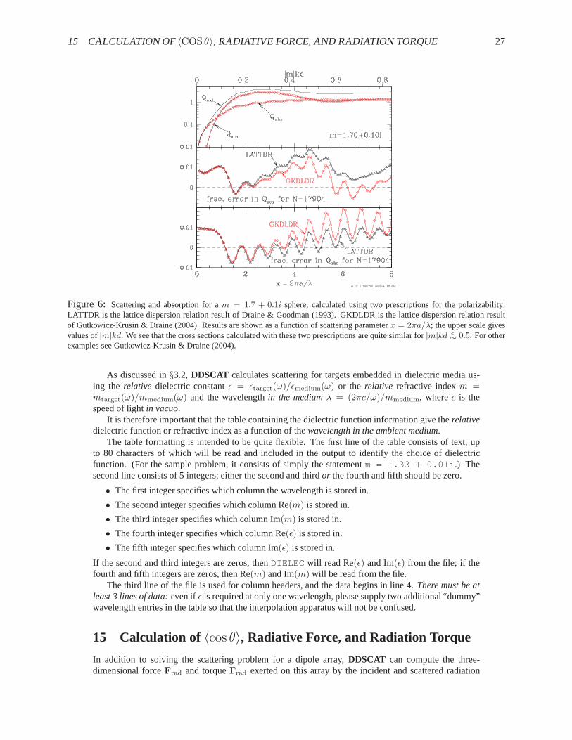
Option GKDLDRspecifies that the polarizability be prescribed by the “Lattice Dispersion Relation”,with the polarizability found by Gutkowicz-Krusin & Draine(2004), who corrected a subtle error in theanalysis of Draine & Goodman (1993). For|m|kd <∼ 1, theGKDLDRpolarizability differs slightly fromtheLATTDRpolarizability, but the differences in calculated scattering cross sections are relatively small,as can be seen from Figure 6. We recommend optionGKDLDR.

Users wishing to compare can invoke optionLATTDRto specify that the “Lattice Dispersion Rela-tion” of Draine & Goodman (1993) be employed to determine thedipole polarizabilities. This polariz-ability also works well.

14 Dielectric Functions

In order to assign the appropriate dipole polarizabilities, DDSCAT 7.0 must be given the dielectricconstant of the material (or materials) of which the target of interest is composedrelative to the dielectricconstant of the ambient medium. This information is supplied toDDSCAT 7.0through a table (or tables),read by subroutineDIELEC in file dielec.f90 , and providing either the complex refractive indexm = n + ik or complex dielectric functionǫ = ǫ1 + iǫ2 as a function of wavelengthλ. Sincem = ǫ1/2,or ǫ = m2, the user must supply eitherm or ǫ.

DDSCAT 7.0can calculate scattering and absorption by targets with anisotropic dielectric functions,with arbitrary orientation of the optical axes relative to the target shape. See§26.

15 CALCULATION OF 〈COS θ〉, RADIATIVE FORCE, AND RADIATION TORQUE 27

Figure 6: Scattering and absorption for am = 1.7 + 0.1i sphere, calculated using two prescriptions for the polarizability:LATTDR is the lattice dispersion relation result of Draine &Goodman (1993). GKDLDR is the lattice dispersion relation resultof Gutkowicz-Krusin & Draine (2004). Results are shown as a function of scattering parameterx = 2πa/λ; the upper scale givesvalues of|m|kd. We see that the cross sections calculated with these two prescriptions are quite similar for|m|kd <

∼ 0.5. For otherexamples see Gutkowicz-Krusin & Draine (2004).

As discussed in§3.2, DDSCAT calculates scattering for targets embedded in dielectric media us-ing the relative dielectric constantǫ = ǫtarget(ω)/ǫmedium(ω) or the relative refractive indexm =mtarget(ω)/mmedium(ω) and the wavelengthin the mediumλ = (2πc/ω)/mmedium, wherec is thespeed of lightin vacuo.

It is therefore important that the table containing the dielectric function information give therelativedielectric function or refractive index as a function of thewavelength in the ambient medium.

The table formatting is intended to be quite flexible. The first line of the table consists of text, upto 80 characters of which will be read and included in the output to identify the choice of dielectricfunction. (For the sample problem, it consists of simply thestatementm = 1.33 + 0.01i .) Thesecond line consists of 5 integers; either the second and third or the fourth and fifth should be zero.

• The first integer specifies which column the wavelength is stored in.

• The second integer specifies which column Re(m) is stored in.

• The third integer specifies which column Im(m) is stored in.

• The fourth integer specifies which column Re(ǫ) is stored in.

• The fifth integer specifies which column Im(ǫ) is stored in.

If the second and third integers are zeros, thenDIELEC will read Re(ǫ) and Im(ǫ) from the file; if thefourth and fifth integers are zeros, then Re(m) and Im(m) will be read from the file.

The third line of the file is used for column headers, and the data begins in line 4.There must be atleast 3 lines of data:even ifǫ is required at only one wavelength, please supply two additional “dummy”wavelength entries in the table so that the interpolation apparatus will not be confused.

15 Calculation of 〈cos θ〉, Radiative Force, and Radiation Torque

In addition to solving the scattering problem for a dipole array, DDSCAT can compute the three-dimensional forceFrad and torqueΓrad exerted on this array by the incident and scattered radiation

16 MEMORY REQUIREMENTS 28

fields. The radiation torque calculation is carried out, after solving the scattering problem, only ifDOTORQhas been specified inddscat.par . For each incident polarization mode, the results aregiven in terms of dimensionless efficiency vectorsQpr andQΓ, defined by

Qpr ≡Frad

πa2effurad

, (19)

QΓ ≡ kΓrad

πa2effurad

, (20)

whereFrad andΓrad are the time-averaged force and torque on the dipole array,k = 2π/λ is thewavenumberin vacuo, andurad = E2

0/8π is the time-averaged energy density for an incident planewave with amplitudeE0 cos(ωt + φ). The radiation pressure efficiency vector can be written

Qpr = Qextk − Qscag , (21)

wherek is the direction of propagation of the incident radiation, and the vectorg is the mean directionof propagation of the scattered radiation:

g =1

Csca

∫

dΩdCsca(n, k)

dΩn , (22)

wheredΩ is the element of solid angle in scattering directionn, anddCsca/dΩ is the differential scat-tering cross section. The components ofQpr are reported in the Target Frame:Qpr,1 ≡ Frad · xTF,Qpr,2 ≡ Frad · yTF, Qpr,3 ≡ Frad · zTF.

Equations for the evaluation of the radiative force and torque are derived by Draine & Weingartner(1996). It is important to note that evaluation ofQpr andQΓ involves averaging over scattering directionsto evaluate the linear and angular momentum transport by thescattered wave. This evaluation requiresappropriate choices of the parameterETASCA– see§23.

In addition,DDSCAT calculates〈cos θ〉 [the first component of the vectorg in eq. (22)] and thesecond moment〈cos2 θ〉. These two moments are useful measures of the anisotropy of the scattering.For example, Draine (2003) gives an analytic approximationto the scattering phase function of dustmixtures that is parameterized by the two moments〈cos θ〉 and〈cos2 θ〉.

16 Memory Requirements

The memory requirements are determined by the size of the “computational volume” – this is a rectan-gular region, of sizeNX×NY×NZ that is large enough to contain the target. If using theGPFAFToption,thenNX, NY, NZare also required to have only 2,3, and 5 as prime factors (seefootnote 11).

In single precision, the memory requirement forDDSCAT 7.0 is approximately

(35. + 0.0010× NX× NY× NZ) Mbytes for single precision (23)

(42 + 0.0020× NX× NY× NZ) Mbytes for double precision (24)

Thus, in single precision, a 48×48×48 calculation requires∼146 MBytes.The memory is allocated dynamically – once the target has been created,DDSCAT 7.0 will deter-

mine just how much overall memory is needed, and will allocate it. However, the user must provideinformation (viaddscat.par ) to allow DDSCAT 7.0 to allocate sufficiently large arrays to carry outthe initial target creation. Initially, the only arrays that will be allocated are those related to the targetgeometry, so it is OK to be quite generous in this initial allowance, as the memory required for the targetgeneration step is small compared to the memory required to carry out the full scattering calculation.

17 TARGET ORIENTATION 29

Figure 7:Target orientation in the Lab Frame.x = xLF is the direction of propagation of the incident radiation, and y = yLF

is the direction of the real component (atxLF = 0, t = 0) of the first incident polarization mode. In this coordinatesystem, theorientation of target axisa1 is specified by anglesΘ andΦ. With target axisa1 fixed, the orientation of target axisa2 is thendetermined by angleβ specifying rotation of the target arounda1. Whenβ = 0, a2 lies in thea1,xLF plane.

17 Target Orientation

Recall that we define a “Lab Frame” (LF) in which the incident radiation propagates in the+x direction.For purposes of discussion we will always let unit vectorsxLF, yLF, zLF = xLF × yLF be the threecoordinate axes of the LF.

In ddscat.par one specifies the first polarization statee01 (which obviously must lie in they, zplane in the LF);DDSCAT automatically constructs a second polarization statee02 = xLF× e∗01 orthog-onal toe01. Users will often find it convenient to let polarization vectors e01 = y, e02 = z (althoughthis is not mandatory – see§22).

Recall that definition of a target involves specifying two unit vectors,a1 anda2, which are imagined

17 TARGET ORIENTATION 30

to be “frozen” into the target. We requirea2 to be orthogonal toa1. Therefore we may define a “TargetFrame” (TF) defined by the three unit vectorsa1, a2, anda3 = a1 × a2 .

For example, whenDDSCAT creates a 32×24×16 rectangular solid, it fixesa1 to be along thelongest dimension of the solid, anda2 to be along the next-longest dimension.

Important Note: for periodic targets,DDSCAT 7.0requires that the periodic target havea1 = xTF

anda2 = yTF.Orientation of the target relative to the incident radiation can in principle be determined two ways:

1. specifying the direction ofa1 anda2 in the LF, or

2. specifying the directions ofxLF (incidence direction) andyLF in the TF.

DDSCAT uses method 1.: the anglesΘ, Φ, andβ are specified in the fileddscat.par . The target isoriented such that the polar anglesΘ andΦ specify the direction ofa1 relative to the incident directionxLF, where thexLF,yLF plane hasΦ = 0. Once the direction ofa1 is specified, the angleβ thenspecifies how the target is to rotated around the axisa1 to fully specify its orientation. A more extendedand precise explanation follows:

17.1 Orientation of the Target in the Lab Frame

DDSCAT uses three angles,Θ, Φ, andβ, to specify the directions of unit vectorsa1 anda2 in the LF(see Fig. 7).

Θ is the angle betweena1 andxLF.WhenΦ = 0, a1 will lie in the xLF, yLF plane. WhenΦ is nonzero, it will refer to the rotation ofa1

aroundxLF: e.g.,Φ = 90 putsa1 in thexLF, zLF plane.Whenβ = 0, a2 will lie in the xLF, a1 plane, in such a way that whenΘ = 0 andΦ = 0, a2 is in

the yLF direction: e.g,Θ = 90, Φ = 0, β = 0 hasa1 = yLF anda2 = −xLF. Nonzeroβ introducesan additional rotation ofa2 arounda1: e.g.,Θ = 90, Φ = 0, β = 90 hasa1 = yLF anda2 = zLF.

Mathematically:

a1 = xLF cosΘ + yLF sinΘ cosΦ + zLF sinΘ sin Φ (25)

a2 = −xLF sin Θ cosβ + yLF[cosΘ cosβ cosΦ − sin β sin Φ]

+zLF[cosΘ cosβ sin Φ + sin β cosΦ] (26)

a3 = xLF sin Θ sinβ − yLF[cosΘ sinβ cosΦ + cosβ sinΦ]

−zLF[cosΘ sinβ sinΦ − cosβ cosΦ] (27)

or, equivalently:

xLF = a1 cosΘ − a2 sin Θ cosβ + a3 sin Θ sinβ (28)

yLF = a1 sin Θ cosΦ + a2[cosΘ cosβ cosΦ − sin β sin Φ]

−a3[cos Θ sinβ cosΦ + cosβ sin Φ] (29)

zLF = a1 sin Θ sinΦ + a2[cosΘ cosβ sin Φ + sinβ cosΦ]

−a3[cos Θ sinβ sin Φ − cosβ cosΦ] (30)

17.2 Orientation of the Incident Beam in the Target Frame

Under some circumstances, one may wish to specify the targetorientation such thatxLF (the directionof propagation of the radiation) andyLF (usually the first polarization direction) andzLF (= xLF ×yLF) refer to certain directions in the TF. Given the definitionsof the LF and TF above, this is simplyan exercise in coordinate transformation. For example, onemight wish to have the incident radiationpropagating along the (1,1,1) direction in the TF (example 14 below). Here we provide some selectedexamples:

1. xLF = a1, yLF = a2, zLF = a3 : Θ = 0, Φ + β = 0

2. xLF = a1, yLF = a3, zLF = −a2 : Θ = 0, Φ + β = 90

18 ORIENTATIONAL AVERAGING 31

3. xLF = a2, yLF = a1, zLF = −a3 : Θ = 90, β = 180, Φ = 0

4. xLF = a2, yLF = a3, zLF = a1 : Θ = 90, β = 180, Φ = 90

5. xLF = a3, yLF = a1, zLF = a2 : Θ = 90, β = −90, Φ = 0

6. xLF = a3, yLF = a2, zLF = −a1 : Θ = 90, β = −90, Φ = −90

7. xLF = −a1, yLF = a2, zLF = −a3 : Θ = 180, β + Φ = 180

8. xLF = −a1, yLF = a3, zLF = a2 : Θ = 180, β + Φ = 90

9. xLF = −a2, yLF = a1, zLF = a3 : Θ = 90, β = 0, Φ = 0

10. xLF = −a2, yLF = a3, zLF = −a1 : Θ = 90, β = 0, Φ = −90

11. xLF = −a3, yLF = a1, zLF = −a2 : Θ = 90, β = −90, Φ = 0

12. xLF = −a3, yLF = a2, zLF = a1 : Θ = 90, β = −90, Φ = 90

13. xLF = (a1 + a2)/√

2, yLF = a3, zLF = (a1 − a2)/√

2 : Θ = 45, β = 180, Φ = 90

14. xLF = (a1 + a2 + a3)/√

3, yLF = (a1 − a2)/√

2, zLF = (a1 + a2 − 2a3)/√

6 :Θ = 54.7356, β = 135, Φ = 30.

17.3 Sampling inΘ, Φ, and β

The present version,DDSCAT 7.0, chooses the anglesβ, Θ, andΦ to sample the intervals (BETAMI,BETAMX),(THETMI,THETMX), (PHIMIN,PHIMAX ), whereBETAMI, BETAMX, THETMI, THETMX, PHIMIN ,PHIMAXare specified inddscat.par . The prescription for choosing the angles is to:

• uniformly sample inβ;

• uniformly sample inΦ;

• uniformly sample incosΘ.

This prescription is appropriate for random orientation ofthe target, within the specified limits ofβ, Φ,andΘ.

Note that whenDDSCAT 7.0chooses angles it handlesβ andΦ differently fromΘ. The range forβis divided intoNBETAintervals, and the midpoint of each interval is taken. Thus,if you takeBETAMI=0,BETAMX=90,NBETA=2 you will getβ = 22.5 and67.5. Similarly, if you takePHIMIN=0,PHIMAX=180,NPHI=2 you will getΦ = 45 and135.

Sampling inΘ is done quite differently from sampling inβ andΦ. First, as already mentioned above,DDSCAT 7.0samples uniformly incosΘ, notΘ. Secondly, the sampling depends on whetherNTHETAis even or odd.

• If NTHETAis odd, then the values ofΘ selected include the extreme valuesTHETMIandTHETMX;thus,THETMI=0,THETMX=90,NTHETA=3 will give youΘ = 0, 60, 90.

• If NTHETAis even, then the range ofcosΘ will be divided intoNTHETAintervals, and the mid-point of each interval will be taken; thus,THETMI=0, THETMX=90, NTHETA=2 will give youΘ = 41.41 and75.52 [cosΘ = 0.25 and0.75].

The reason for this is that if oddNTHETAis specified, then the “integration” overcosΘ is performedusing Simpson’s rule for greater accuracy. If evenNTHETAis specified, then the integration overcosΘis performed by simply taking the average of the results for the differentΘ values.

If averaging over orientations is desired, it is recommended that the user specify anodd value ofNTHETAso that Simpson’s rule will be employed.

18 Orientational Averaging

DDSCAT has been constructed to facilitate the computation of orientational averages. How to go aboutthis depends on the distribution of orientations which is applicable.

19 TARGET GENERATION: ISOLATED FINITE TARGETS 32

18.1 Randomly-Oriented Targets

For randomly-oriented targets, we wish to compute the orientational average of a quantityQ(β, Θ, Φ):

〈Q〉 =1

8π2

∫ 2π

0

dβ

∫ 1

−1

d cosΘ

∫ 2π

0

dΦ Q(β, Θ, Φ) . (31)

To compute such averages, all you need to do is edit the fileddscat.par so that DDSCAT knowswhat ranges of the anglesβ, Θ, andΦ are of interest. For a randomly-oriented target with no symmetry,you would need to letβ run from 0 to360, Θ from 0 to180, andΦ from 0 to360.

For targets with symmetry, on the other hand, the ranges ofβ, Θ, andΦ may be reduced. Firstof all, remember that averaging overΦ is relatively “inexpensive”, so when in doubt average over 0to360; most of the computational “cost” is associated with the number of different values of (β,Θ) whichare used. Consider a cube, for example, with axisa1 normal to one of the cube faces; for this cubeβneed run only from 0 to90, since the cube has fourfold symmetry for rotations around the axisa1.Furthermore, the angleΘ need run only from 0 to90, since the orientation (β,Θ,Φ) is indistinguishablefrom (β, 180 − Θ, 360 − Φ).

For targets with symmetry, the user is encouraged to test thesignificance ofβ,Θ,Φ on targets withsmall numbers of dipoles (say, of the order of 100 or so) but having the desired symmetry.

18.2 Nonrandomly-Oriented Targets

Some special cases (where the target orientation distribution is uniform for rotations around thex axis =direction of propagation of the incident radiation), one may be able to useDDSCAT 7.0with appropriatechoices of input parameters. More generally, however, you will need to modify subroutineORIENT togenerate a list ofNBETAvalues ofβ, NTHETAvalues ofΘ, andNPHI values ofΦ, plus two weight-ing arraysWGTA(1-NTHETA,1-NPHI) andWGTB(1-NBETA). HereWGTAgives the weights whichshould be attached to each (Θ,Φ) orientation, andWGTBgives the weight to be attached to eachβ ori-entation. Thus each orientation of the target is to be weighted by the factorWGTA×WGTB. For the caseof random orientations,DDSCAT choosesΘ values which are uniformly spaced incosΘ, andβ andΦvalues which are uniformly spaced, and therefore uses uniform weights

WGTB=1./NBETA

WhenNTHETAis even,DDSCAT setsWGTA=1./(NTHETA×NPHI)

but whenNTHETAis odd,DDSCAT uses Simpson’s rule when integrating overΘ andWGTA= (1/3 or 4/3 or 2/3)/(NTHETA×NPHI)

Note that the program structure ofDDSCAT may not be ideally suited for certain highly orientedcases. If, for example, the orientation is such that for a given Φ value only oneΘ value is possible(this situation might describe ice needles oriented with the long axis perpendicular to the vertical in theEarth’s atmosphere, illuminated by the Sun at other than thezenith) then it is foolish to consider all thecombinations ofΘ andΦ which the present version ofDDSCAT is set up to do. We hope to improvethis in a future version ofDDSCAT.

19 Target Generation: Isolated Finite Targets

DDSCAT contains routines to generate dipole arrays representing finite targets of various geometries,including spheres, ellipsoids, rectangular solids, cylinders, hexagonal prisms, tetrahedra, two touchingellipsoids, and three touching ellipsoids. The target typeis specified by variableCSHAPEon line 9 ofddscat.par , up to 12 target shape parameters (SHPAR1, SHPAR2, SHPAR3, ...) on line 10. Thetarget geometry is most conveniently described in a coordinate system attached to the target which werefer to as the “Target Frame” (TF), with orthonormal unit vectorsxTF, yTF, zTF ≡ xTF × yTF. Oncethe target is generated, the orientation of the target in theLab Frame is accomplished as described in§17.

Every target generation routine will specify

19 TARGET GENERATION: ISOLATED FINITE TARGETS 33

• The “occupied” lattice sites;

• The composition associated with each occupied lattice site;

• Two “target axes”a1 anda2 that are used as references when specifying the target orientation; and

• The location of the Target Frame origin of coordinates.

Target geometries currently supported include:

19.1 FROM FILE = Target composed of possibly anisotropic material, definedby list of dipole locations and “compositions” obtained from a file

If anisotropic, the “microcrystals” in the target are assumed to be aligned with the principal axes ofthe dielectric tensor parallel toxTF, yTF, and zTF. This option causesDDSCAT to read the targetgeometry and composition information from a fileshape.dat instead of automatically generatingone of the geometries for which DDSCAT has built-in target generation capability. Theshape.datfile is read by routineREASHP(file reashp.f90 ). The file shape.dat gives the numberN ofdipoles in the target, the components of the “target axes”a1 anda2 in the Target Frame (TF), the vectorx0(1 − 3) determining the correspondence between the integersIXYZ and actual coordinates in the TF,and specifications for the location and “composition” of each dipole. The user can customizeREASHPasneeded to conform to the manner in which the target description is stored in fileshape.dat . However,as supplied,REASHPexpects the fileshape.dat to have the following structure:

• one line containing a description; the first 67 characters will be read and printed in various outputstatements

• N= number of dipoles in target

• a1x a1y a1z = x,y,z components (in TF) ofa1

• a2x a2y a2z = x,y,z components (in TF) ofa2

• dx/d dy/d dz/d = 1. 1. 1. = relative spacing of dipoles inxTF, yTF, zTF directions

• x0x x0y x0z = TF coordinatesxTF/d yTF/d zTF/d corresponding to lattice siteIXYZ = 0 0 0

• (line containing comments)

• dummy IXYZ(1,1) IXYZ(1,2) IXYZ(1,3) ICOMP(1,1) ICOMP(1,2) ICOM P(1,3)

• dummy IXYZ(2,1) IXYZ(2,2) IXYZ(2,3) ICOMP(2,1) ICOMP(2,2) ICOM P(2,3)

• dummy IXYZ(3,1) IXYZ(3,2) IXYZ(3,3) ICOMP(3,1) ICOMP(3,2) ICOM P(3,3)

• ...

• dummy IXYZ(J,1) IXYZ(J,2) IXYZ(J,3) ICOMP(J,1) ICOMP(J,2) ICOM P(J,3)

• ...

• dummy IXYZ(N,1) IXYZ(N,2) IXYZ(N,3) ICOMP(N,1) ICOMP(N,2) ICOM P(N,3)

wheredummy is a string that does not contain spaces, commas, or other separators.If the target material at locationJ is isotropic,ICOMP(J,1) , ICOMP(J,2) , andICOMP(J,3) havethe same value.

19.2 ANIFRMFIL = General anistropic target defined by list of dipole locations,“compositions”, and material orientations obtained from a file

This option causesDDSCAT to read the target geometry information from a fileshape.dat insteadof automatically generating one of the geometries listed below. The fileshape.dat gives the num-ber N of dipoles in the target, the components of the “target axes”a1 and a2 in the Target Frame(TF), the vectorx0(1 − 3) determining the correspondence between the integersIXYZ and actual co-ordinates in the TF, and specifications for the location and “composition” of each dipole. For eachdipoleJ , the fileshape.dat provides the locationIXYZ( J ,1-3) , the composition identifier integer

19 TARGET GENERATION: ISOLATED FINITE TARGETS 34

ICOMP(J ,1-3) specifying the dielectric function corresponding to the three principal axes of the di-electric tensor, and anglesΘDF, ΦDF, andβDF specifying the orientation of the local “Dielectric Frame”(DF) relative to the “Target Frame” (TF) (see§26). The DF is the reference frame in which the dielectrictensor is diagonalized. The Target Frame is the reference frame in which we specify the dipole locations.

The shape.dat file is read by routineREASHP(file reashp.f90 ). The user can customizeREASHPas needed to conform to the manner in which the target geometry is stored in fileshape.dat .However, as supplied,REASHPexpects the fileshape.dat to have the following structure:

• one line containing a description; the first 67 characters will be read and printed in various outputstatements.

• N= number of dipoles in target

• a1x a1y a1z = x,y,z components (in Target Frame) ofa1

• a2x a2y a2z = x,y,z components (in Target Frame) ofa2

• dx/d dy/d dz/d = 1. 1. 1. = relative spacing of dipoles inxTF, yTF, zTF directions

• x0x x0y x0z = TF coordinatesxTF/d yTF/d zTF/d corresponding to lattice siteIXYZ = 0 0 0

• (line containing comments)

• dummy IXYZ(1,1-3) ICOMP(1,1-3) THETADF(1) PHIDF(1) BETADF(1)

• dummy IXYZ(2,1-3) ICOMP(2,1-3) THETADF(2) PHIDF(2) BETADF(2)

• dummy IXYZ(3,1-3) ICOMP(3,1-3) THETADF(3) PHIDF(3) BETADF(3)

• ...

• dummy IXYZ(J,1-3) ICOMP(J,1-3) THETADF(J) PHIDF(J) BETADF(J)

• ...

• dummy IXYZ(N,1-3) ICOMP(N,1-3) THETADF(N) PHIDF(N) BETADF(N)

Wheredummy is a string that does not contain spaces, commas, or other separators.THETADF PHIDFBETADFshould be given in degrees.

19.3 ANIELLIPS = Homogeneous, anisotropic ellipsoid.

SHPAR1, SHPAR2, SHPAR3 define the ellipsoidal boundary:

(

xTF/d

SHPAR1

)2

+

(

yTF/d

SHPAR2

)2

+

(

zTF/d

SHPAR3

)2

=1

4, (32)

The TF origin is located at the centroid of the ellipsoid.

19.4 ANI ELL 2 = Two touching, homogeneous, anisotropic ellipsoids, with dis-tinct compositions

Geometry as forELLIPSO 2; SHPAR1, SHPAR2, SHPAR3 have same meanings as forELLIPSO 2.Target axesa1 = (1, 0, 0)TF anda2 = (0, 1, 0)TF.Line connecting ellipsoid centers is‖ a1 = xTF.TF origin is located between ellipsoids, at point of contact.It is assumed that (for both ellipsoids) the dielectric tensor is diagonal in the TF. User must setNCOMP=6and providexx, yy, zz components of dielectric tensor for first ellipsoid, andxx, yy, zz components ofdielectric tensor for second ellipsoid (ellipsoids are in order of increasingxTF).

19 TARGET GENERATION: ISOLATED FINITE TARGETS 35

19.5 ANI ELL 3 = Three touching homogeneous, anisotropic ellipsoids withsame size and orientation but distinct dielectric tensors

SHPAR1, SHPAR2, SHPAR3 have same meanings as forELLIPSO 3.Target axisa1 = (1, 0, 0)TF (along line of ellipsoid centers), anda2 = (0, 1, 0)TF.TF origin is located at center of middle ellipsoid.It is assumed that dielectric tensors are all diagonal in theTF. User must setNCOMP=9 and providexx,yy, zz elements of dielectric tensor for first ellipsoid,xx, yy, zz elements for second ellipsoid, andxx,yy, zz elements for third ellipsoid (ellipsoids are in order of increasingxTF).

19.6 ANIRCTNGL = Homogeneous, anisotropic, rectangular solidx, y, z lengths/d = SHPAR1, SHPAR2, SHPAR3.Target axesa1 = (1, 0, 0)TF anda2 = (0, 1, 0)TF in the TF.(xTF, yTF, zTF) = (0, 0, 0) at middle of upper target surface, (where “up” =xTF). (The target surfaceis taken to bed/2 about the upper dipole layer.)Dielectric tensor is assumed to be diagonal in the target frame.User must setNCOMP=3 and supply names of three files forǫ as a function of wavelength or energy: firstfor ǫxx, second forǫyy, and third forǫzz, as in the following sampleddscat.par file:

’ =================== Parameter file ================== =’’ **** PRELIMINARIES **** ’’NOTORQ’= CMTORQ* 6 (DOTORQ, NOTORQ) -- either do or skip torque calculations’PBCGS2’= CMDSOL* 6 (PBCGS2, PBCGST, PETRKP) -- select solution method’GPFAFT’= CMETHD* 6 (GPFAFT, FFTMKL)’GKDLDR’= CALPHA* 6 (GKDLDR, LATTDR)’NOTBIN’= CBINFLAG (ALLBIN, ORIBIN, NOTBIN)’ANIRCTNGL’= CSHAPE* 9 shape directive’ **** Initial Memory Allocation **** ’10 25 50 = upper bound on target extent’ **** Target Geometry and Composition **** ’’ANIRCTNGL’= CSHAPE* 9 shape directive10 25 50 = shape parameters SHPAR1, SHPAR2, SHPAR33 = NCOMP = number of dielectric materials’/u/draine/DDA/diel/m2.00_0.10’ = name of file containin g dielectric function’/u/draine/DDA/diel/m1.50_0.00’’/u/draine/DDA/diel/m1.50_0.00’’ **** Error Tolerance **** ’1.00e-5 = TOL = MAX ALLOWED (NORM OF |G>=AC|E>-ACA|X>)/(NORM OF AC|E>)’ **** Interaction cutoff parameter for PBC calculations **** ’5.00e-3 = GAMMA (1e-2 is normal, 3e-3 for greater accuracy)’ **** Angular resolution for calculation of <cos>, etc. **** ’2.0 = ETASCA (number of angles is proportional to [(2+x)/ETA SCA]ˆ2 )’ **** Wavelengths (micron) **** ’500. 500. 1 ’INV’ = wavelengths (first,last,how many,how=L IN,INV,LOG)’ **** Effective Radii (micron) **** ’30.60 30.60 1 ’LIN’ = eff. radii (first, last, how many, how=L IN,INV,LOG)’ **** Define Incident Polarizations **** ’(0,0) (1.,0.) (0.,0.) = Polarization state e01 (k along x axi s)2 = IORTH (=1 to do only pol. state e01; =2 to also do orth. pol. s tate)’ **** Specify which output files to write **** ’1 = IWRKSC (=0 to suppress, =1 to write ".sca" file for each tar get orient.1 = IWRPOL (=0 to suppress, =1 to write ".pol" file for each (BE TA,THETA)’ **** Prescribe Target Rotations **** ’

0. 0. 1 = BETAMI, BETAMX, NBETA (beta=rotation around a1)0. 90. 3 = THETMI, THETMX, NTHETA (theta=angle between a1 and k)0. 0. 1 = PHIMIN, PHIMAX, NPHI (phi=rotation angle of a1 aroun d k)

’ **** Specify first IWAV, IRAD, IORI (normally 0 0 0) **** ’0 0 0 = first IWAV, first IRAD, first IORI (0 0 0 to begin fresh)’ **** Select Elements of S_ij Matrix to Print **** ’6 = NSMELTS = number of elements of S_ij to print (not more than 9)11 12 21 22 31 41 = indices ij of elements to print’ **** Specify Scattered Directions **** ’’LFRAME’ = CMDFRM* 6 (’LFRAME’ or ’TFRAME’ for Lab Frame or Target Frame)2 = NPLANES = number of scattering planes

19 TARGET GENERATION: ISOLATED FINITE TARGETS 36

0. 0. 180. 30 = phi, thetan_min, thetan_max, dtheta (in degre es) for plane A90. 0. 180. 30 = phi, ... for plane B

19.7 CONELLIPS = Two concentric ellipsoids

SHPAR1, SHPAR2, SHPAR3 = lengths/d of theouterellipsoid along thexTF, yTF, zTF axes;SHPAR4, SHPAR5, SHPAR6 = lengths/d of the innerellipsoid along thexTF, yTF, zTF axes.Target axesa1 = (1, 0, 0)TF, a2 = (0, 1, 0)TF.TF origin is located at centroids of ellipsoids.The “core” within the inner ellipsoid is composed of isotropic material 1; the “mantle” between innerand outer ellipsoids is composed of isotropic material 2.User must setNCOMP=2 and provide dielectric functions for “core” and “mantle”materials.

19.8 CYLINDER1 = Homogeneous, isotropic finite cylinder

SHPAR1 = length/d, SHPAR2 = diameter/d, withSHPAR3 = 1 for cylinder axisa1 ‖ xTF: a1 = (1, 0, 0)TF anda2 = (0, 1, 0)TF;SHPAR3 = 2 for cylinder axisa1 ‖ yTF: a1 = (0, 1, 0)TF anda2 = (0, 0, 1)TF;SHPAR3 = 3 for cylinder axisa1 ‖ zTF: a1 = (0, 0, 1)TF anda2 = (1, 0, 0)TF in the TF.TF origin is located at centroid of cylinder.User must setNCOMP=1.

19.9 CYLNDRCAP = Homogeneous, isotropic finite cylinder with hemispheri-cal endcaps.

SHPAR1 = cylinder length/d (not including end-caps!) andSHPAR2 = cylinder diameter/d, with cylinderaxis = a1 = (1, 0, 0)TF and a2 = (0, 1, 0)TF. The total length along the target axis (including theendcaps) is (SHPAR1+SHPAR2)d.TF origin is located at centroid of cylinder.User must setNCOMP=1.

19.10 DSKRCTNGL = Disk on top of a homogeneous rectangular slab

This option causesDDSCAT to create a target consisting of a disk of composition 1 resting on top of arectangular block of composition 2. Materials 1 and 2 are assumed to be homogeneous and isotropic.ddscat.par should setNCOMPto 2 .The cylindrical disk has thicknessSHPAR1×d in the x-direction, and diameterSHPAR2×d. The rect-angular block is assumed to have thicknessSHPAR3×d in the x-direction, lengthSHPAR4×d in they-direction, and lengthSHPAR5×d in the z-direction. The lower surface of the cylindrical disk is in thex = 0 plane. The upper surface of the slab is also in thex = 0 plane.

The Target Frame origin (0,0,0) is located where the symmetry axis of the disk intersects thex = 0plane (the upper surface of the slab, and the lower surface ofthe disk). In the Target Frame, dipolesrepresenting the rectangular block are located at(x/d, y/d, z/d) = (jx + 0.5, jy + ∆y, jz + ∆z), wherejx, jy, andjz are integers.∆y = 0 or 0.5 depending on whetherSHPAR4 is even or odd.∆z = 0 or 0.5depending on whetherSHPAR5 is even or odd.

Dipoles representing the disk are located atx/d = 0.5, 1.5, ..., [int(SHPAR4 + 0.5)− 0.5]

As always, the physical size of the target is fixed by specifying the value of the effective radiusaeff ≡ (3VTUC/4π)1/3, whereVTUC is the total volume of solid material in one TUC. For this geom-etry, the number of dipoles in the target will be approximately N = [SHPAR1 × SHPAR2 × SHPAR3 +(π/4)((SHPAR4)

2 × SHPAR5)], although the exact number may differ because of the dipolesare requiredto be located on a rectangular lattice. The dipole spacingd in physical units is determined from thespecified value ofaeff and the numberN of dipoles in the target:d = (4π/3N)1/3aeff . This optionrequires 5 shape parameters:

19 TARGET GENERATION: ISOLATED FINITE TARGETS 37

The pertinent line inddscat.par should read

SHPAR1 SHPAR2 SHPAR3 SHPAR4 SHPAR5

whereSHPAR1 = [disk thickness (inxTF direction)]/d [material 1]SHPAR2 = (disk diameter)/dSHPAR3 = (brick thickness inxTF direction)/d [material 2]SHPAR4 = (brick thickness inyTF direction)/dSHPAR5 = (brick thickness inzTF direction)/d

The overall size of the TUC (in terms of numbers of dipoles) isdetermined by parameters(SHPAR1+SHPAR4),SHPAR2, andSHPAR3. The periodicity in the TFy andz directions is determined by parametersSHPAR4andSHPAR5.The physical size of the TUC is specified by the value ofaeff (in physical units, e.g. cm), specified in thefile ddscat.par .

The “computational volume” is determined by (SHPAR1+SHPAR4)×SHPAR2×SHPAR3.The target axes (in the TF) are set toa1 = xTF = (1, 0, 0)TF – i.e., normal to the “slab” – and

a2 = yTF = (0, 1, 0)TF. The orientation of the incident radiation relative to the target is, as for all othertargets, set by the usual orientation anglesβ, Θ, andΦ (see§17 above); for example,Θ = 0 would befor radiation incident normal to the slab.

19.11 DW1996TAR = 13 block target used by Draine & Weingartner (1996).

Single, isotropic material. Target geometry was used in study by Draine & Weingartner (1996) of radia-tive torques on irregular grains.a1 anda2 are principal axes with largest and second-largest momentsofinertia. User must setNCOMP=1. Target size is controlled by shape parameterSHPAR(1) = width ofone block in lattice units.TF origin is located at centroid of target.

19.12 ELLIPSOID = Homogeneous, isotropic ellipsoid.

“Lengths”SHPAR1, SHPAR2, SHPAR3 in thex, y, z directions in the TF:

(

xTF

SHPAR1d

)2

+

(

yTF

SHPAR2d

)2

+

(

zTF

SHPAR3d

)2

=1

4, (33)

whered is the interdipole spacing.The target axes are set toa1 = (1, 0, 0)TF anda2 = (0, 1, 0)TF.Target Frame origin = centroid of ellipsoid.User must setNCOMP=1 on line 9 ofddscat.par .A homogeneous, isotropic sphereis obtained by settingSHPAR1 = SHPAR2 = SHPAR3 = diameter/d.

19.13 ELLIPSO 2 = Two touching, homogeneous, isotropic ellipsoids, with dis-tinct compositions

SHPAR1, SHPAR2, SHPAR3=x-length/d, y-length/d, z-length/d of one ellipsoid. The two ellipsoidshave identical shape, size, and orientation, but distinct dielectric functions. The line connecting ellipsoidcenters is along thexTF-axis. Target axesa1 = (1, 0, 0)TF [along line connecting ellipsoids] anda2 = (0, 1, 0)TF.Target Frame origin = midpoint between ellipsoids (where ellipsoids touch).User must setNCOMP=2 and provide dielectric function file names for both ellipsoids. Ellipsoids arein order of increasingxTF: first dielectric function is for ellipsoid with center at negativexTF, seconddielectric function for ellipsoid with center at positivexTF.

19 TARGET GENERATION: ISOLATED FINITE TARGETS 38

19.14 ELLIPSO 3 = Three touching homogeneous, isotropic ellipsoids of equalsize and orientation, but distinct compositions

SHPAR1, SHPAR2, SHPAR3 have same meaning as forELLIPSO 2. Line connecting ellipsoid centers isparallel toxTF axis. Target axisa1 = (1, 0, 0)TF (along line of ellipsoid centers), anda2 = (0, 1, 0)TF.Target Frame origin = centroid of middle ellipsoid.User must setNCOMP=3 and provide (isotropic) dielectric functions for first, second, and third ellipsoid.

19.15 HEX PRISM = Homogeneous, isotropic hexagonal prism

SHPAR1 = (Length of prism)/d = (distance between hexagonal faces)/d,SHPAR2 = (distance between opposite vertices of one hexagonal face)/d = 2×hexagon side/d.SHPAR3 selects one of 6 orientations of the prism in the Target Frame(TF).Target axisa1 is along the prism axis (i.e., normal to the hexagonal faces), and target axisa2 is normalto one of the rectangular faces. There are 6 options forSHPAR3:SHPAR3 = 1 for a1 ‖ xTF anda2 ‖ yTF ; SHPAR3 = 2 for a1 ‖ xTF anda2 ‖ zTF ;SHPAR3 = 3 for a1 ‖ yTF anda2 ‖ xTF ; SHPAR3 = 4 for a1 ‖ yTF anda2 ‖ zTF ;SHPAR3 = 5 for a1 ‖ zTF anda2 ‖ xTF ; SHPAR3 = 6 for a1 ‖ zTF anda2 ‖ yTF

TF origin is located at the centroid of the target.User must setNCOMP=1.

19.16 LAYRDSLAB = Multilayer rectangular slab

Multilayer rectangular slab with overall x, y, z lengthsax = SHPAR1 × day = SHPAR2 × d,az = SHPAR3 × d.Upper surface is atxTF = 0, lower surface atxTF = −SHPAR1 × dSHPAR4 = fraction which is composition 1 (top layer).SHPAR5 = fraction which is composition 2 (layer below top)SHPAR6 = fraction which is composition 3 (layer below comp 2)1 − (SHPAR4 + SHPAR5 + SHPAR6) = fraction which is composition 4 (bottom layer).To create a bilayer slab, just setSHPAR5 = SHPAR6 = 0To create a trilayer slab, just setSHPAR6 = 0User must setNCOMP=2,3, or 4 and provide dielectric function files for each of the two layers. Topdipole layer is atxTF = −d/2. Origin of TF is at center of top surface.

19.17 MLTBLOCKS = Homogeneous target constructed from cubic “blocks”

Number and location of blocks are specified in separate fileblocks.par with following structure:one line of comments (may be blank)PRIN (= 0 or 1 – see below)N (= number of blocks)B (= width/d of one block)xTF yTF zTF (= position of 1st block in units ofBd)xTF yTF zTF (= position of 2nd block in units ofBd) )...xTF yTF zTF (= position ofNth block in units ofBd)

If PRIN=0, thena1 = (1, 0, 0)TF, a2 = (0, 1, 0)TF. If PRIN=1, thena1 anda2 are set to principal axeswith largest and second largest moments of inertia, assuming target to be of uniform density. User mustsetNCOMP=1.

19 TARGET GENERATION: ISOLATED FINITE TARGETS 39

19.18 RCTGLPRSM = Homogeneous, isotropic, rectangular solid

x, y, z lengths/d = SHPAR1, SHPAR2, SHPAR3.Target axesa1 = (1, 0, 0)TF anda2 = (0, 1, 0)TF.TF origin at center of upper surface of solid: target extendsfrom xTF/d = −SHPAR1 to 0,yTF/d from−0.5 × SHPAR2 to +0.5 × SHPAR2

zTF/d from−0.5 × SHPAR3 to +0.5 × SHPAR3

User must setNCOMP=1.

19.19 RCTGLBLK3 = Stack of 3 rectangular blocks, with centers on the xTF

axis.

Each block consists of a distinct material. There are 9 shapeparameters:SHPAR1 = (upper solid thickness inxTF direction)/d [material 1]SHPAR2 = (upper solid width inyTF direction)/dSHPAR3 = (upper solid width inzTF direction)/dSHPAR4 = (middle solid thickness inxTF direction)/d [material 2]SHPAR5 = (middle solid width inyTF direction)/dSHPAR6 = (middle solid width inzTF direction)/dSHPAR7 = (lower solid thickness inxTF direction)/d [material 3]SHPAR8 = (lower solid width inyTF direction)/dSHPAR9 = (lower solid width inzTF direction)/dTF origin is at center of top surface of material 1.

19.20 SPHERESN = Multisphere target = union of N spheres of single isotropicmaterial

Spheres may overlap if desired. The relative locations and sizes of these spheres are defined in anexternal file, whose name (enclosed in single quotes) is passed throughddscat.par . The length ofthe file name should not exceed 80 characters. The pertinent line inddscat.par should readSHPAR1 SHPAR2 ‘filename’(quotes must be used)whereSHPAR1 = target diameter inx direction (in Target Frame) in units ofdSHPAR2= 0 to havea1 = (1, 0, 0)TF, a2 = (0, 1, 0)TF.SHPAR2= 1 to use principal axes of moment of inertia tensor fora1 (largestI) anda2 (intermediateI).filenameis the name of the file specifying the locations and relative sizes of the spheres.The overall size of the multisphere target (in terms of numbers of dipoles) is determined by parameterSHPAR(1) , which is the extent of the multisphere target in thex-direction, in units of the lattice spacingd. The file‘filename’should have the following structure:

N (= number of spheres)one line of comments (may be blank)x1 y1 z1 a1 (arb. units)x2 y2 z2 a2 (arb. units)...xN yN zN aN (arb. units)

wherexj , yj, zj are the coordinates (in the TF) of the center, andaj is the radius of spherej.Note thatxj , yj , zj, aj (j = 1, ..., N ) establish only theshapeof theN−sphere target. For instance,a target consisting of two touching spheres with the line between centers parallel to thex axis couldequally well be described by lines 3 and 4 being

0 0 0 0.51 0 0 0.5

or0 0 0 12 0 0 1

The actual size (in physical units) is set by the value ofaeff specified inddscat.par , where, as always,

19 TARGET GENERATION: ISOLATED FINITE TARGETS 40

aeff ≡ (3V/4π)1/3, whereV is the total volume of material in the target.Target axesa1 and a2 are set to be principal axes of moment of inertia tensor (for uniform density),wherea1 corresponds to the largest eigenvalue, anda2 to the intermediate eigenvalue.The TF origin is taken to be located at the volume-weighted centroid.User must setNCOMP=1.

19.21 SPHROID2 = Two touching homogeneous, isotropic spheroids, with dis-tinct compositions

First spheroid has lengthSHPAR1 along symmetry axis, diameterSHPAR2 perpendicular to symmetryaxis. Second spheroid has lengthSHPAR3 along symmetry axis, diameterSHPAR4 perpendicular tosymmetry axis. Contact point is on line connecting centroids. Line connecting centroids is inxTF

direction. Symmetry axis of first spheroid is inyTF direction. Symmetry axis of second spheroid is indirectionyTF cos(SHPAR5) + zTF sin(SHPAR5), andSHPAR5 is in degrees. IfSHPAR6 = 0., then targetaxesa1 = (1, 0, 0)TF, a2 = (0, 1, 0)TF. If SHPAR6 = 1., then axesa1 anda2 are set to principal axeswith largest and 2nd largest moments of inertia assuming spheroids to be of uniform density.Origin of TF is located between spheroids, at point of contact.User must setNCOMP=2 and provide dielectric function files for each spheroid.

19.22 SPHANI N = Multisphere target consisting of the union ofN spheres ofvarious materials, possibly anisotropic

Spheres may NOT overlap. The relative locations and sizes ofthese spheres are defined in an externalfile, whose name (enclosed in single quotes) is passed through ddscat.par . The length of the filename should not exceed 80 characters. Target axesa1 and a2 are set to be principal axes of momentof inertia tensor (for uniform density), wherea1 corresponds to the largest eigenvalue, anda2 to theintermediate eigenvalue.The TF origin is taken to be located at the volume-weighted centroid.The pertinent line inddscat.par should readSHPAR1 SHPAR2 ‘filename’(quotes must be used)whereSHPAR1 = target diameter inx direction (in Target Frame) in units ofdSHPAR2= 0 to havea1 = (1, 0, 0)TF, a2 = (0, 1, 0)TF in Target Frame.SHPAR2= 1 to use principal axes of moment of inertia tensor fora1 (largestI) anda2 (intermediateI).filenameis the name of the file specifying the locations and relative sizes of the spheres.The overall size of the multisphere target (in terms of numbers of dipoles) is determined by parameterSHPAR1, which is the extent of the multisphere target in thex-direction, in units of the lattice spacingd.The file ‘filename’should have the following structure:

N (= number of spheres)one line of comments (may be blank)x1 y1 z1 r1 Cx1 Cy1 Cz1 ΘDF,1 ΦDF,1 βDF,1

x2 y2 z2 r2 Cx2 Cy2 Cz2 ΘDF,2 ΦDF,2 βDF,2

...xN yN zN rN CxN CyN CzN ΘDF,N ΦDF,N βDF,N

wherexj , yj , zj are the coordinates of the center, andrj is the radius of spherej (arbitrary units),Cxj , Cyj , Czj are integers specifying the “composition” of spherej in the x, y, z directions in the“Dielectric Frame” (see§26) of spherej, andΘDF,j ΦDF,j βDF,j are angles (in radians) specifyingorientation of the dielectric frame (DF) of spherej relative to the Target Frame. Note thatxj , yj, zj , rj

(j = 1, ..., N ) establish only theshapeof theN−sphere target, just as for target optionNSPHER. Theactual size (in physical units) is set by the value ofaeff specified inddscat.par , where, as always,aeff ≡ (3V/4π)1/3, whereV is the volume of material in the target.User must setNCOMPto the number of different dielectric functions being invoked (i.e., the range ofCxj , Cyj , Czj.

Note that while the spheres can be anisotropic and of differing composition, they can of course alsobe isotropic and of a single composition, in which case the relevant lines in the file’filename’would be

19 TARGET GENERATION: ISOLATED FINITE TARGETS 41

simplyN (= number of spheres)one line of comments (may be blank)x1 y1 z1 r1 1 1 1 0 0 0x2 y2 z2 r2 1 1 1 0 0 0...xN yN zN rN 1 1 1 0 0 0

19.23 TETRAHDRN = Homogeneous, isotropic tetrahedron

SHPAR1=length/d of one edge. Orientation: one face parallel toyTF, zTF plane, opposite “vertex” isin +xTF direction, and one edge is parallel tozTF. Target axesa1 = (1, 0, 0)TF [emerging from onevertex] anda2 = (0, 1, 0)TF [emerging from an edge] in the TF. User must setNCOMP=1.

19.24 TRNGLPRSM = Triangular prism of homogeneous, isotropic material

SHPAR1, SHPAR2, SHPAR3, SHPAR4 = a/d, b/a, c/a, L/aThe triangular cross section has sides of widtha, b, c. L is the length of the prism.d is the latticespacing. The triangular cross-section has interior anglesα, β, γ (opposite sidesa, b, c) given bycosα =(b2 + c2 − a2)/2bc, cosβ = (a2 + c2 − b2)/2ac, cos γ = (a2 + b2 − c2)/2ab. In the Target Frame,the prism axis is in thex direction, the normal to the rectangular face of widtha is (0,1,0), the normal tothe rectangular face of widthb is (0,− cosγ, sinγ), and the normal to the rectangular face of widthc is(0,− cosγ,− sinγ).

19.25 UNIAXICYL = Homogeneous finite cylinder with uniaxial anisotropic di-electric tensor

SHPAR1, SHPAR2 have same meaning as forCYLINDER1. Cylinder axis= a1 = (1, 0, 0)TF, a2 =(0, 1, 0)TF. It is assumed that the dielectric tensorǫ is diagonal in the TF, withǫyy = ǫzz. User must setNCOMP=2. Dielectric function 1 is forE ‖ a1 (cylinder axis), dielectric function 2 is forE ⊥ a1.

19.26 Modifying Existing Routines or Writing New Ones

The user should be able to easily modify these routines, or write new routines, to generate targets withother geometries. The user should first examine the routinetarget.f90 and modify it to call anynew target generation routines desired. Alternatively, targets may be generated separately, and the targetdescription (locations of dipoles and “composition” corresponding to x,y,z dielectric properties at eachdipole site) read in from a file by invoking the optionFROMFILE in ddscat.f90 .

Note that it will also be necessary to modify the routinereapar.f90 so that it will accept whatevernew target option is added to the target generation code .

19.27 Testing Target Generation using CALLTARGET

It is often desirable to be able to run the target generation routines without running the entireDDSCATcode. We have therefore provided a programCALLTARGETwhich allows the user to generate targetsinteractively; to create this executable just type12

12 Non-Linux sites: The source code forCALLTARGETis in the file CALLTARGET.f90 . You must compile and linkCALLTARGET.f90 , ddcommon.f90 , dsyevj3.f90 , errmsg.f90 , gasdev.f90 , p lm.f90 , prinaxis.f90 ,ran3.f90 , reashp.f90 , sizer.f90 , tar2el.f90 , tar2sp.f90 , tar3el.f90 , taranirec.f90 ,tarblocks.f90 , tarcel.f90 , tarcyl.f90 , tarcylcap.f90 , tarell.f90 , target.f90 , targspher.f90 ,tarhex.f90 , tarnas.f90 , tarnsp.f90 , tarpbxn.f90 , tarprsm.f90 , tarrctblk3.f90 , tarrecrec.f90 ,tarslblin.f90 , tartet.f90 , andwrimsg.f90 .

20 TARGET GENERATION: PERIODIC TARGETS 42

make calltarget .The programcalltarget is to be run interactively; the prompts are self-explanatory. You may needto edit the code to change the device numberIDVOUTas forDDSCAT(see§6.7 above).

After running,calltarget will leave behind an ASCII filetarget.out which is a list of theoccupied lattice sites in the last target generated. The format oftarget.out is the same as the formatof theshape.dat files read if optionFROMFILE is used (see above). Therefore you can simply

mv target.out shape.datand then useDDSCATwith the optionFROMFILE (or optionANIFRMFIL in the case of anisotropictarget materials with arbitrary orientation relative to the Target Frame) in order to input a target shapegenerated byCALLTARGET.

Note thatCALLTARGET– designed to generate finite targets – can be used with some ofthe “PBC”target options (see§20 below) to generate a list of dipoles in the TUC. At the moment, CALLTARGEThas support for target optionsBISLINPBC , DSKBLYPBC, andDSKRCTPBC.

20 Target Generation: Periodic Targets

A periodic target consists of a “Target Unit Cell” (TUC) which is then repeated in either theyTF direc-tion, thezTF direction, or both. Please see Draine & Flatau (2008) for illustration of how periodic targetsare assembled out of TUCs, and how the scattering from these targets is constrained by the periodicity.

The following options are included inDDSCAT:

20.1 BISLINPBC = Bi-Layer Slab with Parallel Lines

The target consists of a bi-layer slab, on top of which there is a “line” with rectangular cross-section.The “line” on top is composed of material 1, has heightX1 (in thexTF direction), widthY1 (in theyTF

direction), and is infinite in extent in thezTF direction.The bilayer slab has widthY2 (in theyTF direction). It is consists of a layer of thicknessX2 of material2, on top of a layer of material 3 with thicknessX3.SHPAR1 = X1/d (X1 = thickness of line)SHPAR2 = Y1/d (Y1 = width of line)SHPAR3 = X2/d (X2 = thickness of upper layer of slab)SHPAR4 = X3/d (X3 = thickness of lower layer of slab)SHPAR5 = Y2/d (Y2 = width of slab)SHPAR6 = Py/d (Py = periodicity inyTF direction).

If SHPAR6 = 0, the target is NOT periodic in theyTF direction, consisting of a single column, infinitein thezTF direction.

20.2 CYLNDRPBC = Target consisting of homogeneous cylinderrepeated in tar-get y and/or z directions using periodic boundary conditions

This option causesDDSCAT to create a target consisting of an infinite array of cylinders. The individualcylinders are assumed to be homogeneous and isotropic, justas for option RCTNGL (see§19.18).Let us refer to a single cylinder as the Target Unit Cell (TUC). The TUC is then repeated in the target y-and/or z-directions, with periodicitiesPYD×d andPZD×d, whered is the lattice spacing. To repeat inonly one direction, set eitherPYDor PZDto zero.This option requires 5 shape parameters: The pertinent linein ddscat.par should read

SHPAR1 SHPAR2 SHPAR3 SHPAR4 SHPAR5

whereSHPAR1,SHPAR2,SHPAR3,SHPAR4,SHPAR5 are numbers:SHPAR1 = cylinder length along axis (in units ofd) in units ofdSHPAR2 = cylinder diameter/dSHPAR3 = 1 for cylinder axis‖ xTF

20 TARGET GENERATION: PERIODIC TARGETS 43

= 2 for cylinder axis‖ yTF

= 3 for cylinder axis‖ zTF (see below)SHPAR4 = PYD= periodicity/d in yTF direction ( = 0 to suppress repetition)SHPAR5 = PZD= periodicity/d in zTF direction ( = 0 to suppress repetition)

The overall size of the TUC (in terms of numbers of dipoles) isdetermined by parametersSHPAR1andSHPAR2. The orientation of a single cylinder is determined bySHPAR3. The periodicity in the TFy andz directions is determined by parametersSHPAR4 andSHPAR5.The physical size of the TUC is specified by the value ofaeff (in physical units, e.g. cm), specified inthe fileddscat.par , with the usual correspondenced = (4π/3N)1/3aeff , whereN is the number ofdipoles in the TUC.

With target optionCYLNDRPBC, the target becomes a periodic structure, of infinite extent.

• If NPY > 0 andNPZ > 0, then the target cylindrical TUC repeats in theyTF direction, withperiodicityNPY× d.

• If NPY = 0 andNPZ > 0 then the target cylindrical TUC repeats in thezTF direction, withperiodicityNPZ× d.

• If NPY > 0 andNPZ > 0 then the target cylindrical TUC repeats in theyTF direction, withperiodicityNPY× d, and in thezTF direction, with periodicityNPZ× d.

Target Orientation: The target axes (in the TF) are set toa1 = (1, 0, 0)TF anda2 = (0, 1, 0)TF. Notethat a1 doesnot necessarily coincide with the cylinder axis: individual cylinders may have any of 3different orientations in the TF.

Example 1: One could construct a single infinite cylinder with the following two lines inddscat.par :

100 1 1001.0 100.49 2 1.0 0.

The first line ensures that there will be enough memory allocated to generate the target. The TUCwould be a thin circular “slice” containing just one layer ofdipoles. The diameter of the circular slicewould be about 100.49d in extent, so the TUC would have approximately(π/4) × (100.49)2 = 7931dipoles (7932 in the actual realization) within a100×1×100 “extended target volume”. The TUC wouldbe oriented with the cylinder axis in theyTF direction (SHPAR3=2) and the structure would repeat inthe yTF direction with a period of1.0 × d. SHPAR5=0 means that there will be no repetition in thezdirection. As noted above, the “target axis” vectora1 = xTF.

Note thatSHPAR1, SHPAR2, SHPAR4, andSHPAR5 need not be integers. However,SHPAR3, deter-mining the orientation of the cylinders in the TF, can only take on the values 1,2,3.

The orientation of the incident radiation relative to the target is, as for all other targets, set by theusual orientation anglesβ, Θ, andΦ (see§17 above); for example,Θ = 0 would be for radiation incidentnormal to the periodic structure.

If eitherPYD = 0 or PZD = 0 (but not both), then the scattering directions are specifiedas discussedin §21.2, by specifying a diffraction orderM and the azimuthal anglesζ for which scattering is to becalculated for the selected value ofM . In many casesM = 0 is the only allowed diffraction order.

If PYD > 0 and PZD > 0 (2-d array of cylinders) then the scattering directions arespecified asdiscussed in§21.3, by specifying the diffraction order(M, N). In many cases,(M, N) = (0, 0) is theonly allowed diffraction order. For each selected diffraction order one transmitted wave direction andone reflected wave direction will be calculated, with the dimensionless4 × 4 scattering matrixS(2d)

calculated for each scattering direction. At large distances from the infinite slab, the scattered Stokesvector in the (M,N) diffraction order is

Isca,i(M, N) =4∑

j=1

S(2d)ij Iin,j (34)

20 TARGET GENERATION: PERIODIC TARGETS 44

whereIin,j is the incident Stokes vector.

20.3 DSKBLYPBC = Target consisting of a periodic array of disks on top of atwo-layer rectangular slabs.

This option causesDDSCAT to create a target consisting of a periodic or biperiodic array of Target UnitCells (TUCs), each TUC consisting of a disk of composition 1 resting on top of a rectangular block con-sisting of two layers: composition 2 on top and composition 3below. Materials 1, 2, and 3 are assumedto be homogeneous and isotropic.This option requires 8 shape parameters:The pertinent line inddscat.par should read

SHPAR1 SHPAR2 SHPAR3 SHPAR4 SHPAR5 SHPAR6 SHPAR7 SHPAR8

whereSHPAR1 = disk thickness inx direction (in Target Frame) in units ofdSHPAR2 = (disk diameter)/dSHPAR3 = (upper slab thickness)/dSHPAR4 = (lower slab thickness)/dSHPAR5 = (slab extent inyTF direction)/dSHPAR6 = (slab extent inzTF direction)/dSHPAR7 = period inyTF direction/dSHPAR8 = period inzTF direction/d

The physical size of the TUC is specified by the value ofaeff (in physical units, e.g. cm), specifiedin the fileddscat.par .

The “computational volume” is determined by(SHPAR1+SHPAR3+SHPAR4)×SHPAR5×SHPAR6.

The lower surface of the cylindrical disk is in thex = 0 plane. The upper surface of the slab is alsoin thex = 0 plane. It is required thatSHPAR2 ≤ min(SHPAR4, SHPAR5).

The Target Frame origin (0,0,0) is located where the symmetry axis of the disk intersects thex = 0plane (the upper surface of the slab, and the lower surface ofthe disk).In the Target Frame, dipoles representing the disk are located at

x/d = 0.5, 1.5, ..., [int(SHPAR1 + 0.5)− 0.5]and at(y, z) values

y/d = ±0.5,±1.5, ... andz/d = ±0.5,±1.5, ... satisfying(y2 + z2) ≤ (SHPAR2/2)2d2.

Dipoles representing the rectangular slab are located at(x/d, y/d, z/d) = (jx + 0.5, jy + ∆y, jz +∆z), wherejx, jy, andjz are integers.∆y = 0 or 0.5 depending on whetherSHPAR5 is even or odd.∆z = 0 or 0.5 depending on whetherSHPAR6 is even or odd.

The TUC is repeated in the target y- and z-directions, with periodicitiesSHPAR7×d andSHPAR8×d.As always, the physical size of the target is fixed by specifying the value of the effective radius

aeff ≡ (3VTUC/4π)1/3, whereVTUC is the total volume of solid material in one TUC. For this geometry,the number of dipoles in the target will be approximately

N = (π/4) × SHPAR1 × (SHPAR2)2 + [SHPAR3 + SHPAR4] × SHPAR5 × SHPAR6

although the exact number may differ because of the dipoles are required to be located on a rectangularlattice. The dipole spacingd in physical units is determined from the specified value ofaeff and the

20 TARGET GENERATION: PERIODIC TARGETS 45

numberN of dipoles in the target:d = (4π/3N)1/3aeff .The target axes (in the TF) are set toa1 = xTF = (1, 0, 0)TF – i.e., normal to the “slab” – anda2 =yTF = (0, 1, 0)TF. The orientation of the incident radiation relative to the target is, as for all othertargets, set by the usual orientation anglesβ, Θ, andΦ (see§17 above); for example,Θ = 0 would befor radiation incident normal to the slab.

The scattering directions are specified by specifying the diffraction order(M, N); for each diffrac-tion order one transmitted wave direction and one reflected wave direction will be calculated, with thedimensionless4 × 4 scattering matrixS(2d) calculated for each scattering direction. At large distancesfrom the infinite slab, the scattered Stokes vector in the (M,N) diffraction order is (Draine & Flatau 2008)

Isca,i(M, N) =

4∑

i=1

S(2d)ij Iin,j (35)

whereIin,j is the incident Stokes vector. See Draine & Flatau (2008) fordiscussion of reflection andtransmission coefficients.

20.4 DSKRCTPBC = Target consisting of homogeneous rectangular brick plusa disk, extended in target y and z directions using periodic boundary conditions

This option causesDDSCAT to create a target consisting of a biperiodic array of TargetUnit Cells.Each Target Unit Cell (TUC) consists of a disk of composition1 resting on top of a rectangular block ofcomposition 2. Materials 1 and 2 are assumed to be homogeneous and isotropic.The cylindrical disk has thicknessSHPAR1×d in the x-direction, and diameterSHPAR2×d. The rect-angular block is assumed to have thicknessSHPAR3×d in the x-direction, extentSHPAR4×d in they-direction, and extentSHPAR5×d in the z-direction. The lower surface of the cylindrical disk isin the x = 0 plane. The upper surface of the slab is also in thex = 0 plane. It is required thatSHPAR2≤min(SHPAR4,SHPAR5).

The Target Frame origin (0,0,0) is located where the symmetry axis of the disk intersects thex = 0plane (the upper surface of the slab, and the lower surface ofthe disk). In the Target Frame, dipolesrepresenting the rectangular block are located at(x/d, y/d, z/d) = (jx +0.5, jy +∆y, jz +∆z), wherejx, jy , andjz are integers.∆y = 0 or 0.5 depending on whetherSHPAR4 is even or odd.∆z = 0 or 0.5depending on whetherSHPAR5 is even or odd.

jx = −[int(SHPAR3 + 0.5)], ...,−1.jy = −[int(0.5 × SHPAR4 − 0.5) + 1] , ... ,jz = −[int(SHPAR4 + 0.5) − 0.5]y/d = −[int(0.5 × SHPAR4 + 0.5)− 0.5], ..., [int(0.5 × SHPAR4 + 0.5) − 0.5]z/d = −[int(0.5 × SHPAR5 + 0.5) − 0.5], ..., [int(0.5 × SHPAR5 + 0.5) − 0.5]

whereint(x) is the greatest integer less than or equal tox. Dipoles representing the disk are located atx/d = 0.5, 1.5, ..., [int(SHPAR4 + 0.5)− 0.5]

and at(y, z) valuesy/d = ±0.5,±1.5, ... andz/d = ±0.5,±1.5, ... satisfying(y2 + z2) ≤ (SHPAR5/2)2d2.

The TUC is repeated in the target y- and z-directions, with periodicitiesSHPAR6×d andSHPAR7×d.As always, the physical size of the target is fixed by specifying the value of the effective radiusaeff ≡(3VTUC/4π)1/3, whereVTUC is the total volume of solid material in one TUC. For this geometry,the number of dipoles in the target will be approximatelyN = [SHPAR1 × SHPAR2 × SHPAR3 +(π/4)((SHPAR4)

2 × SHPAR5)], although the exact number may differ because of the dipolesare re-quired to be located on a rectangular lattice. The dipole spacing d in physical units is determined fromthe specified value ofaeff and the numberN of dipoles in the target:d = (4π/3N)1/3aeff . This optionrequires 7 shape parameters:The pertinent line inddscat.par should read

SHPAR1 SHPAR2 SHPAR3 SHPAR4 SHPAR5 SHPAR6 SHPAR7

20 TARGET GENERATION: PERIODIC TARGETS 46

whereSHPAR1 = [disk thickness (inxTF direction)]/d [material 1]SHPAR2 = (disk diameter)/dSHPAR3 = (brick thickness inxTF direction)/d [material 2]SHPAR4 = (brick length inyTF direction)/dSHPAR5 = (brick length inzTF direction)/dSHPAR6 = periodicity inyTF direction/dSHPAR7 = periodicity inzTF direction/d

The overall extent of the TUC (the “computational volume”) is determined by parameters(SHPAR1+SHPAR4),max(SHPAR2,SHPAR4, andmax(SHPAR3,SHPAR5) . The periodicity in the TFy andz directions isdetermined by parametersSHPAR6 andSHPAR7.The physical size of the TUC is specified by the value ofaeff (in physical units, e.g. cm), specified in thefile ddscat.par .

The target is a periodic structure, of infinite extent in the target y- and z- directions. The target axes(in the TF) are set toa1 = xTF = (1, 0, 0)TF – i.e., normal to the “slab” – anda2 = yTF = (0, 1, 0)TF.The orientation of the incident radiation relative to the target is, as for all other targets, set by the usualorientation anglesβ, Θ, andΦ (see§17 above); for example,Θ = 0 would be for radiation incidentnormal to the slab.

The scattering directions are specified by specifying the diffraction order(M, N); for each diffrac-tion order one transmitted wave direction and one reflected wave direction will be calculated, with thedimensionless4 × 4 scattering matrixS(2d) calculated for each scattering direction. At large distancesfrom the infinite slab, the scattered Stokes vector in the (M,N) diffraction order is (Draine & Flatau 2008)

Isca,i(M, N) =

4∑

i=1

S(2d)ij Iin,j (36)

whereIin,j is the incident Stokes vector. See Draine & Flatau (2008) fordiscussion of reflection andtransmission coefficients.

20.5 HEXGONPBC = Target consisting of homogeneous hexagonal prism re-peated in target y and/or z directions using periodic boundary conditions

This option causesDDSCAT to create a target consisting of a periodic or biperiodic array of hexagonalprisms. The individual prisms are assumed to be homogeneousand isotropic, just as for option RCTNGL(see§19.18).Let us refer to a single hexagonal prism as the Target Unit Cell (TUC). The TUC is then repeated inthe target y- and z-directions, with periodicitiesPYD×d andPZD×d, whered is the lattice spacing. Torepeat in only one direction, set eitherPYDor PZDto zero.This option requires 5 shape parameters: The pertinent linein ddscat.par should read

SHPAR1 SHPAR2 SHPAR3 SHPAR4 SHPAR5

whereSHPAR1, SHPAR2, SHPAR3, SHPAR4, SHPAR5 are numbers:SHPAR1 = prism length along prism axis (in units ofd) in units ofdSHPAR2 = 2×length of one hexagonal side/dSHPAR3 = 1,2,3,4,5 or 6 to specify prism orientation in the TF (see below)SHPAR4 = PYD= periodicity in TFy direction/dSHPAR5 = PZD= periodicity in TFz direction/d

The overall size of the TUC (in terms of numbers of dipoles) isdetermined by parametersSHPAR1,SHPAR2, andSHPAR3. The periodicity in the TFy andz directions is determined by parametersSHPAR4andSHPAR5.The physical size of the TUC is specified by the value ofaeff (in physical units, e.g. cm), specified in

20 TARGET GENERATION: PERIODIC TARGETS 47

the fileddscat.par , with the usual correspondenced = (4π/3N)1/3aeff , whereN is the number ofdipoles in the TUC.

With target optionHEXGONPBC, the target becomes a periodic structure, of infinite extentin thetarget y- and z- directions (assuming bothNPYandNPZare nonzero).

The target axes (in the TF) are set toa1 = xTF = (1, 0, 0)TF – i.e., normal to the “slab” – anda2 = yTF = (0, 1, 0)TF.

The individual hexagons may have any of 6 different orientations relative to the slab: Let unit vectorsh be‖ to the axis of the hexagonal prism, and let unit vectorf be normal to one of the rectangular facesof the hexagonal prism. ThenSHPAR3=1for h ‖ xTF, f ‖ yTF

SHPAR3=2for h ‖ xTF, f ‖ zTF

SHPAR3=3for h ‖ yTF, f ‖ xTF

SHPAR3=4for h ‖ yTF, f ‖ zTF

SHPAR3=5for h ‖ xTF, f ‖ yTF

SHPAR3=6for h ‖ xTF, f ‖ zTF

For example, one could construct a single infinite hexagonalcolumn with the following line inddscat.par :

2.0 100.0 3 2.0 0.

The TUC would be a thin hexagonal “slice” containing two layers of dipoles. The edges of the hexagonwould be about 50d in extent, so the TUC would have approximately(3

√3/2) × 502 × 2 = 12990

dipoles (13024 in the actual realization) within a90 × 2 × 100 “extended target volume”. The TUCwould be oriented with the hexagonal axis in theyTF direction, withzTF normal to a rectangular facesof the prism (SHPAR3=3), and the structure would repeat in theyTF direction with a period of2 × d(SHPAR4=2.0). SHPAR5=0means that there will be no repetition in thezTF direction.

Note thatSHPAR1, SHPAR2, SHPAR4, andSHPAR5 need not be integers. However,SHPAR5, deter-mining the orientation of the prisms in the TF, can only take on the values 1,2,3,4,5,6.

Important Note: For technical reasons,PYDand PZD must not be smaller than the “extended”target extent in theyTF and zTF directions. When the GPFAFT option is used for the 3-dimensionalFFT calculations, the extended target volume always has dimensions/d = 2a3b5c, wherea, b, andc arenonnegative integers, with (dimension/d) ≥ 1).

The orientation of the incident radiation relative to the target is, as for all other targets, set by theusual orientation anglesβ, Θ, andΦ (see§17 above); for example,Θ = 0 would be for radiation incidentnormal to the periodic structure. The scattering directions are specified by specifying the diffractionorder(M, N); for each diffraction order one transmitted wave directionand one reflected wave directionwill be calculated, with the dimensionless4 × 4 scattering matrixS(2d) calculated for each scatteringdirection. At large distances from the infinite slab, the scattered Stokes vector in the (M,N) diffractionorder is

Isca,i(M, N) =

4∑

i=1

S(2d)ij Iin,j (37)

whereIin,j is the incident Stokes vector.

20.6 LYRSLBPBC = Target consisting of layered slab, extended in target y andz directions using periodic boundary conditions

This option causesDDSCAT to create a target consisting of an array of multilayer bricks, layered inthe xTF direction. The size of each brick in theyTF andzTF direction is specified. Up to 4 layers areallowed.The bricks are repeated in theyTF and zTF direction with a specified periodicity. IfLy = Py andLz = Pz , then the target consists of a continuous multilayer slab. For this case, it is most economical tosetLy/d = Lz/d = Py/d = Pz/d = 1.

20 TARGET GENERATION: PERIODIC TARGETS 48

The upper surface of the slab is asssume to be located atxTF = 0. The lower surface of the slab is atxTF = −Lx = − SHPAR1×d.The multilayer slab geometry is specified with 9 parameters.The pertinent line inddscat.par shouldread

SHPAR1 SHPAR2 SHPAR3 SHPAR4 SHPAR5 SHPAR6 SHPAR7 SHPAR8 SHPAR9

whereSHPAR1 = Lx/d = (brick thickness inxTF direction)/dSHPAR2 = Ly/d = (brick extent inyTF direction)/dSHPAR3 = Lz/d = (brick extent inzTF direction)/dSHPAR4 = fraction of the slab with composition 1SHPAR5 = fraction of the slab with composition 2SHPAR6 = fraction of the slab with composition 3SHPAR7 = fraction of the slab with composition 4SHPAR8 = Py/d = (periodicity inyTF direction)/dSHPAR9 = Pz/d = (periodicity inzTF direction)/d

For a slab with only one layer, setSHPAR5 = 0, SHPAR6 = 0, SHPAR7 = 0.For a slab with only two layers, setSHPAR6 = 0 andSHPAR7 = 0.For a slab with only three layers, setSHPAR7 = 0.The user must setNCOMPequal to the number of nonzero thickness layers.The numberN of dipoles in one TUC isN = nint(SHPAR1) × nint(SHPAR2) × nint(SHPAR3).

The fractionsSHPAR2, SHPAR3, SHPAR4, andSHPAR5 mustsum to 1. The number of dipoles ineach of the layers will be integers that are close tonint(SHPAR1 ∗ SHPAR4), nint(SHPAR1 ∗ SHPAR5),nint(SHPAR1 ∗ SHPAR6), nint(SHPAR1 ∗ SHPAR7),

The physical size of the TUC is specified by the value ofaeff (in physical units, e.g. cm), specifiedin the fileddscat.par . Because of the wayaeff is defined (4πa3

eff/3 ≡ Nd3), it should be set to

aeff = (3/4π)1/3N1/3d = (3/4π)1/3(LxLyLz)1/3

.With target optionLYRSLBPBC, the target becomes a periodic structure, of infinite extentin the

target y- and z- directions. The target axes (in the TF) are set to a1 = (1, 0, 0)TF – i.e., normal to the“slab” – anda2 = (0, 1, 0)TF. The orientation of the incident radiation relative to the target is, as for allother targets, set by the usual orientation anglesβ, Θ, andΦ (see§17 above); for example,Θ = 0 wouldbe for radiation incident normal to the slab.

For this option, there are only two allowed scattering directions, corresponding to transmission andspecular reflection.DDSCAT will calculate both the transmission and reflection coefficients.The last two lines inddscat.par should appear as in the following exampleddscat.par file. Thisexample is for a slab with two layers: the slab is 26 dipole layers thick; the first layer comprises 76.92%of the thickness, the second layer 23.08% of the thickness. The wavelength is0.532µm, the thickness isLx = (4π/3)1/3N

2/3x aeff = (4π/3)1/3(26)2/30.009189 = 0.1300µm.

The upper layer thickness is0.2308Lx = 0.0300µmddscat.par is set up to calculate a single orientation: in the Lab Frame,the target is rotated throughan angleΘ = 120, with Φ = 0. In this orientation, the incident radiation is propagating in the(−0.5, 0.866, 0) direction in the Target Frame, so that is impinging on targetlayer 2 (Au).

’ =================== Parameter file ================== =’’ **** PRELIMINARIES **** ’’NOTORQ’ = CMTORQ* 6 (DOTORQ, NOTORQ) -- either do or skip torque calculations’PBCGS2’ = CMDSOL* 6 (PBCGS2, PBCGST, PETRKP) -- select solution method’GPFAFT’ = CMETHD* 6 (GPFAFT, FFTMKL)’GKDLDR’ = CALPHA* 6 (GKDLDR, LATTDR)’NOTBIN’ = CBINFLAG (ALLBIN, ORIBIN, NOTBIN)

20 TARGET GENERATION: PERIODIC TARGETS 49

’ **** Initial Memory Allocation **** ’26 1 1 = upper bounds on size of TUC’ **** Target Geometry and Composition **** ’’LYRSLBPBC’ = CSHAPE* 9 shape directive26 0.7692 0.2308 0 0 = shape parameters SHPAR1, SHPAR2, SHPAR 3, SHPAR4, SHPAR52 = NCOMP = number of dielectric materials’/u/draine/work/DDA/diel/Eagle_2000’ = refractive inde x 1’/u/draine/work/DDA/diel/Au_evap’ = refractive index 2’ **** Error Tolerance **** ’1.00e-5 = TOL = MAX ALLOWED (NORM OF |G>=AC|E>-ACA|X>)/(NORM OF AC|E>)’ **** Interaction cutoff parameter for PBC calculations **** ’5.00e-3 = GAMMA (1e-2 is normal, 3e-3 for greater accuracy)’ **** Angular resolution for calculation of <cos>, etc. **** ’0.5 = ETASCA (number of angles is proportional to [(3+x)/ETA SCA]ˆ2 )’ **** Wavelengths (micron) **** ’0.5320 0.5320 1 ’INV’ = wavelengths (first,last,how many,h ow=LIN,INV,LOG)’ **** Effective Radii (micron) **** ’0.009189 0.009189 1 ’LIN’ = eff. radii (first,last,how many ,how=LIN,INV,LOG)’ **** Define Incident Polarizations **** ’(0,0) (1.,0.) (0.,0.) = Polarization state e01 (k along x axi s)2 = IORTH (=1 to do only pol. state e01; =2 to also do orth. pol. s tate)’ **** Specify which output files to write **** ’1 = IWRKSC (=0 to suppress, =1 to write ".sca" file for each tar get orient.1 = IWRPOL (=0 to suppress, =1 to write ".pol" file for each (BE TA,THETA)’ **** Prescribe Target Rotations **** ’0. 0. 1 = BETAMI, BETAMX, NBETA (beta=rotation around a1)120. 120. 1 = THETMI, THETMX, NTHETA (theta=angle between a1 and k)0. 0. 1 = PHIMIN, PHIMAX, NPHI (phi=rotation angle of a1 aroun d k)’ **** Specify first IWAV, IRAD, IORI (normally 0 0 0) **** ’0 0 0 = first IWAV, first IRAD, first IORI (0 0 0 to begin fresh)’ **** Select Elements of S_ij Matrix to Print **** ’6 = NSMELTS = number of elements of S_ij to print (not more than 9)11 12 21 22 31 41 = indices ij of elements to print’ **** Specify Scattered Directions **** ’’TFRAME’ = CMDFRM (LFRAME, TFRAME for Lab Frame or Target Fra me)1 = number of scattering orders0. 0. = (M,N) for scattering

20.7 RCTGL PBC = Target consisting of homogeneous rectangular brick, ex-tended in target y and z directions using periodic boundary conditions

This option causesDDSCAT to create a target consisting of a biperiodic array of rectangular bricks. Thebricks are assumed to be homogeneous and isotropic, just as for option RCTNGL (see§19.18).Let us refer to a single rectangular brick as the Target Unit Cell (TUC). The TUC is then repeatedin the yTF- and zTF-directions, with periodicitiesPYAEFF×aeff and PZAEFF×aeff, whereaeff ≡(3VTUC/4π)1/3, whereVTUC is the total volume of solid material in one TUC. This option requires5 shape parameters:The pertinent line inddscat.par should read

SHPAR1 SHPAR2 SHPAR3 SHPAR4 SHPAR5

whereSHPAR1 = (brick thickness)/d in thexTF directionSHPAR2 = (brick thickness)/d in theyTF directionSHPAR3 = (brick thickness)/d in thezTF directionSHPAR4 = periodicity/d in theyTF direction

20 TARGET GENERATION: PERIODIC TARGETS 50

SHPAR5 = periodicity/d in thezTF direction

The overall size of the TUC (in terms of numbers of dipoles) isdetermined by parametersSHPAR1,SHPAR2, andSHPAR3. The periodicity in theyTF and zTF directions is determined by parametersSHPAR4 andSHPAR5.The physical size of the TUC is specified by the value ofaeff (in physical units, e.g. cm), specified in thefile ddscat.par .

With target optionRCTGLPBC, the target becomes a periodic structure, of infinite extentin thetarget y- and z- directions. The target axes (in the TF) are set to a1 = (1, 0, 0)TF – i.e., normal to the“slab” – anda2 = (0, 1, 0)TF. The orientation of the incident radiation relative to the target is, as for allother targets, set by the usual orientation anglesβ, Θ, andΦ (see§17 above); for example,Θ = 0 wouldbe for radiation incident normal to the slab.

The scattering directions are specified by specifying the diffraction order(M, N); for each diffrac-tion order one transmitted wave direction and one reflected wave direction will be calculated, with thedimensionless4 × 4 scattering matrixS(2d) calculated for each scattering direction. At large distancesfrom the infinite slab, the scattered Stokes vector in the (M,N) diffraction order is

Isca,i(M, N) =

4∑

j=1

S(2d)ij Iin,j (38)

whereIin,j is the incident Stokes vector. See Draine & Flatau (2008) forinterpretation of theSij astransmission and reflection efficiencies.

20.8 RECRECPBC = Rectangular solid resting on top of anotherrectangularsolid, repeated periodically in target y and z directions using periodic boundaryconditions

The TUC consists of a single rectangular “brick”, of material 1, resting on top of a second rectangularbrick, of material 2. The centroids of the two bricks along a line in thexTF direction. The bricks are as-sumed to be homogeneous, and materials 1 and 2 are assumed to be isotropic. The TUC is then repeatedin theyTF- andzTF-directions, with periodicitiesSHPAR4 × d andSHPAR5 × d. is the total volume ofsolid material in one TUC. This option requires 5 shape parameters:The pertinent line inddscat.par should read

SHPAR1 SHPAR2 SHPAR3 SHPAR4 SHPAR5

whereSHPAR1 = (upper brick thickness)/d in thexTF directionSHPAR2 = (upper brick thickness)/d in theyTF directionSHPAR3 = (upper brick thickness)/d in thezTF directionSHPAR4 = (lower brick thickness)/d in thexTF directionSHPAR5 = (lower brick thickness)/d in theyTF directionSHPAR6 = (lower brick thickness)/d in thezTF directionSHPAR7 = periodicity/d in theyTF directionSHPAR8 = periodicity/d in thezTF direction

The actual numbers of dipolesN1x, N1y, N1z, along each dimension of the upper brick, andN2x,N2y, N2z along each dimension of the lower brick, just be integers. Usually, N1x = nint(SHPAR1),N1y = nint(SHPAR2), N1z = nint(SHPAR3), N2x = nint(SHPAR4), N2y = nint(SHPAR5), N2z =nint(SHPAR6), wherenint(x) is the integer nearest tox, but under some circumstancesN1x, N1y, N1z,N2x, N2y, N2z might be larger or smaller by 1 unit.

The overall size of the TUC (in terms of numbers of dipoles) isdetermined by parametersSHPAR1– SHPAR6:

N = (N1x × N1y × N1z) + (N2x × N2y × N2z) (39)

20 TARGET GENERATION: PERIODIC TARGETS 51

The periodicity in theyTF andzTF directions is determined by parametersSHPAR7 andSHPAR8.The physical size of the TUC is specified by the value ofaeff (in physical units, e.g. cm), specified in thefile ddscat.par :

d = (4π/3N)1/3aeff (40)

The target is a periodic structure, of infinite extent in theyTF andzTF directions. The target axes areset toa1 = xTF – i.e., normal to the “slab” – anda2 = yTF. The orientation of the incident radiationrelative to the target is, as for all other targets, set by theusual orientation anglesβ, Θ, andΦ (see§17above) specifying the orientation of the target axesa1 anda2 relative to the direction of incidence; forexample,Θ = 0 would be for radiation incident normal to the slab.

The scattering directions are specified by specifying the diffraction order(M, N); for each diffrac-tion order one transmitted wave direction and one reflected wave direction will be calculated, with thedimensionless4 × 4 scattering matrixS(2d) calculated for each scattering direction. At large distancesfrom the infinite slab, the scattered Stokes vector in the (M,N) diffraction order is

Isca,i(M, N) =4∑

j=1

S(2d)ij Iin,j (41)

whereIin,j is the incident Stokes vector. See Draine & Flatau (2008) forinterpretation of theSij astransmission and reflection efficiencies.

20.9 SPHRNPBC = Target consisting of group of N spheres, extended in targety and z directions using periodic boundary conditions

This option causesDDSCAT to create a target consisting of a periodic array ofN−sphere structures,where oneN−sphere structure consists ofN spheres, just as for target optionNANSPH(see§19.22).Each sphere can be of arbitary composition, and can be anisotropic if desired. Information for the de-scription of oneN -sphere structure is supplied via an external file, just as for target optionNANSPH–see§19.22).

Let us refer to a singleN -sphere structure as the Target Unit Cell (TUC). The TUC is then repeatedin the yTF- and zTF-directions, with periodicitiesPYAEFF×aeff and PZAEFF×aeff, whereaeff ≡(3VTUC/4π)1/3, whereVTUC is the total volume of solid material in one TUC. This option requires3 shape parameters:DIAMX= maximum extent of target in the target frame x direction/dPYAEFF= periodicity in target y direction/aeff

PZAEFF= periodicity in target z direction/aeff.The pertinent line inddscat.par should read

SHPAR1 SHPAR2 SHPAR3 ‘filename’(quotes must be used)

whereSHPAR1 = target diameter inx direction (in Target Frame) in units ofdSHPAR2= PYAEFFSHPAR3= PZAEFF.filenameis the name of the file specifying the locations and relative sizes of the spheres.

The overall size of the TUC (in terms of numbers of dipoles) isdetermined by parameterSHPAR1,which is the extent of the multisphere target in thex-direction, in units of the lattice spacingd. Thephysical size of the TUC is specified by the value ofaeff (in physical units, e.g. cm), specified in the fileddscat.par .

The location of the spheres in the TUC, and their composition, is specified in file‘filename’. Pleaseconsult§19.22 above for detailed information concerning the information in this file, and its arrangement.

Note that while the spheres can be anisotropic and of differing composition, they can of course alsobe isotropic and of a single composition, in which case the relevant lines in the file’filename’should

21 SCATTERING DIRECTIONS 52

readx1 y1 z1 r1 1 1 1 0 0 0x2 y2 z2 r2 1 1 1 0 0 0x3 y3 z3 r3 1 1 1 0 0 0...i.e., every sphere has isotropic compositionICOMP=1and the three dielectric function orientation anglesare set to zero.

When the user uses target optionSPHRNPBC, the target now becomes a periodic structure, of infiniteextent in the target y- and z- directions. The target axisa1 = xLF = (1, 0, 0)TF – i.e., normal to the“slab” – and target axisa2 = yLF = (0, 1, 0)TF. The orientation of the incident radiation relative to thetarget is, as for all other targets, set by the usual orientation anglesβ, Θ, andΦ (see§17 above). Thescattering directions are, just as for other targets, determined by the scattering anglesθs, φs (see§21below).

The scattering problem for this infinite structure, assumedto be illuminated by an incident monochro-matic plane wave, is essentially solved “exactly”, in the sense that the electric polarization of each of theconstituent dipoles is due to the electric field produced by the incident plane wave plusall of the otherdipoles in the infinite target.

However, the assumed target will, of course, act as a perfectdiffraction grating if the scattered radia-tion is calculated as the coherent sum of all the oscillatingdipoles in this periodic structure: the far-fieldscattered intensity would be zero in all directions except those where the Bragg scattering condition issatisfied, and in those directions the far-field scattering intensity would be infinite.

To suppress this singular behavior, we calculate the far-field scattered intensity as though the sepa-rate TUCs scatter incoherently. The scattering efficiencyQsca and the absorption efficiencyQabs aredefined to be the scattering and absorption cross section perTUC, divided byπa2

eff , whereaeff ≡(3VTUC/4π)1/3, whereVTUC is the volume of solid material per TUC.

Note: the user is allowed to set the target periodicity in thetargetyTF (or zTF) direction to values thatcould be smaller than the total extent of one TUC in the targetyTF (or zTF) direction. This is physicallyallowable,provided that the spheres from one TUC do not overlap with thespheres from neighboringTUCs. Note thatDDSCAT doesnotcheck for such overlap.

20.10 TRILYRPBC = Three stacked rectangular blocks, repeated periodically

The target unit cell (TUC) consists of a stack of 3 rectangular blocks with centers on thexTF axis. TheTUC is repeated in either theyTF direction, thezTF direction, or both. A total of 11 shape parametersmust be specified:SHPAR1 = x-thickness of upper layer/d [material 1]SHPAR2 = y-width/d of upper layerSHPAR3 = z-width/d of upper layerSHPAR4 = x-thickness/d of middle layer [material 2]SHPAR5 = y-width/d of middle layerSHPAR6 = z-width/d of middle layerSHPAR7 = x-width/d of lower layerSHPAR8 = y-width/d of lower layerSHPAR9 = z-width/d of lower layerSHPAR10 = period/d in y directionSHPAR11= period/d in z direction

21 Scattering Directions

21.1 Isolated Finite Targets

DDSCAT calculates scattering in selected directions, and elements of the scattering matrix are reportedin the output fileswxxxr yykzzz.sca . The scattering direction is specified through anglesθs andφs (not

21 SCATTERING DIRECTIONS 53

to be confused with the anglesΘ andΦ which specify the orientation of the target relative to the incidentradiation!).

For isolated finite targets (i.e., PBC not employed) there are two options for specifying the scatter-ing direction, with the option determined by the value of thestring CMDFRMread from the input fileddscat.par .

1. If the user specifiesCMDFRM=’LFRAME’, then the anglesθ, φ input from ddscat.par areunderstood to specify the scattering directions relative to the Lab Frame (the frame where theincident beam is in thex−direction).When CMDFRM=’LFRAME’, the scattering angleθs is simply the angle between the incidentbeam (along directionx) and the scattered beam (θs = 0 for forward scattering,θs = 180 forbackscattering).The scattering angleφs specifies the orientation of the “scattering plane” relative to thex, y planein the Lab Frame. Whenφs = 0 the scattering plane is assumed to coincide with thex, y plane.When φs = 90 the scattering plane is assumed to coincide with thex, z plane. Within thescattering plane the scattering directions are specified by0 ≤ θs ≤ 180.

2. If the user specifiesCMDFRM=’TFRAME’, then the anglesθ, φ input from ddscat.par areunderstood to specify the scattering directionsns relative to the Target Frame (the frame definedby target axesa1, a2, a3). Θ is the angle betweena1 andns, andφ is the angle between thea1− n

plane and thea1 − a2 plane.

Scattering directions for which the scattering propertiesare to be calculated are set in the parameterfile ddscat.par by specifying one or more scattering planes (determined by the value ofφs) and foreach scattering plane, the number and range ofθs values. The only limitation is that the number ofscattering directions not exceed the parameterMXSCAin DDSCAT.f (in the code as distributed it is setto MXSCA=1000).

21.2 Scattering Directions for Targets that are Periodic in1 Dimension

For targets that are periodic, scattering is only allowed incertain directions (see Draine & Flatau 2008).If the user has chosen a PBC target (e.g,NSPPBC, CYLPBC, HEXPBC, or RCTPBC) but has set one ofthe periodicities to zero, then the target is periodic in only one dimension – e.g.,CYLPBCcould be usedto construct an infinite cylinder.

In this case, the scattering directions are specified by giving an integral diffraction orderM =0,±1,±2, ... and one angle, the azimuthal angleζ around the target symmetry axis. The diffractionorderM determines the projection ofks onto the “repeat” direction.

For example, ifPYD > 0 (target repeating in theyTF direction), thenM determines the value ofksy = ks · yTF, whereyTF is the unit vector in the Target Framey−direction:

ksy = k0y + 2πM/Ly (42)

wherek0y ≡ k0 · yTF, wherek0 is the incidentk vector. Note that the diffraction orderM must satisfythe condition

(k0y − k0)(Ly/2π) < M < (k0 − k0y)(Ly/2π) (43)

whereLy = PYD×d is the periodicity along they axis in the Target Frame.M = 0 is always an alloweddiffraction order.

The azimuthal angleζ defines a right-handed rotation of the scattering directionaround the targetrepetition axis. Thus for a target repetition axisyTF,

ksx = k⊥ cos ζ , (44)

ksz = k⊥ sin ζ , (45)

wherek⊥ = (k20 − k2

sy)1/2, with ksy = k0y + 2πM/Ly. For a target with repetition axiszTF,

ksx = k⊥ cos ζ , (46)

ksy = k⊥ sin ζ , (47)

21 SCATTERING DIRECTIONS 54

wherek⊥ = (k20 − k2

sz)1/2, ksz = k0z + 2πM/Lz.

The user selects a diffraction orderM and the azimuthal anglesζ to be used for thatM via oneline in ddscat.par . An example would be to useCYLPBCto construct an infinite cylinder with thecylinder direction in theyTF direction:

’ =================== Parameter file ================== =’’ **** PRELIMINARIES **** ’’NOTORQ’ = CMTORQ* 6 (DOTORQ, NOTORQ) -- either do or skip torque calculations’PBCGS2’ = CMDSOL* 6 (PBCGS2, PBCGST, PETRKP) -- select solution method’GPFAFT’ = CMETHD* 6 (GPFAFT, FFTMKL)’GKDLDR’ = CALPHA* 6 (GKDLDR, LATTDR)’NOTBIN’ = CBINFLAG (NOTBIN, ORIBIN, ALLBIN)’ **** Initial Memory Allocation **** ’50 50 50 = size allowance for target generation’ **** Target Geometry and Composition **** ’’CYLNDRPBC’ = CSHAPE* 9 shape directive2.0 20. 2 2.0 0. = shape parameters SHPAR1, SHPAR2, SHPAR3, SH PAR4, SHPAR5,1 = NCOMP = number of dielectric materials’/u/draine/work/DDA/diel/m1.33_0.01’ = name of file cont aining dielectric function’ **** Error Tolerance **** ’1.00e-5 = TOL = MAX ALLOWED (NORM OF |G>=AC|E>-ACA|X>)/(NORM OF AC|E>)’ **** Interaction cutoff parameter for PBC calculations **** ’5.00e-3 = GAMMA (1e-2 is normal, 3e-3 for greater accuracy)’ **** Angular resolution for calculation of <cos>, etc. **** ’0.5 = ETASCA (number of angles is proportional to [(3+x)/ETA SCA]ˆ2 )’ **** Wavelengths (micron) **** ’6.283185 6.283185 1 ’INV’ = wavelengths (first,last,how ma ny,how=LIN,INV,LOG)’ **** Effective Radii (micron) **** ’2 2 1 ’LIN’ = eff. radii (first, last, how many, how=LIN,INV,L OG)’ **** Define Incident Polarizations **** ’(0,0) (1.,0.) (0.,0.) = Polarization state e01 (k along x axi s)2 = IORTH (=1 to do only pol. state e01; =2 to also do orth. pol. s tate)1 = IWRKSC (=0 to suppress, =1 to write ".sca" file for each tar get orient.)1 = IWRPOL (=0 to suppress, =1 to write ".pol" file for each (BE TA,THETA))’ **** Prescribe Target Rotations **** ’0. 0. 1 = BETAMI, BETAMX, NBETA (beta=rotation around a1)60. 60. 1 = THETMI, THETMX, NTHETA (theta=angle between a1 an d k)0. 0. 1 = PHIMIN, PHIMAX, NPHI (phi=rotation angle of a1 aroun d k)’ **** Specify first IWAV, IRAD, IORI (normally 0 0 0) **** ’0 0 0 = first IWAV, first IRAD, first IORI (0 0 0 to begin fresh)’ **** Select Elements of S_ij Matrix to Print **** ’6 = NSMELTS = number of elements of S_ij to print (not more than 9)11 12 21 22 31 41 = indices ij of elements to print’ **** Specify Scattered Directions **** ’’TFRAME’ = CMDFRM (LFRAME, TFRAME for Lab Frame or Target Fra me)1 = number of scattering orders0. 0. 360. 30 = M, zeta_min, zeta_max, dzeta (in degrees)

In this example, a single diffraction orderM = 0 is selected, andζ is to run fromζmin = 0 toζmax = 360 in increments ofδζ = 30.

There may be additional lines, one per diffraction order. Remember, however, that every diffractionorder must satisfy eq. (43).

21.3 Scattering Directions for Targets for Doubly-Periodic Targets

If the user has specified nonzero periodicity in both they andz directions, then the scattering directionsare specified by two integers – the diffraction ordersM, N for the y, z directions. The integersM andN must together satisfy the inequality

(k0y + 2πM/Ly)2 + (k0z + 2πN/Lz)

2 < k20 (48)

which, for small values ofLy andLz, may limit the scattering to only(M, N) = (0, 0) [(0, 0) is alwaysallowed).

DDSCAT will automatically calculate forward scattering for each selected(M, N); this will befollowed by calculation of backscattering for the same set of (M, N) values.

Here is a sampleddscat.par file as an example:

22 INCIDENT POLARIZATION STATE 55

’ =================== Parameter file ================== =’’ **** PRELIMINARIES **** ’’NOTORQ’ = CMTORQ* 6 (DOTORQ, NOTORQ) -- either do or skip torque calculations’PBCGS2’ = CMDSOL* 6 (PBCGS2, PBCGST, PETRKP) -- select solution method’GPFAFT’ = CMETHD* 6 (GPFAFT, FFTMKL)’GKDLDR’ = CALPHA* 6 (GKDLDR, LATTDR)’NOTBIN’ = CBINFLAG (NOTBIN, ORIBIN, ALLBIN)’ **** Initial Memory Allocation **** ’50 50 50 = dimensioning allowance for target generation’ **** Target Geometry and Composition **** ’’RCTGL_PBC’ = CSHAPE* 9 shape dirctive20.0 1.0 1.0 1.0 1.0 = shape parameters PAR1, PAR2, PAR3,...1 = NCOMP = number of dielectric materials’/u/draine/work/DDA/diel/m1.33_0.01’ = name of file cont aining dielectric function’ **** CONJUGATE GRADIENT DEFINITIONS**** ’0 = INIT (TO BEGIN WITH |X0> = 0)1.00e-5 = TOL = MAX ALLOWED (NORM OF |G>=AC|E>-ACA|X>)/(NORM OF AC|E>)’ **** Interaction cutoff parameter for PBC calculations **** ’5.00e-3 = GAMMA (1e-2 is normal, 3e-3 for greater accuracy)’ **** Angular resolution for calculation of <cos>, etc. **** ’0.5 = ETASCA (number of angles is proportional to [(3+x)/ETA SCA]ˆ2 )’ **** Wavelengths (micron) **** ’6.283185 6.283185 1 ’INV’ = wavelengths (first,last,how ma ny,how=LIN,INV,LOG)’ **** Effective Radii (micron) **** ’2 2 1 ’LIN’ = eff. radii (first, last, how many, how=LIN,INV,L OG)’ **** Define Incident Polarizations **** ’(0,0) (1.,0.) (0.,0.) = Polarization state e01 (k along x axi s)2 = IORTH (=1 to do only pol. state e01; =2 to also do orth. pol. s tate)1 = IWRKSC (=0 to suppress, =1 to write ".sca" file for each tar get orient.)1 = IWRPOL (=0 to suppress, =1 to write ".pol" file for each (BE TA,THETA))’ **** Prescribe Target Rotations **** ’0. 0. 1 = BETAMI, BETAMX, NBETA (beta=rotation around a1)60. 60. 1 = THETMI, THETMX, NTHETA (theta=angle between a1 an d k)0. 0. 1 = PHIMIN, PHIMAX, NPHI (phi=rotation angle of a1 aroun d k)’ **** Specify first IWAV, IRAD, IORI (normally 0 0 0) **** ’0 0 0 = first IWAV, first IRAD, first IORI (0 0 0 to begin fresh)’ **** Select Elements of S_ij Matrix to Print **** ’6 = NSMELTS = number of elements of S_ij to print (not more than 9)11 12 21 22 31 41 = indices ij of elements to print’ **** Specify Scattered Directions **** ’’TFRAME’ = CMDFRM (LFRAME, TFRAME for Lab Frame or Target Fra me)1 = number of scattering orders0 0 = M, N (diffraction orders)

22 Incident Polarization State

Recall that the “Lab Frame” is defined such that the incident radiation is propagating along thexLF

axis. DDSCAT allows the user to specify a general elliptical polarization for the incident radiation, byspecifying the (complex) polarization vectore01. The orthonormal polarization statee02 = xLF × e∗01is generated automatically ifddscat.par specifiesIORTH=2.

For incident linear polarization, one can simply sete01 = y by specifying(0,0) (1,0) (0,0)in ddscat.par ; thene02 = z. For polarization modee01 to correspond to right-handed circular po-larization, sete01 = (y + iz)/

√2 by specifying(0,0) (1,0) (0,1) in ddscat.par (DDSCAT

automatically takes care of the normalization ofe01); thene02 = (iy + z)/√

2, corresponding to left-handed circular polarization.

23 AVERAGING OVER SCATTERING DIRECTIONS:G(1) = 〈COS θS〉, ETC. 56

Figure 8: Scattered intensity for incident unpolarized light for a cube withm = 1.5 + 0.001i andx = 2πaeff/λ = 6.5 (i.e.,d/λ = 1.6676, whered is the length of a side). The cube is tilted with respect to theincident radiation, withΘ = 30, and rotatedby β = 15 around its axis to break reflection symmetry. The Mueller matrix elementS11 is shown for 4 different scattering planes.The strong forward scattering lobe is evident. It is also seen that the scattered intensity is a strong function of scattering angleφs aswell asθs – at a given value ofθs (e.g.,θs = 120), the scattered intensity can vary by orders of magnitude asφs changes by90.

23 Averaging over Scattering Directions:g(1) = 〈cos θs〉, etc.

23.1 Angular Averaging

An example of scattering by a nonspherical target is shown inFig. 8, showing the scattering for a tiltedcube. Results are shown for four different scattering planes.

DDSCAT automatically carries out numerical integration of various scattering properties, including

• 〈cos θs〉;• 〈cos2 θs〉;• g = 〈cos θs〉xLF + 〈sin θs cosφs〉y + 〈sin θs sin φs〉z (see§15);

• QΓ, provided optionDOTORQis specified (see§15).

The angular averages are accomplished by evaluating the scattered intensity for selected scattering di-rections(θs, φs), and taking the appropriately weighted sum. Suppose that wehaveNθ different valuesof θs,

θ = θj , j = 1, ..., Nθ , (49)

and for each value ofθj , Nφ(j) different values ofφs:

φs = φj,k, k = 1, ..., Nφ(j) . (50)

For a givenj, the values ofφj,k are assumed to be uniformly spaced:φj,k+1 − φj,k = 2π/Nφ(j). Theangular average of a quantityf(θs, φs) is approximated by

〈f〉 ≡ 1

4π

∫ π

0

sin θsdθs

∫ 2π

0

dφsf(θs, φs) ≈ 1

4π

Nθ∑

j=1

Nφ(j)∑

k=1

f(θj , φj,k)Ωj,k (51)

Ωj,k =π

Nφ(j)[cos(θj−1) − cos(θj+1)] , j = 2, ..., Nθ − 1 . (52)

23 AVERAGING OVER SCATTERING DIRECTIONS:G(1) = 〈COS θS〉, ETC. 57

Ω1,k =2π

Nφ(1)

[

1 − cos(θ1) + cos(θ2)

2

]

, (53)

ΩNθ,k =2π

Nφ(Nθ)

[

cos(θNθ−1) + cos(θNθ)

2+ 1

]

. (54)

For a sufficiently large number of scattering directions

Nsca ≡Nθ∑

j=1

Nφ(j) (55)

the sum (51) approaches the desired integral, but the calculations can be a significant cpu-time burden,so efficiency is an important consideration.

23.2 Selection of Scattering Anglesθs, φs

Beginning withDDSCAT 6.1, an improved approach is taken to evaluation of the angular average. Sincetargets with large values ofx = 2πaeff/λ in general have strong forward scattering, it is important toobtain good sampling of the forward scattering direction. To implement a preferential sampling of theforward scattering directions, the scattering directions(θ, φ) are chosen so thatθ values correspondto equal intervals in a monotonically increasing functions(θ). The functions(θ) is chosen to have anegative second derivatived2s/dθ2 < 0 so that the density of scattering directions will be higher forsmall values ofθ. DDSCAT takes

s(θ) = θ +θ

θ + θ0. (56)

This provides increased resolution (i.e., increasedds/dθ) for θ < θ0. We want this for the forwardscattering lobe, so we take

θ0 =2π

1 + x. (57)

Theθ values run fromθ = 0 to θ = π, corresponding to uniform increments

∆s =1

Nθ − 1

(

π +π

π + θ0

)

. (58)

If we now require that

max[∆θ] ≈ ∆s

(ds/dθ)θ=π= η

π/2

3 + x, (59)

we determine the number of values ofθ:

Nθ = 1 +2(3 + x)

η

[1 + 1/(π + θ0)]

[1 + θ0/(π + θ0)2]. (60)

Thus for small values ofx, max[∆θ] = 30η, and forx ≫ 1, max[∆θ] → 90η/x. For a sphere,minima in the scattering pattern are separated by∼ 180/x, soη = 1 would be expected to marginallyresolve structure in the scattering function. Smaller values ofη will obviously lead to improved samplingof the scattering function, and more accurate angular averages.

The scattering anglesθj used for the angular averaging are then given by

θj =(sj − 1 − θ0) +

[

(1 + θ0 − sj)2 + 4θ0sj

]1/2

2, (61)

where

sj =(j − 1)π

Nθ − 1

[

1 +1

π + θ0

]

j = 1, ..., Nθ . (62)

For eachθj , we must choose values ofφ. Forθ1 = 0 andθNθ= π only a single value ofφ is needed

(the scattering is independent ofφ in these two directions). For0 < θj < π we use

Nφ = max 3, nint [4π sin(θj)/(θj+1 − θj−1)] , (63)

wherenint = nearest integer. This provides sampling inφ consistent with the sampling inθ.

23 AVERAGING OVER SCATTERING DIRECTIONS:G(1) = 〈COS θS〉, ETC. 58

Figure 9:Errors in〈cos θ〉 and〈cos2 θ〉 calculated for aN = 17904 dipole pseudosphere withm = 1.33 + 0.01i, as functionsof x = 2πa/λ. Results are shown for different values of the parameterη.

Figure 10:Same as Fig. 9, but for aN = 32768 dipole cube withm = 1.5 + 0.001i.

24 SCATTERING BY FINITE TARGETS: THE MUELLER MATRIX 59

23.3 Accuracy of Angular Averaging as a Function ofη

Figure 9 shows the absolute errors in〈cos θ〉 and〈cos2 θ〉 calculated for a sphere with refractive indexm = 1.33 + 0.01i using the above prescription for choosing scattering angles. The error is shown as afunction of scattering parameterx. We see that accuracies of order 0.01 are attained withη = 1, and thatthe above prescription provides an accuracy which is approximately independent ofx. We recommendusing values ofη ≤ 1 unless accuracy in the angular averages is not important.

24 Scattering by Finite Targets: The Mueller Matrix

24.1 Two Orthogonal Incident Polarizations (IORTH=2)

Throughout the following discussion,x, y, z are unit vector defining the Lab Frame (thusk0 = x).DDSCAT internally computes the scattering properties of the dipole array in terms of a complex

scattering matrixfml(θs, φs) (Draine 1988), where indexl = 1, 2 denotes the incident polarization state,m = 1, 2 denotes the scattered polarization state, andθs,φs specify the scattering direction. NormallyDDSCAT is used withIORTH=2 in ddscat.par , so that the scattering problem will be solved forboth incident polarization states (l = 1 and 2); in this subsection it will be assumed that this is the case.

Incident polarization statesl = 1, 2 correspond to polarization statese01, e02; recall that polarizationstatee01 is user-specified, ande02 = x × e∗01.1314 Scattered polarization statem = 1 corresponds tolinear polarization of the scattered wave parallel to the scattering plane (e1 = e‖s = θs) andm = 2

corresponds to linear polarization perpendicular to the scattering plane (in the+φs direction). Thescattering matrixfml was defined (Draine 1988) so that the scattered electric fieldEs is related to theincident electric fieldEi(0) at the origin (where the target is assumed to be located) by

(

Es · θs

Es · φs

)

=exp(iks · r)

kr

(

f11 f12

f21 f22

)(

Ei(0) · e∗01Ei(0) · e∗02

)

. (64)

The 2×2 complexscattering amplitude matrix(with elementsS1, S2, S3, andS4) is defined so that (seeBohren & Huffman 1983)

(

Es · θs

−Es · φs

)

=exp(iks · r)

−ikr

(

S2 S3

S4 S1

)(

Ei(0) · ei‖

Ei(0) · ei⊥

)

, (65)

whereei‖, ei⊥ are (real) unit vectors for incident polarization paralleland perpendicular to the scatteringplane (with the customary definition ofei⊥ = ei‖ × xLF).

From (64,65) we may write(

S2 S3

S4 S1

)(

Ei(0) · ei‖

Ei(0) · ei⊥

)

= −i

(

f11 f12

−f21 −f22

)(

Ei(0) · e∗01Ei(0) · e∗02

)

. (66)

Let

a ≡ e∗01 · yLF , (67)

b ≡ e∗01 · zLF , (68)

c ≡ e∗02 · yLF , (69)

d ≡ e∗02 · zLF . (70)

Note that sincee01, e02 could be complex (i.e., elliptical polarization), the quantitiesa, b, c, d are com-plex. Then

(

e∗01e∗02

)

=

(

a bc d

)(

yLF

zLF

)

(71)

13 Draine (1988) adopted the conventione02 = x× e∗01. The customary definition ofei⊥ is ei⊥ ≡ ei‖ × k. Thus, ife01 = ei‖,

thene02 = −ei⊥.14 A frequent choice ise01 = yLF, with e02 = xLF × yLF = zLF.

24 SCATTERING BY FINITE TARGETS: THE MUELLER MATRIX 60

and eq. (66) can be written(

S2 S3

S4 S1

)(

Ei(0) · ei‖

Ei(0) · ei⊥

)

= i

(

−f11 −f12

f21 f22

)(

a bc d

)(

Ei(0) · yLF

Ei(0) · zLF

)

. (72)

The incident polarization statesei‖ andei⊥ are related toxLF, yLF, zLF by

(

yLF

zLF

)

=

(

cosφs sinφs

sin φs − cosφs

)(

ei‖

ei⊥

)

; (73)

substituting (73) into (72) we obtain(

S2 S3

S4 S1

)(

Ei(0) · ei‖

Ei(0) · ei⊥

)

= i

(

−f11 −f12

f21 f22

)(

a bc d

)(

cosφs sin φs

sin φs − cosφs

)(

Ei(0) · ei‖

Ei(0) · ei⊥

)

(74)Eq. (74) must be true for allEi(0), so we obtain an expression for the complex scattering amplitude

matrix in terms of thefml:(

S2 S3

S4 S1

)

= i

(

−f11 −f12

f21 f22

)(

a bc d

)(

cosφs sinφs

sin φs − cosφs

)

. (75)

This provides the 4 equations used in subroutineGETMUELLERto compute the scattering amplitudematrix elements:

S1 = −i [f21(b cosφs − a sin φs) + f22(d cos φs − c sin φs)] , (76)

S2 = −i [f11(a cosφs + b sin φs) + f12(c cosφs + d sin φs)] , (77)

S3 = i [f11(b cosφs − a sinφs) + f12(d cosφs − c sin φs)] , (78)

S4 = i [f21(a cosφs + b sinφs) + f22(c cosφs + d sin φs)] . (79)

24.2 Stokes Parameters

It is both convenient and customary to characterize both incident and scattered radiation by 4 “Stokesparameters” – the elements of the “Stokes vector”. There aredifferent conventions in the literature; weadhere to the definitions of the Stokes vector (I,Q,U ,V ) adopted in the excellent treatise by Bohren &Huffman (1983), to which the reader is referred for further detail. Here are some examples of Stokesvectors(I, Q, U, V ) = (1, Q/I, U/I, V/I)I:

• (1, 0, 0, 0)I : unpolarized light (with intensityI);

• (1, 1, 0, 0)I : 100% linearly polarized withE parallel to the scattering plane;

• (1,−1, 0, 0)I : 100% linearly polarized withE perpendicular to the scattering plane;

• (1, 0, 1, 0)I : 100% linearly polarized withE at +45 relative to the scattering plane;

• (1, 0,−1, 0)I : 100% linearly polarized withE at -45 relative to the scattering plane;

• (1, 0, 0, 1)I : 100% right circular polarization (i.e.,negative helicity);

• (1, 0, 0,−1)I : 100% left circular polarization (i.e.,positive helicity).

24.3 Relation Between Stokes Parameters of Incident and Scattered Radiation:The Mueller Matrix

It is convenient to describe the scattering properties in terms of the4 × 4 Mueller matrix relating theStokes parameters(Ii, Qi, Ui, Vi) and(Is, Qs, Us, Vs) of the incident and scattered radiation:

Is

Qs

Us

Vs

=1

k2r2

S11 S12 S13 S14

S21 S22 S23 S24

S31 S32 S33 S34

S41 S42 S43 S44

Ii

Qi

Ui

Vi

. (80)

24 SCATTERING BY FINITE TARGETS: THE MUELLER MATRIX 61

Once the amplitude scattering matrix elements are obtained, the Mueller matrix elements can be com-puted (Bohren & Huffman 1983):

S11 =(

|S1|2 + |S2|2 + |S3|2 + |S4|2)

/2 ,

S12 =(

|S2|2 − |S1|2 + |S4|2 − |S3|2)

/2 ,

S13 = Re (S2S∗3 + S1S

∗4 ) ,

S14 = Im (S2S∗3 − S1S

∗4) ,

S21 =(

|S2|2 − |S1|2 + |S3|2 − |S4|2)

/2 ,

S22 =(

|S1|2 + |S2|2 − |S3|2 − |S4|2)

/2 ,

S23 = Re (S2S∗3 − S1S

∗4 ) ,

S24 = Im (S2S∗3 + S1S

∗4) ,

S31 = Re (S2S∗4 + S1S

∗3 ) ,

S32 = Re (S2S∗4 − S1S

∗3 ) ,

S33 = Re (S1S∗2 + S3S

∗4 ) ,

S34 = Im (S2S∗1 + S4S

∗3) ,

S41 = Im (S4S∗2 + S1S

∗3) ,

S42 = Im (S4S∗2 − S1S

∗3) ,

S43 = Im (S1S∗2 − S3S

∗4) ,

S44 = Re (S1S∗2 − S3S

∗4 ) . (81)

These matrix elements are computed inDDSCATand passed to subroutineWRITESCAwhich handlesoutput of scattering properties. Although the Muller matrix has 16 elements, only 9 are independent.

The user can select up to 9 distinct Muller matrix elements tobe printed out in the output fileswxxxr yykzzz.sca andwxxxr yyori.avg ; this choice is made by providing a list of indices inddscat.par(see Appendix A).

If the user does not provide a list of elements,WRITESCAwill provide a “default” set of 6 selectedelements:S11, S21, S31, S41 (these 4 elements describe the intensity and polarization state for scatteringof unpolarized incident radiation),S12, andS13.

In addition,WRITESCAwrites out the linear polarizationP of the scattered light for incident unpo-larized light (see Bohren & Huffman 1983):

P =(S2

21 + S231)

1/2

S11. (82)

24.4 Polarization Properties of the Scattered Radiation

The scattered radiation is fully characterized by its Stokes vector(Is, Qs, Us, Vs). As discussed inBohren & Huffman (eq. 2.87), one can determine the linear polarization of the Stokes vector by op-erating on it by the Mueller matrix of an ideal linear polarizer:

Spol =1

2

1 cos 2ξ sin 2ξ 0cos 2ξ cos2 2ξ cos 2ξ sin 2ξ 0sin 2ξ sin 2ξ cos 2ξ sin2 2ξ 0

0 0 0 0

(83)

whereξ is the angle between the unit vectorθs parallel to the scattering plane (“SP”) and the “transmis-sion” axis of the linear polarizer. Therefore the intensityof light polarized parallel to the scattering planeis obtained by takingξ = 0 and operating on(Is, Qs, Us, Vs) to obtain

I(Es ‖ SP) =1

2(Is + Qs) (84)

=1

2k2r2[(S11 + S21)Ii + (S12 + S22)Qi + (S13 + S23)Ui + (S14 + S24)Vi] . (85)

24 SCATTERING BY FINITE TARGETS: THE MUELLER MATRIX 62

Similarly, the intensity of light polarized perpendicularto the scattering plane is obtained by takingξ = π/2:

I(Es ⊥ SP) =1

2(Is − Qs) (86)

=1

2k2r2[(S11 − S21)Ii + (S12 − S22)Qi + (S13 − S23)Ui + (S14 − S24)Vi] . (87)

24.5 Relation Between Mueller Matrix and Scattering Cross Sections

Differential scattering cross sections can be obtained directly from the Mueller matrix elements by notingthat

Is =1

r2

(

dCsca

dΩ

)

s,i

Ii . (88)

Let SP be the “scattering plane”: the plane containing the incident and scattered directions of propaga-tion. Here we consider some special cases:

• Incident light unpolarized: Stokes vectorsi = I(1, 0, 0, 0):

– cross section for scattering with polarizationEs ‖ SP:

dCsca

dΩ=

1

2k2

(

|S2|2 + |S3|2)

=1

2k2(S11 + S21) (89)

– cross section for scattering with polarizationEs ⊥ SP:

dCsca

dΩ=

1

2k2

(

|S1|2 + |S4|2)

=1

2k2(S11 − S21) (90)

– total intensity of scattered light:

dCsca

dΩ=

1

2k2

(

|S1|2 + |S2|2 + |S3|2 + |S4|2)

=1

k2S11 (91)

• Incident light polarized withEi ‖ SP: Stokes vectorsi = I(1, 1, 0, 0):

– cross section for scattering with polarizationEs ‖ to SP:

dCsca

dΩ=

1

k2|S2|2 =

1

2k2(S11 + S12 + S21 + S22) (92)

– cross section for scattering with polarizationEs ⊥ to SP:

dCsca

dΩ=

1

k2|S4|2 =

1

2k2(S11 + S12 − S21 − S22) (93)

– total scattering cross section:

dCsca

dΩ=

1

k2

(

|S2|2 + |S4|2)

=1

k2(S11 + S12) (94)

• Incident light polarized withEi ⊥ SP: Stokes vectorsi = I(1,−1, 0, 0):

– cross section for scattering with polarizationEs ‖ to SP:

dCsca

dΩ=

1

k2|S3|2 =

1

2k2(S11 − S12 + S21 − S22) (95)

– cross section for scattering with polarizationEs ⊥ SP:

dCsca

dΩ=

1

k2|S1|2 =

1

2k2(S11 − S12 − S21 + S22) (96)

25 SCATTERING BY PERIODIC TARGETS: GENERALIZED MUELLER MATRIX 63

– total scattering cross section:

dCsca

dΩ=

1

k2

(

|S1|2 + |S3|2)

=1

k2(S11 − S12) (97)

• Incident light linearly polarized at angleγ to SP: Stokes vectorsi = I(1, cos 2γ, sin 2γ, 0):

– cross section for scattering with polarizationEs ‖ to SP:

dCsca

dΩ=

1

2k2[(S11 + S21) + (S12 + S22) cos 2γ + (S13 + S23) sin 2γ] (98)

– cross section for scattering with polarizationEs ⊥ SP:

dCsca

dΩ=

1

2k2[(S11 − S21) + (S12 − S22) cos 2γ + (S13 − S23) sin 2γ] (99)

– total scattering cross section:

dCsca

dΩ=

1

k2[S11 + S12 cos 2γ + S13 sin 2γ] (100)

24.6 One Incident Polarization State Only (IORTH=1)

In some cases it may be desirable to limit the calculations toa single incident polarization state – forexample, when each solution is very time-consuming, and thetarget is known to have some symmetryso that solving for a single incident polarization state maybe sufficient for the required purpose. In thiscase, setIORTH=1 in ddscat.par .

When IORTH=1, only f11 andf21 are available; hence,DDSCAT cannot automatically generatethe Mueller matrix elements. In this case, the output routineWRITESCAwrites out the quantities|f11|2,|f21|2, Re(f11f

∗21), andIm(f11f

∗21) for each of the scattering directions.

The differential scattering cross section for scattering with polarizationEs ‖ and⊥ to the scatteringplane are

(

dCsca

dΩ

)

s,‖

=1

k2|f11|2 (101)

(

dCsca

dΩ

)

s,⊥

=1

k2|f21|2 (102)

Note, however, that ifIPHI is greater than 1,DDSCAT will automatically setIORTH=2 even ifddscat.par specifiedIORTH=1: this is because when more than one value of the target orientationangleΦ is required, there is no additional “cost” to solve the scattering problem for the second incidentpolarization state, since when solutions are available fortwo orthogonal states for some particular targetorientation, the solution may be obtained for another target orientation differing only in the value ofΦ by appropriate linear combinations of these solutions. Hence we may as well solve the “complete”scattering problem so that we can compute the complete Mueller matrix.

25 Scattering by Periodic Targets: Generalized Mueller Matrix

The Mueller scattering matrix formalism (e.g., Bohren & Huffman 1983) was originally defined to de-scribe scattering of incident plane waves by finite targets,such as aerosol particles or dust grains.

Draine & Flatau (2008) have extended the Mueller scatteringmatrix formalism to also apply totargets that are periodic and infinite in one or two dimensions (e.g., an infinite chain of particles, or atwo-dimensional array of particles).

The scattering matrixS(nd)ij reported by DDSCAT in thewaaar bbbkccc.sca output files corre-

spond to the ordinary Mueller scattering matrix for single finite targets (periodic inn = 0 dimensions),or to the scattering matricesS(1d)

ij for targets periodic in one dimension, or to the scattering matrices

S(2d)ij for scattering by two-dimensional arrays. See Draine & Flatau (2008) for the exact definitions of

theS(nd)ij .

26 COMPOSITE TARGETS WITH ANISOTROPIC CONSTITUENTS 64

26 Composite Targets with Anisotropic Constituents

Section 19 includes targets composed of anisotropic materials (ANIELLIPS, ANIRCTNGL, ANI ELL 2,ANI ELL 3). However, in each of these cases it is assumed that the dielectric tensor of the target ma-terial is diagonal in the “Target Frame”. For targets consisting of a single material (in a single domain),it is obviously possible to choose the “Target Frame” to coincide with a frame in which the dielectrictensor is diagonal.

However, for inhomogeneous targets containing anisotropic materials as, e.g., inclusions, the opticalaxes of the constituent material may be oriented differently in different parts of the target. In this case, itis obviously not possible to choose a single reference framesuch that the dielectric tensor is diagonalizedfor all of the target material.

To extend DDSCAT to cover this case, we must allow for off-diagonal elements of the dielectrictensor, and therefore of the dipole polarizabilities. It will be assumed that the dielectric tensorǫ issymmetric (this excludes magnetooptical materials – checkthis).

Let the material at a given location in the grain have a dielectric tensor with complex eigenvaluesǫ(j),j = 1 − 3. These are the diagonal elements of the dielectric tensor ina frame where it is diagonalized(i.e., the frame coinciding with the principal axes of the dielectric tensor). Let this frame in which thedielectric tensor is diagonalized have unit vectorsej corresponding to the principal axes of the dielectrictensor. We need to describe the orientation of the “Dielectric Frame” (DF) – defined by the “dielectricaxes”ej – relative to the Target Frame. It is convenient to do so with rotation angles analogous to therotation anglesΘ, Φ, andβ used to describe the orientation of the Target Frame in the Lab Frame:Suppose that we start with unit vectorsej aligned with the target framexj .

1. Rotate the DF through an angleθDF around axisyTF, so thatθDF is now the angle betweene1

andxTF.

2. Now rotate the DF through an angleφDF around axisxTF, in such a way thate2 remains in thexTF − e1 plane.

3. Finally, rotate the DF through an angleβDF around axise1.

The unit vectorsei are related to the TF basis vectorsxTF, yTF, zTF by:

e1 = xTF cos θDF + yTF sin θDF cosφDF + zTF sin θDF sin φDF (103)

e2 = −xTF sin θDF cosβDF + yTF[cos θDF cosβDF cosφDF − sin βDF sinφDF]

+zTF[cos θDF cosβDF sinφDF + sin βDF cosφDF] (104)

e3 = xTF sin θDF sin βDF − yTF[cos θDF sinβDF cosφDF + cosβDF sin φDF]

−zTF[cos θDF sin βDF sin φDF − cosβDF cosφDF] (105)

or, equivalently:

xTF = e1 cos θDF − e2 sin θDF cosβDF + e3 sin θDF sin βDF (106)

yTF = e1 sin θDF cosφDF + e2[cos θDF cosβDF cosφDF − sin βDF sin φDF]

−e3[cos θDF sin βDF cosφDF + cosβDF sin φDF] (107)

zTF = e1 sin θDF sin φDF + e2[cos θDF cosβDF sin φDF + sin βDF cosφDF]

−e3[cos θDF sin βDF sin φDF − cosβDF cosφDF] (108)

Define the rotation matrixRij ≡ xi · ej :Rij = (109)

(

cos θDF sin θDF cos φDF sin θDF sin φDF

−sin θDF cos βDF cos θDF cos βDF cos φDF−sin βDF sin φDF cos θDF cos βDF sin φDF+sin βDF cos φDF

sin θDF sin βDF −cos θDF sin βDF cos φDF−cos βDF sin φDF −cos θDF sin βDF sin φDF+cos βDF cos φDF

)

(110)and its inverse

(R−1)ij = (111)

27 POSTPROCESSING: CALCULATINGE AND B IN OR NEAR THE TARGET 65

(

cos θDF − sin θDF cos βDF sin θDF sin βDF

sin θDF cos φDF cos θDF cos βDF cos φDF−sin βDF sin φDF − cos θDF sin βDF cos φDF−cos βDF sin φDF

sin θDF sin φDF cos θDF cos βDF sin φDF+sin βDF cos φDF − cos θDF sin βDF sin φDF+cos βDF cos φDF

)

(112)The dielectric tensor is diagonal in the DF. If we calculate the dipole polarizabilility tensor in the DF itwill also be diagonal, with elements

αDF =

αDF11 0 00 αDF

22 00 0 αDF

33

(113)

The polarizability tensor in the TF is given by

(αTF)im = Rij(αDF)jk(R−1)km (114)

Thus, we can describe a general anisotropic material if we provide, for each lattice site, the threediagonal elementsǫDF

jj of the dielectric tensor in the DF, and the three rotation angles θDF, βDF, andφDF. We first use the LDR prescription and the elements to obtain the three diagonal elementsαDF

jj ofthe polarizability tensor in the DF. We then calculate the polarizability tensorαTF using eq. (114).

27 Postprocessing: CalculatingE and B In or Near the Target

For some scientific applications (e.g., surface-enhanced Raman scattering) one wishes to calculate theelectric field just outside the target boundary. It may also be of interest to calculate the electromagneticfield at positions within the target volume.DDSCAT includes tools to carry out such calculations.

WhenDDSCAT is run with optionIWRPOL=1, it creates fileswxxxr yyykzzz.pol n for n=1 and (ifIORTH=2) n=2. These files store the solution for the dipole polarizations, allowing postprocessing. Ofparticular interest is calculation of the electromagneticfield at locations in or near the target.

To facilitate this, we provide a Fortran subroutineREADPOL(in the filereadpol.f90 ) that readsin data from thewxxxr yyykzzz.pol n file.

In addition, we provide a Fortran programDDfield.f90 that calls subroutineREADPOL, and usesthe data read in byREADPOLto calculate the electric and magnetic field at locations specified by theuser. TheE andB contributions from the oscillating dipoles are calculated[including retardation effects– see, e.g., equations (7) and (10) from Draine & Weingartner(1996)] giving the “exact” electromagneticfield contributed by the oscillating dipoles. The incident plane wave field is added to the field generatedby the oscillating dipoles to obtain the totalE andB at the specified location.

The user is interested in the continuous and finite field in a real target, as opposed to the field gener-ated by an array of oscillating point dipoles, which diverges as one approaches any one of the dipoles.To suppress the divergences, the contributions of dipoles within a distanced of the selected point is ob-tained by multiplying the “exact” contribution from the point dipole by a factorφ(r) that goes to zeromore rapidly thanr3, thus ensuring that the electric field contribution from an individual dipole goes tozero as we approach the dipole location. This is desired, because the discrete dipole approximation isbased on the assumption that a given dipole is polarized by the electric field from the incident wave plusthe electric field contributed by allotherdipoles. When dealing with periodic (i.e., infinite) targets, thefunctionφ(r) smoothly suppresses the contributions from distant dipoles, allowing the summations to betruncated. Please refer to Draine & Flatau (2008) for further discussion ofφ(r) and examples of resultscalculated byDDfield .

To calculate the electric and magnetic field at user-selected locations:

• Runddscat with WRPOL=1 to create a file with the stored polarization (for example,w000r000k000.pol1 )

• Compile and link theDDfield code, by entering thesrc directory and typingmake ddfieldThis will create an executable namedDDfield

• Use an editor to create a fileddfield.in providing the name of the file (in quotes!) containingthe stored target polarization,

27 POSTPROCESSING: CALCULATINGE AND B IN OR NEAR THE TARGET 66

followed by the value of theinteraction cutoff parameterγ (see Draine & Flatau 2008) to be used,followed by the locations where theE andB field is to be calculated, e.g:filenameγx1 y1 z1

x2 y2 z2

...xN yN zN

Herexj yj zj are integer or decimal numbers giving the coordinates (in the “Target Frame”, inunits of the lattice spacingd) of the positions at which the electric field is to be evaluated. Forexample:

’w000r000k000.pol1’ = name of file with stored polarizatio n5.00e-3 = gamma (interaction cutoff parameter)-35. 0. 0. = x/d, y/d, z/d-34. 0. 0.-33. 0. 0.-32.5 0. 0.-32.4 0. 0.-32.3 0. 0.-32.2 0. 0.-32.1 0. 0.-32. 0. 0.-31.9 0. 0.-31.8 0. 0.-31.7 0. 0.-31.6 0. 0.-31.5 0. 0.-31. 0. 0.-30. 0. 0.-29. 0. 0.

The above example will sample the EM field at 17 points. Note that x, y, z are specified in theTarget Frame, and in units ofd. You will need to know the location of the TF origin(0, 0, 0) – seethe target descriptions in§§19,20.

• Typeddfield

to run the executable.

• The output will be written to two files,DDfield.E andDDBfield.B , containing the electricand magnetic fields (given as complex vectors) at each chosenlocation. The fields are evaluated ata time when the factore−iωt is 1 (e.g.,t = 0, 2π/ω, ....).

We have runDDfield on the output created by the “test problem” of a rectangular target withrefractive indexm = 1.33 + 0.01i (see§8).TheDDfield.E file will look like

12288 = number of dipoles in TargetExtent of occupied lattice sites

1 32 = JXMIN,JXMAX1 24 = JYMIN,JYMAX1 16 = JZMIN,JZMAX

-33.000000 0.000000 = (x_TF/d)min,(x_TF/d)max-12.000000 12.000000 = (y_TF/d)min,(y_TF/d)max

-8.000000 8.000000 = (z_TF/d)min,(z_TF/d)max-4.610482 0.000000 = xmin(TF),xmax(TF) (phys. units)-1.676539 1.676539 = ymin(TF),ymax(TF) (phys. units)-1.117693 1.117693 = zmin(TF),zmax(TF) (phys. units)

0.139712 = d (phys units)0.000000 0.000000 = PYD,PZD = period_y/dy, period_z/dz0.000000 0.000000 = period_y, period_z (phys. units)6.283185 = wavelength in ambient medium (phys units)0.139712 = k_x * d for incident wave0.000000 = k_y * d for incident wave

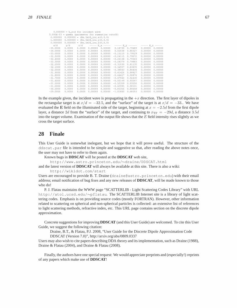
28 FINALE 67

0.000000 = k_z * d for incident wave5.000E-03 = gamma (parameter for summation cutoff)

0.000000 0.000000 = (Re,Im)E_inc,x(0,0,0)1.000000 0.000000 = (Re,Im)E_inc,y(0,0,0)0.000000 0.000000 = (Re,Im)E_inc,z(0,0,0)

x/d y/d z/d ----- E_x ----- ----- E_y ------ ----- E_z ------35.0000 0.0000 0.0000 0.00000 0.00000 0.18730 0.79489 0.0 0000 0.00000-34.0000 0.0000 0.0000 0.00000 0.00000 0.02038 0.80327 0.0 0000 0.00000-33.0000 0.0000 0.0000 0.00000 0.00000 -0.15115 0.79529 0. 00000 0.00000-32.5000 0.0000 0.0000 0.00000 0.00000 -0.24115 0.79072 0. 00000 0.00000-32.4000 0.0000 0.0000 0.00000 0.00000 -0.26138 0.79303 0. 00000 0.00000-32.3000 0.0000 0.0000 0.00000 0.00000 -0.28379 0.79883 0. 00000 0.00000-32.2000 0.0000 0.0000 0.00000 0.00000 -0.31030 0.81135 0. 00000 0.00000-32.1000 0.0000 0.0000 0.00000 0.00000 -0.34557 0.83835 0. 00000 0.00000-32.0000 0.0000 0.0000 0.00000 0.00000 -0.38043 0.86434 0. 00000 0.00000-31.9000 0.0000 0.0000 0.00000 0.00000 -0.41426 0.88827 0. 00000 0.00000-31.8000 0.0000 0.0000 0.00000 0.00000 -0.44627 0.90876 0. 00000 0.00000-31.7000 0.0000 0.0000 0.00000 0.00000 -0.47560 0.92430 0. 00000 0.00000-31.6000 0.0000 0.0000 0.00000 0.00000 -0.50149 0.93347 0. 00000 0.00000-31.5000 0.0000 0.0000 0.00000 0.00000 -0.52359 0.93550 0. 00000 0.00000-31.0000 0.0000 0.0000 0.00000 0.00000 -0.62995 0.90101 0. 00000 0.00000-30.0000 0.0000 0.0000 0.00000 0.00000 -0.83356 0.80658 0. 00000 0.00000-29.0000 0.0000 0.0000 0.00000 0.00000 -1.01850 0.68353 0. 00000 0.00000

In the example given, the incident wave is propagating in the+x direction. The first layer of dipoles inthe rectangular target is atx/d = −32.5, and the “surface” of the target is atx/d = −33.. We haveevaluated theE field on the illuminated side of the target, beginning atx = −2.5d from the first dipolelayer, a distance2d from the “surface” of the target, and continuing toxTF = −29d, a distance3.5dinto the target volume. Examination of the output file shows that theE field intensity rises slightly as wecross the target surface.

28 Finale

This User Guide is somewhat inelegant, but we hope that it will prove useful. The structure of theddscat.par file is intended to be simple and suggestive so that, after reading the above notes once,the user may not have to refer to them again.

Known bugs inDDSCAT will be posted at theDDSCAT web site,http://www.astro.princeton.edu/ ∼draine/DDSCAT.html

and the latest version ofDDSCAT will always be available at this site. There is also a wiki:http://wikidot.com/start

Users are encouraged to provide B. T. Draine (draine@astro.princeton.edu ) with their emailaddress; email notification of bug fixes and any new releases of DDSCAT, will be made known to thosewho do!

P. J. Flatau maintains the WWW page “SCATTERLIB - Light Scattering Codes Library” with URLhttp://atol.ucsd.edu/ ∼pflatau . The SCATTERLIB Internet site is a library of light scat-tering codes. Emphasis is on providing source codes (mostlyFORTRAN). However, other informationrelated to scattering on spherical and non-spherical particles is collected: an extensive list of referencesto light scattering methods, refractive index, etc. This URL page contains section on the discrete dipoleapproximation.

Concrete suggestions for improvingDDSCAT (and this User Guide) are welcomed. To cite this UserGuide, we suggest the following citation:

Draine, B.T., & Flatau, P.J. 2008, “User Guide for the Discrete Dipole Approximation CodeDDSCAT (Version 7.0)”, http://arxiv.org/abs/0809.0337

Users may also wish to cite papers describing DDA theory and its implementation, such as Draine (1988),Draine & Flatau (2004), and Draine & Flatau (2008).

Finally, the authors have one special request: We would appreciate preprints and (especially!) reprintsof any papers which make use ofDDSCAT!

29 ACKNOWLEDGMENTS 68

29 Acknowledgments

• The routineESELFmaking use of the FFT was originally written by Jeremy Goodman, PrincetonUniversity Observatory.

• The FFT routineFOURX, used in the comparison of different FFT routines, is based on a FFTroutine written by Norman Brenner (Brenner 1969).

• TheGPFAPACKpackage was written by Clive Temperton (1992), and generously made availableby him for use withDDSCAT.

• Much of the work involved in modifyingDDSCATto useMPI was done by Matthew Collinge,Princeton University.

• The conjugate gradient routineZBCG2was written by M.A. Botchev(http://www.math.utwente.nl/ ∼botchev/ ), based on earlier work by D.R. Fokkema(Dept. of Mathematics, Utrecht University).

• Art Lazanoff (NASA Ames Research Center) did most of the coding necessary to use OpenMPand to use theDFTI library routine from the IntelR© Math Kernel Library, as well as considerabletesting of the new code.

We are deeply indebted to all of these authors for making their work and code available.We wish also to acknowledge bug reports and suggestions fromDDSCAT users, including Stefan

Kniefl, Henrietta Lemke, Georges Levi, Wang Lin, Paul Mulvaney, Timo Nousianen, Stuart Prescott,and Mike Wolff.

Development ofDDSCAT was supported in part by National Science Foundation grantsAST-8341412,AST-8612013, AST-9017082, AST-9319283, AST-9616429, AST-9988126, AST-0406883 to BTD, inpart by support from the Office of Naval Research Young Investigator Program to PJF, in part by DuPontCorporate Educational Assistance to PJF, and in part by the United Kingdom Defence Research Agency.

References

[1] Bohren, C.F., and Huffman, D.R. 1983,Absorption and Scattering of Light by Small Particles(NewYork: Wiley-Interscience).

[2] Brenner, N.M. 1969,IEEE Trans. Audio Electroacoust.AU-17, 128.

[3] Collinge, M.J, and Draine, B.T. 2004, “Discrete dipole approximation with polarizabilitiesthat account for both finite wavelength and target geometry”, J. Opt. Soc. Am. A, in press.[http://arxiv.org/abs/astro-ph/0311304]

[4] Draine, B.T. 1988, “The Discrete-Dipole Approximationand Its Application to Interstellar GraphiteGrains”,Astrophysical J., 333, 848-872.

[5] Draine, B.T. 2000, “The Discrete-Dipole Approximationfor Light Scattering by Irregular Targets”,in Light Scattering by Nonspherical Particles: Theory, Measurements, and Geophysical Applications,ed. M.I. Mishchenko, J.W. Hovenier, and L.D. Travis (N.Y.: Academic Press), 131-145.

[6] Draine, B.T. 2003, “Scattering by Interstellar Grains.I. Optical and Ultraviolet”,Astrophysical J.,598, 1017-1025.

[7] Draine, B.T., and Flatau, P.J. 1994, “Discrete-dipole approximation for scattering calculations”,J.Opt. Soc. Am. A, 11, 1491-1499.

[8] Draine, B.T., and Flatau, P.J. 2008, this document: “User Guide for the Discrete Dipole Approxima-tion Code DDSCAT 7.0”, http://arxiv.org/abs/0809.0337.

[9] Draine, B.T., and Flatau, P.J. 2008, “The discrete dipole approximation for periodic targets: theoryand tests”, JOSA A,25, 2693-2703.

[10] Draine, B.T., and Goodman, J.J. 1993, “Beyond Clausius-Mossotti: Wave Propagation on a Polar-izable Point Lattice and the Discrete Dipole Approximation”, Astrophysical J., 405, 685-697.

REFERENCES 69

[11] Draine, B.T., and Weingartner, J.C. 1996, “Radiative Torques on Interstellar Grains: I. Superther-mal Rotation”,Astrophysical J., 470, 551-565.

[12] Draine, B.T., and Weingartner, J.C. 1997, “Radiative Torques on Interstellar Grains: II. Alignmentwith the Magnetic Field”,Astrophysical J., 480, 633-646.

[13] Flatau, P.J. 1997, “Improvements in the discrete dipole approximation method of computing scat-tering and absorption”,Optics Lett., 22, 1205-1207

[14] Flatau, P.J., Stephens, G.L., and Draine, B.T. 1990, “Light scattering by rectangular solids in thediscrete-dipole approximation: a new algorithm exploiting the Block-Toeplitz structure”,J. Opt. Soc.Am. A, 7, 593-600.

[15] Goedecke, G.H., and O’Brien, S.G. 1988, “Scattering byirregular inhomogeneous particles via thedigitized Green’s function algorithm”,Appl. Opt., 28, 2431-2438.

[16] Goodman, J.J., Draine, B.T., and Flatau, P.J. 1991, “Application of FFT Techniques to the DiscreteDipole Approximation,Opt. Lett., 16, 1198-1200.

[17] Gutkowicz-Krusin, D., & Draine, B.T. 2004, “Propagation of Electromagnetic Waves on a Rectan-gular Lattice of Polarizable Points”, http://arxiv.org/abs/astro-ph/0403082

[18] Hage, J.I., and Greenberg, J.M. 1990, “A Model for the Optical Properties of Porous Grains”,Astrophysical J., 361, 251-259.

[19] Petravic, M., & Kuo-Petravic, G. 1979, “An ILUCG algorithm which minimizes in the Euclideannorm”, J. Computational Phys., 32, 263-269.

[20] Purcell, E.M., and Pennypacker, C.R. 1973, “Scattering and Absorption of Light by NonsphericalDielectric Grains”, Astrophysical J.,186, 705-714.

[21] Sleijpen, G.L.G., & van der Vorst, H.A. 1995, “Maintaining convergence properties of BiCGstabmethods in finite precision arithmetic”,Numerical Algorithms, 10, 203-223.

[22] Sleijpen, G.L.G., & van der Vorst, H.A. 1996, “Reliableupdated residuals in hybrid Bi-CG meth-ods”,Computing, 56, 141-163.

[23] Temperton, C.J. 1983, “Self-sorting mixed-radix FastFourier Transforms”,J. Comp. Phys., 52,1-23.

[24] Temperton, C. 1992, “A Generalized Prime Factor FFT Algorithm for Any N = 2p3q5r”, SIAMJournal of Scientific and Statistical Computing, 13, 676-686

A UNDERSTANDING AND MODIFYING DDSCAT.PAR 70

A Understanding and Modifying ddscat.par

In order to use DDSCAT to perform the specific calculations ofinterest to you, it will be necessary tomodify theddscat.par file. Here we list the sampleddscat.par file, followed by a discussion ofhow to modify this file as needed. Note that all numerical input data in DDSCAT is read with free-formatREAD(IDEV, * )... statements. Therefore you do not need to worry about the precise format in whichinteger or floating point numbers are entered on a line. The crucial thing is that lines inddscat.parcontaining numerical data have the correct number of data entries, with any informational commentsappearingafter the numerical data on a given line.

’ ========= Parameter file for v7.0.7 =================== ’’ **** Preliminaries **** ’’NOTORQ’ = CMTORQ* 6 (NOTORQ, DOTORQ) -- either do or skip torque calculations’PBCGS2’ = CMDSOL* 6 (PBCGS2, PBCGST, PETRKP) -- select solution method’GPFAFT’ = CMDFFT* 6 (GPFAFT, FFTMKL)’GKDLDR’ = CALPHA* 6 (GKDLDR, LATTDR’NOTBIN’ = CBINFLAG (NOTBIN, ORIBIN, ALLBIN)’ **** Initial Memory Allocation **** ’100 100 100 = dimensioning allowance for target generation’ **** Target Geometry and Composition **** ’’RCTGLPRSM’ = CSHAPE* 9 shape directive32 24 16 = shape parameters 1 - 31 = NCOMP = number of dielectric materials’diel.tab’ = file with refractive index 1’ **** Error Tolerance **** ’1.00e-5 = TOL = MAX ALLOWED (NORM OF |G>=AC|E>-ACA|X>)/(NORM OF AC|E>)’ **** Interaction cutoff parameter for PBC calculations **** ’5.00e-3 = GAMMA (1e-2 is normal, 3e-3 for greater accuracy)’ **** Angular resolution for calculation of <cos>, etc. **** ’0.5 = ETASCA (number of angles is proportional to [(3+x)/ETA SCA]ˆ2 )’ **** Wavelengths (micron) **** ’6.283185 6.283185 1 ’LIN’ = wavelengths (first,last,how ma ny,how=LIN,INV,LOG)’ **** Effective Radii (micron) **** ’2 2 1 ’LIN’ = aeff (first,last,how many,how=LIN,INV,LOG)’ **** Define Incident Polarizations **** ’(0,0) (1.,0.) (0.,0.) = Polarization state e01 (k along x axi s)2 = IORTH (=1 to do only pol. state e01; =2 to also do orth. pol. s tate)’ **** Specify which output files to write **** ’1 = IWRKSC (=0 to suppress, =1 to write ".sca" file for each tar get orient.1 = IWRPOL (=0 to suppress, =1 to write ".pol" file for each (BE TA,THETA)’ **** Prescribe Target Rotations **** ’0. 0. 1 = BETAMI, BETAMX, NBETA (beta=rotation around a1)0. 90. 3 = THETMI, THETMX, NTHETA (theta=angle between a1 and k)0. 0. 1 = PHIMIN, PHIMAX, NPHI (phi=rotation angle of a1 aroun d k)’ **** Specify first IWAV, IRAD, IORI (normally 0 0 0) **** ’0 0 0 = first IWAV, first IRAD, first IORI (0 0 0 to begin fresh)’ **** Select Elements of S_ij Matrix to Print **** ’6 = NSMELTS = number of elements of S_ij to print (not more than 9)11 12 21 22 31 41 = indices ij of elements to print’ **** Specify Scattered Directions **** ’’LFRAME’ = CMDFRM (LFRAME, TFRAME for Lab Frame or Target Fra me)2 = NPLANES = number of scattering planes0. 0. 180. 10 = phi, thetan_min, thetan_max, dtheta (in deg) f or plane 190. 0. 180. 10 = phi, thetan_min, thetan_max, dtheta (in deg) for plane 2

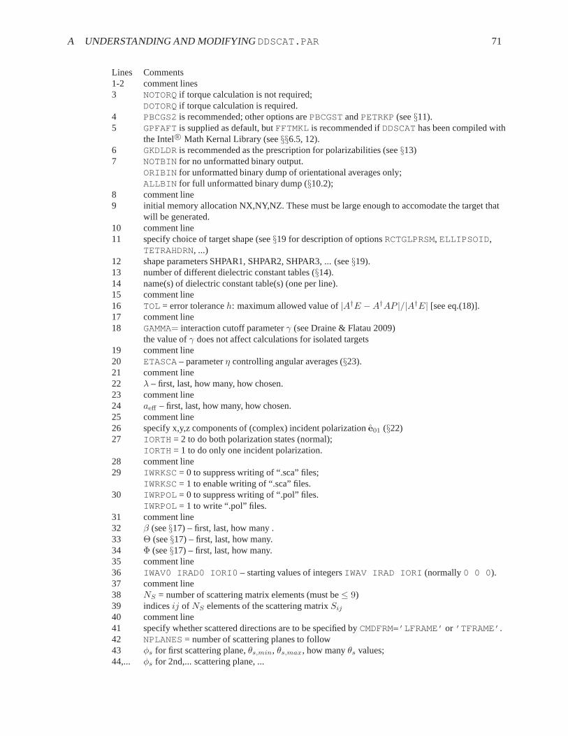
A UNDERSTANDING AND MODIFYING DDSCAT.PAR 71

Lines Comments1-2 comment lines3 NOTORQif torque calculation is not required;

DOTORQif torque calculation is required.4 PBCGS2is recommended; other options arePBCGSTandPETRKP(see§11).5 GPFAFTis supplied as default, butFFTMKLis recommended ifDDSCAThas been compiled with

the IntelR© Math Kernal Library (see§§6.5, 12).6 GKDLDRis recommended as the prescription for polarizabilities (see§13)7 NOTBINfor no unformatted binary output.

ORIBIN for unformatted binary dump of orientational averages only;ALLBIN for full unformatted binary dump (§10.2);

8 comment line9 initial memory allocation NX,NY,NZ. These must be large enough to accomodate the target that

will be generated.10 comment line11 specify choice of target shape (see§19 for description of optionsRCTGLPRSM, ELLIPSOID ,

TETRAHDRN, ...)12 shape parameters SHPAR1, SHPAR2, SHPAR3, ... (see§19).13 number of different dielectric constant tables (§14).14 name(s) of dielectric constant table(s) (one per line).15 comment line16 TOL= error toleranceh: maximum allowed value of|A†E − A†AP |/|A†E| [see eq.(18)].17 comment line18 GAMMA= interaction cutoff parameterγ (see Draine & Flatau 2009)

the value ofγ does not affect calculations for isolated targets19 comment line20 ETASCA– parameterη controlling angular averages (§23).21 comment line22 λ – first, last, how many, how chosen.23 comment line24 aeff – first, last, how many, how chosen.25 comment line26 specify x,y,z components of (complex) incident polarization e01 (§22)27 IORTH= 2 to do both polarization states (normal);

IORTH= 1 to do only one incident polarization.28 comment line29 IWRKSC= 0 to suppress writing of “.sca” files;

IWRKSC= 1 to enable writing of “.sca” files.30 IWRPOL= 0 to suppress writing of “.pol” files.

IWRPOL= 1 to write “.pol” files.31 comment line32 β (see§17) – first, last, how many .33 Θ (see§17) – first, last, how many.34 Φ (see§17) – first, last, how many.35 comment line36 IWAV0 IRAD0 IORI0 – starting values of integersIWAV IRAD IORI (normally0 0 0 ).37 comment line38 NS = number of scattering matrix elements (must be≤ 9)39 indicesij of NS elements of the scattering matrixSij

40 comment line41 specify whether scattered directions are to be specified by CMDFRM=’LFRAME’or ’TFRAME’ .42 NPLANES= number of scattering planes to follow43 φs for first scattering plane,θs,min, θs,max, how manyθs values;44,... φs for 2nd,... scattering plane, ...

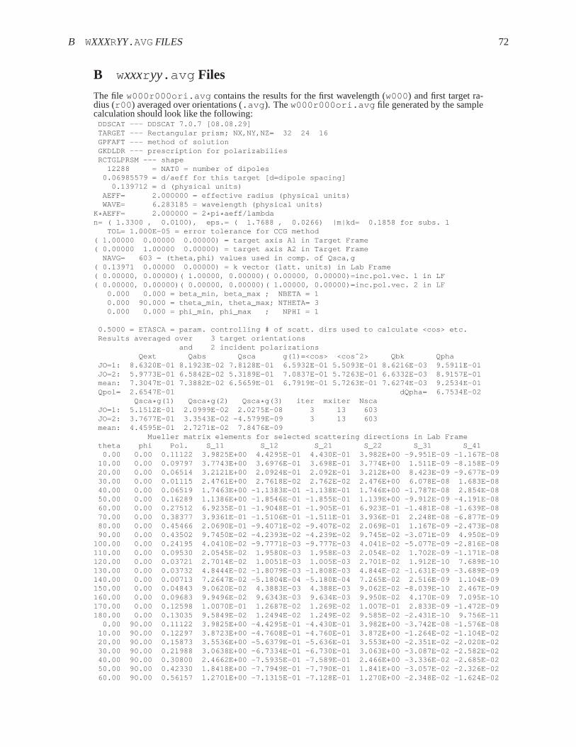
B WXXXRYY.AVG FILES 72

B wxxxr yy.avg Files

The file w000r000ori.avg contains the results for the first wavelength (w000) and first target ra-dius (r00 ) averaged over orientations (.avg ). Thew000r000ori.avg file generated by the samplecalculation should look like the following:

DDSCAT --- DDSCAT 7.0.7 [08.08.29]TARGET --- Rectangular prism; NX,NY,NZ= 32 24 16GPFAFT --- method of solutionGKDLDR --- prescription for polarizabiliesRCTGLPRSM --- shape

12288 = NAT0 = number of dipoles0.06985579 = d/aeff for this target [d=dipole spacing]

0.139712 = d (physical units)AEFF= 2.000000 = effective radius (physical units)WAVE= 6.283185 = wavelength (physical units)

K* AEFF= 2.000000 = 2 * pi * aeff/lambdan= ( 1.3300 , 0.0100), eps.= ( 1.7688 , 0.0266) |m|kd= 0.1858 f or subs. 1

TOL= 1.000E-05 = error tolerance for CCG method( 1.00000 0.00000 0.00000) = target axis A1 in Target Frame( 0.00000 1.00000 0.00000) = target axis A2 in Target Frame

NAVG= 603 = (theta,phi) values used in comp. of Qsca,g( 0.13971 0.00000 0.00000) = k vector (latt. units) in Lab Fra me( 0.00000, 0.00000)( 1.00000, 0.00000)( 0.00000, 0.00000) =inc.pol.vec. 1 in LF( 0.00000, 0.00000)( 0.00000, 0.00000)( 1.00000, 0.00000) =inc.pol.vec. 2 in LF

0.000 0.000 = beta_min, beta_max ; NBETA = 10.000 90.000 = theta_min, theta_max; NTHETA= 30.000 0.000 = phi_min, phi_max ; NPHI = 1

0.5000 = ETASCA = param. controlling # of scatt. dirs used to c alculate <cos> etc.Results averaged over 3 target orientations

and 2 incident polarizationsQext Qabs Qsca g(1)=<cos> <cosˆ2> Qbk Qpha

JO=1: 8.6320E-01 8.1923E-02 7.8128E-01 6.5932E-01 5.5093 E-01 8.6216E-03 9.5911E-01JO=2: 5.9773E-01 6.5842E-02 5.3189E-01 7.0837E-01 5.7263 E-01 6.6332E-03 8.9157E-01mean: 7.3047E-01 7.3882E-02 6.5659E-01 6.7919E-01 5.7263 E-01 7.6274E-03 9.2534E-01Qpol= 2.6547E-01 dQpha= 6.7534E-02

Qsca* g(1) Qsca * g(2) Qsca * g(3) iter mxiter NscaJO=1: 5.1512E-01 2.0999E-02 2.0275E-08 3 13 603JO=2: 3.7677E-01 3.3543E-02 -4.5799E-09 3 13 603mean: 4.4595E-01 2.7271E-02 7.8476E-09

Mueller matrix elements for selected scattering direction s in Lab Frametheta phi Pol. S_11 S_12 S_21 S_22 S_31 S_41

0.00 0.00 0.11122 3.9825E+00 4.4295E-01 4.430E-01 3.982E+ 00 -9.951E-09 -1.167E-0810.00 0.00 0.09797 3.7743E+00 3.6976E-01 3.698E-01 3.774E +00 1.511E-09 -8.158E-0920.00 0.00 0.06514 3.2121E+00 2.0924E-01 2.092E-01 3.212E +00 8.423E-09 -9.677E-0930.00 0.00 0.01115 2.4761E+00 2.7618E-02 2.762E-02 2.476E +00 6.078E-08 1.683E-0840.00 0.00 0.06519 1.7463E+00 -1.1383E-01 -1.138E-01 1.74 6E+00 -1.787E-08 2.854E-0850.00 0.00 0.16289 1.1386E+00 -1.8546E-01 -1.855E-01 1.13 9E+00 -9.912E-09 -4.191E-0860.00 0.00 0.27512 6.9235E-01 -1.9048E-01 -1.905E-01 6.92 3E-01 -1.481E-08 -1.639E-0870.00 0.00 0.38377 3.9361E-01 -1.5106E-01 -1.511E-01 3.93 6E-01 2.248E-08 -6.877E-0980.00 0.00 0.45466 2.0690E-01 -9.4071E-02 -9.407E-02 2.06 9E-01 1.167E-09 -2.473E-0890.00 0.00 0.43502 9.7450E-02 -4.2393E-02 -4.239E-02 9.74 5E-02 -3.071E-09 4.950E-09

100.00 0.00 0.24195 4.0410E-02 -9.7771E-03 -9.777E-03 4.0 41E-02 -5.077E-09 -2.816E-08110.00 0.00 0.09530 2.0545E-02 1.9580E-03 1.958E-03 2.054 E-02 1.702E-09 -1.171E-08120.00 0.00 0.03721 2.7014E-02 1.0051E-03 1.005E-03 2.701 E-02 1.912E-10 7.689E-10130.00 0.00 0.03732 4.8444E-02 -1.8079E-03 -1.808E-03 4.8 44E-02 -1.631E-09 -3.689E-09140.00 0.00 0.00713 7.2647E-02 -5.1804E-04 -5.180E-04 7.2 65E-02 2.516E-09 1.104E-09150.00 0.00 0.04843 9.0620E-02 4.3883E-03 4.388E-03 9.062 E-02 -8.039E-10 2.467E-09160.00 0.00 0.09683 9.9496E-02 9.6343E-03 9.634E-03 9.950 E-02 4.170E-09 7.095E-10170.00 0.00 0.12598 1.0070E-01 1.2687E-02 1.269E-02 1.007 E-01 2.833E-09 -1.472E-09180.00 0.00 0.13035 9.5849E-02 1.2494E-02 1.249E-02 9.585 E-02 -2.431E-10 9.756E-11

0.00 90.00 0.11122 3.9825E+00 -4.4295E-01 -4.430E-01 3.98 2E+00 -3.742E-08 -1.576E-0810.00 90.00 0.12297 3.8723E+00 -4.7608E-01 -4.760E-01 3.8 72E+00 -1.264E-02 -1.104E-0220.00 90.00 0.15873 3.5536E+00 -5.6379E-01 -5.636E-01 3.5 53E+00 -2.351E-02 -2.020E-0230.00 90.00 0.21988 3.0638E+00 -6.7334E-01 -6.730E-01 3.0 63E+00 -3.087E-02 -2.582E-0240.00 90.00 0.30800 2.4662E+00 -7.5935E-01 -7.589E-01 2.4 66E+00 -3.336E-02 -2.685E-0250.00 90.00 0.42330 1.8418E+00 -7.7949E-01 -7.790E-01 1.8 41E+00 -3.057E-02 -2.326E-0260.00 90.00 0.56157 1.2701E+00 -7.1315E-01 -7.128E-01 1.2 70E+00 -2.348E-02 -1.624E-02

B WXXXRYY.AVG FILES 73

70.00 90.00 0.71013 8.0650E-01 -5.7261E-01 -5.725E-01 8.0 62E-01 -1.433E-02 -7.917E-0380.00 90.00 0.84528 4.7037E-01 -3.9748E-01 -3.975E-01 4.7 02E-01 -5.730E-03 -5.546E-0490.00 90.00 0.93786 2.5001E-01 -2.3444E-01 -2.345E-01 2.4 98E-01 3.705E-04 4.290E-03

100.00 90.00 0.96898 1.1900E-01 -1.1547E-01 -1.153E-01 1. 186E-01 3.258E-03 6.211E-03110.00 90.00 0.93364 5.0906E-02 -4.7946E-02 -4.740E-02 5. 024E-02 3.410E-03 5.818E-03120.00 90.00 0.76404 2.5253E-02 -1.9997E-02 -1.919E-02 2. 437E-02 1.966E-03 4.206E-03130.00 90.00 0.47038 2.6571E-02 -1.3386E-02 -1.250E-02 2. 563E-02 1.256E-04 2.390E-03140.00 90.00 0.31141 4.2301E-02 -1.3889E-02 -1.311E-02 4. 150E-02 -1.273E-03 9.800E-04150.00 90.00 0.22711 6.2453E-02 -1.4597E-02 -1.406E-02 6. 190E-02 -1.874E-03 1.589E-04160.00 90.00 0.17277 8.0205E-02 -1.4023E-02 -1.375E-02 7. 993E-02 -1.704E-03 -1.593E-04170.00 90.00 0.14092 9.1846E-02 -1.2978E-02 -1.290E-02 9. 177E-02 -9.878E-04 -1.543E-04180.00 90.00 0.13035 9.5849E-02 -1.2494E-02 -1.249E-02 9. 585E-02 1.420E-09 4.482E-10

C WXXXRYYYKZZZ.SCA FILES 74

C wxxxr yyykzzz.sca Files

Thew000r000k000.sca file contains the results for the first wavelength (w000), first target radius(r00 ), and first orientation (k000 ). Thew000r000k000.sca file created by the sample calculationshould look like the following:

DDSCAT --- DDSCAT 7.0.7 [08.08.29]TARGET --- Rectangular prism; NX,NY,NZ= 32 24 16GPFAFT --- method of solutionGKDLDR --- prescription for polarizabiliesRCTGLPRSM --- shape

12288 = NAT0 = number of dipoles0.06985579 = d/aeff for this target [d=dipole spacing]

0.139712 = d (physical units)----- physical extent of target volume in Target Frame ----- -

-4.470771 0.000000 = xmin,xmax (physical units)-1.676539 1.676539 = ymin,ymax (physical units)-1.117693 1.117693 = zmin,zmax (physical units)

AEFF= 2.000000 = effective radius (physical units)WAVE= 6.283185 = wavelength (physical units)

K* AEFF= 2.000000 = 2 * pi * aeff/lambdan= ( 1.3300 , 0.0100), eps.= ( 1.7688 , 0.0266) |m|kd= 0.1858 f or subs. 1

TOL= 1.000E-05 = error tolerance for CCG method( 1.00000 0.00000 0.00000) = target axis A1 in Target Frame( 0.00000 1.00000 0.00000) = target axis A2 in Target Frame

NAVG= 603 = (theta,phi) values used in comp. of Qsca,g( 0.13971 0.00000 0.00000) = k vector (latt. units) in TF( 0.00000, 0.00000)( 1.00000, 0.00000)( 0.00000, 0.00000) =inc.pol.vec. 1 in TF( 0.00000, 0.00000)( 0.00000, 0.00000)( 1.00000, 0.00000) =inc.pol.vec. 2 in TF( 1.00000 0.00000 0.00000) = target axis A1 in Lab Frame( 0.00000 1.00000 0.00000) = target axis A2 in Lab Frame( 0.13971 0.00000 0.00000) = k vector (latt. units) in Lab Fra me( 0.00000, 0.00000)( 1.00000, 0.00000)( 0.00000, 0.00000) =inc.pol.vec. 1 in LF( 0.00000, 0.00000)( 0.00000, 0.00000)( 1.00000, 0.00000) =inc.pol.vec. 2 in LF

BETA = 0.000 = rotation of target around A1THETA= 0.000 = angle between A1 and k

PHI = 0.000 = rotation of A1 around k0.5000 = ETASCA = param. controlling # of scatt. dirs used to c alculate <cos> etc.

Qext Qabs Qsca g(1)=<cos> <cosˆ2> Qbk QphaJO=1: 9.0997E-01 8.6105E-02 8.2387E-01 6.4090E-01 5.8427 E-01 2.5108E-02 9.7717E-01JO=2: 6.9891E-01 7.0519E-02 6.2839E-01 6.5894E-01 6.0509 E-01 1.9097E-02 9.1277E-01mean: 8.0444E-01 7.8312E-02 7.2613E-01 6.4871E-01 5.9328 E-01 2.2103E-02 9.4497E-01Qpol= 2.1106E-01 dQpha= 6.4397E-02

Qsca* g(1) Qsca * g(2) Qsca * g(3) iter mxiter NscaJO=1: 5.2802E-01 -1.2657E-08 -1.6907E-08 3 13 603JO=2: 4.1407E-01 -4.0495E-08 -1.0475E-09 3 13 603mean: 4.7105E-01 -2.6576E-08 -8.9774E-09

Mueller matrix elements for selected scattering direction s in Lab Frametheta phi Pol. S_11 S_12 S_21 S_22 S_31 S_41

0.00 0.00 0.09758 4.2343E+00 4.1320E-01 4.132E-01 4.234E+ 00 3.953E-10 1.753E-1010.00 0.00 0.08802 4.0521E+00 3.5667E-01 3.567E-01 4.052E +00 1.105E-08 -2.338E-0820.00 0.00 0.05875 3.5445E+00 2.0822E-01 2.082E-01 3.544E +00 -1.771E-08 -3.568E-0830.00 0.00 0.00810 2.8187E+00 2.2829E-02 2.283E-02 2.819E +00 3.923E-08 -1.997E-0840.00 0.00 0.06619 2.0233E+00 -1.3391E-01 -1.339E-01 2.02 3E+00 -6.927E-08 1.304E-0750.00 0.00 0.16569 1.3011E+00 -2.1558E-01 -2.156E-01 1.30 1E+00 -1.984E-08 -2.180E-0860.00 0.00 0.28746 7.4420E-01 -2.1393E-01 -2.139E-01 7.44 2E-01 -5.892E-08 -1.007E-0770.00 0.00 0.41470 3.7493E-01 -1.5549E-01 -1.555E-01 3.74 9E-01 6.340E-08 4.262E-0880.00 0.00 0.49576 1.6262E-01 -8.0621E-02 -8.062E-02 1.62 6E-01 6.664E-09 -3.151E-0890.00 0.00 0.38933 5.6897E-02 -2.2152E-02 -2.215E-02 5.69 0E-02 -1.247E-08 -1.200E-08

100.00 0.00 0.34694 1.4850E-02 5.1520E-03 5.152E-03 1.485 E-02 -3.687E-09 -8.223E-10110.00 0.00 0.39736 1.1368E-02 4.5172E-03 4.517E-03 1.137 E-02 6.363E-09 -1.163E-09120.00 0.00 0.25849 3.5576E-02 -9.1961E-03 -9.196E-03 3.5 58E-02 5.643E-09 1.226E-09130.00 0.00 0.23722 8.1132E-02 -1.9246E-02 -1.925E-02 8.1 13E-02 3.549E-09 1.945E-09140.00 0.00 0.11691 1.3870E-01 -1.6215E-02 -1.621E-02 1.3 87E-01 1.278E-09 -6.238E-09150.00 0.00 0.00662 1.9560E-01 -1.2942E-03 -1.294E-03 1.9 56E-01 -4.405E-09 3.582E-10160.00 0.00 0.07326 2.4079E-01 1.7640E-02 1.764E-02 2.408 E-01 -4.924E-09 3.527E-09170.00 0.00 0.12045 2.6855E-01 3.2348E-02 3.235E-02 2.686 E-01 8.082E-10 -4.232E-09180.00 0.00 0.13599 2.7775E-01 3.7772E-02 3.777E-02 2.778 E-01 -1.008E-09 1.213E-10

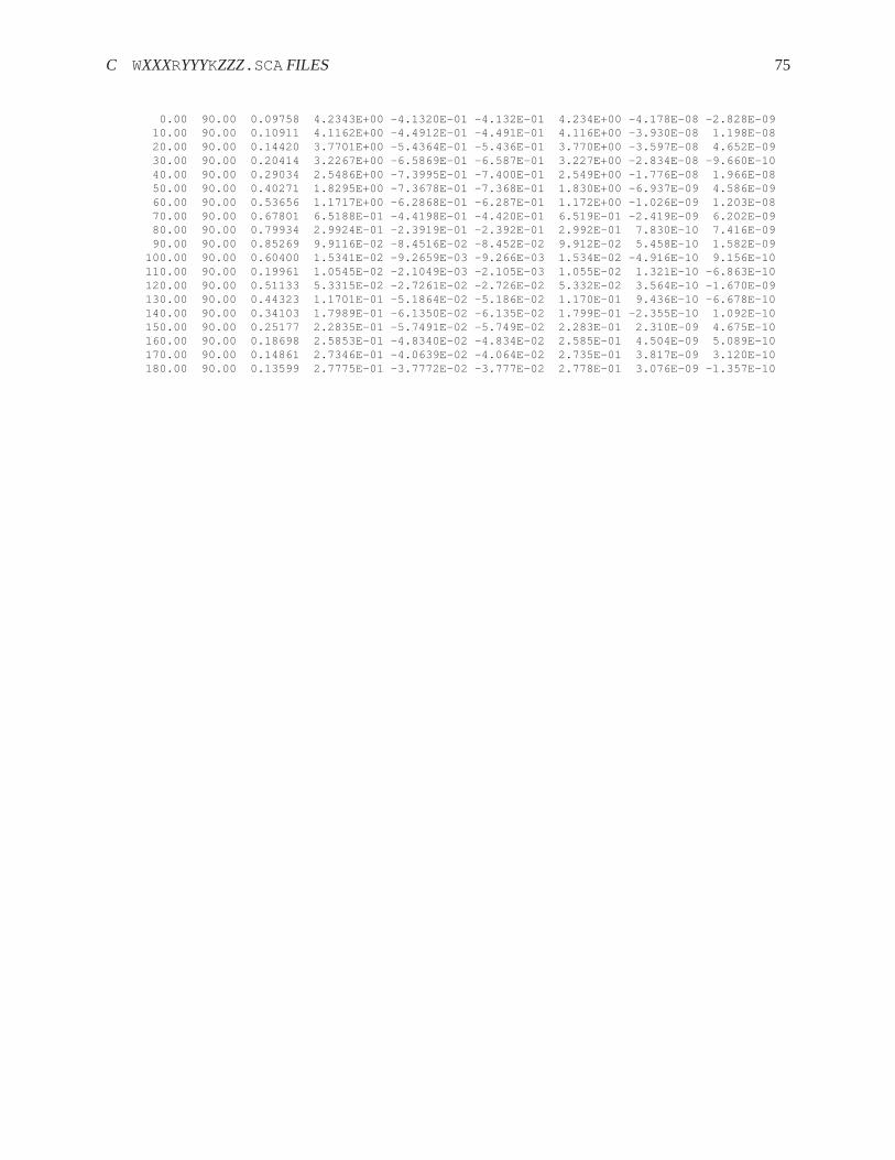
C WXXXRYYYKZZZ.SCA FILES 75

0.00 90.00 0.09758 4.2343E+00 -4.1320E-01 -4.132E-01 4.23 4E+00 -4.178E-08 -2.828E-0910.00 90.00 0.10911 4.1162E+00 -4.4912E-01 -4.491E-01 4.1 16E+00 -3.930E-08 1.198E-0820.00 90.00 0.14420 3.7701E+00 -5.4364E-01 -5.436E-01 3.7 70E+00 -3.597E-08 4.652E-0930.00 90.00 0.20414 3.2267E+00 -6.5869E-01 -6.587E-01 3.2 27E+00 -2.834E-08 -9.660E-1040.00 90.00 0.29034 2.5486E+00 -7.3995E-01 -7.400E-01 2.5 49E+00 -1.776E-08 1.966E-0850.00 90.00 0.40271 1.8295E+00 -7.3678E-01 -7.368E-01 1.8 30E+00 -6.937E-09 4.586E-0960.00 90.00 0.53656 1.1717E+00 -6.2868E-01 -6.287E-01 1.1 72E+00 -1.026E-09 1.203E-0870.00 90.00 0.67801 6.5188E-01 -4.4198E-01 -4.420E-01 6.5 19E-01 -2.419E-09 6.202E-0980.00 90.00 0.79934 2.9924E-01 -2.3919E-01 -2.392E-01 2.9 92E-01 7.830E-10 7.416E-0990.00 90.00 0.85269 9.9116E-02 -8.4516E-02 -8.452E-02 9.9 12E-02 5.458E-10 1.582E-09

100.00 90.00 0.60400 1.5341E-02 -9.2659E-03 -9.266E-03 1. 534E-02 -4.916E-10 9.156E-10110.00 90.00 0.19961 1.0545E-02 -2.1049E-03 -2.105E-03 1. 055E-02 1.321E-10 -6.863E-10120.00 90.00 0.51133 5.3315E-02 -2.7261E-02 -2.726E-02 5. 332E-02 3.564E-10 -1.670E-09130.00 90.00 0.44323 1.1701E-01 -5.1864E-02 -5.186E-02 1. 170E-01 9.436E-10 -6.678E-10140.00 90.00 0.34103 1.7989E-01 -6.1350E-02 -6.135E-02 1. 799E-01 -2.355E-10 1.092E-10150.00 90.00 0.25177 2.2835E-01 -5.7491E-02 -5.749E-02 2. 283E-01 2.310E-09 4.675E-10160.00 90.00 0.18698 2.5853E-01 -4.8340E-02 -4.834E-02 2. 585E-01 4.504E-09 5.089E-10170.00 90.00 0.14861 2.7346E-01 -4.0639E-02 -4.064E-02 2. 735E-01 3.817E-09 3.120E-10180.00 90.00 0.13599 2.7775E-01 -3.7772E-02 -3.777E-02 2. 778E-01 3.076E-09 -1.357E-10

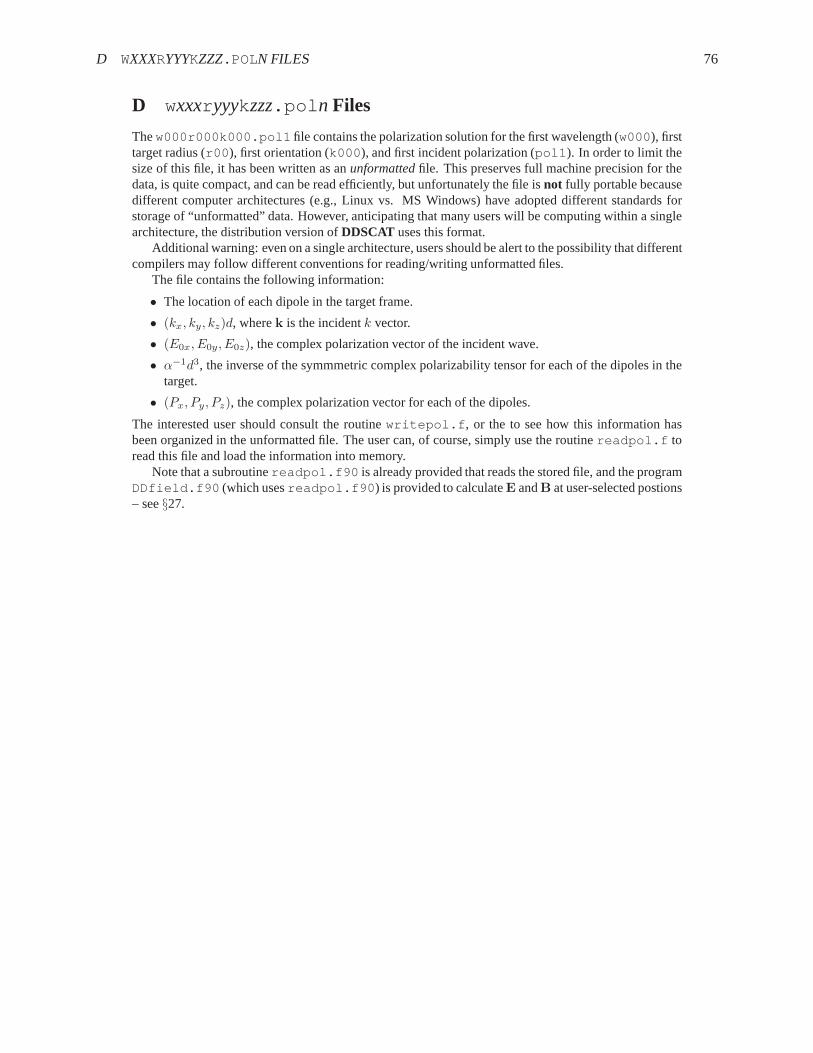
D WXXXRYYYKZZZ.POLNFILES 76

D wxxxr yyykzzz.pol n Files

Thew000r000k000.pol1 file contains the polarization solution for the first wavelength (w000), firsttarget radius (r00 ), first orientation (k000 ), and first incident polarization (pol1 ). In order to limit thesize of this file, it has been written as anunformattedfile. This preserves full machine precision for thedata, is quite compact, and can be read efficiently, but unfortunately the file isnot fully portable becausedifferent computer architectures (e.g., Linux vs. MS Windows) have adopted different standards forstorage of “unformatted” data. However, anticipating thatmany users will be computing within a singlearchitecture, the distribution version ofDDSCAT uses this format.

Additional warning: even on a single architecture, users should be alert to the possibility that differentcompilers may follow different conventions for reading/writing unformatted files.

The file contains the following information:

• The location of each dipole in the target frame.

• (kx, ky, kz)d, wherek is the incidentk vector.

• (E0x, E0y, E0z), the complex polarization vector of the incident wave.

• α−1d3, the inverse of the symmmetric complex polarizability tensor for each of the dipoles in thetarget.

• (Px, Py, Pz), the complex polarization vector for each of the dipoles.

The interested user should consult the routinewritepol.f , or the to see how this information hasbeen organized in the unformatted file. The user can, of course, simply use the routinereadpol.f toread this file and load the information into memory.

Note that a subroutinereadpol.f90 is already provided that reads the stored file, and the programDDfield.f90 (which usesreadpol.f90 ) is provided to calculateE andB at user-selected postions– see§27.

Index

Qabs, 8Qext, 8Qsca, 8Qpha, 8Sj – scattering amplitude matrix, 59Sij – 4×4 Mueller scattering matrix, 59, 60, 62Sj – scattering amplitude matrix, 60Φ – target orientation angle, 20, 30ΦDF, 40, 64Θ – target orientation angle, 20, 30ΘDF, 40, 64β – target orientation angle, 20, 30βDF, 40, 64η – parameter for choosing scattering angles, 59η – parameter for selection of scattering angles, 57a1, a2 target vectors, 20φs – scattering angle, 52, 57θs – scattering angle, 52, 57aeff , 7, 20fij – amplitude scattering matrix, 59fij – scattering amplitude matrix, 60QΓ – radiative torque efficiency vector, 28Qpr – radiative force efficiency vector, 28

absorption efficiency factorQabs, 8averages over scattering angles, 56

CALLTARGET, 41CALLTARGET and PBC, 42CMDFFT – specifying FFT method, 70CMDFRM – specifying scattering directions, 52, 70compiling and linking, 14conjugate gradient algorithm, 24Cygwin, 14, 18

DDfield, 20, 65ddscat.log000 – output file, 23ddscat.out, 23ddscat.par

ALLBIN, 24CSHAPE, 32diel.tab, 19DOTORQ, 28ETASCA, 28GAMMA, 19GKDLDR, 19, 26GPFAFT, 19IORTH, 59, 63IWRKSC, 23LATTDR, 19, 26NOTBIN, 19ORIBIN, 24

PBCGST, 24PETRKP, 24SHPAR1,SHPAR2,..., 32TOL, 24

ddscat.par – BETAMI,BETAMX,NBETA, 31ddscat.par – PHIMIN,PHIMAX,NPHI, 31ddscat.par – THETMI,THETMX,NTHETA, 31ddscat.par parameter file, 18diel.tab – see ddscat.par, 19Dielectric Frame (DF), 34, 40, 64dielectric function of target material, 26dielectric medium, 11dielectric tensor, 64differential scattering cross sectiondCsca/dΩ, 62DOTORQ, 28

effective radiusaeff , 7, 20Electric field in or near the target, 65ELLIPSOID, 37error tolerance, 24ESELF, 68ETASCA, 28extinction efficiency factorQext, 8

FFT algorithm, 25FFTW, 25Fortran compiler

optimization, 15

GAMMA – see ddscat.par, 19GKDLDR, 26GKDLDR – see ddscat.par, 19GPFA, 25GPFAFT, 47GPFAFT – see ddscat.par, 19GPFAPACK, 68

IDVERR, 16IDVOUT, 16infinite cylinder, 43infinite hexagonal column, 47IORTH, 63IORTH parameter, 59iterative algorithm, 24IWRKSC – see ddscat.par, 23IWRPOL, 65

Lab Frame (LF), 29LATTDR, 26LATTDR – see ddscat.par, 19LFRAME, 52

77

INDEX 78

Magnetic field in or near the target, 65memory requirements, 28MKL

Intel R© MKLDFTI, 15

MPI – Message Passing Interface, 16code execution, 22

MS-Windows and other abominations, 17mtable – output file, 23Mueller matrix for infinite targets, periodic in 1-d, 63Mueller matrix for infinite targets, periodic in 2-d, 63Mueller matrix for scattering, 59, 60, 62MXNX,MXNY,MXNZ, 28

NCOMPddscat.par, 19

NOTBIN – see ddscat.par, 19

orientational averaging, 31nonrandomly-oriented targets, 32randomly-oriented targets, 32

orientational sampling inβ, Θ, andΦ, 31

PBC = periodic boundary conditions, 54PBCGST algorithm, 24periodic boundary conditions, 36, 42, 44–47, 49–51PETRKP algorithm, 24phase lag efficiency factorQpha, 8PIM package, 24polarizabilities

GKDLDR, 26LATTDR, 26

polarization – elliptical, 59polarization of incident radiation, 55polarization of scattered radiation, 61, 62precision: single vs. double, 15PYD, 42, 46, 53, 54PZD, 42, 46, 54

qtable – output file, 23qtable2 – output file, 23qtable2 file, 23

radiative force efficiency vectorQpr, 28radiative torque efficiency vectorQΓ, 28READPOL, 65refractive index of target material, 26relative dielectric function, 11relative refractive index, 11

scattering – angular averages, 56scattering anglesθs, φs, 57scattering by tilted cube, 56scattering directions, 52scattering efficiency factorQsca, 8

SCATTERLIB, 67size parameterx = kaeff , 7source code (downloading of), 13Stokes vector(I, Q, U, V ), 60

Target Frame, 64Target Frame (TF), 30target generation, 32target generation: infinite periodic targets, 42target orientation, 29, 30target routines: modifying, 41target shape options

ANI ELL 2, 34ANI ELL 3, 34ANIELLIPS, 34ANIFRMFIL, 33ANIRCTNGL, 35BISLINPBC, 42CONELLIPS, 36CYLINDER1, 36CYLNDRCAP, 36CYLNDRPBC, 42DSKBLYPBC, 44DSKRCTNGL, 36DSKRCTPBC, 45DW1996TAR, 37ELLIPSO 2, 37ELLIPSO 3, 37ELLIPSOID, 37FROM FILE, 33HEX PRISM, 38HEXGONPBC, 46LAYRDSLAB, 38LYRSLBPBC, 47MLTBLOCKS, 38RCTGL PBC, 49RCTGLPRSM, 38RECRECPBC, 50SPH ANI N, 40SPHERESN, 39SPHRNPBC, 51SPHROID2, 40TETRAHDRN, 41TRILYRPBC, 52TRNGLPRSM, 41UNIAXICYL, 41

target shape optionszRCTGLBLK3, 39

target.out – output file, 42TFRAME, 52

w000r000k000.poln– output file, 23w000r000k000.sca – output file, 23w000r000ori.avg – output file, 23

INDEX 79

w000r000ori.avg file – output file, 23winzip, 14