DEGREE PROGRAMME IN WIRELESS COMMUNICATIONS ENGINEERING

MASTER’S THESIS

FASTER THAN NYQUIST SIGNALING AND ANALYSIS

OF ITS PERFORMANCE UNDER UNCODED/CODED

TRANSMISSION SYSTEMS

Author Ishwor Hadkhale

Supervisor Prof. Nandana Rajatheva

Second Examiner Dr. Pekka Pirinen

March, 2015

Hadkhale I. (2015) Faster than Nyquist Signaling and Analysis of its PerformanceUnder Uncoded/Coded Transmissions Systems. University of Oulu, Department ofCommunications Engineering, Degree Programme in Wireless Communications En-gineering. Master’s Thesis, 68p.

ABSTRACT

The future demand of increased transmission rate and bandwidth efficiency isof prime concern in the modern wireless communication systems. Faster thanNyquist signaling (FTN) is under the great interest of research to address thisissue of high data rate, which is also a major requirement, for the fifth generation(5G) communication networks.

The data bits are transmitted at a rate higher than the conventional methodswhich are bounded by the Nyquist condition and the outputs are compared soas to analyze the benefits. Receiver processing techniques are implemented toachieve the high data rate with improved error performance at the lower decodingcomplexity.

Considering the bandwidth efficiency as a key factor, more data symbols aresent at the given time interval by reducing the time period for signal transmis-sion. This ensures more data being transmitted. In the scenario of perfect Nyquistsignaling, pulse designs were based on the principle of orthogonality. The signalpulse form h(t) is orthogonal with respect to shifts by nT , where T is the signal-ing interval. In the thesis, the time period is reduced to T < 1, which promptmore symbols to be transmitted. The pulses are no longer orthogonal. These nonorthogonal FTN signals are accepted as a promising approach for the requiredsolution of increased data rate.

FTN comes as a tradeoff between the high data rate achievement and errorprobability. Reduction of the time factor affirms good data rate but at the sametime, cost of high error rate has to be paid. Efficient receiver processing tech-niques are designed to compensate between these two factors. Main obstacle dueto the reduction of time period in FTN signaling is to tackle the unavoidable intersymbol interferences (ISI). Going beyond the Nyquist bound, as a consequence,results high ISI. This necessitates an effective receiver processing to overcome theISI. Minimum mean square error (MMSE) detection algorithm is employed toequalize the received signals and analyze the performance of the FTN system.

Finally, the system portrayal is studied by processing the results under the im-plementation of turbo coding systems. The bit error rate (BER) characteristicsare analyzed under these circumstances. Efficient encoding pattern and decodingalgorithm helps in reducing the errors. Analysis of the simulation results showthat the turbo code proficiency is improved by increasing the number of itera-tions. Performance indication is also related to the frame size or the interleaversize and the signal power. In other words, it comes as a trade-off between energyefficiency, bandwidth efficiency, complexity and error rates.

Furthermore, for the fair comparison of the performance analysis, transmis-sion rates for turbo coded transmission systems under the conditions of Nyquistsignaling and FTN signaling are made equivalent.

Keywords: Faster than Nyquist signaling, Inter symbol interferences, MMSEEqualization, Turbo coding.

CONTENTS

ABSTRACTCONTENTSPREFACE

LIST OF SYMBOLS AND ABBREVIATIONS 51. INTRODUCTION 8

1.1. Thesis overview 92. 5G NETWORKS AND FASTER THAN NYQUIST SIGNALING 11

2.1. Introduction to 5G Network 112.1.1. Challenges 12

2.2. Faster than Nyquist Signaling (FTN) for 5G Network 132.3. Faster than Nyquist Signaling 14

2.3.1. Nyquist condition 142.3.2. FTN Scenario 15

3. LITERATURE STUDY 173.1. Nyquist Signaling 17

3.1.1. Necessary and sufficient conditions for Nyquist criteria 173.2. Pulse shaping filters 183.3. Roll-off factor 193.4. Raised cosine pulse 20

3.4.1. Root raised cosine pulse 233.5. Matched Filters 253.6. Whitening filters 273.7. Equalizers 28

3.7.1. MMSE equalization 293.8. Turbo coding 30

3.8.1. Encoder 313.8.1.1. Puncturing 32

3.8.2. Decoder 334. FTN SIGNALING AND SYSTEM MODEL 36

4.1. System Model 364.1.1. Transmitter 37

4.1.1.1. Normalization of energy 414.1.2. Receiver Design for FTN with MMSE equalizer 41

4.1.2.1. Mean square error estimation 444.1.2.2. Minimun mean square error equalizaion 45

4.1.3. Receiver design for FTN transmission with turbo coding 465. MATLAB IMPLEMENTATION AND SIMULATION RESULTS 51

5.1. FTN analysis under an uncoded system 515.1.1. Results 51

5.2. FTN analysis under Turbo coded system 555.2.1. Results 56

6. DISCUSSION AND FUTURE SCOPE 616.0.2. Future Studies 62

7. SUMMARY 63BIBLIOGRAPHY 64

PREFACE

This Master’s thesis is done as a part of the 5G to 10G project in the Centre for WirelessCommunications, Department of Communications engineering, at the University ofOulu. The project is supported by Broad-com Communications Finland Oy, ElektrobitWireless Communications Oy, Huawei Technologies Oy (Finland) Co. Ltd, NokiaNetworks Oy and Finnish funding agency for innovation (Tekes). I would like to takethe opportunity to thank all the partners funding the project and the thesis.

I would like to express my sincere gratitude to Prof. Nandana Rajatheva for provid-ing me an opportunity to work on this thesis topic and also for his guidance and supportthroughout the work. I am very grateful to Dr. Fatih Bayramoglu for his meticuloussupport and encouragement during the thesis work. I would also like to extend my sin-cere appreciation to the second examiner of my thesis Dr. Pekka Pirinen for reviewingthe thesis and providing me helpful advice and comments. Furthermore, I would liketo thank all the members of Centre for Wireless Communications for the good workingenvironment.

Finally, sincere thanks and appreciation goes to my family and friends for theirinvaluable support.

Oulu, Finland, 2015

LIST OF SYMBOLS AND ABBREVIATIONS

Eb bit energyβk(m) backward state metricB bandwidthH channel matrix∗ convolution operatordB decibelδ(t) delta functionGl,l equalizer coefficientel error signalαk(m

′) forward state metricG[D] generator polynomialxπ interleaved dataa(k) input sequence estimatean information sequenceλk log aposteriori probability ratioC(z) mmse response in frequency domainJl mean square errorN0 noise power densityω(t) noise signalP0 parity bitsh[n] pulse impulse responseΛdi probability measureXrc(f) frequency response of a raised cosine functionGr(f) frequency response of a receiver filterRk

1 received noisy sequenceβ roll-off factory(t) received signalEs symbol energyfs sampling frequencyT0 symbol interval for FTNα FTN factorRs symbol rates(t) signal response at the output of pulse shaping filterTs symbol time periodσ time delayGt(f) frequency response of a transmitter filterGN N× N toeplitz matrixγik(m

′,m) transition probability from state m′ to m at stage k for input idi message bit associated with a transition in the trellisx[n] transmitted symbolsv[n] upsampled signal responseσ2 noise varianceH(z)−1 white filter frequency response

1G first generation2G second generation3G third generation3GPP 3rd Generation Partnership Project4G fourth generation5G fifth generationAPP a priori probabilityAWGN additive white Gaussian noiseBCJR Bahl-Cocke-Jelinek-RavivBER bit error rateBPSK binary phase-shift keyingDTFT discrete-time Fourier transformE-UTRA Evolved Universal Terrestrial Radio AccessE2E end to endFBMC filter bank multi carrierFDE frequency domain equalizationFEC forward error correctionFFT fast Fourier transformFTN faster than NyquistGSM Global System for MobileHSPA High Speed Packet Accessi.i.d independent and identically distributedICI inter channel interferenceIoT Internet of ThingsIP internet protocolISI inter symbol interferenceITU International Telecommunications UnionLAPPR logarithms of a posteriori probability ratioLDPC low-density parity checkLLR log-likelihood ratioLMDS Local Multipoint Distribution ServiceLTE Long Term EvolutionMAP maximum a posterioriMC-CDMA Multi-Carrier Code Division Multiple AccessMF matched filterMIMO multiple input multiple outputMMSE minimum mean square errorMSE mean square errorOFDM orthogonal frequency division multiplexingPAPR peak to average power ratioPAR peak to average ratioPHY/MAC physical layer/ medium access controlPSD power spectral densityQoS quality of serviceRAT radio access technologiesRC raised cosineRRC root raised cosineRSC recursive systematic convolutionalSISO soft input soft output

SNR signal to noise ratioSOVA soft output viterbi algorithmUMTS Universal Mobile Telecommunication SystemsUWB ultra-wide band

1. INTRODUCTION

The development of fourth generation (4G) mobile communications, also known asLong-Term Evolution (LTE) or Evolved Universal Terrestrial Radio Access (E-UTRA),has been accepted as the latest solution for the user demand of faster, reliable and effi-cient communication systems. The latest trend in the use of these services has clearlyshowed the rapid increase in the demand of more promising approaches. In general,this requirement of high wireless data traffic is expected to increase dramatically bymore than 500 times within 2020 as compared to present traffic [1]. Though the presenttechnology can handle the situation for few more years, yet the large growth experi-enced in wireless communications has challenged the researchers to develop noveland innovative ideas more efficient than current LTE advanced technologies. Thepresent radio access techniques thus require an adoption of more advanced techno-logical means and the spectacular improvement.

Baseband transmission of a digital signal is expected to maintain high speed dataand good quality service on the background of low-pass channel with an extremelywide bandwidth. However, the real world scenario is not always as desired becauseof the limited resources of the spectrum availability. Frequency band requirementis directly proportional to the signaling speed, and therefore bandwidth scarcity hasbecome an important concern. High speed and high quality data services with an in-tegration of variety of communicating standards are important prerequisites for futurewireless communication systems. Although due to the latest developments in the tech-nical aspect of wireless communications has helped to increase the performance outof available bandwidth spectrum, it has to be accepted with very high cost for the mo-bile operators to pay for the allocated spectrum resources. Limited radio spectrumprovided by the regulatory organizations has complicated the task of system design tomeet the very fast pace evolutional growth of communication technology. This hasposed a great challenge to engineers for an efficient bandwidth management.

Energy and bandwidth usage by the transmission signals put forward a strong limi-tation in the world of wireless communication. The minimum bandwidth requirementfor an error free transmission is defined by the Nyquist criteria [2]. Under Nyquistcondition, the symbols are transmitted in different time intervals independently suchthat there is no inter symbol interference (ISI). This approach simplifies the task oftheoretical analysis and receiver design. But the thesis work is focused to minimizethe usage of the required bandwidth proposed by Nyquist and at the same time tryingto minimize the interference.

The approach of using the non-orthogonal pulses for the transmission can be con-sidered as one of the promising solutions that help to improve the efficiency of thebandwidth spectrum [1, 3–6]. Faster than Nyquist signaling (FTN) is such transmis-sion scheme that addresses this issue by providing high data rate of transmission withthe spectral efficiency. The ability of FTN transmission to achieve the higher trans-mission rate beyond the Nyquist criterion has gained an interest as it can provide suchbenefit of increased data rate within the same spectral occupancy and same bit energyconsumption as that of conventional Nyquist systems.

The high speed data transmissions that can be achieved by using such non orthogonalpulses on the other hand are very likely to produce the interferences. In FTN trans-mission, the ISI is introduced since the signals are transmitted at a higher signalingrate than the rate forwarded by the Nyquist orthogonality criterion. For the better er-ror performance with good bit error rate (BER), frequency-domain equalization (FDE)

9

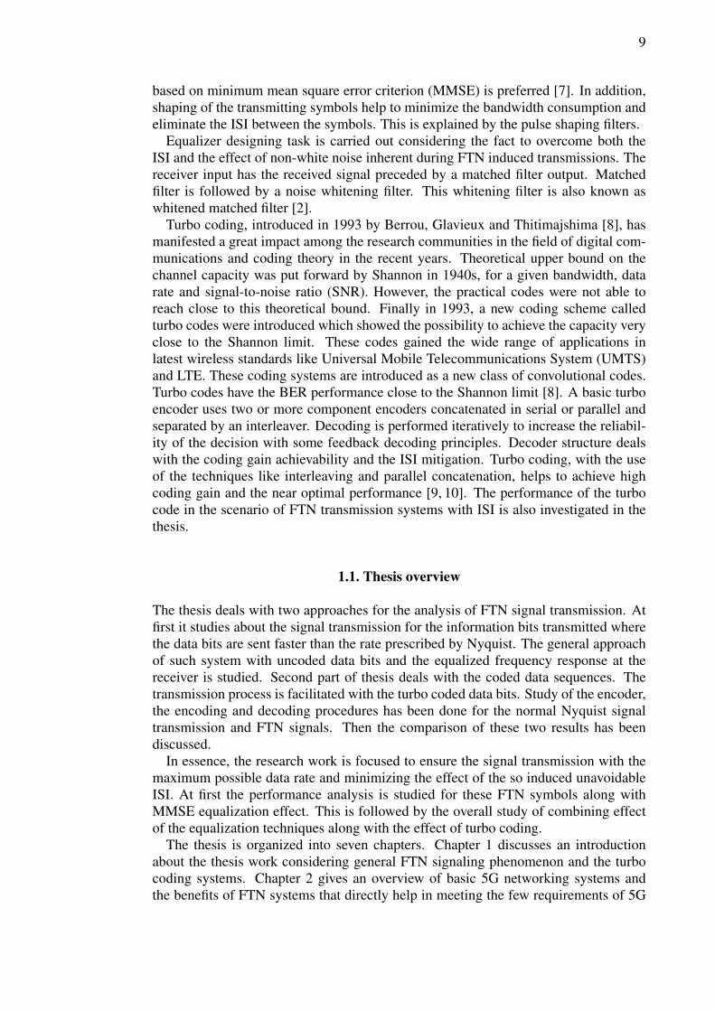
based on minimum mean square error criterion (MMSE) is preferred [7]. In addition,shaping of the transmitting symbols help to minimize the bandwidth consumption andeliminate the ISI between the symbols. This is explained by the pulse shaping filters.

Equalizer designing task is carried out considering the fact to overcome both theISI and the effect of non-white noise inherent during FTN induced transmissions. Thereceiver input has the received signal preceded by a matched filter output. Matchedfilter is followed by a noise whitening filter. This whitening filter is also known aswhitened matched filter [2].

Turbo coding, introduced in 1993 by Berrou, Glavieux and Thitimajshima [8], hasmanifested a great impact among the research communities in the field of digital com-munications and coding theory in the recent years. Theoretical upper bound on thechannel capacity was put forward by Shannon in 1940s, for a given bandwidth, datarate and signal-to-noise ratio (SNR). However, the practical codes were not able toreach close to this theoretical bound. Finally in 1993, a new coding scheme calledturbo codes were introduced which showed the possibility to achieve the capacity veryclose to the Shannon limit. These codes gained the wide range of applications inlatest wireless standards like Universal Mobile Telecommunications System (UMTS)and LTE. These coding systems are introduced as a new class of convolutional codes.Turbo codes have the BER performance close to the Shannon limit [8]. A basic turboencoder uses two or more component encoders concatenated in serial or parallel andseparated by an interleaver. Decoding is performed iteratively to increase the reliabil-ity of the decision with some feedback decoding principles. Decoder structure dealswith the coding gain achievability and the ISI mitigation. Turbo coding, with the useof the techniques like interleaving and parallel concatenation, helps to achieve highcoding gain and the near optimal performance [9, 10]. The performance of the turbocode in the scenario of FTN transmission systems with ISI is also investigated in thethesis.

1.1. Thesis overview

The thesis deals with two approaches for the analysis of FTN signal transmission. Atfirst it studies about the signal transmission for the information bits transmitted wherethe data bits are sent faster than the rate prescribed by Nyquist. The general approachof such system with uncoded data bits and the equalized frequency response at thereceiver is studied. Second part of thesis deals with the coded data sequences. Thetransmission process is facilitated with the turbo coded data bits. Study of the encoder,the encoding and decoding procedures has been done for the normal Nyquist signaltransmission and FTN signals. Then the comparison of these two results has beendiscussed.

In essence, the research work is focused to ensure the signal transmission with themaximum possible data rate and minimizing the effect of the so induced unavoidableISI. At first the performance analysis is studied for these FTN symbols along withMMSE equalization effect. This is followed by the overall study of combining effectof the equalization techniques along with the effect of turbo coding.

The thesis is organized into seven chapters. Chapter 1 discusses an introductionabout the thesis work considering general FTN signaling phenomenon and the turbocoding systems. Chapter 2 gives an overview of basic 5G networking systems andthe benefits of FTN systems that directly help in meeting the few requirements of 5G

10

systems. Chapter 3 is related to the necessary literature review and background studyrelevant to the entire research task. It includes an overview of the signal transmissionand receiving process and also the FTN system. Also turbo codes are discussed in thischapter including the encoder and decoder architecture, the interleaver and decodingphenomenons. System model and the setup environment are explained in Chapter 4.For the performance analysis, the MATLAB implementation details and the simulationresults are given in Chapter 5. This is followed by the discussion of thesis alongwith some future scope of the work in Chapter 6 and finally Chapter 7 concludessummarizing the thesis work.

11

2. 5G NETWORKS AND FASTER THAN NYQUISTSIGNALING

In this chapter, a general description about fifth generation (5G) network is discussed.In addition to this, the basic idea about faster than Nyquist (FTN) is introduced. Fur-thermore, the practicality of FTN signaling is presented to justify its benefit in 5Gnetwork.

2.1. Introduction to 5G Network

Wireless network refers to the communication medium between transmitter and re-ceiver without any physical media but rather through the radio waves and micro waves.5G network does not have specific official standardization mentioned yet. However,it is expected to have the standards much more efficient than the current standard 4GLong term evolution-Advanced (LTE-Advanced) networks. Studies and research onsetting the standard for 5G are basically focused on enhancing the network in termsof bandwidth efficiency, high data rate and also the converged wireless fiber networkfor combining high speed and wide bandwidth feasibility [11]. It is considered as afuture of mobile broadband expected to meet by 2020 [12]. Evolution in the technol-ogy of wireless communications is further targeted to the deployment of 5G networkto connect the entire world more smartly with the advanced telecommunications. It isdesired to improve over mobile and fixed networks with wide range of applications andvarying data rates as required by the user in the multiuser environments. 5G incorpo-rates different wireless technologies to enhance system proficiency and generate moreapplication areas. The international telecommunications union (ITU) is extensivelyworking to introduce the 5G with superfast, all-encompassing features along with thefunctioning of existing trends of 4G and third generation (3G) networks.

Cellular wireless generation has shown its evolution to next stage at around a gap ofa decade starting from first generation (1G) at the beginning of 80’s. From the time of1G where it used analog signals only, with very limited facilities, the wireless networkhas seen a drastic improvement by the time it reached the present digital 4G networkwith extended multimedia services, high data rates and high quality of services (QoS).However, the future world is not satisfying with this achievement. Requirement of thetechnology with better coverage, low latency and extremely high reliability is increas-ing at very fast pace.

Previous mobile telecommunication generations like second generation (2G) werebasically coverage dominated. This concept was changed to be capacity dominatedby the time it reached 3G. At present, the new 4G and upcoming 5G are primarilyconsidered as efficient energy dominated [13]. New innovations of 3rd GenerationPartnership Project (3GPP) standard beyond 4G and LTE-Advanced is to be namedas new generation high bandwidth and high speed internet connectivity technology.Employment of millimeter wave technologies with smart antenna structures, massivemultiple input multiple Output (MIMO) concept, optimizing future PHY/MAC con-siderations, dense network performance improvements and cognitive radio technologyare being studied aggressively to meet the 5G specifications and requirements [14,15].

This new phase of mobile communication comes with the new network architectureconsisting of user terminal and multiple independent and autonomous radio accesstechnologies (RAT) [16]. It is an all internet protocol (IP) based model for wireless

12

and mobile networks interoperability with adaptive new air interfaces and a commonbase for all radio technologies [17]. Additionally, it engulfs the feature of ultra-denseradio networking with self-backhauling, device-to-device communications, dynamicspectrum reframing and radio access infrastructure sharing [16,18]. Wireless networkswith simultaneous connection to multiple wireless technologies and switching amongthemselves is enabled as and when required at high connectivity. Consequently, itprovides the whole wireless world with complete support of multi path technologydeveloping a complete wireless world wide web with an integrated networking.

5G network provides huge broadcasting data speed in the range of Gigabytes. Itis estimated to have 1000 times higher wireless area capacity, 10 Gb/s link speed,lower end to end (E2E) latency by almost 5 times than 4G network and 90% en-ergy saving per provided service [19]. 5G radio access will be modified consideringthe reference with both new RAT and evolved existing wireless technologies (LTE,High Speed Packet Access (HSPA), Global System for Mobile communication (GSM)and WiFi) [14]. The 5G mobile network supports Orthogonal frequency-divisionmultiplexing (OFDM), Ultra-wide band (UWB) Network, Multi-Carrier Code Divi-sion Multiple Access (MCCDMA), IPv6 and Local Multipoint Distribution Service(LMDS) [14,20]. It acts as the ubiquitous mobile ultra-broadband network supportingthe future internet. Current technology is providing the summed up benefit of cloudcomputing, more powerful terminals and high speed connectivity into a single entityas smart devices [15, 18]. Therefore, 5G network is defined to have the unified seamless environment for the integration of different wireless network technologies therebycreating substantial level of improvement in performance and capabilities over existingnetworks.

2.1.1. Challenges

The global race for the introduction of 5G network is expected to come up with thedramatic harmonization and improvement of the radio spectrum which creates newpossibilities for the scenarios like smart cities, remote surgery, driverless cars and thenew approach of internet of things (IoT). This stipulates the fact that the huge rise inthe demand of connected devices is expected to grow up exceptionally. It is estimatedthat the demand for the inter connectivity among devices rise by 50 million to 100million devices by 2020 [21]. In order to meet these expectations, there are manychallenges to be faced, some of which in general are discussed below:

• Requirement is based on the way people use technology to communicate andaccess the information globally. The wireless world created by 5G networkis expected to create an environment requiring very high speed applications.Achieving this high data rate is one of the major challenges.

• Dramatic increase in the traffic volume due to large number of communicat-ing devices require the further expansion of the mobile broadband. However,the bandwidth spectrum is limited. Furthermore, in order to avoid the negativeimpact on mobile services, the spectrum allocation by authorities should be har-monized globally.

• The massive growth in the communication devices regarding capacity, connec-tivity and their diverse use compels to create a new definition to meet the require-

13

ments of future communicating devices. Assurance of efficient QoS, reliabilityand security is required.

• Since 5G network runs under ultra-high spectrum bands, they are more vul-nerable to interferences as they travel longer distances. In addition to this, therequirement to facilitate the high speed data transmission for these densely pop-ulated user devices requires high frequency applications. This creates a greatchallenge to offer the wide range of coverage.

• In addition, 5G network has a challenge of maintaining desired infrastructure tomeet the required specifications. Making common platform or common globalstandard by integrating the diverse standards is an important issue.

2.2. Faster than Nyquist Signaling (FTN) for 5G Network

5G network is a future network with an ambitious goal to achieve high speed giga-byte experience to the users with an increased capacity as compared to current LTEsystems [19]. Support of the wide range of data from low rate application devices tohigh speed communicating multimedia devices is to be addressed. Out of the many ad-vanced technical solutions offered in 5G networks as compared to existing networks,the unimaginably fast speed is one of the prime requirements. The network upgradefor 5G is expected to solve the requirements of most aggravating problems experi-enced today, i.e., the search for a fast and reliable connection. It is considered as thenew wave of digital society, the emerging successor to LTE. The 5G is yet to becomea standard, but the technologies under development for the network has been targetedfor the situation when mobile data traffic will push the LTE networks to their limit.The proposed speed from every individual user in 5G communication system is a greatchallenge. This increased internet data traffic has forced for the intensive research in5G network.

In order to make this high speed transmission achievable, various signal processingtechniques like waveform coding and modulations are performed at the transmitterand receiver structures. One approach is to make the data signals travel at the ratefaster than the conventional methods. Also the spectrum band has a great shortageand thus the regulatory organizations provide limited resources. So within this givenspectrum, signal processing is to be done to increase the transmission speed. Use ofnon-orthogonal pulse symbols for the signal transmission has emerged as one of thenovel solutions to address the issue [1, 6]. These non-orthogonal pulses are referredas FTN pulses where the symbol duration is reduced so as to make more data to betransmitted within the given time frame. This ensures high data rate without reducingthe spectral efficiency.

Thus, in the context of the requirement of high speed communication, study of FTNcomes as a promising approach. This is obtained at the cost of complex receiver struc-tures and processing difficulties.

This thesis work, related to the use of benefits from utilizing faster than Nyquistsignaling, helps to provide high speed data communication and high speed broadbandwireless connection, which is one of the important parameters for the 5G networks.FTN helps the 5G network by assisting the high data rate, high channel capacity andgood error rate performances.

14

2.3. Faster than Nyquist Signaling

2.3.1. Nyquist condition

In general, for the transmission of data over the bandwidth (B = 1/2THz), we ob-serve ISI free received signal, in the condition that it satisfies the Nyquist criteria forthe orthogonal pulse shapes. The received signal in the transmission system can beexpressed as

y(t) =∞∑

n=−∞

x[n] · h(t− nTs) + ω(t), (2.1)

where x[n], y(t), h(t) and ω(t) denote the transmitted symbols, received signal, im-pulse response (or pulse shape) and noise respectively.

Now, sampling equation (2.1) leads to

y(kTs) =∞∑

n=−∞

x[n] · h(k − n)Ts

= x[k] · h(0)︸ ︷︷ ︸Desired

+∑n 6=k

x[n] · h(k − n)Ts︸ ︷︷ ︸UnwantedISI

.(2.2)

The first term in the equation (2.2) represents the desired signal component whilethe second term represents the unwanted inter-symbol interference (ISI). In order toget rid of this ISI, the pulse response h[n] must satisfy

h[n] =

{1 n = 00 n 6= 0.

(2.3)

Also its corresponding frequency domain representation can be written as,

h(t) ·∞∑

k=−∞

δ(t− kTs) = δ(t) (2.4)

which is equivalent to equation (2.3).Now the Fourier transformation is expressed as

H(f) ∗ 1/Ts

∞∑k=−∞

δ(f − k/Ts) = 1. (2.5)

Using the shifting property, the equation can be derived as,

1

Ts

∞∑k=−∞

H(f − k/Ts) = 1. (2.6)

15

This is the condition to be satisfied by the channel frequency response to ensure an ISIfree transmission. Since the pulse h(t) is orthogonal (Nyquist condition satisfied), theoptimum detection of such signals can be performed in a symbol by symbol way usingthe sampler and the filter matched to h(t) [6].

2.3.2. FTN Scenario

The concept of FTN as quoted by J. E. Mazo in 1975 [3] gives a motivation to studyits optimal performance criteria when the signal transmission is carried out at the ratefaster than the conventional rate which is satisfied by the Nyquist condition. Accordingto Mazo, increasing the rate of transmission of the signal by 25% more than given byNyquist rate does not degrade the minimum Euclidean distance. In other words, Mazoclarifies that for Sinc pulses, in binary signal transmission, even with the increase inthe signaling speed or increasing the rate of data transmission beyond the Nyquistsignaling condition, minimum Euclidean distance does not reduce much.

FTN refers to the system in which the signal is transmitted with the symbol in-terval T0 < T , where T refers to the symbol interval for the condition which satisfiesNyquist criteria and T0 is the new symbol interval for FTN. Reducing the symbol inter-val converts the Nyquist orthogonal pulses to non-orthogonal. This mechanism offersan advantage that more symbols can be transmitted in a given time frame as comparedwith the conventional arrangement. Thus more information can be transmitted at therate faster than prescribed by Nyquist criteria. The equation for system with ordinaryNyquist condition

y(t) =√Es∑n

x[n] · h(t− nT ) (2.7)

can be modified for FTN as

y(t) =√Es∑n

x[n] · h(t− nαT ). (2.8)

In the equation (2.8),√Es represents the symbol energy, α is the factor which deter-

mines symbol time αT (equivalent to T0), where α < 1.Lower the value of α, the more will be the data rate but at the same time error rate

is increased. Thus it comes as a tradeoff between these two parameters.Unlike the ordinary linear modulation, FTN signaling system contains the pulses

which are non orthogonal with respect to symbol time. The non orthogonal pulsesused by FTN cause the sent symbols to be overlapped partially or fully dependingupon the symbol interval T0. This gives rise to an unavoidable ISI, which causes adegradation of the system performance. To get the benefits of FTN, these ISI needsto be eliminated. This is achieved at the cost of higher receiver complexity. Differentreceiver processing techniques are implemented to simplify the process.

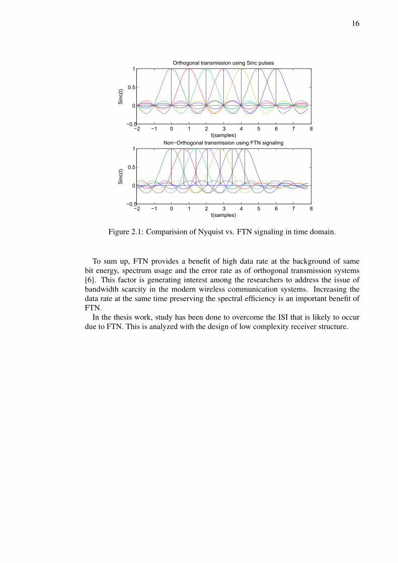
Figure 2.1 shows the representation of the orthogonal and the nonorthogonal sig-nals in their corresponding time domain. As seen in the Figure 2.1, with an orthog-onal transmission using Sinc pulses, since the pulses are orthogonal, ensures no ISIscenario. However, in the context of non orthogonal transmission using FTN signal-ing, it is clear that due to the non-orthogonal pulses, time required to transmit sameamount of pulse symbols is reduced as compared to previous one. But due to thenon-orthogonality of the pulses, ISI is introduced.

16

−2 −1 0 1 2 3 4 5 6 7 8−0.5

0

0.5

1Orthogonal transmission using Sinc pulses

t(samples)

Sin

c(t)

−2 −1 0 1 2 3 4 5 6 7 8−0.5

0

0.5

1Non−Orthogonal transmission using FTN signaling

t(samples)

Sin

c(t)

Figure 2.1: Comparision of Nyquist vs. FTN signaling in time domain.

To sum up, FTN provides a benefit of high data rate at the background of samebit energy, spectrum usage and the error rate as of orthogonal transmission systems[6]. This factor is generating interest among the researchers to address the issue ofbandwidth scarcity in the modern wireless communication systems. Increasing thedata rate at the same time preserving the spectral efficiency is an important benefit ofFTN.

In the thesis work, study has been done to overcome the ISI that is likely to occurdue to FTN. This is analyzed with the design of low complexity receiver structure.

17

3. LITERATURE STUDY

This chapter covers the related literature review required for the analysis of the the-sis work. In general, the different terminologies and processing theories required forthe understanding of signal transmission under the constraint of Nyquist criteria andFTN transmission system are presented. Theories behind the implementation of turbocoding system to analyze the coded transmission system under FTN scenario is alsodiscussed.

3.1. Nyquist Signaling

In the study of signal processing, we define the Nyquist rate as the rate which is twicethe bandwidth of a band limited signal or a channel. It can be conceptually studiedrelating the Nyquist rate in accordance with signaling and sampling as two differentapproaches.

From the sampling point of view, it is defined that in order to have no aliasingeffect, the minimum sampling rate should be equal to or greater than double the highestfrequency component contained within the signal. This means that sampling rate mustbe higher than the Nyquist rate. Sampling process involves the discretization of thecontinuous time signals. These samples are to be taken in a manner that it representsthe original signal significantly. The number of samples taken defines the signal ratefor specific signal bandwidth.

Nyquist signaling or Nyquist pulse shaping criteria highlights the necessary andsufficient condition so as to achieve zero ISI scenario. In the Nyquist paper [22], itis described about the number of pulses that could be transmitted and received over aband limited channel and also the rate of transmission. In the paper, the Nyquist signal-ing rate is defined as the maximum possible pulses that could be transmitted througha given bandwidth limited channel. This gives an idea about the Nyquist signaling,which provides platform for the design of the modern communication systems.

Nyquist rate clarifies the concept defining the rate as lower bound for the samplerate and upper bound for the symbol rate in a bandwidth constrained baseband channelwithout ISI. The upper limit for the number of bits per signal change is defined bythe channel characteristics which is also known as the Shannon limit [23]. In short,the sampling frequency greater than twice the bandwidth is the condition where noaliasing effect occurs indicating the fulfillment of the Nyquist criteria. This means thatfor the continuous function x(t) sampled at fixed sampling rate, the function that isband limited to 1/2fs only satisfies the Nyquist condition, i.e., its Fourier transform

X(f) = 0 for all |f | ≥ 1/2fs. (3.1)

For B ≤ 1/2fs, 2B and 1/2fs are the expressions defining Nyquist rate and frequencyrespectively, where the symbol T = 1/fs represents the sample period or the samplinginterval and B is the bandwidth.

3.1.1. Necessary and sufficient conditions for Nyquist criteria

In a wireless communication, when the linearly modulated symbols are transmitted,the channel impulse response or the frequency response spreads the transmitted signal

18

in time domain. Such consecutive symbol transmission can create aliasing effect aspreviously transmitted signal may overlap over the other later signal. Nyquist crite-rion indicates the condition which when fulfilled, provides the zero ISI during suchtransmission.

As seen from the derivation in section 2.3, we can define the Nyquist ISI criteriaas, for the discrete signals, x[n] = x(nTs) and the channel impulse response h(t) =h(nTs), the necessary and sufficient Nyquist condition for zero ISI or pulse shapingcriteria stipulate that for a given pulse h[n], it has to satisfy [2]

h[n] =

{1 n = 00 n 6= 0

(3.2)

and its Fourier transform satisfy

1

Ts

∞∑k=−∞

H(f + k/Ts) = 1 (3.3)

which means that the frequency shifted versions ofH(f), the fourier transform of h(t),is summed up to 1.

The relation (3.3) gives information that the Nyquist criterion is the condition ofa wireless channel threshold for designing transceiver structures to attain an ISI freetransmission. Nyquist first criterion [24] explains that the contributions at the samplinginstant (T, 2T, 3T...) of the received waveform must be zero. Equations (3.2) and (3.3)indicate the fact that the sum of delayed pulse spectra by k/T should sum up to T or aconstant. Raised cosine pulses are such commonly used practical pulses that meet theNyquist ISI criterion. This is discussed later in section 3.4.

3.2. Pulse shaping filters

Considering a situation for increasing data rate or transmission rate for a system withgiven (fixed) bandwidth without accuracy degradation, we see the bandwidth con-straint to be constant. One possible way is to modify the pulses effectively such that itrequires less bandwidth than the contemporary means. The pulse shape is desired to besmooth. The distorted shape may deteriorate the condition requiring larger bandwidthsince such shapes contains the energy spectrum including lower frequency harmoniccomponents. It is required that, at the perfect scenario, transmitted pulse do not inter-fere each other at the receiver with the successive symbols being received. The erroroccurred during this procedure is termed as ISI. So it is somewhat like a tradeoff be-tween the gain and complexity. In order to have smooth shape for spectral efficiency,pulse shaping filter is selected such that it can transform the given waveform into thedesired form.

The transmitted signals are the result of the data pulse passed through a pulse shap-ing filter which is responsible for defining the transmitter spectrum. They have a role ofallocating the prescribed signal in a defined bandwidth minimizing the spectral leakageand also to maintain the high transmission rate and low error rate for a signal. In a sys-tem with band limited channels, during the increased modulation rate of a transmittedsignal, it is highly probable to have distortion or the ISI due to bandwidth limitation.So it requires fixing the transmitted waveform into the shape such that signal remains

19

in the prescribed bandwidth. Ideal filters undergo a proper sampling procedures toensure the minimum ISI and high stop band attenuation to reduce the inter channelinterference (ICI) [25].

Usually a rectangular ideal pulse is desired over an interval [0, T ] but the pulses hav-ing different functional forms for, e.g., Sinc pulses have the spectrum with side lobesdecreasing with frequency. This causes an unintentional overlapping of the symbolsfrom the adjacent channels or the signals. Ideally we expect the pulse with peak att = 0 and zero at other sampling instants t = T, 2T, 3T.... In time domain it hasto satisfy that its impulse response has periodic zero and zeros must occur at othersampling times, i.e., h[nT ] = 0, where T is the data sample period. Pulses bearingsuch characteristics are referred as Nyquist pulses and the corresponding filters bear-ing such impulse responses are called Nyquist filters [26]. The pulse shaping filters aredesigned to satisfy the Nyquist ISI criterion.

When the band pass filtering is done prior to matched filtering, these filters reducethe cost of hardware designs as well. Pulse shaping filters implemented in frequencydomain make it easy to recover the information embedded in the carrier signal byexploiting the frequency diversity at the receiver end using the signal decompositionor recombination [27].

For optimal filter design, the delta function δ(t) with pulse information is sent fromthe transmitter end. The full signal recovery ideal output then should be δ(1 + σ),where σ is the time delay of the causal system. Consequently, at the receiver end,there should be ideal output δ(t) [28].

Usually these pulse shaping filters at the transmitter is used in reference to the corre-sponding matched filter at the receiver unit for optimal performance. Many pulse shap-ing filters like Sinc shaped filter, rectangular pulse filter, Raised-cosine filter, Gaussianfilter are in practice.

Here, in the thesis work, raised cosine filters are used for its best suitability satisfyingNyquist criteria and the spectral efficiency.

3.3. Roll-off factor

Roll-off factor gives the measure of the excess bandwidth occupied by any digital filteras compared to that of theoretical minimum Nyquist bandwidth. Bandwidth utilizationis very important in wireless communication. In real time communication, the signalsusually tend to occupy the bandwidth more than specified by Nyquist bandwidth. Thisexcess value is referred as the roll-off factor. For, e.g., any digital filter with 100MHz Nyquist bandwidth if occupies 130 MHz, is said to have roll-off factor 0.3 whichmeans the filter excess bandwidth is 0.3 times the Nyquist bandwidth. It can also bedefined as the steepness measure in the transition between the stop band and pass bandof the filters. It directly relates to the bandwidth saving strategy. Bandwidth savingbetween two spectral roll-off factors can be calculated as [29]

Bandwidth saving (%) = 100− ((β1/β2)× 100). (3.4)

Here, β1 is referred from the lower value between the two roll-off factors. Mathe-matically roll-off factor can be related as, for the Nyquist bandwidth of 1/2T , if theexcess bandwidth as compared to this Nyquist bandwidth be ∆f , then the roll-off fac-

20

tor (β) is given by

β =∆f

1/2T=

∆f

Rs/2= 2T∆f, (3.5)

where 1/T is the symbol rate. The value of β lies between 0 and 1. It is an importantmodulation parameter to determine the signal bandwidth and spectral efficiency.

Variation in the values of roll-off factor causes a change in the characteristics ofmodulated signal which directly affects the impact of the transmission signal. Higherroll-off means low ISI, since it reduces the change rate of the amplitude of output pulseat zero crossings. But it makes the signal bandwidth wider consequently consuminglarger spectrum. On the other hand, lower the value of roll-off factors designed, higheris the spectral efficiency achieved. However, the rate of signal decay is slowest in thetime domain. This makes the baseband signal more complex. In short, comparativelower roll-off values means a corresponding decrease in bandwidth usage and increasein symbol rate and overall throughput. This highlights that the proper selection ofroll-off factor plays an important role on the performance of the system designed.

The maximum symbol rate Rs attainable as studied in [30] can be related from roll-off factor for the given bandwidth as

Rs = B(1 + β), (3.6)

where B is the bandwidth of the system and β be the roll-off factor.

3.4. Raised cosine pulse

Raised cosine (RC) filters are known for their ability to reduce the inter symbol inter-ference of the signal. In communication systems, they are used as pulse shaping filtersto shape the pulses. Basically the name raised cosine stands for non-zero portion of thefrequency spectrum with roll-off factor equal to 1 which defines the cosine functionraised above the horizontal axis. It is the representation of pulse spectrum. For thechannel with bandwidth B, if T > 1/2B then the pulse spectrum for this condition iscalled the raised cosine spectrum where 1/T is the sampling rate of the signal.

Raised cosine pulse shaping modulation is bandwidth efficient, i.e., more bits/sec/Hzand also power efficient, i.e., it requires comparatively low Eb/N0 for same bit er-ror rate. These pulses stand as a balance between the rectangular pulse and the Sincpulses. Rectangular pulses have sharp edges in the time domain indicating the largebandwidth in the frequency domain. So it requires infinite bandwidth. On the otherhand, Sinc pulses have an infinite length of time domain sequence. Raised cosinepulses are therefore preferred as they exhibit the balanced nature between these twopulses. These pulses do not show such infinite long nature in both the time and fre-quency domains. When the passband frequency of these filters is half the data rate, itsatisfies the Nyquist criterion such that T = NTs [31], where T is the data period andN is any integer.

21

Frequency response characteristic of a raised cosine function is given by [2]

Xrc(f) =

T for 0 ≤ |f | ≤ 1−β

2T

T2{1 + cos(πT/β(|f | − 1−β

2T))} for 1−β

2T≤ |f | ≤ 1+β

2T

0 for |f | > 1+β2T ·

(3.7)

In the relation (3.7), β is the roll-off factor and T is the reciprocal of symbol rate.Impulse response of the spectrum for raised cosine function is given by [2]

x(t) =sin(πt/T )

πt/T

cos(πβt/T )

1− 4β2t2/T 2

= Sinc(πt/T )cos(πβt/T )

1− 4β2t2/T 2·

(3.8)

As seen in the equation (3.8), the raised cosine pulse takes the form of a Sinc pulseshapes. The bandwidth of the pulse and the rate of decay are determined by the valueof roll-off factor (β). Lower the value of β, sharper the spectrum . With roll-off value1, it gives the pure raised cosine spectrum removing the flat portion. The tails of thesignal x(t) is decayed as 1/t3 for roll-off factor greater than zero. This is the reasonbehind the formation of ISI which is formed when the timing mismatch occurs duringsampling. Since the impulse response of RC filters has indefinite structure, it needs tobe truncated for practical applications. In frequency domain, this truncation yields anon zero side lobe. However, since pulse response delay is proportional to 1/t3 , theresult might vary from that of theoretical approach [26].

Ideal response of a raised cosine filter has a unity gain in the region of low frequencyand total attenuation at the high frequency. In the middle of these two frequencies,responses has a raised cosine function, size of which is determined by the roll-offfactor. So they are also called low pass filters. This raised cosine function meets therequirement of a pulse shaping filter, i.e., low pass response in frequency domain, zeroISI case and finite extent in time domain [26].

For an ideal channel,

Xrc(f) = Gt(f)Gr(f), (3.9)

where Gt(f) and Gr(f) are the frequency responses of the transmitter filter andreceiver filter respectively [2]. These filters are used to analyze the overall desiredfrequency response.

For the matched condition of transmitter and receiver filter, Gt(f) = G∗r(f) whichyields,

Gt(f) =√|Xrc(f)|e−j2πft0 .

(3.10)

Here, t0 is the nominal delay that is introduced to ensure the physical realizability ofthe filter [2].

The ISI free nature of raised cosine filter is the main reason behind its wide usein communication systems [32]. Using these filters, matched filtering is performed

22

−10 −8 −6 −4 −2 0 2 4 6 8 10−0.4

−0.2

0

0.2

0.4

0.6

0.8

1

time, t

ampl

itude

, g(t

)

Time domain waveform of raised cosine pulse shaping filters

beta=0beta=0.5beta=1

Figure 3.1: Time domain representation of Raised Cosine Pulse.

0 0.2 0.4 0.6 0.8 1 1.2 1.4 1.60

1

2

3

4

5

6

7

8

9

frequency, f

ampl

itude

, |G

(f)|

Frequency domain representation of raised cosine pulse shaping filters

beta=0beta=0.5beta=1

Figure 3.2: Frequency domain representation of Raised Cosine Pulse.

in the receiver to reduce the error in the received signal. Matched filter in this case

23

reduces the noise by creating a low pass filter and also helps in ISI reduction, which isdiscussed more in section 3.5.

Currently the new families of raised cosine filters are under research which not onlyprovide zero ISI but also help to decrease the peak-to-average ratio (PAR) of the base-band signal over the conventional ones [33]. The time and frequency domain repre-sentations of raised cosine pulses are shown in Figures 3.1 and 3.2, respectively.

3.4.1. Root raised cosine pulse

Like the raised cosine, root raised cosine (RRC) also called as square root raised cosineare the pulse shaping filters that help to reduce the ISI. Basically, they are the squareroot of the frequency response of raised cosine functions. For an ISI free transmission,the response of transmit filter, receive filter and the channel has to satisfy the NyquistISI criteria. Designing the matched, transmitter and the receiver filter such that theircombination satisfy the Nyquist condition is an important task in defining wirelesscommunication systems. The RRC pulse do not have the perfect orthogonal pulses,i.e., the impulse response is not equal to zero at every symbol time interval T, 2T, ...and so on. However, the combined effect of these RRC pulses at the transmitter andreceiver shows the characteristics of Nyquist filter thereby helping to minimize the ISI.

In a practical approach, the root raised cosine filter is used at the transmitter as apulse shaping filter and also at the receiver as a matched filter. When a signal passesthrough these two identical filters, the effects of those filters are squared. This ul-timately provides the total effect of raised cosine filter with an additional benefit ofnoise filtering at the receiver [34].

Frequency response and impulse response of an RRC pulse are given by the equa-tions (3.11) and (3.12), respectively [31]

F (ω) =

1 , ω < ωc(1− β)0 , ω > ωc(1 + β)√

1+cos(π(ω−ωc(1−β))

2βωc)

2, ωc(1− β) < ω < ωc(1 + β),

(3.11)

h(t) =4β

π√T

cos (1+β)πtT

+ T4βt

sin (1−β)πtT

1− (4βt/T )2. (3.12)

The RRC filters provide a practical means for eliminating the side lobes of a spec-trum. This is beneficial for the signal transmission as it has to work on a limitedbandwidth. For the practical implementations, i.e., to make the filter causal, some de-lay is added to the pulse. Since the RRC pulses are non-causal, they are truncated soas to make them physically realizable.

Filtering is required both at the transmitter as well as at the receiver end. The noiseand the interferences at the receiving side are filtered out by the receiver filter. Thefilter effect is viewed as the combined effects of these two transmit and receive filters.Both of these filters should abide by Nyquist criteria. The combined result due to thesetwo filters is expressed as in the equation (3.9) as

Xrc(f) = Gt(f)Gr(f),

24

whereGt(f) andGr(f) are the transfer function of the transmitter filter and receiverfilter, respectively, in frequency domain. Ignoring the effect of frequency domain trans-fer function due to channel and assuming that the transmit filter is equivalent to receivefilter, since Gt(f) = Gr(f) the combined effect is therefore given by

Xrc(f) = Gt(f)Gr(f) = |Gt(f)|2. (3.13)

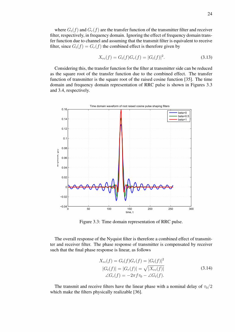
Considering this, the transfer function for the filter at transmitter side can be reducedas the square root of the transfer function due to the combined effect. The transferfunction of transmitter is the square root of the raised cosine function [35]. The timedomain and frequency domain representation of RRC pulse is shown in Figures 3.3and 3.4, respectively.

0 50 100 150 200 250 300−0.04

−0.02

0

0.02

0.04

0.06

0.08

0.1

0.12

0.14

0.16

time, t

ampl

itude

, g(t

)

Time domain waveform of root raised cosine pulse shaping filters

beta=0beta=0.5beta=1

Figure 3.3: Time domain representation of RRC pulse.

The overall response of the Nyquist filter is therefore a combined effect of transmit-ter and receiver filter. The phase response of transmitter is compensated by receiversuch that the final phase response is linear, as follows

Xrc(f) = Gt(f)Gr(f) = |Gt(f)|2

|Gt(f)| = |Gr(f)| =√|Xrc(f)|

∠Gr(f) = −2πfτ0 − ∠Gt(f).

(3.14)

The transmit and receive filters have the linear phase with a nominal delay of τ0/2which make the filters physically realizable [36].

25

0 0.2 0.4 0.6 0.8 1 1.2 1.4 1.60

0.5

1

1.5

2

2.5

3

3.5

4

frequency, f

ampl

itude

, |G

(f)|

Frequency domain representation of root raised cosine pulse shaping filters

beta=0beta=0.5beta=1

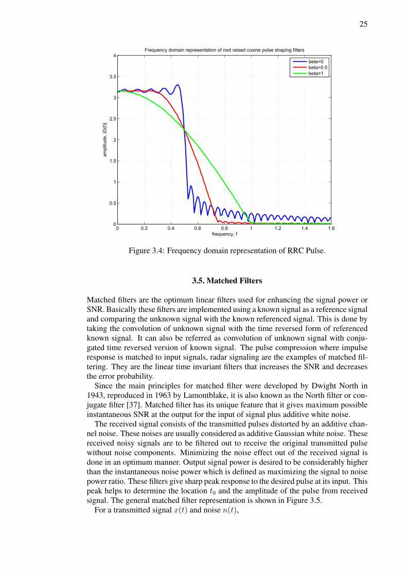
Figure 3.4: Frequency domain representation of RRC Pulse.

3.5. Matched Filters

Matched filters are the optimum linear filters used for enhancing the signal power orSNR. Basically these filters are implemented using a known signal as a reference signaland comparing the unknown signal with the known referenced signal. This is done bytaking the convolution of unknown signal with the time reversed form of referencedknown signal. It can also be referred as convolution of unknown signal with conju-gated time reversed version of known signal. The pulse compression where impulseresponse is matched to input signals, radar signaling are the examples of matched fil-tering. They are the linear time invariant filters that increases the SNR and decreasesthe error probability.

Since the main principles for matched filter were developed by Dwight North in1943, reproduced in 1963 by Lamontblake, it is also known as the North filter or con-jugate filter [37]. Matched filter has its unique feature that it gives maximum possibleinstantaneous SNR at the output for the input of signal plus additive white noise.

The received signal consists of the transmitted pulses distorted by an additive chan-nel noise. These noises are usually considered as additive Gaussian white noise. Thesereceived noisy signals are to be filtered out to receive the original transmitted pulsewithout noise components. Minimizing the noise effect out of the received signal isdone in an optimum manner. Output signal power is desired to be considerably higherthan the instantaneous noise power which is defined as maximizing the signal to noisepower ratio. These filters give sharp peak response to the desired pulse at its input. Thispeak helps to determine the location t0 and the amplitude of the pulse from receivedsignal. The general matched filter representation is shown in Figure 3.5.

For a transmitted signal x(t) and noise n(t),

26

Signal x(t)

Noise

n(t)

Received

signal s(t) Matched

Filter

H(w)

Output y(t)

Figure 3.5: Basic representation of a matched filter.

s(t) = x(t) + n(t)

filter output, y(t) = s(t) ∗ h(t).(3.15)

Since the filter is linear, output can be written as,

y(t) = x(t) ∗ h(t) + n(t) ∗ h(t)

= x0(t) + n0(t).(3.16)

Now the matched filter is the linear filter h(t) or equivalently H(ω) that maximizesthe SNR.

Let the input signal for matched filter be represented by

x(t) = Csi(t− t1) + ni(t), (3.17)

where t1 is the unknown time delay, ni(t) is the input white noise andC is any constantvalue.

Now for the white input noise, its autocorrelation and power spectral density (PSD)functions can be written as

Rni(t) =N0

2δ(t)

Sni(ω) = N0/2,(3.18)

where N0 is a constant value. Output can then be written as, [38]

y(t) = Cso(t− t1) + no(t)

so(t) = si(t) ∗ h(t)

no(t) = ni(t) ∗ h(t).

(3.19)

Here h(t) is the impulse response and * denotes convolution operation.SNR of the matched filter depends on the ratio of signal energy to the PSD of the

white noise at filter output. The signal component with maximum energy occurs at thesampling instant t = T . In matched filter, output is proportional to the shifted versionof the auto correlation function of input signal [39].

27

Matched filters are used considering the noise as white noise. However, if the noiseis colored, the problem is solved by using the filter, known as whitening filter, whichfilters the input signal noise to make it white.

Matched filters are the optimal equalizers used to maximize the SNR at each beamformer output beam when the impulse response is known and the noise is additivewhite noise. Since each different signal requires different filters, it is called matchedfiltering as it has to match all the waveforms. These filters, however, do not play role inminimizing ISI. Since the optimization procedure in matched filter assumes only onesignal transmitted over a channel, it does not focus much with ISI [40]. It enhances theSNR by improving the received signal and not the noise.

3.6. Whitening filters

In any communication systems, noise is always an unavoidable parameter, which ispresent in the received signal that deteriorates the quality of signal power. Since itdegrades the throughput of the system, it needs to be minimized. White noises arethe ones with flat power spectrum having constant power at all the frequencies, i.e.,they are random signal with constant power spectral density. They can also be con-sidered as a sequence of serially uncorrelated random variables having zero mean andconstant variance. Unlike this, colored noise is the one with varying power spectrum.Such noises increase inefficiency of the system. So it is imperative to whiten the col-ored noise. The filters that implement this process of whitening the noises are calledwhitening filters.

Whitening transformation is basically inferred as the decorrelation transformationof random variables with known covariance matrix into new set of random variableswith identity matrix as its new covariance. This transforms the noise vector into awhite noise vector, hence the name whitening filter. They are uncorrelated and havethe variance equal to unity. Whitening filters can help minimize the interference due toother users in spread spectrum communication systems. The process is also known asdigital whitening. During whitening, first the interfering signals are estimated and thenthe coefficients to be used in transversal filter are computed which is then followed bythe filtering procedures for the received signal. In Figure 3.6, r(t) is the received signal

r(t)=s(t)+w(t)sg(t)=s(t)*g(t)

sg(t)+n(t)

Whitening Filter

g(t)

Figure 3.6: Basic flow for Whitening Filter.

comprising of signal s(t) with colored noise w(t), is passed through a whitening filterto get the whitened output signal. The term g(t) indicates the whitening filter and n(t)is the white noise having unit spectral density.

These filters can also be considered as an inverse of the system that distorts it. If thefrequency response of the system isH(Z), then the white filter response is 1/H(Z). In

28

whitened matched filter model, noise whitening filter is introduced after the sampledmatched filter. To be useful in practice, the whitening filter should be stable and causalas well.

If the filter g(t) is used to whiten the noise in order to produce the output noisehaving power spectral density S0

n(f) = N0/2 , then the filter should have [41]

Sn(f)|G(f)|2 = N0/2

i.e. |G(f)|2 = N0/2 · 1/Sn(f),(3.20)

where g(t) is the impulse response of filter, G(f) is its transfer function which changethe power spectral density Sn(f) of the Gaussian noise process with noise N(t).

3.7. Equalizers

Wireless communications is very likely to face different frequency dependant phaseand amplitude distortions due to multipath signal transmissions and fading. In signaltransmission, the received pulses come in a distorted form than the original transmittedpulse. The transmission characteristics of a band limited channel or channel noisegives rise to an ISI which is the cause for the distortion of the signals. Design of theinverse filter to counterfeit the channel impulse response so as to compensate the errorand retain the signals as a replica of original signal is the main task of an equalizer.

Usually the signals are given a pattern through a pulse shaping filter. Proper sam-pling of the signals with no addition of the noise yields no ISI scenario. However, ifit is not sampled at the sampling interval or against the Nyquist condition, the signalreconstruction is not exact. Moreover, the addition of channel noise causes a distortionin signal regenerating process at the receiver. To overcome this situation, the distortedsignal is passed through a filter which is basically a multiplicative inverse in spectraldomain of the frequency response of a channel. This is called equalization. Thus theequalized output is considered as reliable output.

Generally for short range transmissions, preset equalizers are used since in such casechannel characteristics is not an important factor that needs to be considered. This isbecause the channel parameters are more or less time invariant. For the long rangecommunications, the equalizers must be adaptive such that equalizers adapt to the timevarying characteristics of the channel. The equalizer adjustment algorithms are mainlybased on either peak distortion criteria or mean square distortion criteria [42].

In a communication system, considered linear time invariant, output signal can bemodeled as

x[n] =∞∑

k=−∞

h[k]s(n− k) + v(n), (3.21)

where s[n] is the transmitted symbol, h[k] the impulse response and v[n] is additivewhite gaussian noise (AWGN). Now equation can be simplified as,

x[n] = h[0] + s[n] +∞∑

k=−∞,k 6=0

h[k]s(n− k) + v(n). (3.22)

29

In equation (3.22), the second part of the equation refers to the delayed version ofthe transmitted symbols, which are known as inter symbol interferences. The equalizeris focused to eliminate this ISI to the minimum level possible.

Various equalization methods are implemented as demanded by the situation of sig-nal transmitting and receiving procedures. In the thesis work, MMSE equalizationmethod is effectuated.

3.7.1. MMSE equalization

In digital communications, equalizers come along with matched filters where equaliz-ers are responsible to minimize ISI and the matched filters reduce the channel noise.Equalizers can be classified based on their structure, algorithms used to adapt the co-efficients or their optimization criteria. MMSE algorithm makes use of the joint mini-mization of noise and ISI parameters.

MMSE equalization is considered as a measure of estimator quality. It is based onMMSE filtering. The linear filter which is designed to minimize the error between thetransmitted signal and the received output such that original signal can be estimatedout of it are the MMSE filters. The error consists of an ISI in addition to the noise.The MMSE criterion ensures an optimum tradeoff between the residual ISI in the re-ceived signal and noise enhancement. In such equalization, since the minimization ofmean square error (MSE) is done, the noise amplification is reduced. This is why itoutperforms the zero forcing equalizers.

The main objective of the MMSE equalizer is to minimize the variance of the errorsignal or the the mean square value of the error. The error signal is calculated by thehelp of estimated signals. It is the difference of transmitted signal and the estimate ofthe received signal. At low to moderate SNR values, these equalizers give remarkablylower bit errors as compared to zero forcing equalizers

el = sl −Gl,lRl

Jl = E|e|2.(3.23)

In the relation (3.23), Jl is mean square error, Gl,l is equalizer coefficient, sl is thetransmitted signal, Rl the estimate of received signal and el is the error. Minimizingthe mean square error can be done using the orthogonality principle which states thatmean square error Jl is minimum if the equalizer coefficient Gl,l is selected in a waythat received signal Rl and error el are orthogonal to each other [43]

E[elR∗l ] = 0. (3.24)

Now the equalizer coefficient for the MMSE equalization is calculated by the equa-tion

Gl,l =H∗l,l

|Hl,l|2 + σ2, (3.25)

where H represents the channel matrix with the diagonal components Hl,l and σ2 rep-resents the noise variance.

30

Equation (3.25) infers that MMSE computation needs the value of noise variance(σ2), which is determined during the system design that helps MMSE equalizer givethe optimal performance.

3.8. Turbo coding

Coding basically refers to the mechanism where information sequences are encodedin a manner such that when transmitted over noisy channel, still retains the originalsignal at the decoder when decoded. Usually coding is viewed as the source codingand channel coding. Source coding refers to the modification of message source to thecode in the form that could be transmitted through channel. Channel coding meansthe encoding of the message that results from source coding such that by introducingsome form of redundancy, error correction and message detection is done reliably atthe receiver.

Turbo codes from the time of its introduction [44, 45] are gaining interest in theresearch field and investigation of coding theory as a new approach to error correctioncode. This is due to its high coding gain and near Shannon capacity performance.

Turbo codes are the derivation of convolution codes, class of high performance for-ward error correction (FEC) codes. These convolution error correcting codes use a softiterative decoding procedures resulting in the high coding gains than the conventionalconvolution codes. They offer a wide range of wireless communication applicationsapplicable from 3G mobile systems to deep space explorations. Turbo codes are usedextensively in modern wireless communication systems like LTE and LTE-A. Basi-cally, it consists of recursive systematic convolution (RSC) encoder, interleaver andan iterative decoder. Using an iterative a posteriori probability (APP) decoder wasintroduced which provided low BER at the SNR very close to Shannon theoreticallimit [45]. Maximum a posteriori (MAP) algorithm was used for the coded sequencesby Bahl Cocke Jelinek Raviv (BCJR) [46]. These error correction codes are widelyused in the field areas which expect a good power saving scenario and low SNR re-quirement. Parallel concatenated turbo codes, serial concatenated turbo codes, andrepeat-accumulate codes are some of the examples of turbo code implementation.

During coding, the information bits are mapped to the code bits. This is done byconvolving the information bits with the generator sequence code bits. Turbo codesare preferred over the other FEC codes as they provide better result compared to othersat least by 3 dB, saving approximately 20% of bandwidth spectrum [47].

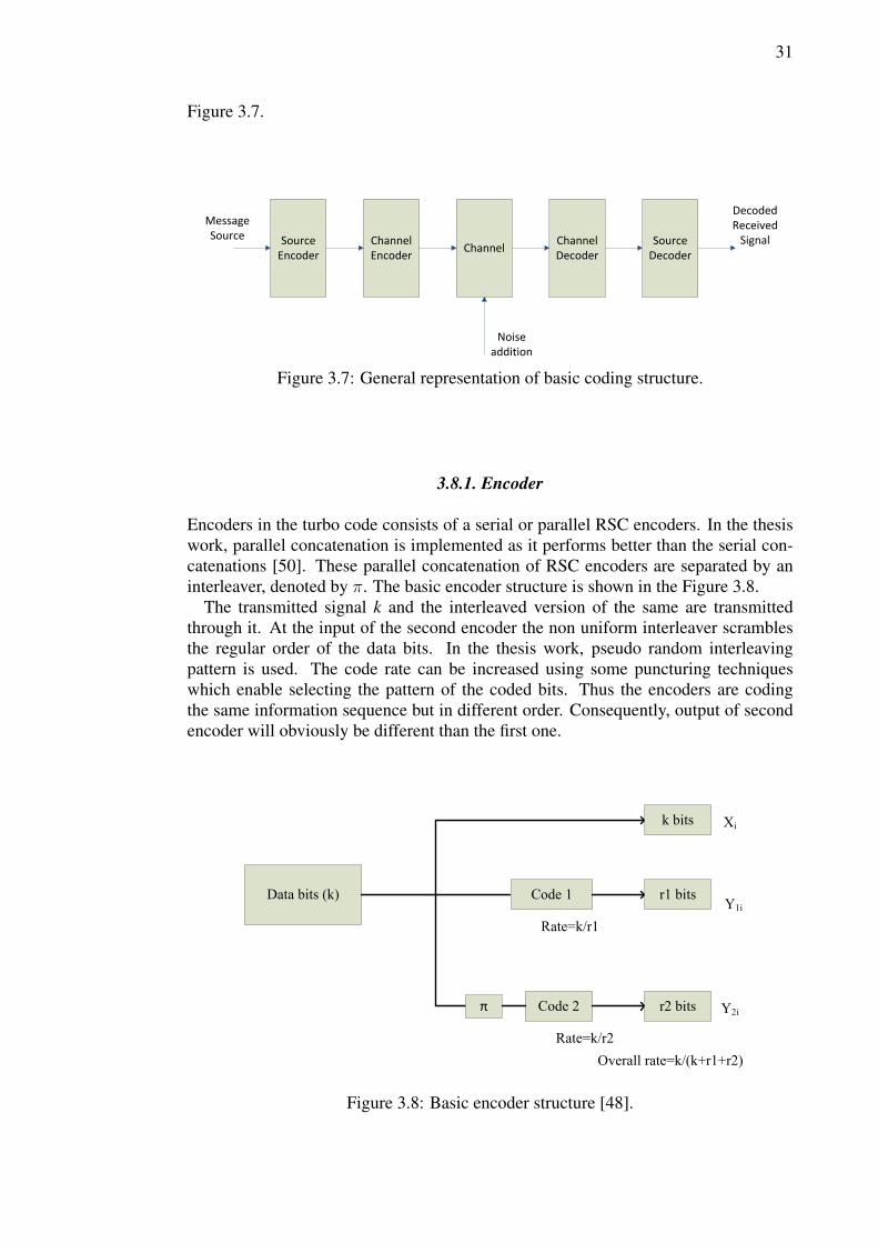
Code rate is used to explain the redundancy of the code. Turbo codes used in thethesis are the parallel concatenated convolution codes with rate k/n, where k andn denotes the information bit sequence in the encoder and output bits, respectively.Check sequences transmitted together, also called as parity bits, is represented by n-k.Lower rate refers to more redundancy. Lower rate codes, since can correct more errors,come with the benefit of low transmit power, large transmission distance and high datarate. But this comes at the cost of large bandwidth consumption. In addition, decodingcomplexity is exponential to the code size. So these long size low rate codes have highcomputational complexity. It is considered as a tradeoff between the bandwidth andenergy efficiency. For a given transmission rate, noise power and bandwidth, thereexists fixed lower bound for the bit energy. Shannon capacity is fixed for the given bitwith code energy efficiency [48]. Different rates for turbo codes can be produced bypuncturing the parity bits [49]. Basic structure for the coding system is shown in the

31

Figure 3.7.

Message Source

SourceEncoder

ChannelChannel Decoder

Source Decoder

ChannelEncoder

Message Source

Noise addition

Decoded Received

Signal

Figure 3.7: General representation of basic coding structure.

3.8.1. Encoder

Encoders in the turbo code consists of a serial or parallel RSC encoders. In the thesiswork, parallel concatenation is implemented as it performs better than the serial con-catenations [50]. These parallel concatenation of RSC encoders are separated by aninterleaver, denoted by π. The basic encoder structure is shown in the Figure 3.8.

The transmitted signal k and the interleaved version of the same are transmittedthrough it. At the input of the second encoder the non uniform interleaver scramblesthe regular order of the data bits. In the thesis work, pseudo random interleavingpattern is used. The code rate can be increased using some puncturing techniqueswhich enable selecting the pattern of the coded bits. Thus the encoders are codingthe same information sequence but in different order. Consequently, output of secondencoder will obviously be different than the first one.

Data bits (k) Code 1

Code 2π

k bits

r1 bits

r2 bits

Xi

Y1i

Y2i

Rate=k/r1

Rate=k/r2

Overall rate=k/(k+r1+r2)

Figure 3.8: Basic encoder structure [48].

32

The interleavers used are identical. These interleavers help to compensate for thepossible errors bursts that might occur due to decoder imperfection. First the codeis in systematic order. The code through interleaver faces the bits in some randompattern depending upon the type of the interleaver used such that the bits are scrambled.Interleaver selection is therefore considered as an important task [49, 51]. The outputof one encoder is different from the other which means it has two different outputweights. If one of the outputs is lower, then high weight can be expected from thenext. Higher weight words are better for the decoder. The pseudo random bitwiseinterleaving between the encoders help to improve the system performance reducingthe bit error. Turbo produce high weight codes. Usually the coder size is kept low,typically two, since the increase in its size is not justified in the sense of performancevs. complexity and overhead. Two encoders have time displaced codes from sameinput sequence. These two coded output from the first and the interleaved one aremultiplexed to refer the code rate. Interleaver at the encoder produces lower weightsequences at the output of first transmission such that during the retransmission outputweight sequence is higher. These two transmissions and retransmitted sequences arecombined at the receiver.

The interleavers at encoder and iterations at decoder might cause comparatively highlatency and higher decoding complexity. With the increase in the size of interleaver,decoder latency also increases [52]. But it comes as a tradeoff between the complexityand better performance. For every channel, it is associated with channel capacity c,which is an upper bound with information rate r. The efficient and reliable communi-cation is guaranteed with rate r < c. The bit error probability decreases as the blocklength n of the code increases, with the rate given r < c at random. As explained byShannon, increment in randomness in the code n ensures better performance but thisrandomness should be within a limit such that decoding feasibility is reliable. This isprovided by interleaver in the turbo codes. In addition, these interleavers help reducethe number of low weight code words. They have high performance at low SNRs,however, they have BER error floors due to low minimum distance.

Encoding is done to improve the error correction capability. During encoding theredundancy bits are added to the codeword. This creates the rate of encoder outputdifferent than that of input information data rate. Here the data bits are encoded bythe RSC encoder initially which is then rearranged using pseudo random interleaverfollowed by identical RSC encoder. Then the systematic output and the parity outputsof the two encoders are the data sequences which is passed through the channel. RSCencoders and the interleavers are considered as the important parameters for turbocoding [49, 51]. The low output weight due to interleaver and high output weight atnext encoder output in overall gives larger free distance which signifies the lower BER.

3.8.1.1. Puncturing

Puncturing is carried out where certain parity bits are removed out of the given code-word sequences using some fixed rule or the puncturing matrix. These eliminated bitsare replaced with zero instead of these bits before decoding. Advantageous factor forthe puncturing is that it increases the data rate but does not increase the decoding com-plexity since the trellis of original code can be used [53]. The redundant bits usedin the code word decreases the bandwidth efficiency. Though the puncturing processdecreases the performance of system comparatively as random interleaver causes ran-

33

dom protection of the parity bits but it increases the bandwidth efficiency of the system.Thus considered as a tradeoff between the rate and the performance. Puncturing pat-tern also decides the performance quality. When punctured, it causes less informationbits to be transmitted which ultimately causes degradation in the code performance.

Rate compatible turbo coding is made possible with the puncturing process. Thepuncturing matrix used to change the code rate, represented by P of period p can beexpressed as

P =

g11 ... g1p

... gk ...gN1 ... gNp

where N denotes the output branches in which every row corresponds to one outputbranch. The term gik ∈ (0, 1) in which 0 indicates the punctured bit. Increment in pincreases the degree of freedom of controlling the code rate [54].

Different code rates are required depending on the situation where the coding isused. In the satellite communication, low code rates are preferred as the link relia-bility is very important in such scenarios whereas in other wireless communications,where bandwidth efficiency is of prime concern, high rate codes are desired. Coderate is increased by the periodic elimination of specific code bits. Puncturing pattern ifarranged unsuitably can degrade the system performance due to uneven protection ofinformation bits.

3.8.2. Decoder

Decoder basically produces an estimate of the transmitted bits in a way that probabilityof an individual bit is maximized. Turbo decoding uses an iterative approach to reducethe number of states. To make this feasible, it makes use of the soft decision approachinstead of the hard decision. Hard decision is a way of choosing a sequence of 0 or 1output bits based on the input symbols. On the other hand, soft decision refers the wayin which the decision is produced as a value in [0, 1] that corresponds to the likelihood(or log likelihood). It uses log likelihood ratio (LLR) as an input to decoder. The softinput soft output (SISO) processing used in the decoder which includes trelis diagram,shows the possible encoder sequences. LLR output from the first SISO is passed tosecond and vice versa to estimate the LLR outputs [55]. The MAP algorithm, alsoknown as BCJR, APP, or backward-forward algorithm gives the computation of LLRrelative to data di.

The traditional decoder produces hard decision of the received data symbols as 0 or1 to the error control decoder. They are prone to error as different bits are determinedwith different level of certainty that makes decoder difficult to make the decision. Theturbo codes rather uses SISO decoder which receives the soft decision (real value ofthe signal) and makes a decoder output for each data assuming the probability estima-tion for the transmitted data bit equal to 1 [56]. It consists of two decoders for bothencoder output which gives estimates of the same set of data bits in different order.During decoding, if the intermediate values are soft values, the information exchangeprocedures provides coding gain and it passes soft decisions from the output of onedecoder to the input of the other decoder. This process is done iteratively for reliable

34

decisions which enhance the system performance. Turbo codes require an estimationof SNR to compute the LLR.

Decoder DeInterleaverInterleaver

DeInterleaver

Extrinsic

Information

Xk

Yk

YiXi

Extrinsic

Information

Decoder

Figure 3.9: General block showing Turbo decoding [57].

As seen in the Figure 3.9, it contains two identical decoders connected through thefeedback loop. These are the SISO decoders implementing the BCJR algorithm. Thesoft sequences for the data and parity bits are passed into these decoders. This yieldsthe soft output sequence in the form of LLR. The measure of probability is defined as

Λ(di) = lnPr{di = 1|Rk

1}Pr{di = 0|Rk

1}, (3.26)

where Rk1 is the received noisy sequence, Rk

1 = {R1,...Rk} with Ri =(xi,yi), di isthe message bit associated with a transition in the trellis with 1 or 0. For value of ditowards 1 or 0, output Λi is positive or negative. For equiprobable event, output is 0.

The interleaver used between the two decoders help to spread the residual error thatarises due to the effect of first decoder. Due to this, the extrinsic information fromsecond decoder is less correlated. Now, feeding this extrinsic information back tofirst decoder, the overall performance can then be increased. Repeating the processiteratively, the final output of LLR can be improved. This makes the decoder outputmore accurate and provide high gain.

MAP and the Soft Output Viterbi Algorithm (SOVA) algorithms are the two com-monly used algorithms in turbo decoding procedures. They show similar performanceat high Eb/N0. However at low Eb/N0, MAP algorithm outperforms the latter. MAPalgorithm makes use of the search of most probable received bit using the conditionalprobability of the transition from the previous bit. This change in the state of the trellisbrings the LLR probability as a suitable probability measure of MAP. MAP algorithmsare preferred over the SOVA algorithms as they have better performance as comparedto SOVA even at comparatively low Eb/N0 [56]. Here Eb denotes the energy per in-formation bit and N0 is the noise power density.

35

Encoded outputs can be decoded iteratively at the decoder for better result. Iterativedecoder differs from the other binary decoder in the way of implementation of firstdecoding step. These decoders first processes its encoders noisy output followed bynext encoders noisy output. The outputs are then analyzed to get the final output.The decoder output contains three additive parts [58]. For each information bit k, ithas the systematic component corresponding to received systematic value for givenbit, the priori component which relates to the information from other decoder to thatparticular bit k and finally the extrinsic component which refers to the result from allother inputs. Usually the extrinsic part is passed through the next decoding to restrictthe information to be used only once in the receiver [56, 58]. This makes turbo codesprovide an astonishing performance of BER at relatively low Eb/N0.

36

4. FTN SIGNALING AND SYSTEM MODEL

This chapter deals with the explanation of the transceiver structure that makes the ben-efits of FTN practically realizable. Transmission of the signals is carried out at higherdata rate by sending more pulses at the given time period than the usual conventionalmethod without deteriorating the system performance. The unavoidable inter symbolinterference that occurs at the receiver is the issue to be addressed properly to receivethe signals as close as possible to the transmitted signals. Complex receiver designingis required at the receiving end to overcome this issue. The thesis work is focussedto minimize the complexity of the receiver and still obtain the acceptable error per-formance of the system. The high data rate due to FTN comes as a trade off betweenthroughput and error complexity. Minimizing the bandwidth occupancy by the trans-mitting signal and reducing the transmission time is the objective of the research work.In this thesis work, performance of the system at different FTN rates (time period) isanalyzed and finally the FTN performance under the implementation of turbo codingis scrutinized.

4.1. System Model

The system model for the FTN transmission system discusses about the linear modu-lated transmission model and processing descriptions of faster than Nyquist signaling.The baseband representation of the signal

s(t) =∞∑n=0

anh(t− nT ) (4.1)

can be represented in the FTN form as,

s(t) =∞∑n=0

anh(t− nαT );α ≤ 1. (4.2)

The symbol time T is reduced to αT , where αT ≤ T . In equation (4.2), an refersthe real and equiprobable independent and identically distributed (i.i.d) data and h(t)is the T-orthogonal baseband pulse with real unit energy.

Power spectral density of the i.i.d symbols for above equation (4.2) can be writtenas

φsa(f) =σ2

αT|H(f)|2, (4.3)

where σ2 = E[|an|2].The average power thus can be defined by the relation

P =σ2

αT. (4.4)

Here the signaling rate is defined by 1/αT Hz and the FTN rate is given by 1/α,0 < α ≤ 1. If α = 1, then the system is orthogonal which describes the ISI freeNyquist signaling. But in the thesis, α < 1 is assumed which refers to the FTNsignaling. The signaling time in this case is thus defined by αT < T . The generalblock diagram describing the system model is presented in Figure 4.1.

37

Addition of Noise

Information Bits AWGN

RECEIVER

Matched Filter

Downsampler

Whitening Filter

EqualizerChannelDecoder

ChannelEncoder

ModulatorUp

sampler

Pulse shaping

Ftlter

TRANSMITTER

an Tx Signal

S(t)

Decodedoutput

Figure 4.1: General block diagram for system model.

4.1.1. Transmitter

This section concentrates on the transmitter side of the system model and the signalprocessing of the transmitted waveform. The information signal is required to be mod-ified in a way that it meets the requirements of signal transmission. Various signalprocessing techniques are implemented to introduce FTN to the transmitted signals.The transmitter block consists of different parts which are discussed below.

Information Bits

ChannelEncoder

Modulator UpsamplerPulse

shaping Ftlter

an

Tx Signal S(t)

FTN Mapping

Figure 4.2: General block diagram for the FTN Transmitter.

Figure 4.2 shows the basic block structure for the FTN transmitter system. At first,the uncoded signal is passed through channel encoder. The channel encoded signal asa result of the encoder is modulated to generate the binary phase-shift keying (BPSK)signals as of the interest. Let b denote the modulated signal where M-ary modulationis done and finally s(t) denotes the transmitted signal after the FTN mapping. Systemperformance for both the coded and the uncoded input signals are analyzed.

Pulse amplitude modulation enables the information to be embedded in the ampli-tude of the carrier pulse. The modulation can be used for both base band and pass bandsignals. Transmitted data is represented as a block of data. For baseband signal, it can

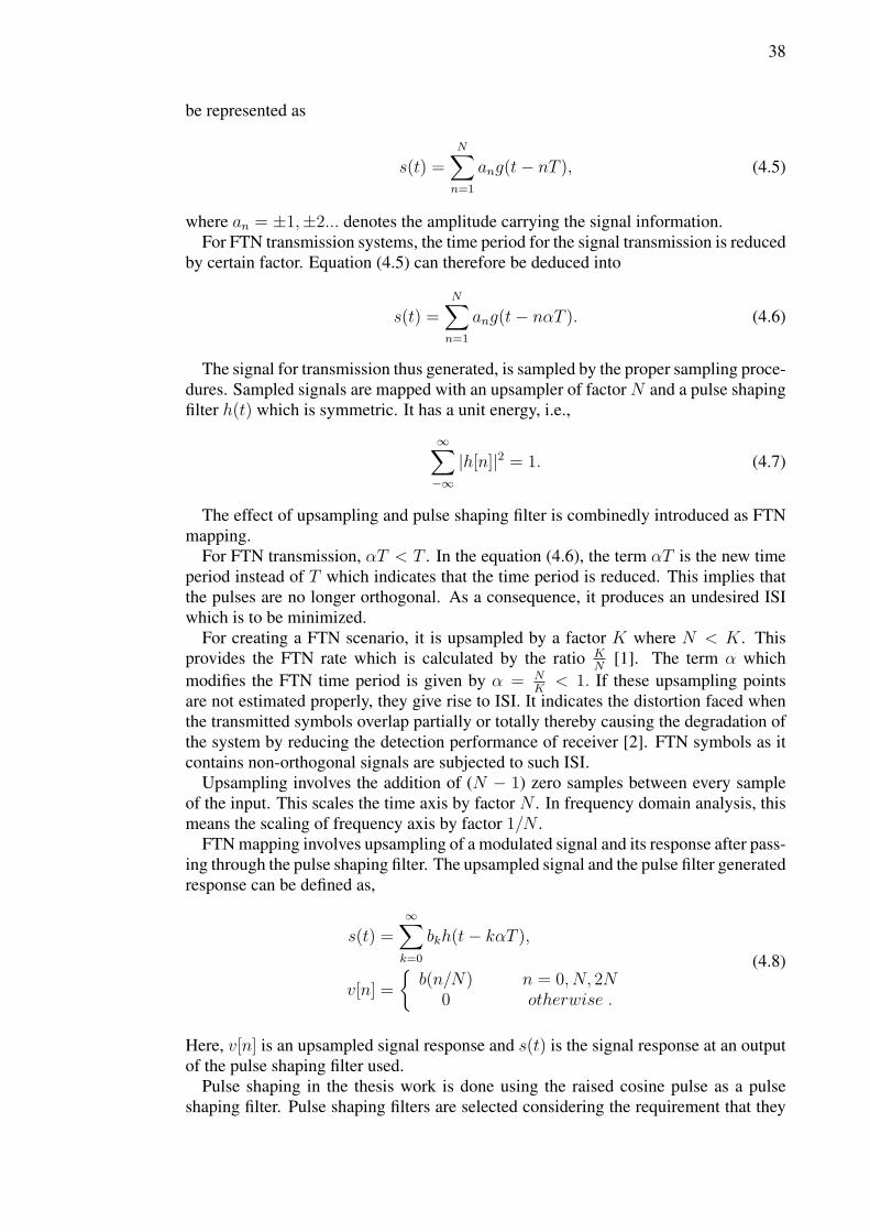
38

be represented as

s(t) =N∑n=1

ang(t− nT ), (4.5)

where an = ±1,±2... denotes the amplitude carrying the signal information.For FTN transmission systems, the time period for the signal transmission is reduced

by certain factor. Equation (4.5) can therefore be deduced into

s(t) =N∑n=1

ang(t− nαT ). (4.6)

The signal for transmission thus generated, is sampled by the proper sampling proce-dures. Sampled signals are mapped with an upsampler of factor N and a pulse shapingfilter h(t) which is symmetric. It has a unit energy, i.e.,

∞∑−∞

|h[n]|2 = 1. (4.7)

The effect of upsampling and pulse shaping filter is combinedly introduced as FTNmapping.

For FTN transmission, αT < T . In the equation (4.6), the term αT is the new timeperiod instead of T which indicates that the time period is reduced. This implies thatthe pulses are no longer orthogonal. As a consequence, it produces an undesired ISIwhich is to be minimized.

For creating a FTN scenario, it is upsampled by a factor K where N < K. Thisprovides the FTN rate which is calculated by the ratio K

N[1]. The term α which

modifies the FTN time period is given by α = NK< 1. If these upsampling points

are not estimated properly, they give rise to ISI. It indicates the distortion faced whenthe transmitted symbols overlap partially or totally thereby causing the degradation ofthe system by reducing the detection performance of receiver [2]. FTN symbols as itcontains non-orthogonal signals are subjected to such ISI.

Upsampling involves the addition of (N − 1) zero samples between every sampleof the input. This scales the time axis by factor N . In frequency domain analysis, thismeans the scaling of frequency axis by factor 1/N .

FTN mapping involves upsampling of a modulated signal and its response after pass-ing through the pulse shaping filter. The upsampled signal and the pulse filter generatedresponse can be defined as,

s(t) =∞∑k=0

bkh(t− kαT ),

v[n] =

{b(n/N) n = 0, N, 2N

0 otherwise .

(4.8)

Here, v[n] is an upsampled signal response and s(t) is the signal response at an outputof the pulse shaping filter used.

Pulse shaping in the thesis work is done using the raised cosine pulse as a pulseshaping filter. Pulse shaping filters are selected considering the requirement that they

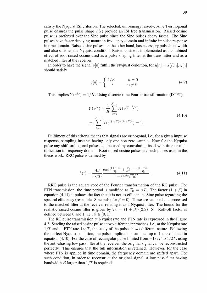
39

satisfy the Nyquist ISI criterion. The selected, unit-energy raised-cosine T-orthogonalpulse ensures the pulse shape h(t) provide an ISI free transmission. Raised cosinepulse is preferred over the Sinc pulse since the Sinc pulses decay faster. The Sincpulses have faster decaying nature in frequency domain and infinite impulse responsein time domain. Raise cosine pulses, on the other hand, has necessary pulse bandwidthand also satisfies the Nyquist condition. Raised cosine is implemented as a combinedeffect of root raised cosine used as a pulse shaping filter at the transmitter and as amatched filter at the receiver.

In order to have the signal y[n] fulfill the Nyquist condition, for y[n] = x[Kn], y[n]should satisfy

y[n] =

{1/K n = 0

0 n 6= 0.(4.9)

This implies Y (ejω) = 1/K. Using discrete time Fourier transformation (DTFT),

Y (ejω) =1

K

K−1∑k=0

X(ejωk− 2πKk)

or,K−1∑k=0

X(e(jω/K)−(2π/K)k) = 1.

(4.10)

Fulfilment of this criteria means that signals are orthogonal, i.e., for a given impulseresponse, sampling instants having only one non zero sample. Now for the Nyquistpulse any shift orthogonal pulses can be used by convoluting itself with time or mul-tiplication in frequency domain. Root raised cosine pulses are such pulses used in thethesis work. RRC pulse is defined by

h(t) =4β

π√T0

cos (1+β)πtT0

+ T04βt

sin (1−β)πtT0

1− (4βt/T0)2. (4.11)

RRC pulse is the square root of the Fourier transformation of the RC pulse. ForFTN transmission, the time period is modified as T0 = αT . The factor (1 + β) inequation (4.11) stipulates the fact that it is not as efficient as Sinc pulse regarding thespectral efficiency (resembles Sinc pulse for β = 0). These are sampled and processedto the matched filter at the receiver relating it as a Nyquist filter. The bound for therealistic raised cosine filter is given by T0 = (1 + β)/(2B) [5]. Roll-off factor isdefined between 0 and 1, i.e., β ∈ (0, 1).

The RC pulse transmission at Nyquist rate and FTN rate is expressed in the Figure4.3. Sending the raised cosine pulse at two different approaches, i.e., at the Nyquist rate1/T and at FTN rate 1/αT , the study of the pulse shows different nature. Followingthe perfect Nyquist condition, the pulse amplitude is summed up to 1 as explained inequation (4.10). For the case of rectangular pulse limited from −1/2T to 1/2T , usingthe anti-aliasing low pass filter at the receiver, the original signal can be reconstructedperfectly. This ensures that the full information is retained. However, for the casewhere FTN is applied in time domain, the frequency domain are shifted apart. Forsuch condition, in order to reconstruct the original signal, a low pass filter havingbandwidth B larger than 1/T is required.

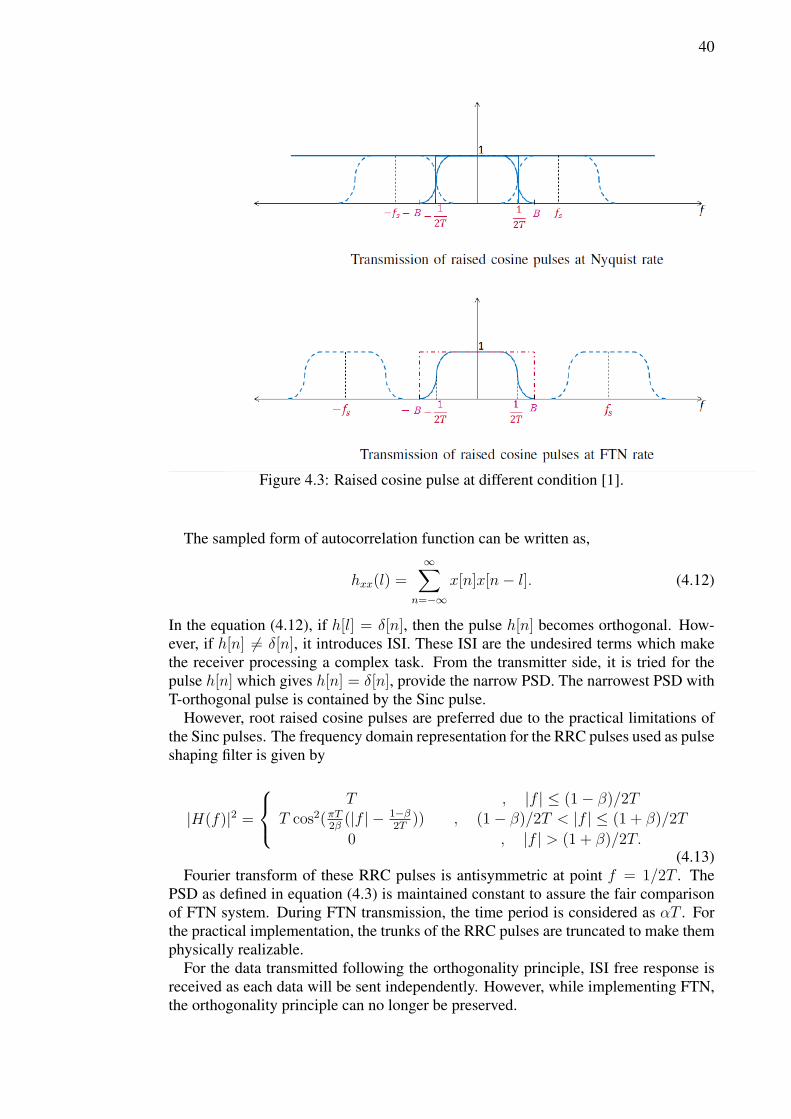
40

Figure 4.3: Raised cosine pulse at different condition [1].

The sampled form of autocorrelation function can be written as,

hxx(l) =∞∑

n=−∞

x[n]x[n− l]. (4.12)

In the equation (4.12), if h[l] = δ[n], then the pulse h[n] becomes orthogonal. How-ever, if h[n] 6= δ[n], it introduces ISI. These ISI are the undesired terms which makethe receiver processing a complex task. From the transmitter side, it is tried for thepulse h[n] which gives h[n] = δ[n], provide the narrow PSD. The narrowest PSD withT-orthogonal pulse is contained by the Sinc pulse.

However, root raised cosine pulses are preferred due to the practical limitations ofthe Sinc pulses. The frequency domain representation for the RRC pulses used as pulseshaping filter is given by

|H(f)|2 =

T , |f | ≤ (1− β)/2T

T cos2(πT2β

(|f | − 1−β2T

)) , (1− β)/2T < |f | ≤ (1 + β)/2T

0 , |f | > (1 + β)/2T.(4.13)

Fourier transform of these RRC pulses is antisymmetric at point f = 1/2T . ThePSD as defined in equation (4.3) is maintained constant to assure the fair comparisonof FTN system. During FTN transmission, the time period is considered as αT . Forthe practical implementation, the trunks of the RRC pulses are truncated to make themphysically realizable.

For the data transmitted following the orthogonality principle, ISI free response isreceived as each data will be sent independently. However, while implementing FTN,the orthogonality principle can no longer be preserved.

41

4.1.1.1. Normalization of energy

In FTN, the data pulses are transmitted in a compact form, i.e., more symbols aresent for the given time period. Comparatively, more samples/symbol are sent. Thissituation may require to increase the transmitted symbol power. However, to makesure of the fair comparison of FTN signaling, instead of increasing the power, pulseenergy is normalized making the power constant.

4.1.2. Receiver Design for FTN with MMSE equalizer

Now considering the AWGN channel, for the estimation of the information sequencean, the following expression describes the received signal y(t) such that

y(t) = sn(t) + n(t). (4.14)

Output sequence r(t) thus can be expressed as,

r(t) =

∫ ∞−∞

y(t)h∗(t− nαT )dt. (4.15)

The above equation (4.15) can be represented in a matrix notation as

rN = GNaN + ηN . (4.16)

Here GN represents N × N toeplitz matrix defined by {g[0], g[1], ....g[N − 1]}, aNrepresents {a[0], a[1], ....a[N − 1]}T and η represents the colored gaussian noise.

Here,

g[k] =

∫ ∞−∞|H(f)|2ej2πkαTfdf. (4.17)

The term ej2πkαTf is periodic and the term 1/αT is the multiple of period. The termg[k] can then be deduced as,

g[k] =∞∑

k=−∞

∫ 1/2αT

−1/2αT

|H(f + k/αT )|2ej2πkαTfdf. (4.18)

Now rearranging the summation and integral operation, we get,

g[k] =

∫ 1/2αT

−1/2αT

∞∑k=−∞

|H(f + k/αT )|2ej2πkαTfdf

=

∫ 1/2αT

−1/2αT

|Hfold(f)|2ej2πkαTfdf .(4.19)

The folded spectrum |Hfold(f)|2 is considered zero outside the interval −1/2αT ≤f ≤ 1/2αT , i.e.,

|Hfold(f)|2 =∞∑

k=−∞

|H(f + k/αT )|2, −1

2αT≤ f ≤ −1

2αT. (4.20)

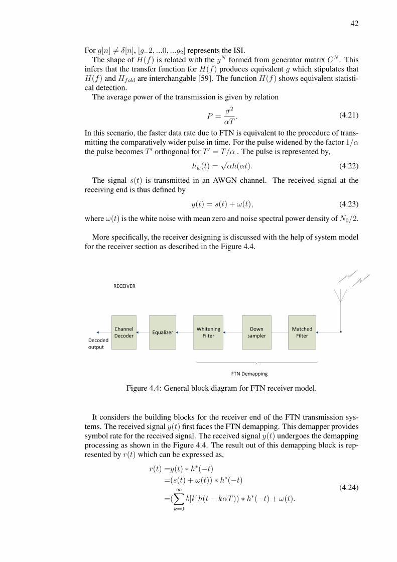
42

For g[n] 6= δ[n], [g−2, ...0, ...g2] represents the ISI.The shape of H(f) is related with the yN formed from generator matrix GN . This

infers that the transfer function for H(f) produces equivalent g which stipulates thatH(f) and Hfold are interchangable [59]. The function H(f) shows equivalent statisti-cal detection.

The average power of the transmission is given by relation

P =σ2

αT. (4.21)

In this scenario, the faster data rate due to FTN is equivalent to the procedure of trans-mitting the comparatively wider pulse in time. For the pulse widened by the factor 1/αthe pulse becomes T ′ orthogonal for T ′ = T/α . The pulse is represented by,

hw(t) =√αh(αt). (4.22)

The signal s(t) is transmitted in an AWGN channel. The received signal at thereceiving end is thus defined by

y(t) = s(t) + ω(t), (4.23)

where ω(t) is the white noise with mean zero and noise spectral power density ofN0/2.

More specifically, the receiver designing is discussed with the help of system modelfor the receiver section as described in the Figure 4.4.

RECEIVER

Matched Filter

Downsampler

Whitening Filter

EqualizerChannelDecoder

FTN Demapping

Decodedoutput

Figure 4.4: General block diagram for FTN receiver model.

It considers the building blocks for the receiver end of the FTN transmission sys-tems. The received signal y(t) first faces the FTN demapping. This demapper providessymbol rate for the received signal. The received signal y(t) undergoes the demappingprocessing as shown in the Figure 4.4. The result out of this demapping block is rep-resented by r(t) which can be expressed as,

r(t) =y(t) ∗ h∗(−t)=(s(t) + ω(t)) ∗ h∗(−t)

=(∞∑k=0

b[k]h(t− kαT )) ∗ h∗(−t) + ω(t).

(4.24)

43

The signal is sampled for every αT . Using the same pulse shapes as that of thepulse shaping filter of the transmitter side, matched filtering h∗(−t) is carried out forthe received signal y(t). The resulting signal r(t) is then finally downsampled by thefactor N . Whitening filter is used to whiten the colored noise. In the equation (4.24),ω(t) is the colored noise. The FTN process creates the ISI which is dealt with equalizerto mitigate the effects of such unwanted ISI. The soft output bits are generated out ofthe equalizer which is passed to the channel decoder.

FTN demapper consists of matched filter, desampler and the whitening filter. Thesampled data is generated from the received continuous signal r(t). This is done inthe matched filtering process. In reference to the upsampler used at the transmitter,receiver involves downsampler. Downsampling involves the removal of zero samples(i.e., scaling of time axis) which indicates the scaling of frequency axis by factor N .Using shift orthogonal pulses, the received structure can be represented as

rn =(y(t), hT (t− nT ))

=(s(t), hT (t− nT ) + (ω(t), hT (t− nT )

=∑m

am(hT (t−mT ), hT (t− nT )︸ ︷︷ ︸an

+ηη.(4.25)

Here an represents the information signal amplitude. The matched filter is matchedwith the pulse h(t) and this is sampled at the rate 1/αT . The basic representation ofsignal flow in matched filter is shown in Figure 4.5. The term ηη represents randomindependent gaussian noise with variance N0/2. It can be simply represented by, r =a + η , where r is the received signal and η is the i.i.d. gaussian noise vector. Thecase is assumed to be for the ideal situation having unit energy pulses. However, forthe situation where varying input power is desired, it can be achieved by using squareroot of power, i.e.,

√P as r = a+ ση, where σ =

√N0/2P . The term σ2 denotes the

variance which is defined by the inverse of linear SNR, i.e.,

σ =√N0/2P

=10−SRN/20(dB).(4.26)

The sampled noise having smaller value of standard deviation implies that the sam-ples are near to the actual values thereby making the estimation more accurate.

Pulse shaping

FilterModulatedInput data

S(t)

Noise n(t)

Received signal y(t)

Matched filter

Samples (rn)

Figure 4.5: Block diagram showing signal processing with matched filter.

44

After the matched filtering, there comes a whitening filter. This receiver filter is alsomatched to h(t) and sampled at each αT . For the further discussion, for equation,

x = a ∗ g + η,

gk =

∫h(t)h(t+ kαT )dt, (4.27)

where g is the sampled autocorrelation function of h(t) and η is the colored gaussiannoise. The z transform for above equation (4.27) can be written as

x(Z) = A(Z)G(Z) +N(Z). (4.28)

Now using the spectral factorization of G(z) into v(z)v∗(1/z∗), the whitening fil-ter is constructed. This decorrelates the colored noise η. So the whitening filter1/v∗(1/z∗) is used. This gives the modified relation as

y = a ∗ v + ω, (4.29)

where ω is the white gaussian noise with variance N0/2.

4.1.2.1. Mean square error estimation

Initially, the probability of error is minimized. Estimate of x is determined to ensurelow error probability for the data y with sent data vector a, i.e., x is calculated for thereceived signal r(t) such that it minimizes

minxP (x 6= a|r(t)).

Here,

P (x 6= a|r(t)) = 1− P (x = a|r(t)).

This is equivalent to,

maxxP (x = a|r(t)).

Using the Baye’s rule,

P (a|y) =P (y|a)P (a)

P (y)

= argmaxaP (y|a)P (a)

P (y)

= argmaxaP (y|a).

(4.30)

Here P (a) and P (y) are independent of a. The likelihood is defined by P (y|a).Thus maximum likelihood estimation (MLE) defines the estimation giving minimumerror probability. So for the pulses with information sequence an of N independentpulses, there exists vector a that maximizes expression for each component near to y.This can be mathematically written as,

xn = minan(yn − an)2.

45

4.1.2.2. Minimun mean square error equalizaion

In case of FTN signaling, both the non white noise and the ISI are to be taken intoaccount for the receiver design. The whitening filters are therefore followed by theequalizers. FTN signaling makes use of the compact form of signals, i.e., they containcomparatively more symbols for the given time period T than the conventional orthog-onal systems. This yields the ISI. So the linear MMSE equalizers are implemented toget rid of this interference.

For the information symbol an, where n is the symbol index, modulated with lcoded information bits, the transmission is carried out through the T orthogonal pulseshaping filter h(t). Each symbol is convolved with the shaping filter h(t) and the signalis transmitted at the symbol interval T0 ≤ T . Pulse shaping is done using the RRCfilters. The average energy of the symbol is thus given by the relation, Es = E{|an|2}.The individual symbol is transmitted at the interval of αT , i.e., signaling rate equalsto 1/αT . In the relation, α is maintained less than 1 for FTN transmissions whichindicates the ratio of the symbols compact or the symbol packing ratio. For the caseof orthogonality, α = 1. This indicates that ISI does not exists. As α decreases, therate of transmission increases but at the cost of increased error, which needs to beequalized. The MMSE equalizers treat the data symbols as random variables havingmean and variance calculated from the a priori information.

For the information sequence transmitted at FTN transmission scheme, the receivedsignal under the assumption of AWGN noise is given by

y(t) =√Es∑n

sng(t− nT0) + η(t), (4.31)

where

g(t) =

∫h(α)h∗(α− t)dα and

n(t) =

∫n(α)h∗(α− t)dα .

Here sn is the information symbol, h(t) is the impulse response of shaping filter, n isthe symbol index, n(t) is the guassian distributed complex random variableCN(0, N0)with zero mean and variance N0, Es the average power for the transmitted symbolsand T0 = αT , where α is the symbol packing ratio. Now under the assumption ofperfect synchronization between the transmitter and receiver, the received signal forkth sampled signal is given by

yk = y(kT0)

=√Es∑n

sng(kT0 − nT0) + η(kT0)

=√Esskg(0) +

√Es∑n 6=k

g(kT0 − nT0) + η(kT0)

(4.32)

In the equation(4.32), the first term represents the symbol of interest and the secondterm refers to the ISI. If symbol packing ratio α = 1, then this second term would

46

disappear as it would be perfect Nyquist condition. Now, retaining the high normal-ized rate of FTN, we use frequency domain equalization technique to overcome thisunavoidable ISI. The efficient fast Fourier transform (FFT) used in FDE also aids inhandling the channel impulse response spread over large range of symbols. Since theuncoded FDE for the FTNs receiver does not meet the optimal performance, somecoding techniques can be beneficial.

It considers the implementation of finite-tap equalizers to compensate linear ISI inthe presence of additive white Gaussian noise. For the received signal rk and inputsequence estimate ak,

MSE = E[|rk − ak|2]. (4.33)

These equalizers de-convolves the linearly distorted channel along with the transver-sal filter in a way that it generates an inverse of the channel. The equalizer output isquantized to reconstruct the original transmitted symbols. The error estimation is givenby

e(k) = r(k)− ˆa(k).

Now the minimization of E|e[k]|2 is required.Finally the MMSE equation for linear filter in frequency domain is given by,

C(z) =H∗(z)

H(z)H∗(z) + σ2, (4.34)

where H(z) represents the pulse frequency response, * represents conjugate operationand σ2 is the noise variance.

Frequency domain equalization offers an advantage over its corresponding time do-main in the sense that fast convolution can be carried out in frequency domain reducingthe processing operations. Unlike the time domain where each tap weight is relatedto the entire set of channel impulse response for all delays, the frequency domainresponse of the equalizer is related with the channel response corresponding to thatparticular instant of frequency and its additional alias frequency. In addition to this,the frequency domain algorithms are faster and more stable [60].

4.1.3. Receiver design for FTN transmission with turbo coding

The high data rate due to FTN is possible at the cost of increased ISI. This situationstipulates the need of an efficient FTN equalizer at the receiving end. For the uncodedsystem, this increment in the rate due to FTN is directly related to lowering the valueof FTN time period α = T0/T . But at the same time, this creates the degradation ofthe BER performance of the system. For the BPSK modulation of the signals with rootraised cosine pulse as a pulse shaping filter, the FTN performance is scrutinized withMMSE equalization as explained in section 4.1.2.

In order to compensate this loss due to ISI, some channel coding techniques liketurbo codes, LDPC codes can be implemented. In this part of work, turbo codingis utilized and the performance is evaluated. Turbo coding makes use of an iterativedecoding of these error correcting codewords. The transmitter and receiver model isassumed considering an AWGN channel with the code rate r. The ISI effect which is

47

produced due to FTN transmission is mapped to a trellis structure and finally analyzedusing the iterative turbo decoder following BCJR algorithm.

These high-performance FEC codes have the performance much better than the cor-responding convolution code. The turbo codes makes use of RSC encoder and iterativeBCJR decoder. RSC turbo encoder contains the encoder and an interleaver.

At the transmitter side, the source coded data bits are passed through an encoderwhich produces encoded data bits. Turbo encoder used for the thesis work is with rate1/3. The pseudo random interleaver is used for generating the interleaved data bits.

RSC Encoder 1

RSC Encoder 2

Puncturing

Interleaver

Input Information bits

Systematic bits

Parity bits

Interleaved parity bits

Figure 4.6: Basic block of Turbo encoder with rate 1/3.

As seen in the Figure 4.6, the encoder consisting one input information of sequenceof lengthN and three output sequences is used. It has the coding rate 1/3. Input data isencoded to produce three different outputs as systematic, first parity and second paritysequences. In the thesis work, code rate of the turbo code is varied in order to analyzethe performance of the system at different conditions. This is done by the process ofpuncturing. Using the puncturing pattern to modify the encoded data, the code rate isincreased. To make the fair comparison during the result analysis, FTN rate and thecode rate is manipulated to make the overall rate equivalent at different situations.

The generator polynomial function for the encoder is defined by

G[D] =[1 1+D+D2

1+D2

]The encoder structure contains three different forms of encoder output. The first

encoder generates the parity bit from the input information bits. It is denoted by P0.Likewise, next encoder generates the parity bit P1. The interleaver used changes thepattern of the input and generates the interleaved version of the input data Xπ from X .

Mathematically, it is represented as,

X = X0X1...Xn−1

Xπ = X0πX

1π...X

n−1π .

(4.35)

48

It comprises of the information bits X(D) and the parity bits

X(D)1 +D +D2

1 +D2= P 0

0P10 ...P

N−10 and

Xπ(D)1 +D +D2

1 +D2= P 0

1P11 ...P

N−11 .

Now considering C0(D) = X(D) , C1(D) = X(D)1+D+D2

1+D2 , and F (D) = X(D)1+D2 ,

we get the relation,

Cj0 = Xj

Cj1 = Xj + F j−1.

(4.36)

In the above relation (4.36), F j = F (j−2) + Xj . The encoded code word from theencoder can therefore be given by,

C = X0P 00P

01 , X

1P 10P

11 , ...X

N−1PN−10 PN−1

1 . (4.37)

System model including the turbo code shows that the encoded data bits are passedthrough the modulator. The signals are BPSK modulated before they are finally passedinto the pulse shaping filter. The modulation in this case can be expressed as

uj0 = 2Xj − 1

uj1 = 2P j0 − 1

uj1 = 2P j1 − 1,

(4.38)

where j = 0, 1, 2...N − 1. Puncturing matrix is used as shown in the Figure 4.6to modify the encoded bits such that the code rate is increased. The number of bitstransmitted is reduced as compared to non punctured bits without reducing informationbits. This causes the rate to be increased. Puncturing matrix (P) used for changing thecode rate is given by,

P =

1 1 1

1 1 1

1 1 1

1 1 1

code rate 1/3

Ppunctured =

1 1 1

1 × 1

1 1 1

1 × ×

Punctured rate 4/9

In the matrix, × denotes the punctured bit.In the matrix P, the first column, second column and third column represents the

information bits, parity bits from first encoder and the interleaved parity bits respec-tively. The rate is thus defined as k/n = 4/12 = 1/3 , where k and n represents theinformation bits and the total (including information and parity) bits respectively. Nowusing the puncturing matrix Ppunctured, some parity bits are removed from the matrix inthe pattern as shown such that rate r changes to 4/9. Turbo code with changed rate is

49

created to make the fair comparison between the coded systems using FTN and codedNyquist satisfied scenarios. In the first case ,the turbo code with rate 1/3 is modifiedwith puncturing matrix to generate the code rate 4/9 and FTN rate 1 is used makingthe overall rate equal to 4/9. In the second case, turbo code with rate 1/3 and the FTNrate 8/6 is used making the same overall rate equal to 1

3× 8

6= 4/9. This provides an

environment for the fair comparison between the two approaches.At the receiving end, decoding of the received code words is performed. Received

signal in our case is the equalized output from the MMSE equalizer. It uses the BCJRalgorithm. The BCJR decoder architecture contains two decoders for the correspond-ing two encoders. The inputs for the decoder is represented by R0 and R1 for the firstdecoder and πR0 and R2 for second decoder, respectively.

The log aposteriori probability ratio(LAPPR) is thus defined as

Λk = logP (Xk = 1|R)

P (Xk = 0|R),

Λk1 = Λk − logP (Xk = 1)

P (Xk = 0)− 2Rk

0

σ2,

(4.39)

where R is the input to decoder and k = 0, 1, 2...N − 1.For the first BCJR decoder, the input is represented by R = R0 R1. We have the

relation,

P (Xk = i|R) =1

P (RN−10 )

M−1∑m=0

M−1∑m′=0

αk(m′)γik(m

′,m)βk(m). (4.40)

In the equation (4.40), m and m′ are stages (sk) , M is the total number of stagesand i = 0 or 1 (input). The terms αk(m′), βk(m) and γik(m

′,m) represents forwardstate metric, backward state metric, and transition probability from state m′ to m atstage k for input i, respectively, i.e.,

αk(m′) = P (Sk = m′|Rk−1

0 ) =M−1∑m′′=0

1∑i=0

γik−1(m′′,m)αk−1(m′′), (4.41)

βk(m) = P (RN−1K+1|Sk+1 = m) =

M−1∑m′=0

1∑i=0

γik+1(m′,m)βk+1(m′), (4.42)

γik(m′,m) =

P (Xk = i)︸ ︷︷ ︸Apriori probabilityat time k for input i

P (Sk+1 = m|Sk = m′, Xk = i)︸ ︷︷ ︸contribution from

trellis

P (Rk|Sk+1 = m′, Sk = m,Xk = i)︸ ︷︷ ︸contribution from

likelihood

.

(4.43)The equations (4.41), (4.42) and (4.43) in addition with the apriori probabilities for

inputs 0 and 1, is used to calculate the LAPPR for all stages and decoding of thecodewords. At all stages for both the inputs, the output from the first decoder is passed

50

to the second decoder. This helps to calculate the priory probability using LAPPRvalues. The process is continued iteratively until both the decoders have similar orthe priory probability is 1 for one of the input. The values of α, β, and γ is used todetermine the value of Λk for all the stages, i.e.,

P (Xk = 1) =eΛk1

1 + eΛk1,

P (Xk = 0) =1

1 + eΛk1.

(4.44)

The BCJR algorithm and the interleaver arrangements for the BCJR output standsfor the main role at the decoder. The algorithm computes the LAPPR for the convolu-tional code symbols which gives the aproiori probabilities of the symbol with respectto each other. The probabilities are produced in the form of series of iterations thatultimately converges for the LLR to represent the correct codeword [6].

In FTN, increase in the data rate is achieved at the cost of an unavoidable ISI whichimposed the processing difficulties. However, with the use of these FEC turbo codes,receiver processing is justified with the benefits of FTN gain added with some codinggains.

51

5. MATLAB IMPLEMENTATION AND SIMULATION RESULTS

This chapter concentrates about the simulation setup environment for the performanceanalysis of the FTN transmission system. The results are presented for two differentapproaches. Firstly, the FTN transmission results of an uncoded system is kept for-ward. Then the comparative study for the system introducing the coded transmissionis presented. The fair comparison of the coded system is ensured by providing thesame rate of transmission for the coded system under usual Nyquist conditions andFTN transmission systems. As stated in [61], FDE provides lower complexity thanits corresponding time domain equalization. Therefore, the receiver designing task isimplemented utilizing the frequency domain characteristics.

5.1. FTN analysis under an uncoded system

The uncoded binary modulated signals are transmitted as an information bearing sig-nals. These signals are designed in a way that they are transmitted at a rate faster thanthe rate prescribed by Nyquist criterion by introducing some oversampling factors.The upsampled signals thus created during FTN mapping defines the FTN scenario.These signals are introduced to FTN environment by using an upsampler of factor Nand upsampled by the factor K, where N < K. The ratio N

Kdefines the FTN rate.

The signals are then introduced to pulse shaping filter. The Nyquist condition satisfy-ing root raised cosine pulse is used to shape the modulated signal before transmission.The pulses are ensured that they really meet the Nyquist criteria. At the receivingend, the received signals are matched using the matched filter which is addressed withthe corresponding down sampling procedures as reference to the up sampled signals.ISI free property of RC pulse comes after implementing the combined effect of RRCpulses as a pulse shaping filter at transmitter and as a matched filter at the receiver.The whitening filters are used to mitigate the effects of the colored noise. Finally, theMMSE equalizer is used to equalize the received signals. These equalized resultingsignals are then compared with the original transmitted signals. The BER calculationof the signals is used to analyze the system performance.

5.1.1. Results

The MATLAB simulation plots are presented to analyze the results at different con-dition of FTN signaling. In the simulation results, alpha (α) denotes the FTN factorwhere symbol duration T is reduced to αT , α ≤ 1. For α = 1, it represents thescenario satisfying Nyquist condition.

52

0 2 4 6 8 10 12 1410

−8

10−7

10−6

10−5

10−4

10−3

10−2

10−1

100

SNR (dB)

BE

R

FTN response with Equalization

MMSE ResponseMF ResponseMMSE ResponseMF Response

alpha = 1

alpha = 0.8

Figure 5.1: Comparison for Nyquist and FTN response with MMSE equalizer.

Figure 5.1 contains the plots for normal Nyquist condition satisfying transmissionand the introduction of FTN signaling with FTN factor (α) = 0.87. For α = 1, theNyquist signaling shows that MMSE equalizer response and matched filter (MF) re-sponse are equivalent. This indicates that equalizer has no significant role for suchtransmissions as there occurs no ISI since the signals are perfectly orthogonal. Thesignal degradation for the case with α = 0.87 is due to the generation of ISI which iscreated as a consequence of FTN signaling as FTN makes the signal non orthogonal.In this case, equalizer has the dominant effect. MMSE equalizer mitigates an effect ofISI, therefore shows an improvement over the MF output.

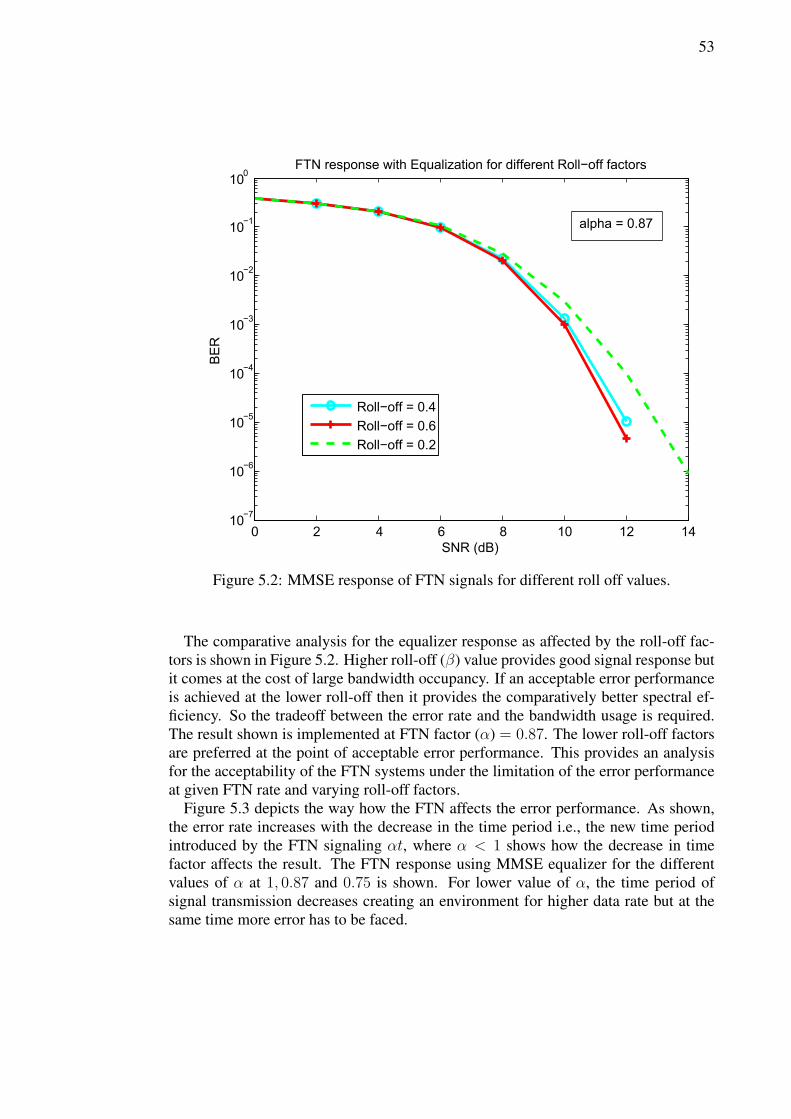
53

0 2 4 6 8 10 12 1410

−7

10−6

10−5

10−4

10−3

10−2

10−1

100

SNR (dB)

BE

R

FTN response with Equalization for different Roll−off factors

Roll−off = 0.4Roll−off = 0.6Roll−off = 0.2

alpha = 0.87

Figure 5.2: MMSE response of FTN signals for different roll off values.

The comparative analysis for the equalizer response as affected by the roll-off fac-tors is shown in Figure 5.2. Higher roll-off (β) value provides good signal response butit comes at the cost of large bandwidth occupancy. If an acceptable error performanceis achieved at the lower roll-off then it provides the comparatively better spectral ef-ficiency. So the tradeoff between the error rate and the bandwidth usage is required.The result shown is implemented at FTN factor (α) = 0.87. The lower roll-off factorsare preferred at the point of acceptable error performance. This provides an analysisfor the acceptability of the FTN systems under the limitation of the error performanceat given FTN rate and varying roll-off factors.

Figure 5.3 depicts the way how the FTN affects the error performance. As shown,the error rate increases with the decrease in the time period i.e., the new time periodintroduced by the FTN signaling αt, where α < 1 shows how the decrease in timefactor affects the result. The FTN response using MMSE equalizer for the differentvalues of α at 1, 0.87 and 0.75 is shown. For lower value of α, the time period ofsignal transmission decreases creating an environment for higher data rate but at thesame time more error has to be faced.

54

0 2 4 6 8 10 12 14 1610

−6

10−5

10−4

10−3

10−2

10−1

100

SNR (dB)

BE

R

MMSE responses at different FTN scenarios

alpha=1alpha=0.87alpha=0.75

Figure 5.3: MMSE response of FTN signals at different α values.

0 2 4 6 8 10 12 14 16 18 2010

−8

10−7

10−6

10−5

10−4

10−3

10−2

10−1

100

SNR (dB)

BE

R

FTN Response with Equalization

MMSE ResponseMF ResponseMMSE ResponseMF Response

alpha= 0.75

alpha= 0.87

Figure 5.4: Comparative analysis of MMSE and MF response of FTN signals.

55

0 2 4 6 8 10 12 1410

−8

10−7

10−6

10−5

10−4

10−3

10−2

10−1

100

SNR (dB)

BE

R

FTN response with Equalization

MMSE ResponseMF ResponseMMSE ResponseMF Response

alpha = 1

alpha = 0.8

Figure 5.5: Comparative analysis of MMSE and MF response of FTN signals.

Varying the time period or the symbol packing ratio (FTN factor), the variation inthe signal response is observed. The comparative high error rate for less time period isdue to the generation of ISI. Lesser the time factor, more is the error. This is due to theincrement of the non orthogonality behavior of the signals. The different approachesfor FTN at α = 1, 0.87 and 0.75 is shown. Figure 5.4 shows the comparative analysis ofMMSE equalizer response and matched filter response at α = 0.87 and 0.75. Likewise,Figure 5.5 shows the response at α = 1 and 0.87. Equalizer effect is more significantfor the system with reduced time period since the ISI is more notable in such case.

5.2. FTN analysis under Turbo coded system

In the thesis work, turbo code implementation is performed as the next approach toanalyze the performance measure under the coded system. The binary modulated sig-nals are encoded with the turbo encoder. Evaluation of turbo codes is measured interms of BER. AWGN channel model is used for simplicity. Decoder performs iter-ative processing to ensure the acceptable error performance. Though the increase inthe number of iterations improve the turbo code performance but after certain point noany significant improvement is observed thereby showing similar BER. So the itera-tion loop is fixed such that extra computational load is avoided. In the simulation, withBCJR decoding algorithm, it is observed that the BER decreases after each iteration,however after the fourth iteration, no further improvement is seen. The time require-

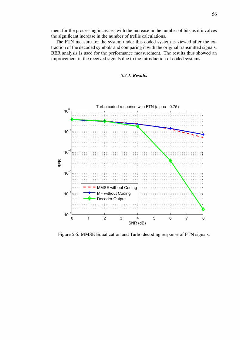
56

ment for the processing increases with the increase in the number of bits as it involvesthe significant increase in the number of trellis calculations.

The FTN measure for the system under this coded system is viewed after the ex-traction of the decoded symbols and comparing it with the original transmitted signals.BER analysis is used for the performance measurement. The results thus showed animprovement in the received signals due to the introduction of coded systems.

5.2.1. Results

0 1 2 3 4 5 6 7 810

−5

10−4

10−3

10−2

10−1

100

SNR (dB)

BE

R

Turbo coded response with FTN (alpha= 0.75)

MMSE without CodingMF without CodingDecoder Output

Figure 5.6: MMSE Equalization and Turbo decoding response of FTN signals.

57

0 1 2 3 4 5 6 7 810

−5

10−4

10−3

10−2

10−1

100

SNR (dB)

BE

R

Turbo coded response with FTN (alpha= 0.87)

MMSE without CodingMF without CodingDecoder Output

Figure 5.7: MMSE Equalization and Turbo decoding response of FTN signals.

0 1 2 3 4 5 6 7 810

−5

10−4

10−3

10−2

10−1

100

SNR (dB)

BE

R

Turbo coded response with FTN (alpha= 1)

MMSE without CodingMF without CodingDecoder Output

Figure 5.8: MMSE Equalization and Turbo decoding response of FTN signals.

58

The Figures 5.6, 5.7 and 5.8 demonstrate the comparative study of the simulatedresults for MF, equalizer output and the decoded results at α = 0.75, 0, 87 and 1 re-spectively. The simulations are performed keeping the roll-off factor equal to 0.4 andthe individual results for different FTN time factors are demonstrated. The increasein error rate for corresponding decrease in symbol duration is due to the non orthog-onal signals, hence more interferences. For less time period, this non orthogonalitybehaviour of the transmitting signals are comparatively higher thereby creating moreinterferences. Equalizers are responsible for mitigating the ISI effect. The decoder areused such that they can correct the errors in the equalized symbol sequences. Turbocode implementation is carried out for lower SNR values compared to previous com-parison of equalizer result at higher SNRs as they show good BER effects with lowerSNR. For high SNR, decoding results are almost optimal due to the low weight code-words.

0 1 2 3 4 5 6 7 810

−5

10−4

10−3

10−2

10−1

100

SNR (dB)

BE

R

Decoded output at different FTN scenarios

alpha= 0.75alpha= 0.87alpha= 1

Figure 5.9: Turbo coded response for FTN signals at different α values.

Figure 5.9 shows the advantage of turbo coding output for the FTN transmittedsignals. It shows the comparative analysis of the FTN signals as a decoded output atdifferent FTN values. Results for decoded output at α = 0.75, 0, 87 and 1 is shown.The error rate is significantly decreased at first and at the later stage it does not showdistinct change for high SNR. The peculiarity seen in the graph is due to the error floor.It is seen that the BER curve falls off sharply with increasing SNR for the moderateerror rates. Then the curve starts flattening at high SNR. So it is recommended to

59

execute the BER simulation at lower values. This situation is referred as error floor.In fact this error floor inhibits the turbo code performance to achieve extremely lowerror rates. The low weight code words are responsible for this error floor [62]. Thesituation is more significant in high order SNRs.

0 1 2 3 4 5 6 7 8 9

10−5

10−4

10−3

10−2

Turbo decoder performance over AWGN channel for BPSK modulated symbols

SNR (dB)

BE

R

Punctured OutputUnpunctured Output

Figure 5.10: Comparative responses for Punctured and Unpunctured Turbo codes.

Simulated plots for the turbo encoded and iteratively decoded with BCJR decodingalgorithm is presented in Figure 5.10. It contains the plots with code rates 1/3 and4/9. At first the plot for code rate 1/3 is generated. Then, the code is punctured tochange the code rate. Using the puncturing matrix as shown in section 4.1.3 the coderate is changed to 4/9. Puncturing increases the code rate as it allows the informationto be transmitted with comparatively less number of bits than unpunctured code but atthe same time BER is increased due to the reduction in the number of parity bits.

60

0 1 2 3 4 5 6 7 8 9

10−5

10−4

10−3

10−2

10−1

SNR(dB)

BE

R

Comparison of Turbo decoded response and FTN response at Equivalent rate

FTN OutputTurbo Output

alpha= 0.75

Figure 5.11: Comparative analysis making the rate equivalent for FTN and Turbocoding.

For the comparative study of FTN transmission under coding systems, the compari-son is made at equivalent scenario for the rate. In Figure 5.11, first the turbo code withcode rate 4/9 is drawn. This is done by puncturing the 1/3 code rate with puncturingmatrix. This is carried out with FTN rate 1. For the next result the turbo code of rate1/3 and the FTN rate 8/6 is processed to view the result. Then the comparison of thesystem due to this coded response with the uncoded system is justified as the overallcondition provided a fair comparison for both the cases with same rate 4/9. The resultfor two approaches is presented in the graph which showed that the FTN benefits comeat the cost of increased error rate.

61

6. DISCUSSION AND FUTURE SCOPE

Considering the limited bandwidth resources availability for the future wireless com-munications systems, the thesis work is focused to address the issue by discussing anidea to attain high data rates without decreasing the spectral efficiency. The nobleapproach to use the non orthogonal pulses to reduce the symbol duration such thatmore data are transmitted at the given time with same spectral efficiency and errorrate performance as that of orthogonal transmission systems is considered as the FTNsystems.

Extending the traditional Nyquist transmission criteria for ISI free scenario to thenew approach of faster data speed attainment is explored. The FTN process was intro-duced by modulating the pulses faster than the Nyquist rate. Taking into account of theMazo [3] explanation of FTN signaling for the Sinc pulses, further modification is car-ried out. In Mazo [3], it is explained that using binary antipodal modulation, the incre-ment in the modulation rate by 25% has no effect on the minimum euclidean distancebetween the closest signals. This stipulates the fact that the FTN induced transmis-sion systems helps to increase the transmission speed without increasing bandwidthconsumption. In short, it increases the bit rate and preserves the signal bandwidth.However, producing the ISI as a consequence builds an additional burden at the re-ceiver processing. The ways to deal with this ISI is evaluated for both the coded anduncoded systems.

FTN transmission is dedicated to build an approach to transmit maximum data uti-lizing the minimum bandwidth possible such that it can be ensured that larger numberof subscribers are possible within the given constraints. Thesis task is scrutinized fortwo different approaches. The coded and uncoded data bits are used for signal trans-mission separately and the results were investigated. System design included turbocoding systems to encode the data before modulation are given the appropriate pulseshaping. Modulation helps to improve the system performance by matching the infor-mation signal characteristics to those of the channel characteristics. Relevant selectionof shaping filters and roll-off factors also showed great impact on the received sig-nal accuracy. With the decrease in the value of roll-off factor, the spectral efficiencyof the RRC pulses decrease monotonically [63]. Regarding the use of turbo encoder,the interleaver pattern and the concatenation pattern of the RSC encoders play an im-portant role for increasing the efficiency. Using the puncturing techniques, code ratewas changed and the comparison of the FTN coded and uncoded systems were mademaking the total rates equivalent for both the systems.

Thesis provides an approach to simplify the receiver processing techniques. Majorissue comes to balance between throughput and complexity. Advantage of the FTN isdiscussed regarding this matter. The PSD is fixed but bit density in bits/Hz-s is higherthan traditional Nyquist signaling. Since it can be inferred that the main task of FTNcomplexity lies at the receiver end to tackle the demodulating complexity, FTN can bethe suitable approach for the uplink of a cellular network where the complexity is moreat the base stations. This builds an approach to serve the high-end devices like smartphones, smart vehicles etc., in downlink. Since FTN can provide more data densitywithout increasing signal power, they can also be a good approach for future satelliteand mobile communication systems.

Thesis highlights the system that combines equalization with coded modulation.Matching the transmitter and receiver filters provide the optimum BER performance.MMSE equalizer is used to overcome the ISI and also the colored noise due to FTN.

62

Turbo codes are considered as a high performance error correcting codes close to Shan-non limit. Statistical measures like posteriori probability and likelihood were studiedto analyze the error performance with BCJR decoding algorithm. Using an iterativedecoding process to these soft output, performance is improved. Thus the frequencydomain equalization of the MMSE equalizer and the iterative decoding algorithm ofthe turbo decoder are implemented to achieve the explicit benefit eliminating the in-terferences. The simulation result proposes the benefits of using FTN system with lowcomplexity receiver and better BER proficiency over conventional Nyquist transmis-sion systems.

6.0.2. Future Studies

More powerful codes can be used to increase the throughput with the benefit of cod-ing gains and also the optimization of the pulse signals used can be a better approachto improve the performance [64]. Moreover, higher order modulation and their effectregarding distortion sensitivity and error rate, throughput, complexity etc., on FTNsystem is an interesting topic [65]. Study can be further extended to improve the ca-pacity of the system in the bandwidth starved scenario. FTN researches has led tothe achievement of higher Shannon capacity and creating new capacity attributes [6].FTN implementation in the OFDM systems and also the research over filter bank mul-ticarrier (FBMC) is another interesting topic which is expected to overrule the existingadvantages of the contemporary systems. The combination of FTN and MIMO tech-niques can be considered to generate new interest areas for future wireless commu-nications. The peak average power ratio (PAPR) evaluation of FTN and the possibleways to overcome it can make it an interesting research field.

Due to the complicated receiver structure, it might be considered as a complexmeans to be used in future networks. However, with the improvements in receiverprocessing complications, this approach of FTN signaling can be forwarded as a goodalternative to address the issue of high speed transmission requirement.

63

7. SUMMARY

The thesis work involves the study of the signal transmission and its effect when thetransmission procedures are carried out going beyond the Nyquist ISI criteria. Sig-nals are transmitted at the rate faster than the signaling rate recommended by Nyquistcriteria and the results under these circumstances are scrutinized.

The FTN scheme is used as a modification over the ordinary linear modulationthereby creating a scenario where higher data rates are achieved. The receiver pro-cessing techniques explained in the thesis work makes this practically realizable. Per-formance results for both the coded and the uncoded systems prove the improvementover this ordinary modulation technique compared over the identical situation of bitenergy, spectrum and error rate. The proposed scheme for the receiver designing withthe FDE based MMSE equalizer and the iterative decoding of the received data bitswith the turbo coding approach is presented. This simplifies the receiver decodingcomplexity. The iterative decoding used in the turbo decoder structure showed thecomparative improvement in the system performance. Simulation results highlight theadvantage of FTN implementation in the signal transmission process. Error rate of anorthogonal transmission system is achieved nearly even with the non orthogonal sig-nal usage. To achieve the more data rate for the given bit energy, and the error rate,the FTN signals makes use of the excess pulse bandwidth for the signal transmissionwhich ultimately ends up in less bandwidth consumption. This created an opportunitythat more symbols could be transmitted at the given time period. FTN implementationis therefore the promising approach to help achieve the higher data rates at the cost ofsame bandwidth consumption, bit energy and error rate as that of Nyquist transmis-sion. In FTN, the signals are no longer orthogonal with respect to symbol time. Usingthe non orthogonal pulses as the pulse signal is the key aspect to improve the speed.FTN factor represents the speed factor. Different FTN factors yield different results.Less the value of this FTN factor, higher is the speed of transmission. This is viewedfrom frequency domain aspect as the squeezing of the more signals together. The ISIwhich acts as a dominant limiting factor, occurred due to such non orthogonal pulsesare minimized with the use of MMSE equalization method and the iterative approachof BCJR decoding algorithm.

The analysis of the simulation results for both coded and uncoded signal transmis-sion schemes emphasize the importance of FTN signaling to be used in the futurewireless communication systems.

64

BIBLIOGRAPHY

[1] El Hefnawy M. & Taoka H. (2013) Overview of Faster-than-Nyquist for fu-ture mobile communication systems. In: Vehicular Technology Conference (VTCSpring), 2013 IEEE 77th, IEEE, pp. 1–5.

[2] Proakis J.G. (1995) Digital communications. New York ; Singapore : McGraw-Hill, third edition.

[3] Mazo J. (1975) Faster-than-Nyquist signaling. The Bell System Technical Journal54, pp. 1451–1462.

[4] Rusek F. & Anderson J.B. (2008) Non binary and precoded faster than Nyquistsignaling. IEEE Transactions on Communications 56, pp. 808–817.

[5] Sugiura S. (2013) Frequency-Domain Equalization of Faster-than-Nyquist Sig-naling .

[6] Anderson J.B., Rusek F. & Owall V. (2013) Faster-than-Nyquist signaling. Pro-ceedings of the IEEE 101, pp. 1817–1830.

[7] Tomoki S. & Adachi F. (2003) Comparative study of various frequency equaliza-tion techniques for downlink of a wireless OFDM-CDMA system. IEICE trans-actions on communications 86, pp. 352–364.

[8] Berrou C., Glavieux A. & Thitimajshima P. (May 1993) Near Shannon limiterror-correcting coding and decoding: Turbo-codes.1,. In: Technical Program,Conference Record, IEEE International Conference on Communications, ICC’93 Geneva,, volume 2, pp. 1064–1070.

[9] Decoding S.I. (2005) Transactions Letters. IEEE Transactions on Communica-tions 53, pp. 209.

[10] Divsalar D. & Pollara F. (1995) Multiple turbo codes for deep-space communi-cations .

[11] Patel S., Chauhan M. & Kapadiya K. (2012) 5G: Future mobile technology-vision 2020. International Journal of Computer Applications 54.

[12] Monserrat J.F., Droste H., Bulakci O., Eichinger J., Queseth O., Stamatelatos M.,Tullberg H., Venkatkumar V., Zimmermann G., Dotsch U. et al. (2014) Rethink-ing the mobile and wireless network architecture: The METIS research into 5G.In: European Conference on Networks and Communications (EuCNC), 2014,IEEE, pp. 1–5.

[13] Sharma P. (2013) Evolution of mobile wireless communication networks-1G to5G as well as future prospective of next generation communication network. In-ternational Journal of Computer Science and Mobile Computing 2, pp. 47–53.

[14] Li Q., Niu H., Papathanassiou A. & Wu G. (2014) 5G network capacity: Keyelements and technologies. Vehicular Technology Magazine, IEEE 9, pp. 71–78.

65

[15] Haider F., Gao X., You X.H., Yang Y., Yuan D., Aggoune H.M. & Haas H. (2014)Cellular architecture and key technologies for 5G wireless communication net-works. IEEE Communications Magazine p. 123.

[16] Tudzarov A. & Janevski T. (2011) Functional architecture for 5G mobile net-works. International Journal of Advanced Science and Technology 32, pp. 65–78.

[17] Patil S., Patil V. & Bhat P. (2012) A review on 5G technology. International Jour-nal of Engineering and Innovative Technology (IJEIT) 1, pp. 26–30.

[18] Osseiran A., Boccardi F., Braun V., Kusume K., Marsch P., Maternia M., Que-seth O., Schellmann M., Schotten H., Taoka H. et al. (2014) Scenarios for 5Gmobile and wireless communications: the vision of the METIS project. IEEECommunications Magazine 52, pp. 26–35.

[19] Soldani D. & Manzalini A. (2014) A 5G Infrastructure for Anything-as-a-Service. Journal of Telecommunications System & Management pp. 2167–0919.

[20] Sapakal M.R.S. & Kadam M.S.S. (2013) 5G Mobile Technology. InternationalJournal of Advanced Research in Computer Engineering & Technology 2.

[21] Huawei (2013) A 5G technology vision. Technical report, Huawei TechnologiesCo., Ltd.

[22] Nyquist H. (1928) Abridgment of certain topics in telegraph transmission theory.Journal of the AIEE, 47, pp. 214–217.

[23] Oshana R. (2006) DSP Software Development Techniques for Embedded andReal-Time Systems. Embedded Technology, Elsevier Science.

[24] Nyquist H. (1928) Certain topics in telegraph transmission theory. Transactionsof the American Institute of Electrical Engineers, 47, pp. 617–644.

[25] Kang A. & Sharma V. (2011) Pulse Shape Filtering in Wireless Communication-A Critical Analysis. Pulse 2.

[26] KavehPahlavan A.H.L. (2005) Wireless Information Networks. In: Wireless In-formation Networks, John Wiley and Sons.

[27] Wu Z., Zhu F. & Nassar C.R. (2002) Ultra wideband time hopping systems:performance and throughput enhancement via frequency domain processing. In:Conference Record of the Thirty-Sixth Asilomar Conference on Signals, Systemsand Computers, 2002., IEEE, volume 1, pp. 722–727.

[28] Zeng D., Annamalai A. & Zaghloul A.I. (2003) Pulse shaping filter design inUWB system. In: IEEE Conference on Ultra Wideband Systems and Technolo-gies, 2003, IEEE, pp. 66–70.

[29] Datacom P. (2012) Saving Satellite Bandwidth by Optimising Spectral Roll-off.Teledyne Paradise Datacom Application Note .

[30] Bonnaud A., Feltrin E. & Barbiero L. (2014) DVB-S2 Extension: End-to-EndImpact of Sharper Roll-Off Factor Over Satellite Link. In: The Sixth InternationalConference on Advances in Satellite and Space Communications, SPACOMM2014,, pp. 36–41.

66

[31] Gentile K. (2002) The care and feeding of digital, pulse-shaping filters. RF DE-SIGN 25, pp. 50–58.

[32] Xia X.G. (1997) A family of pulse-shaping filters with ISI-free matched and un-matched filter properties. IEEE Transactions on Communications, 45, pp. 1157–1158.

[33] Rha P.S. & Hsu S. (2003) Peak-to-average ratio (PAR) reduction by pulse shapingusing a new family of generalized raised cosine filters. In: IEEE 58th VehicularTechnology Conference, 2003. VTC 2003-Fall., IEEE, volume 1, pp. 706–710.

[34] Korowajczuk L. (2011) LTE, WiMAX and WLAN Network Design, Optimiza-tion and Performance Analysis. Wiley.

[35] Richardson A. (2005) WCDMA Design Handbook. Cambridge University Press.

[36] Alagha N.S. & Kabal P. (1999) Generalized raised-cosine filters. IEEE Transac-tions on Communications, 47, pp. 989–997.

[37] Mahafza B. (1998) Introduction to Radar Analysis. Electrical Engineering RadarSignal Processing, Taylor & Francis.

[38] Mahafza B. (2005) Radar Systems Analysis and Design Using MATLAB SecondEdition. Taylor & Francis.

[39] Chitode J. (2008) Communication Systems - I. Technical Publications.

[40] Golden P., Dedieu H. & Jacobsen K. (2005) Fundamentals of DSL Technology.Taylor & Francis.

[41] F.M.J.Willems (2010), Colored Noise. University Lecture, Technische Univer-siteit Eindhoven.

[42] Das J. (2003) Review Of Digital Communication. New Age International (P)Limited.

[43] Fazel K. & Kaiser S. (2008) Multi-Carrier and Spread Spectrum Systems: FromOFDM and MC-CDMA to LTE and WiMAX,. Wiley.

[44] Berrou C. & Glavieux A. (1996) Near optimum error correcting coding and de-coding: Turbo-codes. IEEE Transactions on Communications, 44, pp. 1261–1271.

[45] Berrou Glavieux T. (1993) Near Shannon limit error-correcting coding and de-coding pp. 1064–1070.

[46] M. Reza Soleymani Y. (2002) Turbo Coding for Satellite and Wireless Com-munications. In: Turbo Coding for Satellite and Wireless Communications, TheSpringer International Series in Engineering and Computer Science,USA, vol-ume 702.

[47] Deshmukh R.M. & Ladhake S. (2009) Analysis of Various Puncturing Patternsand Code Rates: Turbo Code. International Journal of Electronic EngineeringResearch 1, pp. 79–88.

67

[48] Käsper E. (2010) Turbo codes. ekasper [at] tcs. hut. fi .

[49] Narayanan K.R. & Stuber G.L. (1997) A novel ARQ technique using the turbocoding principle. IEEE Communications Letters 1, pp. 49–51.

[50] Rusek F. & Anderson J.B. (2006) Serial and parallel concatenations based onfaster than Nyquist signaling. In: Information Theory, 2006 IEEE InternationalSymposium on, IEEE, pp. 1993–1997.

[51] Benedetto S. & Montorsi G. (1996) Unveiling turbo codes: Some results on par-allel concatenated coding schemes. IEEE Transactions on Information Theory42, pp. 409–428.

[52] Benedetto S., Garello R. & Montorsi G. (1998) A search for good convolutionalcodes to be used in the construction of turbo codes. IEEE Transactions on Com-munications 46, pp. 1101–1105.

[53] Hagenauer J., Offer E. & Papke L. (1996) Iterative decoding of binary block andconvolutional codes. IEEE Transactions on Information Theory 42, pp. 429–445.

[54] Kousa M.A. & Mugaibel A. (2002) Puncturing effects on turbo codes. In: IEEProceedings-Communications, IET, volume 149, pp. 132–138.

[55] Benedetto S., Divsalar D., Montorsi G. & Pollara F. (1997) A soft-input soft-output APP module for iterative decoding of concatenated codes. IEEE Commu-nications Letters 1, pp. 22–24.

[56] Robertson P., Villebrun E. & Hoeher P. (1995) A comparison of optimal andsub-optimal MAP decoding algorithms operating in the log domain. In: IEEEInternational Conference on Communications, ICC’95 Seattle,’Gateway to Glob-alization’, 1995, IEEE, volume 2, pp. 1009–1013.

[57] Valenti M.C. (2004), Turbo codes- Decoding and Applications. University Lec-ture, CITR, West Virginia University.

[58] Robertson P. & Worz T. (1996) A novel bandwidth efficient coding scheme em-ploying turbo codes. In: IEEE International Conference on Communications,ICC’96, Conference Record, Converging Technologies for Tomorrow’s Applica-tions. 1996, IEEE, volume 2, pp. 962–967.

[59] J. G. Proakis M.S. (2008) Digital communications. In: Digital communications,5th ed., McGraw- Hill, NY, 2008., McGraw- Hill, NY.

[60] Clark M.V. (1998) Adaptive frequency-domain equalization and diversity com-bining for broadband wireless communications. IEEE Journal on Selected Areasin Communications 16, pp. 1385–1395.

[61] Falconer D., Ariyavisitakul S.L., Benyamin-Seeyar A. & Eidson B. (2002) Fre-quency domain equalization for single-carrier broadband wireless systems,. IEEECommunications Magazine, 40, pp. 58–66.

[62] Valenti M.C. & Sun J. (2004) Turbo codes. Handbook of RF and Wireless Tech-nologies pp. 375–400.

68

[63] Hefnawy M.E. & Kramer G. (2014) Impact of Spectrum Sharing on the Effi-ciency of Faster-Than-Nyquist Signaling. arXiv preprint arXiv:1401.7262 .

[64] Dasalukunte D., Öwall V., Rusek F. & Anderson J.B. (2014) Conclusion andFuture Directions. In: Faster than Nyquist Signaling, Springer, pp. 129–132.

[65] (August 2013) Requirements analysis and design approaches for 5G air interface.Technical Report ICT-317669-METIS/D2.1, Mobile and wireless communica-tions Enablers for the Twenty-twenty Information Society.