05 - Anomaly Detection - GitHub Pages · 05 - Anomaly Detection SYS 6018 | Fall 2019 3/28 1.3...

05 - Anomaly DetectionData Mining

SYS 6018 | Fall 2019

05-anomaly.pdf

Contents

1 Anomaly Detection Intro 21.1 Required R Packages . . . . . . . . . . . . . . . . . . . . . . . . . . . . . . . . . . . . . . 21.2 Anomaly Detection . . . . . . . . . . . . . . . . . . . . . . . . . . . . . . . . . . . . . . . 21.3 Example #1: Benford’s Distribution . . . . . . . . . . . . . . . . . . . . . . . . . . . . . . 31.4 Example #2: Crime Hotspots . . . . . . . . . . . . . . . . . . . . . . . . . . . . . . . . . . 4

2 Goodness of Fit Testing 42.1 GOF Hypothesis Test . . . . . . . . . . . . . . . . . . . . . . . . . . . . . . . . . . . . . . 52.2 Test Statistics . . . . . . . . . . . . . . . . . . . . . . . . . . . . . . . . . . . . . . . . . . 72.3 Testing . . . . . . . . . . . . . . . . . . . . . . . . . . . . . . . . . . . . . . . . . . . . . . 10

3 Outlier Detection 133.1 Distance based approach . . . . . . . . . . . . . . . . . . . . . . . . . . . . . . . . . . . . 133.2 Likelihood Based Approach . . . . . . . . . . . . . . . . . . . . . . . . . . . . . . . . . . 143.3 Mixture Model Approach . . . . . . . . . . . . . . . . . . . . . . . . . . . . . . . . . . . . 15

4 Two-Sample Testing (A/B Testing) 164.1 Example (A/B Testing): Clinical Trials . . . . . . . . . . . . . . . . . . . . . . . . . . . . . 164.2 Friedman’s Supervised Modeling Approach to Testing . . . . . . . . . . . . . . . . . . . . 18

5 Hotspot Detection 195.1 Example: Land Mine and UXO Detection . . . . . . . . . . . . . . . . . . . . . . . . . . . 195.2 Hotspot mixture model . . . . . . . . . . . . . . . . . . . . . . . . . . . . . . . . . . . . . 195.3 Spatial Scan Statistic . . . . . . . . . . . . . . . . . . . . . . . . . . . . . . . . . . . . . . 215.4 Network Scan Statistic . . . . . . . . . . . . . . . . . . . . . . . . . . . . . . . . . . . . . 27

6 Outbreak Detection 28

05 - Anomaly Detection SYS 6018 | Fall 2019 2/28

1 Anomaly Detection Intro

1.1 Required R Packages

We will be using the R packages of:

• tidyverse for data manipulation and visualization• mclust for model-based clustering

library(mclust)library(tidyverse)library(readxl) # for loading excel data into R (readxl is part of tidyverse)

1.2 Anomaly Detection

Anomaly Detection: The identification of unusual observations. Statistically, this means findingobservations that come from a different distribution that the normal or usual observations.

1. Goodness of Fit (GOF)• Tests if data conform to a given distribution (or distributional family)• Use case: Failure of the first digits in a financial statement to conform to Benford’s distribution

may indicate fraud.2. Two-Sample Tests (A/B Testing)

• Tests if two datasets come from the same distribution• Often simplified to test if one group has a larger mean than the other• Use case: Determine if a new surgical technique leads to faster recovery times; determine if a

new website popup increases purchases.3. Outlier Detection

• Tests if a single observation or small set of observations come from the same distribution as therest of the data

• Use case: Detect data entry errors.4. Hotspot Detection

• Identification of regions that have unusually high density• Use case: add additional police patrols to regions and times that are experiencing an unusually

high crime rate.5. Outbreak Detection

• A sequential method that repeatedly tests for a change in an event distribution• Focus first on determining if a change occurred, but also estimating when it occurred• For outbreak detection, the changes of interest are those that conform to an expected outbreak

pattern• Use case: quickly detect the presence of West Nile Virus from the chief complaints field of health

records and initiate a rapid mosquito control spraying6. Changepoint Detection

• Detecting when changes in a sequential process occur• Use case: estimating if a manuafacturing system has gone “out of control” so the bad parts can

be reworked and the maintenance can be deployed.


1.3 Example #1: Benford’s Distribution

Table from Fewster (2009) A Simple Explanation of Benford’s Law, The American Statistician, 63, 1, pp26–32

• Someone that fakes numbers, say on a financial statement, may be tempted to use a random numbergenerator

– But they better watch out for Benford’s Law

• Note on terminology:

– Law = probability distribution– Anomalous Numbers = Random numbers (no known relationship)

• Benford’s PMF:

Pr(first digit = x) = log10

(1 + 1

x

)for x = 1, 2, . . . , 9

• R code for a Benford’s pmf

#-- pmf for Benford's distributiondbenford <- function(x) log10(1 + 1/x)

#-- first digitdbenford(1:9)#> [1] 0.30103 0.17609 0.12494 0.09691 0.07918 0.06695 0.05799 0.05115 0.04576

#-- first two digitsexpand.grid(first=1:9, second=0:9) %>%

mutate(two = paste0(first, second) %>% as.integer) %>%mutate(f = dbenford(two)) %>%dplyr::select(first, second, f) %>%


spread(second, f) %>%knitr::kable(digits=3)

first 0 1 2 3 4 5 6 7 8 9

1 0.041 0.038 0.035 0.032 0.030 0.028 0.026 0.025 0.023 0.0222 0.021 0.020 0.019 0.018 0.018 0.017 0.016 0.016 0.015 0.0153 0.014 0.014 0.013 0.013 0.013 0.012 0.012 0.012 0.011 0.0114 0.011 0.010 0.010 0.010 0.010 0.010 0.009 0.009 0.009 0.0095 0.009 0.008 0.008 0.008 0.008 0.008 0.008 0.008 0.007 0.0076 0.007 0.007 0.007 0.007 0.007 0.007 0.007 0.006 0.006 0.0067 0.006 0.006 0.006 0.006 0.006 0.006 0.006 0.006 0.006 0.0058 0.005 0.005 0.005 0.005 0.005 0.005 0.005 0.005 0.005 0.0059 0.005 0.005 0.005 0.005 0.005 0.005 0.005 0.004 0.004 0.004

1.4 Example #2: Crime Hotspots

In 2017, the National Institute of Justice (NIJ) held a Crime Forecasting Challenge

• Predict the crime hotspots for 4 crime types (burglary, street crime, motor vehicle theft, all types) for 5forecasting windows (1 week ahead, . . . , 3 months ahead)

2 Goodness of Fit Testing

Tests if data conform to a given distribution (or distributional family)

Your Turn #1 : Benford’s

Mark Nigrini provides a dataset of the 2010 payments from a division of a West Coast utility companyhttps://www.nigrini.com/BenfordsLaw/CorporatePaymentsData.xlsx.

https://www.nij.gov/funding/Pages/fy16-crime-forecasting-challenge.aspx

https://www.nigrini.com/BenfordsLaw/CorporatePaymentsData.xlsx


## Download xlsx file to local machine, then load into R.## Notice that the data is in the "Data" sheetlibrary(readxl)corp_payments = read_excel("../topics/anomaly/data/CorporatePaymentsData.xlsx",

sheet="Data") %>%filter(Amount > 0) # only consider positive payments

0

3000

6000

9000

12000

1e+00 1e+03 1e+06Amount

coun

t

Corporate Payments

#-- Extract the first digit and add as column to data framecorp_payments = corp_payments %>%

mutate(first = stringr::str_extract(Amount, "[1-9]"))

#-- Extract the first digit (as a vector)first = stringr::str_extract(corp_payments$Amount, "[1-9]")

0.0

0.1

0.2

0.3

1 2 3 4 5 6 7 8 9first digit

coun

t/sum

(cou

nt)

Corporate Payments (First Digit Distribution)

How can we test if the first digit of the Amount column conform to Benford’s distribution?

2.1 GOF Hypothesis Test

• Let D = (X1, X2, . . . , Xn) be the observed random variables (i.e., the data).

1. Specify a null hypothesis,H0

2. Choose a test statistic T = T (X1, . . . , Xn) that is a function of the observed data

• T is a random variable; it has a distribution.• Let t = T (x1, . . . , xn) be the observed value of the test statistic• It is common to structure the test statistic so that extreme means large values of T• Select a test statistic that has good power to reject the null when an alternative hypothesis is true.


– (power also known as sensitivity and true positive rate in the contect of binary classificationproblems)

3. Calculate the p-value. The p-value is the probability that chance alone would produce a test statistic asextreme/unusual as the observed test statistic if the null hypothesis is true

• E.g., p-value = Pr(T ≥ t|H0), when large T indicates extreme/unusual

4. Make a decision about the null hypothesis, i.e., reject the null.

• Notice that we haven’t specified any alternative hypotheses at this point.• This description is following the usual frequentist set-up• See the Alternative Hypotheses section below for a discussion of how to approach hypothesis

testing in the Bayesian framework

• Think of T or the p-value as the evidence against the null hypothesis– Its common to set a threshold (e.g., p-value ≤ .05) and reject the null hypothesis when this

threshold is crossed.– This is a form of outlier detection. Reject null if tobs is an outlier; that is tobs is from a different

distribution that what is specified inH0.• To calculate a p-value, we need to know/estimate the distribution of T |H0!

– Even if we don’t know the distribution of T under the null, we can often approximate it usingsimulation (Monte Carlo)

2.1.1 Example: one sample t-test

• In 2012, the Obama administration issued new rules on the fuel efficiency requirements for new carsand trucks by 2025.

– The fleetwise fuel efficiency requirement is 54.5 mpg• Suppose a car maker in 2025 designed a car to get an average fuel efficiency of 54.5 mpg.

– Also, they think the fuel efficiency will be Normally distributed (Gaussian)• The government officials randomly tested n = 9 cars. They got a sample mean of x̄ = 53.0 and sample

standard deviation of s = 2.5.

Your Turn #2 : Fuel Efficiency

Is this enough evidence to conclude the car manufacturer failed to meet the requirements? Or can theresults be attributed to chance fluctuation?

1. Specify details of the Null Hypothesis:• the mpg come from a Normal distribution• mean of µ0 = 54.5• independent• standard deviation, σ is unknown• X|H0

iid∼N (µ = 54.5, σ)2. Choose the test statistic (you have choices here, but we will go with the usual)

T = x̄− µ0s/√n

= 53.0− 54.52.5/√

9= −1.80

3. Calculate the p-value• Under the null, T has an approximate t-distribution with df = n− 1


• Shoutout to William Sealy Gosset, a.k.a Student• Pr(T ≤ −1.8|H0) =pt((53.0-54.5)/(2.5/3), df=8) = 0.055

0.0

0.1

0.2

0.3

0.4

Distribution of sample statistic: T ~ t(df=8)

x

dens

ity

−4.0 −3.0 −2.0 −1.0 0.0 1.0 2.0 3.0 4.0

4. Do we have enough evidence to reject the null hypothesis and conclude that the car manufacturerfailed to meet the requirements?

2.1.2 Alternative Hypotheses

• The choice of test statistic should be driven by the expected deviations from the null– That is, we can come up with better test statistic if we know what sort of deviations fromH0 are

expected.– better meaning more power to correctly reject the null

• If you take a Bayesian approach, you would specify all possibly hypothesis {H1,H2, . . . ,Hp}, alongwith all the prior distributions, and estimate Pr(Hj |D) (or Pr(Hj |T ), where T is the test statistic).

– But we are taking the frequentist approach for this lesson• Consult any Statistics text (and the assigned readings) to see more details about Statistical Hypothesis

Testing

2.2 Test Statistics

• Going back to the original question about the corporate payments conforming to Benford’s distribution,we can state the null hypothesis formally:

H0 : X iid∼Benf

• X is the first digit(s)• Benf stands for Benford’s distribution for the first digit(s). This has pmf:

f(x) = log10

(1 + 1

x

)– Note: there are no parameters to estimate!

https://en.wikipedia.org/wiki/William_Sealy_Gosset


• A generic alternative hypothesis is:H1 : X 6∼ Benf

• We will present two popular test statistics, the χ2 and the likelihood ratio test statistics

2.2.1 χ2 Test Statistic

• The Pearson’s χ2 (chi-squared) test statistic is commonly used in goodness-of-fit testing.

• It requires the data to be discrete or categorical

– Continuous data can be binned

• Test Statistic:

χ2 =J∑j=1

(yj − Ej)2

Ej=

J∑j=1

(yj − npj)2

npj

– J : number of categories or possible values– yj : observed count in category j– Ej : expected count, underH0, in category j– n =

∑Jj=1 yj is the total number of observations

– pj : the proportion of events under the null (i.e., pj = Pr(X = j|H0))– Asymptotically, χ2 statistics converges to a chi-squared distribution with J−1 degrees of freedom

• R code for corporate payments data

#-- Get countsY = table(first) %>% as.integer # ensure first is factor with properly orderedn = length(first) # number of observations

#-- chi-squaredn = length(first) # number of observationsE = n*dbenford(1:9) # expected count vectorchi = (Y-E)/sqrt(E) # vector of deviations(chisq = sum(chi^2)) # chi-squared test statistic#> [1] 4317

2 4 6 8

10000

20000

30000

40000

50000

60000

first digit

coun

t

observedexpected

2 4 6 8

−20

−10

0

10

20

30

40

first digit

chi

• Note: there is a build-in R function chisq.test() which does these calculations


chisq.test(Y, p=dbenford(1:9))$statistic#> X-squared#> 4317

2.2.2 Likelihood Ratio Test Statistic

• When an alternative hypothesis can be specified with a distribution, the log-likelihood ratio test statisticis commonly used in goodness-of-fit testing.


• The general binary hypothesis formulation is:

– H0 : X ∼ f0(X) (null hypothesis)– H1 : X ∼ f1(X) (alternative hypothesis)

• The likelihood ratio is:

LR = f1(X1, . . . , Xn)f0(X1, . . . , Xn)

=n∏i=1

f1(Xi)f0(Xi)

if X’s are iid

• The log-likelihood ratio, when the observations are iid, becomes:

logLR =n∑i=1

log f1(Xi)f0(Xi)

=n∑i=1

log f1(Xi)−n∑i=1

log f0(Xi)

• The hypotheses for the corporate payments data:

– H0 : X iid∼Benf– H1 : X iid∼Cat(p1, p2, ..., p9) where {pk} do not match Benford’s probabilities.

• There are many reasonable choices for settingH1 parameters (p1, . . . , p9)

– Discrete Uniform: p1 = . . . = p9 = 1/9– MLE: p̂k = yj/n (This would be the most common)

Your Turn #3

Write out the log-likelihood ratio for the MLE alternative hypothesis.

Using MLE, the logLR = 2031.83.

• Note: 2× logLR has an asymptotic chi-squared distribution (same as the chi-squared test statistic).– Thus, both statitics provide similar information

2.3 Testing

• The two-test statistics, χ2 and logLR, provide evidence againstH0.


• But how do we know if these values of the test statistics are unusually large? Perhaps by chance alonethe values are as large as they are.

• We can answer this with a solid probabilistic statement if we knew the distribution of the test statisticunder the null hypothesis

– We don’t often know this exactly, but there are usually good approximations that hold as thesample size grows (asymptotically).

– In the computer age, another option is simulation

• There are two primary options:

1. Use an asymptotic distribution (e.g., the chi-squared distribution)2. Use Monte Carlo simulation

2.3.1 Monte Carlo Simulation

• If we can sample from the null hypothesis, then it becomes straightforward to estimate the distributionof any test statistic and consequently, p-values.

Algorithm: Monte Carlo GOF Test

1. Calculate the test statistic, t, from the original data D.2. Generate M data sets, the same size as D, from the null distribution

• {D1, . . . , DM}3. For each simulated data set, calculate the test statistic T ∗

• {T ∗1 , . . . , T ∗M}4. p-value = 1+number of T ∗’s greater than or equal to t

M+1

#-- Monte Carlo based p-valuen = length(first)

M = 1000 # number of simulationsstat.chisq = numeric(M) # initialize statisticfor(m in 1:M){#- generate observation under the null of Benfordy.sim = rmultinom(1, size=n, prob=dbenford(1:9))#- calculate test statisticstat.chisq[m] = chisq.test(y.sim, p=dbenford(1:9))$statistic

}

#- calculate p-values(1 + sum(stat.chisq > chisq)) / (M+1) # chi-square p-value#> [1] 0.000999

#- plots (Notice: the monte carlo distribution is similar to the chi-square)hist(stat.chisq, breaks=50, freq=FALSE) # histogram of simulated chisq statisticslines(0:40, dchisq(0:40, df=8), col="blue") # overlay the asympotic distribution

plot(ecdf(stat.chisq)) # ECDF of simulated chisq statisticslines(0:40, pchisq(0:40, df=8), col="blue") # overlay the asympotic distribution


Histogram of stat.chisq

stat.chisq

Den

sity

0 5 10 15 20

0.00

0.04

0.08

0.12

0 5 10 15 20 25

0.0

0.2

0.4

0.6

0.8

1.0

ecdf(stat.chisq)

x

Fn(

x)


3 Outlier Detection

• Outlier Detection tests if a single observation or small set of observations come from the samedistribution as the rest of the data

• There are strong connections between outlier detection and mixture models and model based clustering

• Are any of the red points outliers?

5 10 15 20

0.00

0.05

0.10

0.15

0.20

x

Den

sity

1 2 3

KDE of X

14 16 18 20 22 24 26

0.00

0.05

0.10

0.15

0.20

0.25

0.30

yD

ensi

ty

12 3

KDE of Y

5 10 15 20

16

18

20

22

24

x

y

1

2

3

Scatterplot of X, Y

3.1 Distance based approach

• One approach to outlier detection, with strong connections to clustering, is to calculate the distancefrom an observation to the centroid

– This assumes the “normal” observations are from a unimodal distribution– To allow for an ellipse shape (orientation) and different spreads in each dimension, use the

squared Mahalanobis Distance

D2i = (xi − x̄)TΣ̂−1(xi − x̄)

– Note that x̄ and Σ̂ are estimated from all of the data.• Estimated Parameters:

x̄ = 9.70, 19.82

Σ̂ =[4.22 1.951.95 1.91

]

obs x y Dsq

1 5 19 7.056


obs x y Dsq

2 10 15 24.4713 18 25 18.123

5 10 15 20

16

18

20

22

24

x

y

1

2

3

3.2 Likelihood Based Approach

• From the scatterplot, it appears the a 2D Gaussian/Normal model could be a decent approximation tothe distribution of the non-outlier observations

• We can use this to calculate the log-likelihood of observation i using the (MLE) estimated parameters

Gaussian Log-Likelihood

logLi = N (xi;µ = x̄,Σ = Σ̂)=

• Notice that this is a function of the squared Mahalanobis distance!

• Robust estimation:

– If indeed we have outliers, then these will be affecting out estimated parameters x̄ and Σ̂.– Robust estimation techniques can help limit the damage caused by the outliers– Another, more structured approach, is mixture models!


3.3 Mixture Model Approach

• We can go back to our mixture model formulation and propose that the outliers come from a differentdistribution than the normal observations

• In mixture formulationf(x) = πh(x) + (1− π)g(x)

– h(x) is the pdf for the outliers– g(x) is the pdf for the normal observations– π is the prior probability that an observation will be an outlier– E[number of outliers] = nπ

• There are several options for the outlier distribution h(x)

– The uniform distribution on the minimum bounding box is one simple approach* h(x) = 1/V , where V is the volume of the bounding box* V =

∏pj=1 (max(xj)−min(xj))

• The Mclust() function in the R package mclust permits this formulation using theinitialization=list(noise=TRUE) argument

#-- Fit mixture model with uniform noiselibrary(mclust)mc = Mclust(X, initialization=list(noise=TRUE), verbose=FALSE)summary(mc)#> ----------------------------------------------------#> Gaussian finite mixture model fitted by EM algorithm#> ----------------------------------------------------#>#> Mclust VVE (ellipsoidal, equal orientation) model with 1 component and a noise#> term:#>#> log-likelihood n df BIC ICL#> -713.4 203 7 -1464 -1473#>#> Clustering table:#> 1 0#> 201 2

plot(mc, what="classification", asp=1, las=1)grid()

5 10 15 20

16

18

20

22

24


4 Two-Sample Testing (A/B Testing)

4.1 Example (A/B Testing): Clinical Trials

A placebo-controlled randomized trial proposes to assess the effectiveness (i.e., cure rate) of Drug A in curinginfants suffering from sepsis. A clinical trial of n = 600 infants using Drug A found that 40% were cured ofsepsis while 36% of the n = 1200 infants on a placebo were cured.

Your Turn #4

1. Is Drug A better than the placebo?2. How much better?

Let p1 = Pr( cure | Drug A ) and p2 = Pr( cure | Placebo )

• H0 : p1 = p2 or p1 − p2 = 0• Ha : p1 > p2 or p1 − p2 > 0

The 1800 patients were randomly assigned to the treatment (Drug A) or placebo group. It turned out that:

• of the n1 = 600 given Drug A, n1p̄1 = 600(0.4) = 240 were cured• of the n2 = 1200 given Drug A, n1p̄2 = 1200(0.36) = 432 were cured• of the n1 + n2 = 1800 patients, a total of 672 (37.3%) were cured

Under the null hypothesis,H0 : p1 = p2, there is no real difference in the cure rate between treatment andplacebo. The observed difference is due only to the random assignment.

4.1.1 Simulation Based Testing (Permutation Test)

We can see what the outcomes would have been if we used a different assignment into treatment and placebo.

• Regroup all patients• Draw n1 samples, at random, and calculate p̄∗1• Use the remaining n2 to calculate p̄∗2• Calculate the test statistic Z∗ = (p̄∗1 − p̄∗2)

This is a possible outcome if the null hypothesis was actually true.

• If we repeat this procedure for all possible re-groupings, then we get the exact1 distribution of the teststatistic, if the null hypothesis was true.

1conditional on the data and study design


• But, there are(1800

600)(huge number) possible regroupings (permutations)

• Monte Carlo simulation can be used to approximate this distribution

• Just repeat the re-grouping procedure many times (say 1000 or 10000)

– gives a set of observed values under the null model

• The estimated p-value is the proportion of simulated test statistic values that are more extreme than theobserved test statistic

4.1.2 R Code

#- observed datan1 = 600p1 = 0.40n2 = 1200p2 = 0.36p0 = (n1*p1 + n2*p2)/(n1+n2) # average cure rateT.obs = p1 - p2 # Test Statistic: observed difference

#- Simulation Datan = n1 + n2 # number of patientsx = n1*p1 + n2*p2 # total number cured

#- Run Simulationset.seed(100) # set seed for replicationnsim = 10000 # of simulationsx1.sim = rhyper(nsim, m=x, n=n-x, k=n1) # simulated # cured in pop 1x2.sim = x - x1.sim # simulated # cured in pop 2T.sim = x1.sim/n1 - x2.sim/n2 # simulated test statistics

#- plotshist(T.sim, breaks=seq(-.1,.1,by=.01), freq=FALSE, las=1) # histogramabline(v=T.obs,col="orange",lwd=2) # add observed test statistic

Histogram of T.sim

T.sim

Den

sity

−0.10 −0.05 0.00 0.05 0.10

0

5

10

15


#- p-value(sum(T.sim >= T.obs) + 1) / (nsim +1) # non-parametric p-value#> [1] 0.05349

4.2 Friedman’s Supervised Modeling Approach to Testing

• Worth reading: https://statweb.stanford.edu/~jhf/ftp/gof

https://statweb.stanford.edu/~jhf/ftp/gof


5 Hotspot Detection

Identification of regions that have unusually high density

5.1 Example: Land Mine and UXO Detection

Ground penetrating radar is able to detect the presence of land mines and unexploded ordinance (UXO).However, it also detects clutter; rocks and non-interesting metallic objects.

• The items of interest will appear as hotspots• Uncertain shape and direction

0 2 4 6 8 10

0

2

4

6

8

10

x

y

Minefield(s)?

5.2 Hotspot mixture model

f(x) = π0g(x) +K∑k=1

πkfk(x)

• g(x) is the pdf for the normal/background observations• π0 is the prior probability that an observation comes from the background distribution• fk(x) is the pdf for the kth hotspot• πk is the prior probability that an observation comes from the kth hotspot• K is the number of hotspots• E[number of observations in hotspots] = n

∑Kk=1 πk

5.2.1 Considerations

• The success of this formulation will depend on the forms and restrictions imposed on the components

• If g(x) is allowed too much flexibility, then no hotspots will be detected

• Restrictions should be put on∑k πk to prevent the hotspot components from being dominant


• The form of the hotspot component densities fk(x) should match the expected shapes if a hotspot wereactually to occur.

– E.g., if a hotspot represents a mine field, then the allowable shapes of fk should match what ispossible/probably in mine fields (prior info)

– E.g., if we think the hotspots will be circular, then restrict fk to have Σk = λkI

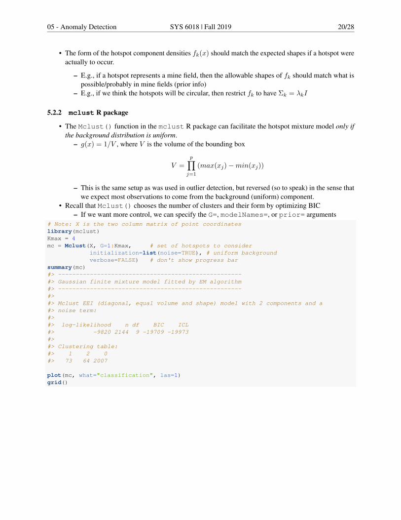
5.2.2 mclust R package

• The Mclust() function in the mclust R package can facilitate the hotspot mixture model only ifthe background distribution is uniform.

– g(x) = 1/V , where V is the volume of the bounding box

V =p∏j=1

(max(xj)−min(xj))

– This is the same setup as was used in outlier detection, but reversed (so to speak) in the sense thatwe expect most observations to come from the background (uniform) component.

• Recall that Mclust() chooses the number of clusters and their form by optimizing BIC– If we want more control, we can specify the G=, modelNames=, or prior= arguments

# Note: X is the two column matrix of point coordinateslibrary(mclust)Kmax = 4mc = Mclust(X, G=1:Kmax, # set of hotspots to consider

initialization=list(noise=TRUE), # uniform backgroundverbose=FALSE) # don't show progress bar

summary(mc)#> ----------------------------------------------------#> Gaussian finite mixture model fitted by EM algorithm#> ----------------------------------------------------#>#> Mclust EEI (diagonal, equal volume and shape) model with 2 components and a#> noise term:#>#> log-likelihood n df BIC ICL#> -9820 2144 9 -19709 -19973#>#> Clustering table:#> 1 2 0#> 73 64 2007

plot(mc, what="classification", las=1)grid()


0 2 4 6 8 10

0

2

4

6

8

10

x

y

5.3 Spatial Scan Statistic

The spatial scan statistic is an approach to detect spatial hotspots (sometimes called clusters) that adjusts formultiple testing.

5.3.1 Set-up

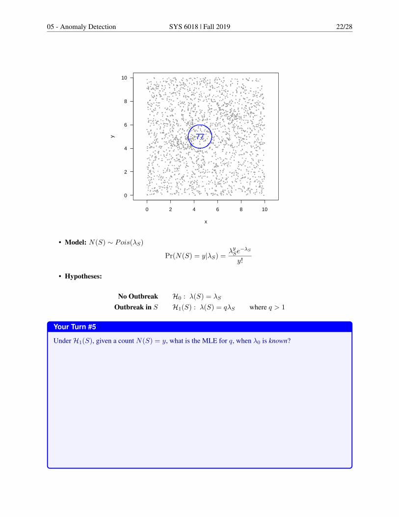
• Let S be a spatial region (e.g., circle)• Let N(S) be the number of events in S• Only focus on the region S; ignore everywhere else for now (but we eventually need to scan over all

regions)


0 2 4 6 8 10

0

2

4

6

8

10

x

y 77

• Model: N(S) ∼ Pois(λS)

Pr(N(S) = y|λS) = λySe−λS

y!

• Hypotheses:

No Outbreak H0 : λ(S) = λS

Outbreak in S H1(S) : λ(S) = qλS where q > 1

Your Turn #5

UnderH1(S), given a count N(S) = y, what is the MLE for q, when λ0 is known?


• Test Statistic: D(S)– Use Likelihood Ratio– Consider that λS is known

D(S): Likelihood Ratio Test Statistic

5.3.2 Significance Testing

• Simulate N0’s according toH0. N0 ∼ Pois(λS)• Calculate D0(S) for each simulation• Estimated p-value is the proportion of times that the simulated D0’s exceed y (observed)

• Example:– For the data in the plot, suppose λS = 63 for region S (blue circle)– We observed N(S) = 77– D(S) = (77

63)77 exp(63− 77) = 4.2701

Pr(D(S) ≥ 4.2701|H0, λ0 = 63) = Pr(N0(S) ≥ 77|λ0 = 63)= R: 1-ppois(77-1, lambda=63)

= 0.0479

– Significance! Are you ready to conclude that S is a hotspot?

That number is a p-value.

5.3.3 Multiple Testing

• Before we jump the gun, remember that we want to search the entire area for hotspots.

• If we considered a different region S′, but with same λ0 = 63, what is the probability that we wouldget D(S′) ≥ 4.2701, even if S′ is not a hotspot?

Your Turn #6

If we searched 5 non-overlapping regions S1, . . . , S5 (all with λ0 = 63), what is the probability that atleast one will have Dj(S) ≥ 4.2701, even if there are no hotspots?


• The probability of at least one false alarm starts to grow fast as the number of tests increases

• There are a few options:

1. Bonferroni: Only rejectH0 if p-value ≤ α/K, where K is the number of tests/comparisons– Can be too conservative if the tests are correlated

2. Scan Statistics (i.e., only test significance of the maximum score)

5.3.4 Spatial Search

• Let S be the search set, the set of spatial regions that will be searched– Every S will be in S (i.e., S ∈ S ∀S)

• The spatial regions may be restricted by size and/or shape. E.g.,– all balls/circles of radius r (or areas πr2)– All ellipses of area a

0 2 4 6 8 10

0

2

4

6

8

10

x

y 77

Ball of radius = 1

0 2 4 6 8 10

0

2

4

6

8

10

x

y

296

Ball of radius = 2

0 2 4 6 8 10

0

2

4

6

8

10

x

y

339

Ellipse of area = 15

• Scan the search windows over all locations and record the counts, N(S) and corresponding discrepancyscores D(S).

Click on image to see animation

●

●

●

●●

●

●

●

● ●

●

●

●

●

●●

●

●

●

●●

●

●

●

●

●

●

●

●

●

●

●

●

●

●

●

●

●

●

●

●

●

●

●

●

●

●

●●

●

●●

●●

●

●

●●

●

●

●

●

●

●

●

●

●

●

●●

●

●

●

●

●

●

●

●

●

●

●

●

●

●

●

●

●

●

●

●

●

●

●

●

●

●

●

●

●

●

●

●

●

●

●

●

●

●

●

●

●

●

●

●

●

●

●

●

●

●

●

●

●

●

●

●

●

●

●

●

●

●

●

●

●

●

●

●

●

●

●

●

●

●

●●

●

●

●

●

●

●

●

●

●

●

●

●

●

●

●

●

●

●

●

●

●

●

●

●

●

●

●

●

●

●

●

●

●

●

●

●

●

●

●

●

●

●

●

●

●

●

●

●

●

●

●

●

●

●

●

●

●

●

●

●

●

●

●

●

●

●

●

●

●

●●

●

●

●

●

●

●

●

●

●

●

●

●

●

●

●

●

●

●

●

●

●

●

●

●

●

●

●

●

●

●

●

●

●

●

●

●

●

●

●

●

●

●

●

●

●

●

●

●

●

●

●

●

●

●

●

●

●

●

●

●

●

●

●

●

●●

●

●

●

●

●

●

●

●

●

●

●

●

●

●

●

●

●

●

●

●

●

●

●

●

●

●

●

●

●

●

●

●

●

●

●

●

●

●

●

●

●

●

●

●

●

●

●

●

●

●

●

●

●

●

●

●

●

●

●

●

●

●

●

●

●

●

●

●

●

●

●

●

●

●

●

●

●

●

●

●

●

●

●

●

●

●●

●

●

●

●

●

●

●

●

●

●

●

●

●

●

●

●

●

●

●

●

●

●

●

●

●

●

●

●

●

●

●

●

●

●

●

●

●

●

●

●

●

●

●

●

●

●

●

●

●

●

●

●

●

●

●

●

●

●

●

●

●

●

●

●

●

●

●

●

●

●

●

●

●

●

●

●

●

●

●

●

●

●

●

●

●

●

●

●

●

●

●

●

●

●

●

●

●

●

●

●

●

●

●

●

●

●

●

●

●

●

●

●

●

●

●

●

●

●

●

●

●

●

●

●

●

●

●

●

●

●

●

●

●

●

●

●

●

●

●●

●

●

●

●

●

●

●

●

●

●

●

●

●

●

●

●

●

●

●

●

●

●

●

●

●

●

●

●

●

●

●

●

●

●

●

●

●

●

●

●

●

●

●

●

●

●

●

●

●

●

●

●

●

●

●

●

●

●

●

●

●

●

●

●

●

●

●

●

●

●

●

●

●

●

●

●

●

●

●

●

●

●

●

●

●

●

●

●

●

●

●

●

●

●

●

●

●

●

●

●

●

●

●

●

●

●

●

●

●

●●

●

●

●

●

●

●

●

●

●

●

●

●

●

●

●

●

●

●

●

●

●

●

●

●

●

●

●

●

●

●

●

●

●

●

●

●

●

●

●

●

●

●●

●

●

●

●

●

●

●

●

●

●

●

●

●

●

●

●

●

●

●

●

●

●

●

●

●

●

●

●

●

●

●

●

●

●

●

●

●

●

●

●

●

●

●

●

●

●

●

●

●

●

●

●

●

●

●

●

●

●

●

●

●

●

●

●

●

●

●●

●

●

●

●

●

●

●

●

●

●

●

●

●

●

●

●

●

●

●

●

●

●

●

●

●

●

●

●

●

●

●

●

●

●

●

●

●

●

●

●

●

●

●

●

●

●

●

●

●

●

●

●

●

●

●

●

●

●

●

●

●

●

●

●

●

●

●

●

●●

●

●

●

●

●

●

●

●

●

●

●

●

●

●

●

●

●

●

●

●

●

●

●

●

●

●

●

●

●

●

●

●

●

●

●

●

●

●

●

●

●

●

●

●

●

●●

●

●

●

●

●

●

●

●

●

●

●

●

●

●

●

●

●

●

●

●●

●

●

●

●

●

●

●

●

●

●

●

●

●

●

●

●

●

●

●

●

●

●

●

●

●

●

●●

●

●

●

●

●

●

●

●

●

●

●

●

●

●

●

●

●

●

●

●

●

●

●

●

●

●

●

●

●

●

●

●

●

●

●

●

●

●

●

●

●

●

●

●

●

●

●

●

●

●

●

●

●

●

●

●

●

●

●

●

●

●

●●

●

●

●

●

●

●

●

●

●

●

●

●

●

●

●

●

●

●

●

●

●

●

●

●

●

●

●

●

●

●

●

●

●

●

●

●

●

●

●

●

●

●

●

●

●

●

●

●

● ●

●

●

●

●

●

●

●

●

●

●

●

●

●

●

●

●

●

●

●

●

●

●

●

●

●

●

●

●

●

●

●

●

●

●

●

●

●

●

●

●

●

●

●

●

●

●

●

●

●

●

●

●

●

●

●

●

●

●

●

●

●

●

●

●

●

●

●

●

●●

●

●●

●

●

●

●

●

●

●

●

●

●

●

●

●

●

●

●

●

●

●

●

●●

●

●

●

●

●

●

●

●

●

●

●

●

●

●

●

●

●

●

●

●

●

●

●

●

●

●

●

●

●

●

●

●

●

● ●

●

●

●

●

●

●

●

●

●

●

●

●

●

●

●

●

●

●

●

●

●

●

●

●

●

●

●

●

●

●

●

●

●

●

●

●

●

●

●

●

●

●

●

●

●

●

●

●

●

●

●

●

●

●

●

●

●●

●

●

●

●

●

●

●

●

●

●

●

●

●

●

●

●

●

●

●

●

●

●

●

●

●

●

●

●

●

●

●

●

●

●

●

●

●

●

●

●

●

●

●

●

●

●

●

●

●

●

●

●

●

●

●

●

●

●

●

●

●

●

●

●

●

●

●

●

●

●

●

●

●

●

●●

●

●

●

●

●●

●

●

●

●

●

●

●

●

●

●

●

●

●

●

●

●

●

●

●

●

●

●

●

●

●

●

●

●

●

●

●

●

●

●

●

●

●

●

●

●

●

●

●

●

●

●

●

●

●

●

●

●

●

●

●

●

●

●

●

●

●

●

●

●

●

●

●

●

●

●

●

●

●

●

●

●

●

●

●

●

●

●

●

●

●

●

●

●

●

●

●

●

●

●

●

●

●

●

●

●

●

●

●

●

●

●

●

●

●

●

●

●

●

●●

●

●

●

●

●

●

●

●

●

●

●●

●

●

●

●

●

●

●

●

●

●

●

●

●

●

●

●

●●

●

●

●

●

●

●

●

●

●

●

●

●

●

●

●

●

●

●

●

●

●

●

●

●

●

●

●

●

●

●

●

●

●

●

●

●

●

●

●

●

●

●

●

●

●

●

●

●

●

●

●

●

●

●

●

●

●

●

●

●

●

●

●

●

●

●

●

●

●

●

●

●

●

●

●

●

●

●

●

●

●

●

●

●

●

●

●

●

●

●

●

●

●

●

●

●

●

●

●

●

●

●

●

●

●

●

●

●

●

●

●

●

●

●

●

●

●

●

●

●

●

●

●

●

●

● ●

●

●

●

●

●

●

●

●

●

●

●

●

●●

●

●

●

●

●●

● ●

●

●

●

●

●

●

●

●

●

●

●

●

●

●

●

●

●

●

●

●

●

●

●

●

●

●

●

●

●

●

●

●

●

●

●

●

●

●

●

●

●

●

●

●

●

●

●

●

●

●

●

●

●

●

●

●

●

●

●

●

●

●

●

●

●

●

●

●

●

●

●

●

●

●

●

●

●

●

●

●

●

●

●

●

●

●

●

●

●●

●

●

●

●

●

●

●

●

●

●

●

●

●●

●

● ●

●

●

●

●

●

●

●

●

●

●

●

●

●

●

●

●

●

●

●

●

●

●

●

●

●

●

●

●

●

●

●

●

●

●

●

●

●

●

●

●

●

●

●

●

●

●

●

●

●

●

●

●

●

●

●

●

●

●

●

●

●

●

●

●

●

●

●

●

●

●

●

●

●

●

●

●

●

●

●

●

●

●

●

●

●

●

●

●

●

●

●

●

●

●

●

●

●

●

●

●

●

●

●

●

●

●

●

●

●

●

●

●

●

●

●

●

●

●

●

●

●

●

●

●

●

●

●

●

●

●

●

●

●

●

●

●

●

●

●

●

●

●

●

●

●

●

●

●

●

●

●

●

●

●

●

●

●

●

●

●

●

●

●

●

●

●

●

●

●

●

●

●

● ●

●

●

●

●

●

●

●

●

●

●

●

●

●

●

●

●

●

●

●

●

●

●

●

●

●

●

●

●

●

●

●

●

●

●

●

●

●

●

●

●

●

●

●

●

●

●

●

●

●

●

●

●

●

●

●

●

●

●

●

●

●

●

●

●

●

●

●

●

●●

●

●

●

●

●

●

●

●

●

●

●

●

●

●

●

●

●

●

●

●

●

●

●

●

●

●

●

●

●

●

●

●

●

●

●

●

●

●

●

●

●

●

●

●●

●

●

●

●

●

●

●

●

●

●

●

●

●

●

●

●

●

●

●

●

●

●

●

●

●

●

●

●

●

●

●

●

●

●

●

●

●

●

●

●

●

●

●

●

●

●

●

●

●

●

●

●

●

●

●

●

●

●

●

●

●

●

●

●

●

●

● ●

●

●

●

●

●

●

●

●

●

●

●

●

●

●

●

●

●

●

●

●

●

●

●

●

●

●

●

●

●

●

●

●

●

●

●

●

●

●

●

●

●

●

●

●

●

●

●

●

●

●

●

●

●

●

●

●

●

●

●

●

●

●

●

●

●

●

●

●

●

●

●

●

●

●

●

●

●

●

●

●

114

0.0

2.5

5.0

7.5

10.0

0.0 2.5 5.0 7.5 10.0

x

y

30

60

90

n

counts in window with radius = 1

●

●

●

●●

●

●

●

● ●

●

●

●

●

●●

●

●

●

●●

●

●

●

●

●

●

●

●

●

●

●

●

●

●

●

●

●

●

●

●

●

●

●

●

●

●

●●

●

●●

●●

●

●

●●

●

●

●

●

●

●

●

●

●

●

●●

●

●

●

●

●

●

●

●

●

●

●

●

●

●

●

●

●

●

●

●

●

●

●

●

●

●

●

●

●

●

●

●

●

●

●

●

●

●

●

●

●

●

●

●

●

●

●

●

●

●

●

●

●

●

●

●

●

●

●

●

●

●

●

●

●

●

●

●

●

●

●

●

●

●

●●

●

●

●

●

●

●

●

●

●

●

●

●

●

●

●

●

●

●

●

●

●

●

●

●

●

●

●

●

●

●

●

●

●

●

●

●

●

●

●

●

●

●

●

●

●

●

●

●

●

●

●

●

●

●

●

●

●

●

●

●

●

●

●

●

●

●

●

●

●

●●

●

●

●

●

●

●

●

●

●

●

●

●

●

●

●

●

●

●

●

●

●

●

●

●

●

●

●

●

●

●

●

●

●

●

●

●

●

●

●

●

●

●

●

●

●

●

●

●

●

●

●

●

●

●

●

●

●

●

●

●

●

●

●

●

●●

●

●

●

●

●

●

●

●

●

●

●

●

●

●

●

●

●

●

●

●

●

●

●

●

●

●

●

●

●

●

●

●

●

●

●

●

●

●

●

●

●

●

●

●

●

●

●

●

●

●

●

●

●

●

●

●

●

●

●

●

●

●

●

●

●

●

●

●

●

●

●

●

●

●

●

●

●

●

●

●

●

●

●

●

●

●●

●

●

●

●

●

●

●

●

●

●

●

●

●

●

●

●

●

●

●

●

●

●

●

●

●

●

●

●

●

●

●

●

●

●

●

●

●

●

●

●

●

●

●

●

●

●

●

●

●

●

●

●

●

●

●

●

●

●

●

●

●

●

●

●

●

●

●

●

●

●

●

●

●

●

●

●

●

●

●

●

●

●

●

●

●

●

●

●

●

●

●

●

●

●

●

●

●

●

●

●

●

●

●

●

●

●

●

●

●

●

●

●

●

●

●

●

●

●

●

●

●

●

●

●

●

●

●

●

●

●

●

●

●

●

●

●

●

●

●●

●

●

●

●

●

●

●

●

●

●

●

●

●

●

●

●

●

●

●

●

●

●

●

●

●

●

●

●

●

●

●

●

●

●

●

●

●

●

●

●

●

●

●

●

●

●

●

●

●

●

●

●

●

●

●

●

●

●

●

●

●

●

●

●

●

●

●

●

●

●

●

●

●

●

●

●

●

●

●

●

●

●

●

●

●

●

●

●

●

●

●

●

●

●

●

●

●

●

●

●

●

●

●

●

●

●

●

●

●

●●

●

●

●

●

●

●

●

●

●

●

●

●

●

●

●

●

●

●

●

●

●

●

●

●

●

●

●

●

●

●

●

●

●

●

●

●

●

●

●

●

●

●●

●

●

●

●

●

●

●

●

●

●

●

●

●

●

●

●

●

●

●

●

●

●

●

●

●

●

●

●

●

●

●

●

●

●

●

●

●

●

●

●

●

●

●

●

●

●

●

●

●

●

●

●

●

●

●

●

●

●

●

●

●

●

●

●

●

●

●●

●

●

●

●

●

●

●

●

●

●

●

●

●

●

●

●

●

●

●

●

●

●

●

●

●

●

●

●

●

●

●

●

●

●

●

●

●

●

●

●

●

●

●

●

●

●

●

●

●

●

●

●

●

●

●

●

●

●

●

●

●

●

●

●

●

●

●

●

●●

●

●

●

●

●

●

●

●

●

●

●

●

●

●

●

●

●

●

●

●

●

●

●

●

●

●

●

●

●

●

●

●

●

●

●

●

●

●

●

●

●

●

●

●

●

●●

●

●

●

●

●

●

●

●

●

●

●

●

●

●

●

●

●

●

●

●●

●

●

●

●

●

●

●

●

●

●

●

●

●

●

●

●

●

●

●

●

●

●

●

●

●

●

●●

●

●

●

●

●

●

●

●

●

●

●

●

●

●

●

●

●

●

●

●

●

●

●

●

●

●

●

●

●

●

●

●

●

●

●

●

●

●

●

●

●

●

●

●

●

●

●

●

●

●

●

●

●

●

●

●

●

●

●

●

●

●

●●

●

●

●

●

●

●

●

●

●

●

●

●

●

●

●

●

●

●

●

●

●

●

●

●

●

●

●

●

●

●

●

●

●

●

●

●

●

●

●

●

●

●

●

●

●

●

●

●

● ●

●

●

●

●

●

●

●

●

●

●

●

●

●

●

●

●

●

●

●

●

●

●

●

●

●

●

●

●

●

●

●

●

●

●

●

●

●

●

●

●

●

●

●

●

●

●

●

●

●

●

●

●

●

●

●

●

●

●

●

●

●

●

●

●

●

●

●

●

●●

●

●●

●

●

●

●

●

●

●

●

●

●

●

●

●

●

●

●

●

●

●

●

●●

●

●

●

●

●

●

●

●

●

●

●

●

●

●

●

●

●

●

●

●

●

●

●

●

●

●

●

●

●

●

●

●

●

● ●

●

●

●

●

●

●

●

●

●

●

●

●

●

●

●

●

●

●

●

●

●

●

●

●

●

●

●

●

●

●

●

●

●

●

●

●

●

●

●

●

●

●

●

●

●

●

●

●

●

●

●

●

●

●

●

●

●●

●

●

●

●

●

●

●

●

●

●

●

●

●

●

●

●

●

●

●

●

●

●

●

●

●

●

●

●

●

●

●

●

●

●

●

●

●

●

●

●

●

●

●

●

●

●

●

●

●

●

●

●

●

●

●

●

●

●

●

●

●

●

●

●

●

●

●

●

●

●

●

●

●

●

●●

●

●

●

●

●●

●

●

●

●

●

●

●

●

●

●

●

●

●

●

●

●

●

●

●

●

●

●

●

●

●

●

●

●

●

●

●

●

●

●

●

●

●

●

●

●

●

●

●

●

●

●

●

●

●

●

●

●

●

●

●

●

●

●

●

●

●

●

●

●

●

●

●

●

●

●

●

●

●

●

●

●

●

●

●

●

●

●

●

●

●

●

●

●

●

●

●

●

●

●

●

●

●

●

●

●

●

●

●

●

●

●

●

●

●

●

●

●

●

●●

●

●

●

●

●

●

●

●

●

●

●●

●

●

●

●

●

●

●

●

●

●

●

●

●

●

●

●

●●

●

●

●

●

●

●

●

●

●

●

●

●

●

●

●

●

●

●

●

●

●

●

●

●

●

●

●

●

●

●

●

●

●

●

●

●

●

●

●

●

●

●

●

●

●

●

●

●

●

●

●

●

●

●

●

●

●

●

●

●

●

●

●

●

●

●

●

●

●

●

●

●

●

●

●

●

●

●

●

●

●

●

●

●

●

●

●

●

●

●

●

●

●

●

●

●

●

●

●

●

●

●

●

●

●

●

●

●

●

●

●

●

●

●

●

●

●

●

●

●

●

●

●

●

●

● ●

●

●

●

●

●

●

●

●

●

●

●

●

●●

●

●

●

●

●●

● ●

●

●

●

●

●

●

●

●

●

●

●

●

●

●

●

●

●

●

●

●

●

●

●

●

●

●

●

●

●

●

●

●

●

●

●

●

●

●

●

●

●

●

●

●

●

●

●

●

●

●

●

●

●

●

●

●

●

●

●

●

●

●

●

●

●

●

●

●

●

●

●

●

●

●

●

●

●

●

●

●

●

●

●

●

●

●

●

●

●●

●

●

●

●

●

●

●

●

●

●

●

●

●●

●

● ●

●

●

●

●

●

●

●

●

●

●

●

●

●

●

●

●

●

●

●

●

●

●

●

●

●

●

●

●

●

●

●

●

●

●

●

●

●

●

●

●

●

●

●

●

●

●

●

●

●

●

●

●

●

●

●

●

●

●

●

●

●

●

●

●

●

●

●

●

●

●

●

●

●

●

●

●

●

●

●

●

●

●

●

●

●

●

●

●

●

●

●

●

●

●

●

●

●

●

●

●

●

●

●

●

●

●

●

●

●

●

●

●

●

●

●

●

●

●

●

●

●

●

●

●

●

●

●

●

●

●

●

●

●

●

●

●

●

●

●

●

●

●

●

●

●

●

●

●

●

●

●

●

●

●

●

●

●

●

●

●

●

●

●

●

●

●

●

●

●

●

●

●

● ●

●

●

●

●

●

●

●

●

●

●

●

●

●

●

●

●

●

●

●

●

●

●

●

●

●

●

●

●

●

●

●

●

●

●

●

●

●

●

●

●

●

●

●

●

●

●

●

●

●

●

●

●

●

●

●

●

●

●

●

●

●

●

●

●

●

●

●

●

●●

●

●

●

●

●

●

●

●

●

●

●

●

●

●

●

●

●

●

●

●

●

●

●

●

●

●

●

●

●

●

●

●

●

●

●

●

●

●

●

●

●

●

●

●●

●

●

●

●

●

●

●

●

●

●

●

●

●

●

●

●

●

●

●

●

●

●

●

●

●

●

●

●

●

●

●

●

●

●

●

●

●

●

●

●

●

●

●

●

●

●

●

●

●

●

●

●

●

●

●

●

●

●

●

●

●

●

●

●

●

●

● ●

●

●

●

●

●

●

●

●

●

●

●

●

●

●

●

●

●

●

●

●

●

●

●

●

●

●

●

●

●

●

●

●

●

●

●

●

●

●

●

●

●

●

●

●

●

●

●

●

●

●

●

●

●

●

●

●

●

●

●

●

●

●

●

●

●

●

●

●

●

●

●

●

●

●

●

●

●

●

●

●

16.6

0.0

2.5

5.0

7.5

10.0

0.0 2.5 5.0 7.5 10.0

x

y

0

4

8

12

16

D

log LR in window with radius = 1

https://github.com/mdporter/SYS6018/blob/master/other/satscan_demo1.gif

https://github.com/mdporter/SYS6018/blob/master/other/satscan_demo2.gif


5.3.5 Scan Stat (Test Statistic)

• The spatial scan stat test statistic, for balls of radius r, is the discrepancy score (log LR) for the regionthat gives the maximum discrepancy

D∗r = maxS∈Sr

Dr(S)

– So, move the balls over the entire area, calculate the log LR for each ball, and use the largestvalue as the test statistic

5.3.6 Results

0.0

2.5

5.0

7.5

10.0

0.0 2.5 5.0 7.5 10.0x

y

25

50

75

100

125

n


0.0

2.5

5.0

7.5

10.0

0.0 2.5 5.0 7.5 10.0x

y100

200

300

n


0.0

2.5

5.0

7.5

10.0

0.0 2.5 5.0 7.5 10.0x

y

0

10

20

D


0.0

2.5

5.0

7.5

10.0

0.0 2.5 5.0 7.5 10.0x

y

0

100

200

300

D


• NOTE: There is strong connection to kernel density estimation! Do you see how we can build the searchfrom special KDE functions?

• Maximum Scores (aka the scan statistics)

radius x y n D*

1 3.13 4.75 131 27.92 3.13 5.96 363 335.7

5.3.7 Monte Carlo Significance Testing

• Is one of the D∗’s large enough to conclude there is a hotspot?


• What radius should be used?

• To answer these questions, we need to find the distribution of D∗ under the null hypothesis of nohotspots

1. Simulate from the null hypothesis

• We assume the data came from a spatial Poisson point process with known intensity λ(x)• Simulate n events (n is the number of events we observed)• Density is f(x) = λ0(x)/

∫λ0(u) du

2. Search for Hotspots

• Must choose the shapes/sizes for the potential hotspots

3. Record scan statistics

4. Redo steps 1-2 M times

5. Calculate p-values

• p-value = 1+∑

m1(D∗

m≥D∗obs)

1+M

radius=1 radius=2

85 90 95 100 105 300 320 340

0

10

20

30

40

0

10

20

30

40

n

coun

t

count

radius=1 radius=2

5.0 7.5 10.0 225 250 275 300

0

10

20

30

40

0

10

20

30

40

D

coun

t

log LR

• No simulation exceeded our observed scores (D∗r=1 = 27.90 and D∗r=2 = 335.71).– Thus, very small estimated p-values (i.e., 1/(M + 1))


– Thus, there is likely at least one hotspot (i.e., at least one circle of radius 1 and radius 2 that hasan unusually large count)

0 2 4 6 8 10

0

2

4

6

8

10

x

y

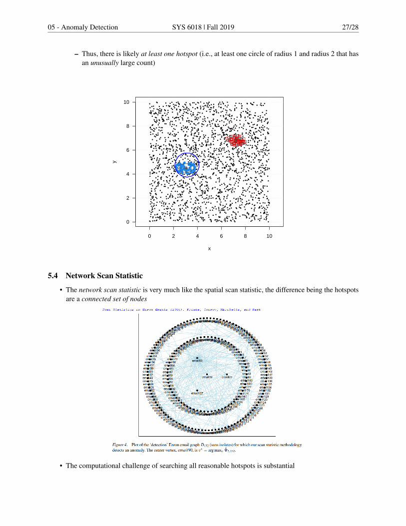
5.4 Network Scan Statistic

• The network scan statistic is very much like the spatial scan statistic, the difference being the hotspotsare a connected set of nodes

• The computational challenge of searching all reasonable hotspots is substantial


6 Outbreak Detection

• Consider having the spatial observations occurring over time.

– E.g., daily, weekly, hourly

• Denote N(t, S) as the number of events in spatial region S at time period t

• There is a time point τ when an outbreak starts

H0 : λ(t, S) = λ0(t) for all t

H1(τ, S) : λ(t, S) ={λ0(t) for t < τ

q(t)λ0(t) for t ≥ τ and q(t) > 1

time = 1 time = 2 time = 3

time = 4 time = 5 time = 6

• One option is to compute D∗(t) over each time t and look for the time when there is an increase– Use Statistical Process Control (SPC, control charts)

• If the signal (i.e., outbreak) is small, it may take many time periods before there is enough evidence todetect the outbreak

– Another option is to include time into the likelihood ratio test statistic– See: Kulldorff, M. (2001), Prospective time periodic geographical disease surveillance using a

scan statistic. Journal of the Royal Statistical Society: Series A (Statistics in Society), 164: 61-72for more details

https://rss.onlinelibrary.wiley.com/action/showCitFormats?doi=10.1111%2F1467-985X.00186

https://rss.onlinelibrary.wiley.com/action/showCitFormats?doi=10.1111%2F1467-985X.00186

05 - Anomaly Detection - GitHub Pages · 05 - Anomaly Detection SYS 6018 | Fall 2019 3/28 1.3...

Documents

Transcript of 05 - Anomaly Detection - GitHub Pages · 05 - Anomaly Detection SYS 6018 | Fall 2019 3/28 1.3...