042-2009: Manipulating OLAP Cubes: Advanced Techniques...

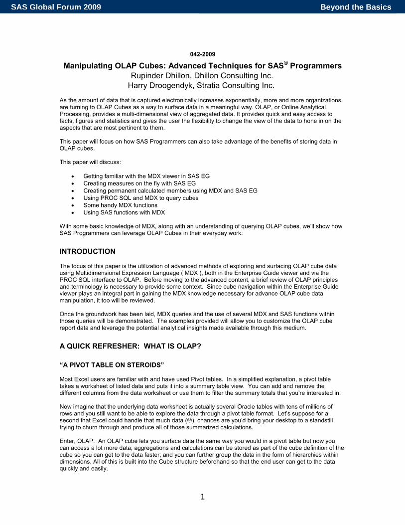
1

042-2009

Manipulating OLAP Cubes: Advanced Techniques for SAS® Programmers

Rupinder Dhillon, Dhillon Consulting Inc.

Harry Droogendyk, Stratia Consulting Inc. As the amount of data that is captured electronically increases exponentially, more and more organizations are turning to OLAP Cubes as a way to surface data in a meaningful way. OLAP, or Online Analytical Processing, provides a multi-dimensional view of aggregated data. It provides quick and easy access to facts, figures and statistics and gives the user the flexibility to change the view of the data to hone in on the aspects that are most pertinent to them. This paper will focus on how SAS Programmers can also take advantage of the benefits of storing data in OLAP cubes. This paper will discuss:

• Getting familiar with the MDX viewer in SAS EG

• Creating measures on the fly with SAS EG

• Creating permanent calculated members using MDX and SAS EG

• Using PROC SQL and MDX to query cubes

• Some handy MDX functions

• Using SAS functions with MDX With some basic knowledge of MDX, along with an understanding of querying OLAP cubes, we’ll show how SAS Programmers can leverage OLAP Cubes in their everyday work.

INTRODUCTION The focus of this paper is the utilization of advanced methods of exploring and surfacing OLAP cube data using Multidimensional Expression Language ( MDX ), both in the Enterprise Guide viewer and via the PROC SQL interface to OLAP. Before moving to the advanced content, a brief review of OLAP principles and terminology is necessary to provide some context. Since cube navigation within the Enterprise Guide viewer plays an integral part in gaining the MDX knowledge necessary for advance OLAP cube data manipulation, it too will be reviewed. Once the groundwork has been laid, MDX queries and the use of several MDX and SAS functions within those queries will be demonstrated. The examples provided will allow you to customize the OLAP cube report data and leverage the potential analytical insights made available through this medium.

A QUICK REFRESHER: WHAT IS OLAP?

“A PIVOT TABLE ON STEROIDS” Most Excel users are familiar with and have used Pivot tables. In a simplified explanation, a pivot table takes a worksheet of listed data and puts it into a summary table view. You can add and remove the different columns from the data worksheet or use them to filter the summary totals that you’re interested in. Now imagine that the underlying data worksheet is actually several Oracle tables with tens of millions of rows and you still want to be able to explore the data through a pivot table format. Let’s suppose for a second that Excel could handle that much data (�), chances are you’d bring your desktop to a standstill trying to churn through and produce all of those summarized calculations. Enter, OLAP. An OLAP cube lets you surface data the same way you would in a pivot table but now you can access a lot more data; aggregations and calculations can be stored as part of the cube definition of the cube so you can get to the data faster; and you can further group the data in the form of hierarchies within dimensions. All of this is built into the Cube structure beforehand so that the end user can get to the data quickly and easily.

Beyond the BasicsSAS Global Forum 2009

2

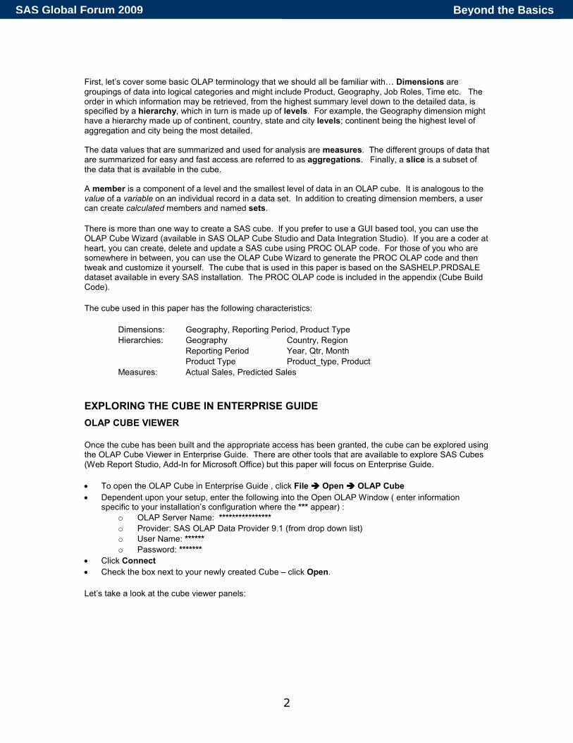
First, let’s cover some basic OLAP terminology that we should all be familiar with… Dimensions are groupings of data into logical categories and might include Product, Geography, Job Roles, Time etc. The order in which information may be retrieved, from the highest summary level down to the detailed data, is specified by a hierarchy, which in turn is made up of levels. For example, the Geography dimension might have a hierarchy made up of continent, country, state and city levels; continent being the highest level of aggregation and city being the most detailed. The data values that are summarized and used for analysis are measures. The different groups of data that are summarized for easy and fast access are referred to as aggregations. Finally, a slice is a subset of the data that is available in the cube. A member is a component of a level and the smallest level of data in an OLAP cube. It is analogous to the value of a variable on an individual record in a data set. In addition to creating dimension members, a user can create calculated members and named sets.

There is more than one way to create a SAS cube. If you prefer to use a GUI based tool, you can use the OLAP Cube Wizard (available in SAS OLAP Cube Studio and Data Integration Studio). If you are a coder at heart, you can create, delete and update a SAS cube using PROC OLAP code. For those of you who are somewhere in between, you can use the OLAP Cube Wizard to generate the PROC OLAP code and then tweak and customize it yourself. The cube that is used in this paper is based on the SASHELP.PRDSALE dataset available in every SAS installation. The PROC OLAP code is included in the appendix (Cube Build Code).

The cube used in this paper has the following characteristics:

Dimensions: Geography, Reporting Period, Product Type

Hierarchies: Geography Country, Region

Reporting Period Year, Qtr, Month

Product Type Product_type, Product

Measures: Actual Sales, Predicted Sales

EXPLORING THE CUBE IN ENTERPRISE GUIDE

OLAP CUBE VIEWER

Once the cube has been built and the appropriate access has been granted, the cube can be explored using the OLAP Cube Viewer in Enterprise Guide. There are other tools that are available to explore SAS Cubes (Web Report Studio, Add-In for Microsoft Office) but this paper will focus on Enterprise Guide.

• To open the OLAP Cube in Enterprise Guide , click File �� Open �� OLAP Cube

• Dependent upon your setup, enter the following into the Open OLAP Window ( enter information specific to your installation’s configuration where the *** appear) :

o OLAP Server Name: ****************

o Provider: SAS OLAP Data Provider 9.1 (from drop down list)

o User Name: ******

o Password: *******

• Click Connect

• Check the box next to your newly created Cube – click Open.

Let’s take a look at the cube viewer panels:


3

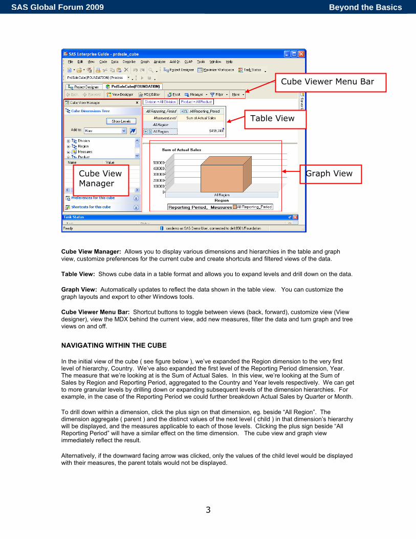
Cube View Manager: Allows you to display various dimensions and hierarchies in the table and graph view, customize preferences for the current cube and create shortcuts and filtered views of the data.

Table View: Shows cube data in a table format and allows you to expand levels and drill down on the data.

Graph View: Automatically updates to reflect the data shown in the table view. You can customize the

graph layouts and export to other Windows tools.

Cube Viewer Menu Bar: Shortcut buttons to toggle between views (back, forward), customize view (View designer), view the MDX behind the current view, add new measures, filter the data and turn graph and tree views on and off.

NAVIGATING WITHIN THE CUBE

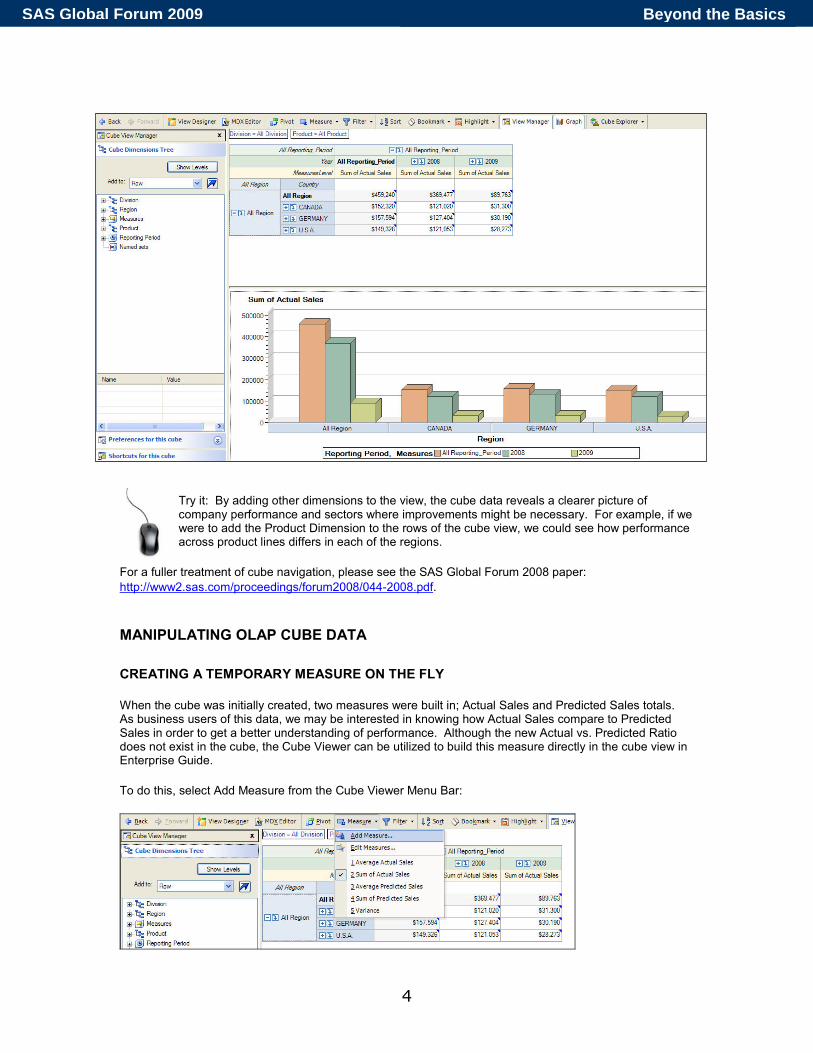
In the initial view of the cube ( see figure below ), we’ve expanded the Region dimension to the very first level of hierarchy, Country. We’ve also expanded the first level of the Reporting Period dimension, Year. The measure that we’re looking at is the Sum of Actual Sales. In this view, we’re looking at the Sum of Sales by Region and Reporting Period, aggregated to the Country and Year levels respectively. We can get to more granular levels by drilling down or expanding subsequent levels of the dimension hierarchies. For example, in the case of the Reporting Period we could further breakdown Actual Sales by Quarter or Month.

To drill down within a dimension, click the plus sign on that dimension, eg. beside “All Region”. The dimension aggregate ( parent ) and the distinct values of the next level ( child ) in that dimension’s hierarchy will be displayed, and the measures applicable to each of those levels. Clicking the plus sign beside “All Reporting Period” will have a similar effect on the time dimension. The cube view and graph view immediately reflect the result.

Alternatively, if the downward facing arrow was clicked, only the values of the child level would be displayed with their measures, the parent totals would not be displayed.

Cube Viewer Menu Bar

Table View

Graph View Cube View

Manager


4

Try it: By adding other dimensions to the view, the cube data reveals a clearer picture of company performance and sectors where improvements might be necessary. For example, if we were to add the Product Dimension to the rows of the cube view, we could see how performance across product lines differs in each of the regions.

For a fuller treatment of cube navigation, please see the SAS Global Forum 2008 paper:

http://www2.sas.com/proceedings/forum2008/044-2008.pdf.

MANIPULATING OLAP CUBE DATA

CREATING A TEMPORARY MEASURE ON THE FLY

When the cube was initially created, two measures were built in; Actual Sales and Predicted Sales totals. As business users of this data, we may be interested in knowing how Actual Sales compare to Predicted Sales in order to get a better understanding of performance. Although the new Actual vs. Predicted Ratio does not exist in the cube, the Cube Viewer can be utilized to build this measure directly in the cube view in Enterprise Guide.

To do this, select Add Measure from the Cube Viewer Menu Bar:


5

This will launch a wizard that will guide you through the rest of the steps needed to create this measure.

Step 1: Name the measure Step 2: Specify the type of measure you’re

creating. In this case we’re doing a simple calculation

Step 3: Build the calculation by selecting ‘Ratio’ Step 4: Add the Percent format. as the Calculation and the Sum of Actual Sales and the Sum of Predicted Sales as the formula elements.


6

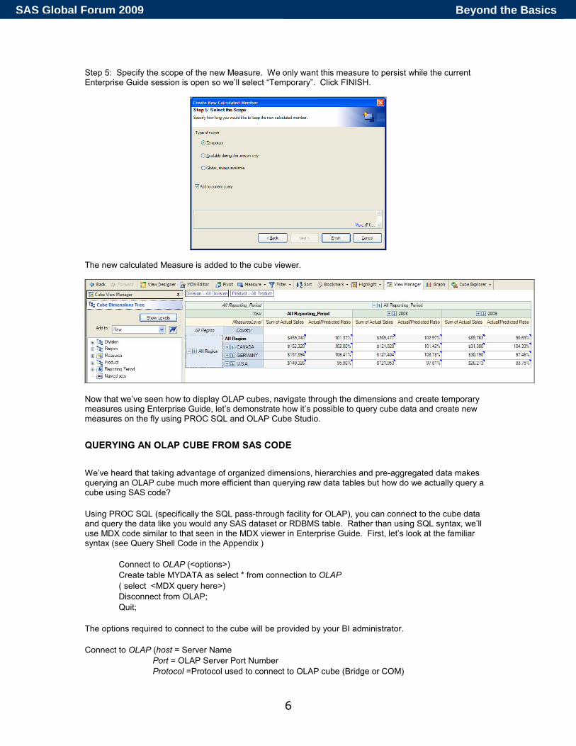
Step 5: Specify the scope of the new Measure. We only want this measure to persist while the current Enterprise Guide session is open so we’ll select “Temporary”. Click FINISH.

The new calculated Measure is added to the cube viewer.

Now that we’ve seen how to display OLAP cubes, navigate through the dimensions and create temporary measures using Enterprise Guide, let’s demonstrate how it’s possible to query cube data and create new measures on the fly using PROC SQL and OLAP Cube Studio.

QUERYING AN OLAP CUBE FROM SAS CODE

We’ve heard that taking advantage of organized dimensions, hierarchies and pre-aggregated data makes querying an OLAP cube much more efficient than querying raw data tables but how do we actually query a cube using SAS code?

Using PROC SQL (specifically the SQL pass-through facility for OLAP), you can connect to the cube data and query the data like you would any SAS dataset or RDBMS table. Rather than using SQL syntax, we’ll use MDX code similar to that seen in the MDX viewer in Enterprise Guide. First, let’s look at the familiar syntax (see Query Shell Code in the Appendix )

Connect to OLAP (<options>)

Create table MYDATA as select * from connection to OLAP

( select <MDX query here>)

Disconnect from OLAP;

Quit;

The options required to connect to the cube will be provided by your BI administrator.

Connect to OLAP (host = Server Name

Port = OLAP Server Port Number

Protocol =Protocol used to connect to OLAP cube (Bridge or COM)


7

User = User ID

Pass = User Password

Repository =Metadata Repository

OLAP_schema =The schema in which the cube is defined);

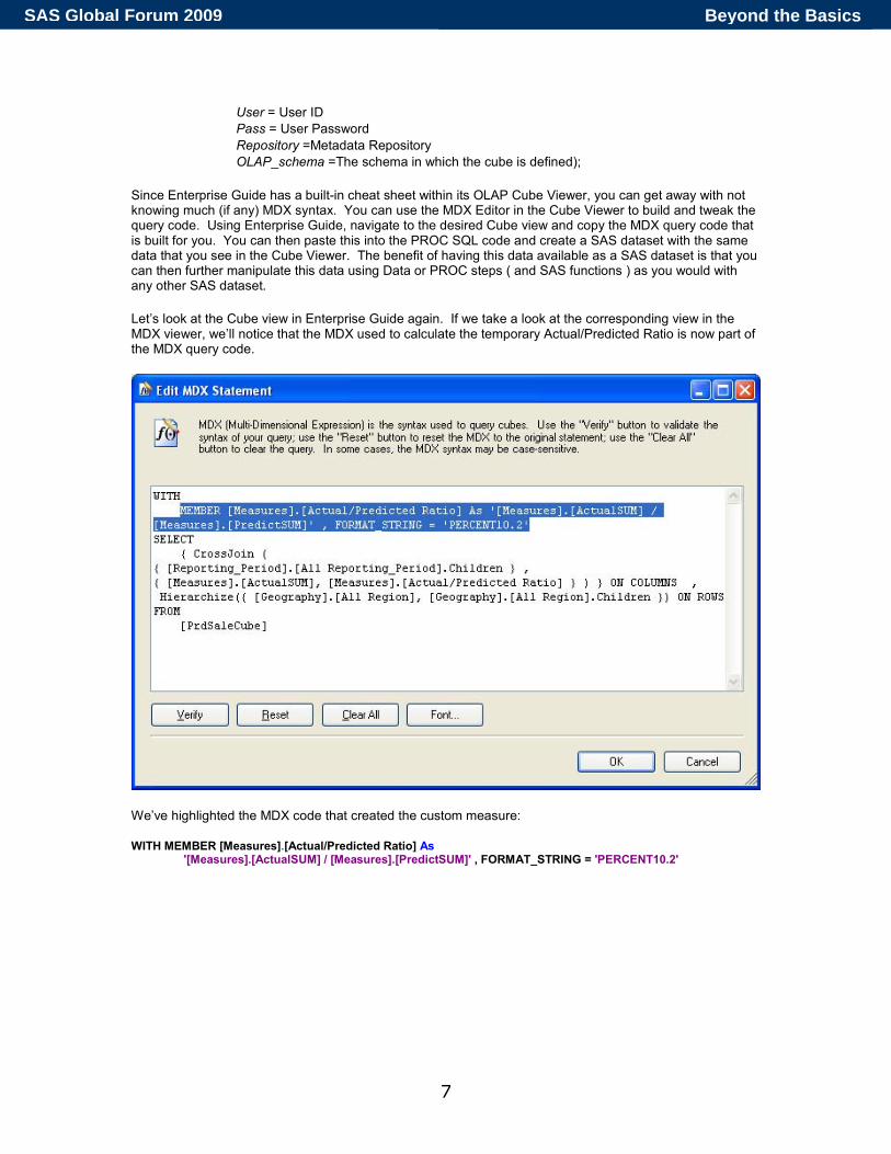
Since Enterprise Guide has a built-in cheat sheet within its OLAP Cube Viewer, you can get away with not knowing much (if any) MDX syntax. You can use the MDX Editor in the Cube Viewer to build and tweak the query code. Using Enterprise Guide, navigate to the desired Cube view and copy the MDX query code that is built for you. You can then paste this into the PROC SQL code and create a SAS dataset with the same data that you see in the Cube Viewer. The benefit of having this data available as a SAS dataset is that you can then further manipulate this data using Data or PROC steps ( and SAS functions ) as you would with any other SAS dataset.

Let’s look at the Cube view in Enterprise Guide again. If we take a look at the corresponding view in the MDX viewer, we’ll notice that the MDX used to calculate the temporary Actual/Predicted Ratio is now part of the MDX query code.

We’ve highlighted the MDX code that created the custom measure:

WITH MEMBER [Measures].[Actual/Predicted Ratio] As '[Measures].[ActualSUM] / [Measures].[PredictSUM]' , FORMAT_STRING = 'PERCENT10.2'


8

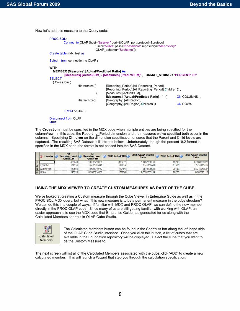
Now let’s add this measure to the Query code:

PROC SQL; Connect to OLAP (host="&server" port=&OLAP_port protocol=&protocol

user="&user" pass="&password" repository="&repository" OLAP_schema="&schema");

Create table mdx_test as Select * from connection to OLAP ( WITH MEMBER [Measures].[Actual/Predicted Ratio] As '[Measures].[ActualSUM] / [Measures].[PredictSUM]' , FORMAT_STRING = 'PERCENT10.2' SELECT { CrossJoin ( Hierarchize({ [Reporting_Period].[All Reporting_Period], [Reporting_Period].[All Reporting_Period].Children }) , { [Measures].[ActualSUM], [Measures].[Actual/Predicted Ratio] } ) } ON COLUMNS , Hierarchize({ [Geography].[All Region], [Geography].[All Region].Children }) ON ROWS FROM &cube. ); Disconnect from OLAP; Quit;

The CrossJoin must be specified in the MDX code when multiple entities are being specified for the column/row. In this case, the Reporting_Period dimension and the measures we’ve specified both occur in the columns. Specifying Children on the dimension specification ensures that the Parent and Child levels are captured. The resulting SAS Dataset is illustrated below. Unfortunately, though the percent10.2 format is specified in the MDX code, the format is not passed into the SAS Dataset.

USING THE MDX VIEWER TO CREATE CUSTOM MEASURES AS PART OF THE CUBE We’ve looked at creating a Custom measure through the Cube Viewer in Enterprise Guide as well as in the PROC SQL MDX query, but what if this new measure is to be a permanent measure in the cube structure? We can do this in a couple of ways. If familiar with MDX and PROC OLAP, we can define the new member directly in the PROC OLAP code. Since many of us are still getting familiar with working with OLAP, an easier approach is to use the MDX code that Enterprise Guide has generated for us along with the Calculated Members shortcut in OLAP Cube Studio.

The Calculated Members button can be found in the Shortcuts bar along the left hand side of the OLAP Cube Studio interface. Once you click this button, a list of cubes that are available in the Foundation repository will be displayed. Select the cube that you want to tie the Custom Measure to.

The next screen will list all of the Calculated Members associated with the cube; click ‘ADD’ to create a new calculated member. This will launch a Wizard that step you through the calculation specification.


9

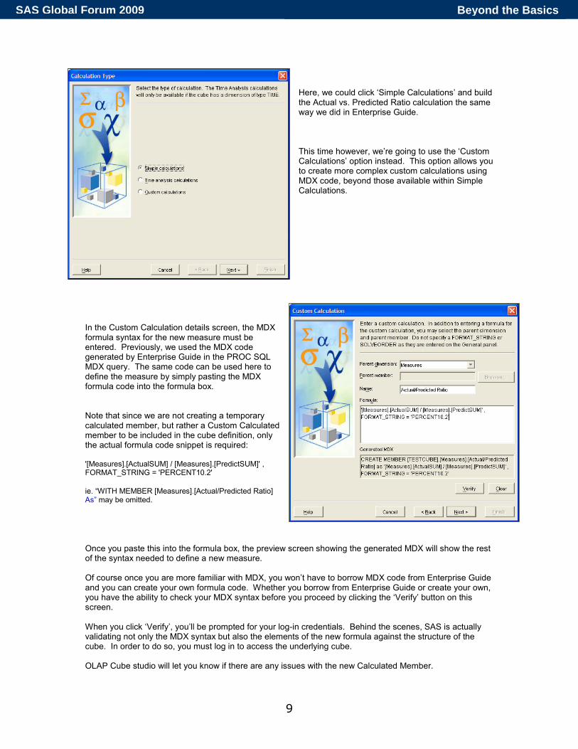
Here, we could click ‘Simple Calculations’ and build the Actual vs. Predicted Ratio calculation the same way we did in Enterprise Guide. This time however, we’re going to use the ‘Custom Calculations’ option instead. This option allows you to create more complex custom calculations using MDX code, beyond those available within Simple Calculations.

In the Custom Calculation details screen, the MDX formula syntax for the new measure must be entered. Previously, we used the MDX code generated by Enterprise Guide in the PROC SQL MDX query. The same code can be used here to define the measure by simply pasting the MDX formula code into the formula box. Note that since we are not creating a temporary calculated member, but rather a Custom Calculated member to be included in the cube definition, only the actual formula code snippet is required: '[Measures].[ActualSUM] / [Measures].[PredictSUM]' , FORMAT_STRING = 'PERCENT10.2'

ie. “WITH MEMBER [Measures].[Actual/Predicted Ratio] As” may be omitted.

Once you paste this into the formula box, the preview screen showing the generated MDX will show the rest of the syntax needed to define a new measure. Of course once you are more familiar with MDX, you won’t have to borrow MDX code from Enterprise Guide and you can create your own formula code. Whether you borrow from Enterprise Guide or create your own, you have the ability to check your MDX syntax before you proceed by clicking the ‘Verify’ button on this screen. When you click ‘Verify’, you’ll be prompted for your log-in credentials. Behind the scenes, SAS is actually validating not only the MDX syntax but also the elements of the new formula against the structure of the cube. In order to do so, you must log in to access the underlying cube. OLAP Cube studio will let you know if there are any issues with the new Calculated Member.


10

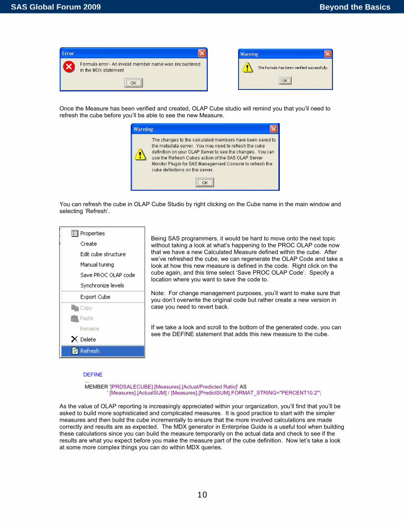
Once the Measure has been verified and created, OLAP Cube studio will remind you that you’ll need to refresh the cube before you’ll be able to see the new Measure. You can refresh the cube in OLAP Cube Studio by right clicking on the Cube name in the main window and selecting ‘Refresh’.

Being SAS programmers, it would be hard to move onto the next topic without taking a look at what’s happening to the PROC OLAP code now that we have a new Calculated Measure defined within the cube. After we’ve refreshed the cube, we can regenerate the OLAP Code and take a look at how this new measure is defined in the code. Right click on the cube again, and this time select ‘Save PROC OLAP Code’. Specify a location where you want to save the code to. Note: For change management purposes, you’ll want to make sure that you don’t overwrite the original code but rather create a new version in case you need to revert back. If we take a look and scroll to the bottom of the generated code, you can see the DEFINE statement that adds this new measure to the cube.

DEFINE ... MEMBER '[PRDSALECUBE].[Measures].[Actual/Predicted Ratio]' AS

' [Measures].[ActualSUM] / [Measures].[PredictSUM],FORMAT_STRING="PERCENT10.2"';

As the value of OLAP reporting is increasingly appreciated within your organization, you’ll find that you’ll be asked to build more sophisticated and complicated measures. It is good practice to start with the simpler measures and then build the cube incrementally to ensure that the more involved calculations are made correctly and results are as expected. The MDX generator in Enterprise Guide is a useful tool when building these calculations since you can build the measure temporarily on the actual data and check to see if the results are what you expect before you make the measure part of the cube definition. Now let’s take a look at some more complex things you can do within MDX queries.


11

SOME HANDY MDX FUNCTIONS FOR YOUR QUERIES

PERIODSTODATE()

You’ll often be asked to report data based on some sort of time series analysis such as month over month performance or time based trending. To support this type of analysis, MDX has a group of built in time series functions that allow you to extract data or define groups based on time and date characteristics. One of the most useful functions in this group is the PeriodsToDate() function.

Syntax: PeriodsToDate([<Level>[,<member>]])

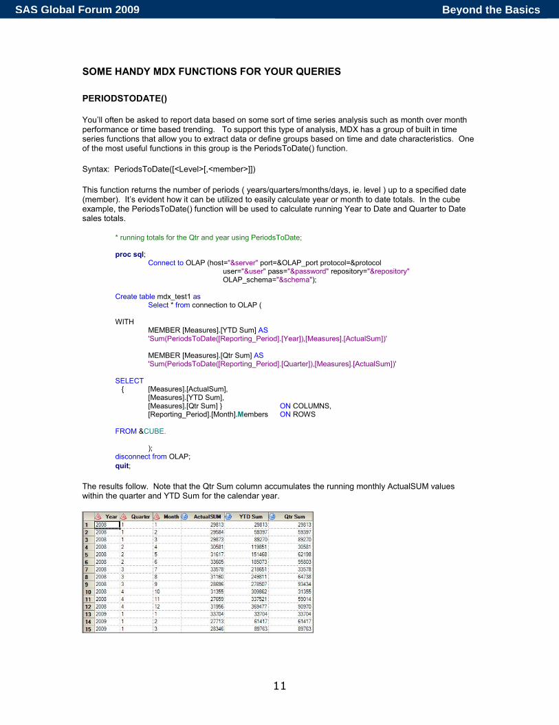
This function returns the number of periods ( years/quarters/months/days, ie. level ) up to a specified date (member). It’s evident how it can be utilized to easily calculate year or month to date totals. In the cube example, the PeriodsToDate() function will be used to calculate running Year to Date and Quarter to Date sales totals.

* running totals for the Qtr and year using PeriodsToDate; proc sql; Connect to OLAP (host="&server" port=&OLAP_port protocol=&protocol


Create table mdx_test1 as Select * from connection to OLAP ( WITH MEMBER [Measures].[YTD Sum] AS 'Sum(PeriodsToDate([Reporting_Period].[Year]),[Measures].[ActualSum])' MEMBER [Measures].[Qtr Sum] AS 'Sum(PeriodsToDate([Reporting_Period].[Quarter]),[Measures].[ActualSum])' SELECT { [Measures].[ActualSum],

[Measures].[YTD Sum], [Measures].[Qtr Sum] } ON COLUMNS, [Reporting_Period].[Month].Members ON ROWS FROM &CUBE. ); disconnect from OLAP;

quit;

The results follow. Note that the Qtr Sum column accumulates the running monthly ActualSUM values within the quarter and YTD Sum for the calendar year.


12

Try it: Another time series function worth exploring is the ParallelPeriod() function. This allows you to compare the current period to the previous relative period. For example, you could compare February 2008 to February 2007 or Quarter 1 2008 and Quarter 1 2007.

BOTTOMCOUNT()

The BottomCount() function allows us to query through any number of specified members in a cube and pull out the lowest ranking members for a given numeric value expression. This is a very useful function since it allows us to quickly identify members that may be under-performing in terms of having the lowest sales or over-performing in terms of lowest returns.

Syntax: BottomCount(<Set>, <Count> [,<Numeric Expression/Measure>])

BottomCount() essentially sorts a set based on the measure or expression provided and then returns the bottom <count> number of items.

Building on the previous example, we’re now interested in identifying the three regions with the lowest Year to Date sales as of the 3

rd quarter in 2008. Note the inclusion of the WHERE clause to specify the date

criteria. The Hierarchize function organizes the members of specified set into hierarchical order. The Descendants function returns the set of descendants within the Geography hierarchy, not just the lowest level, Region, that would otherwise result.

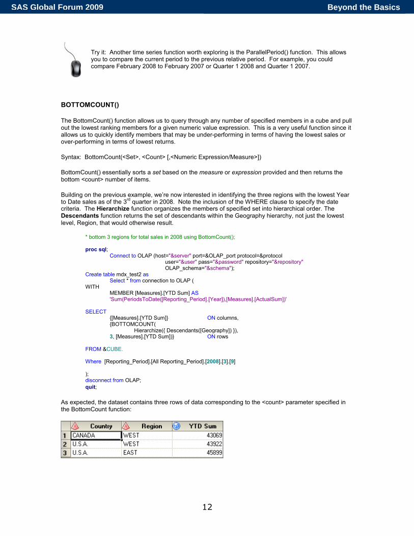
* bottom 3 regions for total sales in 2008 using BottomCount(); proc sql; Connect to OLAP (host="&server" port=&OLAP_port protocol=&protocol


Create table mdx_test2 as Select * from connection to OLAP ( WITH MEMBER [Measures].[YTD Sum] AS 'Sum(PeriodsToDate([Reporting_Period].[Year]),[Measures].[ActualSum])' SELECT {[Measures].[YTD Sum]} ON columns, {BOTTOMCOUNT( Hierarchize({ Descendants([Geography]) }), 3, [Measures].[YTD Sum])} ON rows FROM &CUBE. Where [Reporting_Period].[All Reporting_Period].[2008].[3].[9] ); disconnect from OLAP;

quit;

As expected, the dataset contains three rows of data corresponding to the <count> parameter specified in the BottomCount function:


13

Try it: A variation of this function is the TopCount() function which as you may have guessed, allows you to select the top ranking members of a set based on a numeric expression or measure.

IIF()

The IIF() function allows you to return one of two possible values based on the results of the specified logical test. This can come in handy when querying a cube and when creating a custom measure or member.

Syntax: IIF(<logical expression>, <Numeric or String Expression 1>, <Numeric of String Expression2> )

If the logical expression is true, the function will return the value of the Numeric or String Expression 1. Otherwise it returns the value of the second Numeric or String expression.

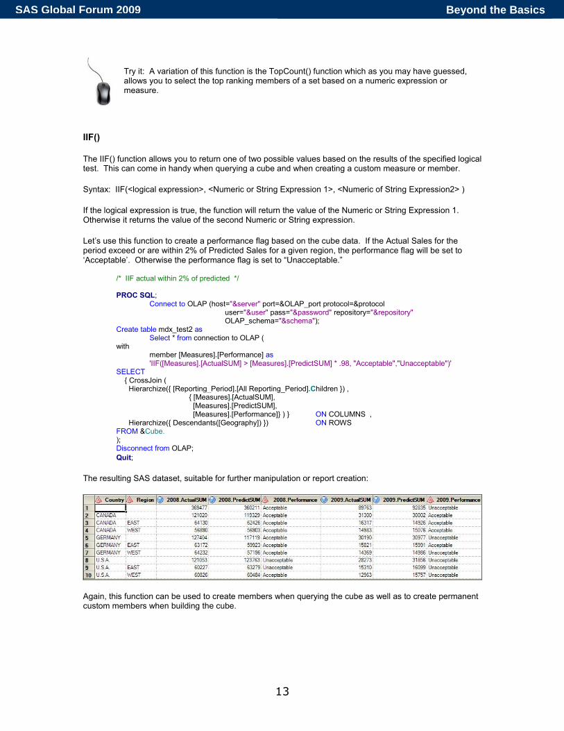
Let’s use this function to create a performance flag based on the cube data. If the Actual Sales for the period exceed or are within 2% of Predicted Sales for a given region, the performance flag will be set to ‘Acceptable’. Otherwise the performance flag is set to “Unacceptable.”

/* IIF actual within 2% of predicted */ PROC SQL; Connect to OLAP (host="&server" port=&OLAP_port protocol=&protocol


Create table mdx_test2 as Select * from connection to OLAP ( with

member [Measures].[Performance] as 'IIF([Measures].[ActualSUM] > [Measures].[PredictSUM] * .98, "Acceptable","Unacceptable")'

SELECT { CrossJoin ( Hierarchize({ [Reporting_Period].[All Reporting_Period].Children }) , { [Measures].[ActualSUM], [Measures].[PredictSUM], [Measures].[Performance]} ) } ON COLUMNS , Hierarchize({ Descendants([Geography]) }) ON ROWS FROM &Cube. ); Disconnect from OLAP;

Quit;

The resulting SAS dataset, suitable for further manipulation or report creation:

Again, this function can be used to create members when querying the cube as well as to create permanent custom members when building the cube.


14

USING SAS FUNCTIONS WITHIN MDX

While MDX supports a wide range of useful functions, there may be times where you need to call a SAS function to fulfill reporting requirements. For example, you may want to run a report that looks at Sales totals for a given month.

In a previous MDX example, we looked at the three worst performing regions in 2008 by Sales to Date. What if we wanted to automatically create a report each month that looked at the three worst performing regions for that month? There are a few ways that we can do this. We could pull all the data from the cube and then use a subsequent step to filter based on the date that we’re interested in. However, this wouldn’t be optimal since unnecessary data would be pulled and multiple passes through the data would be inefficient. We could also hard-code the dates in the MDX query code so that we’re only pulling data for the dates that we’re interested in. While this is a better option than the first, since this report will run every month, we have to think about program maintenance and an automated solution. The solution is to embed the appropriate SAS date functions in the MDX query so that the three worst performing regions are pulled for the current month.

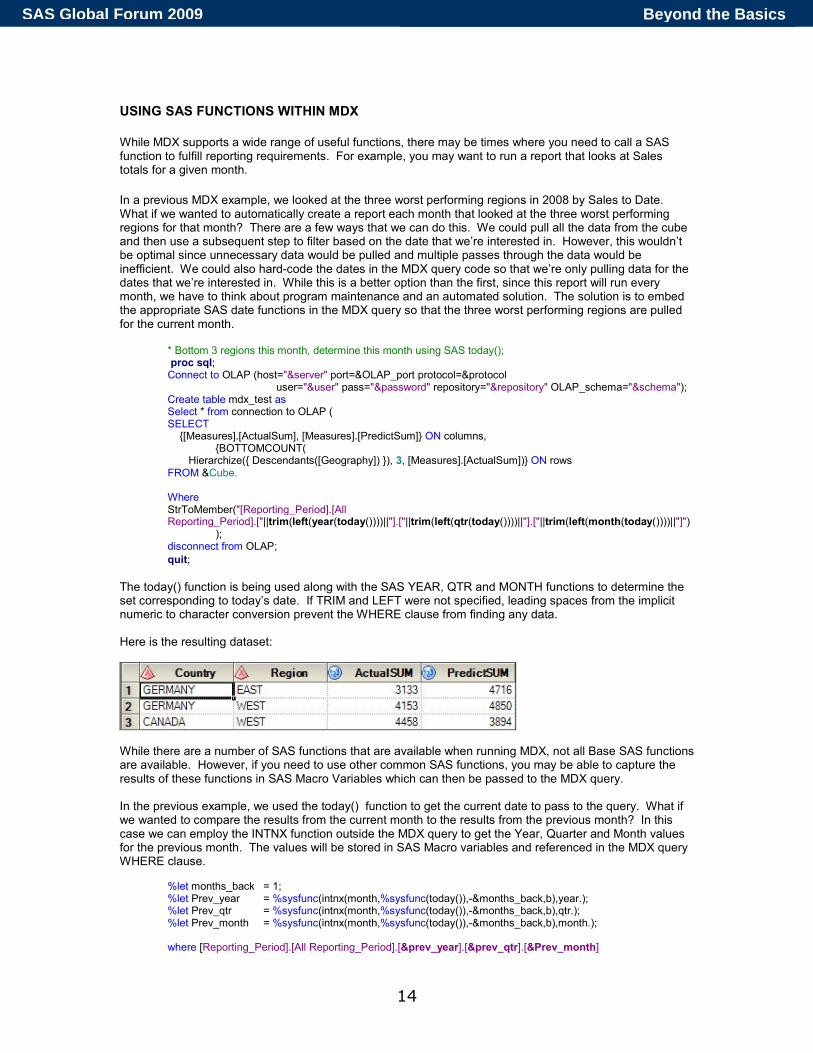
* Bottom 3 regions this month, determine this month using SAS today(); proc sql; Connect to OLAP (host="&server" port=&OLAP_port protocol=&protocol

user="&user" pass="&password" repository="&repository" OLAP_schema="&schema"); Create table mdx_test as Select * from connection to OLAP ( SELECT {[Measures].[ActualSum], [Measures].[PredictSum]} ON columns, {BOTTOMCOUNT( Hierarchize({ Descendants([Geography]) }), 3, [Measures].[ActualSum])} ON rows FROM &Cube. Where StrToMember("[Reporting_Period].[All Reporting_Period].["||trim(left(year(today())))||"].["||trim(left(qtr(today())))||"].["||trim(left(month(today())))||"]") ); disconnect from OLAP;

quit;

The today() function is being used along with the SAS YEAR, QTR and MONTH functions to determine the set corresponding to today’s date. If TRIM and LEFT were not specified, leading spaces from the implicit numeric to character conversion prevent the WHERE clause from finding any data. Here is the resulting dataset:

While there are a number of SAS functions that are available when running MDX, not all Base SAS functions are available. However, if you need to use other common SAS functions, you may be able to capture the results of these functions in SAS Macro Variables which can then be passed to the MDX query. In the previous example, we used the today() function to get the current date to pass to the query. What if we wanted to compare the results from the current month to the results from the previous month? In this case we can employ the INTNX function outside the MDX query to get the Year, Quarter and Month values for the previous month. The values will be stored in SAS Macro variables and referenced in the MDX query WHERE clause.

%let months_back = 1; %let Prev_year = %sysfunc(intnx(month,%sysfunc(today()),-&months_back,b),year.); %let Prev_qtr = %sysfunc(intnx(month,%sysfunc(today()),-&months_back,b),qtr.); %let Prev_month = %sysfunc(intnx(month,%sysfunc(today()),-&months_back,b),month.); where [Reporting_Period].[All Reporting_Period].[&prev_year].[&prev_qtr].[&Prev_month]


15

The results for the previous month will be returned which enables comparison to the current month’s figures. Since the SAS Macro variables are simply substituted into the query as text, the StrToMember function used in the previous “today()” example is unnecessary. It should be noted that as of version 9.2, all Base SAS functions will be available for use in MDX queries, as well as a select number from SAS/STAT, SAS/ETS and SAS/OR.

Try it: Another interesting and helpful use of embedding SAS in MDX is that you can use the PUT function to apply standard SAS formats as well as user-defined formats to the cube data.

CREATING MULTIPLE DEPENDENT MEASURES IN A SINGLE QUERY So far we’ve looked at using MDX to:

• create running YTD and QTD sales totals using PeriodsToDate

• identify the weakest regions using BottomCount

• identify performing and non-performing regions using IIF and simple calculated ratios. In this last example, we’re going to tie some of these concepts together within a single query. As in the previous examples, we want to get a running YTD and QTD total but this time we want to look at how Actual Sales compare to Predicted Sales as the year progressed. To readily highlight ongoing performance for folks who don’t care to look too closely at the numbers, we also want to generate Acceptable and Unacceptable performance flags (based on the YTD and QTD running totals ) on a monthly basis. Finally, we want to break down performance by Product and the Time dimension periods. In order to meet these requirements, we’ll need to create the calculated measures in several steps: Step 1 - calculate the QTD and LTD running totals for Actual and Predicted Sales; Step 2 - calculate the Actual/Predicted Ratio based on the QTD and YTD running totals from Step 1; Step 3 - set the Performance Flags based on the Actual/Predicted ratios from Step 2. To ensure the measures are calculated in the correct sequence, we must specify the computation order via the ‘solve_order’ option in the MDX query. OLAP cube measures are calculated via a number of stages or ‘Calculation Passes’. Within the context of calculated measures, ‘Solve_Order’ determines the order in which calculated measures will be evaluated for each ‘calculation pass’. In the example, the running totals have a solve order of 1 so they will be computed first. The Actual/Predicted ratios will have a solve order of 2, so these will be computed once the running totals have been calculated. Finally, since the Performance Flag depends on the other two calculations, it has a solve order of 3 making it the last calculated measure to be processed. Here is the query needed to obtain the results. Note that the Product Dimension has been CrossJoined to the Reporting Period dimension since the additional breakdown is required for the analysis. AllMembers has been specified on the Product Type dimension to ensure all levels were provided.

* Tying it all together, running totals for the Qtr and Yr, Actual/Predicted Ratio, introducing Solve Order; proc sql; Connect to OLAP <snip> Create table mdx_test as Select * from connection to OLAP ( WITH MEMBER [Measures].[Qtr Actual Sum] AS

'Sum(PeriodsToDate([Reporting_Period].[Quarter]),[Measures].[ActualSum]), solve_order=1' MEMBER [Measures].[YTD Actual Sum] AS

'Sum(PeriodsToDate([Reporting_Period].[Year]),[Measures].[ActualSum]), solve_order=1'


16

MEMBER [Measures].[Qtr Pred Sum] AS 'Sum(PeriodsToDate([Reporting_Period].[Quarter]),[Measures].[PredictSum]), solve_order=1'

MEMBER [Measures].[YTD Pred Sum] AS

'Sum(PeriodsToDate([Reporting_Period].[Year]),[Measures].[PredictSum]), solve_order=1' MEMBER [Measures].[QTR Actual/Predicted Ratio] as

'[Measures].[Qtr Actual Sum] / [Measures].[Qtr Pred Sum], format_string="Percent", solve_order=2' MEMBER [Measures].[YTD Actual/Predicted Ratio] as

'[Measures].[YTD Actual Sum] / [Measures].[YTD Pred Sum], format_string="Percent", solve_order=2'

MEMBER [Measures].[YTD Performance] as 'IIF([Measures].[YTD Actual/Predicted Ratio] > .98, "Acceptable","Unacceptable"), solve_order=3'

MEMBER [Measures].[QTD Performance] as

'IIF([Measures].[QTR Actual/Predicted Ratio] > .98, "Acceptable","Unacceptable"), solve_order=3'

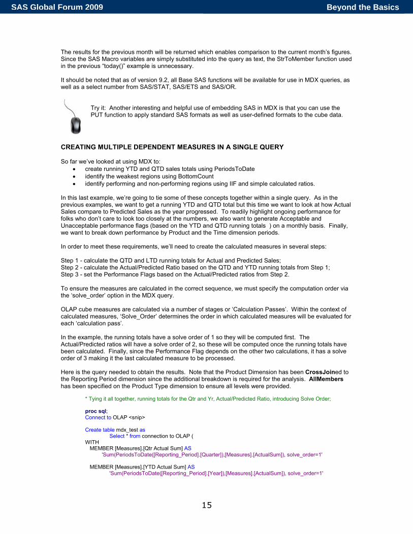
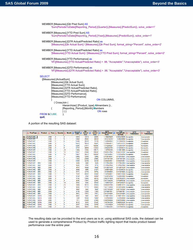
SELECT {[Measures].[ActualSum], [Measures].[Qtr Actual Sum], [Measures].[YTD Actual Sum], [Measures].[QTR Actual/Predicted Ratio], [Measures].[YTD Actual/Predicted Ratio], [Measures].[QTD Performance], [Measures].[YTD Performance] } ON COLUMNS, { CrossJoin ( Hierarchize({ [Product_type].Allmembers }) , { [Reporting_Period].[Month].Members } ) } ON rows FROM &CUBE. ); quit;

A portion of the resulting SAS dataset:

The resulting data can be provided to the end users as is or, using additional SAS code, the dataset can be used to generate a comprehensive Product by Product traffic lighting report that tracks product based performance over the entire year.


17

CONCLUSION OLAP cubes are quickly becoming indispensable in dealing with the burgeoning quantity of corporate data. The multidimensional view of aggregated data that OLAP provides affords quick and easy access to the analysis data required to make sound business decisions. It’s evident how useful Multidimensional Expression Language ( MDX ) can be for manipulating and surfacing OLAP cube data. While the MDX syntax certainly appears complex initially, Enterprise Guide’s MDX editor display is helpful in reducing the learning curve. The examples provided will allow you to customize your OLAP cube report data and leverage the potential analytical insights for your business needs.

REFERENCES

• http://msdn.microsoft.com/en-us/library/ - MDX Reference

• http://mdxpert.com/ - MDX-pert

• http://support.sas.com/documentation/onlinedoc/91pdf/sasdoc_913/OLAP_mdx_9317.pdf - SAS 9.1.3 OLAP

Server: MDX Guide

ACKNOWLEDGMENTS

• Adam Budlong – SAS Technical Support

RECOMMENDED READING

• http://www2.sas.com/proceedings/sugi31/219-31.pdf - Beyond the Basics: Advanced OLAP Techniques, Ben

Zenick and Brian Miles

• http://www2.sas.com/proceedings/forum2008/182-2008.pdf - Building OLAP Cubes with SAS 9, Gregory Nelson

• http://www2.sas.com/proceedings/forum2008/044-2008.pdf - Exploring OLAP Cubes with Enterprise Guide,

Rupinder Dhillon

CONTACT INFORMATION

Your comments and questions are valued and encouraged. Contact the authors at:

Rupinder Dhillon Dhillon Consulting Inc. 12 Givins St. Toronto, ON M6J 2X6 (416) 220 9191 [email protected] www.dhillonconsulting.com

Harry Droogendyk Stratia Consulting Inc. PO Box 145 Lynden, ON L0R 1T0 [email protected] www.stratia.ca

SAS and all other SAS Institute Inc. product or service names are registered trademarks or trademarks of SAS Institute

Inc. in the USA and other countries. ® indicates USA registration.

Other brand and product names are trademarks of their respective companies.


18

APPENDIX

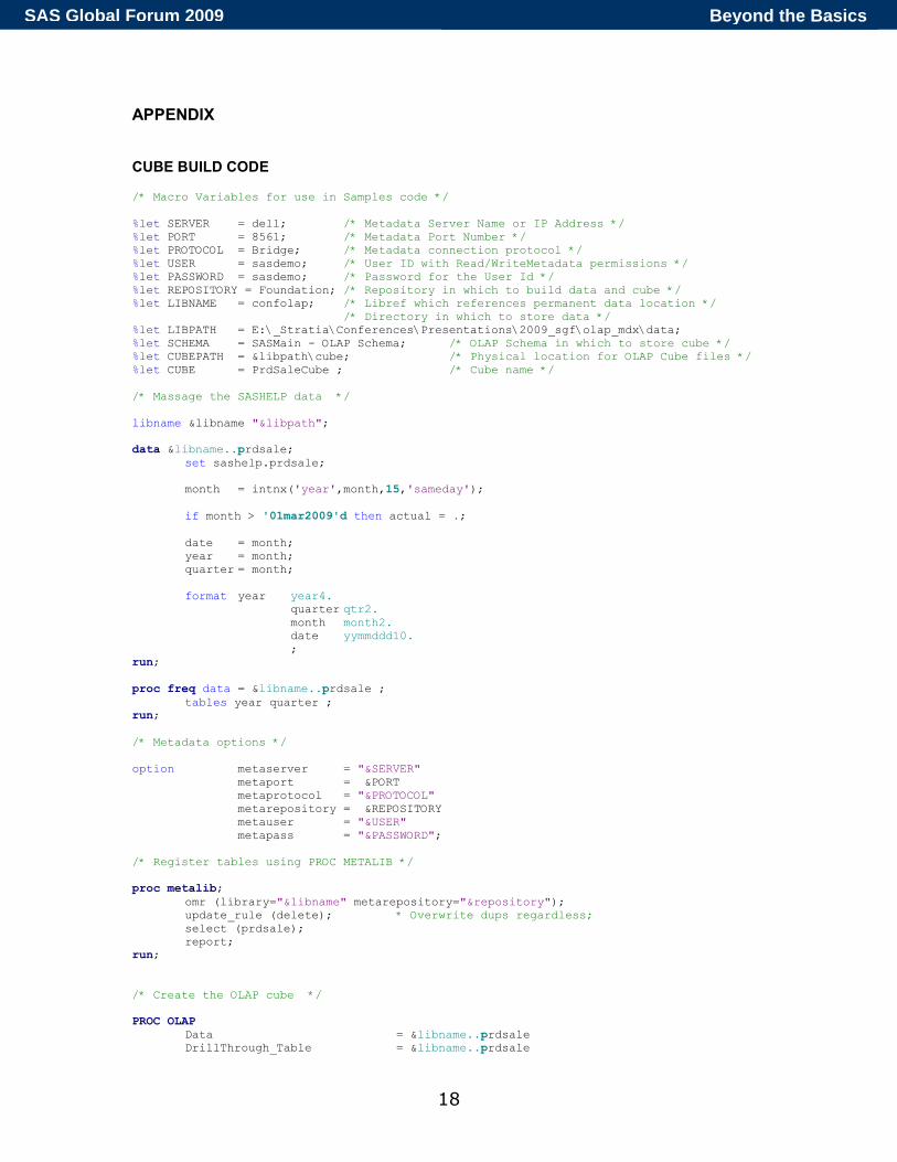
CUBE BUILD CODE /* Macro Variables for use in Samples code */ %let SERVER = dell; /* Metadata Server Name or IP Address */ %let PORT = 8561; /* Metadata Port Number */ %let PROTOCOL = Bridge; /* Metadata connection protocol */ %let USER = sasdemo; /* User ID with Read/WriteMetadata permissions */ %let PASSWORD = sasdemo; /* Password for the User Id */ %let REPOSITORY = Foundation; /* Repository in which to build data and cube */ %let LIBNAME = confolap; /* Libref which references permanent data location */ /* Directory in which to store data */ %let LIBPATH = E:\_Stratia\Conferences\Presentations\2009_sgf\olap_mdx\data; %let SCHEMA = SASMain - OLAP Schema; /* OLAP Schema in which to store cube */ %let CUBEPATH = &libpath\cube; /* Physical location for OLAP Cube files */ %let CUBE = PrdSaleCube ; /* Cube name */ /* Massage the SASHELP data */ libname &libname "&libpath"; data &libname..prdsale; set sashelp.prdsale; month = intnx('year',month,15,'sameday'); if month > '01mar2009'd then actual = .; date = month; year = month; quarter = month; format year year4. quarter qtr2. month month2. date yymmddd10. ; run; proc freq data = &libname..prdsale ; tables year quarter ; run; /* Metadata options */ option metaserver = "&SERVER" metaport = &PORT metaprotocol = "&PROTOCOL" metarepository = &REPOSITORY metauser = "&USER" metapass = "&PASSWORD"; /* Register tables using PROC METALIB */ proc metalib; omr (library="&libname" metarepository="&repository"); update_rule (delete); * Overwrite dups regardless; select (prdsale); report; run; /* Create the OLAP cube */ PROC OLAP Data = &libname..prdsale DrillThrough_Table = &libname..prdsale


19

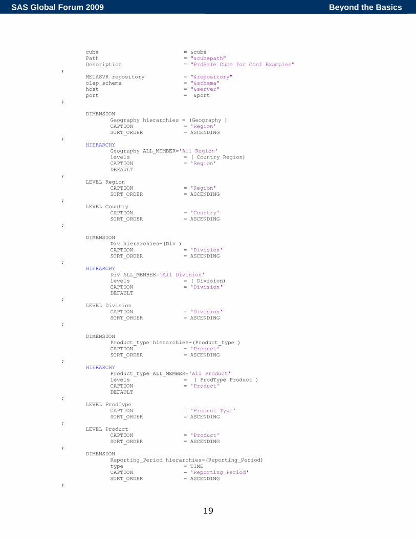
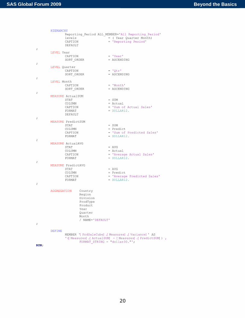
cube = &cube Path = "&cubepath" Description = "PrdSale Cube for Conf Examples" ; METASVR repository = "&repository"

olap_schema = "&schema" host = "&server" port = &port ; DIMENSION Geography hierarchies = (Geography ) CAPTION = 'Region' SORT_ORDER = ASCENDING ; HIERARCHY Geography ALL_MEMBER='All Region' levels = ( Country Region) CAPTION = 'Region' DEFAULT ; LEVEL Region CAPTION = 'Region' SORT_ORDER = ASCENDING ; LEVEL Country CAPTION = 'Country' SORT_ORDER = ASCENDING ; DIMENSION Div hierarchies=(Div ) CAPTION = 'Division' SORT_ORDER = ASCENDING ; HIERARCHY Div ALL_MEMBER='All Division' levels = ( Division) CAPTION = 'Division' DEFAULT ; LEVEL Division CAPTION = 'Division' SORT_ORDER = ASCENDING ; DIMENSION Product_type hierarchies=(Product_type ) CAPTION = 'Product' SORT_ORDER = ASCENDING ; HIERARCHY Product_type ALL_MEMBER='All Product' levels = ( ProdType Product ) CAPTION = 'Product' DEFAULT ; LEVEL ProdType CAPTION = 'Product Type' SORT_ORDER = ASCENDING ; LEVEL Product CAPTION = 'Product' SORT_ORDER = ASCENDING ; DIMENSION Reporting_Period hierarchies=(Reporting_Period) type = TIME CAPTION = 'Reporting Period' SORT_ORDER = ASCENDING ;


20

HIERARCHY Reporting_Period ALL_MEMBER='All Reporting_Period' levels = ( Year Quarter Month) CAPTION = 'Reporting Period' DEFAULT ; LEVEL Year CAPTION = 'Year' SORT_ORDER = ASCENDING ; LEVEL Quarter CAPTION = 'Qtr' SORT_ORDER = ASCENDING ; LEVEL Month CAPTION = 'Month' SORT_ORDER = ASCENDING ; MEASURE ActualSUM STAT = SUM COLUMN = Actual CAPTION = 'Sum of Actual Sales' FORMAT = DOLLAR12. DEFAULT ; MEASURE PredictSUM STAT = SUM COLUMN = Predict CAPTION = 'Sum of Predicted Sales' FORMAT = DOLLAR12. ; MEASURE ActualAVG STAT = AVG COLUMN = Actual CAPTION = 'Average Actual Sales' FORMAT = DOLLAR12. ; MEASURE PredictAVG STAT = AVG COLUMN = Predict CAPTION = 'Average Predicted Sales' FORMAT = DOLLAR12. ;

AGGREGATION Country Region

Division ProdType Product Year Quarter Month / NAME='DEFAULT' ; DEFINE MEMBER '[PrdSaleCube].[Measures].[Variance]' AS '([Measures].[ActualSUM] - [Measures].[PredictSUM]) ,

FORMAT_STRING = "dollar30."'; RUN;


21

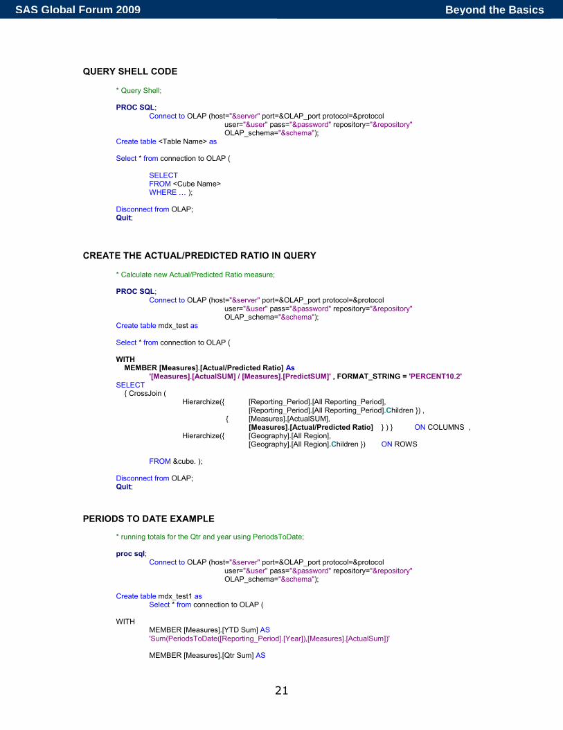
QUERY SHELL CODE

* Query Shell; PROC SQL; Connect to OLAP (host="&server" port=&OLAP_port protocol=&protocol


Create table <Table Name> as Select * from connection to OLAP (

SELECT FROM <Cube Name>

WHERE … ); Disconnect from OLAP; Quit;

CREATE THE ACTUAL/PREDICTED RATIO IN QUERY

* Calculate new Actual/Predicted Ratio measure; PROC SQL; Connect to OLAP (host="&server" port=&OLAP_port protocol=&protocol


Create table mdx_test as Select * from connection to OLAP ( WITH MEMBER [Measures].[Actual/Predicted Ratio] As '[Measures].[ActualSUM] / [Measures].[PredictSUM]' , FORMAT_STRING = 'PERCENT10.2' SELECT { CrossJoin ( Hierarchize({ [Reporting_Period].[All Reporting_Period], [Reporting_Period].[All Reporting_Period].Children }) , { [Measures].[ActualSUM], [Measures].[Actual/Predicted Ratio] } ) } ON COLUMNS , Hierarchize({ [Geography].[All Region], [Geography].[All Region].Children }) ON ROWS FROM &cube. ); Disconnect from OLAP; Quit;

PERIODS TO DATE EXAMPLE * running totals for the Qtr and year using PeriodsToDate; proc sql; Connect to OLAP (host="&server" port=&OLAP_port protocol=&protocol


Create table mdx_test1 as Select * from connection to OLAP ( WITH MEMBER [Measures].[YTD Sum] AS 'Sum(PeriodsToDate([Reporting_Period].[Year]),[Measures].[ActualSum])' MEMBER [Measures].[Qtr Sum] AS


22

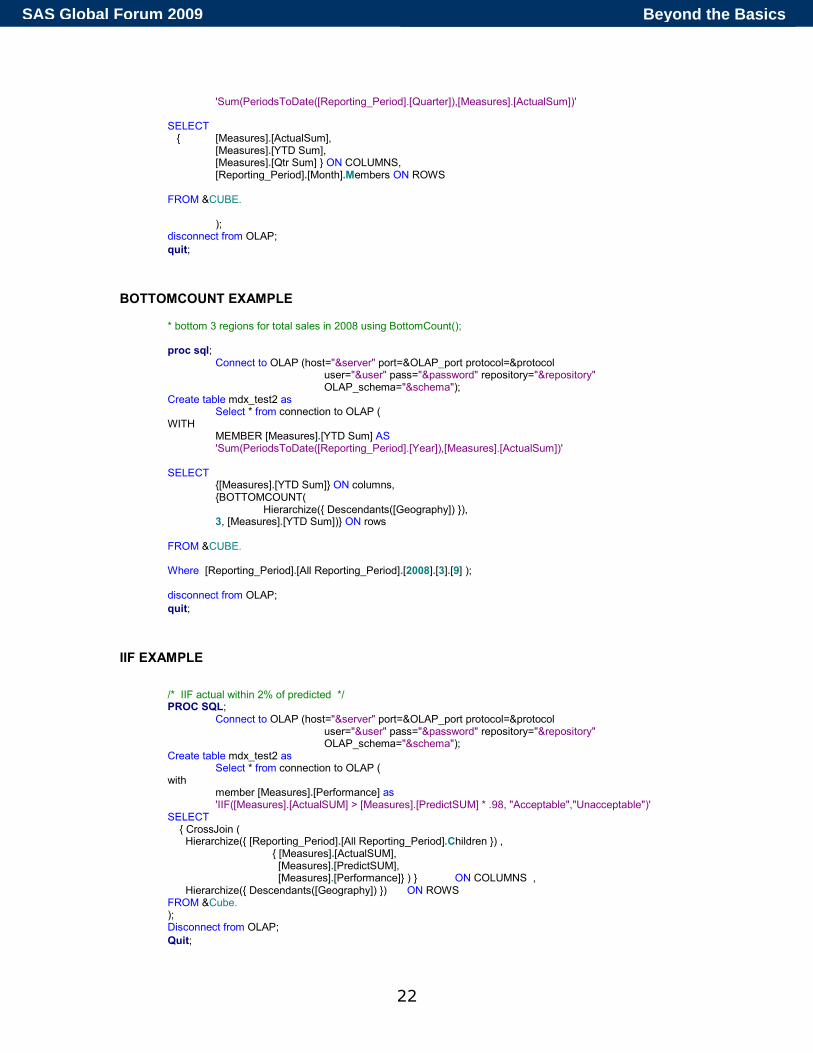
'Sum(PeriodsToDate([Reporting_Period].[Quarter]),[Measures].[ActualSum])' SELECT { [Measures].[ActualSum],

[Measures].[YTD Sum], [Measures].[Qtr Sum] } ON COLUMNS, [Reporting_Period].[Month].Members ON ROWS FROM &CUBE. ); disconnect from OLAP;

quit;

BOTTOMCOUNT EXAMPLE * bottom 3 regions for total sales in 2008 using BottomCount(); proc sql; Connect to OLAP (host="&server" port=&OLAP_port protocol=&protocol


Create table mdx_test2 as Select * from connection to OLAP ( WITH MEMBER [Measures].[YTD Sum] AS 'Sum(PeriodsToDate([Reporting_Period].[Year]),[Measures].[ActualSum])' SELECT {[Measures].[YTD Sum]} ON columns, {BOTTOMCOUNT( Hierarchize({ Descendants([Geography]) }), 3, [Measures].[YTD Sum])} ON rows FROM &CUBE. Where [Reporting_Period].[All Reporting_Period].[2008].[3].[9] ); disconnect from OLAP;

quit;

IIF EXAMPLE

/* IIF actual within 2% of predicted */ PROC SQL; Connect to OLAP (host="&server" port=&OLAP_port protocol=&protocol


Create table mdx_test2 as Select * from connection to OLAP ( with

member [Measures].[Performance] as 'IIF([Measures].[ActualSUM] > [Measures].[PredictSUM] * .98, "Acceptable","Unacceptable")'

SELECT { CrossJoin ( Hierarchize({ [Reporting_Period].[All Reporting_Period].Children }) , { [Measures].[ActualSUM], [Measures].[PredictSUM], [Measures].[Performance]} ) } ON COLUMNS , Hierarchize({ Descendants([Geography]) }) ON ROWS FROM &Cube. ); Disconnect from OLAP;

Quit;


23

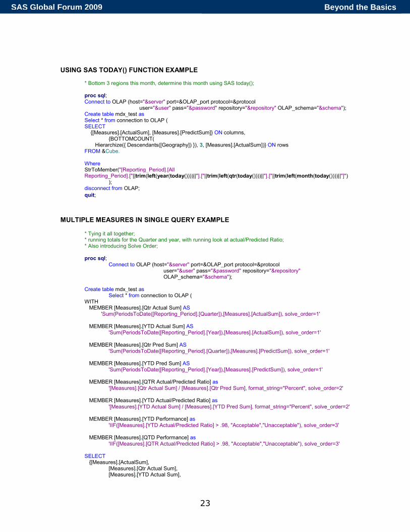
USING SAS TODAY() FUNCTION EXAMPLE * Bottom 3 regions this month, determine this month using SAS today(); proc sql; Connect to OLAP (host="&server" port=&OLAP_port protocol=&protocol

user="&user" pass="&password" repository="&repository" OLAP_schema="&schema"); Create table mdx_test as Select * from connection to OLAP ( SELECT {[Measures].[ActualSum], [Measures].[PredictSum]} ON columns, {BOTTOMCOUNT( Hierarchize({ Descendants([Geography]) }), 3, [Measures].[ActualSum])} ON rows FROM &Cube. Where StrToMember("[Reporting_Period].[All Reporting_Period].["||trim(left(year(today())))||"].["||trim(left(qtr(today())))||"].["||trim(left(month(today())))||"]") ); disconnect from OLAP;

quit;

MULTIPLE MEASURES IN SINGLE QUERY EXAMPLE

* Tying it all together; * running totals for the Quarter and year, with running look at actual/Predicted Ratio; * Also introducing Solve Order; proc sql; Connect to OLAP (host="&server" port=&OLAP_port protocol=&protocol


Create table mdx_test as Select * from connection to OLAP ( WITH MEMBER [Measures].[Qtr Actual Sum] AS

'Sum(PeriodsToDate([Reporting_Period].[Quarter]),[Measures].[ActualSum]), solve_order=1' MEMBER [Measures].[YTD Actual Sum] AS

'Sum(PeriodsToDate([Reporting_Period].[Year]),[Measures].[ActualSum]), solve_order=1' MEMBER [Measures].[Qtr Pred Sum] AS

'Sum(PeriodsToDate([Reporting_Period].[Quarter]),[Measures].[PredictSum]), solve_order=1' MEMBER [Measures].[YTD Pred Sum] AS

'Sum(PeriodsToDate([Reporting_Period].[Year]),[Measures].[PredictSum]), solve_order=1' MEMBER [Measures].[QTR Actual/Predicted Ratio] as

'[Measures].[Qtr Actual Sum] / [Measures].[Qtr Pred Sum], format_string="Percent", solve_order=2' MEMBER [Measures].[YTD Actual/Predicted Ratio] as

'[Measures].[YTD Actual Sum] / [Measures].[YTD Pred Sum], format_string="Percent", solve_order=2'

MEMBER [Measures].[YTD Performance] as 'IIF([Measures].[YTD Actual/Predicted Ratio] > .98, "Acceptable","Unacceptable"), solve_order=3'

MEMBER [Measures].[QTD Performance] as

'IIF([Measures].[QTR Actual/Predicted Ratio] > .98, "Acceptable","Unacceptable"), solve_order=3'

SELECT {[Measures].[ActualSum], [Measures].[Qtr Actual Sum], [Measures].[YTD Actual Sum],


24

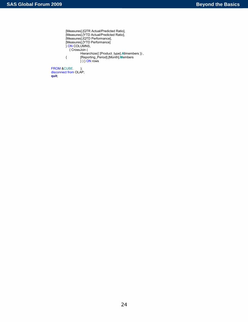
[Measures].[QTR Actual/Predicted Ratio], [Measures].[YTD Actual/Predicted Ratio], [Measures].[QTD Performance], [Measures].[YTD Performance] } ON COLUMNS, { CrossJoin ( Hierarchize({ [Product_type].Allmembers }) , { [Reporting_Period].[Month].Members } ) } ON rows FROM &CUBE. ); disconnect from OLAP; quit;


042-2009: Manipulating OLAP Cubes: Advanced Techniques...

Documents

Transcript of 042-2009: Manipulating OLAP Cubes: Advanced Techniques...