034758

Hindawi Publishing CorporationEURASIP Journal on Wireless Communications and NetworkingVolume 2007, Article ID 34758, 13 pagesdoi:10.1155/2007/34758

Research ArticleScalable Coverage Maintenance forDense Wireless Sensor Networks

Jun Lu, Jinsu Wang, and Tatsuya Suda

Bren School of Information and Computer Sciences, University of California, Irvine, CA 92697, USA

Received 1 October 2006; Accepted 30 March 2007

Recommended by Mischa Dohler

Owing to numerous potential applications, wireless sensor networks have been attracting significant research effort recently. Thecritical challenge that wireless sensor networks often face is to sustain long-term operation on limited battery energy. Coveragemaintenance schemes can effectively prolong network lifetime by selecting and employing a subset of sensors in the network toprovide sufficient sensing coverage over a target region. We envision future wireless sensor networks composed of a vast numberof miniaturized sensors in exceedingly high density. Therefore, the key issue of coverage maintenance for future sensor networksis the scalability to sensor deployment density. In this paper, we propose a novel coverage maintenance scheme, scalable coveragemaintenance (SCOM), which is scalable to sensor deployment density in terms of communication overhead (i.e., number of trans-mitted and received beacons) and computational complexity (i.e., time and space complexity). In addition, SCOM achieves highenergy efficiency and load balancing over different sensors. We have validated our claims through both analysis and simulations.

Copyright © 2007 Jun Lu et al. This is an open access article distributed under the Creative Commons Attribution License, whichpermits unrestricted use, distribution, and reproduction in any medium, provided the original work is properly cited.

1. INTRODUCTION

The recent advances in microsensor and communicationtechnologies have increased the possibility of manufactur-ing inexpensive small wireless sensors with simple sensing,processing, and wireless communication capabilities. Lim-ited by their size, small wireless sensors are equipped witha restricted power source and storage capacity. For example,the typical Crossbow MICA2 mote MPR400CB [1] has a low-speed 16 MHz microcontroller equipped with only 128 KBflash and 4 KB EEPROM. Powered by two AA batteries, ithas the maximal data rate of 38.4 KBaud and a transmissionrange of about 150 m. Such small wireless sensors are usu-ally deployed in an ad hoc manner to monitor a specified re-gion of interest for various applications such as environmentmonitoring, target tracking, and distributed data storage.

One fundamental problem faced by current sensor net-work deployment is efficient provision of the required cover-age. Specifically, given a target region, how can it guaranteethat every point in the region is covered by the required num-ber of sensors, with the object of maximizing the lifetime ofthe whole network? This problem is challenging due to thelimitation of wireless sensor capabilities as well as the ad-hocdeployment properties of wireless sensor networks. One ef-

fective approach to extend sensor network lifetime is to havesensors autonomously schedule their duty cycles accordingto local information while satisfying global coverage require-ments, which is referred to as coverage maintenance in theliterature. We envision future wireless sensor networks com-posed of a vast number of small wireless sensors with verylimited processing capability and storage capacity in exceed-ingly high density [2, 3]. Therefore, coverage maintenancefor future wireless sensor networks must be highly scalable tosensor deployment density in terms of communication over-head as well as computational complexity.

In this paper, we propose a novel coverage maintenancescheme, scalable coverage maintenance (SCOM), in whichsensors decide their sensing states in a distributive man-ner. SCOM works in two phases—the decision phase andthe optimization phase. In the decision phase, sensors startin BOOTSTRAP state, and gradually make their decisionsto enter the ACTIVE or INACTIVE state according to lo-cal information on coverage and energy. In the optimizationphase, redundant active sensors turn off while still guarantee-ing the required coverage. The main contributions of SCOMare (1) high scalability to sensor deployment density in termsof communication overhead and computational complex-ity, (2) a simple algorithm for a sensor to decide coverage

2 EURASIP Journal on Wireless Communications and Networking

redundancy by checking only a small number of locations,(3) high energy efficiency to maintain the required coverage,and (4) load balancing over sensors.

The rest of this paper is organized as follows. Section 2specifies SCOM in detail. Theoretical analysis and simula-tion results are presented in Sections 3 and 4, respectively.Section 5 examines the existing work on sensor network cov-erage. Section 6 concludes the paper.

2. SCALABLE COVERAGE MAINTENANCE (SCOM)

2.1. Assumptions

We assume that sensors are static and each sensor knowsits own location. Sensors can acquire the location of neigh-bors through one-hop communication. Such assumptionsare reasonably taken by other researches (e.g., [4–6]) andsupported by the existing workes (e.g., [7–10]). We also as-sume that sensors have synchronized timers (e.g., [11, 12])and are aware of the amount of their own residual energy.We further assume that communication range of sensors, de-noted by CR, is at least twice the maximal sensing range, de-noted by SR. This assumption is usually true for real sensors.For example, HMC1002 magnetometer sensors have an SRof approximately 5 m [13] while MICA2 MPR400CB motescan transmit about 150 m [1]. Where CR is less than twiceSR, SCOM can work by propagating control beacons throughmultiple hops.

2.2. Problem statement

Definition 1. A location is covered by a sensor if it is withinthe SR of the sensor. A location is said to be K-covered if it iswithin the SR of at least K sensors. A region is K-covered ifevery location within the region is K-covered.

Note that according to Definition 1 the sensing perimeterof a sensor is not covered by the sensor.

The number of sensors covering a location is regarded asthe coverage degree at that location. The problem is to selecta small number of sensors to maintain K-coverage of the tar-get region while scheduling others to sleep, which is referredto as coverage maintenance [14].

Definition 2. Coverage maintenance: given a set of sensors Sdeployed in target region A and a natural number K , selecta subset S′ of S such that

∀υ ∈A |⎧⎨

⎩

CS′(υ) ≥ K , CS(υ) ≥ K ,

CS′(υ) = CS(υ), CS(υ) < K ,(1)

where CS(υ) and CS′(υ) denote the coverage of location υprovided by S and S′, respectively.

From Definition 2, we can see that the subset S′ shouldprovide at least K-coverage to a location if the location is K-covered by the full set of sensors S and should maintain theoriginal coverage otherwise.

2.3. Scheme description

In SCOM, time is slotted into rounds. At the beginning ofeach round, each sensor goes through the following twophases.

(1) Decision phase: sensors start in BOOTSTRAP state,and make the decisions to enter the ACTIVE orINACTIVE state according to local information oncoverage and energy.

(2) Optimization phase: redundant active sensors turn offwhile still guaranteeing the required coverage.

In the decision phase, each sensor is initially in BOOT-STRAP state and has an empty active neighbor list. Beforemaking its decision, each sensor sets a back-off timer Tdecision

according to its residual energy,

Tdecision = α · (1− p) + ε, (2)

where p is the residual energy percentage level, α is a pos-itive real number, and ε is a small random number uni-formly distributed within (0, χ]. α and χ decide the sensitivityof Tdecision to the percentage level of residual energy, that is,larger α accentuates while larger χ de-emphasizes the differ-ence of residual energy among sensors. How to set the val-ues of α and χ is beyond the scope of this paper, and willbe part of our future work. When its timer expires, a sen-sor decides its redundancy by checking whether its sensingregion is K-covered by the sensors in the active neighborlist, and switches to ACTIVE or INACTIVE state accordingly.Detailed description of the redundancy checking algorithmis presented in Section 2.4. If a sensor decides to switch toACTIVE state, it broadcasts a TURNON beacon including itsID, coordinates, and SR to the neighbors whose sensing re-gions overlap with the sensor. Upon receiving the TURNONbeacon, a neighbor in BOOTSTRAP or ACTIVE state addsthe sender ID to the active neighbor list and stores the coor-dinates and the SR of the sender. The decision phase lasts for(α + χ) time units.

After the decision phase, there may exist redundant activesensors because the sensors turning on later may cover thesensing regions of the sensors that had already turned on andcreate redundancy. To eliminate the redundancy, each activesensor starts the optimization phase right after the decisionphase by setting a back-off timer Topt according to its residualenergy,

Topt = α · p + ε, (3)

where α, p, and ε have the same meaning as in (2). When asensor times out, it checks for redundancy based on its activeneighbor list and if redundant, switches to INACTIVE stateand broadcasts a TURNOFF beacon to its active neighbors.Upon receiving the TURNOFF beacon, an active neighborremoves the sender ID from its active neighbor list. The op-timization phase also lasts for (α + χ) time units.

In the decision phase, according to (2), sensors with ahigher percentage level of residual energy have a shorter

Jun Lu et al. 3

x 8 i

z

y

v

1

2

34

5

6

7

(a) Homogeneous SR

x

y

w

nvi

z

1

2

3

4

56

7

(b) Heterogeneous SR

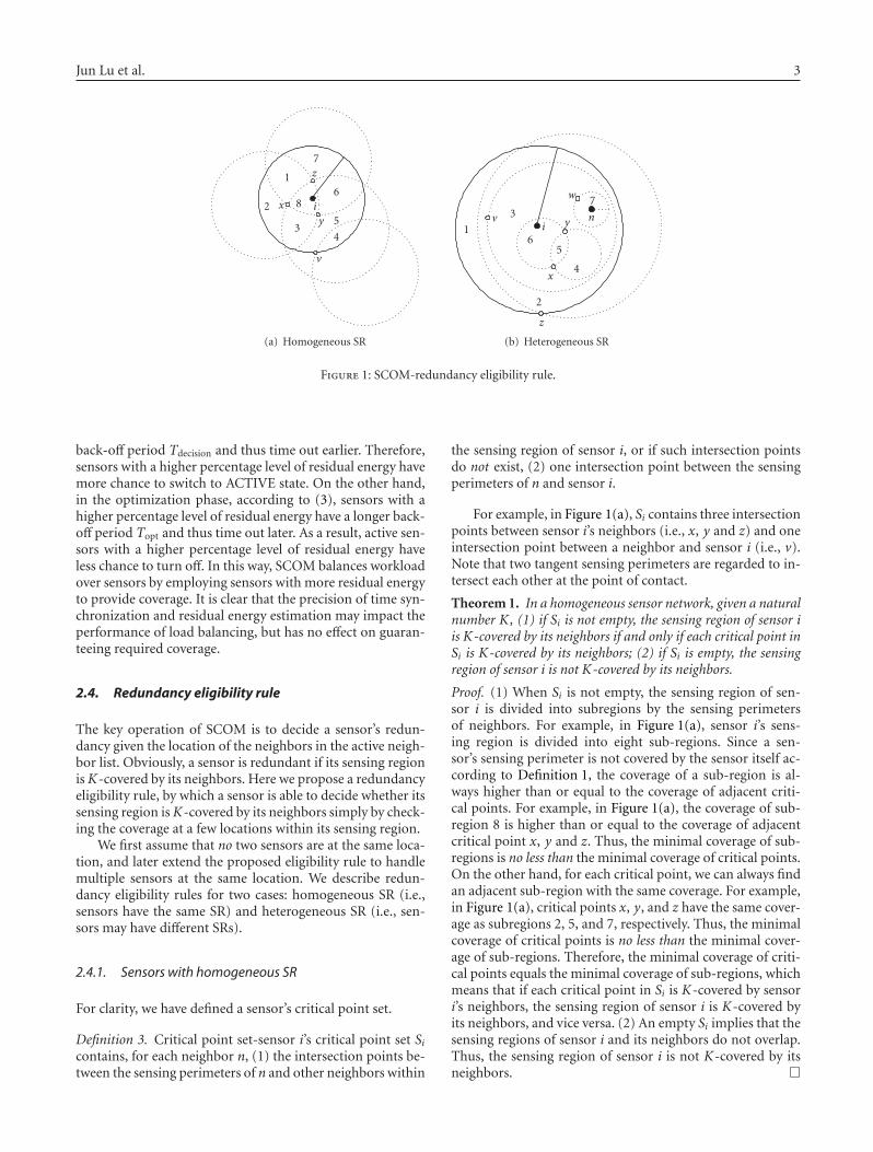
Figure 1: SCOM-redundancy eligibility rule.

back-off period Tdecision and thus time out earlier. Therefore,sensors with a higher percentage level of residual energy havemore chance to switch to ACTIVE state. On the other hand,in the optimization phase, according to (3), sensors with ahigher percentage level of residual energy have a longer back-off period Topt and thus time out later. As a result, active sen-sors with a higher percentage level of residual energy haveless chance to turn off. In this way, SCOM balances workloadover sensors by employing sensors with more residual energyto provide coverage. It is clear that the precision of time syn-chronization and residual energy estimation may impact theperformance of load balancing, but has no effect on guaran-teeing required coverage.

2.4. Redundancy eligibility rule

The key operation of SCOM is to decide a sensor’s redun-dancy given the location of the neighbors in the active neigh-bor list. Obviously, a sensor is redundant if its sensing regionisK-covered by its neighbors. Here we propose a redundancyeligibility rule, by which a sensor is able to decide whether itssensing region isK-covered by its neighbors simply by check-ing the coverage at a few locations within its sensing region.

We first assume that no two sensors are at the same loca-tion, and later extend the proposed eligibility rule to handlemultiple sensors at the same location. We describe redun-dancy eligibility rules for two cases: homogeneous SR (i.e.,sensors have the same SR) and heterogeneous SR (i.e., sen-sors may have different SRs).

2.4.1. Sensors with homogeneous SR

For clarity, we have defined a sensor’s critical point set.

Definition 3. Critical point set-sensor i’s critical point set Sicontains, for each neighbor n, (1) the intersection points be-tween the sensing perimeters of n and other neighbors within

the sensing region of sensor i, or if such intersection pointsdo not exist, (2) one intersection point between the sensingperimeters of n and sensor i.

For example, in Figure 1(a), Si contains three intersectionpoints between sensor i’s neighbors (i.e., x, y and z) and oneintersection point between a neighbor and sensor i (i.e., v).Note that two tangent sensing perimeters are regarded to in-tersect each other at the point of contact.

Theorem 1. In a homogeneous sensor network, given a naturalnumber K , (1) if Si is not empty, the sensing region of sensor iis K-covered by its neighbors if and only if each critical point inSi is K-covered by its neighbors; (2) if Si is empty, the sensingregion of sensor i is not K-covered by its neighbors.

Proof. (1) When Si is not empty, the sensing region of sen-sor i is divided into subregions by the sensing perimetersof neighbors. For example, in Figure 1(a), sensor i’s sens-ing region is divided into eight sub-regions. Since a sen-sor’s sensing perimeter is not covered by the sensor itself ac-cording to Definition 1, the coverage of a sub-region is al-ways higher than or equal to the coverage of adjacent criti-cal points. For example, in Figure 1(a), the coverage of sub-region 8 is higher than or equal to the coverage of adjacentcritical point x, y and z. Thus, the minimal coverage of sub-regions is no less than the minimal coverage of critical points.On the other hand, for each critical point, we can always findan adjacent sub-region with the same coverage. For example,in Figure 1(a), critical points x, y, and z have the same cover-age as subregions 2, 5, and 7, respectively. Thus, the minimalcoverage of critical points is no less than the minimal cover-age of sub-regions. Therefore, the minimal coverage of criti-cal points equals the minimal coverage of sub-regions, whichmeans that if each critical point in Si is K-covered by sensori’s neighbors, the sensing region of sensor i is K-covered byits neighbors, and vice versa. (2) An empty Si implies that thesensing regions of sensor i and its neighbors do not overlap.Thus, the sensing region of sensor i is not K-covered by itsneighbors.


x

i

y

SRi

Figure 2: Theorem 1 cannot be applied for heterogeneous sensors.

2.4.2. Sensors with heterogeneous SR

When sensors have different SRs, Theorem 1 may not hold.For example, in Figure 2, Si contains critical points x and y,both of which are 1-covered by sensor i’s neighbors. How-ever, the sensing region of sensor i is not 1-covered by itsneighbors. To accommodate heterogeneous sensors, we havedefined extended critical point set.

Definition 4. Extended critical point set-sensor i’s extendedcritical point set ESi contains (1) the critical points in crit-ical point set Si, and (2) a sampling point on each sensingperimeter that is within sensor i’s sensing region and doesnot intersect with any other sensing perimeter.

For example, in Figure 1(b), Si contains three criticalpoints, x, y and z. There are two sensing perimeters that arecontained in sensor i’s sensing region and that do not inter-sect with other sensing perimeters. Thus, ESi also contains vand w as the sampling points on the two sensing perimeters.Therefore, ESi contains five critical points, x, y, z, w, and v.

Theorem 2. In a heterogeneous sensor network, given a nat-ural number K , (1) if ESi is not empty, the sensing region ofsensor i is K-covered by its neighbors if and only if each criticalpoint in ESi is K-covered by its neighbors; (2) if ESi is empty,the sensing region of sensor i is K-covered by neighboring sen-sors if and only if a sampling point within the sensing region ofsensor i is K-covered by its neighbors.

Proof. (1) The proof is similar to Theorem 1. We can provethat the minimal coverage of the critical points in ESi is equalto the minimal coverage of the sub-regions, which meansthat if each critical point in ESi is K-covered by sensor i’sneighbors, the sensing region of sensor i is also K-coveredby its neighbors, and vice versa. (2) When sensors have het-erogeneous SR, an empty extended critical point set does notnecessarily mean that the sensing region has no overlap withothers. For example, in Figure 1(b), ESn contains no criticalpoint, but sensor n’s sensing region is contained in the sens-ing regions of its neighbors. In this case, the sensing region ofn is not divided into sub-regions. Thus, sensor n can decidewhether its sensing region is K-covered by checking the cov-erage of any sampling point within its sensing region.

x

v

i

y z

u

Figure 3: Critical point set versus the existing algorithms.

For the description above, we assume that no two sensorsare at the same location. The redundancy eligibility rules de-scribed in Theorems 1 and 2 can be easily extended to accom-modate the special case of multiple sensors at the same loca-tion. For sensors with homogeneous SR, if Si is not empty,the coverage of the critical points on sensor i’s sensing perime-ter (e.g., v in Figure 1(a)) is increased by the number of sen-sors at the same location as sensor i; if Si is empty, the sens-ing area of sensor i is covered by the number of sensors at thesame location as sensor i. In the case of heterogeneous SR, ifESi is not empty, the coverage of the critical points on sensori’s sensing perimeter (e.g., z in Figure 1(b)) is increased by thenumber of sensors at the same location and with the same SRas sensor i; in the case of an empty ESi, we can still decide theredundancy of sensor i by checking a sampling point withinits sensing region.

We note that a similar idea was proposed in Hall (1998)[15, page 56] to study the problem of covering a sphere withcircular caps and later developed by [16, 17] for K-coveragemaintenance in sensor networks. In their algorithms, how-ever, the set of points to be checked by each sensor includesall the intersection points between the sensing perimetersof any two neighbors or between a neighbor and the sen-sor itself. Thus, their algorithms are required to check morepoints, and as a result, incur more computation overhead.For example, in Figure 3, critical point set Si only containspoint x, while the existing algorithms are required to com-pute coverage at all the intersection points, x, y, z, u, andv. Furthermore, the algorithms proposed in [15–17], assumehomogeneous caps or sensors and cannot be applied to het-erogeneous sensors.

3. SCHEME ANALYSIS

In this section, we analyze and compare the scalability ofSCOM with the existing schemes proposed in [4, 6].

In the scheme proposed in [4] (hereinafter referred to asthe sponsored sector (SS) scheme), every sensor calculates itseligibility to turn off. A sensor is eligible to turn off if its sens-ing region is contained by the union of the sponsored sectorsoffered by its active neighbors within SR. A back-off mecha-nism is used to avoid blind points caused by simultaneousdecisions of multiple sensors. After the back-off period, asensor eligible to turn off broadcasts a TURNOFF beacon

Jun Lu et al. 5

to the neighbors within SR. Upon receiving the TURNOFFbeacon, every neighbor removes the sensor from the neigh-bor list so that the sensor will not be counted to decide theeligibility of other sensors.

In the scheme proposed in [6] (referred to as the basic dif-ferentiated surveillance (DS)), each sensor randomly gener-ates a time-reference point and broadcasts it to the neighborswithin twice SR. The target region is covered with a virtualsquare grid. A sensor decides the working schedule for eachgrid point within the SR based on its own time-referencepoint and the time-reference points of the neighbors cov-ering the grid point. The final schedule of the sensor is theunion of the working schedules for all the grid points. The fi-nal schedule can be optimized through exchanging scheduleinformation among neighboring sensors (referred to as 2ndpass differentiated surveillance (DS)).

Let us investigate a sensor network composed of N ho-mogeneous sensors with sensing range R uniformly deployedin a square area of �× � (R� �). For each scheme, we exam-ine the growth of communication overhead (i.e., the num-ber of transmitted and received beacons) and computationalcomplexity (i.e., space and time complexity) as N →∞.

3.1. SCOM

Assume that there are M sensors turning on in the decisionphase and N ′(N ′ � M) active sensors in the final network.

Theorem 3. Given a limited required degree of coverageK , onehas

limN→∞

E(M) = O(1), (4)

where E(M) is the expected number of sensors that turn on inthe decision phase of SCOM.

Proof. Without losing generality, we investigate a sensor net-work within a unit square area (i.e., � is set to 1).

Let us first consider the independent turning on process,in which N sensors are uniformly deployed in BOOTSTRAPstate initially and then randomly and independently turn onone by one until 1-coverage is fulfilled. It is clear that thelocation of the sensors turning on follows a stationary two-dimensional Poisson point process. Denote the density of thePoisson point process and the vacancy (i.e., the region not 1-covered) as λ and Vλ, respectively. It has been shown in Hall(1988) [15, Theorem 3.11, page 180] that

0.05ζλ < P(Vλ > 0

)< 3ζλ, (5)

where ζλ = min{1, (1 + πR2λ2)e−πR2λ}.Obviously, the (n+ 1)th sensor turns on only when the n

sensors that are already on cannot cover the area. Thus, theprobability of requiring more than n active sensors can becalculated as the probability of vacancy larger than 0 with nactive sensors, or

P(M > n) = P(Vn/�2 > 0

) = P(Vn > 0

). (6)

Therefore, we have

E(M) =∞∑

n=1

n · P(M = n)

<∞∑

n=1

n · P(M > n− 1)

=∞∑

n=1

n · P(Vn−1 > 0)

<∞∑

n=1

n · 3ζn−1

<∞∑

n=1

n · 3(1 + πR2(n− 1)2)e−πR

2(n−1).

(7)

We can easily prove the convergence of the series in (7)with the ratio test

limn→∞

3(n+1)(1+πR2n2

)e−πR2n

3n(1+πR2(n−1)2

)e−πR2(n−1)

=e−πR2<1. (8)

The convergence of the series indicates that E(M) to pro-vide 1-coverage is bounded by an upper limit, or O(1) asN →∞.

In [18] (the proof of Theorem 1), Zhang and Huo pre-sented an upper bound of the probability that a region is notK-covered. With the upper bound, we can prove that the ex-pected number of sensors to provide K-coverage is also up-per bounded by a limit, or O(1) as N →∞. Since the proof isessentially the same as the 1-coverage case, we have omittedit here.

We have shown that E(M) of the independent turning onprocess is O(1) as N → ∞. The difference between the de-cision phase of SCOM and the independent turning on pro-cess is that, in the decision phase of SCOM, a sensor turns ononly when it is not redundant (instead of turning on inde-pendently). It is clear that the decision phase of SCOM yieldsfewer active sensors than the independent turning on pro-cess. Therefore, E(M) of the decision phase of SCOM is alsoO(1) as N →∞.

3.1.1. Communication overhead

(a) Number of transmitted beacons

In SCOM, sensors transmit TURNON beacons andTURNOFF beacons in the decision phase and optimizationphase, respectively. It is clear that sensors transmit MTURNON beacons in the decision phase and (M − N ′)TURNOFF beacons in the optimization phase (note that N ′

is the number of active sensors after the optimization phase,which is no larger than M). The total number of transmittedbeacons is (2M −N ′), or O(1) as N →∞.

(b) Number of received beacons

In the decision phase, only the sensors in BOOTSTRAP orACTIVE state need to receive TURNON beacons. The av-erage number of neighbors in BOOTSTRAP or ACTIVE


state of each sensor is upper bounded by Nπ(2R)2/�2 (inSCOM neighbor sensors are within the range of 2R). Sincethere are in total M TURNON beacons transmitted, the totalnumber of TURNON beacons received is upper bounded byMNπ(2R)2/�2. In the optimization phase, only the sensors inACTIVE state accept TURNOFF beacons. Since the averagenumber of neighbors in ACTIVE state of each sensor is upperbounded by Mπ(2R)2/�2 and there are (M −N ′) TURNOFFbeacons transmitted, the total number of TURNOFF beaconsreceived is upper bounded by Mπ(2R)2(M −N ′)/�2. The to-tal number of TURNON and TURNOFF beacons received isupper bounded by MNπ(2R)2/�2 +Mπ(2R)2(M−N ′)/�2, orO(N) as N →∞.

3.1.2. Computational complexity

(a) Time complexity

In the decision phase, each sensor applies the redundancy eli-gibility rule to decide redundancy. The critical point set com-prises the intersection points between the sensing perime-ters of the sensor and its active neighbors. The average num-ber of active neighbors of each sensor is upper bounded byMπ(2R)2/�2. Thus, the number of critical points is upperbounded by 2 · (Mπ(2R)2/�2)(1 + Mπ(2R)2/�2). For eachcritical point, a sensor needs to check for each active neigh-bor whether the critical point is covered. Thus, the num-ber of basic computation steps to decide the redundancy is2 · (Mπ(2R)2/�2)2(1 + Mπ(2R)2/�2), or O(1) as N → ∞. Inthe optimization phase, each active sensor checks its redun-dancy once, the number of basic computation steps of whichis also O(1). Thus, the time complexity is O(1) as N →∞.

(b) Space complexity

The memory size required for each sensor to execute SCOMis mainly composed of (1) Mπ(2R)2/�2 entries for neighborsin ACTIVE state and (2) 2 · (Mπ(2R)2/�2)(1 +Mπ(2R)2/�2)entries for critical points. Thus, the space complexity is O(1)as N →∞.

3.2. Sponsored sector scheme

Denote the number of active sensors in the resulting networkof SS as N ′. Similarly, we can derive that E(N ′) of SS is O(1)when N →∞.



Each sensor to turn off sends a TURNOFF beacon to informits neighbors. Obviously, the total number of TURNOFFbeacons transmitted is (N −N ′), or O(N) as N →∞.


Only sensors that have not made their decisions need to re-ceive TURNOFF beacons. In the best case, all the N ′ ac-tive sensors make decisions before the other sensors, and

thus no beacon is received by these N ′ sensors. Therefore,TURNOFF beacons are only exchanged among the (N −N ′)sensors. For the ith sensor to turn off, the average num-ber of received TURNOFF beacons is (i − 1)πR2/�2 (in SSneighbor sensors are within the range of R). Thus, the totalnumber of TURNOFF beacons received by all the sensors is∑N−N ′

i=1 ((i− 1)πR2/�2), or O(N2) as N →∞.


(a) Time complexity

In SS, each sensor checks all the active neighbors to de-cide its redundancy. Thus, the computational complexity isin the order of the number of active neighbors. A lowerbound of the computational complexity can be derived bymerely counting the computation overhead of the (N − N ′)inactive sensors in the resulting network. For the ith sen-sor to turn off, the average number of active neighbors is(N − i+ 1)(πR2/�2). Thus, the total computational complex-ity of all the sensors is O(

∑N−N ′i=1 ((N − i + 1)πR2/�2)), or

O(N2). Thus, the average time complexity per sensor is O(N)as N →∞.


The memory size required for each sensor is mainly com-posed ofNπR2/�2 entries on average to store neighbor states.Thus, the space complexity is O(N).

3.3. Basic differentiated surveillance


It is noted in [6] that the time-reference point beacons can becombined with the beacons to exchange coordinates amongneighbors. Thus, there is no extra communication overheadin Basic DS.


(a) Time complexity

As described in [6], there are averagely πR2/d2 grid pointswithin a sensor’s sensing region, where d is the unit gridsize. Each sensor decides the schedule for each grid point ac-cording to neighbors’ time reference points. Given NπR2/�2

neighbors on average covering the same grid point, it takes(NπR2/�2) log(NπR2/�2) basic computation steps to sorttime-reference points and another constant time C to decidethe sensor’s schedule for the grid point. Finally, the sched-ules for all the grid points are combined to generate the in-tegrated schedule for the sensor, which costs 2πR2/d2 basiccomputation steps. Thus, the overall computational com-plexity is (πR2/d2)((NπR2/�2) log(NπR2/�2) +C) + 2πR2/d2,or O(N logN) as N →∞.

Jun Lu et al. 7


As described in [6], the memory size required for each sen-sor is mainly composed of (1)Nπ(2R)2/�2 entries on averagefor a neighbor table, (2) NπR2/�2 memory units on averagefor sorting time reference points and (3) 2πR2/d2 memoryunits for schedules of grid points. The total space complexityis O(N).

3.4. 2nd pass differentiated surveillance



In 2nd pass DS, each sensor sends two beacons to informits original integrated schedule and optimized schedule toneighbors. Thus, the total number of beacons transmitted isO(N).


First, each sensor receives the beacons for original integratedschedules from its neighbors. The total number of receivedbeacons is N · (Nπ(2R)2/�2), or O(N2). Second, only sensorsthat have not optimized need to receive the beacons for opti-mized schedules. For the ith sensor to optimize, the averagenumber of the received beacons is (i−1)π(2R)2/�2. Thus, thetotal number of received beacons for the optimized sched-ule is

∑Ni=1((i− 1)π(2R)2/�2), or O(N2). Therefore, the total

number of received beacons is O(N2).


(a) Time complexity

In 2nd pass DS, each sensor carries out the basic DS algo-rithm and optimizes its schedule according to the schedulesof its neighbors, both of which can be done in O(N logN).Thus, the time complexity is O(N logN).


The memory capacity required for each sensor is mainlycomposed of (1) Nπ(2R)2/�2 entries on average for a neigh-bor table, (2) NπR2/�2 memory units on average for sort-ing time reference points on average, (3) 2πR2/d2 memoryunits on average for schedules for all the grid points and(4) Nπ(2R)2/�2 entries on average for integrated schedulesof neighboring sensors. Thus, the space complexity is O(N).

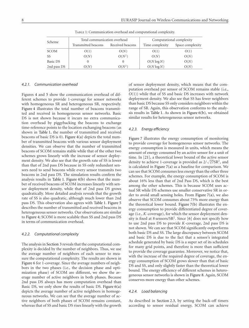
Table 1 summarizes the scalability of different coveragemaintenance schemes to sensor deployment density (notethat given a fixed �, N actually represents sensor deploy-ment density) in terms of total communication overhead(i.e., number of transmitted and received beacons) and com-putational complexity (i.e., time and space complexity). Wecan see that SCOM outperforms other schemes except for thecommunication overhead of basic DS. However, the achieve-ment of Basic DS is at the cost of energy efficiency and adapt-ability to sensor network dynamics such as sensor failures.

An integrated schedule generated by basic DS is a super set ofschedules for many grid points, and therefore may be morethan sufficient to provide the coverage guarantee. Moreover,when executed in multiple rounds, basic DS is not able torestore coverage from sensor failure because sensors are un-aware of the failure of neighboring sensors. Although it ispossible to use heartbeat signals to check the state of neigh-bors as described in [6], the communication overhead totransmit and receive heartbeat signals isO(N) andO(N2), re-spectively. In contrast, at the beginning of each round, sinceonly working sensors turn on and transmit TURNON bea-cons, SCOM can easily restore the coverage by substitutingfailed sensors with working ones.

Note that we assumed sensors with homogeneous SR inthe above analysis. The analysis results are also valid for het-erogeneous sensor networks as long as the SR is within a lim-ited range.

From the above analysis, we know that SCOM is scal-able because it only turns on necessary sensors in the deci-sion phase. We have shown that, given the required degreeof coverage, the number of sensors turning on in the deci-sion phase is a limited value as sensor deployment densityapproaches infinity. Since each sensor only communicates toits active neighbors and only considers the active neighborsto make its decision, the communication and computationoverhead per sensor remains limited with the increase of sen-sor deployment density. A similar technique is adopted by[17, 19, 20], but they do not provide specific analysis andevaluation of scalability of their schemes.

In summary, communication overhead and computa-tional complexity per sensor are limited as the sensor deploy-ment density approaches infinity, which makes SCOM favor-able for dense sensor networks composed of simple sensorsequipped with a slow processor and small storage.

4. SIMULATION STUDY

In this section, we compare the performance of SCOM withSS, DS, and 2nd pass DS schemes through simulations.

4.1. Simulation setup

The simulations are carried out over a square region of100 m× 100 m with wrap around in both dimensions. Thus,the results are representative of an infinite system, and there-fore apply to typical large-scale sensor networks. Sensors areuniformly deployed in the square region.

In SCOM, α and χ of (2) and (3) are set to 10.0 and 1.0,respectively. We simulated both homogeneous and hetero-geneous sensor networks. For homogeneous networks, SR isfixed at 10 m. For heterogeneous networks, a sensor’s SR isuniformly chosen from three possible values: 5 m, 10 m, and15 m.

4.2. Simulation results

The simulation results are shown for communication over-head, computational complexity, energy efficiency, and loadbalancing.


Table 1: Communication overhead and computational complexity.

SchemeTotal communication overhead Computational complexity

Transmitted beacons Received beacons Time complexity Space complexity

SCOM O(1) O(N) O(1) O(1)

SS O(N) O(N2) O(N) O(N)

Basic DS 0 0 O(N logN) O(N)

2nd pass DS O(N) O(N2) O(N logN) O(N)


Figures 4 and 5 show the communication overhead of dif-ferent schemes to provide 1-coverage for sensor networkswith homogeneous SR and heterogeneous SR, respectively.Figure 4 illustrates the total number of beacons transmit-ted and received in homogeneous sensor networks. BasicDS is not shown because it incurs no extra communica-tion overhead by piggybacking the beacons to exchangetime-reference points to the location exchanging beacons (asshown in Table 1, the number of transmitted and receivedbeacons of basic DS is 0). Figure 4(a) depicts the total num-ber of transmitted beacons with various sensor deploymentdensities. We can observe that the number of transmittedbeacons of SCOM remains stable while that of the other twoschemes grows linearly with the increase of sensor deploy-ment density. We also see that the growth rate of SS is lowerthan that of 2nd pass DS because in SS only redundant sen-sors need to send beacons while every sensor transmits twobeacons in 2nd pass DS. The simulation results confirm theanalysis results in Table 1. Figure 4(b) shows that the num-ber of received beacons of SCOM increases linearly with sen-sor deployment density, while that of 2nd pass DS growsquadratically. More detailed analysis reveals that the growthrate of SS is also quadratic, although much lower than 2ndpass DS. This observation also agrees with Table 1. Figure 5describes the number of transmitted and received beacons inheterogeneous sensor networks. Our observations are similarto Figure 4; SCOM is more scalable than SS and 2nd pass DSin terms of communication overhead.


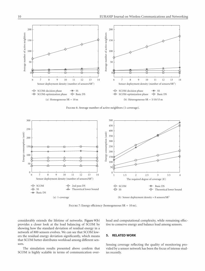
The analysis in Section 3 reveals that the computational com-plexity is decided by the number of neighbors. Thus, we usethe average number of neighbors of each sensor to mea-sure the computational complexity. The results are shown inFigure 6 for 1-coverage. Since the average numbers of neigh-bors in the two phases (i.e., the decision phase and opti-mization phase) of SCOM are different, we show the av-erage number of active neighbors in both phases. Because2nd pass DS always has more computation overhead thanBasic DS, we only show the results of basic DS. Figure 6(a)depicts the average number of active neighbors in homoge-neous networks. We can see that the average number of ac-tive neighbors of both phases of SCOM remains constant,whereas that of SS and basic DS rises linearly with the growth

of sensor deployment density, which means that the com-putation overhead per sensor of SCOM remains stable (i.e.,O(1)) while that of SS and basic DS increases with networkdeployment density. We also see that SS has fewer neighborsthan basic DS because SS only considers neighbors within therange of SR. Again, this observation conforms to the analy-sis results in Table 1. As shown in Figure 6(b), we obtainedsimilar results for heterogeneous sensor networks.

4.2.3. Energy efficiency

Figure 7 illustrates the energy consumption of monitoringto provide coverage for homogeneous sensor networks. Theenergy consumption is measured in units, which means theamount of energy consumed by an active sensor for a unit oftime. In [21], a theoretical lower bound of the active sensordensity to achieve 1-coverage is provided as 2/

√27SR2, and

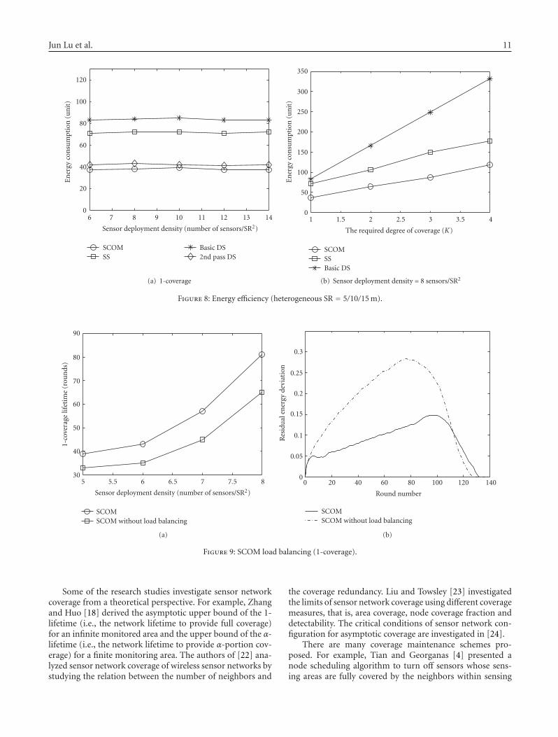
is calculated in Figure 7(a) as a baseline for comparison. Wecan see that SCOM consumes less energy than the other threeschemes. For example, the energy consumption of SCOM isabout 16% less than that of 2nd Pass DS, which is the bestamong the other schemes. This is because SCOM uses ac-tual SR while DS schemes use smaller conservative SR in or-der to avoid small sensing holes. From Figure 7(a), we alsoobserve that SCOM consumes about 75% more energy thanthe theoretical lower bound. Figure 7(b) illustrates the en-ergy consumption to provide differentiated degree of cover-age (i.e., K-coverage), for which the sensor deployment den-sity is fixed at 8 sensors/SR2. Since [6] does not specify howto use 2nd pass DS to provide K-coverage, 2nd pass DS isnot shown. We can see that SCOM significantly outperformsboth basic DS and SS. The large discrepancy between SCOMand basic DS is due to the fact that a sensor’s integratedschedule generated by basic DS is a super set of its schedulesfor many grid points, and therefore is more than sufficientto provide the coverage guarantee. Moreover, we notice that,with the increase of the required degree of coverage, the en-ergy consumption of SCOM grows slower than that of basicDS and SS, and only slightly faster than the theoretical lowerbound. The energy efficiency of different schemes in hetero-geneous sensor networks is shown in Figure 8. Again, SCOMconserves more energy than other schemes.

4.2.4. Load balancing

As described in Section 2.3, by setting the back-off timersaccording to sensor residual energy, SCOM can achieve

Jun Lu et al. 9

500

0

1000

1500

2000

2500

3000

3500

Tota

lnu

mbe

rof

tran

smit

ted

beac

ons

6 7 8 9 10 11 12 13 14

Sensor deployment density (number of sensors/SR2)

SCOMSS2nd pass DS

(a) Beacons transmitted

0.5

0

1

1.5

2

2.5

3

3.5×105

Tota

lnu

mbe

rof

rece

ived

beac

ons

6 7 8 9 10 11 12 13 14


SCOMSS2nd pass DS

(b) Beacons received

Figure 4: Communication overhead (1-coverage, homogeneous SR = 10 m).

500

0

1000

1500

2000

2500

3000

3500

Tota

lnu

mbe

rof

tran

smit

ted

beac

ons

6 7 8 9 10 11 12 13 14


SCOMSS2nd pass DS

(a) Beacons transmitted

0.5

0

1

1.5

2

2.5

3

3.5

4×105

Tota

lnu

mbe

rof

rece

ived

beac

ons

6 7 8 9 10 11 12 13 14


SCOMSS2nd pass DS

(b) Beacons received

Figure 5: Communication overhead (1-coverage, heterogeneous SR = 5/10/15 m).

load balancing by employing sensors with more percent-age of residual energy to provide network coverage. Herewe compare SCOM with a modified version of SCOM (re-ferred to as SCOM without load balancing). In SCOM with-out load balancing, instead of setting timers according to theamount of residual energy using (2) and (3), sensors simply

adopt random back-off timers. In the simulations, each sen-sor starts with 100% energy and the energy consumption rateis fixed at 10% per round. Figure 9(a) depicts the networklifetime of maintaining 1-coverage, which is measured as thetime from the beginning of the deployment until the networkloses 1-coverage of the target region. We can see that SCOM


0

50

100

150

200

Ave

rage

nu

mbe

rof

acti

ven

eigh

bors

6 7 8 9 10 11 12 13 14


SCOM-decision phaseSCOM-optimization phase

SSBasic DS

(a) Homogeneous SR = 10 m

0

50

100

150

200

Ave

rage

nu

mbe

rof

acti

ven

eigh

bors

6 7 8 9 10 11 12 13 14


SCOM-decision phaseSCOM-optimization phase

SSBasic DS

(b) Heterogeneous SR = 5/10/15 m

Figure 6: Average number of active neighbors (1-coverage).

50

0

100

150

200

250

300

En

ergy

con

sum

ptio

n(u

nit

)

6 7 8 9 10 11 12 13 14


SCOMSSBasic DS

2nd pass DSTheoretical lower bound

(a) 1-coverage

0

50

100

150

200

250

300

350

400

450

500

En

ergy

con

sum

ptio

n(u

nit

)

1 1.5 2 2.5 3 3.5 4

The required degree of coverage (K)

SCOMSS

Basic DSTheoretical lower bound

(b) Sensor deployment density = 8 sensors/SR2

Figure 7: Energy efficiency (homogeneous SR = 10 m).

considerably extends the lifetime of networks. Figure 9(b)provides a closer look at the load balancing of SCOM byshowing how the standard deviation of residual energy in anetwork of 800 sensors evolves. We can see that SCOM low-ers the residual energy deviation significantly, which meansthat SCOM better distributes workload among different sen-sors.

The simulation results presented above confirm thatSCOM is highly scalable in terms of communication over-

head and computational complexity, while remaining effec-tive to conserve energy and balance load among sensors.

5. RELATED WORK

Sensing coverage reflecting the quality of monitoring pro-vided by a sensor network has been the focus of intense stud-ies recently.

Jun Lu et al. 11

20

0

40

60

80

100

120

En

ergy

con

sum

ptio

n(u

nit

)

6 7 8 9 10 11 12 13 14


SCOMSS

Basic DS2nd pass DS

(a) 1-coverage

0

50

100

150

200

250

300

350

En

ergy

con

sum

ptio

n(u

nit

)

1 1.5 2 2.5 3 3.5 4

The required degree of coverage (K)

SCOMSSBasic DS

(b) Sensor deployment density = 8 sensors/SR2

Figure 8: Energy efficiency (heterogeneous SR = 5/10/15 m).

30

40

50

60

70

80

90

1-co

vera

gelif

etim

e(r

oun

ds)

5 5.5 6 6.5 7 7.5 8


SCOMSCOM without load balancing

(a)

0

0.05

0.1

0.15

0.2

0.25

0.3

Res

idu

alen

ergy

devi

atio

n

0 20 40 60 80 100 120 140

Round number

SCOMSCOM without load balancing

(b)

Figure 9: SCOM load balancing (1-coverage).

Some of the research studies investigate sensor networkcoverage from a theoretical perspective. For example, Zhangand Huo [18] derived the asymptotic upper bound of the 1-lifetime (i.e., the network lifetime to provide full coverage)for an infinite monitored area and the upper bound of the α-lifetime (i.e., the network lifetime to provide α-portion cov-erage) for a finite monitoring area. The authors of [22] ana-lyzed sensor network coverage of wireless sensor networks bystudying the relation between the number of neighbors and

the coverage redundancy. Liu and Towsley [23] investigatedthe limits of sensor network coverage using different coveragemeasures, that is, area coverage, node coverage fraction anddetectability. The critical conditions of sensor network con-figuration for asymptotic coverage are investigated in [24].

There are many coverage maintenance schemes pro-posed. For example, Tian and Georganas [4] presented anode scheduling algorithm to turn off sensors whose sens-ing areas are fully covered by the neighbors within sensing


range. Randomized as well as coordinated sleep algorithmswere proposed in [25] to maintain network coverage usinglow duty-cycle sensors. The randomized algorithm enableseach sensor to independently sleep under a certain proba-bility, while the coordinated sleep algorithm allows a sen-sor to enter sleep state if its sensing area is fully containedby the union set of its neighbors. An algorithm was pro-posed in [5] to decide the coverage of a target area by merelychecking the coverage state of sensing perimeters. Yan etal. [6] proposed an adaptable energy-efficient sensing cov-erage protocol, in which each sensor broadcasts a randomtime-reference point, and decides its duty schedule based onneighbors’ time-reference points. Co-Grid proposed in [14]schedules sensors by adopting a distributed detection modelbased on data fusion. Abrams et al. studied a variant of theNP-hard SET K-COVER problem in [26], partitioning thesensors into K covers such that as many areas are monitoredas frequently as possible. Xing et al. [16] studied the relation-ship between coverage and connectivity, and proposed a cov-erage maintenance scheme, coverage configuration protocol(CCP), which, when integrated with an existing connectivitymaintenance scheme, is able to provide both coverage andconnectivity guarantees. In [27], Kumar et al. proposed al-gorithms to decide quickly whether a deployed region is K-barrier covered. Two notions of probabilistic barrier cover-age, the weak and strong barrier coverage, are introduced andstudied. Cardei et al. [28] proposed an efficient scheme tocover a set of targets with known locations in a randomly anddensely deployed sensor network. The target coverage prob-lem is modeled as the maximal set cover problem and twoheuristics are proposed and evaluated. Zhang and Huo [19]presented a scheme to optimize coverage maintenance whileproviding global connectivity by keeping a minimum num-ber of active sensors to minimize coverage redundancy.

6. CONCLUSION

In this paper, we introduced SCOM that conserves energywhile preserving the required sensing coverage by allowingsensors to autonomously decide their active/inactive states.An important property of SCOM is the high scalability tosensor deployment density in terms of communication over-head and computational complexity, which makes SCOMsuitable for densely deployed sensor networks composed ofsimple sensors. We showed that the scalability of SCOMis better than the earlier works through both theoreticalanalysis and simulation study. Moreover, we demonstratedthrough simulation study that SCOM outperforms severalexisting competitors on energy efficiency and effectively bal-ances workload among sensors.

ACKNOWLEDGMENTS

This research is supported by the NSF through GrantsANI-0083074, ANI-9903427, and ANI-0508506, by DARPAthrough Grant MDA972-99-1-0007, by AFOSR throughGrant MURI F49620-00-1- 0330, and by grants from the Cal-ifornia MICRO and CoRe programs, Hitachi, Hitachi Amer-

ica, Hitachi CRL, Hitachi SDL, DENSO IT Laboratory, NICT(National Institute of Communication Technology, Japan),Nippon Telegraph and Telephone (NTT), NTT Docomo, NSSolutions Corporation, Fujitsu and Novell.

REFERENCES

[1] Crossbow Technology Inc., MICA2 Data Sheet, http://www.xbow.com/products/Product pdf files/Wireless pdf/MICA2 Datasheet.pdf.

[2] K. S. J. Pister, J. M. Kahn, and B. E. Boser, “Smart Dust:Wireless Networks of Millimeter-Scale Sensor Nodes,” High-light Article in 1999 Electronics Research Laboratory ResearchSummary, 1999.

[3] B. Warneke, M. Last, B. Liebowitz, and K. S. J. Pister, “Smartdust: communicating with a cubic-millimeter computer,”Computer, vol. 34, no. 1, pp. 44–51, 2001.

[4] D. Tian and N. D. Georganas, “A coverage-preserving nodescheduling scheme for large wireless sensor networks,” in Pro-ceedings of the 1st ACM International Workshop on WirelessSensor Networks and Applications (WSNA ’02), pp. 32–41, At-lanta, Ga, USA, September 2002.

[5] C.-F. Huang and Y.-C. Tseng, “The coverage problem in a wire-less sensor network,” in Proceedings of the 2nd ACM Interna-tional Workshop on Wireless Sensor Networks and Applications(WSNA ’03), pp. 115–121, San Diego, Calif, USA, September2003.

[6] T. Yan, T. He, and J. A. Stankovic, “Differentiated surveil-lance for sensor networks,” in Proceedings of the 1st Interna-tional Conference on Embedded Networked Sensor Systems (Sen-Sys ’03), pp. 51–62, Los Angeles, Calif, USA, November 2003.

[7] J. Albowicz, A. Chen, and L. Zhang, “Recursive position es-timation in sensor networks,” in Proceedings of InternationalConference on Network Protocols (ICNP ’01), pp. 35–41, River-side, Calif, USA, November 2001.

[8] N. Bulusu, J. Heidemann, and D. Estrin, “GPS-less low-costoutdoor localization for very small devices,” IEEE PersonalCommunications, vol. 7, no. 5, pp. 28–34, 2000.

[9] P. Bahl and V. N. Padmanabhan, “RADAR: an in-building RF-based user location and tracking system,” in Proceedings of the19th Annual Joint Conference of the IEEE Computer and Com-munications Societies (INFOCOM ’00), vol. 2, pp. 775–784, TelAviv, Israel, March 2000.

[10] N. B. Priyantha, A. Chakraborty, and H. Balakrishnan, “TheCricket location-support system,” in Proceedings of the 6th An-nual International Conference on Mobile Computing and Net-working (MOBICOM ’00), pp. 32–43, Boston, Mass, USA,August 2000.

[11] H. Dai and R. Han, “TSync: a lightweight bidirectional timesynchronization service for wireless sensor networks,” ACMSIGMOBILE Mobile Computing and Communications Review,vol. 8, no. 1, pp. 125–139, 2004.

[12] J. Elson, L. Girod, and D. Estrin, “Fine-grained network timesynchronization using reference broadcasts,” in Proceedings ofthe 5th Symposium on Operating System Design and Implemen-tation (OSDI ’02), pp. 147–163, Boston, Mass, USA, December2002.

[13] Crossbow Technology Inc., MTS/MDA Sensor and Data Ac-quisition Boards Users Manual, Crossbow Technology Inc, SanJose, Calif, USA, 2003.

[14] G. Xing, C. Lu, R. Pless, and J. A. O’Sullivan, “Co-Grid: an ef-ficient coverage maintenance protocol for distributed sensornetworks,” in Proceedings of the 3rd International Symposium

http://www.xbow.com/products/Product_pdf_files/Wireless_pdf/MICA2_Datasheet.pdf



Jun Lu et al. 13

on Information Processing in Sensor Networks (IPSN ’04),pp. 414–423, Berkeley, Calif, USA, April 2004.

[15] P. Hall, Introduction to the Theory of Coverage Processes, JohnWiley & Sons, New York, NY, USA, 1988.

[16] G. Xing, X. Wang, Y. Zhang, C. Lu, R. Pless, and C. Gill, “In-tegrated coverage and connectivity configuration for energyconservation in sensor networks,” ACM Transactions on Sen-sor Networks, vol. 1, no. 1, pp. 36–72, 2005.

[17] A. Gallais, J. Carle, D. Simplot-Ryl, and I. Stojmenovic, “Local-ized sensor area coverage with low communication overhead,”in Proceedings of the 4th Annual IEEE International Conferenceon Pervasive Computing and Communications (PerCom ’06),pp. 328–337, Pisa, Italy, March 2006.

[18] H. Zhang and J. C. Hou, “On deriving the upper bound of α-lifetime for large sensor networks,” in Proceedings of the 5thACM International Symposium on Mobile Ad Hoc Network-ing and Computing (MobiHoc ’04), pp. 121–132, Tokyo, Japan,May 2004.

[19] H. Zhang and J. C. Huo, “Maintaining sensing coverage andconnectivity in large sensor networks,” Ad Hoc & Sensor Wire-less Networks, vol. 1, no. 1-2, pp. 89–123, 2005.

[20] J. Lu and T. Suda, “Coverage-aware self-coordination in sen-sor networks,” Tech. Rep. 04-19, School of Information andComputer Sciences, UC Irvine, Irvine, Calif, USA, 2004.

[21] F. Ye, G. Zhong, S. Lu, and L. Zhang, “Energy efficient robustsensing coverage in large sensor networks,” Tech. Rep., UC LosAngeles, Los Angeles, Calif, USA, 2002.

[22] Y. Gao, K. Wu, and F. Li, “Analysis on the redundancy of wire-less sensor networks,” in Proceedings of the 2nd ACM Interna-tional Workshop on Wireless Sensor Networks and Applications(WSNA ’03), pp. 108–114, San Diego, Calif, USA, September2003.

[23] B. Liu and D. Towsley, “A study of the coverage of large-scale sensor networks,” in Proceedings of IEEE InternationalConference on Mobile Ad-Hoc and Sensor Systems (MASS ’04),pp. 475–483, Fort Lauderdale, Fla, USA, October 2004.

[24] S. Kumar, T. H. Lai, and J. Balogh, “On K-coverage in a mostlysleeping sensor network,” in Proceedings of the 10th AnnualInternational Conference on Mobile Computing and Network-ing (MOBICOM ’04), pp. 144–158, Philadelphia, Pa, USA,September-October 2004.

[25] C.-F. Hsin and M. Liu, “Network coverage using low duty-cycled sensors: random & coordinated sleep algorithms,” inProceedings of the 3rd International Symposium on InformationProcessing in Sensor Networks (IPSN ’04), pp. 433–442, Berke-ley, Calif, USA, April 2004.

[26] Z. Abrams, A. Goel, and S. Plotkin, “Set K-cover algorithmsfor energy efficient monitoring in wireless sensor networks,” inProceedings of the 3rd International Symposium on InformationProcessing in Sensor Networks (IPSN ’04), pp. 424–432, Berke-ley, Calif, USA, April 2004.

[27] S. Kumar, T. H. Lai, and A. Arora, “Barrier coverage withwireless sensors,” in Proceedings of the 11th Annual Inter-national Conference on Mobile Computing and Networking(MOBICOM ’05), pp. 284–298, Cologne, Germany, August-September 2005.

[28] M. Cardei, M. T. Thai, Y. Li, and W. Wu, “Energy-efficient tar-get coverage in wireless sensor networks,” in Proceedings of the24th Annual Joint Conference of the IEEE Computer and Com-munications Societies (INFOCOM ’05), vol. 3, pp. 1976–1984,Miami, Fla, USA, March 2005.

034758

Documents

Transcript of 034758