03 refrigerated gasplant

Refrigerated Gas Plant 1

Refrigerated Gas Plant

1

© 2003 AspenTech. All Rights Reserved.EA1031.31.0503 Refrigerated Gas Plant.pdf

2 Refrigerated Gas Plant

WorkshopIn this simulation, a simplified version of a refrigerated gas plant is going to be modeled. The purpose is to find the LTS (Low Temperature Separator) temperature at which the hydrocarbon dewpoint target is met. The Sales Gas hydrocarbon dewpoint should not exceed -15°C at 6000 kPa. The incoming gas is cooled in two stages—first by exchange with product Sales Gas in a gas-gas exchanger (Gas-Gas) and then in a propane chiller (Chiller), represented here by a Cooler operation. A Balance operation will be used to evaluate the hydrocarbon dewpoint of the product stream at 6000 kPa.

Learning ObjectivesOnce you have completed this section, you will be able to:

• Install and converge heat exchangers. • Understand logical operations (Balances and Adjusts).• Use the Case Study tool to perform case studies on your

simulation.

PrerequisitesBefore beginning this section you need to know how to:

• Create a fluid package.• Add streams.• Add unit operations.

2

Proce

ss Ov

erview


Building the Simulation1. Defining components list and fluid package

2. Adding streams and unit operations

3. Adding logical operation (Balance and Adjust)

Defining the Simulation BasisFor this case, you will be using the Peng Robinson EOS with the following components: N2, H2S, CO2, C1, C2, C3, i-C4, n-C4, i-C5, n-C5, C6, C7+*, and H2O.

1. Create a new case.

2. Import the fluid package, GasPlant, which you saved in Module 1 (Getting Started).

Adding a Feed StreamAdd a new Material stream with the following values:

In this cell... Enter...

Name To Refrig

Temperature 15°C (60°F)

Pressure 6200 kPa (900 psia)

Flow Rate 1440 kgmole/h (3175 lbmole/hr)

Component Mole Fraction

N2 0.0066

H2S 0.0003

CO2 0.0003

C1 0.7575

C2 0.1709

C3 0.0413

i-C4 0.0068

n-C4 0.0101

i-C5 0.0028

n-C5 0.0027

C6 0.0006

If you want to recreate the fluid package, refer to the first module (Getting Started).

4


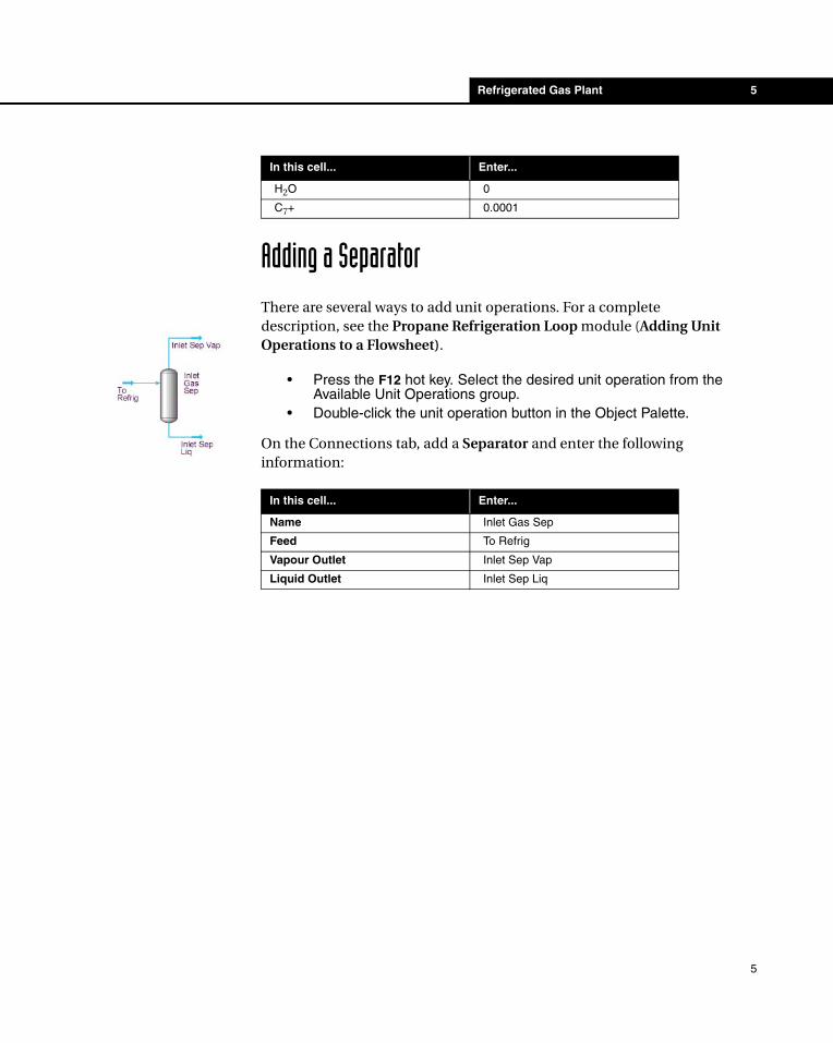
Adding a SeparatorThere are several ways to add unit operations. For a complete description, see the Propane Refrigeration Loop module (Adding Unit Operations to a Flowsheet).

• Press the F12 hot key. Select the desired unit operation from the Available Unit Operations group.

• Double-click the unit operation button in the Object Palette.

On the Connections tab, add a Separator and enter the following information:

H2O 0

C7+ 0.0001


Name Inlet Gas Sep

Feed To Refrig

Vapour Outlet Inlet Sep Vap

Liquid Outlet Inlet Sep Liq


5


Adding a Heat ExchangerThe heat exchanger performs two-sided energy and material balance calculations. The heat exchanger is capable of solving for temperatures, pressures, heat flows (including heat loss and heat leak), material stream flows, and UA.

1. Double-click on the Heat Exchanger button on the Object Palette.

2. On the Connections page, enter the following information:

Figure 1

Heat Exchanger icon

The Tube Side and Shell Side streams can come from different Flowsheets, so you can use the Steam package on one side of the exchanger and PR on the other side.

6


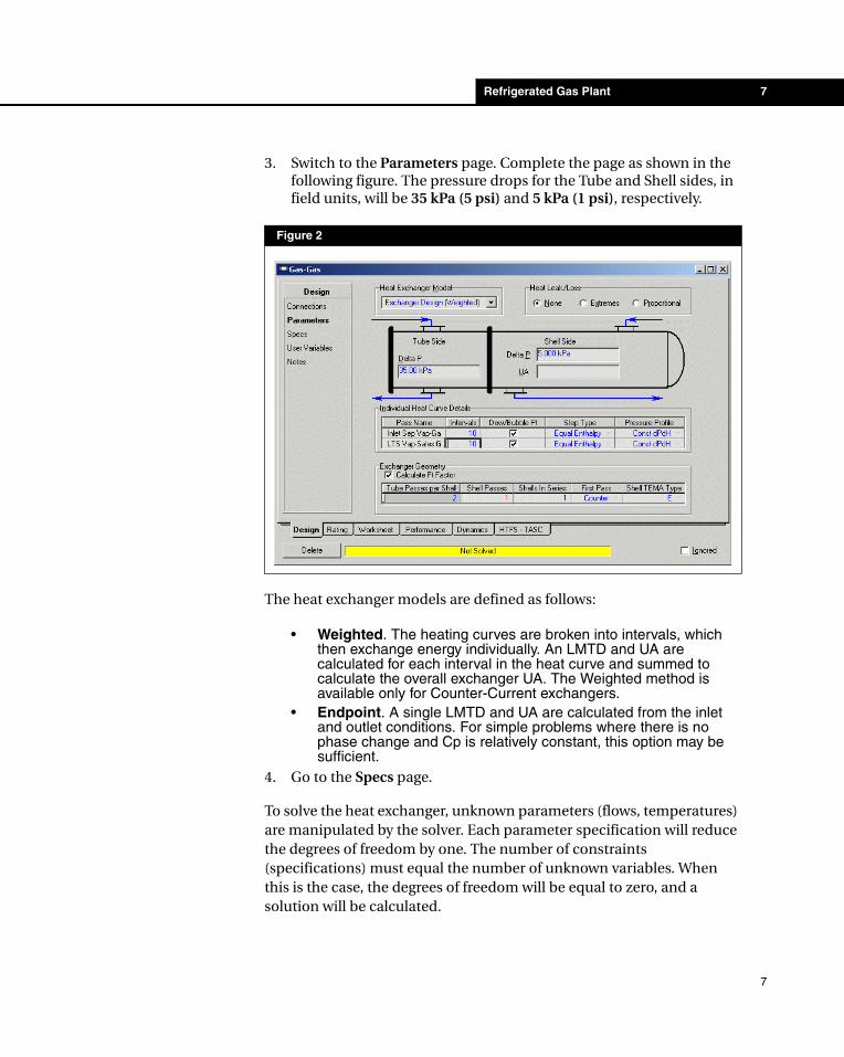
3. Switch to the Parameters page. Complete the page as shown in the following figure. The pressure drops for the Tube and Shell sides, in field units, will be 35 kPa (5 psi) and 5 kPa (1 psi), respectively.

The heat exchanger models are defined as follows:

• Weighted. The heating curves are broken into intervals, which then exchange energy individually. An LMTD and UA are calculated for each interval in the heat curve and summed to calculate the overall exchanger UA. The Weighted method is available only for Counter-Current exchangers.

• Endpoint. A single LMTD and UA are calculated from the inlet and outlet conditions. For simple problems where there is no phase change and Cp is relatively constant, this option may be sufficient.

4. Go to the Specs page.

To solve the heat exchanger, unknown parameters (flows, temperatures) are manipulated by the solver. Each parameter specification will reduce the degrees of freedom by one. The number of constraints (specifications) must equal the number of unknown variables. When this is the case, the degrees of freedom will be equal to zero, and a solution will be calculated.

Figure 2

7


Two specifications are needed for this exchanger:

• Heat Balance = 0. This is a Duty Error specification and is needed to ensure that the heat equation balances. This is a default specification that is always added by HYSYS so you do not need to supply it.

• Min Approach = 5°C. This is the minimum temperature difference between the hot and cold stream.

5. You will first need to deactivate the UA specification. To do this, click on the Active checkbox for the UA specification.

6. To add a specification, click the Add button, the ExchSpec view appears.

7. Provide the following information:

Figure 3


Name Temp Approach

Type Min Approach

Pass Overall

Spec Value 5°C (41°F)

You can have multiple Estimate specifications. The Heat Exchanger will only use the Active specifications for convergence.

8


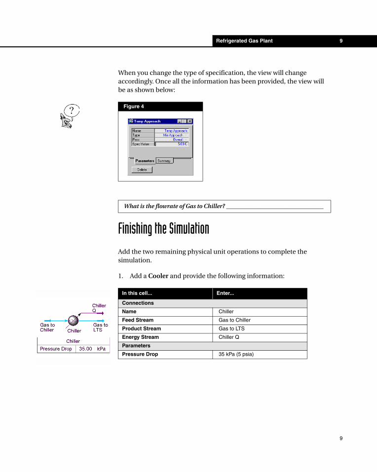
When you change the type of specification, the view will change accordingly. Once all the information has been provided, the view will be as shown below:

Finishing the SimulationAdd the two remaining physical unit operations to complete the simulation.

1. Add a Cooler and provide the following information:

Figure 4

What is the flowrate of Gas to Chiller? _________________________________


Connections

Name Chiller

Feed Stream Gas to Chiller

Product Stream Gas to LTS

Energy Stream Chiller Q

Parameters

Pressure Drop 35 kPa (5 psia)

9


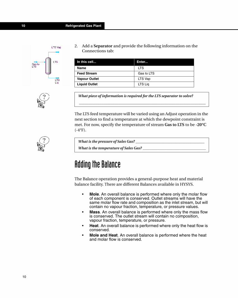
2. Add a Separator and provide the following information on the Connections tab:

The LTS feed temperature will be varied using an Adjust operation in the next section to find a temperature at which the dewpoint constraint is met. For now, specify the temperature of stream Gas to LTS to be -20°C (-4°F).

Adding the BalanceThe Balance operation provides a general-purpose heat and material balance facility. There are different Balances available in HYSYS.

• Mole. An overall balance is performed where only the molar flow of each component is conserved. Outlet streams will have the same molar flow rate and composition as the inlet stream, but will contain no vapour fraction, temperature, or pressure values.

• Mass. An overall balance is performed where only the mass flow is conserved. The outlet stream will contain no composition, vapour fraction, temperature, or pressure.

• Heat. An overall balance is performed where only the heat flow is conserved.

• Mole and Heat. An overall balance is performed where the heat and molar flow is conserved.


Name LTS

Feed Stream Gas to LTS

Vapour Outlet LTS Vap

Liquid Outlet LTS Liq

What piece of information is required for the LTS separator to solve?

____________________________________________________________________

What is the pressure of Sales Gas? _____________________________________

What is the temperature of Sales Gas? __________________________________

10


Look at the parameters for Sales Gas. The stream parameters are calculated so that there is no way you can force the stream to calculate a dewpoint temperature at 6000 kPa. Adding a Mole Balance allows you to create a second stream with the same molar flowrate and composition as Sales Gas but no vapour fraction, temperature, or pressure.

1. Double-click on the Balance icon on the Object Palette.

2. Add the following information on the Connections tab:

3. Specify a Pressure of 6000 kPa (870 psia) for the stream HC Dewpoint.

4. Set the Vapour Fraction to calculate the dew point temperature.


Inlet Stream Sales Gas

Outlet Stream HC Dewpoint

Type (on Parameters tab) Mole

What is the dewpoint temperature? ____________________________________

The required dewpoint is -15°C, is the current dewpoint higher or lower?

____________________________________________________________________

Assuming that pressure is fixed, what other parameter affects the dewpoint? ____________________________________________________________________

How can we change the dewpoint in the simulation? _____________________

Balance icon

11


Adding the AdjustThe Adjust operation is a Logical Operation; a mathematical operation rather than a physical operation. It will vary the value of one stream variable (the independent variable) to meet a required value or specification (the dependant variable) in another stream or operation.

1. Double-click on the Adjust icon on the Object Palette; the Adjust property view appears.

2. Click the Select Var... button in the Adjusted Variable group. The Variable Navigator view appears.

Figure 5Adjust icon

The Adjusted Variable must always be a user specified value.

12


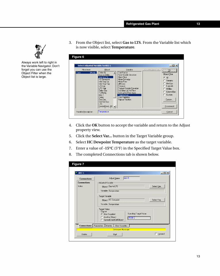
3. From the Object list, select Gas to LTS. From the Variable list which is now visible, select Temperature.

4. Click the OK button to accept the variable and return to the Adjust property view.

5. Click the Select Var... button in the Target Variable group.

6. Select HC Dewpoint Temperature as the target variable.

7. Enter a value of -15°C (5°F) in the Specified Target Value box.

8. The completed Connections tab is shown below.

Figure 6

Figure 7

Always work left to right in the Variable Navigator. Don’t forget you can use the Object Filter when the Object list is large.

13


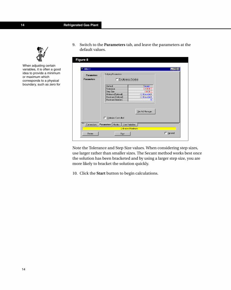
9. Switch to the Parameters tab, and leave the parameters at the default values.

Note the Tolerance and Step Size values. When considering step sizes, use larger rather than smaller sizes. The Secant method works best once the solution has been bracketed and by using a larger step size, you are more likely to bracket the solution quickly.

10. Click the Start button to begin calculations.

Figure 8

When adjusting certain variables, it is often a good idea to provide a minimum or maximum which corresponds to a physical boundary, such as zero for

14


11. To view the progress of the Adjust, go to the Monitor page.

Optional

Figure 9

What is the Chiller outlet temperature to achieve the Dewpoint specification? ______________________________________________________

Save your case!

Convert your case to a template and save!

15


Advanced Modeling

Linking the Propane Loop to the Gas PlantOnce you have completed the Refrigerated Gas Plant example, you can link it to the Propane Loop template.

The duty of the Chiller, Chiller Q, in the Gas Plant will be linked to the duty of the Chiller, Chill-Q, in the Propane Refrigeration Loop template.

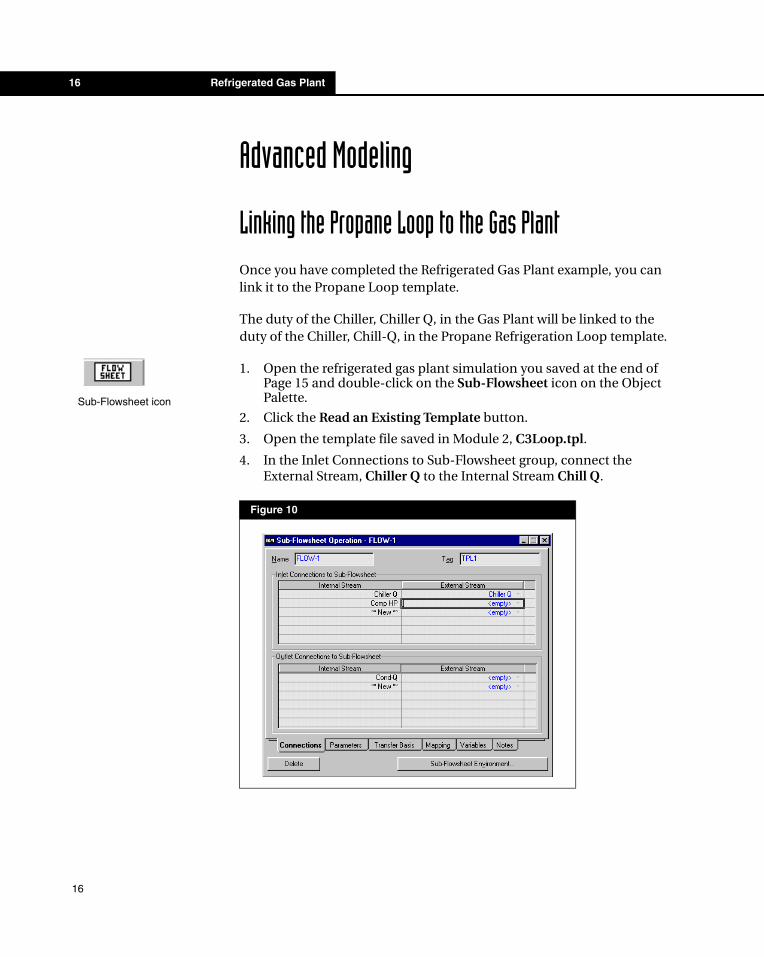
1. Open the refrigerated gas plant simulation you saved at the end of Page 15 and double-click on the Sub-Flowsheet icon on the Object Palette.

2. Click the Read an Existing Template button.

3. Open the template file saved in Module 2, C3Loop.tpl.

4. In the Inlet Connections to Sub-Flowsheet group, connect the External Stream, Chiller Q to the Internal Stream Chill Q.

Figure 10

Sub-Flowsheet icon

16


Once the connection is complete, both streams (internal and external) will have the same name (that of the external stream).

Exploring the Simulation

Exercise 1: Modifying the ExchangerThe available UA for the Gas-Gas Exchanger is only 2e5 kJ/°C.h. Make the necessary modifications to your exchanger design to achieve this UA.

ChallengeIn building the Refrigerated Gas Plant and the Propane Refrigeration Loop you decided to shortcut things and add a single-sided Cooler operation instead of the shell and tube exchanger that will actually be in the plant. This shortcut works for preliminary work, but now you need to replace the cooler with a shell and tube exchanger.

Remember, HYSYS allows you to attach streams from another flowsheet to either side of the heat exchanger. Using this feature, you should be able to solve this problem with only an exchanger in the Refrigerated Gas Plant (No exchanger in the Propane Refrigeration Loop).

What is the flowrate of propane in the Refrigeration Loop? _______________

How does this affect your LMTD and Temperature Approach? _____________

17


Using the Case StudyOpen the Starter case: Module3_CaseStudyStarter.hsc. This case is the solution to the Challenge problem in Module 2. The Case Study tool allows you to monitor the steady state response of key process variables to changes in your process. You select independent variables to change and dependent variables to monitor. HYSYS varies the independent variables one at a time, and with each change, the dependent variables are calculated.

The Economizer in the Propane Refrigeration loop results in a savings of energy over the single compression loop. The outlet pressure from the first stage compressor (Stream 4) has a significant effect on the total compression power required. We will use the Case Study to see the effect of changing the first stage compressor outlet pressure on the total power required by the refrigeration loop.

If your case contains any Adjust operations, they must be turned off so that they do not conflict with the Case Study.

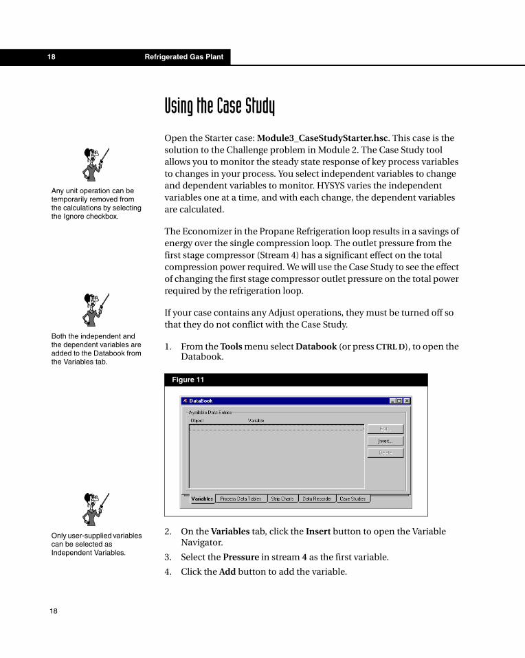
1. From the Tools menu select Databook (or press CTRL D), to open the Databook.

2. On the Variables tab, click the Insert button to open the Variable Navigator.

3. Select the Pressure in stream 4 as the first variable.

4. Click the Add button to add the variable.

Figure 11

Any unit operation can be temporarily removed from the calculations by selecting the Ignore checkbox.

Both the independent and the dependent variables are added to the Databook from the Variables tab.

Only user-supplied variables can be selected as Independent Variables.

18


5. Select the SPRDSHT-1, cell A3 and click Add. Click Close to close the Variable Navigator Window.

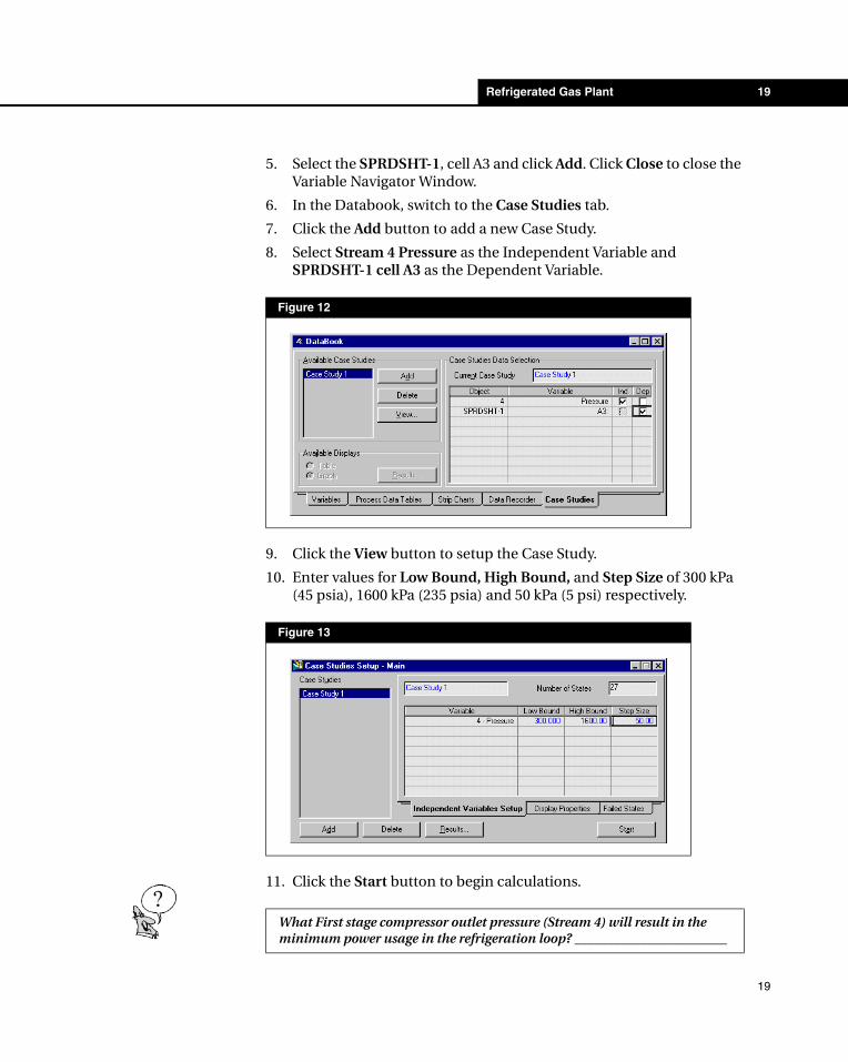
6. In the Databook, switch to the Case Studies tab.

7. Click the Add button to add a new Case Study.

8. Select Stream 4 Pressure as the Independent Variable and SPRDSHT-1 cell A3 as the Dependent Variable.

9. Click the View button to setup the Case Study.

10. Enter values for Low Bound, High Bound, and Step Size of 300 kPa (45 psia), 1600 kPa (235 psia) and 50 kPa (5 psi) respectively.

11. Click the Start button to begin calculations.

Figure 12

Figure 13

What First stage compressor outlet pressure (Stream 4) will result in the minimum power usage in the refrigeration loop? _______________________

19


20

03 refrigerated gasplant

Documents

Transcript of 03 refrigerated gasplant