02 WR6A-OM-E Rev G Body - Teledyne...
324
LECROY W AVERUNNER ® 6000A SERIES OSCILLOSCOPES OPERATOR’S MANUAL F EBRUARY 2007
Transcript of 02 WR6A-OM-E Rev G Body - Teledyne...
LECROY WAVERUNNER® 6000A
SERIES OSCILLOSCOPES
O P E R AT O R ’ S M A N U A L
FEBRUARY 2007

LeCroy Corporation 700 Chestnut Ridge Road Chestnut Ridge, NY 10977–6499 Tel: (845) 578 6020, Fax: (845) 578 5985
Internet: www.lecroy.com
© 2007 by LeCroy Corporation. All rights reserved.
LeCroy, ActiveDSO, WaveLink, JitterTrack, WavePro, WaveMaster, WaveSurfer, WaveExpert, WaveJet, and Waverunner are registered trademarks of LeCroy Corporation. Other product or brand names are trademarks or requested trademarks of their respective holders. Information in this publication supersedes all earlier versions. Specifications subject to change without notice.
Manufactured under an ISO 9000 Registered Quality Management System
Visit www.lecroy.com to view the certificate.
This electronic product is subject to disposal and recycling regulations that vary by country and region. Many countries prohibit the disposal of waste electronic equipment in standard waste receptacles.
For more information about proper disposal and recycling of your LeCroy product, please visit www.lecroy.com/recycle.
WR6A-OM-E Rev G
914871-00 Rev A
WR6A-OM-E Rev G 1
INTRODUCTION.................................................................................................13 How to Use On-line Help................................................................................................................13
Type Styles ............................................................................................................................. 13 Instrument Help....................................................................................................................... 13
Windows Help ................................................................................................................................14 Returning a Product for Service or Repair .....................................................................................14 Technical Support...........................................................................................................................14 Staying Up-to-Date.........................................................................................................................14 Windows License Agreement.........................................................................................................15 End-user License Agreement For LeCroy® X-Stream Software....................................................15 Virus Protection..............................................................................................................................21 Warranty.........................................................................................................................................21 Specifications .................................................................................................................................22
Vertical System....................................................................................................................... 22 Horizontal System................................................................................................................... 24 Acquisition System.................................................................................................................. 25 Acquisition Modes................................................................................................................... 25 Acquisition Processing............................................................................................................ 26 Triggering System................................................................................................................... 26 Basic Triggers ......................................................................................................................... 27 SMART Triggers ..................................................................................................................... 27 SMART Triggers with Exclusion Technology ......................................................................... 27 Automatic Setup...................................................................................................................... 27 Probes..................................................................................................................................... 27 Color Waveform Display ......................................................................................................... 28 Analog Persistence Display .................................................................................................... 28 Zoom Expansion Traces......................................................................................................... 28 Rapid Signal Processing......................................................................................................... 28 Internal Waveform Memory .................................................................................................... 28 Setup Storage......................................................................................................................... 28 Interface .................................................................................................................................. 28 Auxiliary Input ......................................................................................................................... 29 Auxiliary Output....................................................................................................................... 29 Math Tools (standard)............................................................................................................. 29 Measure Tools (standard)....................................................................................................... 30 Pass/Fail Testing .................................................................................................................... 30 Master Analysis Package (XMAP).......................................................................................... 30 Advanced Math Package (XMATH)........................................................................................ 30 Advanced Customization Package (XDEV)............................................................................ 31 Intermediate Math Package (XWAV)...................................................................................... 31 Jitter and Timing Analysis Package (JTA2)............................................................................ 31 Value Analysis Package (XVAP) ............................................................................................ 32 Web Editor (XWEB) ................................................................................................................ 32 Disk Drive Measurement Package (DDM2)............................................................................ 32 Digital Filter Package (DFP2) ................................................................................................. 33 Ethernet (ENET) ..................................................................................................................... 33 PowerMeasure Analyzer (PMA2) ........................................................................................... 33
WaveRunner 6000A Series Operator's Manual
2 WR6A-OM-E Rev G
USB2....................................................................................................................................... 33 Serial Data Manager ............................................................................................................... 35 General ................................................................................................................................... 35 Warranty and Service ............................................................................................................. 35 Environmental Characteristics ................................................................................................ 35 Temperature ........................................................................................................................... 35 Humidity .................................................................................................................................. 35 Altitude .................................................................................................................................... 35 Random Vibration ................................................................................................................... 36 Shock ...................................................................................................................................... 36
Certifications ................................................................................................................. 36 CE Declaration of Conformity ................................................................................................. 36 China RoHS Compliance........................................................................................................ 38
SAFETY REQUIREMENTS................................................................................40 Safety Symbols and Terms..................................................................................................... 40
Operating Environment ..................................................................................................................41 Cooling Requirements....................................................................................................................42 AC Power Source...........................................................................................................................42 Power and Ground Connections....................................................................................................42 On/Standby Switch.........................................................................................................................43 Calibration ......................................................................................................................................43 Cleaning .........................................................................................................................................43 Abnormal Conditions......................................................................................................................44 FRONT PANEL CONTROLS .............................................................................45 Front Panel Buttons and Knobs .....................................................................................................45
Trigger Knobs: ........................................................................................................................ 47 Trigger Buttons: ...................................................................................................................... 47 Horizontal Knobs:.................................................................................................................... 47 Vertical Knobs:........................................................................................................................ 47 Channel Buttons: .................................................................................................................... 47 Wavepilot Control Knobs: ...................................................................................................... 48 Special Features Buttons:...................................................................................................... 48 General Control Buttons: ....................................................................................................... 48
ON-SCREEN TOOLBARS, ICONS, AND DIALOG BOXES..............................49 Menu Bar Buttons ..........................................................................................................................49 Dialog Boxes ..................................................................................................................................50 Alternate Access Methods..............................................................................................................50 Mouse and Keyboard Operation ....................................................................................................50 Tool Bar Buttons.............................................................................................................................50 Trace Descriptors ...........................................................................................................................51 Trace Annotation ............................................................................................................................53
To Annotate a Waveform........................................................................................................ 53 To Turn On a Channel Trace Label ................................................................................................54 Screen Layout ................................................................................................................................55
WR6A-OM-E Rev G 3
Menu Bar ................................................................................................................................ 55 Signal Display Grid ................................................................................................................. 55
INSTALLATION..................................................................................................56 Hardware........................................................................................................................................56 External Monitor .............................................................................................................................56 Software .........................................................................................................................................57
Checking the Scope Status .................................................................................................... 57 Default Settings..............................................................................................................................58
WaveMaster and WavePro 7000 Series DSOs...................................................................... 58 DDA, SDA, and WaveRunner DSOs..............................................................................................58 Adding a New Option .....................................................................................................................58 Restoring Software.........................................................................................................................59
Restarting the Application....................................................................................................... 59 Restarting the Operating System............................................................................................ 60
Removable Hard Drive...................................................................................................................60 External Monitor .............................................................................................................................61 CONNECTING TO A SIGNAL ............................................................................63 ProBus Interface ............................................................................................................................63 Auxiliary Output Signals .................................................................................................................63 To Set Up Auxiliary Output .............................................................................................................63 SAMPLING MODES ...........................................................................................65 Sampling Modes ............................................................................................................................65
To Select a Sampling Mode.................................................................................................... 65 Single-shot sampling mode............................................................................................................65
Basic Capture Technique ....................................................................................................... 65 Sequence SAMPLING Mode Working With Segments..................................................................66
To Set Up Sequence Mode .................................................................................................... 67 Sequence Display Modes ....................................................................................................... 68 To Display Individual Segments ............................................................................................. 69 To View Time Stamps............................................................................................................. 69
RIS SAMPLING Mode -- For Higher Sample Rates ......................................................................70 Roll Mode .......................................................................................................................................70 VERTICAL SETTINGS AND CHANNEL CONTROLS .......................................71 Adjusting Sensitivity and Position ..................................................................................................71
To Adjust Sensitivity................................................................................................................ 71 To Adjust the Waveform's Position......................................................................................... 71
Coupling .........................................................................................................................................71 Overload Protection ................................................................................................................ 71 To Set Coupling ...................................................................................................................... 72
Probe Attenuation...........................................................................................................................72 To Set Probe Attenuation ....................................................................................................... 72
Bandwidth Limit ..............................................................................................................................72 To Set Bandwidth Limiting ...................................................................................................... 72
Linear and (SinX)/X Interpolation...................................................................................................72 To Set Up Interpolation........................................................................................................... 73

WaveRunner 6000A Series Operator's Manual
4 WR6A-OM-E Rev G
Inverting Waveforms............................................................................................................... 73 QuickZoom.....................................................................................................................................73
To Turn On a Zoom ................................................................................................................ 73 Finding Scale..................................................................................................................................73
To Use Find Scale .................................................................................................................. 73 Variable Gain..................................................................................................................................73
To Enable Variable Gain......................................................................................................... 73 Channel Deskew ............................................................................................................................74
To Set Up Channel Deskew ................................................................................................... 74 TIMEBASE AND ACQUISITION SYSTEM.........................................................75 Timebase Setup and Control .........................................................................................................75 Dual Channel Acquisition ...............................................................................................................75
Combining of Channels........................................................................................................... 75 To Combine Channels ............................................................................................................75
Autosetup .......................................................................................................................................76 TRIGGERING .....................................................................................................77 Trigger Setup Considerations ........................................................................................................77
Trigger Modes......................................................................................................................... 77 Trigger Types.......................................................................................................................... 77
Determining Trigger Level, Slope, Source, and Coupling..............................................................78 Trigger Source................................................................................................................................79 Level...............................................................................................................................................79 Holdoff by Time or Events ..............................................................................................................80
Hold Off by Time..................................................................................................................... 80 Hold Off by Events .................................................................................................................. 80
Simple Triggers ..............................................................................................................................81 Edge Trigger on Simple Signals ............................................................................................. 81 Control Edge Triggering.......................................................................................................... 81 To Set Up an Edge Trigger..................................................................................................... 82
SMART Triggers.............................................................................................................................84 Width Trigger .......................................................................................................................... 84 Glitch Trigger .......................................................................................................................... 85 Interval Trigger........................................................................................................................ 87 Qualified Trigger ..................................................................................................................... 91 State Trigger ........................................................................................................................... 93 Dropout Trigger....................................................................................................................... 95 Logic Trigger ........................................................................................................................... 96
DISPLAY FORMATS..........................................................................................98 Display Setup .................................................................................................................................98
Sequence Mode Display......................................................................................................... 98 Persistence Setup ..........................................................................................................................99
Saturation Level ...................................................................................................................... 99 3-Dimensional Persistence ................................................................................................... 100
Show Last Trace ..........................................................................................................................101 Persistence Time..........................................................................................................................101
WR6A-OM-E Rev G 5
Locking of Traces .........................................................................................................................101 To Set Up Persistence..................................................................................................................102 Screen Saver ...............................................................................................................................103 Moving Traces from Grid to Grid..................................................................................................103
To Move a Channel or Math Trace....................................................................................... 103 Zooming Waveforms ....................................................................................................................103
To Zoom a Single Channel ................................................................................................... 104 To Zoom by Touch-and-Drag ............................................................................................... 105 To Zoom Multiple Waveforms Quickly.................................................................................. 106 Multi-Zoom............................................................................................................................ 106
XY Display....................................................................................................................................108 To Set Up XY Displays ......................................................................................................... 108
SAVE AND RECALL ........................................................................................109 Saving and Recalling Scope Settings ..........................................................................................109
To Save Scope Settings ....................................................................................................... 109 To Recall Scope Settings ..................................................................................................... 109 To Recall Default Settings .................................................................................................... 109
Saving Screen Images ................................................................................................................. 110 Saving and Recalling Waveforms ................................................................................................ 110
Saving Waveforms................................................................................................................ 110 Recalling Waveforms............................................................................................................ 112
Disk Utilities.................................................................................................................................. 112 To Delete a Single File ......................................................................................................... 112 To Delete All Files in a Folder............................................................................................... 113 To Create a Folder................................................................................................................ 113
PRINTING AND FILE MANAGEMENT.............................................................114 Print, Plot, or Copy ....................................................................................................................... 114 Printing ......................................................................................................................................... 114
To Set Up the Printer ............................................................................................................ 114 To Print ................................................................................................................................. 114 Adding Printers and Drivers.................................................................................................. 114 Changing the Default Printer ................................................................................................ 115
Managing Files............................................................................................................................. 115 Hard Disk Partitions .............................................................................................................. 115
100BASE-T ETHERNET CONNECTION..........................................................116 Connecting to a Network.............................................................................................................. 116 Communicating over the Network................................................................................................ 116
Windows Setups ................................................................................................................... 117 Windows Repair Disk............................................................................................................ 117
TRACK VIEWS .................................................................................................118 Creating and Viewing a Trend...................................................................................................... 118 Creating a Track View .................................................................................................................. 119 HISTOGRAMS..................................................................................................120 Creating and Viewing a Histogram ..............................................................................................120
WaveRunner 6000A Series Operator's Manual
6 WR6A-OM-E Rev G
To Set Up a Single Parameter Histogram ............................................................................ 120 To View Thumbnail Histograms............................................................................................ 121 Persistence Histogram..........................................................................................................121 Persistence Trace Range .....................................................................................................122 Persistence Sigma................................................................................................................ 122
Histogram Parameters .................................................................................................................123 Histogram Theory of Operation....................................................................................................136
DSO Process ........................................................................................................................ 138 Parameter Buffer................................................................................................................... 138 Capture of Parameter Events ............................................................................................... 139
Histogram Parameters (XMAP and JTA2 Options)......................................................................139 Histogram Peaks..........................................................................................................................140 Binning and Measurement Accuracy ...........................................................................................141 WAVEFORM MEASUREMENTS .....................................................................142 Measuring with Cursors ...............................................................................................................142
Cursor Measurement Icons .................................................................................................. 142 Cursors Setup ..............................................................................................................................142
Quick Display ........................................................................................................................ 142 Full Setup.............................................................................................................................. 143
Overview of Parameters...............................................................................................................143 To Turn On Parameters........................................................................................................ 143 Quick Access to Parameter Setup Dialogs........................................................................... 143 Status Symbols ..................................................................................................................... 144 Using X-Stream Browser to Obtain Status Information ........................................................ 145
Statistics .......................................................................................................................................146 To Apply a Measure Mode............................................................................................................147 Measure Modes ...........................................................................................................................147
Standard Vertical Parameters............................................................................................... 147 Standard Horizontal Parameters .......................................................................................... 147 My Measure .......................................................................................................................... 148
Parameter Math (XMATH or XMAP option required) ...................................................................148 Logarithmic Parameters........................................................................................................ 148 Excluded Parameters............................................................................................................148 Parameter Script Parameter Math ........................................................................................ 149 Param Script vs. P Script ......................................................................................................150 To Set Up Parameter Math................................................................................................... 150 To Set Up Parameter Script Math......................................................................................... 150
Measure Gate...............................................................................................................................151 To Set Up Measure Gate...................................................................................................... 152
Help Markers................................................................................................................................153 To Set Up Help Markers ....................................................................................................... 155 To Turn Off Help Markers ..................................................................................................... 155
To Customize a Parameter...........................................................................................................155 From the Measure Dialog ..................................................................................................... 155 From a Vertical Setup Dialog................................................................................................ 156 From a Math Setup Dialog.................................................................................................... 156

WR6A-OM-E Rev G 7
Parameter Calculations................................................................................................................156 Parameters and How They Work.......................................................................................... 156 Determining Time Parameters.............................................................................................. 159 Determining Differential Time Measurements ...................................................................... 160 Level and Slope .................................................................................................................... 160
List of Parameters ........................................................................................................................161 WAVEFORM MATH..........................................................................................188 Introduction to Math Traces and Functions..................................................................................188 MATH MADE EASY .....................................................................................................................188
To Set Up a Math Function................................................................................................... 188 Resampling To Deskew................................................................................................................189
To Resample......................................................................................................................... 189 Rescaling and Assigning Units.....................................................................................................190
To Set Up Rescaling............................................................................................................. 190 Averaging Waveforms ..................................................................................................................190
Summed vs. Continuous Averaging ..................................................................................... 190 To Set Up Continuous Averaging ......................................................................................... 192 To Set Up Summed Averaging ............................................................................................. 192
Enhanced Resolution ...................................................................................................................192 How the Instrument Enhances Resolution ........................................................................... 193
To Set Up Enhanced Resolution (ERES).....................................................................................195 Waveform Copy............................................................................................................................195 Waveform Sparser........................................................................................................................196
To Set Up Waveform Sparser............................................................................................... 196 Interpolation .................................................................................................................................196
To Set Up Interpolation......................................................................................................... 196 FFT....................................................................................................................198 Why Use FFT? .............................................................................................................................198 Power (Density) Spectrum ...........................................................................................................198 FFT Pitfalls to Avoid .....................................................................................................................199 Picket Fence and Scallop.............................................................................................................199 Leakage........................................................................................................................................199 Choosing a Window .....................................................................................................................199 Improving Dynamic Range...........................................................................................................200 Record Length..............................................................................................................................201 FFT Algorithms.............................................................................................................................201 Glossary .......................................................................................................................................203 FFT Setup ....................................................................................................................................206
To Set Up an FFT ................................................................................................................. 206 ANALYSIS ........................................................................................................207 Pass/Fail Testing ..........................................................................................................................207
Comparing Parameters......................................................................................................... 207 Mask Tests............................................................................................................................ 208 Actions .................................................................................................................................. 208
Setting Up Pass/Fail Testing ........................................................................................................209
WaveRunner 6000A Series Operator's Manual
8 WR6A-OM-E Rev G
Initial Setup ........................................................................................................................... 209 Comparing a Single Parameter ............................................................................................ 209 Comparing Dual Parameters ................................................................................................ 211 Mask Testing......................................................................................................................... 212
UTILITIES.........................................................................................................213 Status ...........................................................................................................................................213
To Access Status Dialog....................................................................................................... 213 Remote communication ...............................................................................................................213
To Set Up Remote Communication. ..................................................................................... 213 To Configure the Remote Control Assistant Event Log........................................................ 213
Hardcopy......................................................................................................................................214 Printing.................................................................................................................................. 214 Clipboard............................................................................................................................... 214 File ........................................................................................................................................ 214 E-Mail .................................................................................................................................... 215
Aux Output ...................................................................................................................................215 Date & Time..................................................................................................................................216
To Set Time and Date Manually ........................................................................................... 216 To Set Time and Date from the Internet ............................................................................... 216 To Set Time and Date from Windows................................................................................... 216
Options .........................................................................................................................................217 Preferences..................................................................................................................................217
Audible Feedback ................................................................................................................. 217 Auto-calibration ..................................................................................................................... 218 Offset Control........................................................................................................................ 218 Delay Control ........................................................................................................................ 218 Trigger Counter..................................................................................................................... 218 Performance Optimization .................................................................................................... 219 E-mail .................................................................................................................................... 219
Acquisition Status.........................................................................................................................220 Service .........................................................................................................................................220 Show Windows Desktop ..............................................................................................................220 Touch Screen Calibration .............................................................................................................220 CUSTOMIZATION ............................................................................................221 Customizing Your Instrument .......................................................................................................221
Introduction ........................................................................................................................... 221 Solutions ............................................................................................................................... 221 Examples .............................................................................................................................. 222 What is Excel? ...................................................................................................................... 227 What is Mathcad? ................................................................................................................. 227 What is MATLAB?................................................................................................................. 227 What is VBS?........................................................................................................................ 227 What can you do with a customized instrument? ................................................................. 229
Calling Excel from Your Instrument..............................................................................................230 Calling Excel Directly from the Instrument............................................................................ 230
How to Select a Math Function Call .............................................................................................230
WR6A-OM-E Rev G 9
How to Select a Parameter Function Call ....................................................................................230 The Excel Control Dialog .............................................................................................................230 Entering a File Name ...................................................................................................................231 Organizing Excel sheets ..............................................................................................................231 Setting the Vertical Scale .............................................................................................................233 Trace Descriptors .........................................................................................................................233 Multiple Inputs and Outputs .........................................................................................................233 Examples......................................................................................................................................234
Simple Excel Example 1 ....................................................................................................... 234 Simple Excel Example 2 ....................................................................................................... 238 Examples of Excel Parameter Functions.............................................................................. 241 Examples of Excel Waveform Functions .............................................................................. 241 Exponential Decay Time Constant Excel Parameter (Excel Example 1) ............................. 242 Gated Parameter Using Excel (Excel Example 2)................................................................ 244 How Does this Work? ........................................................................................................... 245 Correlation Excel Waveform Function (Excel Example 3).................................................... 246 Multiple Traces on One Grid (Excel Example 4) .................................................................. 248 Using a Surface Plot (Excel Example 5)............................................................................... 251
Writing VB Scripts ........................................................................................................................252 Types of Scripts in VBS ........................................................................................................ 252 Loading and Saving VBScripts ............................................................................................. 253 The default parameter function script: explanatory notes .................................................... 256 Scripting with VBScript ......................................................................................................... 257 Variable Types...................................................................................................................... 258
Variable Names............................................................................................................................258 Arithmetic Operators ....................................................................................................................260 VBS Controls................................................................................................................................261
IF . . . Then . . . Else . . . End If ............................................................................................. 262 Summary of If . . . . Then . . . . Else ...................................................................................... 264 Select Case........................................................................................................................... 265 Summary of Select Case . . . . End Select ........................................................................... 265 Do . . . Loop .......................................................................................................................... 266 While . . . Wend..................................................................................................................... 266 For . . . Next .......................................................................................................................... 267
VBS keywords and functions .......................................................................................................268 Other VBS Words ................................................................................................................. 269
Functions......................................................................................................................................270 Hints and Tips for VBScripting .....................................................................................................271 ERRORS......................................................................................................................................272 Error Handling ..............................................................................................................................274 Speed of Execution ......................................................................................................................274 Scripting Ideas .............................................................................................................................275 Example Waveform Script............................................................................................................275 Example Parameter Scripts .........................................................................................................276 Debugging Scripts........................................................................................................................276 Horizontal Control Variables.........................................................................................................276 Vertical Control Variables .............................................................................................................276
WaveRunner 6000A Series Operator's Manual
10 WR6A-OM-E Rev G
List of Variables Available to Scripts ............................................................................................277 Communicating with Excel from a VBScript.................................................................................278 Calling MATLAB from the Instrument...........................................................................................279
Calling MATLAB.................................................................................................................... 279 How to Select a Waveform Function Call.....................................................................................280 The MATLAB Waveform Control Panel........................................................................................280 MATLAB Waveform Function Editor -- Example ..........................................................................282 MATLAB Example Waveform Plot................................................................................................284 How to Select a MATLAB Parameter Call....................................................................................285 The MATLAB Parameter Control Panel .......................................................................................285 The MATLAB Parameter Editor....................................................................................................286 MATLAB Example Parameter Panel ............................................................................................287 Further Examples of MATLAB Waveform Functions....................................................................289 Creating Your Own MATLAB Function.........................................................................................291 CUSTOMDSO...................................................................................................292 Custom DSO ................................................................................................................................292
Introduction – What is CustomDSO?.................................................................................... 292 Invoking CustomDSO ........................................................................................................... 292 CustomDSO Basic Mode...................................................................................................... 293 Editing a CustomDSO Setup File ......................................................................................... 293 Creating a CustomDSO Setup File....................................................................................... 295 CustomDSO PlugIn Mode .................................................................................................... 295 Creating a CustomDSO PlugIn............................................................................................. 295 Properties of the Control and its Objects .............................................................................. 297 Removing a PlugIn................................................................................................................ 301 First Example PlugIn – Exchanging Two Traces on the Grids ............................................. 301 Second Example PlugIn – Log-Log FFT Plot ....................................................................... 304 Control Variables in CustomDSO ......................................................................................... 306
PROCESSING WEB OPTION..........................................................................307 To Use the Web Editor .................................................................................................................307
Adding Parameters ............................................................................................................... 309 Adding Previews ................................................................................................................... 310 Exiting the Web Editor .......................................................................................................... 310 Viewing the Output................................................................................................................ 310
LABNOTEBOOK..............................................................................................311 Introduction to LabNotebook ................................................................................................. 311 Preferences ................................................................................................................................ 311
Miscellaneous Settings .........................................................................................................311 Hardcopy Setup .................................................................................................................... 312 E-mail Setup ......................................................................................................................... 312
Creating a Notebook Entry .....................................................................................................312 Recalling Notebook Entries .....................................................................................................317 Creating a Report .....................................................................................................................318
Previewing a Report.............................................................................................................. 318 Locating a Notebook Entry ................................................................................................... 318

WR6A-OM-E Rev G 11
Creating the Report......................................................................................................................319 Formatting the Report ..................................................................................................................319 Managing Notebook Entry Data.............................................................................................320
Adding Annotations............................................................................................................... 320 Deleting Notebook Entries .................................................................................................... 320 Saving Notebook Entries to a Folder.................................................................................... 321 Managing the Database........................................................................................................ 321 To Start a New Database ..................................................................................................... 322
WaveRunner 6000A Series Operator's Manual
12 WR6A-OM-E Rev G
BLANK PAGE

WR6A-OM-E Rev G 13
INTRODUCTION How to Use On-line Help Type Styles
Activators of pop-up text and images appear as green, underlined, italic: Pop-up. To close pop-up text and images after opening them, touch the pop-up text again.
Links jump you to other topics, URLs, or images. They take you out of the current Help screen. Link text appears blue and underlined: Link. After making a jump, you can touch the Back icon in the toolbar at the top of the Help window to return to the Help screen you just left. With each touch of the Back icon, you return to the preceding Help screen. Instrument Help
When you press the front panel Help button (if available), or touch the on-screen Help
button , you will be presented with a menu: you can choose either to have information found for you automatically or to search for information yourself.
If you want context-sensitive Help, that is, Help related to what was displayed on the screen when
you requested Help, touch in the drop-down menu, then touch the on-screen control (or front panel button or knob) that you need information about. The instrument will automatically display Help about that control.
If you want information about something not displayed on the screen, touch one of the buttons inside the drop-down menu to display the on-line Help manual:
Contents displays the Table of Contents.
Index displays an alphabetical listing of keywords.
Search locates every occurrence of the keyword that you enter.
www.LeCroy.com connects you to LeCroy's Web site where you can find Lab Briefs, Application Notes, and other useful information. This feature requires that the instrument be connected to the internet through the Ethernet port on the scope's rear panel. Refer to Remote Communication for setup instructions.
About opens the Utilities "Status" dialog, which shows software version and other system information.
WaveRunner 6000A Series Operator's Manual
14 WR6A-OM-E Rev G
Once opened, the Help window will display its navigation pane: the part of the window that shows the Table of Contents and Index. When you touch anywhere outside of the Help window, this navigation pane will disappear to reveal more of your signal. To make it return, touch the Show
icon at the top of the Help window or touch inside the Help information pane.
Windows Help In addition to instrument Help, you can also access on-line Help for Microsoft® Windows®. This help is accessible by minimizing the scope application, then touching the Start button in the Windows task bar at the bottom of the screen and selecting Help.
Returning a Product for Service or Repair If you need to return a LeCroy product, identify it by its model and serial numbers. Describe the defect or failure, and give us your name and telephone number.
For factory returns, use a Return Authorization Number (RAN), which you can get from customer service. Write the number clearly on the outside of the shipping carton.
Return products requiring only maintenance to your local customer service center.
If you need to return your scope for any reason, use the original shipping carton. If this is not possible, be sure to use a rigid carton. The scope should be packed so that it is surrounded by a minimum of four inches (10 cm) of shock absorbent material.
Within the warranty period, transportation charges to the factory will be your responsibility. Products under warranty will be returned to you with transport prepaid by LeCroy. Outside the warranty period, you will have to provide us with a purchase order number before the work can be done. You will be billed for parts and labor related to the repair work, as well as for shipping.
You should prepay return shipments. LeCroy cannot accept COD (Cash On Delivery) or Collect Return shipments. We recommend using air freight.
Technical Support You can get assistance with installation, calibration, and a full range of software applications from your customer service center. Visit the LeCroy Web site at http://www.lecroy.com for the center nearest you.
Staying Up-to-Date To maintain your instrument’s performance within specifications, have us calibrate it at least once a year. LeCroy offers state-of-the-art performance by continually refining and improving the instrument’s capabilities and operation. We frequently update both firmware and software during service, free of charge during warranty.
You can also install new purchased software options in your scope yourself, without having to return it to the factory. Simply provide us with your instrument serial number and ID, and the version number of instrument software installed. We will provide you with a unique option key that consists of a code to be entered through the Utilities' Options dialog to load the software option.
WR6A-OM-E Rev G 15
Windows License Agreement LeCroy's agreement with Microsoft prohibits users from running software on LeCroy X-Stream oscilloscopes that is not relevant to measuring, analyzing, or documenting waveforms.
End-user License Agreement For LeCroy® X-Stream Software IMPORTANT-READ CAREFULLY: THIS END-USER LICENSE AGREEMENT (“EULA”) IS A LEGAL AGREEMENT BETWEEN THE INDIVIDUAL OR ENTITY LICENSING THE SOFTWARE PRODUCT (“YOU” OR “YOUR”) AND LECROY CORPORATION (“LECROY”) FOR THE SOFTWARE PRODUCT(S) ACCOMPANYING THIS EULA, WHICH INCLUDE(S): COMPUTER PROGRAMS; ANY “ONLINE” OR ELECTRONIC DOCUMENTATION AND PRINTED MATERIALS PROVIDED BY LECROY HEREWITH (“DOCUMENTATION”); ASSOCIATED MEDIA; AND ANY UPDATES (AS DEFINED BELOW) (COLLECTIVELY, THE “SOFTWARE PRODUCT”). BY USING AN INSTRUMENT TOGETHER WITH OR CONTAINING THE SOFTWARE PRODUCT, OR BY INSTALLING, COPYING, OR OTHERWISE USING THE SOFTWARE PRODUCT, IN WHOLE OR IN PART, YOU AGREE TO BE BOUND BY THE TERMS OF THIS EULA. IF YOU DO NOT AGREE TO THE TERMS OF THIS EULA, DO NOT INSTALL, COPY, OR OTHERWISE USE THE SOFTWARE PRODUCT; YOU MAY RETURN THE SOFTWARE PRODUCT TO YOUR PLACE OF PURCHASE FOR A FULL REFUND. IN ADDITION, BY INSTALLING, COPYING, OR OTHERWISE USING ANY MODIFICATIONS, ENHANCEMENTS, NEW VERSIONS, BUG FIXES, OR OTHER COMPONENTS OF THE SOFTWARE PRODUCT THAT LECROY PROVIDES TO YOU SEPARATELY AS PART OF THE SOFTWARE PRODUCT (“UPDATES”), YOU AGREE TO BE BOUND BY ANY ADDITIONAL LICENSE TERMS THAT ACCOMPANY SUCH UPDATES. IF YOU DO NOT AGREE TO SUCH ADDITIONAL LICENSE TERMS, YOU MAY NOT INSTALL, COPY, OR OTHERWISE USE SUCH UPDATES.
THE PARTIES CONFIRM THAT THIS AGREEMENT AND ALL RELATED DOCUMENTATION ARE AND WILL BE DRAFTED IN ENGLISH. LES PARTIES AUX PRÉSENTÉS CONFIRMENT LEUR VOLONTÉ QUE CETTE CONVENTION DE MÊME QUE TOUS LES DOCUMENTS Y COMPRIS TOUT AVIS QUI S’Y RATTACHÉ, SOIENT REDIGÉS EN LANGUE ANGLAISE.
1. GRANT OF LICENSE.
1.1 License Grant. Subject to the terms and conditions of this EULA and payment of all applicable fees, LeCroy grants to you a nonexclusive, nontransferable license (the “License”) to: (a) operate the Software Product as provided or installed, in object code form, for your own internal business purposes, (i) for use in or with an instrument provided or manufactured by LeCroy (an “Instrument”), (ii) for testing your software product(s) (to be used solely by you) that are designed to operate in conjunction with an Instrument (“Your Software”), and (iii) make one copy for archival and back-up purposes; (b) make and use copies of the Documentation; provided that such copies will be used only in connection with your licensed use of the Software Product, and such copies may not be republished or distributed (either in hard copy or electronic form) to any third party; and (c) copy, modify, enhance and prepare derivative works (“Derivatives”) of the source code version of those portions of the Software Product set forth in and identified in the Documentation as “Samples” (“Sample Code”) for the sole purposes of designing, developing, and testing Your Software. If you are an entity, only one designated individual within your organization, as designated by you, may exercise the License; provided that additional individuals

WaveRunner 6000A Series Operator's Manual
16 WR6A-OM-E Rev G
within your organization may assist with respect to reproducing and distributing Sample Code as permitted under Section 1.1(c)(ii). LeCroy reserves all rights not expressly granted to you. No license is granted hereunder for any use other than that specified herein, and no license is granted for any use in combination or in connection with other products or services (other than Instruments and Your Software) without the express prior written consent of LeCroy. The Software Product is licensed as a single product. Its component parts may not be separated for use by more than one user. This EULA does not grant you any rights in connection with any trademarks or service marks of LeCroy. The Software Product is protected by copyright laws and international copyright treaties, as well as other intellectual property laws and treaties. The Software Product is licensed, not sold. The terms of this printed, paper EULA supersede the terms of any on-screen license agreement found within the Software Product.
1.2 Upgrades. If the Software Product is labeled as an “upgrade,” (or other similar designation) the License will not take effect, and you will have no right to use or access the Software Product unless you are properly licensed to use a product identified by LeCroy as being eligible for the upgrade (“Underlying Product”). A Software Product labeled as an “upgrade” replaces and/or supplements the Underlying Product. You may use the resulting upgraded product only in accordance with the terms of this EULA. If the Software Product is an upgrade of a component of a package of software programs that you licensed as a single product, the Software Product may be used and transferred only as part of that single product package and may not be separated for use on more than one computer.
1.3. Limitations. Except as specifically permitted in this EULA, you will not directly or indirectly (a) use any Confidential Information to create any software or documentation that is similar to any of the Software Product or Documentation; (b) encumber, transfer, rent, lease, time-share or use the Software Product in any service bureau arrangement; (c) copy (except for archival purposes), distribute, manufacture, adapt, create derivative works of, translate, localize, port or otherwise modify the Software Product or the Documentation; (d) permit access to the Software Product by any party developing, marketing or planning to develop or market any product having functionality similar to or competitive with the Software Product; (e) publish benchmark results relating to the Software Product, nor disclose Software Product features, errors or bugs to third parties; or (f) permit any third party to engage in any of the acts proscribed in clauses (a) through (e). In jurisdictions in which transfer is permitted, notwithstanding the foregoing prohibition, transfers will only be effective if you transfer a copy of this EULA, as well as all copies of the Software Product, whereupon your right to use the Software product will terminate. Except as described in this Section 1.3, You are not permitted (i) to decompile, disassemble, reverse compile, reverse assemble, reverse translate or otherwise reverse engineer the Software Product, (ii) to use any similar means to discover the source code of the Software Product or to discover the trade secrets in the Software Product, or (iii) to otherwise circumvent any technological measure that controls access to the Software Product. You may reverse engineer or otherwise circumvent the technological measures protecting the Software Product for the sole purpose of identifying and analyzing those elements that are necessary to achieve Interoperability (the “Permitted Objective”) only if: (A) doing so is necessary to achieve the Permitted Objective and it does not constitute infringement under Title 17 of the United States Code; (B) such circumvention is confined to those parts of the Software Product and to such acts as are necessary to achieve the Permitted Objective; (C) the information to be gained thereby has not already been made readily available to you or has not been provided by LeCroy within a reasonable time after a written request by you to LeCroy to provide such information; (D) the information gained is not used for

WR6A-OM-E Rev G 17
any purpose other than the Permitted Objective and is not disclosed to any other person except as may be necessary to achieve the Permitted Objective; and (E) the information obtained is not used (1) to create a computer program substantially similar in its expression to the Software Product including, but not limited to, expressions of the Software Product in other computer languages, or (2) for any other act restricted by LeCroy’s intellectual property rights in the Software Product. “Interoperability” will have the same meaning in this EULA as defined in the Digital Millennium Copyright Act, 17 U.S.C. §1201(f), the ability of computer programs to exchange information and of such programs mutually to use the information which has been exchanged.
1.4 PRERELEASE CODE. Portions of the Software Product may be identified as prerelease code (“Prerelease Code”). Prerelease Code is not at the level of performance and compatibility of the final, generally available product offering. The Prerelease Code may not operate correctly and may be substantially modified prior to first commercial shipment. LeCroy is not obligated to make this or any later version of the Prerelease Code commercially available. The License with respect to the Prerelease Code terminates upon availability of a commercial release of the Prerelease Code from LeCroy.
2. SUPPORT SERVICES.
At LeCroy’s sole discretion, from time to time, LeCroy may provide Updates to the Software Product. LeCroy shall have no obligation to revise or update the Software Product or to support any version of the Software Product. At LeCroy’s sole discretion, upon your request, LeCroy may provide you with support services related to the Software Product (“Support Services”) pursuant to the LeCroy policies and programs described in the Documentation or otherwise then in effect, and such Support Services will be subject to LeCroy’s then-current fees therefor, if any. Any Update or other supplemental software code provided to you pursuant to the Support Services will be considered part of the Software Product and will be subject to the terms and conditions of this EULA. LeCroy may use any technical information you provide to LeCroy during LeCroy’s provision of Support Services, for LeCroy’s business purposes, including for product support and development. LeCroy will not utilize such technical information in a form that personally identifies you.
3. PROPRIETARY RIGHTS.
3.1 Right and Title. All right, title and interest in and to the Software Product and Documentation (including but not limited to any intellectual property or other proprietary rights, images, icons, photographs, text, and “applets” embodied in or incorporated into the Software Product, collectively, “Content”), and all Derivatives, and any copies thereof are owned by LeCroy and/or its licensors or third-party suppliers, and is protected by applicable copyright or other intellectual property laws and treaties. You will not take any action inconsistent with such title and ownership. This EULA grants you no rights to use such Content outside of the proper exercise of the license granted hereunder, and LeCroy will not be responsible or liable therefor.
3.2 Intellectual Property Protection. You may not alter or remove any printed or on-screen copyright, trade secret, proprietary or other legal notices contained on or in copies of the Software Product or Documentation.
3.3 Confidentiality. Except for the specific rights granted by this EULA, neither party shall use or disclose any Confidential Information (as defined below) of the other party without the written
WaveRunner 6000A Series Operator's Manual
18 WR6A-OM-E Rev G
consent of the disclosing party. A party receiving Confidential Information from the other shall use the highest commercially reasonable degree of care to protect the Confidential Information, including ensuring that its employees and consultants with access to such Confidential Information have agreed in writing not to disclose the Confidential Information. You shall bear the responsibility for any breaches of confidentiality by your employees and consultants. Within ten (10) days after request of the disclosing party, and in the disclosing party's sole discretion, the receiving party shall either return to the disclosing party originals and copies of any Confidential Information and all information, records and materials developed therefrom by the receiving party, or destroy the same, other than such Confidential Information as to which this EULA expressly provides a continuing right to the receiving party to retain at the time of the request. Either party may only disclose the general nature, but not the specific financial terms, of this EULA without the prior consent of the other party; provided either party may provide a copy of this EULA to any finance provider in conjunction with a financing transaction, if such provider agrees to keep this EULA confidential. Nothing herein shall prevent a receiving party from disclosing all or part of the Confidential Information as necessary pursuant to the lawful requirement of a governmental agency or when disclosure is required by operation of law; provided that prior to any such disclosure, the receiving party shall use reasonable efforts to (a) promptly notify the disclosing party in writing of such requirement to disclose, and (b) cooperate fully with the disclosing party in protecting against any such disclosure or obtaining a protective order. Money damages will not be an adequate remedy if this Section 4.3 is breached and, therefore, either party shall, in addition to any other legal or equitable remedies, be entitled to seek an injunction or similar equitable relief against such breach or threatened breach without the necessity of posting any bond. As used herein, “Confidential Information” means LeCroy pricing or information concerning new LeCroy products, trade secrets (including without limitation all internal header information contained in or created by the Software Product, all benchmark and performance test results and all Documentation) and other proprietary information of LeCroy; and any business, marketing or technical information disclosed by LeCroy, or its representatives, or you in relation to this EULA, and either (i) disclosed in writing and marked as confidential at the time of disclosure or (ii) disclosed in any other manner such that a reasonable person would understand the nature and confidentiality of the information. Confidential Information does not include information (A) already in the possession of the receiving party without an obligation of confidentiality to the disclosing party, (B) hereafter rightfully furnished to the receiving party by a third party without a breach of any separate nondisclosure obligation to the disclosing party, (C) publicly known without breach of this EULA, (d) furnished by the disclosing party to a third party without restriction on subsequent disclosure, or (e) independently developed by the receiving party without reference to or reliance on the Confidential Information.
4. TERMINATION.
This EULA will remain in force until termination pursuant to the terms hereof. You may terminate this EULA at any time. This EULA will also terminate if you breach any of the terms or conditions of this EULA. You agree that if this EULA terminates for any reason, the License will immediately terminate and you will destroy all copies of the Software Product (and all Derivatives), installed or otherwise, the Documentation, and the Confidential Information (and all derivatives of any of the foregoing) that are in your possession or under your control. The provisions of Sections 1.3, 4, 6, 7, 8, and 9 will survive any termination or expiration hereof.
5. U.S. GOVERNMENT RESTRICTED RIGHTS.
WR6A-OM-E Rev G 19
If any Software Product or Documentation is acquired by or on behalf of a unit or agency of the United States Government (any such unit or agency, the “Government”), the Government agrees that the Software Product or Documentation is “commercial computer software” or “commercial computer software documentation” and that, absent a written agreement to the contrary, the Government’s rights with respect to the Software Product or Documentation are, in the case of civilian agency use, Restricted Rights, as defined in FAR §52.227.19, and if for Department of Defense use, limited by the terms of this EULA, pursuant to DFARS §227.7202. The use of the Software Product or Documentation by the Government constitutes acknowledgment of LeCroy’s proprietary rights in the Software Product and Documentation. Manufacturer is LeCroy Corporation, 700 Chestnut Ridge Road, Chestnut Ridge, NY 10977 USA.
6. EXPORT RESTRICTIONS. You agree that you will not export or re-export the Software Product, any part thereof, or any process or service that is the direct product of the Software Product (the foregoing collectively referred to as the “Restricted Components”), to any country, person, entity or end user subject to U.S. export restrictions. You specifically agree not to export or re-export any of the Restricted Components (a) to any country to which the U.S. has embargoed or restricted the export of goods or services, which currently include, but are not necessarily limited to Cuba, Iran, Iraq, Libya, North Korea, Sudan and Syria, or to any national of any such country, wherever located, who intends to transmit or transport the Restricted Components back to such country; (b) to any end user who you know or have reason to know will utilize the Restricted Components in the design, development or production of nuclear, chemical or biological weapons; or (c) to any end-user who has been prohibited from participating in U.S. export transactions by any federal agency of the U.S. government. You warrant and represent that neither the BXA nor any other U.S. federal agency has suspended, revoked or denied your export privileges. It is your responsibility to comply with the latest United States export regulations, and you will defend and indemnify LeCroy from and against any damages, fines, penalties, assessments, liabilities, costs and expenses (including reasonable attorneys' fees and court costs) arising out of any claim that the Software Product, Documentation, or other information or materials provided by LeCroy hereunder were exported or otherwise accessed, shipped or transported in violation of applicable laws and regulations.
7. RISK ALLOCATION. 7.1 No Warranty. THE SOFTWARE PRODUCT IS NOT ERROR-FREE AND THE SOFTWARE PRODUCT AND SUPPORT SERVICES IS/ARE BEING PROVIDED "AS IS" WITHOUT WARRANTY OF ANY KIND. LECROY, FOR ITSELF AND ITS SUPPLIERS, HEREBY DISCLAIMS ALL WARRANTIES, WHETHER EXPRESS OR IMPLIED, ORAL OR WRITTEN, WITH RESPECT TO THE SOFTWARE PRODUCT OR ANY SUPPORT SERVICES INCLUDING, WITHOUT LIMITATION, ALL IMPLIED WARRANTIES OF TITLE OR NON-INFRINGEMENT, MERCHANTABILITY, FITNESS FOR A PARTICULAR PURPOSE, ACCURACY, INTEGRATION, VALIDITY, EXCLUSIVITY, MERCHANTABILITY, NON-INTERFERENCE WITH ENJOYMENT, FITNESS FOR ANY PARTICULAR PURPOSE, AND ALL WARRANTIES IMPLIED FROM ANY COURSE OF DEALING OR USAGE OF TRADE. YOU ACKNOWLEDGE THAT NO WARRANTIES HAVE BEEN MADE TO YOU BY OR ON BEHALF OF LECROY OR OTHERWISE FORM THE BASIS FOR THE BARGAIN BETWEEN THE PARTIES.
7.2. Limitation of Liability. LECROY’S LIABILITY FOR DAMAGES FOR ANY CAUSE WHATSOEVER, REGARDLESS OF THE FORM OF ANY CLAIM OR ACTION, SHALL NOT
WaveRunner 6000A Series Operator's Manual
20 WR6A-OM-E Rev G
EXCEED THE GREATER OF THE AMOUNT ACTUALLY PAID BY YOU FOR THE SOFTWARE PRODUCT OR U.S.$5.00; PROVIDED THAT IF YOU HAVE ENTERED INTO A SUPPORT SERVICES AGREEMENT WITH LECROY, LECROY’S ENTIRE LIABILITY REGARDING SUPPORT SERVICES WILL BE GOVERNED BY THE TERMS OF THAT AGREEMENT. LECROY SHALL NOT BE LIABLE FOR ANY LOSS OF PROFITS, LOSS OF USE, LOSS OF DATA, INTERRUPTION OF BUSINESS, NOR FOR INDIRECT, SPECIAL, INCIDENTAL, CONSEQUENTIAL OR EXEMPLARY DAMAGES OF ANY KIND, WHETHER UNDER THIS EULA OR OTHERWISE ARISING IN ANY WAY IN CONNECTION WITH THE SOFTWARE PRODUCT, THE DOCUMENTATION OR THIS EULA. SOME JURISDICTIONS DO NOT ALLOW THE EXCLUSION OR LIMITATION OF INCIDENTAL OR CONSEQUENTIAL DAMAGES, SO THE ABOVE EXCLUSION OR LIMITATION MAY NOT APPLY TO YOU. THESE LIMITATIONS ARE INDEPENDENT FROM ALL OTHER PROVISIONS OF THIS EULA AND SHALL APPLY NOTWITHSTANDING THE FAILURE OF ANY REMEDY PROVIDED HEREIN.
7.3 Indemnification. You will defend, indemnify and hold harmless LeCroy and its officers, directors, affiliates, contractors, agents, and employees from, against and in respect of any and all assessments, damages, deficiencies, judgments, losses, obligations and liabilities (including costs of collection and reasonable attorneys’ fees, expert witness fees and expenses) imposed upon or suffered or incurred by them arising from or related to your use of the Software Product.
8. GENERAL PROVISIONS.
8.1 Compliance with Laws. You will comply with all laws, legislation, rules, regulations, and governmental requirements with respect to the Software Product, and the performance by you of your obligations hereunder, of any jurisdiction in or from which you directly or indirectly cause the Software Product to be used or accessed.
8.2 No Agency. Nothing contained in this EULA will be deemed to constitute either party as the agent or representative of the other party, or both parties as joint venturers or partners for any purpose.
8.3 Entire Agreement; Waiver; Severability. This EULA constitutes the entire agreement between the parties with regard to the subject matter hereof. No provision of, right, power or privilege under this EULA will be deemed to have been waived by any act, delay, omission or acquiescence by LeCroy, its agents, or employees, but only by an instrument in writing signed by an authorized officer of LeCroy. No waiver by LeCroy of any breach or default of any provision of this EULA by you will be effective as to any other breach or default, whether of the same or any other provision and whether occurring prior to, concurrent with, or subsequent to the date of such waiver. If any provision of this EULA is declared by a court of competent jurisdiction to be invalid, illegal or unenforceable, such provision will be severed from this EULA and all the other provisions will remain in full force and effect.
8.4 Governing Law; Jurisdiction; Venue. This EULA will be governed by and construed in accordance with the laws of the State of New York, USA, without regard to its choice of law provisions. The United Nations Convention on Contracts for the International Sale of Goods will not apply to this EULA. Exclusive jurisdiction and venue for any litigation arising under this EULA is in the federal and state courts located in New York, New York, USA and both parties hereby consent to such jurisdiction and venue for this purpose.
WR6A-OM-E Rev G 21
8.5 Assignment. This EULA and the rights and obligations hereunder, may not be assigned, in whole or in part by you, except to a successor to the whole of your business, without the prior written consent of LeCroy. In the case of any permitted assignment or transfer of or under this EULA, this EULA or the relevant provisions will be binding upon, and inure to the benefit of, the successors, executors, heirs, representatives, administrators and assigns of the parties hereto.
8.6 Notices. All notices or other communications between LeCroy and you under this EULA will be in writing and delivered personally, sent by confirmed fax, by confirmed e-mail, by certified mail, postage prepaid and return receipt requested, or by a nationally recognized express delivery service. All notices will be in English and will be effective upon receipt.
8.7 Headings. The headings used in this EULA are intended for convenience only and will not be deemed to supersede or modify any provisions.
8.8 Acknowledgment. Licensee acknowledges that (a) it has read and understands this EULA, (b) it has had an opportunity to have its legal counsel review this EULA, (c) this EULA has the same force and effect as a signed agreement, and (d) issuance of this EULA does not constitute general publication of the Software Product or other Confidential Information.
Virus Protection Because your scope runs on a Windows-based PC platform, it must be protected from viruses, as with any PC on a corporate network. It is crucial that the scope be kept up to date with Windows Critical Updates, and that anti-virus software be installed and continually updated.
Visit http://www.lecroy.com/dsosecurity for more information regarding Windows Service Pack compatibility with LeCroy operating software, and related matters.
Warranty The instrument is warranted for normal use and operation, within specifications, for a period of three years from shipment. LeCroy will either repair or, at our option, replace any product returned to one of our authorized service centers within this period. However, in order to do this we must first examine the product and find that it is defective due to workmanship or materials and not due to misuse, neglect, accident, or abnormal conditions or operation.
LeCroy shall not be responsible for any defect, damage, or failure caused by any of the following: a) attempted repairs or installations by personnel other than LeCroy representatives, or b) improper connection to incompatible equipment or c) for any damage or malfunction caused by the use of non-LeCroy supplies. Furthermore, LeCroy shall not be obligated to service a product that has been modified or integrated where the modification or integration increases the task duration or difficulty of servicing the oscilloscope. Spare and replacement parts, and repairs, all have a 90-day warranty.
The oscilloscope’s firmware has been thoroughly tested and is presumed to be functional. Nevertheless, it is supplied without warranty of any kind covering detailed performance. Products not made by LeCroy are covered solely by the warranty of the original equipment manufacturer.
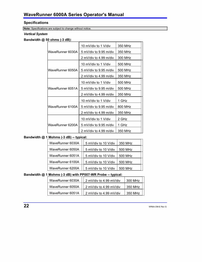
WaveRunner 6000A Series Operator's Manual
22 WR6A-OM-E Rev G
Specifications Note: Specifications are subject to change without notice.
Vertical System
Bandwidth @ 50 ohms (-3 dB):
WaveRunner 6030A
10 mV/div to 1 V/div 350 MHz
5 mV/div to 9.95 m/div 350 MHz
2 mV/div to 4.99 m/div 300 MHz
WaveRunner 6050A
10 mV/div to 1 V/div 500 MHz
5 mV/div to 9.95 m/div 500 MHz
2 mV/div to 4.99 m/div 350 MHz
WaveRunner 6051A
10 mV/div to 1 V/div 500 MHz
5 mV/div to 9.95 m/div 500 MHz
2 mV/div to 4.99 m/div 350 MHz
WaveRunner 6100A
10 mV/div to 1 V/div 1 GHz
5 mV/div to 9.95 m/div 800 MHz
2 mV/div to 4.99 m/div 350 MHz
WaveRunner 6200A
10 mV/div to 1 V/div 2 GHz
5 mV/div to 9.95 m/div 1 GHz
2 mV/div to 4.99 m/div 350 MHz Bandwidth @ 1 Mohms (-3 dB) -- typical:
WaveRunner 6030A 5 mV/div to 10 V/div 350 MHz WaveRunner 6050A 5 mV/div to 10 V/div 500 MHz WaveRunner 6051A 5 mV/div to 10 V/div 500 MHz WaveRunner 6100A 5 mV/div to 10 V/div 500 MHz WaveRunner 6200A 5 mV/div to 10 V/div 500 MHz
Bandwidth @ 1 Mohms (-3 dB) with PP007-WR Probe -- typical:
WaveRunner 6030A 2 mV/div to 4.99 mV/div 300 MHz WaveRunner 6050A 2 mV/div to 4.99 mV/div 350 MHz WaveRunner 6051A 2 mV/div to 4.99 mV/div 350 MHz
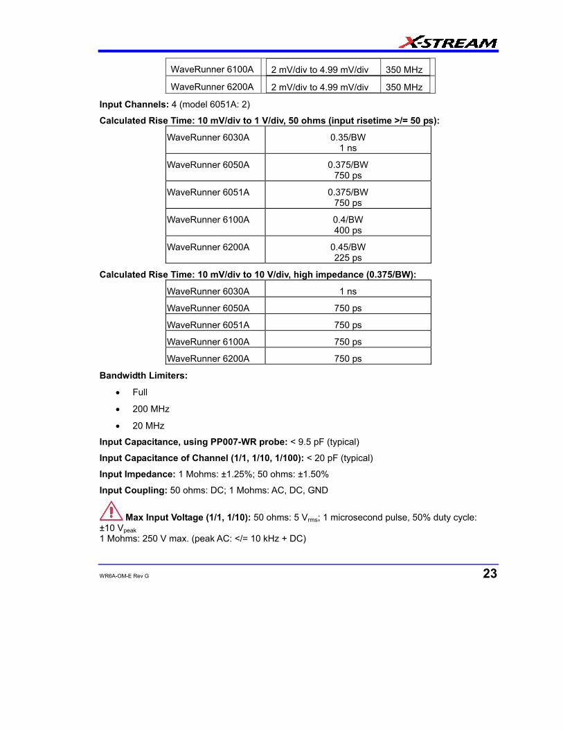
WR6A-OM-E Rev G 23
WaveRunner 6100A 2 mV/div to 4.99 mV/div 350 MHz WaveRunner 6200A 2 mV/div to 4.99 mV/div 350 MHz
Input Channels: 4 (model 6051A: 2)
Calculated Rise Time: 10 mV/div to 1 V/div, 50 ohms (input risetime >/= 50 ps):
WaveRunner 6030A 0.35/BW 1 ns
WaveRunner 6050A 0.375/BW 750 ps
WaveRunner 6051A 0.375/BW 750 ps
WaveRunner 6100A 0.4/BW 400 ps
WaveRunner 6200A 0.45/BW 225 ps
Calculated Rise Time: 10 mV/div to 10 V/div, high impedance (0.375/BW):
WaveRunner 6030A 1 ns
WaveRunner 6050A 750 ps
WaveRunner 6051A 750 ps
WaveRunner 6100A 750 ps
WaveRunner 6200A 750 ps
Bandwidth Limiters:
• Full
• 200 MHz
• 20 MHz
Input Capacitance, using PP007-WR probe: < 9.5 pF (typical)
Input Capacitance of Channel (1/1, 1/10, 1/100): < 20 pF (typical)
Input Impedance: 1 Mohms: ±1.25%; 50 ohms: ±1.50%
Input Coupling: 50 ohms: DC; 1 Mohms: AC, DC, GND
Max Input Voltage (1/1, 1/10): 50 ohms: 5 Vrms; 1 microsecond pulse, 50% duty cycle: ±10 Vpeak 1 Mohms: 250 V max. (peak AC: </= 10 kHz + DC)

WaveRunner 6000A Series Operator's Manual
24 WR6A-OM-E Rev G
Installation (Overvoltage) Category: CAT I
Channel-to-Channel Isolation: > 40 dB @ < 100 MHz (> 30 dB @ full bandwidth)
Vertical Resolution: 8 bits; up to 11 bits with enhanced resolution (ERES)
Sensitivity: 50 ohms: 2 mV to 1 V/div fully variable; 1 Mohms: 2 mV to 10 V/div fully variable
DC Gain Accuracy: ±1.0% of full scale (typical):
±1.5% >/= 10 mV/div
±2.5% 5 mV/div
±3.5% 2 mV/div
Offset Range:
50 ohms
±400 mV @ 2.0 to 4.95 mV/div
±1.0 V @ 5 to 100 mV/div
±10 V @ 102 mV to 1 V/div
1 Mohms
±400 mV @ 2.0 to 4.95 mV/div
±1.0 V @ 5 to 100 mV/div
±10 V @ 102 mV to 1 V/div
±100 V @ 1.02 to 10 V/div
Offset Accuracy: Fixed gain setting < 2 V/div: ±(1.5% of offset value + 0.5% of full scale value + 1 mV)
Variable gain and settings >/= 2 V/div: ±(1.5% of offset value + 1.0% of full scale value + 1 mV)
Probing System: BNC or ProBus Horizontal System
Timebases: Internal timebase common to all input channels; an external clock can be applied at the auxiliary input
Time/div Range: 200 ps/div to 10 s/div; RIS mode: from 20 ps/div; Roll mode: to 1000 s/div
Math & Zoom Traces: 4 math/zoom traces standard
Clock Accuracy: ≤ 5 ppm at 25 °C (≤ 10 ppm at 5 to 40 °C)
Jitter Noise Floor: 2 ps rms typical @ 100 mV/div
Time Interval Accuracy: Clock Accuracy + Jitter Noise Floor
Sample Rate & Delay Time Accuracy: equal to Clock Accuracy
Trigger & Interpolator Jitter: ≤ 3 ps rms (typical)
Channel-to-Channel Deskew Range: ±9 x time/div setting
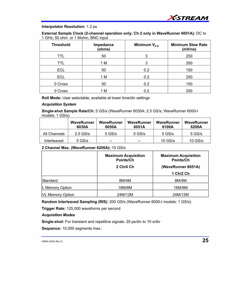
WR6A-OM-E Rev G 25
Interpolator Resolution: 1.2 ps
External Sample Clock (2-channel operation only; Ch 2 only in WaveRunner 6051A): DC to 1 GHz; 50 ohm or 1 Mohm, BNC input
Threshold Impedance (ohms)
Minimum Vp-p Minimum Slew Rate(mV/ns)
TTL 50 3 250
TTL 1 M 3 350
ECL 50 0.2 150
ECL 1 M 0.2 250
0 Cross 50 0.2 150
0 Cross 1 M 0.2 250
Roll Mode: User selectable; available at lower time/div settings Acquisition System
Single-shot Sample Rate/Ch: 5 GS/s (WaveRunner 6030A: 2.5 GS/s; WaveRunner 6000-I models: 1 GS/s)
WaveRunner 6030A
WaveRunner 6050A
WaveRunner 6051A
WaveRunner 6100A
WaveRunner 6200A
All Channels 2.5 GS/s 5 GS/s 5 GS/s 5 GS/s 5 GS/s
Interleaved 5 GS/s -- -- 10 GS/s 10 GS/s
2 Channel Max. (WaveRunner 6200A): 10 GS/s
Maximum Acquisition Points/Ch
2 Ch/4 Ch
Maximum Acquisition Points/Ch
(WaveRunner 6051A)
1 Ch/2 Ch
Standard 8M/4M 8M/4M
L Memory Option 16M/8M 16M/8M
VL Memory Option 24M/12M 24M/12M
Random Interleaved Sampling (RIS): 200 GS/s (WaveRunner 6000-I models: 1 GS/s)
Trigger Rate: 125,000 waveforms per second Acquisition Modes
Single-shot: For transient and repetitive signals: 20 ps/div to 10 s/div
Sequence: 10,000 segments max.:
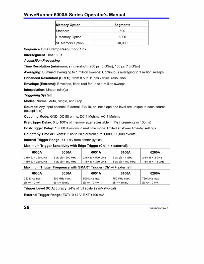
WaveRunner 6000A Series Operator's Manual
26 WR6A-OM-E Rev G
Memory Option Segments
Standard 500
L Memory Option 5000
VL Memory Option 10,000
Sequence Time Stamp Resolution: 1 ns
Intersegment Time: 8 µs Acquisition Processing
Time Resolution (minimum, single-shot): 200 ps (5 GS/s); 100 ps (10 GS/s)
Averaging: Summed averaging to 1 million sweeps; Continuous averaging to 1 million sweeps
Enhanced Resolution (ERES): from 8.5 to 11 bits vertical resolution
Envelope (Extrema): Envelope, floor, roof for up to 1 million sweeps
Interpolation: Linear, (sinx)/x Triggering System
Modes: Normal, Auto, Single, and Stop
Sources: Any input channel, External, Ext/10, or line; slope and level are unique to each source (except line)
Coupling Mode: GND, DC 50 ohms, DC 1 Mohms, AC 1 Mohms
Pre-trigger Delay: 0 to 100% of memory size (adjustable in 1% increments or 100 ns)
Post-trigger Delay: 10,000 divisions in real time mode; limited at slower time/div settings
Holdoff by Time or Events: 2 ns to 20 s or from 1 to 1,000,000,000 events
Internal Trigger Range: ±4.1 div from center (typical)
Maximum Trigger Sensitivity with Edge Trigger (Ch1-4 + external):
6030A 6050A 6051A 6100A 6200A 2 div @ < 350 MHz 1 div @ < 250 MHz
2 div @ < 500 MHz 1 div @ < 350 MHz
2 div @ < 500 MHz 1 div @ < 350 MHz
2 div @ < 1 GHz 1 div @ < 750 MHz
2 div @ < 2 GHz 1 div @ < 1.8 GHz
Maximum Trigger Frequency with SMART Trigger (Ch1-4 + external):
6030A 6050A 6051A 6100A 6200A 350 MHz max. @ >/= 10 mV
500 MHz max. @ >/= 10 mV
500 MHz max. @ >/= 10 mV
750 MHz max. @ >/= 10 mV
750 MHz max. @ >/= 10 mV
Trigger Level DC Accuracy: ±4% of full scale ±2 mV (typical)
External Trigger Range: EXT/10 ±4 V; EXT ±400 mV

WR6A-OM-E Rev G 27
Basic Triggers
Edge/Slope/Line: Triggers when the signal meets the slope and level condition. SMART Triggers
State or Edge qualified: Triggers on any input source only if a defined state or edge occurred on another input source. Delay between sources is selectable by time or events.
Dropout: Triggers if the input signal drops out for longer than a selectable time-out between 2 ns and 20 s.
Pattern: Logic combination (AND, NAND, OR, NOR) of 5 inputs (4 channels and external trigger input). Each source can be high, low, or don't care. The High and Low level can be selected independently. Triggers at start or end of pattern. SMART Triggers with Exclusion Technology
Glitch: Triggers on positive or negative glitches with widths selectable from 600 ps to 20 s or on intermittent faults (subject to bandwidth limit of scope).
Signal or Pattern Width: Triggers on positive or negative pulse widths selectable from 600 ps to 20 s or on intermittent faults (subject to bandwidth limit of scope).
Signal or Pattern Interval: Triggers on intervals selectable from 2 ns to 20 s.
Timeout (State/Edge Qualified): Triggers on any source if a given state (or transition edge) has occurred on another source
Delay between sources is 2 ns to 20 s, or 1 to 99,999,999 events
Exclusion Triggering: Trigger on intermittent faults by specifying the normal width or period. Automatic Setup
Autosetup: Automatically sets timebase, trigger, and sensitivity to display a wide range of repetitive signals.
Vertical Find Scale: Automatically sets the vertical sensitivity and offset for the selected channels to display a waveform with maximum dynamic range. Probes
Probes: One PP007-WR probe per channel standard; optional passive and active probes are available.
Caution
To avoid incorrect measurements, ensure that your PP007 probes have the correct model number (PP007-WR). Do not use probes with model number PP007-WS.
Probe System ProBus: Automatically detects and supports a wide variety of compatible probes
Scale Factors: Automatically or manually selected depending on probe used

WaveRunner 6000A Series Operator's Manual
28 WR6A-OM-E Rev G
Color Waveform Display
Type: Color 8.4-inch flat panel TFT LCD with high resolution touch screen
Resolution: SVGA; 800 x 600 pixels
Real Time Clock: Date, hours, minutes, and seconds displayed with waveform; accurate to ±50 ppm; SNTP support to synchronize to precision internet clocks
Number of Traces: Maximum of eight traces; simultaneously displays channel, zoom, memory, and math traces
Grid Styles: Single, Dual, Quad, Octal, XY, Single+XY, Dual+XY
Waveform Display Styles: Sample dots joined or dots only Analog Persistence Display
Analog and Color-graded Persistence: Variable saturation levels; stores each trace's persistence data in memory
Persistence Selections: Select analog, color, or 3-D
Trace Selection: Activate Analog Persistence on all or any combination of traces
Persistence Aging Time: From 500 ms to infinity
Sweeps Displayed: All accumulated or all accumulated with last trace highlighted Zoom Expansion Traces
Display up to 4 Math/Zoom traces Rapid Signal Processing
Processor: Intel® 2.0 GHz or better with MS Windows® XP Pro Platform
Processing Memory: 256 MB with Standard and M memory options; 512 MB with L and VL options Internal Waveform Memory
Waveform: M1, M2, M3, M4 (Store full-length waveforms with 16 bits/data point.) Or save to any number of files (limited only by data storage media). Setup Storage
Front Panel and Instrument Status: Save to the internal hard drive or to a USB-connected peripheral device. Interface
Remote Control: Through Windows Automation or LeCroy remote command set
GPIB Port (optional): Supports IEEE-488.2
Ethernet Port: 10/100Base-T Ethernet interface (RJ-45 connector)
USB Ports: 5 USB ports (one at front of scope) support Windows compatible devices.
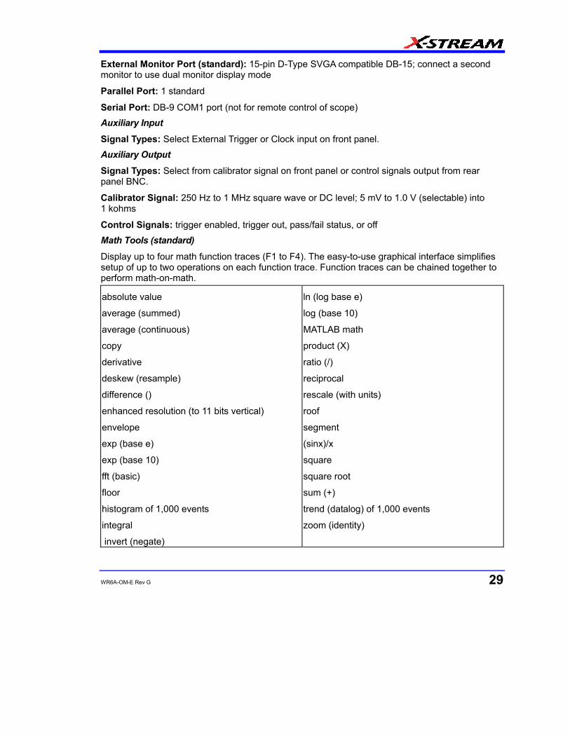
WR6A-OM-E Rev G 29
External Monitor Port (standard): 15-pin D-Type SVGA compatible DB-15; connect a second monitor to use dual monitor display mode
Parallel Port: 1 standard
Serial Port: DB-9 COM1 port (not for remote control of scope) Auxiliary Input
Signal Types: Select External Trigger or Clock input on front panel. Auxiliary Output
Signal Types: Select from calibrator signal on front panel or control signals output from rear panel BNC.
Calibrator Signal: 250 Hz to 1 MHz square wave or DC level; 5 mV to 1.0 V (selectable) into 1 kohms
Control Signals: trigger enabled, trigger out, pass/fail status, or off Math Tools (standard)
Display up to four math function traces (F1 to F4). The easy-to-use graphical interface simplifies setup of up to two operations on each function trace. Function traces can be chained together to perform math-on-math.
absolute value
average (summed)
average (continuous)
copy
derivative
deskew (resample)
difference ()
enhanced resolution (to 11 bits vertical)
envelope
exp (base e)
exp (base 10)
fft (basic)
floor
histogram of 1,000 events
integral
invert (negate)
ln (log base e)
log (base 10)
MATLAB math
product (X)
ratio (/)
reciprocal
rescale (with units)
roof
segment
(sinx)/x
square
square root
sum (+)
trend (datalog) of 1,000 events
zoom (identity)

WaveRunner 6000A Series Operator's Manual
30 WR6A-OM-E Rev G
Measure Tools (standard)
Display any 8 parameters together with statistics, including their average, high, low, and standard deviations. Histicons provide a fast, dynamic view of parameters and wave shape characteristics.
amplitude
area
base
cycles
delay
delta delay
delta time @ level
Dtrig time
duration
duty cycle
fall time (90-10%, 80-20%, @ level)
first
frequency
last
level @ x
MATLAB param
maximum
mean
minimum
number of points
overshoot+
overshoot-
peak-to-peak
period
phase
rise time (10-90%, 20-80%, @ level)
rms
std. deviation
time @ level
top
width
width negative
x @ minimum
x @ maximum
Pass/Fail Testing
Test multiple parameters against selectable parameter limits at the same time. Pass or fail conditions can initiate actions including: document to local or networked files, email the image of the failure, save waveforms, send a pulse out at the front panel auxiliary BNC output, or (with GPIB option) send a GPIB SRQ. Master Analysis Package (XMAP)
This package provides maximum capability and flexibility, and includes all the functionality present in XMATH, XDEV, and JTA2. Advanced Math Package (XMATH)
This package provides a comprehensive set of signal WaveShape Analysis tools that provide insight into the wave shape of complex signals. Additional analysis capability provided by XMAP includes:

WR6A-OM-E Rev G 31
• Parameter math -- add, subtract, multiply, or divide two different parameters.
• Histograms expanded with 19 histogram parameters and up to 2 billion events.
• Trend (datalog) of up to 1 million events
• Track graphs of any measurement parameter.
• FFT capability added to include: power averaging, power density, real and imaginary components, frequency domain parameters, and FFT on up to 25 Mpts.
• Narrow-band power measurements
• Auto-correlation function
• Sparse function
• Cubic and quadratic interpolation function Advanced Customization Package (XDEV)
This package provides a set of tools to modify the scope and customize it to meet your unique needs. Additional capability provided by XDEV includes
• Creation of your own measurement parameter or math function, using third-party software packages, and display of the result in the scope. Supported third-party software packages include: VBScript, Excel, MATLAB, Mathcad.
• CustomDSO -- create your own user interface in a scope dialog box.
• Add macro keys to run VBScript files.
• Support of plug-ins Intermediate Math Package (XWAV)
This package is a value-priced version of XMATH, with the following differences:
• Histograms can measure up to 1 million events.
• FFTs of 1 Mpts instead of full acquisition memory capacity
• No Processing Web feature
• No parameter math
• Does not include the following parameters: Nbpw, Nbphase
• Does not include the following math functions: Phistogram, Ptrace, Correlation, Track, Sparse, Interpolate
Jitter and Timing Analysis Package (JTA2)
This package provides jitter timing and analysis using JitterTrack (time), Histogram (statistical) and JitterFFT (frequency) views for common timing parameters, and other useful tools.
• Jitter and Timing parameters with JitterTrack graphs of:

WaveRunner 6000A Series Operator's Manual
32 WR6A-OM-E Rev G
Cycle-to-Cycle
N-Cycle
N-Cycle with Start selection
Frequency
Period
Half Period
Width
Time Interval Error
Setup
Hold
Skew
Duty Cycle
Duty Cycle Error (Delta Width)
• edge@lv parameter (counts edges)
• Histograms expanded with 19 histogram parameters and up to 2 billion events
• Trend (datalog) of up to one million events
• Persistence Histogram; Persistence Trace Value Analysis Package (XVAP)
This is a value-priced version of LeCroy's premier XMAP package, with the following difference: It contains XWAV and JTA2, but does not contain XDEV. Web Editor (XWEB)
The Processing Web provides a graphical way to quickly and easily set up math functions and parameter measurements. Practically unlimited math-on-math functions can be chained together, and parameter measurements for any math output waveform anywhere on the web can be inserted. Disk Drive Measurement Package (DDM2)
This package provides disk drive parameter measurements and related mathematical functions for performing disk drive WaveShape Analysis.
• Disk Drive Parameters:
amplitude symmetry
auto correlation s/n
local base
local baseline separation
local maximum
local minimum
local number
local peak-peak
local time between events
local time between peaks
local time between troughs
local time over threshold
local time trough-peak
local time under threshold
narrow band phase
narrow band power
non-linear transition shift
overwrite
pulse width 50
pulse width 50-
pulse width 50+
resolution
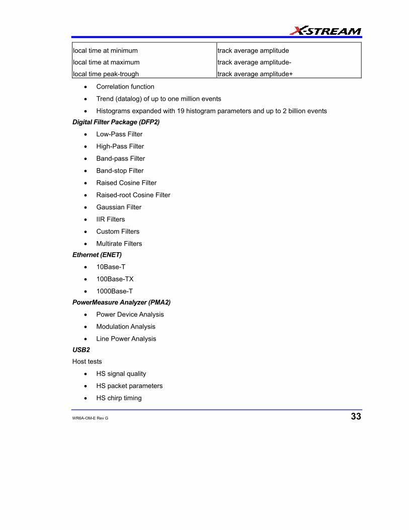
WR6A-OM-E Rev G 33
local time at minimum
local time at maximum
local time peak-trough
track average amplitude
track average amplitude-
track average amplitude+
• Correlation function
• Trend (datalog) of up to one million events
• Histograms expanded with 19 histogram parameters and up to 2 billion events Digital Filter Package (DFP2)
• Low-Pass Filter
• High-Pass Filter
• Band-pass Filter
• Band-stop Filter
• Raised Cosine Filter
• Raised-root Cosine Filter
• Gaussian Filter
• IIR Filters
• Custom Filters
• Multirate Filters Ethernet (ENET)
• 10Base-T
• 100Base-TX
• 1000Base-T PowerMeasure Analyzer (PMA2)
• Power Device Analysis
• Modulation Analysis
• Line Power Analysis USB2
Host tests
• HS signal quality
• HS packet parameters
• HS chirp timing

WaveRunner 6000A Series Operator's Manual
34 WR6A-OM-E Rev G
• HS suspend/resume/reset
• HS disconnect
• FS downstream signal quality
• LS downstream signal quality
Device tests
• HS signal quality
• HS Far-end for tethered devices
• HS Near-end for untethered devices
• HS packet parameters
• HS chirp timing
• HS suspend/resume/reset
• HS Receiver Sensitivity
• FS upstream signal quality
• LS upstream signal quality (USB 1.1 devices only)
• Inrush current.
Hub tests
• HS signal quality (Upstream/Downstream)
o HS Far-end for tethered hubs
o HS Near-end for untethered hubs
• HS packet parameters
• HS chirp timing
• HS suspend/resume/reset
• HS Receiver Sensitivity
• HS Downstream Repeater
• HS Upstream Repeater
• FS signal quality (upstream/downstream)
• LS signal quality (upstream/downstream)
• Inrush current.
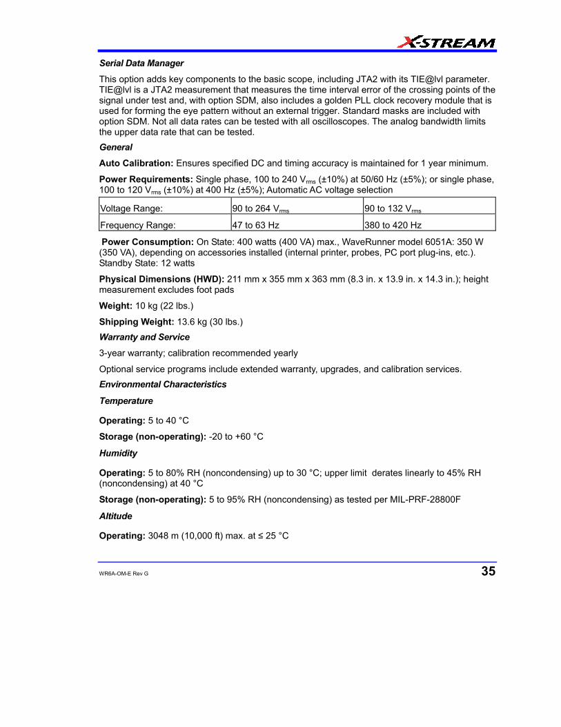
WR6A-OM-E Rev G 35
Serial Data Manager
This option adds key components to the basic scope, including JTA2 with its TIE@lvl parameter. TIE@lvl is a JTA2 measurement that measures the time interval error of the crossing points of the signal under test and, with option SDM, also includes a golden PLL clock recovery module that is used for forming the eye pattern without an external trigger. Standard masks are included with option SDM. Not all data rates can be tested with all oscilloscopes. The analog bandwidth limits the upper data rate that can be tested. General
Auto Calibration: Ensures specified DC and timing accuracy is maintained for 1 year minimum.
Power Requirements: Single phase, 100 to 240 Vrms (±10%) at 50/60 Hz (±5%); or single phase, 100 to 120 Vrms (±10%) at 400 Hz (±5%); Automatic AC voltage selection
Voltage Range: 90 to 264 Vrms 90 to 132 Vrms
Frequency Range: 47 to 63 Hz 380 to 420 Hz
Power Consumption: On State: 400 watts (400 VA) max., WaveRunner model 6051A: 350 W (350 VA), depending on accessories installed (internal printer, probes, PC port plug-ins, etc.). Standby State: 12 watts
Physical Dimensions (HWD): 211 mm x 355 mm x 363 mm (8.3 in. x 13.9 in. x 14.3 in.); height measurement excludes foot pads
Weight: 10 kg (22 lbs.)
Shipping Weight: 13.6 kg (30 lbs.) Warranty and Service
3-year warranty; calibration recommended yearly
Optional service programs include extended warranty, upgrades, and calibration services. Environmental Characteristics
Temperature
Operating: 5 to 40 °C
Storage (non-operating): -20 to +60 °C
Humidity
Operating: 5 to 80% RH (noncondensing) up to 30 °C; upper limit derates linearly to 45% RH (noncondensing) at 40 °C
Storage (non-operating): 5 to 95% RH (noncondensing) as tested per MIL-PRF-28800F
Altitude
Operating: 3048 m (10,000 ft) max. at ≤ 25 °C
WaveRunner 6000A Series Operator's Manual
36 WR6A-OM-E Rev G
Storage (non-operating): 12,192 m (40,000 ft)
Random Vibration
Operating: 5 Hz to 500 Hz, overall level: 0.31 grms, 15 minutes in each of 3 orthogonal axes
Non-operating: 5 Hz to 500 Hz, overall level: 2.4 grms, 15 minutes in each of 3 orthogonal axes
Shock
Functional Shock: 20 g peak, half sine, 11 ms pulse, 3 shocks (positive and negative) in each of 3 orthogonal axes, 18 shocks total
Certifications
Conforms to EN 61326, EN 61010-1 CE Declaration of Conformity
The oscilloscope meets requirements of EMC Directive 89/336/EEC for Electromagnetic Compatibility and Low Voltage Directive 73/23/EEC for Product Safety.
EMC Directive: EN 61326:1997 +A1:1998
EMC requirements for electrical equipment for measurement, control, and laboratory use.
EN 55011:1998 +A1:1999, Radiated and conducted emissions (Class A)*
EN 61000-3-2:2001 Harmonic Current Emissions (Class A)
Electromagnetic Emissions:
EN 61000-3-3:1995 +A1:2001 Voltage Fluctuations and Flickers (Pst = 1)
* To conform to Radiated Emissions standard, use properly shielded cables on all I/O terminals.
Warning
This is a Class A product. In a domestic environment this product may cause radio interference, in which case the user may be required to take appropriate measures.
EN 61000-4-2:1995 +A2:2001* Electrostatic Discharge
(4 kV contact, 8 kV air, 4 kV vertical/horizontal coupling planes)
EN 61000-4-3:2002* RF Radiated Electromagnetic Field
(3 V/m, 80-1000 MHz)
EN 61000-4-4:1995 +A2:2001* Electrical Fast Transient/Burst
(1 kV AC Mains, 0.5 kV I/O signal/control)
Electromagnetic Immunity:
EN 61000-4-5:1995 +A1:2001* Surges
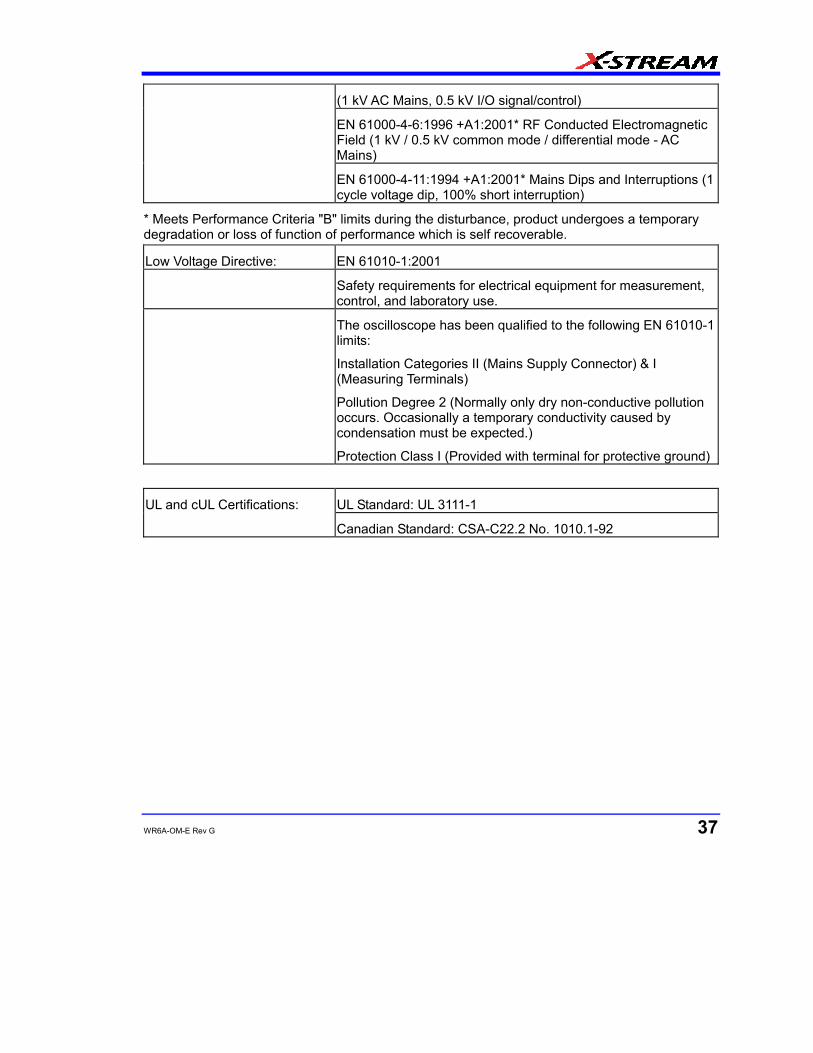
WR6A-OM-E Rev G 37
(1 kV AC Mains, 0.5 kV I/O signal/control)
EN 61000-4-6:1996 +A1:2001* RF Conducted Electromagnetic Field (1 kV / 0.5 kV common mode / differential mode - AC Mains)
EN 61000-4-11:1994 +A1:2001* Mains Dips and Interruptions (1 cycle voltage dip, 100% short interruption)
* Meets Performance Criteria "B" limits during the disturbance, product undergoes a temporary degradation or loss of function of performance which is self recoverable.
Low Voltage Directive: EN 61010-1:2001
Safety requirements for electrical equipment for measurement, control, and laboratory use.
The oscilloscope has been qualified to the following EN 61010-1 limits:
Installation Categories II (Mains Supply Connector) & I (Measuring Terminals)
Pollution Degree 2 (Normally only dry non-conductive pollution occurs. Occasionally a temporary conductivity caused by condensation must be expected.)
Protection Class I (Provided with terminal for protective ground)
UL Standard: UL 3111-1 UL and cUL Certifications:
Canadian Standard: CSA-C22.2 No. 1010.1-92

WaveRunner 6000A Series Operator's Manual
38 WR6A-OM-E Rev G
China RoHS Compliance
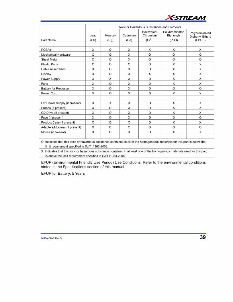
WR6A-OM-E Rev G 39
Toxic or Hazardous Substances and Elements
Part Name Lead (Pb)
Mercury (Hg)
Cadmium (Cd)
Hexavalent Chromium
(Cr6+)
Polybrominated Biphenyls
(PBB)
Polybrominated Diphenyl Ethers
(PBDE) PCBAs X O X X X X Mechanical Hardware O O X O O O Sheet Metal O O X O O O Plastic Parts O O O O X X Cable Assemblies X O X O X X Display X O X X X X Power Supply X X X O X X Fans X O X O X X Battery for Processor X O X O O O Power Cord X O X O X X Ext Power Supply (if present) X X X O X X Probes (if present) X O X O X X CD Drive (if present) X O X O X X Fuse (if present) X O X O O O Product Case (if present) O O O O X X Adapters/Modules (if present) X O O O O O Mouse (if present) X O X O X X O: Indicates that this toxic or hazardous substance contained in all of the homogeneous materials for this part is below the limit requirement specified in SJ/T11363-2006. X: Indicates that this toxic or hazardous substance contained in at least one of the homogenous materials used for this part is above the limit requirement specified in SJ/T11363-2006.
EFUP (Environmental Friendly Use Period) Use Conditions: Refer to the environmental conditions stated in the Specifications section of this manual.
EFUP for Battery: 5 Years
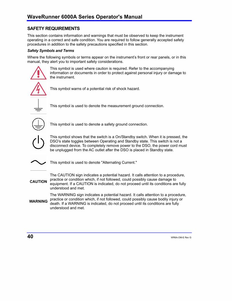
WaveRunner 6000A Series Operator's Manual
40 WR6A-OM-E Rev G
SAFETY REQUIREMENTS This section contains information and warnings that must be observed to keep the instrument operating in a correct and safe condition. You are required to follow generally accepted safety procedures in addition to the safety precautions specified in this section. Safety Symbols and Terms
Where the following symbols or terms appear on the instrument’s front or rear panels, or in this manual, they alert you to important safety considerations.
This symbol is used where caution is required. Refer to the accompanying information or documents in order to protect against personal injury or damage to the instrument.
This symbol warns of a potential risk of shock hazard.
This symbol is used to denote the measurement ground connection.
This symbol is used to denote a safety ground connection.
This symbol shows that the switch is a On/Standby switch. When it is pressed, the DSO’s state toggles between Operating and Standby state. This switch is not a disconnect device. To completely remove power to the DSO, the power cord must be unplugged from the AC outlet after the DSO is placed in Standby state.
This symbol is used to denote "Alternating Current."
CAUTION
The CAUTION sign indicates a potential hazard. It calls attention to a procedure, practice or condition which, if not followed, could possibly cause damage to equipment. If a CAUTION is indicated, do not proceed until its conditions are fully understood and met.
WARNING
The WARNING sign indicates a potential hazard. It calls attention to a procedure, practice or condition which, if not followed, could possibly cause bodily injury or death. If a WARNING is indicated, do not proceed until its conditions are fully understood and met.
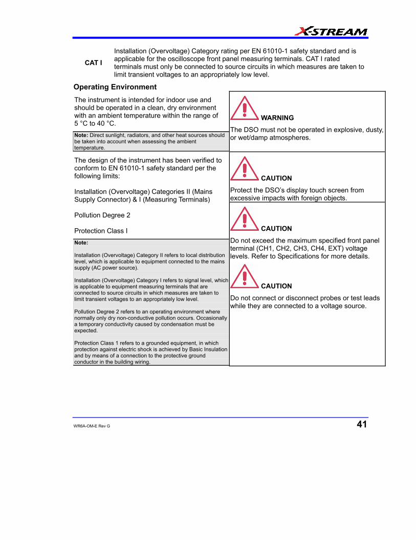
WR6A-OM-E Rev G 41
CAT I Installation (Overvoltage) Category rating per EN 61010-1 safety standard and is applicable for the oscilloscope front panel measuring terminals. CAT I rated terminals must only be connected to source circuits in which measures are taken to limit transient voltages to an appropriately low level.
Operating Environment The instrument is intended for indoor use and should be operated in a clean, dry environment with an ambient temperature within the range of 5 °C to 40 °C. Note: Direct sunlight, radiators, and other heat sources should be taken into account when assessing the ambient temperature.
WARNING
The DSO must not be operated in explosive, dusty, or wet/damp atmospheres.
CAUTION
Protect the DSO’s display touch screen from excessive impacts with foreign objects.
The design of the instrument has been verified to conform to EN 61010-1 safety standard per the following limits: Installation (Overvoltage) Categories II (Mains Supply Connector) & I (Measuring Terminals) Pollution Degree 2 Protection Class I Note: Installation (Overvoltage) Category II refers to local distribution level, which is applicable to equipment connected to the mains supply (AC power source). Installation (Overvoltage) Category I refers to signal level, which is applicable to equipment measuring terminals that are connected to source circuits in which measures are taken to limit transient voltages to an appropriately low level. Pollution Degree 2 refers to an operating environment where normally only dry non-conductive pollution occurs. Occasionally a temporary conductivity caused by condensation must be expected. Protection Class 1 refers to a grounded equipment, in which protection against electric shock is achieved by Basic Insulation and by means of a connection to the protective ground conductor in the building wiring.
CAUTION
Do not exceed the maximum specified front panel terminal (CH1, CH2, CH3, CH4, EXT) voltage levels. Refer to Specifications for more details.
CAUTION
Do not connect or disconnect probes or test leads while they are connected to a voltage source.
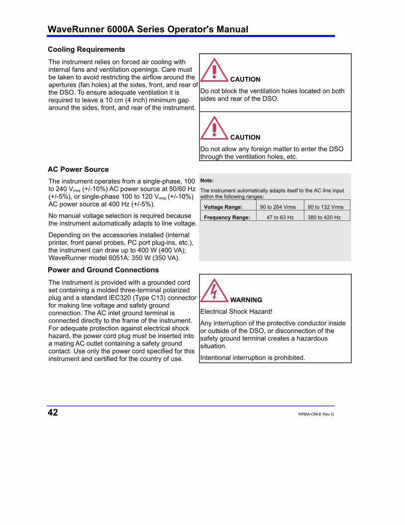
WaveRunner 6000A Series Operator's Manual
42 WR6A-OM-E Rev G
Cooling Requirements The instrument relies on forced air cooling with internal fans and ventilation openings. Care must be taken to avoid restricting the airflow around the apertures (fan holes) at the sides, front, and rear of the DSO. To ensure adequate ventilation it is required to leave a 10 cm (4 inch) minimum gap around the sides, front, and rear of the instrument.
CAUTION
Do not block the ventilation holes located on both sides and rear of the DSO.
CAUTION
Do not allow any foreign matter to enter the DSO through the ventilation holes, etc.
AC Power Source The instrument operates from a single-phase, 100 to 240 Vrms (+/-10%) AC power source at 50/60 Hz (+/-5%), or single-phase 100 to 120 Vrms (+/-10%) AC power source at 400 Hz (+/-5%).
No manual voltage selection is required because the instrument automatically adapts to line voltage.
Depending on the accessories installed (internal printer, front panel probes, PC port plug-ins, etc.), the instrument can draw up to 400 W (400 VA); WaveRunner model 6051A: 350 W (350 VA).
Note:
The instrument automatically adapts itself to the AC line input within the following ranges:
Voltage Range: 90 to 264 Vrms 90 to 132 Vrms
Frequency Range: 47 to 63 Hz 380 to 420 Hz
Power and Ground Connections The instrument is provided with a grounded cord set containing a molded three-terminal polarized plug and a standard IEC320 (Type C13) connector for making line voltage and safety ground connection. The AC inlet ground terminal is connected directly to the frame of the instrument. For adequate protection against electrical shock hazard, the power cord plug must be inserted into a mating AC outlet containing a safety ground contact. Use only the power cord specified for this instrument and certified for the country of use.
WARNING
Electrical Shock Hazard!
Any interruption of the protective conductor inside or outside of the DSO, or disconnection of the safety ground terminal creates a hazardous situation.
Intentional interruption is prohibited.
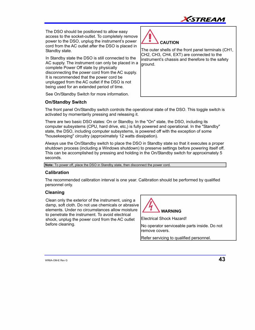
WR6A-OM-E Rev G 43
The DSO should be positioned to allow easy access to the socket-outlet. To completely remove power to the DSO, unplug the instrument’s power cord from the AC outlet after the DSO is placed in Standby state.
In Standby state the DSO is still connected to the AC supply. The instrument can only be placed in a complete Power Off state by physically disconnecting the power cord from the AC supply. It is recommended that the power cord be unplugged from the AC outlet if the DSO is not being used for an extended period of time.
See On/Standby Switch for more information.
CAUTION
The outer shells of the front panel terminals (CH1, CH2, CH3, CH4, EXT) are connected to the instrument’s chassis and therefore to the safety ground.
On/Standby Switch The front panel On/Standby switch controls the operational state of the DSO. This toggle switch is activated by momentarily pressing and releasing it.
There are two basic DSO states: On or Standby. In the "On" state, the DSO, including its computer subsystems (CPU, hard drive, etc,) is fully powered and operational. In the "Standby" state, the DSO, including computer subsystems, is powered off with the exception of some "housekeeping" circuitry (approximately 12 watts dissipation).
Always use the On/Standby switch to place the DSO in Standby state so that it executes a proper shutdown process (including a Windows shutdown) to preserve settings before powering itself off. This can be accomplished by pressing and holding in the On/Standby switch for approximately 5 seconds.
Note: To power off, place the DSO in Standby state, then disconnect the power cord.
Calibration The recommended calibration interval is one year. Calibration should be performed by qualified personnel only.
Cleaning Clean only the exterior of the instrument, using a damp, soft cloth. Do not use chemicals or abrasive elements. Under no circumstances allow moisture to penetrate the instrument. To avoid electrical shock, unplug the power cord from the AC outlet before cleaning.
WARNING
Electrical Shock Hazard!
No operator serviceable parts inside. Do not remove covers.
Refer servicing to qualified personnel.
WaveRunner 6000A Series Operator's Manual
44 WR6A-OM-E Rev G
Abnormal Conditions Operate the instrument only as intended by the manufacturer.
If you suspect the DSO’s protection has been impaired, disconnect the power cord and secure the instrument against any unintended operation.
The DSO’s protection is likely to be impaired if, for example, the instrument shows visible damage or has been subjected to severe transport stresses.
Proper use of the instrument depends on careful reading of all instructions and labels.
WARNING
Any use of the DSO in a manner not specified by the manufacturer may impair the instrument’s safety protection. The instrument and related accessories should not be directly connected to human subjects or used for patient monitoring.
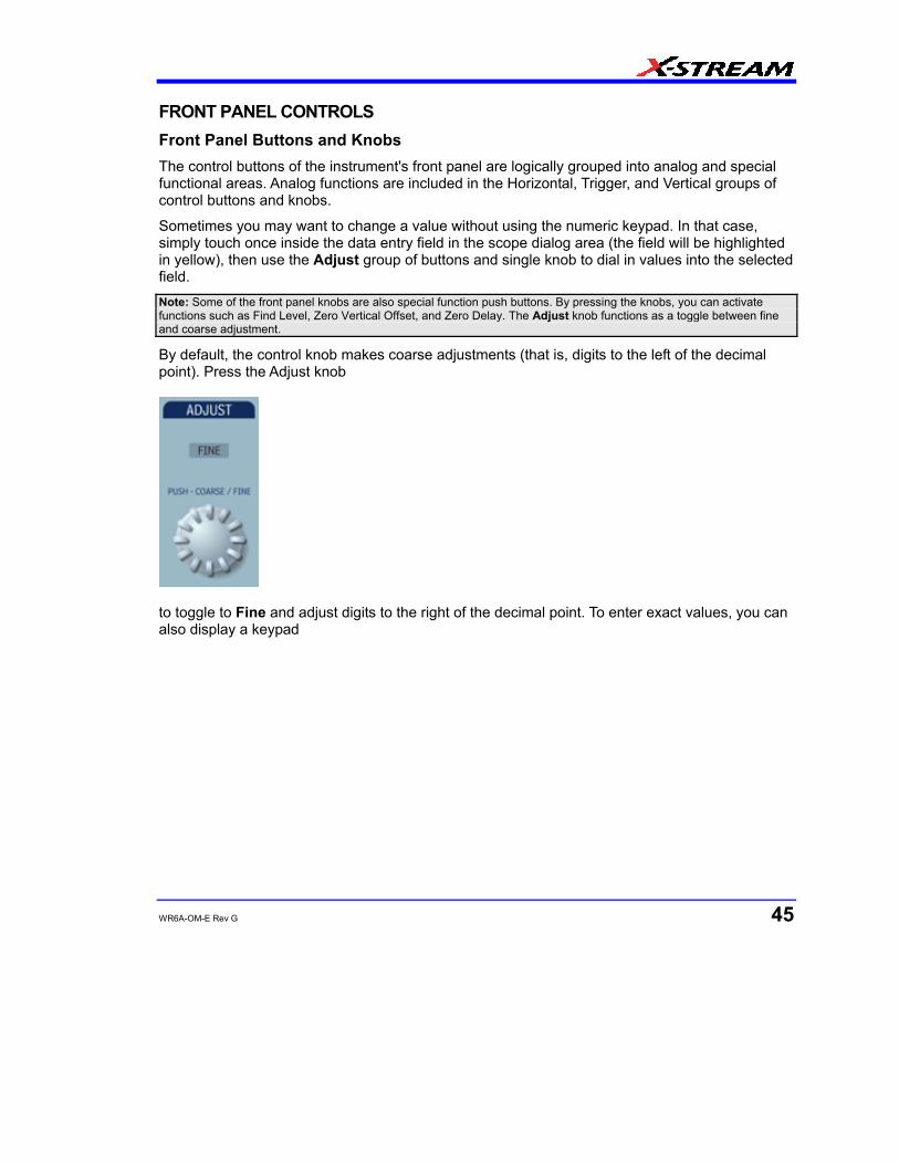
WR6A-OM-E Rev G 45
FRONT PANEL CONTROLS Front Panel Buttons and Knobs The control buttons of the instrument's front panel are logically grouped into analog and special functional areas. Analog functions are included in the Horizontal, Trigger, and Vertical groups of control buttons and knobs.
Sometimes you may want to change a value without using the numeric keypad. In that case, simply touch once inside the data entry field in the scope dialog area (the field will be highlighted in yellow), then use the Adjust group of buttons and single knob to dial in values into the selected field. Note: Some of the front panel knobs are also special function push buttons. By pressing the knobs, you can activate functions such as Find Level, Zero Vertical Offset, and Zero Delay. The Adjust knob functions as a toggle between fine and coarse adjustment.
By default, the control knob makes coarse adjustments (that is, digits to the left of the decimal point). Press the Adjust knob
to toggle to Fine and adjust digits to the right of the decimal point. To enter exact values, you can also display a keypad
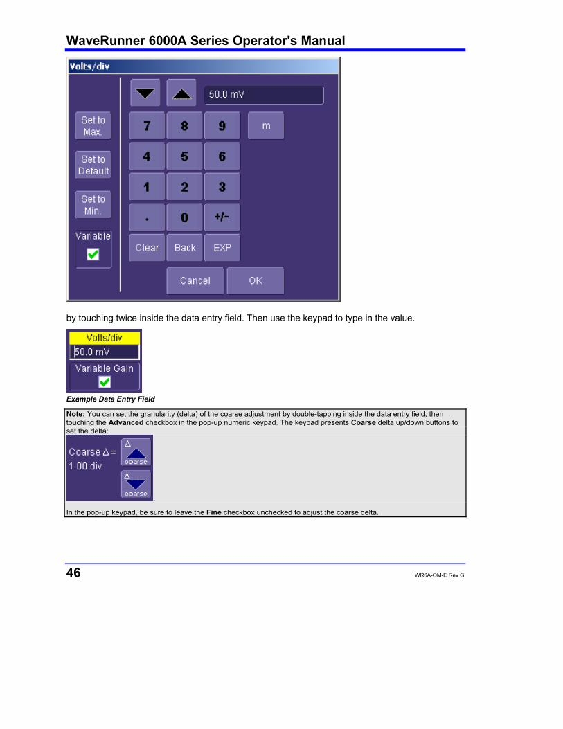
WaveRunner 6000A Series Operator's Manual
46 WR6A-OM-E Rev G
by touching twice inside the data entry field. Then use the keypad to type in the value.
Example Data Entry Field Note: You can set the granularity (delta) of the coarse adjustment by double-tapping inside the data entry field, then touching the Advanced checkbox in the pop-up numeric keypad. The keypad presents Coarse delta up/down buttons to set the delta:
.
In the pop-up keypad, be sure to leave the Fine checkbox unchecked to adjust the coarse delta.

WR6A-OM-E Rev G 47
Trigger Knobs:
Level Selects the trigger threshold level. Press this knob to quickly set the level to
zero. The Level is indicated in the Trigger descriptor label .
Trigger Buttons:
Stop Prevents the scope from triggering on a signal. If you boot up the instrument with the trigger in Stop mode, the message "no trace available" will be displayed. Press Auto to display your trace.
Auto Triggers the scope after a time-out, even if the trigger conditions are not met.
Normal Triggers the scope each time a signal is present that meets the conditions set for the type of trigger selected.
Single Arms the scope to trigger once (single-shot acquisition) when the input signal meets the trigger conditions set for the type of trigger selected. If the scope is already armed, it will force a trigger.
Horizontal Knobs:
Delay Horizontally positions the scope trace on the display so you can observe the signal prior to the trigger time. Delay adjusts the pre- and post-trigger time. Press this knob to quickly set the delay to zero. The trigger point is positioned in the middle of the display grid.
Time/Division Sets the time/division of the scope timebase (acquisition system).
Vertical Knobs:
Offset Adjusts the vertical offset of a channel. Press these knobs to quickly set the offset to zero.
Volts/Div Adjusts the Volts/Division setting (vertical gain) of the channel selected.
Channel Buttons:
1, 2, 3, 4 Turns a channel on or off. These buttons activate the dialog that lets you change the channel's setup conditions including coupling, gain, and offset. They are used also to select multiple grids, to automatically set the gain (FIND SCALE), or to automatically display a zoom of the signal. Press twice to toggle the trace on and off.
WaveRunner 6000A Series Operator's Manual
48 WR6A-OM-E Rev G
Wavepilot Control Knobs:
Position Adjusts the horizontal position of a zoom trace on the display. The zoom region is highlighted in color on the source trace.
Zoom Adjusts the horizontal zoom (magnification factor) of the selected zoom trace.
Position Adjusts the vertical position of the selected zoom trace on the display.
Zoom Adjusts the vertical zoom (magnification factor) of the selected zoom trace on the display.
Special Features Buttons:
Auto Setup Automatically sets the scope's horizontal timebase (acquisition system), vertical gain and offset, as well as trigger conditions, to display a wide variety of signals.
Analog Persist
Provides a three dimensional view of the signal: time, voltage, and a third dimension related to the frequency of occurrence, as shown by a color-graded (thermal) or intensity-graded display.
General Control Buttons:
Print Screen
Prints the displayed screen to a file, a printer, the clipboard, or attaches it as an e-mail. Select the device and format it in the Utilities Hardcopy dialog.
Touch Screen (toggle switch)
Activates or deactivates the touch screen.
Clear Sweeps Clears data from multiple sweeps (acquisitions) including: persistence trace displays, averaged traces, parameter statistics, and Histicons. During waveform readout, cancels readout.
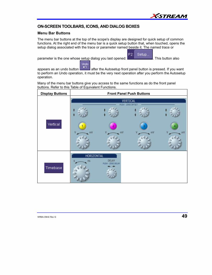
WR6A-OM-E Rev G 49
ON-SCREEN TOOLBARS, ICONS, AND DIALOG BOXES Menu Bar Buttons The menu bar buttons at the top of the scope's display are designed for quick setup of common functions. At the right end of the menu bar is a quick setup button that, when touched, opens the setup dialog associated with the trace or parameter named beside it. The named trace or
parameter is the one whose setup dialog you last opened: . This button also
appears as an undo button after the Autosetup front panel button is pressed. If you want to perform an Undo operation, it must be the very next operation after you perform the Autosetup operation.
Many of the menu bar buttons give you access to the same functions as do the front panel buttons. Refer to this Table of Equivalent Functions.
Display Buttons Front Panel Push Buttons
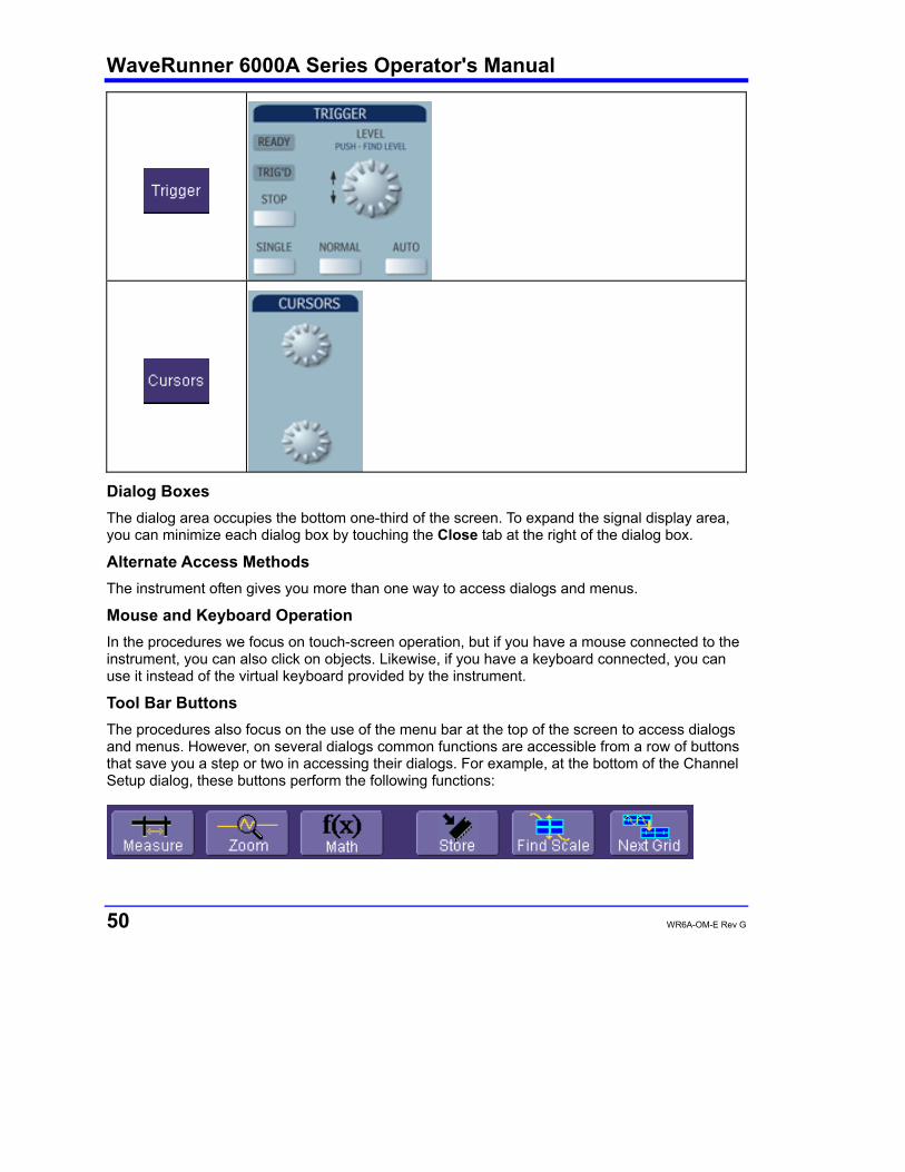
WaveRunner 6000A Series Operator's Manual
50 WR6A-OM-E Rev G
Dialog Boxes The dialog area occupies the bottom one-third of the screen. To expand the signal display area, you can minimize each dialog box by touching the Close tab at the right of the dialog box.
Alternate Access Methods The instrument often gives you more than one way to access dialogs and menus.
Mouse and Keyboard Operation In the procedures we focus on touch-screen operation, but if you have a mouse connected to the instrument, you can also click on objects. Likewise, if you have a keyboard connected, you can use it instead of the virtual keyboard provided by the instrument.
Tool Bar Buttons The procedures also focus on the use of the menu bar at the top of the screen to access dialogs and menus. However, on several dialogs common functions are accessible from a row of buttons that save you a step or two in accessing their dialogs. For example, at the bottom of the Channel Setup dialog, these buttons perform the following functions:
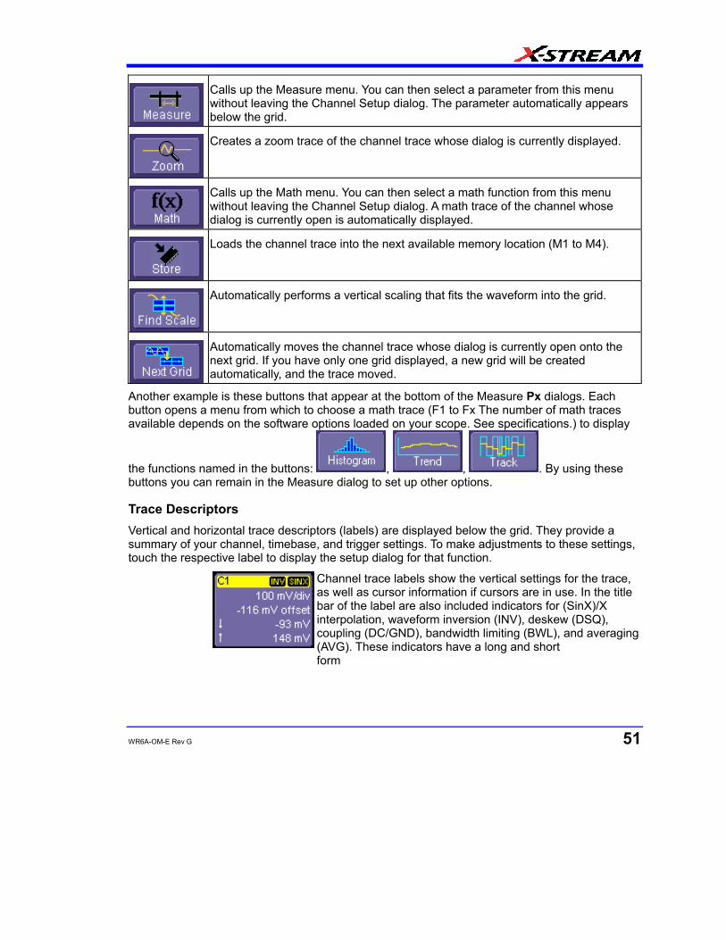
WR6A-OM-E Rev G 51
Calls up the Measure menu. You can then select a parameter from this menu without leaving the Channel Setup dialog. The parameter automatically appears below the grid.
Creates a zoom trace of the channel trace whose dialog is currently displayed.
Calls up the Math menu. You can then select a math function from this menu without leaving the Channel Setup dialog. A math trace of the channel whose dialog is currently open is automatically displayed.
Loads the channel trace into the next available memory location (M1 to M4).
Automatically performs a vertical scaling that fits the waveform into the grid.
Automatically moves the channel trace whose dialog is currently open onto the next grid. If you have only one grid displayed, a new grid will be created automatically, and the trace moved.
Another example is these buttons that appear at the bottom of the Measure Px dialogs. Each button opens a menu from which to choose a math trace (F1 to Fx The number of math traces available depends on the software options loaded on your scope. See specifications.) to display
the functions named in the buttons: , , . By using these buttons you can remain in the Measure dialog to set up other options.
Trace Descriptors Vertical and horizontal trace descriptors (labels) are displayed below the grid. They provide a summary of your channel, timebase, and trigger settings. To make adjustments to these settings, touch the respective label to display the setup dialog for that function.
Channel trace labels show the vertical settings for the trace, as well as cursor information if cursors are in use. In the title bar of the label are also included indicators for (SinX)/X interpolation, waveform inversion (INV), deskew (DSQ), coupling (DC/GND), bandwidth limiting (BWL), and averaging (AVG). These indicators have a long and short form
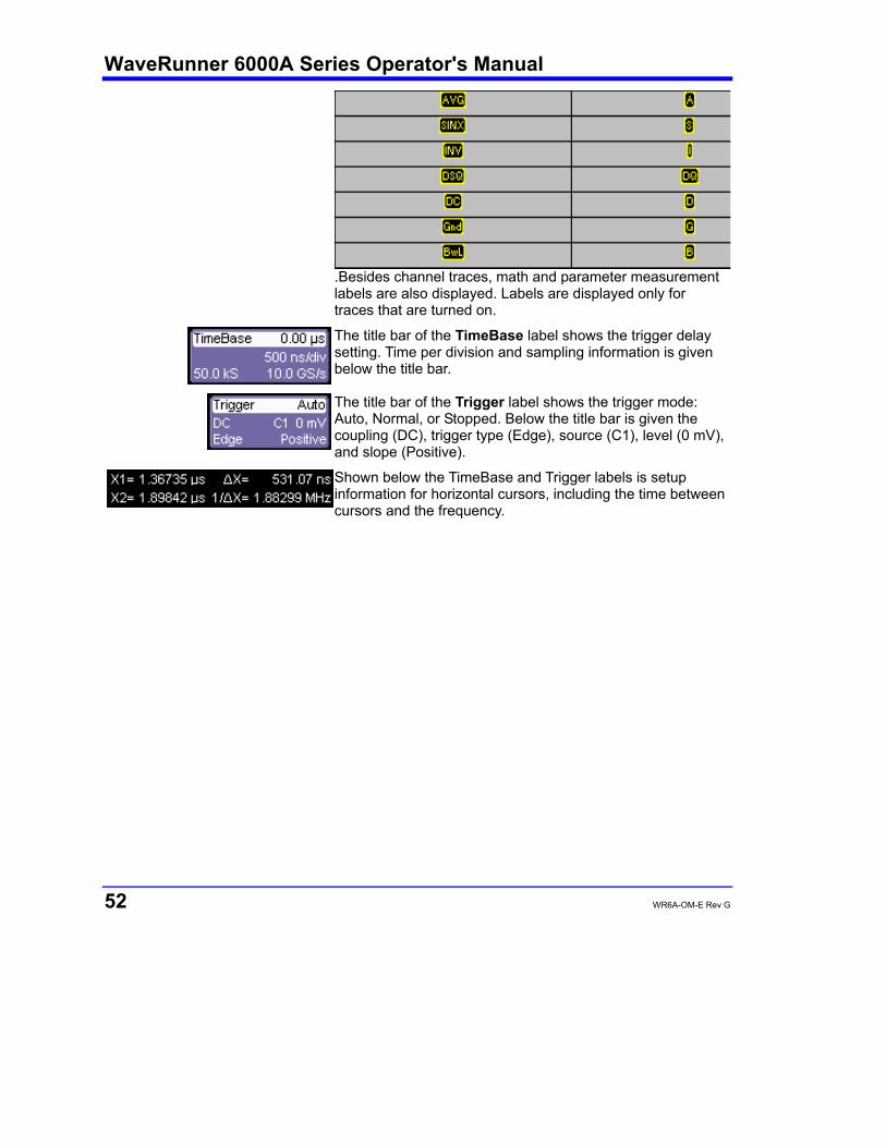
WaveRunner 6000A Series Operator's Manual
52 WR6A-OM-E Rev G
.Besides channel traces, math and parameter measurement labels are also displayed. Labels are displayed only for traces that are turned on.
The title bar of the TimeBase label shows the trigger delay setting. Time per division and sampling information is given below the title bar.
The title bar of the Trigger label shows the trigger mode: Auto, Normal, or Stopped. Below the title bar is given the coupling (DC), trigger type (Edge), source (C1), level (0 mV), and slope (Positive).
Shown below the TimeBase and Trigger labels is setup information for horizontal cursors, including the time between cursors and the frequency.
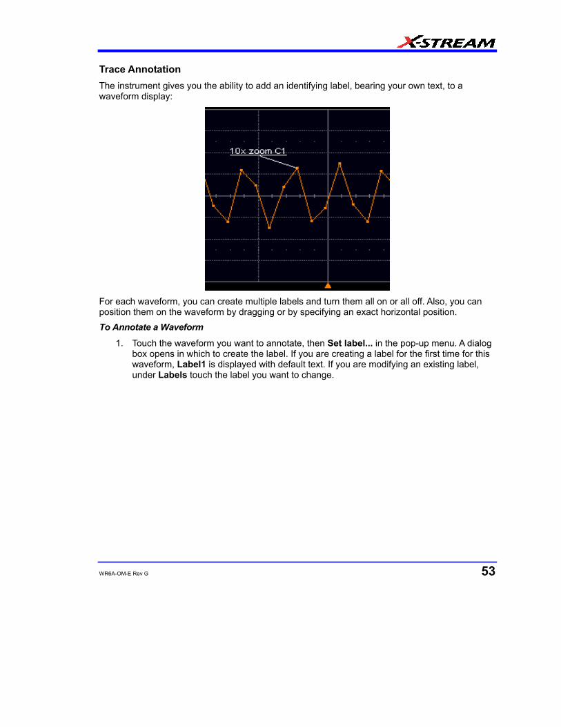
WR6A-OM-E Rev G 53
Trace Annotation The instrument gives you the ability to add an identifying label, bearing your own text, to a waveform display:
For each waveform, you can create multiple labels and turn them all on or all off. Also, you can position them on the waveform by dragging or by specifying an exact horizontal position. To Annotate a Waveform
1. Touch the waveform you want to annotate, then Set label... in the pop-up menu. A dialog box opens in which to create the label. If you are creating a label for the first time for this waveform, Label1 is displayed with default text. If you are modifying an existing label, under Labels touch the label you want to change.
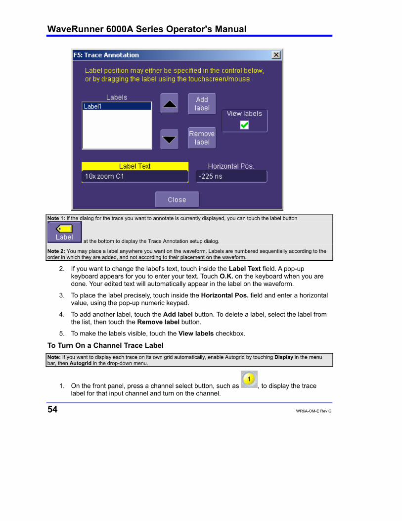
WaveRunner 6000A Series Operator's Manual
54 WR6A-OM-E Rev G
Note 1: If the dialog for the trace you want to annotate is currently displayed, you can touch the label button
at the bottom to display the Trace Annotation setup dialog.
Note 2: You may place a label anywhere you want on the waveform. Labels are numbered sequentially according to the order in which they are added, and not according to their placement on the waveform.
2. If you want to change the label's text, touch inside the Label Text field. A pop-up keyboard appears for you to enter your text. Touch O.K. on the keyboard when you are done. Your edited text will automatically appear in the label on the waveform.
3. To place the label precisely, touch inside the Horizontal Pos. field and enter a horizontal value, using the pop-up numeric keypad.
4. To add another label, touch the Add label button. To delete a label, select the label from the list, then touch the Remove label button.
5. To make the labels visible, touch the View labels checkbox.
To Turn On a Channel Trace Label Note: If you want to display each trace on its own grid automatically, enable Autogrid by touching Display in the menu bar, then Autogrid in the drop-down menu.
1. On the front panel, press a channel select button, such as , to display the trace label for that input channel and turn on the channel.
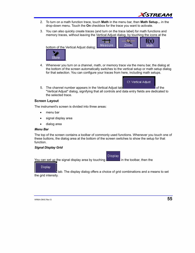
WR6A-OM-E Rev G 55
2. To turn on a math function trace, touch Math in the menu bar, then Math Setup... in the drop-down menu. Touch the On checkbox for the trace you want to activate.
3. You can also quickly create traces (and turn on the trace label) for math functions and memory traces, without leaving the Vertical Adjust dialog, by touching the icons at the
bottom of the Vertical Adjust dialog: , , ,
.
4. Whenever you turn on a channel, math, or memory trace via the menu bar, the dialog at the bottom of the screen automatically switches to the vertical setup or math setup dialog for that selection. You can configure your traces from here, including math setups.
5. The channel number appears in the Vertical Adjust tab of the "Vertical Adjust" dialog, signifying that all controls and data entry fields are dedicated to the selected trace.
Screen Layout The instrument's screen is divided into three areas:
• menu bar
• signal display area
• dialog area Menu Bar
The top of the screen contains a toolbar of commonly used functions. Whenever you touch one of these buttons, the dialog area at the bottom of the screen switches to show the setup for that function. Signal Display Grid
You can set up the signal display area by touching in the toolbar, then the
tab. The display dialog offers a choice of grid combinations and a means to set the grid intensity.
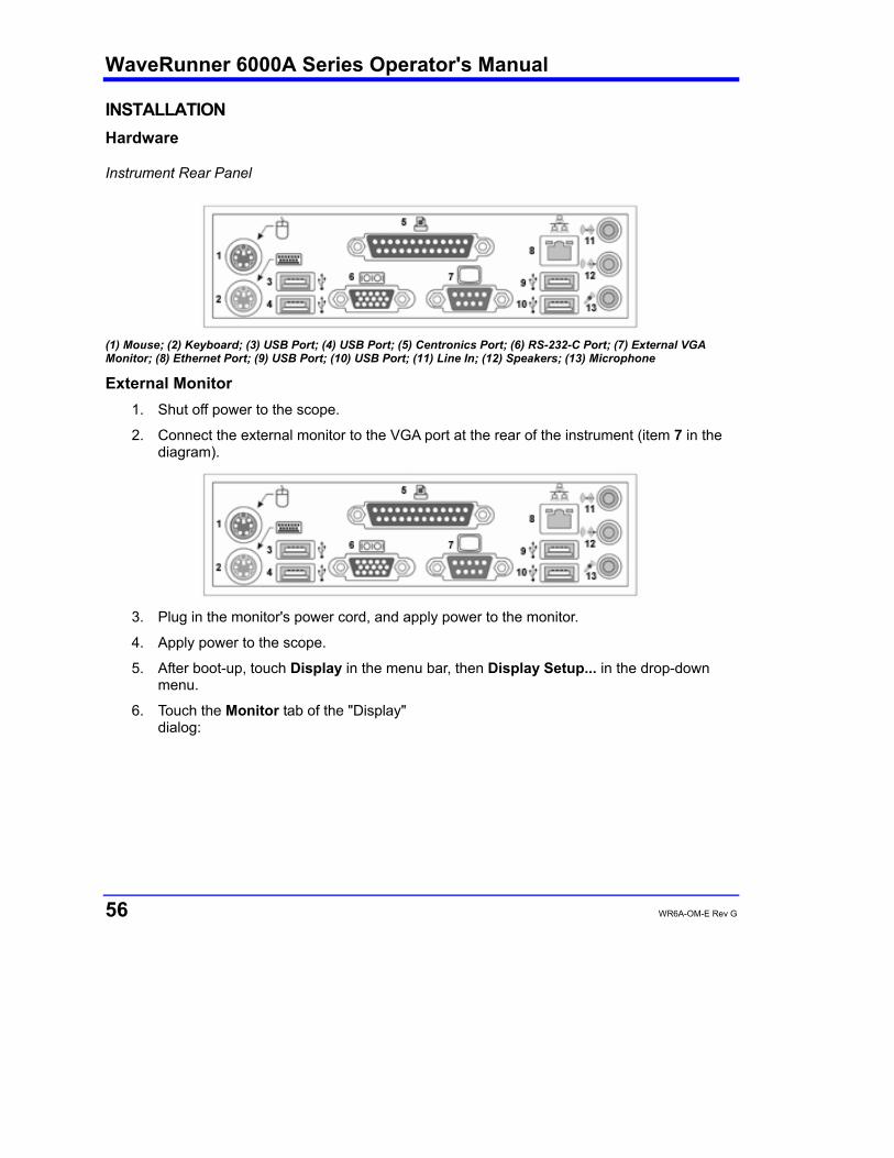
WaveRunner 6000A Series Operator's Manual
56 WR6A-OM-E Rev G
INSTALLATION Hardware
Instrument Rear Panel
(1) Mouse; (2) Keyboard; (3) USB Port; (4) USB Port; (5) Centronics Port; (6) RS-232-C Port; (7) External VGA Monitor; (8) Ethernet Port; (9) USB Port; (10) USB Port; (11) Line In; (12) Speakers; (13) Microphone External Monitor
1. Shut off power to the scope.
2. Connect the external monitor to the VGA port at the rear of the instrument (item 7 in the diagram).
3. Plug in the monitor's power cord, and apply power to the monitor.
4. Apply power to the scope.
5. After boot-up, touch Display in the menu bar, then Display Setup... in the drop-down menu.
6. Touch the Monitor tab of the "Display" dialog:
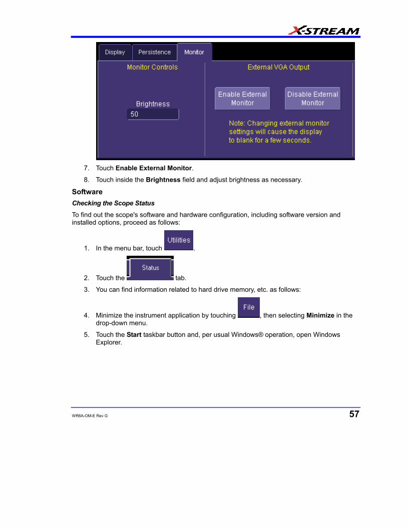
WR6A-OM-E Rev G 57
7. Touch Enable External Monitor.
8. Touch inside the Brightness field and adjust brightness as necessary.
Software Checking the Scope Status
To find out the scope's software and hardware configuration, including software version and installed options, proceed as follows:
1. In the menu bar, touch .
2. Touch the tab.
3. You can find information related to hard drive memory, etc. as follows:
4. Minimize the instrument application by touching , then selecting Minimize in the drop-down menu.
5. Touch the Start taskbar button and, per usual Windows® operation, open Windows Explorer.
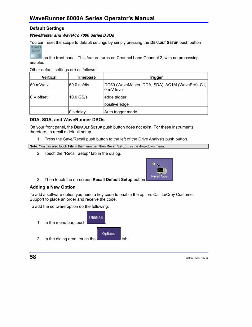
WaveRunner 6000A Series Operator's Manual
58 WR6A-OM-E Rev G
Default Settings WaveMaster and WavePro 7000 Series DSOs
You can reset the scope to default settings by simply pressing the DEFAULT SETUP push button
on the front panel. This feature turns on Channel1 and Channel 2, with no processing enabled.
Other default settings are as follows:
Vertical Timebase Trigger
50 mV/div 50.0 ns/div DC50 (WaveMaster, DDA, SDA), AC1M (WavePro), C1, 0 mV level
0 V offset 10.0 GS/s edge trigger
positive edge
0 s delay Auto trigger mode
DDA, SDA, and WaveRunner DSOs On your front panel, the DEFAULT SETUP push button does not exist. For these instruments, therefore, to recall a default setup
1. Press the Save/Recall push button to the left of the Drive Analysis push button.
Note: You can also touch File in the menu bar, then Recall Setup... in the drop-down menu.
2. Touch the "Recall Setup" tab in the dialog.
3. Then touch the on-screen Recall Default Setup button .
Adding a New Option To add a software option you need a key code to enable the option. Call LeCroy Customer Support to place an order and receive the code.
To add the software option do the following:
1. In the menu bar, touch .
2. In the dialog area, touch the tab.
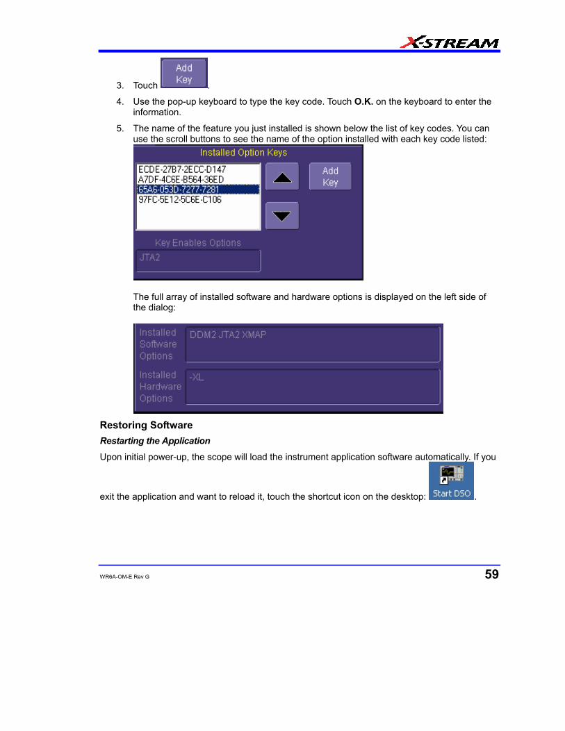
WR6A-OM-E Rev G 59
3. Touch .
4. Use the pop-up keyboard to type the key code. Touch O.K. on the keyboard to enter the information.
5. The name of the feature you just installed is shown below the list of key codes. You can use the scroll buttons to see the name of the option installed with each key code listed:
The full array of installed software and hardware options is displayed on the left side of the dialog:
Restoring Software Restarting the Application
Upon initial power-up, the scope will load the instrument application software automatically. If you
exit the application and want to reload it, touch the shortcut icon on the desktop: .
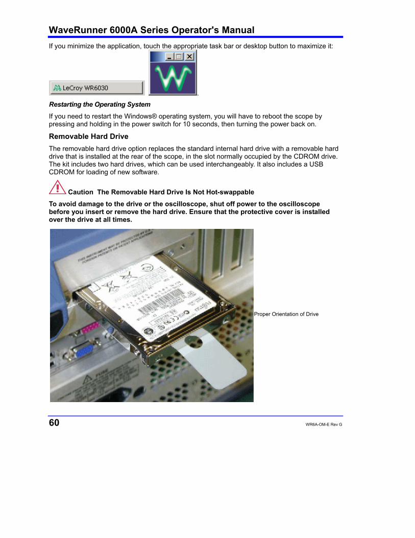
WaveRunner 6000A Series Operator's Manual
60 WR6A-OM-E Rev G
If you minimize the application, touch the appropriate task bar or desktop button to maximize it:
. Restarting the Operating System
If you need to restart the Windows® operating system, you will have to reboot the scope by pressing and holding in the power switch for 10 seconds, then turning the power back on.
Removable Hard Drive The removable hard drive option replaces the standard internal hard drive with a removable hard drive that is installed at the rear of the scope, in the slot normally occupied by the CDROM drive. The kit includes two hard drives, which can be used interchangeably. It also includes a USB CDROM for loading of new software.
Caution The Removable Hard Drive Is Not Hot-swappable
To avoid damage to the drive or the oscilloscope, shut off power to the oscilloscope before you insert or remove the hard drive. Ensure that the protective cover is installed over the drive at all times.
Proper Orientation of Drive
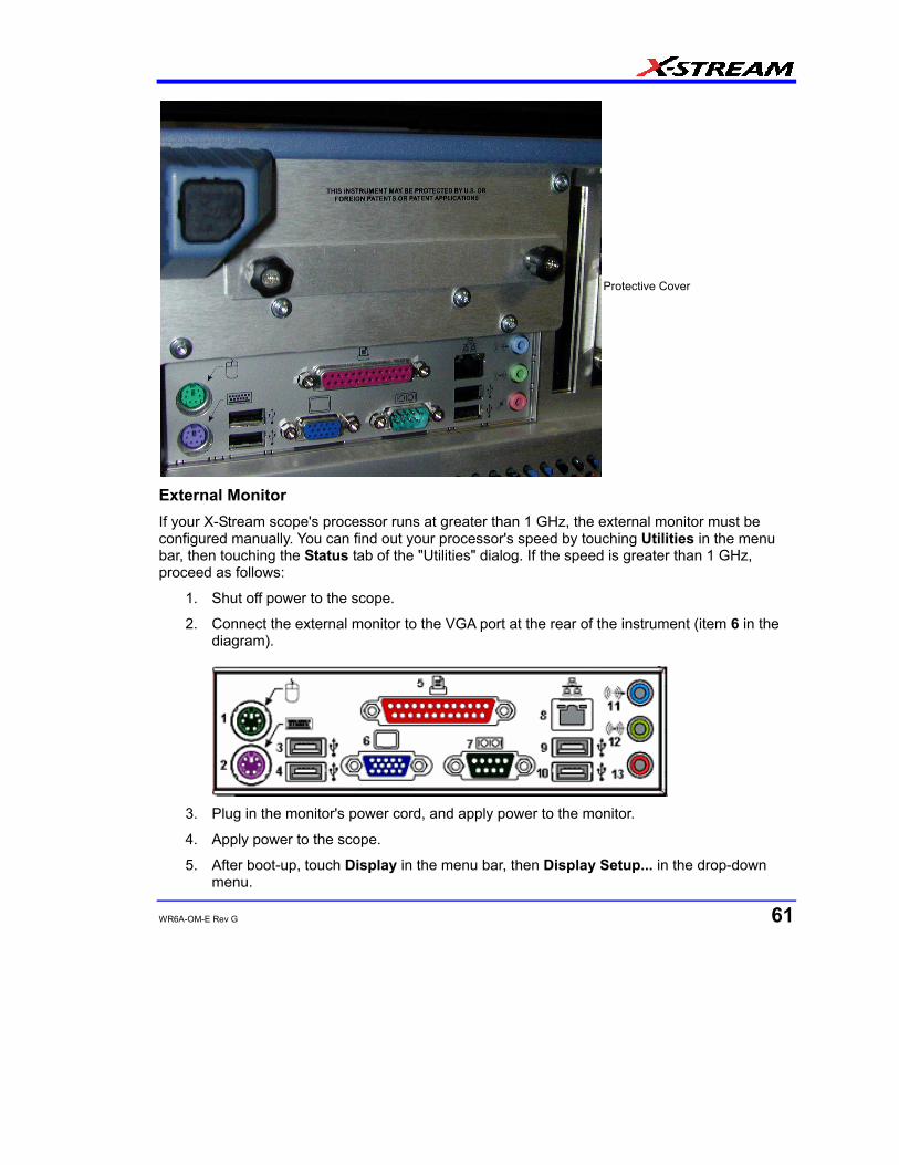
WR6A-OM-E Rev G 61
Protective Cover
External Monitor If your X-Stream scope's processor runs at greater than 1 GHz, the external monitor must be configured manually. You can find out your processor's speed by touching Utilities in the menu bar, then touching the Status tab of the "Utilities" dialog. If the speed is greater than 1 GHz, proceed as follows:
1. Shut off power to the scope.
2. Connect the external monitor to the VGA port at the rear of the instrument (item 6 in the diagram).
3. Plug in the monitor's power cord, and apply power to the monitor.
4. Apply power to the scope.
5. After boot-up, touch Display in the menu bar, then Display Setup... in the drop-down menu.
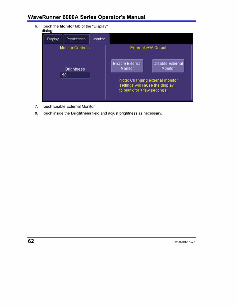
WaveRunner 6000A Series Operator's Manual
62 WR6A-OM-E Rev G
6. Touch the Monitor tab of the "Display" dialog:
7. Touch Enable External Monitor.
8. Touch inside the Brightness field and adjust brightness as necessary.
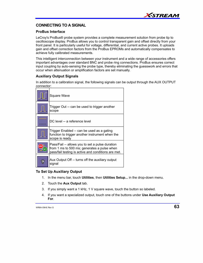
WR6A-OM-E Rev G 63
CONNECTING TO A SIGNAL ProBus Interface LeCroy's ProBus® probe system provides a complete measurement solution from probe tip to oscilloscope display. ProBus allows you to control transparent gain and offset directly from your front panel. It is particularly useful for voltage, differential, and current active probes. It uploads gain and offset correction factors from the ProBus EPROMs and automatically compensates to achieve fully calibrated measurements.
This intelligent interconnection between your instrument and a wide range of accessories offers important advantages over standard BNC and probe ring connections. ProBus ensures correct input coupling by auto-sensing the probe type, thereby eliminating the guesswork and errors that occur when attenuation or amplification factors are set manually.
Auxiliary Output Signals In addition to a calibration signal, the following signals can be output through the AUX OUTPUT connector:
Square Wave
Trigger Out -- can be used to trigger another scope
DC level -- a reference level
Trigger Enabled -- can be used as a gating function to trigger another instrument when the scope is ready
Pass/Fail -- allows you to set a pulse duration from 1 ms to 500 ms; generates a pulse when pass/fail testing is active and conditions are met.
Aux Output Off -- turns off the auxiliary output signal
To Set Up Auxiliary Output 1. In the menu bar, touch Utilities, then Utilities Setup... in the drop-down menu.
2. Touch the Aux Output tab.
3. If you simply want a 1 kHz, 1 V square wave, touch the button so labeled.
4. If you want a specialized output, touch one of the buttons under Use Auxiliary Output For.

WaveRunner 6000A Series Operator's Manual
64 WR6A-OM-E Rev G
5. Touch inside the Amplitude data entry field and enter a value, using the pop-up numeric keypad. If you want a TTL level signal, touch the TTL Level checkbox. The Amplitude field will accordingly become unavailable.
6. If you selected Square Wave, touch inside the Frequency data entry field and enter a value, using the pop-up keypad. You can set a value from 5.0 Hz to 5 MHz.
7. If you selected Pass/Fail, touch inside the Pulse Duration field and enter a value from 1 ms to 500 ms, using the pop-up numeric keypad.
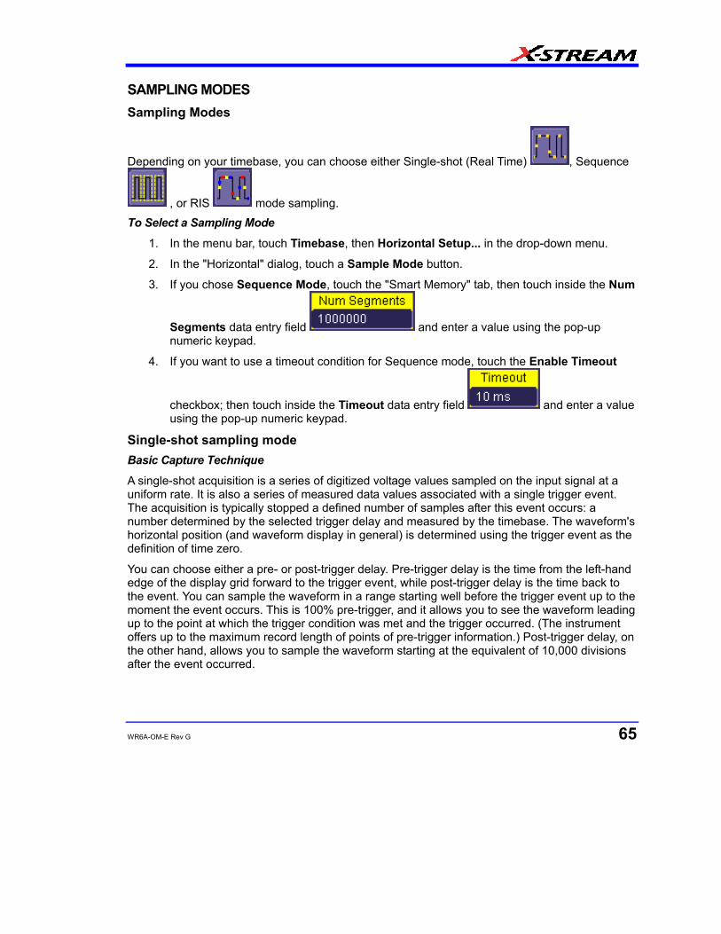
WR6A-OM-E Rev G 65
SAMPLING MODES Sampling Modes
Depending on your timebase, you can choose either Single-shot (Real Time) , Sequence
, or RIS mode sampling. To Select a Sampling Mode
1. In the menu bar, touch Timebase, then Horizontal Setup... in the drop-down menu.
2. In the "Horizontal" dialog, touch a Sample Mode button.
3. If you chose Sequence Mode, touch the "Smart Memory" tab, then touch inside the Num
Segments data entry field and enter a value using the pop-up numeric keypad.
4. If you want to use a timeout condition for Sequence mode, touch the Enable Timeout
checkbox; then touch inside the Timeout data entry field and enter a value using the pop-up numeric keypad.
Single-shot sampling mode Basic Capture Technique
A single-shot acquisition is a series of digitized voltage values sampled on the input signal at a uniform rate. It is also a series of measured data values associated with a single trigger event. The acquisition is typically stopped a defined number of samples after this event occurs: a number determined by the selected trigger delay and measured by the timebase. The waveform's horizontal position (and waveform display in general) is determined using the trigger event as the definition of time zero.
You can choose either a pre- or post-trigger delay. Pre-trigger delay is the time from the left-hand edge of the display grid forward to the trigger event, while post-trigger delay is the time back to the event. You can sample the waveform in a range starting well before the trigger event up to the moment the event occurs. This is 100% pre-trigger, and it allows you to see the waveform leading up to the point at which the trigger condition was met and the trigger occurred. (The instrument offers up to the maximum record length of points of pre-trigger information.) Post-trigger delay, on the other hand, allows you to sample the waveform starting at the equivalent of 10,000 divisions after the event occurred.
WaveRunner 6000A Series Operator's Manual
66 WR6A-OM-E Rev G
Because each instrument input channel has a dedicated ADC (Analog-to-Digital Converter), the voltage on each is sampled and measured at the same instant. This allows very reliable time measurements between the channels.
On fast timebase settings, the maximum single-shot sampling rate is used. But for slower timebases, the sampling rate is decreased and the number of data samples maintained.
The relationship between sample rate, memory, and time can be simply defined as:
and
Sequence SAMPLING Mode Working With Segments In sequence mode, the complete waveform consists of a number of fixed-size segments acquired in single-shot mode (see the instrument specifications for the limits). Select the number of segments to be captured, then select each segment individually and use it for processing with math and measure tools.
Sequence mode offers a number of unique capabilities. With it, you can limit dead time between trigger events for consecutive segments. The instrument can capture in fine detail complicated sequences of events over large time intervals, while ignoring the uninteresting periods between the events. You can also make time measurements between events on selected segments using the full precision of the acquisition timebase.
Each individual segment can be zoomed or used as input to math functions.
The instrument uses the sequence timebase setting to determine the capture duration of each segment: 10 x time/div. Along with this setting, the scope uses the desired number of segments, maximum segment length, and total available memory to determine the actual number of samples or segments, and time or points. However, the display of the complete waveform with all its segments may not entirely fill the screen.
You can also use Sequence mode in remote operation to take full advantage of the instrument's high data-transfer capability.
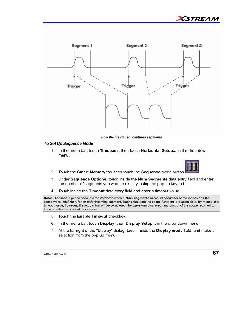
WR6A-OM-E Rev G 67
How the instrument captures segments
To Set Up Sequence Mode
1. In the menu bar, touch Timebase, then touch Horizontal Setup... in the drop-down menu.
2. Touch the Smart Memory tab, then touch the Sequence mode button .
3. Under Sequence Options, touch inside the Num Segments data entry field and enter the number of segments you want to display, using the pop-up keypad.
4. Touch inside the Timeout data entry field and enter a timeout value. Note: The timeout period accounts for instances when a Num Segments miscount occurs for some reason and the scope waits indefinitely for an unforthcoming segment. During that time, no scope functions are accessible. By means of a timeout value, however, the acquisition will be completed, the waveform displayed, and control of the scope returned to the user after the timeout has elapsed.
5. Touch the Enable Timeout checkbox.
6. In the menu bar, touch Display, then Display Setup... in the drop-down menu.
7. At the far right of the "Display" dialog, touch inside the Display mode field, and make a selection from the pop-up menu.
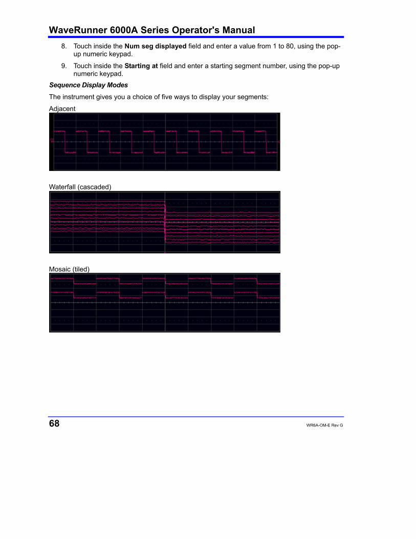
WaveRunner 6000A Series Operator's Manual
68 WR6A-OM-E Rev G
8. Touch inside the Num seg displayed field and enter a value from 1 to 80, using the pop-up numeric keypad.
9. Touch inside the Starting at field and enter a starting segment number, using the pop-up numeric keypad.
Sequence Display Modes
The instrument gives you a choice of five ways to display your segments:
Adjacent
Waterfall (cascaded)
Mosaic (tiled)

WR6A-OM-E Rev G 69
Overlay
Perspective
The number of segments you choose to display (80 maximum) can be less than the total number of segments in the waveform. For example, in the pop-up images above, the number of display segments is 10, but the total number of segments entered in the timebase dialog's Num Segments field is 100. To Display Individual Segments
1. Touch Math in the menu bar, then Math Setup... in the drop-down menu.
2. Touch a function tab (F1 to Fx The number of math traces available depends on the software options loaded on your scope. See specifications.).
3. Touch inside the Operator1 field and select Segment from the pop-up menu.
4. In the right-hand dialog, touch the Select tab.
5. Touch inside the Select data entry field and use the pop-up numeric keypad to select the segment you want to display.
Note: In Persistence mode, the segments are automatically overlaid one on top of the other in the display. In non-Persistence mode, they appear separately on the grid.
To View Time Stamps
1. In the menu bar, touch Timebase, then touch Acquisition Status... in the drop-down menu.
2. Touch the Time tab.
3. Touch one of the channel buttons under Select Waveform.
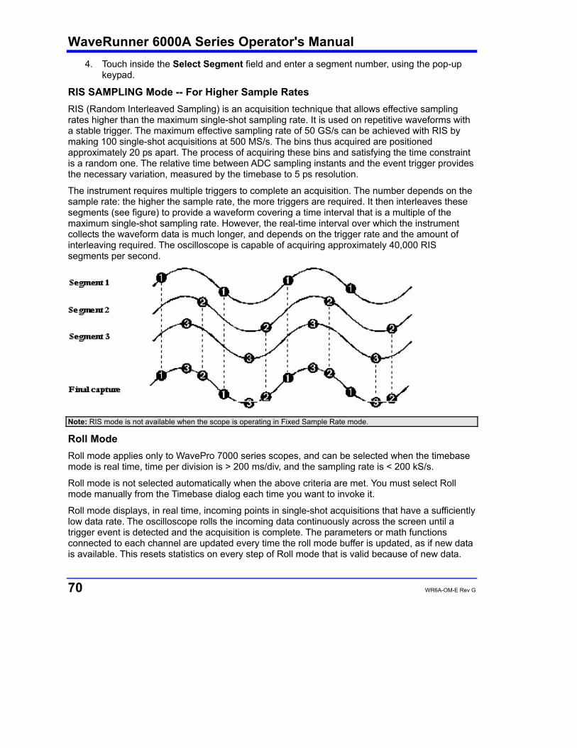
WaveRunner 6000A Series Operator's Manual
70 WR6A-OM-E Rev G
4. Touch inside the Select Segment field and enter a segment number, using the pop-up keypad.
RIS SAMPLING Mode -- For Higher Sample Rates RIS (Random Interleaved Sampling) is an acquisition technique that allows effective sampling rates higher than the maximum single-shot sampling rate. It is used on repetitive waveforms with a stable trigger. The maximum effective sampling rate of 50 GS/s can be achieved with RIS by making 100 single-shot acquisitions at 500 MS/s. The bins thus acquired are positioned approximately 20 ps apart. The process of acquiring these bins and satisfying the time constraint is a random one. The relative time between ADC sampling instants and the event trigger provides the necessary variation, measured by the timebase to 5 ps resolution.
The instrument requires multiple triggers to complete an acquisition. The number depends on the sample rate: the higher the sample rate, the more triggers are required. It then interleaves these segments (see figure) to provide a waveform covering a time interval that is a multiple of the maximum single-shot sampling rate. However, the real-time interval over which the instrument collects the waveform data is much longer, and depends on the trigger rate and the amount of interleaving required. The oscilloscope is capable of acquiring approximately 40,000 RIS segments per second.
Note: RIS mode is not available when the scope is operating in Fixed Sample Rate mode.
Roll Mode Roll mode applies only to WavePro 7000 series scopes, and can be selected when the timebase mode is real time, time per division is > 200 ms/div, and the sampling rate is < 200 kS/s.
Roll mode is not selected automatically when the above criteria are met. You must select Roll mode manually from the Timebase dialog each time you want to invoke it.
Roll mode displays, in real time, incoming points in single-shot acquisitions that have a sufficiently low data rate. The oscilloscope rolls the incoming data continuously across the screen until a trigger event is detected and the acquisition is complete. The parameters or math functions connected to each channel are updated every time the roll mode buffer is updated, as if new data is available. This resets statistics on every step of Roll mode that is valid because of new data.
WR6A-OM-E Rev G 71
Note: If the processing time is greater than the acquire time, the data in memory gets overwritten. In this case, the instrument issues the warning: Channel data is not continuous in ROLL mode!!! and rolling will start over again.
VERTICAL SETTINGS AND CHANNEL CONTROLS Adjusting Sensitivity and Position To Adjust Sensitivity
1. Press the appropriate channel push button, for example to turn on channel 1. Or touch Vertical in the menu bar, then Channel 1 in the drop-down menu.
2. Touch inside the Trace On checkbox to display the trace.
3. Turn the volts per division knob for the selected channel. Or you can touch inside the Volts/Div field and type in a value using the pop-up keypad, or use the up/down arrows.
4. The voltage that you set is displayed in the trace descriptor label and in the Volts/Div field.
To Adjust the Waveform's Position
Turn the vertical offset adjust knob directly above the channel button whose waveform you want to move vertically. Or you can touch inside the Offset field and type in a value on the pop-up keypad. To set the vertical offset to zero, touch the Zero Offset button directly below the Offset field.
Coupling The choices of coupling are as follows:
• DC 50 (all instruments)
• GROUND (all instruments)
• DC 1 M (WavePro & WaveRunner instruments)
• AC 1 M (WavePro & WaveRunner instruments) Overload Protection
The maximum input voltage is 4 V peak. Whenever the voltage exceeds this limit, the coupling mode automatically switches from DC 50 to GROUND. You will then have to manually reset the coupling to DC 50 , as described next.

WaveRunner 6000A Series Operator's Manual
72 WR6A-OM-E Rev G
To Set Coupling
1. In the menu bar, touch the Vertical button, then Channel X Setup... in the drop-down menu.
2. Touch inside the Coupling field and select a coupling mode from the pop-up menu.
Probe Attenuation To Set Probe Attenuation
LeCroy's ProBus® system automatically senses probes and sets their attenuation for you. If you want to set the attenuation manually,
1. In the menu bar, touch Vertical, then select a channel from the drop-down menu.
2. Touch inside the Probe Atten. data entry field . Touch a divide-by menu selection or touch Var (variable). If you choose Var, type in a value using the pop-up numeric keypad.
Bandwidth Limit Reducing the bandwidth also reduces the signal and system noise, and prevents high frequency aliasing. To Set Bandwidth Limiting
1. To set bandwidth limiting
2. In the menu bar, touch Vertical, then select a channel from the drop-down menu.
3. Touch inside the Bandwidth field and select a bandwidth limit value from the pop-up menu. The options are
• Full (all X-Stream scopes)
• 4 GHz (WaveMaster 8600A/8500A, DDA-5005A, SDA)
• 3 GHz (WaveMaster 8600A/8500A, DDA-5005A, SDA)
• 1 GHz (WaveMaster DSOs, DDA-5005A, SDA)
• 200 MHz (all X-Stream scopes)
• 20 MHz (all X-Stream scopes)
Linear and (SinX)/X Interpolation Linear interpolation, which inserts a straight line between sample point, is best used to reconstruct straight-edged signals such as square waves. (Sinx)/x interpolation, on the other hand, is suitable for reconstructing curved or irregular waveshapes, especially when the sample rate is 3 to 5 times the system bandwidth.
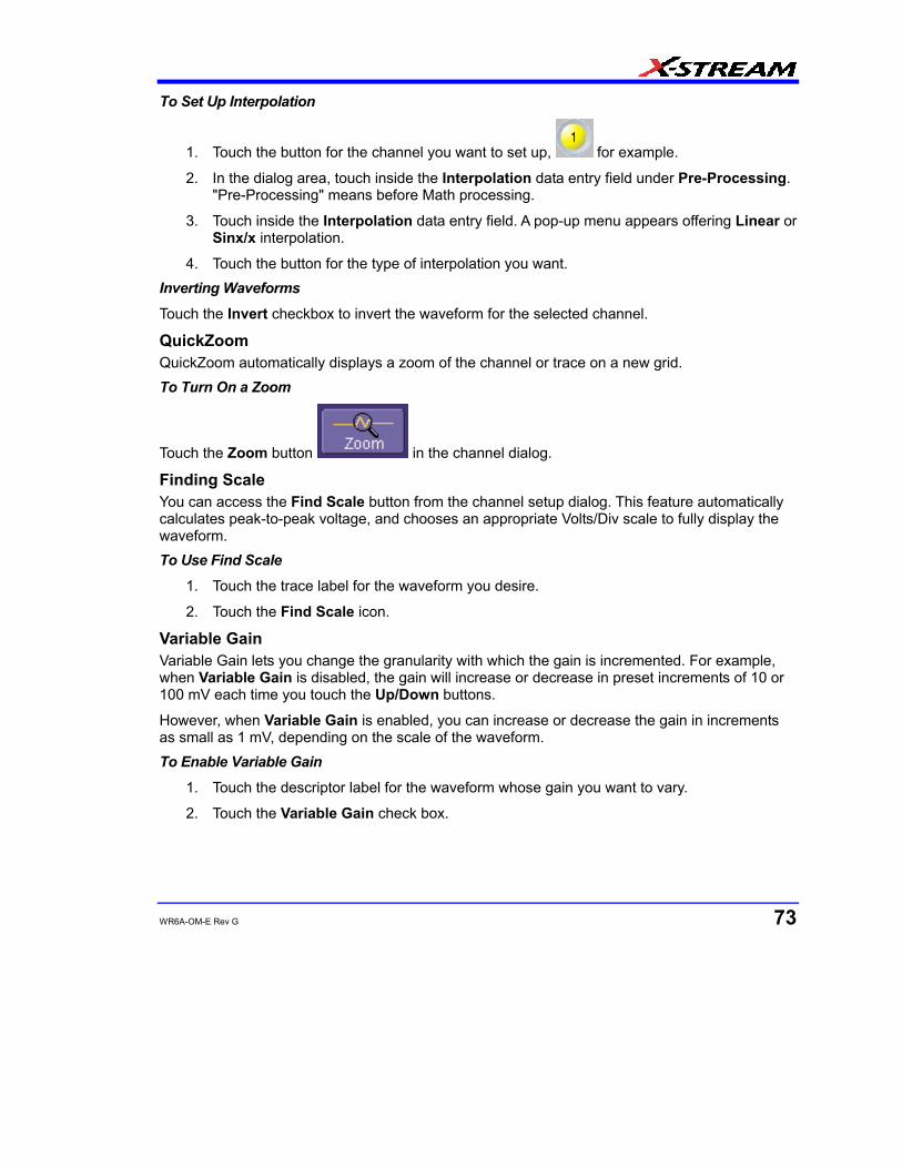
WR6A-OM-E Rev G 73
To Set Up Interpolation
1. Touch the button for the channel you want to set up, for example.
2. In the dialog area, touch inside the Interpolation data entry field under Pre-Processing. "Pre-Processing" means before Math processing.
3. Touch inside the Interpolation data entry field. A pop-up menu appears offering Linear or Sinx/x interpolation.
4. Touch the button for the type of interpolation you want. Inverting Waveforms
Touch the Invert checkbox to invert the waveform for the selected channel.
QuickZoom QuickZoom automatically displays a zoom of the channel or trace on a new grid. To Turn On a Zoom
Touch the Zoom button in the channel dialog.
Finding Scale You can access the Find Scale button from the channel setup dialog. This feature automatically calculates peak-to-peak voltage, and chooses an appropriate Volts/Div scale to fully display the waveform. To Use Find Scale
1. Touch the trace label for the waveform you desire.
2. Touch the Find Scale icon.
Variable Gain Variable Gain lets you change the granularity with which the gain is incremented. For example, when Variable Gain is disabled, the gain will increase or decrease in preset increments of 10 or 100 mV each time you touch the Up/Down buttons.
However, when Variable Gain is enabled, you can increase or decrease the gain in increments as small as 1 mV, depending on the scale of the waveform. To Enable Variable Gain
1. Touch the descriptor label for the waveform whose gain you want to vary.
2. Touch the Variable Gain check box.

WaveRunner 6000A Series Operator's Manual
74 WR6A-OM-E Rev G
Channel Deskew Unlike the Deskew math function, channel Deskew does no resampling, but instead adjusts the horizontal offset by the amount that you enter. The valid range is dependent on the current timebase +/- 9 divisions. To Set Up Channel Deskew
1. In the menu bar, touch Vertical; from the drop-down menu, select a channel to set up.
2. Touch inside the Deskew data entry field and enter a value using the pop-up numeric keypad.

WR6A-OM-E Rev G 75
TIMEBASE AND ACQUISITION SYSTEM Timebase Setup and Control Set up the timebase by using the front panel Horizontal controls, just as for analog scopes.
For additional timebase setups,
1. Touch Timebase in the menu bar, then Horizontal Setup... in the drop-down menu. The "Horizontal" dialog appears.
2. Touch inside the Time/Division data entry field and enter a value using the pop-up numeric keypad, or use the up/down arrows to adjust the value.
3. Touch inside the Delay data entry field and type in a value, using the pop-up keypad. Touch the Set To Zero button to set the delay to zero.
4. Touch the SMART Memory button or tab and adjust the memory as needed.
Dual Channel Acquisition Combining of Channels
Channels can be combined to increase sample rate, memory, or both in order to capture and view a signal in all its detail. When you combine channels, uncombined channels like EXT BNC remain available for triggering, even though they are not displayed. Note: While channels can be combined on any WaveRunner 6000 Series model to increase memory, sample rate can only be increased on 1 GHz and 2 GHz bandwidth models.
In 2-channel operation, channels 2 and 3 are active. In Auto operation, you can use channel 1 or 2, and channel 3 or 4. On the paired channels the maximum sampling rate is doubled and the record length is greatly increased:
Ch 1 & Ch 3 10 GS/s
Ch 1 & Ch 4 10 GS/s
Ch 2 & Ch 3 10 GS/s
Ch 2 & Ch 4 10 GS/s
As you can see, sampling can be maximized to 10 GS/s for any combination of two channels, except a combination of channels 1 and 2, or channels 3 and 4, which yield 5 GS/s. The basic rule is to choose either channel 1 or 2 for your first input, and either channel 3 or 4 for the second input.
Refer to Acquisition Modes in the specifications for maximum sample rates. To Combine Channels
1. In the menu bar, touch Timebase; the "Horizontal" setup dialog opens.
2. Under Active Channels, touch 4, 2 or Auto. The maximum sample rate is shown alongside each button.

WaveRunner 6000A Series Operator's Manual
76 WR6A-OM-E Rev G
Autosetup When channels are turned on, Autosetup operates only on those turned-on channels. If no channels are turned on, all channels are affected. When more than one channel is turned on, the first channel in numerical order with a signal applied to it is automatically set up for edge triggering.
You can perform an autosetup of all these functions together by simply pressing on the
front panel, or by touching Autosetup in any drop-down menu.

WR6A-OM-E Rev G 77
TRIGGERING Trigger Setup Considerations Trigger Modes
Auto mode causes the scope to sweep even without a trigger. An internal timer triggers the sweep so that the display remains, even when the signal does not cause a trigger.
In Normal mode, the scope sweeps only if the input signal reaches the set trigger point. Otherwise it continues to display the last acquired waveform.
In Single mode, only one sweep occurs each time you press the button.
Stop mode inhibits all sweeps until you select one of the other three modes. Trigger Types
The triggers available to you are defined as follows:
A simple trigger, Edge trigger is activated by basic waveform features or conditions such as positive or negative slope, and holdoff.
One of LeCroy's SMART Triggers®, Width trigger allows you to define a positive- or negative-going pulse width bounded by a voltage level, above or below which a trigger will occur. Or you can specify a pulse width and voltage range, within or outside of which a trigger will occur.
Another of the SMART Triggers, Glitch trigger is a simpler form of Width trigger. Use Glitch trigger when you want to define a fixed pulse-width time or time range only. Glitch trigger makes no provision for voltage levels or ranges.
While Glitch trigger performs over the width of a pulse, Interval trigger performs over the width of an interval the signal duration (the period) separating two consecutive edges of the same polarity: positive to positive or negative to negative. Use interval trigger to capture intervals that fall short of, or exceed, a given time limit. In addition, you can define a width range to capture any interval that is itself inside or outside the specified range an Exclusion trigger by interval.
The Qualify trigger is an edge-qualified SMART Trigger that allows you to use one signal's positive or negative transition to qualify a second signal, which is the trigger source. For Qualify trigger, you specify the time or number of events after the transition when you want the trigger to occur.
The State trigger is a level-qualified SMART Trigger which requires that the qualifying signal remain above or below a specified voltage level for a trigger to occur. For Sate trigger, you specify the time or number of events after the signal has gone above or below the voltage level when you want the trigger to occur.

WaveRunner 6000A Series Operator's Manual
78 WR6A-OM-E Rev G
Used primarily in single-shot applications, and usually with a pre-trigger delay, Dropout trigger can detect lost signals. The trigger is generated at the end of the timeout period following the last trigger source transition. You can select a timeout period from 2 ns to 20 s.
Logic trigger enables triggering on a logical combination (pattern) of five inputs: CH1, CH2, CH3, CH4, EXT. You have a choice of four Boolean operators (AND, NAND, OR, NOR), and you can stipulate the high or low voltage logic level for each input independently.
Determining Trigger Level, Slope, Source, and Coupling Level defines the source voltage at which the trigger circuit will generate an event: a change in the input signal that satisfies the trigger conditions. The selected trigger level is associated with the chosen trigger source.
Trigger level is specified in volts and normally remains unchanged when you change the vertical gain or offset. The amplitude and range of the trigger level are limited as follows:
• ±5 screen divisions with a channel as the trigger source
• ±400 mV with EXT as the trigger source
• ±4 V with EXT/10 as the trigger source
• ±40 mV with EXT*10 as the trigger source
• None with LINE as the trigger source (zero crossing is used).
Coupling refers to the type of signal coupling at the input of the trigger circuit. Because of the instrument's very high bandwidth, there is only one choice of trigger coupling: DC 50 ohms. However, as a visual check of where ground is, you may switch the channel to ground coupling at any time while testing.
With DC coupling, all of the signal's frequency components are coupled to the trigger circuit for high-frequency bursts.
Slope determines the direction of the trigger voltage transition used for generating a particular trigger event. You can choose a positive or negative slope. Like coupling, the selected slope is associated with the chosen trigger source.
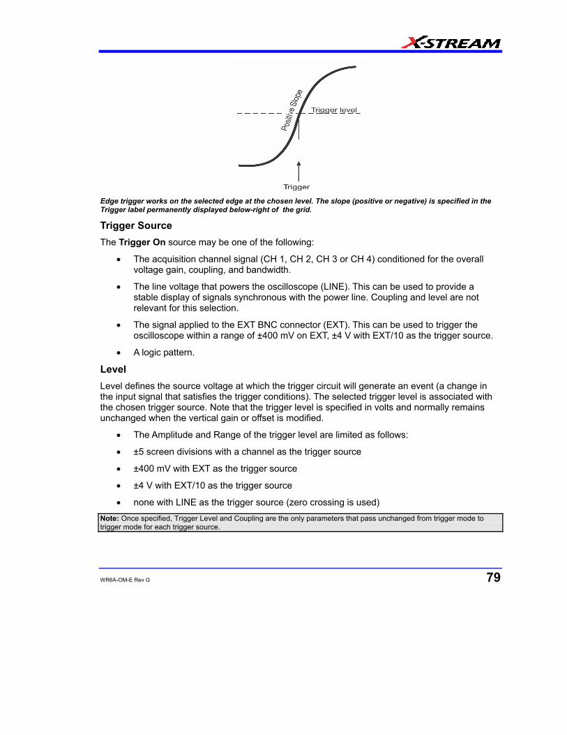
WR6A-OM-E Rev G 79
Edge trigger works on the selected edge at the chosen level. The slope (positive or negative) is specified in the Trigger label permanently displayed below-right of the grid. Trigger Source The Trigger On source may be one of the following:
• The acquisition channel signal (CH 1, CH 2, CH 3 or CH 4) conditioned for the overall voltage gain, coupling, and bandwidth.
• The line voltage that powers the oscilloscope (LINE). This can be used to provide a stable display of signals synchronous with the power line. Coupling and level are not relevant for this selection.
• The signal applied to the EXT BNC connector (EXT). This can be used to trigger the oscilloscope within a range of ±400 mV on EXT, ±4 V with EXT/10 as the trigger source.
• A logic pattern.
Level Level defines the source voltage at which the trigger circuit will generate an event (a change in the input signal that satisfies the trigger conditions). The selected trigger level is associated with the chosen trigger source. Note that the trigger level is specified in volts and normally remains unchanged when the vertical gain or offset is modified.
• The Amplitude and Range of the trigger level are limited as follows:
• ±5 screen divisions with a channel as the trigger source
• ±400 mV with EXT as the trigger source
• ±4 V with EXT/10 as the trigger source
• none with LINE as the trigger source (zero crossing is used) Note: Once specified, Trigger Level and Coupling are the only parameters that pass unchanged from trigger mode to trigger mode for each trigger source.

WaveRunner 6000A Series Operator's Manual
80 WR6A-OM-E Rev G
Holdoff by Time or Events Holdoff is an additional condition of Edge trigger. It can be expressed either as a period of time or an event count. Holdoff disables the trigger circuit for a given period of time or number of events after the last trigger occurred. Events are the number of occasions on which the trigger condition is met. The trigger will again occur when the holdoff has elapsed and the trigger's other conditions are met.
Use holdoff to obtain a stable trigger for repetitive, composite waveforms. For example, if the number or duration of sub-signals is known you can disable them by choosing an appropriate holdoff value. Qualified triggers operate using conditions similar to holdoff. Hold Off by Time
Sometimes you can achieve a stable display of complex, repetitive waveforms by placing a condition on the time between each successive trigger event. This time would otherwise be limited only by the input signal, the coupling, and the instrument's bandwidth. Select a positive or negative slope, and a minimum time between triggers. The trigger is generated when the condition is met after the selected holdoff time, counted from the last trigger. Any time between 2 ns and 20 s can be selected. The delay is initialized and started on each trigger.
Edge Trigger with Holdoff by Time. The bold edges on the trigger source indicate that a positive slope has been selected. The broken upward-pointing arrows indicate potential triggers, which would occur if other conditions are met. The bold arrows indicate where the triggers actually occur when the holdoff time has been exceeded. Hold Off by Events
Select a positive or negative slope and a number of events. An event is the number of times the trigger condition is met after the last trigger. A trigger is generated when the condition is met after this number, counted from the last trigger. The count is restarted on each trigger. For example, if the event number is two, the trigger will occur on the third event. From one to 1,000,000,000 events can be selected.

WR6A-OM-E Rev G 81
Edge Trigger with Holdoff by Events (in this example, two events). The bold edges on the trigger source indicate that a positive slope has been selected. The broken, upward-pointing arrows indicate potential triggers, while the bold ones show where triggers actually occur after the holdoff expires. Simple Triggers Edge Trigger on Simple Signals
The instrument uses many waveform capture techniques that trigger on features and conditions that you define. These triggers fall into two major categories:
Edge activated by basic waveform features or conditions such as a positive or negative slope, and hold-off
SMART Trigger® sophisticated triggers that enable you to use basic or complex conditions for triggering.
Use Edge Triggers for simple signals, and the SMART Triggers for signals with rare features, like glitches. Control Edge Triggering
Horizontal: Turn the Delay knob in the HORIZONTAL control group to adjust the trigger's horizontal position. Or, touch inside the Delay field in the timebase setup dialog and enter a value, using the pop-up keypad.
The trigger location is shown by a marker below the grid .
Post-trigger delay is indicated by a left-pointing arrow below-left of the grid . The time
value is given in the title line of the TimeBase label below-right of the grid.
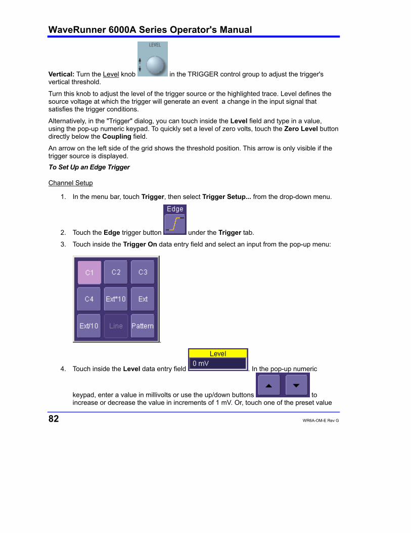
WaveRunner 6000A Series Operator's Manual
82 WR6A-OM-E Rev G
Vertical: Turn the Level knob in the TRIGGER control group to adjust the trigger's vertical threshold.
Turn this knob to adjust the level of the trigger source or the highlighted trace. Level defines the source voltage at which the trigger will generate an event a change in the input signal that satisfies the trigger conditions.
Alternatively, in the "Trigger" dialog, you can touch inside the Level field and type in a value, using the pop-up numeric keypad. To quickly set a level of zero volts, touch the Zero Level button directly below the Coupling field.
An arrow on the left side of the grid shows the threshold position. This arrow is only visible if the trigger source is displayed. To Set Up an Edge Trigger
Channel Setup
1. In the menu bar, touch Trigger, then select Trigger Setup... from the drop-down menu.
2. Touch the Edge trigger button under the Trigger tab.
3. Touch inside the Trigger On data entry field and select an input from the pop-up menu:
.
4. Touch inside the Level data entry field . In the pop-up numeric
keypad, enter a value in millivolts or use the up/down buttons to increase or decrease the value in increments of 1 mV. Or, touch one of the preset value

WR6A-OM-E Rev G 83
buttons:
.
Max. 1.000 V
Default 0 mV
Min. 1.000 V
5. Select the holdoff by touching the Time or Events buttons , . Using the pop-up numeric keypad, enter a value and specify the unit of time, or use the up/down
buttons to increase or decrease the time value in increments of 200 ps. Or, touch one of the preset value buttons:
.
6. The preset Time values are as follows:
Max. 20.0 s
Default 50.0 ns
Min. 2 ns

WaveRunner 6000A Series Operator's Manual
84 WR6A-OM-E Rev G
The preset Events values are as follows:
Max. 1,000,000,000 events
Default 1 event
Min. 1 event
7. Choose Positive or Negative slope
.
SMART Triggers Width Trigger
How Width Trigger Works
Width trigger allows you to define a positive- or negative-going pulse width bounded by a voltage level, above or below which a trigger will occur. You can specify a pulse width and voltage range, within or outside of which a trigger will occur.
To Set Up Width Trigger
1. In the menu bar, touch Trigger, then Trigger Setup... in the drop-down menu.
2. Touch the Width trigger button
3. Touch inside the Trigger On data entry field and select a source on which to trigger.

WR6A-OM-E Rev G 85
4. Touch inside the Level data entry field and enter a value using the pop-up numeric keypad.
5. Select positive or negative slope.
6. Touch the LessThan button and enter a pulse-width value in the Upper Limit data entry field. Or touch the GreaterThan button and enter a pulse-width value in the Lower Limit
data entry field. Or touch the InRange button. Touch the Delta button to set up a nominal range, plus or minus a delta value in seconds. Touch inside the Nominal Width and Delta data entry fields and enter values using the pop-up numeric keypads.
Alternatively, touch the Limits button to set up a precise pulse-width range. Touch inside the Lower Limit and Upper Limit data entry fields and enter values using the pop-up keypads. Or touch the OutOfRange button and perform the same range setups as for InRange triggering.
Glitch Trigger
How Glitch Trigger Works
Glitch trigger can be used to catch glitches. You can specify a pulse width or a pulse width range.
Pulse smaller than selected pulse width: Set a maximum pulse width. This glitch trigger is generated on the selected edge (positive or negative) when the pulse width is less than or equal to the set width.
The timing for the width is initialized and restarted on the opposite slope to that selected. You can set widths from 600 ps to 20 s. Note: If the glitch's width is narrower than the signal's width, set the trigger to a narrower width than that of the signal. The signal's width, as determined by the instrument trigger comparator, depends on the DC trigger level. If that level were to be set at the middle of a sine wave, for example, the width could then be considered as the half period. But if the level were higher, the signal's width would be considered to be less than the half period.
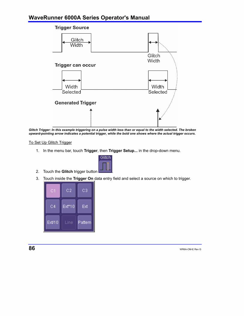
WaveRunner 6000A Series Operator's Manual
86 WR6A-OM-E Rev G
Glitch Trigger: In this example triggering on a pulse width less than or equal to the width selected. The broken upward-pointing arrow indicates a potential trigger, while the bold one shows where the actual trigger occurs.
To Set Up Glitch Trigger
1. In the menu bar, touch Trigger, then Trigger Setup... in the drop-down menu.
2. Touch the Glitch trigger button .
3. Touch inside the Trigger On data entry field and select a source on which to trigger.
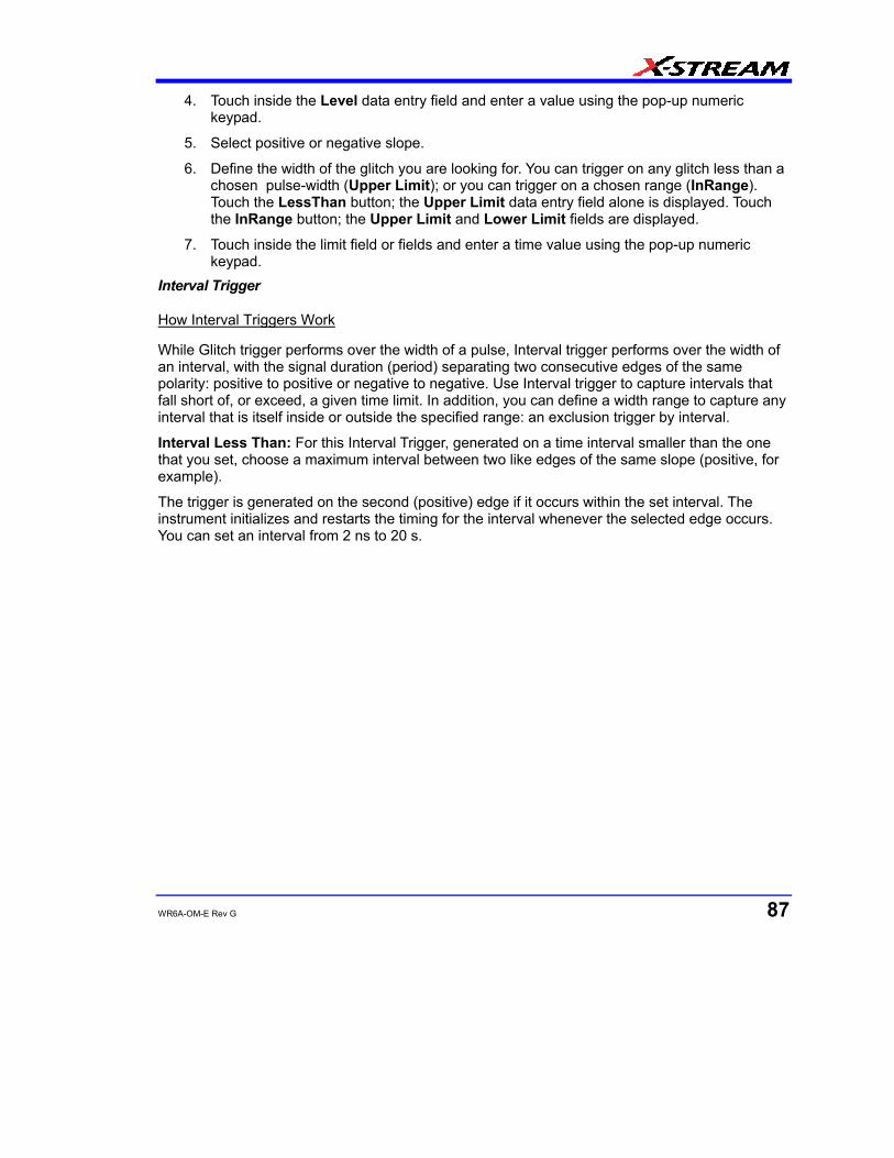
WR6A-OM-E Rev G 87
4. Touch inside the Level data entry field and enter a value using the pop-up numeric keypad.
5. Select positive or negative slope.
6. Define the width of the glitch you are looking for. You can trigger on any glitch less than a chosen pulse-width (Upper Limit); or you can trigger on a chosen range (InRange). Touch the LessThan button; the Upper Limit data entry field alone is displayed. Touch the InRange button; the Upper Limit and Lower Limit fields are displayed.
7. Touch inside the limit field or fields and enter a time value using the pop-up numeric keypad.
Interval Trigger
How Interval Triggers Work
While Glitch trigger performs over the width of a pulse, Interval trigger performs over the width of an interval, with the signal duration (period) separating two consecutive edges of the same polarity: positive to positive or negative to negative. Use Interval trigger to capture intervals that fall short of, or exceed, a given time limit. In addition, you can define a width range to capture any interval that is itself inside or outside the specified range: an exclusion trigger by interval.
Interval Less Than: For this Interval Trigger, generated on a time interval smaller than the one that you set, choose a maximum interval between two like edges of the same slope (positive, for example).
The trigger is generated on the second (positive) edge if it occurs within the set interval. The instrument initializes and restarts the timing for the interval whenever the selected edge occurs. You can set an interval from 2 ns to 20 s.
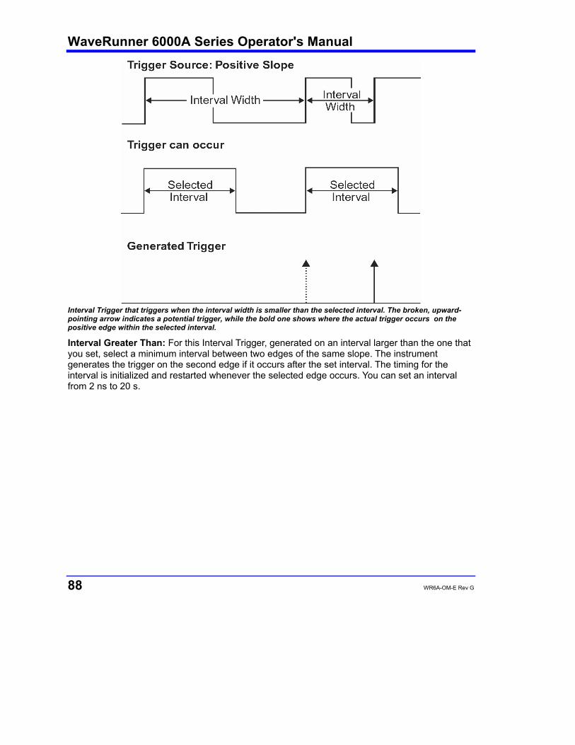
WaveRunner 6000A Series Operator's Manual
88 WR6A-OM-E Rev G
Interval Trigger that triggers when the interval width is smaller than the selected interval. The broken, upward-pointing arrow indicates a potential trigger, while the bold one shows where the actual trigger occurs on the positive edge within the selected interval. Interval Greater Than: For this Interval Trigger, generated on an interval larger than the one that you set, select a minimum interval between two edges of the same slope. The instrument generates the trigger on the second edge if it occurs after the set interval. The timing for the interval is initialized and restarted whenever the selected edge occurs. You can set an interval from 2 ns to 20 s.
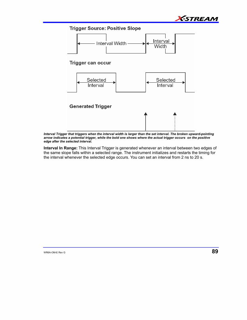
WR6A-OM-E Rev G 89
Interval Trigger that triggers when the interval width is larger than the set interval. The broken upward-pointing arrow indicates a potential trigger, while the bold one shows where the actual trigger occurs on the positive edge after the selected interval. Interval In Range: This Interval Trigger is generated whenever an interval between two edges of the same slope falls within a selected range. The instrument initializes and restarts the timing for the interval whenever the selected edge occurs. You can set an interval from 2 ns to 20 s.
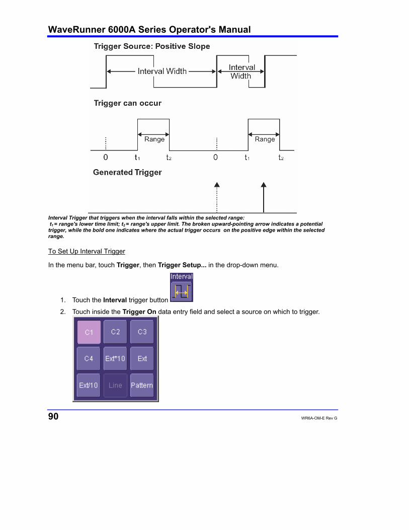
WaveRunner 6000A Series Operator's Manual
90 WR6A-OM-E Rev G
Interval Trigger that triggers when the interval falls within the selected range: t1 = range's lower time limit; t2 = range's upper limit. The broken upward-pointing arrow indicates a potential trigger, while the bold one indicates where the actual trigger occurs on the positive edge within the selected range.
To Set Up Interval Trigger
In the menu bar, touch Trigger, then Trigger Setup... in the drop-down menu.
1. Touch the Interval trigger button
2. Touch inside the Trigger On data entry field and select a source on which to trigger.
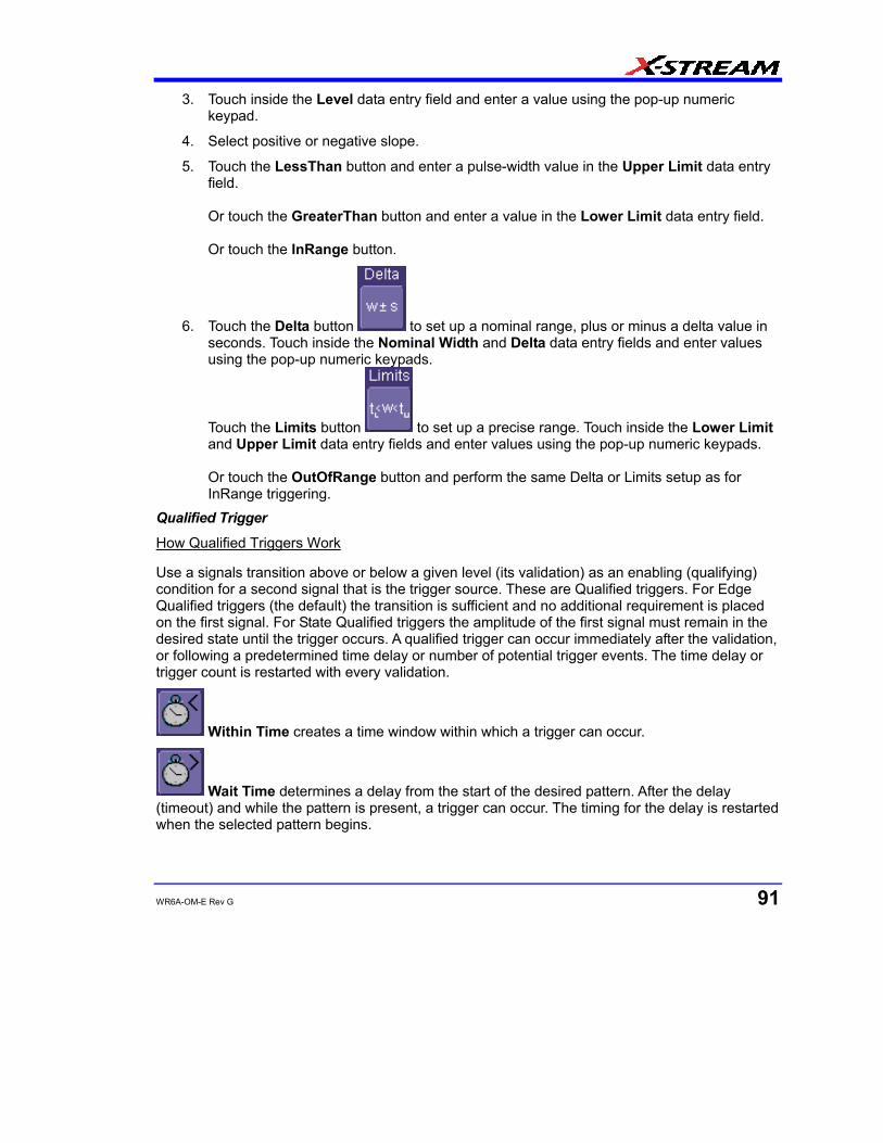
WR6A-OM-E Rev G 91
3. Touch inside the Level data entry field and enter a value using the pop-up numeric keypad.
4. Select positive or negative slope.
5. Touch the LessThan button and enter a pulse-width value in the Upper Limit data entry field. Or touch the GreaterThan button and enter a value in the Lower Limit data entry field. Or touch the InRange button.
6. Touch the Delta button to set up a nominal range, plus or minus a delta value in seconds. Touch inside the Nominal Width and Delta data entry fields and enter values using the pop-up numeric keypads.
Touch the Limits button to set up a precise range. Touch inside the Lower Limit and Upper Limit data entry fields and enter values using the pop-up numeric keypads. Or touch the OutOfRange button and perform the same Delta or Limits setup as for InRange triggering.
Qualified Trigger
How Qualified Triggers Work
Use a signals transition above or below a given level (its validation) as an enabling (qualifying) condition for a second signal that is the trigger source. These are Qualified triggers. For Edge Qualified triggers (the default) the transition is sufficient and no additional requirement is placed on the first signal. For State Qualified triggers the amplitude of the first signal must remain in the desired state until the trigger occurs. A qualified trigger can occur immediately after the validation, or following a predetermined time delay or number of potential trigger events. The time delay or trigger count is restarted with every validation.
Within Time creates a time window within which a trigger can occur.
Wait Time determines a delay from the start of the desired pattern. After the delay (timeout) and while the pattern is present, a trigger can occur. The timing for the delay is restarted when the selected pattern begins.
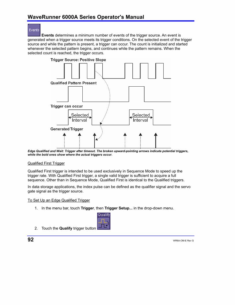
WaveRunner 6000A Series Operator's Manual
92 WR6A-OM-E Rev G
Events determines a minimum number of events of the trigger source. An event is generated when a trigger source meets its trigger conditions. On the selected event of the trigger source and while the pattern is present, a trigger can occur. The count is initialized and started whenever the selected pattern begins, and continues while the pattern remains. When the selected count is reached, the trigger occurs.
Edge Qualified and Wait: Trigger after timeout. The broken upward-pointing arrows indicate potential triggers, while the bold ones show where the actual triggers occur.
Qualified First Trigger
Qualified First trigger is intended to be used exclusively in Sequence Mode to speed up the trigger rate. With Qualified First trigger, a single valid trigger is sufficient to acquire a full sequence. Other than in Sequence Mode, Qualified First is identical to the Qualified triggers.
In data storage applications, the index pulse can be defined as the qualifier signal and the servo gate signal as the trigger source.
To Set Up an Edge Qualified Trigger
1. In the menu bar, touch Trigger, then Trigger Setup... in the drop-down menu.
2. Touch the Qualify trigger button
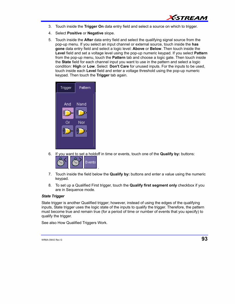
WR6A-OM-E Rev G 93
3. Touch inside the Trigger On data entry field and select a source on which to trigger.
4. Select Positive or Negative slope.
5. Touch inside the After data entry field and select the qualifying signal source from the pop-up menu. If you select an input channel or external source, touch inside the has gone data entry field and select a logic level: Above or Below. Then touch inside the Level field and set a voltage level using the pop-up numeric keypad. If you select Pattern from the pop-up menu, touch the Pattern tab and choose a logic gate. Then touch inside the State field for each channel input you want to use in the pattern and select a logic condition: High or Low. Select Don't Care for unused inputs. For the inputs to be used, touch inside each Level field and enter a voltage threshold using the pop-up numeric keypad. Then touch the Trigger tab again.
6. If you want to set a holdoff in time or events, touch one of the Qualify by: buttons:
, , .
7. Touch inside the field below the Qualify by: buttons and enter a value using the numeric keypad.
8. To set up a Qualified First trigger, touch the Qualify first segment only checkbox if you are in Sequence mode.
State Trigger
State trigger is another Qualified trigger; however, instead of using the edges of the qualifying inputs, State trigger uses the logic state of the inputs to qualify the trigger. Therefore, the pattern must become true and remain true (for a period of time or number of events that you specify) to qualify the trigger.
See also How Qualified Triggers Work.
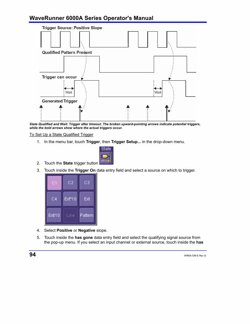
WaveRunner 6000A Series Operator's Manual
94 WR6A-OM-E Rev G
State Qualified and Wait: Trigger after timeout. The broken upward-pointing arrows indicate potential triggers, while the bold arrows show where the actual triggers occur. To Set Up a State Qualified Trigger
1. In the menu bar, touch Trigger, then Trigger Setup... in the drop-down menu.
2. Touch the State trigger button
3. Touch inside the Trigger On data entry field and select a source on which to trigger.
4. Select Positive or Negative slope.
5. Touch inside the has gone data entry field and select the qualifying signal source from the pop-up menu. If you select an input channel or external source, touch inside the has
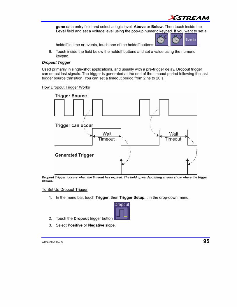
WR6A-OM-E Rev G 95
gone data entry field and select a logic level: Above or Below. Then touch inside the Level field and set a voltage level using the pop-up numeric keypad. If you want to set a
holdoff in time or events, touch one of the holdoff buttons: , , .
6. Touch inside the field below the holdoff buttons and set a value using the numeric keypad.
Dropout Trigger
Used primarily in single-shot applications, and usually with a pre-trigger delay, Dropout trigger can detect lost signals. The trigger is generated at the end of the timeout period following the last trigger source transition. You can set a timeout period from 2 ns to 20 s.
How Dropout Trigger Works
Dropout Trigger: occurs when the timeout has expired. The bold upward-pointing arrows show where the trigger occurs.
To Set Up Dropout Trigger
1. In the menu bar, touch Trigger, then Trigger Setup... in the drop-down menu.
2. Touch the Dropout trigger button .
3. Select Positive or Negative slope.
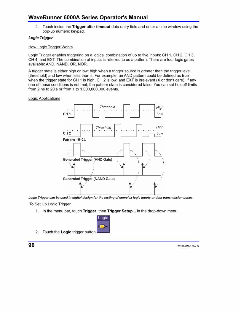
WaveRunner 6000A Series Operator's Manual
96 WR6A-OM-E Rev G
4. Touch inside the Trigger after timeout data entry field and enter a time window using the pop-up numeric keypad.
Logic Trigger
How Logic Trigger Works
Logic Trigger enables triggering on a logical combination of up to five inputs: CH 1, CH 2, CH 3, CH 4, and EXT. The combination of inputs is referred to as a pattern. There are four logic gates available: AND, NAND, OR, NOR.
A trigger state is either high or low: high when a trigger source is greater than the trigger level (threshold) and low when less than it. For example, an AND pattern could be defined as true when the trigger state for CH 1 is high, CH 2 is low, and EXT is irrelevant (X or don't care). If any one of these conditions is not met, the pattern state is considered false. You can set holdoff limits from 2 ns to 20 s or from 1 to 1,000,000,000 events.
Logic Applications
Logic Trigger can be used in digital design for the testing of complex logic inputs or data transmission buses. To Set Up Logic Trigger
1. In the menu bar, touch Trigger, then Trigger Setup... in the drop-down menu.
2. Touch the Logic trigger button .

WR6A-OM-E Rev G 97
3. Touch the Pattern tab.
4. For each input you want to include in the logic pattern, touch inside the State data entry field and select a logic state: Low or High. Select Don't Care for all other inputs.
5. Touch inside the Level data entry field for each input included in the pattern and enter a voltage level threshold using the pop-up numeric keypad.
6. Touch the Trigger tab.
7. If you want to hold off the trigger (either in time or events) when the pattern becomes
true, touch one of the holdoff buttons , .
8. Touch inside the holdoff data entry field and enter a value using the pop-up numeric keypad.

WaveRunner 6000A Series Operator's Manual
98 WR6A-OM-E Rev G
DISPLAY FORMATS Display Setup
1. In the menu bar, touch Display; then touch Display Setup in the drop-down menu.
2. Touch one of the Grid combination buttons. Autogrid automatically adds or deletes grids as you select more or fewer waveforms to display.
3. Touch inside the grid Intensity data entry field and enter a value from 0 to 100 using the pop-up keypad.
4. Touch the Grid on top checkbox if you want to superimpose the grid over the waveform. Depending on the grid intensity, some of your waveform may be hidden from view when the grid is placed on top. To undo, simply uncheck Grid on top.
5. Touch the Axis labels checkbox to permanently display the values of the top and bottom grid lines (calculated from volts/div) and the extreme left and right grid lines (calculated from the timebase).
6. Choose a line style for your trace: solid Line or Points . Sequence Mode Display
1. To a set up Sequence Mode display, you must first have selected Sequence trigger mode in the Timebase "Horizontal" dialog. You must also have entered a Num Segments value.
2. In the menu bar, touch Display; then touch Display Setup in the drop-down menu.
3. Touch inside the Display Mode field and select a display mode from the pop-up menu.
4. Touch inside the Num seg displayed field and enter a value, using the pop-up keypad. The maximum number of segments that can be displayed is 80.
WR6A-OM-E Rev G 99
5. Touch inside the Starting at field and enter a value. Note: The maximum value that you can enter for Starting at depends on the Num Segments value you entered in the "Timebase" dialog. It also depends on the Num seg displayed value you entered here in the "Display" dialog. For example, if you had entered a value of 500 in Num Segments, and a value of 10 in Num seg displayed, the maximum value you can enter as a starting segment is 491so that 10 segments can be seen.
Persistence Setup The analog Persistence feature helps you display your waveform and reveal its idiosyncrasies or anomalies for a repetitive signal. Use Persistence to accumulate on-screen points from many acquisitions to see your signal change over time. The instrument persistence modes show the most frequent signal path "three-dimensionally" in intensities of the same color, or graded in a spectrum of colors.
You can show persistence for up to eight inputs for any channel, math function, or memory location (M1 to M4). Saturation Level
The Persistence display is generated by repeated sampling of the amplitudes of events over time, and the accumulation of the sampled data into "3-dimensional" display maps. These maps create an analog-style display. User-definable persistence duration can be used to view how the maps evolve proportionally over time. Statistical integrity is preserved because the duration (decay) is proportional to the persistence population for each amplitude or time combination in the data. In addition, the instrument gives you post-acquisition saturation control for a more detailed display.
When you select mode from the Persistence dialog (with All Locked selected), each channel is assigned a single color. As a persistence data map develops, different intensities of that color are assigned to the range between a minimum and a maximum population. The maximum population automatically gets the highest intensity, the minimum population gets the lowest intensity, and intermediate populations get intensities in between these extremes.
The information in the lower populations (for example, down at the noise level) could be of greater interest to you than the rest. The Analog persistence view highlights the distribution of data so that you can examine it in detail.
You can select a saturation level as a percentage of the maximum population. All populations above the saturation population are then assigned the highest color intensity: that is, they are saturated. At the same time, all populations below the saturation level are assigned the remaining intensities. Data populations are dynamically updated as data from new acquisitions is accumulated.
Color mode persistence, selected by touching , works on the same principle as the Analog persistence feature, but instead uses the entire color spectrum to map signal intensity:

WaveRunner 6000A Series Operator's Manual
100 WR6A-OM-E Rev G
violet for minimum population, red for maximum population. A saturation level of 100% spreads the intensity variation across the entire distribution; at lower saturation levels the intensity will saturate (become the brightest color) at the percentage value specified. Lowering this percentage causes the pixels to be saturated at a lower population, and makes visible those rarely hit pixels not seen at higher percentages. 3-Dimensional Persistence
By selecting 3d , you can create a topographical view of your waveform from a selection of shadings, textures, and hues. The advantage of the topographical view is that areas of highest and lowest intensity are shown as peaks and valleys, in addition to color or brightness. The shape of the peaks (pointed or flat) can reveal further information about the frequency of occurrences in your waveform.
The instrument also gives you the ability to turn the X and Y axes of the waveform through 180° of rotation from -90° to +90°.
Here is an example of a 3-dimensional view of a square wave using the solid view of color-graded persistence. Saturation is set at 50%, with red areas indicating highest intensity. The X-axis has been rotated 60%; the Y-axis has been rotated 15%.
Here is a monochrome (analog) view of the same waveform. The lightest areas indicate highest intensity, corresponding to the red areas in the solid view.

WR6A-OM-E Rev G 101
Here is a shaded (projected light) view of the same waveform. This view emphasizes the shape of the pulses.
Here is a wire frame view of the same waveform in which lines of equal intensity are used to construct the persistence map.
Show Last Trace For most applications, you may not want to show the last trace because it will be superimposed on top of your persistence display. In those cases turn off Show Last Trace by touching the checkbox. However, if you are doing mask testing and want to see where the last trace is falling, turn Show Last Trace on.
Persistence Time You can control the duration of persistence by setting a time limit, in seconds, after which persistence data will be erased: 0.5 s, 1 s, 2 s, 5 s, 10 s, 20 s, or infinity.
Locking of Traces The instrument gives you the choice of constraining all input channels to the same mode, saturation level, persistence time, and last trace display, or setting these for each input channel
individually. Choose to constrain input channels. Choose to set up input channels individually.

WaveRunner 6000A Series Operator's Manual
102 WR6A-OM-E Rev G
To Set Up Persistence 1. In the menu bar touch Display, then touch Persistence Setup... in the drop-down menu.
2. Touch the Persistence On checkbox. If Per Trace is selected, touch the Reset All button
to return all input channel setups to their default settings.
3. Touch the All Locked button if you want to set the same mode, saturation level, persistence time, and last trace display for all input channels. Touch the
Per Trace button to set these for each input channel individually.
4. If you selected All Locked, touch one of the mode buttons .
5. Then touch the Show last trace checkbox if you want the last trace displayed.
6. Touch inside the Saturation data entry field and enter a whole number integer, using the pop-up numeric keypad.
7. Touch inside the Persistence time data entry field and make a selection from the pop-up menu.
8. If you selected Per Trace, for each input channel touch its tab, then make selections of mode, saturation level, persistence time, and last trace display in the same way as for All Locked.
9. To create a 3-dimensional view, touch the 3d button . Then
10. Touch inside the Saturation data entry field and enter a whole number integer, using the pop-up numeric keypad.
11. Touch inside the Persistence time data entry field and make a selection from the pop-up menu.
12. Under "3D settings," touch inside the Quality field and select an image quality from the pop-up menu: wire frame, solid, or shaded.
13. For each axis, touch inside the data entry field and enter a value from -90° to +90°.
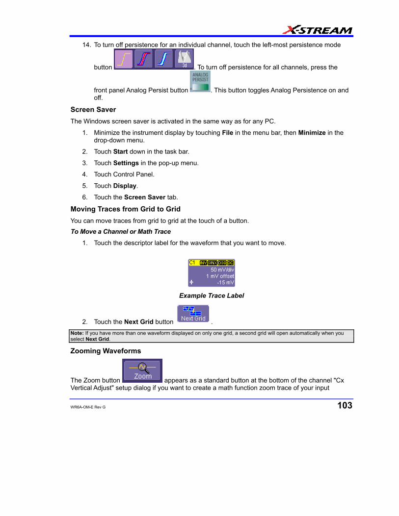
WR6A-OM-E Rev G 103
14. To turn off persistence for an individual channel, touch the left-most persistence mode
button . To turn off persistence for all channels, press the
front panel Analog Persist button . This button toggles Analog Persistence on and off.
Screen Saver The Windows screen saver is activated in the same way as for any PC.
1. Minimize the instrument display by touching File in the menu bar, then Minimize in the drop-down menu.
2. Touch Start down in the task bar.
3. Touch Settings in the pop-up menu.
4. Touch Control Panel.
5. Touch Display.
6. Touch the Screen Saver tab.
Moving Traces from Grid to Grid You can move traces from grid to grid at the touch of a button. To Move a Channel or Math Trace
1. Touch the descriptor label for the waveform that you want to move.
Example Trace Label
2. Touch the Next Grid button . Note: If you have more than one waveform displayed on only one grid, a second grid will open automatically when you select Next Grid.
Zooming Waveforms
The Zoom button appears as a standard button at the bottom of the channel "Cx Vertical Adjust" setup dialog if you want to create a math function zoom trace of your input
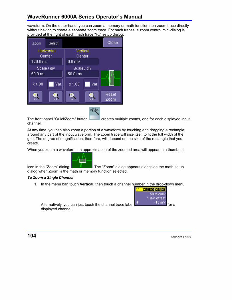
WaveRunner 6000A Series Operator's Manual
104 WR6A-OM-E Rev G
waveform. On the other hand, you can zoom a memory or math function non-zoom trace directly without having to create a separate zoom trace. For such traces, a zoom control mini-dialog is provided at the right of each math trace "Fx" setup dialog:
The front panel "QuickZoom" button creates multiple zooms, one for each displayed input channel.
At any time, you can also zoom a portion of a waveform by touching and dragging a rectangle around any part of the input waveform. The zoom trace will size itself to fit the full width of the grid. The degree of magnification, therefore, will depend on the size of the rectangle that you create.
When you zoom a waveform, an approximation of the zoomed area will appear in a thumbnail
icon in the "Zoom" dialog: . The "Zoom" dialog appears alongside the math setup dialog when Zoom is the math or memory function selected. To Zoom a Single Channel
1. In the menu bar, touch Vertical; then touch a channel number in the drop-down menu.
Alternatively, you can just touch the channel trace label for a displayed channel.

WR6A-OM-E Rev G 105
2. Touch at the bottom of the "Cx Vertical Adjust dialog." A zoom math trace (one of F5 to Fx The number of math traces available depends on the software options loaded on your scope. See specifications.) will be created of the selected channel.
3. To vary the degree of zoom, touch the newly created Fx trace label. The setup dialog for the math function opens, and the zoom control dialog appears at lower-right. It shows the current horizontal and vertical zoom factors.
4. If you want to increase or decrease your horizontal or vertical zoom in small increments, touch the Var. checkbox to enable variable zooming. Now with each touch of the zoom
control buttons , the degree of magnification will change by a small increment. To zoom in or out in large standard increments with each touch of the zoom control buttons, leave the Var. checkbox unchecked. To set exact horizontal or vertical zoom factors, touch inside the Horizontal Scale/div data entry field and enter a time-per-div value, using the pop-up numeric keypad. Then touch inside the Vertical Scale/div field and enter a voltage value.
5. To reset the zoom to x1 magnification, touch Reset Zoom in the dialog or press the front
panel zoom button . To Zoom by Touch-and-Drag
1. Touch and drag a rectangle around any part of an input channel waveform, math trace, or memory trace. If you have more than one trace displayed, a pop-up "Rectangle Zoom Wizard" will appear.
2. If more than one trace is displayed, touch the "Source" tab and select a trace to act on. 3. Touch the "Action" tab and select Create a New Zoom Trace. You will be offered the
choice of creating a new zoom trace or modifying the current trace. 4. Touch the Zoom tab and select a math function trace to display the zoom.
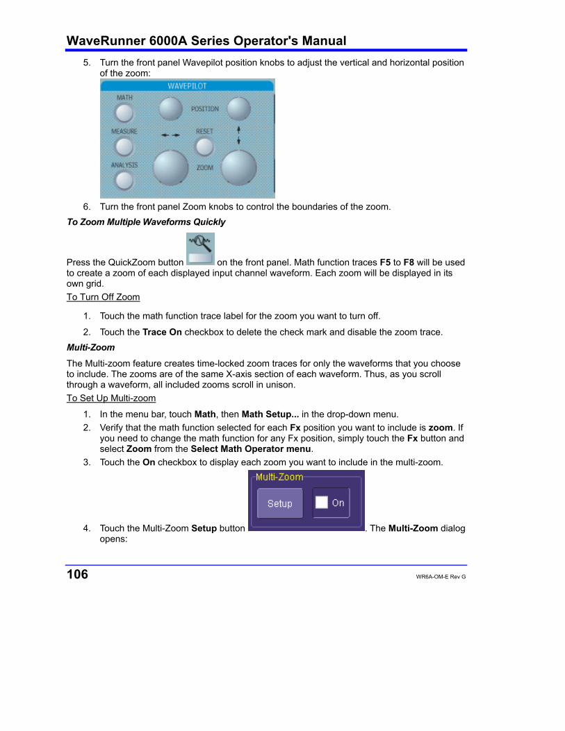
WaveRunner 6000A Series Operator's Manual
106 WR6A-OM-E Rev G
5. Turn the front panel Wavepilot position knobs to adjust the vertical and horizontal position of the zoom:
6. Turn the front panel Zoom knobs to control the boundaries of the zoom.
To Zoom Multiple Waveforms Quickly
Press the QuickZoom button on the front panel. Math function traces F5 to F8 will be used to create a zoom of each displayed input channel waveform. Each zoom will be displayed in its own grid. To Turn Off Zoom
1. Touch the math function trace label for the zoom you want to turn off.
2. Touch the Trace On checkbox to delete the check mark and disable the zoom trace. Multi-Zoom
The Multi-zoom feature creates time-locked zoom traces for only the waveforms that you choose to include. The zooms are of the same X-axis section of each waveform. Thus, as you scroll through a waveform, all included zooms scroll in unison. To Set Up Multi-zoom
1. In the menu bar, touch Math, then Math Setup... in the drop-down menu. 2. Verify that the math function selected for each Fx position you want to include is zoom. If
you need to change the math function for any Fx position, simply touch the Fx button and select Zoom from the Select Math Operator menu.
3. Touch the On checkbox to display each zoom you want to include in the multi-zoom.
4. Touch the Multi-Zoom Setup button . The Multi-Zoom dialog opens:
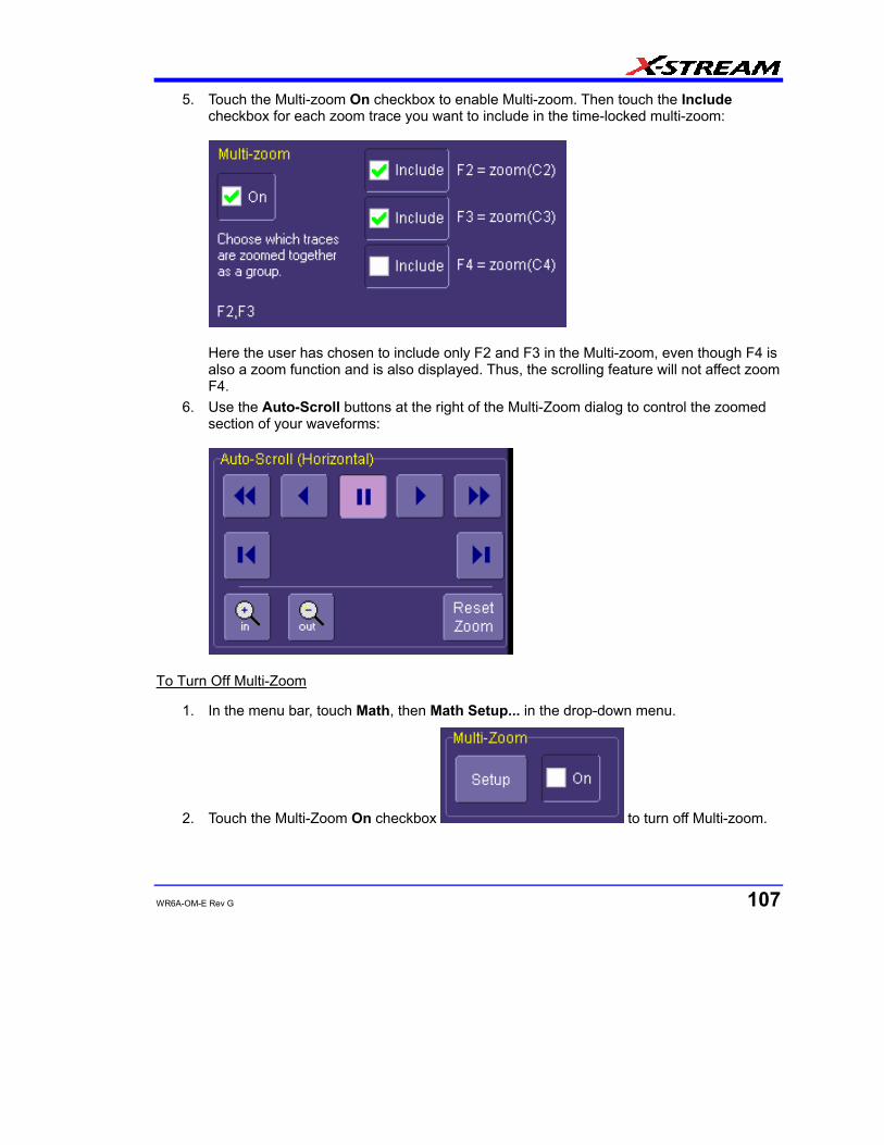
WR6A-OM-E Rev G 107
5. Touch the Multi-zoom On checkbox to enable Multi-zoom. Then touch the Include checkbox for each zoom trace you want to include in the time-locked multi-zoom:
Here the user has chosen to include only F2 and F3 in the Multi-zoom, even though F4 is also a zoom function and is also displayed. Thus, the scrolling feature will not affect zoom F4.
6. Use the Auto-Scroll buttons at the right of the Multi-Zoom dialog to control the zoomed section of your waveforms:
To Turn Off Multi-Zoom
1. In the menu bar, touch Math, then Math Setup... in the drop-down menu.
2. Touch the Multi-Zoom On checkbox to turn off Multi-zoom.
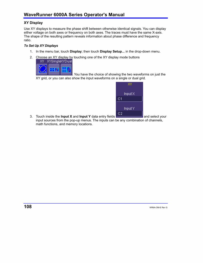
WaveRunner 6000A Series Operator's Manual
108 WR6A-OM-E Rev G
XY Display Use XY displays to measure the phase shift between otherwise identical signals. You can display either voltage on both axes or frequency on both axes. The traces must have the same X-axis. The shape of the resulting pattern reveals information about phase difference and frequency ratio. To Set Up XY Displays
1. In the menu bar, touch Display; then touch Display Setup... in the drop-down menu.
2. Choose an XY display by touching one of the XY display mode buttons
. You have the choice of showing the two waveforms on just the XY grid, or you can also show the input waveforms on a single or dual grid.
3. Touch inside the Input X and Input Y data entry fields and select your input sources from the pop-up menus. The inputs can be any combination of channels, math functions, and memory locations.
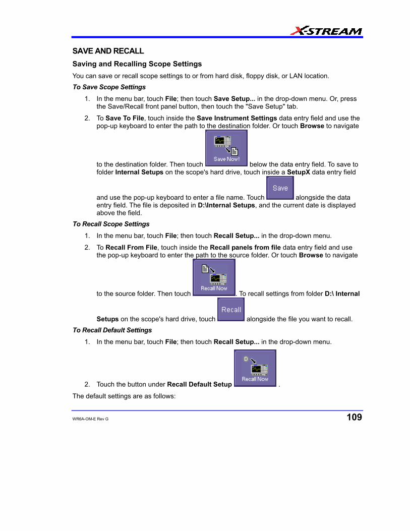
WR6A-OM-E Rev G 109
SAVE AND RECALL Saving and Recalling Scope Settings You can save or recall scope settings to or from hard disk, floppy disk, or LAN location. To Save Scope Settings
1. In the menu bar, touch File; then touch Save Setup... in the drop-down menu. Or, press the Save/Recall front panel button, then touch the "Save Setup" tab.
2. To Save To File, touch inside the Save Instrument Settings data entry field and use the pop-up keyboard to enter the path to the destination folder. Or touch Browse to navigate
to the destination folder. Then touch below the data entry field. To save to folder Internal Setups on the scope's hard drive, touch inside a SetupX data entry field
and use the pop-up keyboard to enter a file name. Touch alongside the data entry field. The file is deposited in D:\Internal Setups, and the current date is displayed above the field.
To Recall Scope Settings
1. In the menu bar, touch File; then touch Recall Setup... in the drop-down menu.
2. To Recall From File, touch inside the Recall panels from file data entry field and use the pop-up keyboard to enter the path to the source folder. Or touch Browse to navigate
to the source folder. Then touch . To recall settings from folder D:\ Internal
Setups on the scope's hard drive, touch alongside the file you want to recall. To Recall Default Settings
1. In the menu bar, touch File; then touch Recall Setup... in the drop-down menu.
2. Touch the button under Recall Default Setup .
The default settings are as follows:
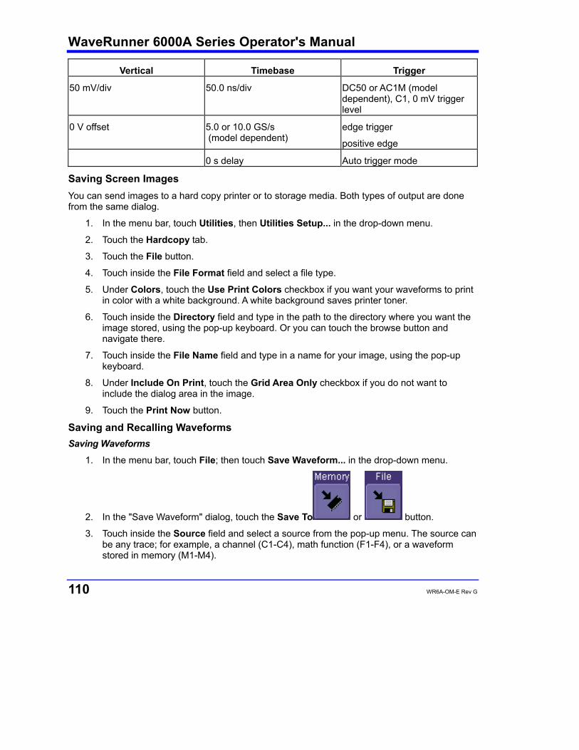
WaveRunner 6000A Series Operator's Manual
110 WR6A-OM-E Rev G
Vertical Timebase Trigger
50 mV/div 50.0 ns/div DC50 or AC1M (model dependent), C1, 0 mV trigger level
0 V offset 5.0 or 10.0 GS/s (model dependent)
edge trigger
positive edge
0 s delay Auto trigger mode
Saving Screen Images You can send images to a hard copy printer or to storage media. Both types of output are done from the same dialog.
1. In the menu bar, touch Utilities, then Utilities Setup... in the drop-down menu.
2. Touch the Hardcopy tab.
3. Touch the File button.
4. Touch inside the File Format field and select a file type.
5. Under Colors, touch the Use Print Colors checkbox if you want your waveforms to print in color with a white background. A white background saves printer toner.
6. Touch inside the Directory field and type in the path to the directory where you want the image stored, using the pop-up keyboard. Or you can touch the browse button and navigate there.
7. Touch inside the File Name field and type in a name for your image, using the pop-up keyboard.
8. Under Include On Print, touch the Grid Area Only checkbox if you do not want to include the dialog area in the image.
9. Touch the Print Now button.
Saving and Recalling Waveforms Saving Waveforms
1. In the menu bar, touch File; then touch Save Waveform... in the drop-down menu.
2. In the "Save Waveform" dialog, touch the Save To or button.
3. Touch inside the Source field and select a source from the pop-up menu. The source can be any trace; for example, a channel (C1-C4), math function (F1-F4), or a waveform stored in memory (M1-M4).
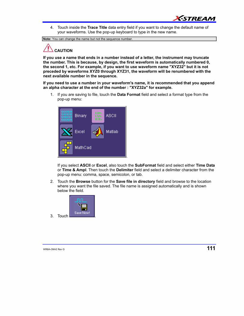
WR6A-OM-E Rev G 111
4. Touch inside the Trace Title data entry field if you want to change the default name of your waveforms. Use the pop-up keyboard to type in the new name.
Note: You can change the name but not the sequence number.
CAUTION
If you use a name that ends in a number instead of a letter, the instrument may truncate the number. This is because, by design, the first waveform is automatically numbered 0, the second 1, etc. For example, if you want to use waveform name "XYZ32" but it is not preceded by waveforms XYZ0 through XYZ31, the waveform will be renumbered with the next available number in the sequence.
If you need to use a number in your waveform's name, it is recommended that you append an alpha character at the end of the number : "XYZ32a" for example.
1. If you are saving to file, touch the Data Format field and select a format type from the pop-up menu:
. If you select ASCII or Excel, also touch the SubFormat field and select either Time Data or Time & Ampl. Then touch the Delimiter field and select a delimiter character from the pop-up menu: comma, space, semicolon, or tab.
2. Touch the Browse button for the Save file in directory field and browse to the location where you want the file saved. The file name is assigned automatically and is shown below the field.
3. Touch .
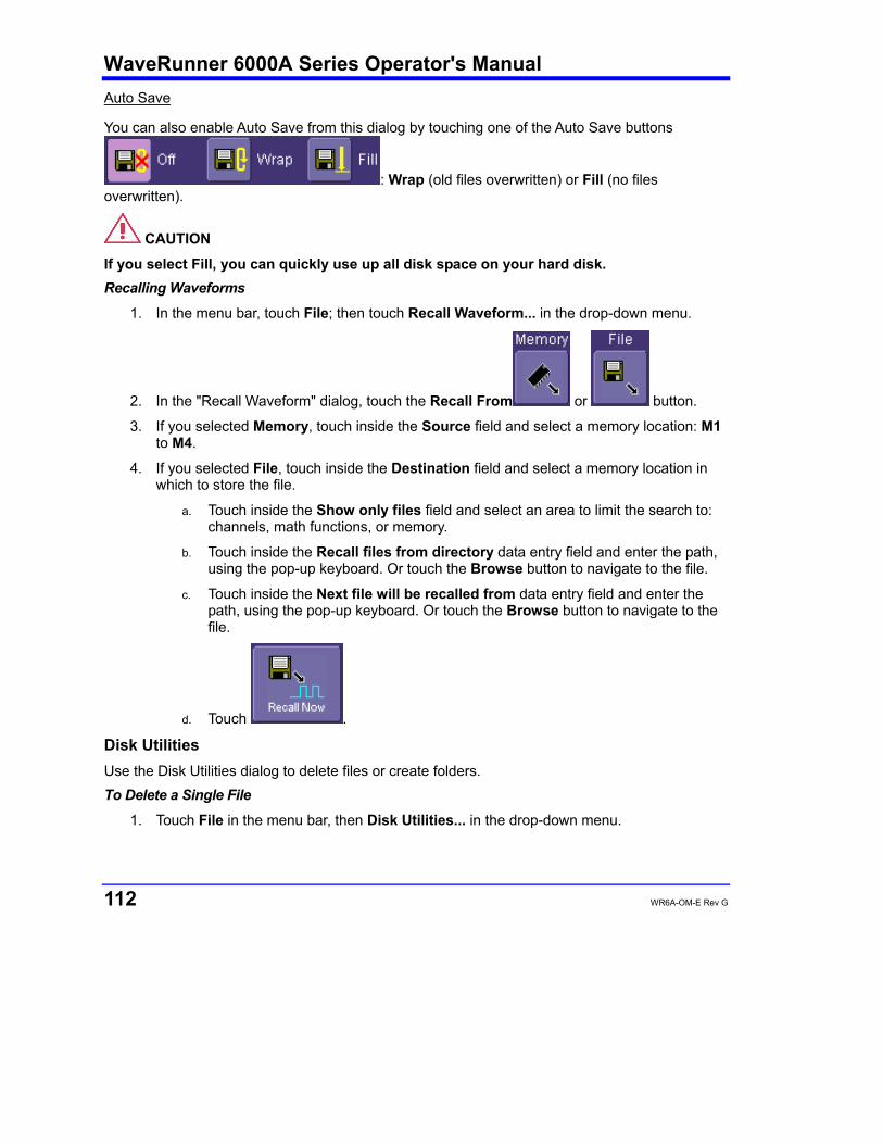
WaveRunner 6000A Series Operator's Manual
112 WR6A-OM-E Rev G
Auto Save
You can also enable Auto Save from this dialog by touching one of the Auto Save buttons
: Wrap (old files overwritten) or Fill (no files overwritten).
CAUTION
If you select Fill, you can quickly use up all disk space on your hard disk. Recalling Waveforms
1. In the menu bar, touch File; then touch Recall Waveform... in the drop-down menu.
2. In the "Recall Waveform" dialog, touch the Recall From or button.
3. If you selected Memory, touch inside the Source field and select a memory location: M1 to M4.
4. If you selected File, touch inside the Destination field and select a memory location in which to store the file.
a. Touch inside the Show only files field and select an area to limit the search to: channels, math functions, or memory.
b. Touch inside the Recall files from directory data entry field and enter the path, using the pop-up keyboard. Or touch the Browse button to navigate to the file.
c. Touch inside the Next file will be recalled from data entry field and enter the path, using the pop-up keyboard. Or touch the Browse button to navigate to the file.
d. Touch .
Disk Utilities Use the Disk Utilities dialog to delete files or create folders. To Delete a Single File
1. Touch File in the menu bar, then Disk Utilities... in the drop-down menu.
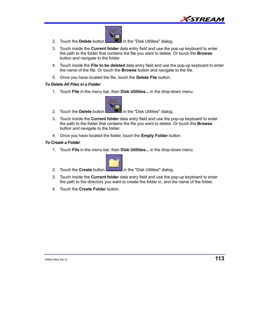
WR6A-OM-E Rev G 113
2. Touch the Delete button in the "Disk Utilities" dialog.
3. Touch inside the Current folder data entry field and use the pop-up keyboard to enter the path to the folder that contains the file you want to delete. Or touch the Browse button and navigate to the folder.
4. Touch inside the File to be deleted data entry field and use the pop-up keyboard to enter the name of the file. Or touch the Browse button and navigate to the file.
5. Once you have located the file, touch the Delete File button. To Delete All Files in a Folder
1. Touch File in the menu bar, then Disk Utilities... in the drop-down menu.
2. Touch the Delete button in the "Disk Utilities" dialog.
3. Touch inside the Current folder data entry field and use the pop-up keyboard to enter the path to the folder that contains the file you want to delete. Or touch the Browse button and navigate to the folder.
4. Once you have located the folder, touch the Empty Folder button. To Create a Folder
1. Touch File in the menu bar, then Disk Utilities... in the drop-down menu.
2. Touch the Create button in the "Disk Utilities" dialog.
3. Touch inside the Current folder data entry field and use the pop-up keyboard to enter the path to the directory you want to create the folder in, and the name of the folder.
4. Touch the Create Folder button.
WaveRunner 6000A Series Operator's Manual
114 WR6A-OM-E Rev G
PRINTING AND FILE MANAGEMENT Print, Plot, or Copy The instrument gives you the ability to output files to a printer or plotter, to print to file, or to e-mail your files. Any Windows 2000 supported printer is supported by your instrument.
Printing To Set Up the Printer
1. In the menu bar, touch File, then Print Setup... in the drop-down menu. The Utilities Hardcopy dialog opens.
2. In the dialog area, touch the Printer icon .
3. Under Colors, touch the Use Print Colors checkbox if you want the traces printed on a white background. A white background saves printer toner. (You can change the printer colors in the Preference dialog;)
4. Touch inside the Select Printer field. From the touch pad pop-up choose the printer you want to print to. Touch the Properties button to see your printer setup.
5. Touch the icon for the layout Orientation you want: portrait or landscape.
6. Touch the Grid Area Only checkbox if you do not need to print the dialog area and you only want to show the waveforms and grids.
To Print
1. You can print in one of three ways:
2. Press the printer button on the front panel:
3. In the menu bar, touch File, then Print in the drop-down menu.
4. Touch the Print Now button in the "Hardcopy" dialog Adding Printers and Drivers Note: If you want to add a printer driver, the driver must first be loaded on the scope.
1. In the menu bar, touch File, then Print Setup... in the drop-down menu. The Utilities Hardcopy dialog opens.
2. In the dialog area, touch the Printer icon .
3. Touch the Add Printer button. An MS Windows® window with which to add a printer will open.
4. Touch the Properties button to change printer properties such as number of copies.

WR6A-OM-E Rev G 115
Changing the Default Printer
1. If you want to change the default printer, minimize the instrument application by touching File in the menu bar, then Minimize in the drop-down menu.
2. Touch the Start button in the task bar at the bottom of the screen.
3. Select Settings, then Printers.
4. Touch the printer you want to set as the default printer, then touch File, Set as Default Printer.
Managing Files Use the instrument's utilities to create waveform files on floppy disk, internal hard drive or network drives. You can copy files from your hard drive to floppy disk. You also can give your files custom names and create directories for them. Hard Disk Partitions
The instrument's hard disk is partitioned into drive C: and drive D:. Drive C: contains the Windows operating system and the instrument application software. Drive D: is intended for data files.
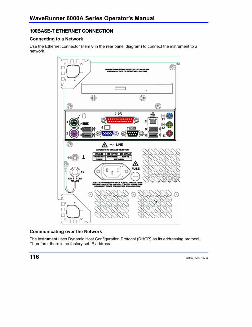
WaveRunner 6000A Series Operator's Manual
116 WR6A-OM-E Rev G
100BASE-T ETHERNET CONNECTION Connecting to a Network Use the Ethernet connector (item 8 in the rear panel diagram) to connect the instrument to a network.
Communicating over the Network The instrument uses Dynamic Host Configuration Protocol (DHCP) as its addressing protocol. Therefore, there is no factory set IP address.
WR6A-OM-E Rev G 117
Windows Setups
If the instrument is to reside within a domain on your LAN, your IS administrator will have to connect the DSO.
Guidelines for Working in Windows
Although the instrument has an open architecture, avoid modifying the Windows operating system, since this may cause problems for the instrument's user interface. Please follow these recommendations:
• Do not load any version of Windows not provided by LeCroy. If you load any Windows 2000 service packs from Microsoft, please be advised that LeCroy cannot guarantee trouble-free operation afterwards.
• Avoid modifying Control Panel settings.
• Do not change the color resolution (24 bit) or screen size (800 x 600 pixel) settings.
• After you load third-party software applications, if your scope does not work properly try reloading the instrument software from the CD shipped with the scope.
• Do not modify or remove any system fonts; doing so may affect the readability of the dialogs.
• Do not change any display properties like Background, Appearance, Effects, or Settings. Functionality of the scope or screen saver may be affected.
• Do not make any changes to the Windows folder.
• Do not make any changes to the BIOS settings.
• Do not make any changes to the Windows power management system. Windows Repair Disk
Before you install any hardware or software on your instrument, LeCroy strongly recommends that you create an Emergency Repair Disk. During a system rebuild, the repair process relies on information that is saved in the systemroot\repair folder. You must not change or delete this folder.
You only need a blank 1.44 MB floppy disk to create an Emergency Repair Disk (ERD).
To create an Emergency Repair Disk
1. In the task bar at the bottom of the screen, touch Start, Programs, Accessories, System Tools, Backup.
2. In the "Tools" menu, touch Emergency Repair Disk.
3. Follow the instructions displayed on the screen.

WaveRunner 6000A Series Operator's Manual
118 WR6A-OM-E Rev G
TRACK VIEWS Creating and Viewing a Trend
1. In the menu bar, touch Measure, then Measure Setup in the drop-down menu.
2. Touch one of parameter tabs P1 through Px.
3. Touch inside the Source1 data entry field and select an input waveform from the pop-up menu.
4. Touch inside the Measure data entry field and select a parameter from the pop-up menu.
5. Touch the Trend button at the bottom of the dialog; then, from the Math selection for Trend menu, select a math function location (F1 to Fx The number of math traces available depends on the software options loaded on your scope. See specifications.) to store the Trend display. The Trend will be displayed along with the
trace label Example Trend Trace Label for the math function you selected.
6. Touch the newly displayed Trend math function trace label if you want to change any settings in the Trend dialog:

WR6A-OM-E Rev G 119
Creating a Track View 1. This feature is available in the XMAP option.
2. In the menu bar, touch Measure, then Measure Setup in the drop-down menu.
3. Touch one of parameter tabs P1 through Px.
4. Touch inside the Source1 data entry field and select an input waveform from the pop-up menu.
5. Touch inside the Measure data entry field and select a parameter from the pop-up menu.
6. Touch the Track button at the bottom of the dialog; then, from the Math selection for Track menu, select a math function location (F1 to Fx The number of math traces available depends on the software options loaded on your scope. See specifications.) to store the Track display. The Track will be displayed along with the trace
label Example Track Trace Label for the math function you selected.
7. Touch the newly displayed Track math function trace label if you want to change any settings in the Track dialog:
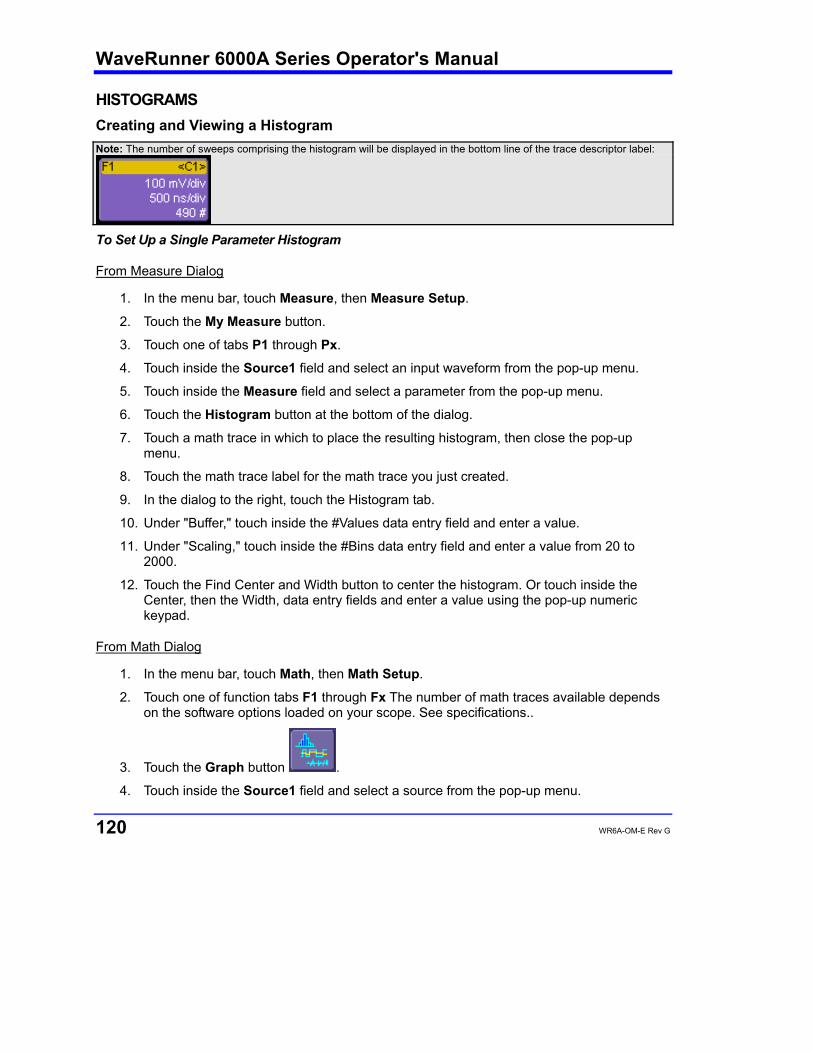
WaveRunner 6000A Series Operator's Manual
120 WR6A-OM-E Rev G
HISTOGRAMS Creating and Viewing a Histogram Note: The number of sweeps comprising the histogram will be displayed in the bottom line of the trace descriptor label:
To Set Up a Single Parameter Histogram
From Measure Dialog
1. In the menu bar, touch Measure, then Measure Setup.
2. Touch the My Measure button.
3. Touch one of tabs P1 through Px.
4. Touch inside the Source1 field and select an input waveform from the pop-up menu.
5. Touch inside the Measure field and select a parameter from the pop-up menu.
6. Touch the Histogram button at the bottom of the dialog.
7. Touch a math trace in which to place the resulting histogram, then close the pop-up menu.
8. Touch the math trace label for the math trace you just created.
9. In the dialog to the right, touch the Histogram tab.
10. Under "Buffer," touch inside the #Values data entry field and enter a value.
11. Under "Scaling," touch inside the #Bins data entry field and enter a value from 20 to 2000.
12. Touch the Find Center and Width button to center the histogram. Or touch inside the Center, then the Width, data entry fields and enter a value using the pop-up numeric keypad.
From Math Dialog
1. In the menu bar, touch Math, then Math Setup.
2. Touch one of function tabs F1 through Fx The number of math traces available depends on the software options loaded on your scope. See specifications..
3. Touch the Graph button .
4. Touch inside the Source1 field and select a source from the pop-up menu.
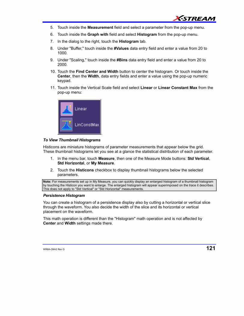
WR6A-OM-E Rev G 121
5. Touch inside the Measurement field and select a parameter from the pop-up menu.
6. Touch inside the Graph with field and select Histogram from the pop-up menu.
7. In the dialog to the right, touch the Histogram tab.
8. Under "Buffer," touch inside the #Values data entry field and enter a value from 20 to 1000.
9. Under "Scaling," touch inside the #Bins data entry field and enter a value from 20 to 2000.
10. Touch the Find Center and Width button to center the histogram. Or touch inside the Center, then the Width, data entry fields and enter a value using the pop-up numeric keypad.
11. Touch inside the Vertical Scale field and select Linear or Linear Constant Max from the pop-up menu:
. To View Thumbnail Histograms
Histicons are miniature histograms of parameter measurements that appear below the grid. These thumbnail histograms let you see at a glance the statistical distribution of each parameter.
1. In the menu bar, touch Measure, then one of the Measure Mode buttons: Std Vertical, Std Horizontal, or My Measure.
2. Touch the Histicons checkbox to display thumbnail histograms below the selected parameters.
Note: For measurements set up in My Measure, you can quickly display an enlarged histogram of a thumbnail histogram by touching the Histicon you want to enlarge. The enlarged histogram will appear superimposed on the trace it describes. This does not apply to "Std Vertical" or "Std Horizontal" measurements.
Persistence Histogram
You can create a histogram of a persistence display also by cutting a horizontal or vertical slice through the waveform. You also decide the width of the slice and its horizontal or vertical placement on the waveform.
This math operation is different than the "Histogram" math operation and is not affected by Center and Width settings made there.

WaveRunner 6000A Series Operator's Manual
122 WR6A-OM-E Rev G
To Set Up Persistence Histograms
1. In the menu bar, touch Math, then Math Setup.
2. Touch one of function tabs F1 through Fx The number of math traces available depends on the software options loaded on your scope. See specifications..
3. Touch inside the Source1 field and select a source from the pop-up menu.
4. Touch inside the Operator1 field and select Phistogram from the Select Math Operator menu.
5. Touch the "Phistogram" tab, then touch inside the Slice Direction field and select Horizontal or Vertical slice from the pop-up menu.
6. Touch inside the Slice Center field and enter a value, using the pop-up keypad.
7. Touch inside the Slice Width field and enter a value, using the pop-up keypad. Note: You can use the front panel Adjust knobs to move the Slice Center line and the Slice Width boundary lines.
Persistence Trace Range
This math operation has a field where you can enter the percent of the persistence trace population to use in creating a new waveform. Persistence Sigma
This math operation has a field where you can enter a scale, measured in standard deviations, by which to create a new waveform.
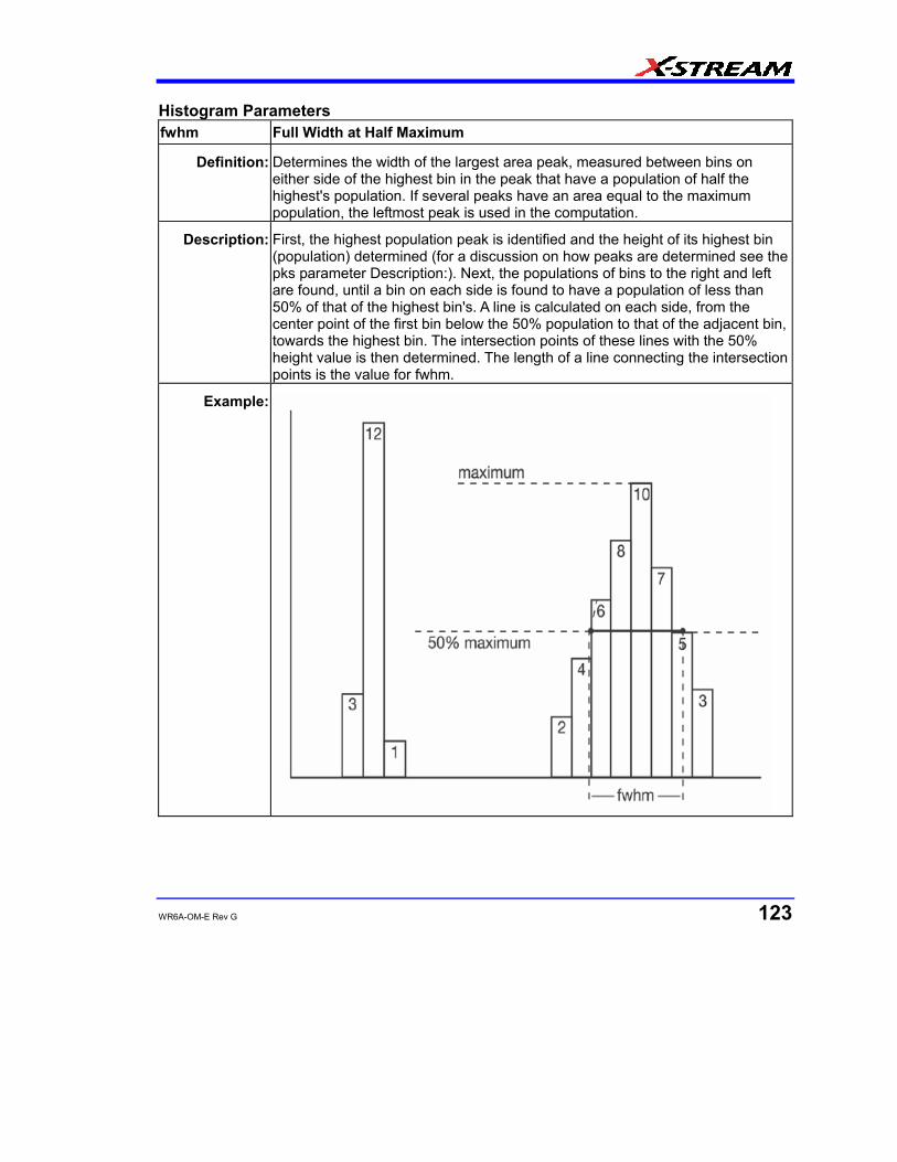
WR6A-OM-E Rev G 123
Histogram Parameters fwhm Full Width at Half Maximum
Definition: Determines the width of the largest area peak, measured between bins on either side of the highest bin in the peak that have a population of half the highest's population. If several peaks have an area equal to the maximum population, the leftmost peak is used in the computation.
Description: First, the highest population peak is identified and the height of its highest bin (population) determined (for a discussion on how peaks are determined see the pks parameter Description:). Next, the populations of bins to the right and left are found, until a bin on each side is found to have a population of less than 50% of that of the highest bin's. A line is calculated on each side, from the center point of the first bin below the 50% population to that of the adjacent bin, towards the highest bin. The intersection points of these lines with the 50% height value is then determined. The length of a line connecting the intersection points is the value for fwhm.
Example:
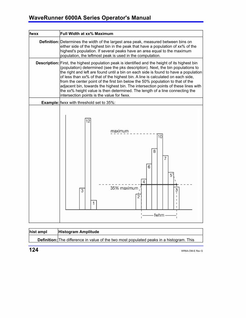
WaveRunner 6000A Series Operator's Manual
124 WR6A-OM-E Rev G
fwxx Full Width at xx% Maximum
Definition: Determines the width of the largest area peak, measured between bins on either side of the highest bin in the peak that have a population of xx% of the highest's population. If several peaks have an area equal to the maximum population, the leftmost peak is used in the computation.
Description: First, the highest population peak is identified and the height of its highest bin (population) determined (see the pks description). Next, the bin populations to the right and left are found until a bin on each side is found to have a population of less than xx% of that of the highest bin. A line is calculated on each side, from the center point of the first bin below the 50% population to that of the adjacent bin, towards the highest bin. The intersection points of these lines with the xx% height value is then determined. The length of a line connecting the intersection points is the value for fwxx.
Example: fwxx with threshold set to 35%:
hist ampl Histogram Amplitude
Definition: The difference in value of the two most populated peaks in a histogram. This

WR6A-OM-E Rev G 125
parameter is useful for waveforms with two primary parameter values, such as TTL voltages, where hampl would indicate the difference between the binary `1' and `0' voltage values.
Description: The values at the center (line dividing the population of peak in half) of the two highest peaks are determined (see pks parameter description:). The value of the leftmost of the two peaks is the histogram base (see hbase). While that of the rightmost is the histogram top (see htop). The parameter is then calculated as:
hampl = htop hbase
Example:
In this histogram, hampl is 152 mV 150 mV = 2 mV.
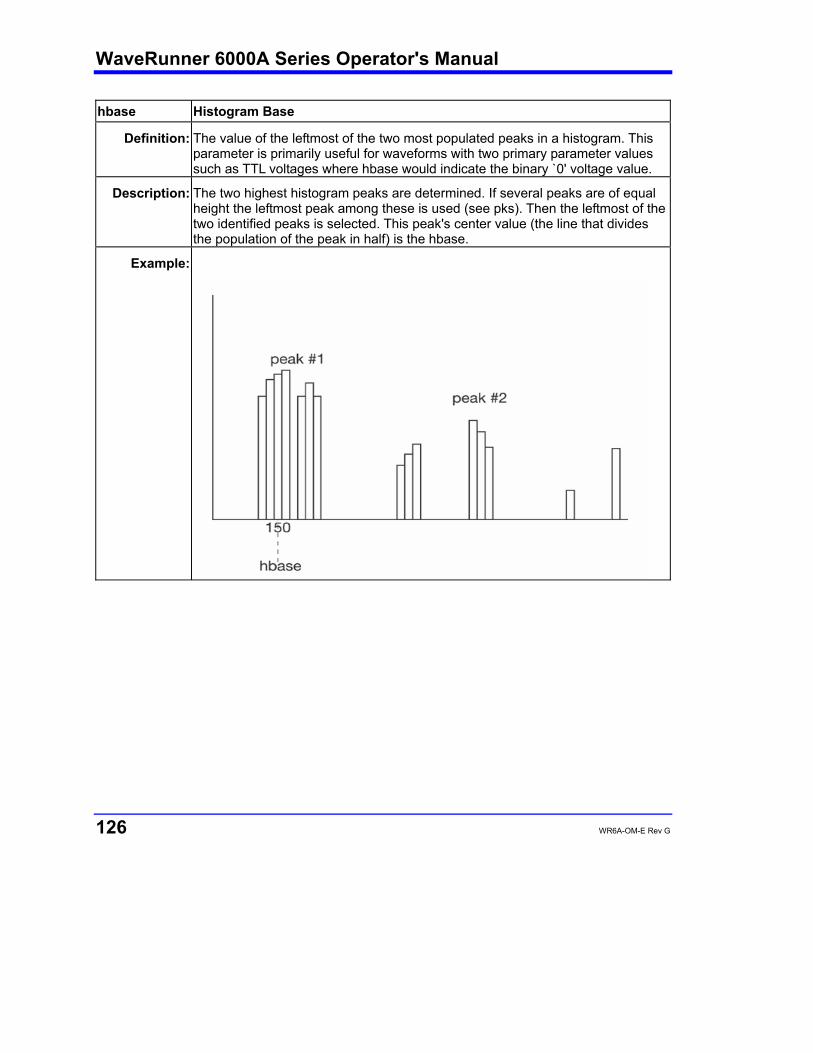
WaveRunner 6000A Series Operator's Manual
126 WR6A-OM-E Rev G
hbase Histogram Base
Definition: The value of the leftmost of the two most populated peaks in a histogram. This parameter is primarily useful for waveforms with two primary parameter values such as TTL voltages where hbase would indicate the binary `0' voltage value.
Description: The two highest histogram peaks are determined. If several peaks are of equal height the leftmost peak among these is used (see pks). Then the leftmost of the two identified peaks is selected. This peak's center value (the line that divides the population of the peak in half) is the hbase.
Example:
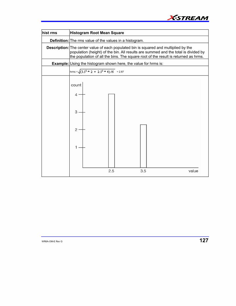
WR6A-OM-E Rev G 127
hist rms Histogram Root Mean Square
Definition: The rms value of the values in a histogram.
Description: The center value of each populated bin is squared and multiplied by the population (height) of the bin. All results are summed and the total is divided by the population of all the bins. The square root of the result is returned as hrms.
Example: Using the histogram shown here, the value for hrms is:
hrms = = 2.87
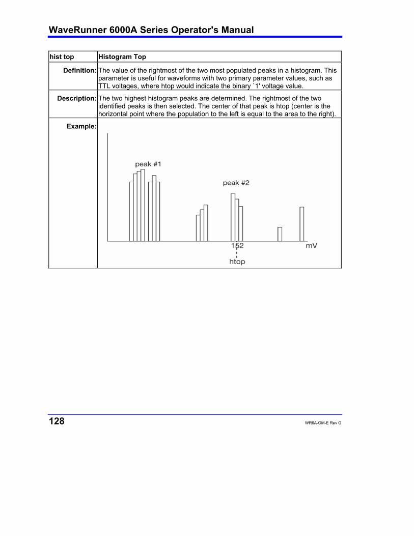
WaveRunner 6000A Series Operator's Manual
128 WR6A-OM-E Rev G
hist top Histogram Top
Definition: The value of the rightmost of the two most populated peaks in a histogram. This parameter is useful for waveforms with two primary parameter values, such as TTL voltages, where htop would indicate the binary `1' voltage value.
Description: The two highest histogram peaks are determined. The rightmost of the two identified peaks is then selected. The center of that peak is htop (center is the horizontal point where the population to the left is equal to the area to the right).
Example:
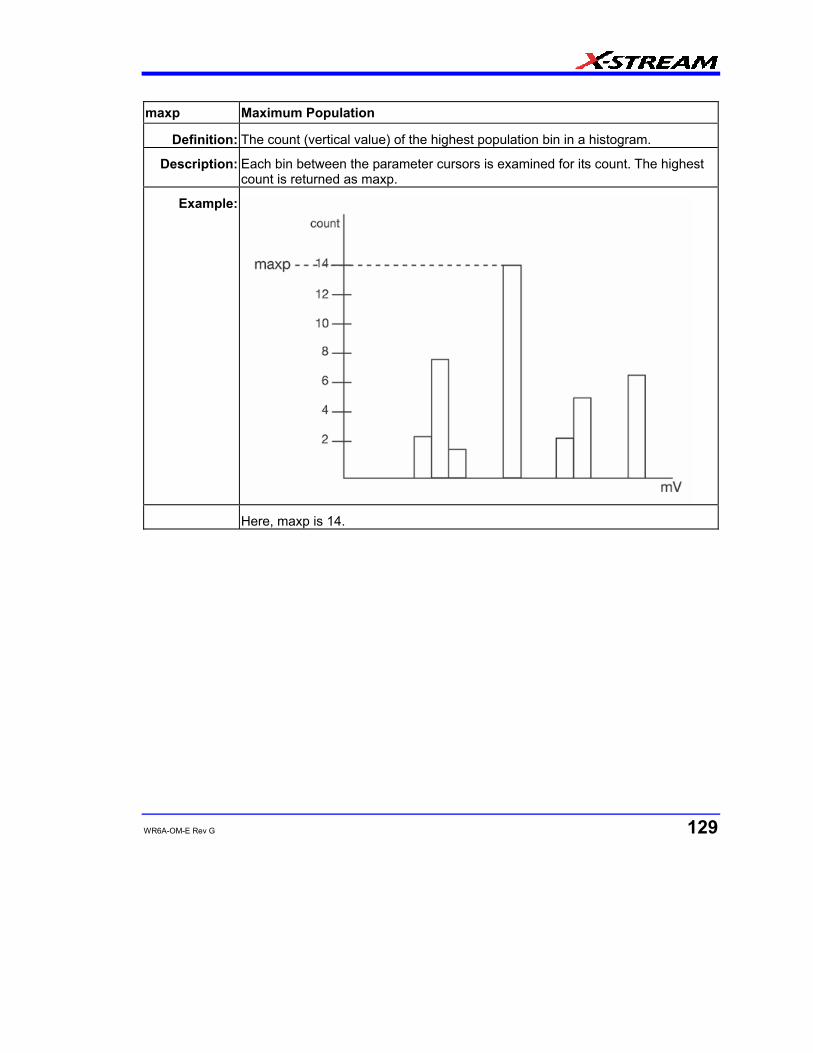
WR6A-OM-E Rev G 129
maxp Maximum Population
Definition: The count (vertical value) of the highest population bin in a histogram.
Description: Each bin between the parameter cursors is examined for its count. The highest count is returned as maxp.
Example:
Here, maxp is 14.
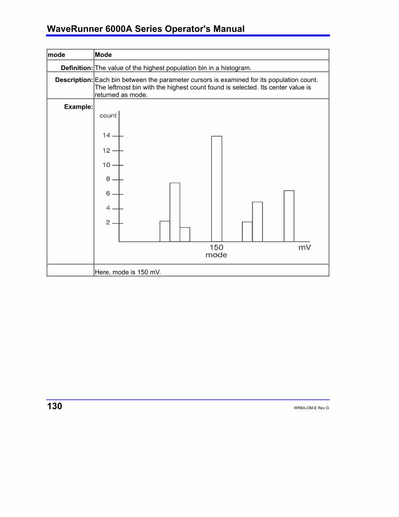
WaveRunner 6000A Series Operator's Manual
130 WR6A-OM-E Rev G
mode Mode
Definition: The value of the highest population bin in a histogram.
Description: Each bin between the parameter cursors is examined for its population count. The leftmost bin with the highest count found is selected. Its center value is returned as mode.
Example:
Here, mode is 150 mV.

WR6A-OM-E Rev G 131
pctl Percentile
Definition: Computes the horizontal data value that separates the data in a histogram such that the population on the left is a specified percentage `xx' of the total population. When the threshold is set to 50%, pctl is the same as hmedian.
Description: The total population of the histogram is determined. Scanning from left to right, the population of each bin is summed until a bin that causes the sum to equal or exceed `xx'% of the population value is encountered. A ratio of the number of counts needed for `xx'% population/total bin population is then determined for the bin. The horizontal value of the bin at that ratio point of its range is found, and returned as pctl.
Example: The total population of a histogram is 100. The histogram range is divided into 20 bins and `xx' is set to 25%. The population sum at the sixth bin from the left is 22. The population of the seventh is 9 and its sub-range is 6.1 to 6.4 V. The ratio of counts needed for 25% population to total bin population is:
3 counts needed / 9 counts = 1/3.
The value for pctl is:
6.1 volts + .33 * (6.4 6.1) volts = 6.2 volts.
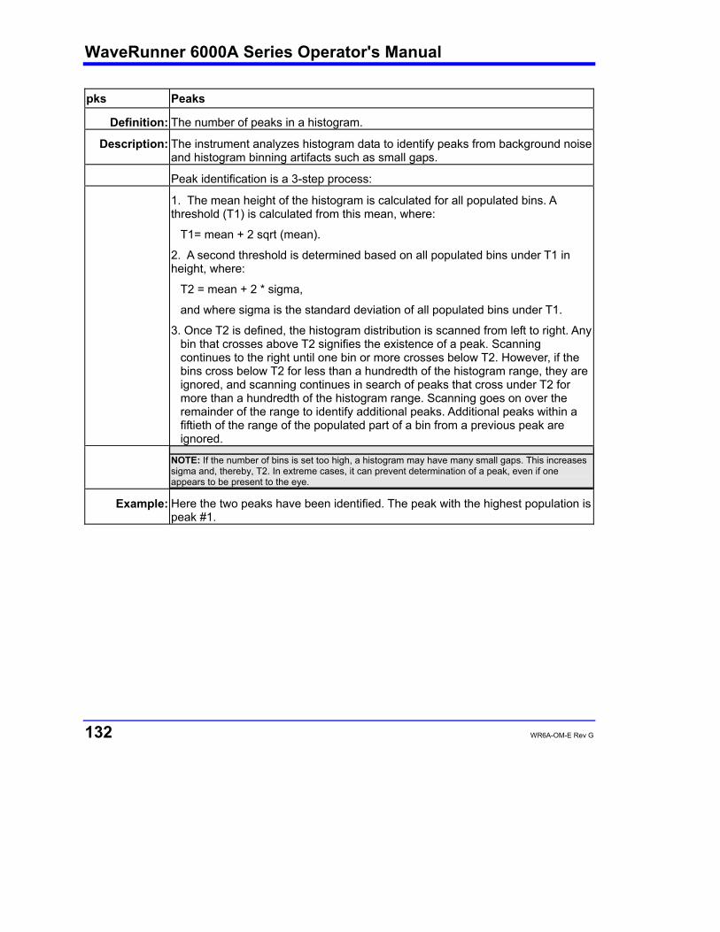
WaveRunner 6000A Series Operator's Manual
132 WR6A-OM-E Rev G
pks Peaks
Definition: The number of peaks in a histogram.
Description: The instrument analyzes histogram data to identify peaks from background noise and histogram binning artifacts such as small gaps.
Peak identification is a 3-step process:
1. The mean height of the histogram is calculated for all populated bins. A threshold (T1) is calculated from this mean, where:
T1= mean + 2 sqrt (mean).
2. A second threshold is determined based on all populated bins under T1 in height, where:
T2 = mean + 2 * sigma,
and where sigma is the standard deviation of all populated bins under T1.
3. Once T2 is defined, the histogram distribution is scanned from left to right. Any bin that crosses above T2 signifies the existence of a peak. Scanning continues to the right until one bin or more crosses below T2. However, if the bins cross below T2 for less than a hundredth of the histogram range, they are ignored, and scanning continues in search of peaks that cross under T2 for more than a hundredth of the histogram range. Scanning goes on over the remainder of the range to identify additional peaks. Additional peaks within a fiftieth of the range of the populated part of a bin from a previous peak are ignored.
NOTE: If the number of bins is set too high, a histogram may have many small gaps. This increases sigma and, thereby, T2. In extreme cases, it can prevent determination of a peak, even if one appears to be present to the eye.
Example: Here the two peaks have been identified. The peak with the highest population is peak #1.

WR6A-OM-E Rev G 133
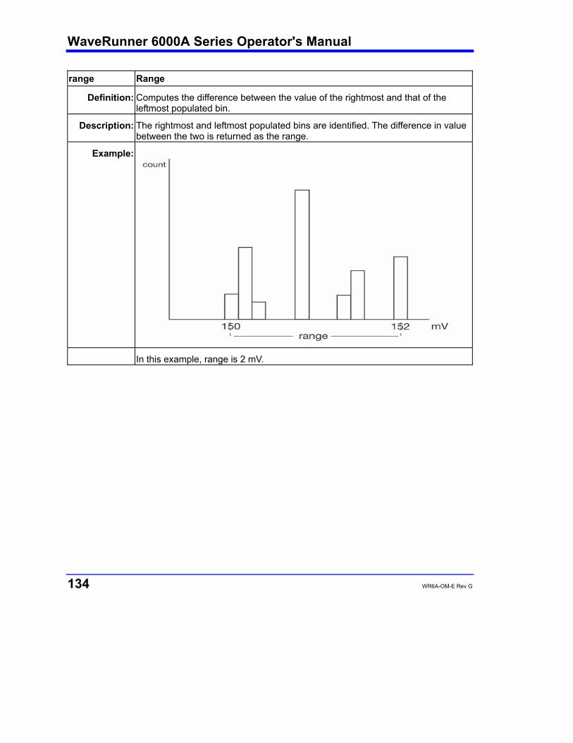
WaveRunner 6000A Series Operator's Manual
134 WR6A-OM-E Rev G
range Range
Definition: Computes the difference between the value of the rightmost and that of the leftmost populated bin.
Description: The rightmost and leftmost populated bins are identified. The difference in value between the two is returned as the range.
Example:
In this example, range is 2 mV.
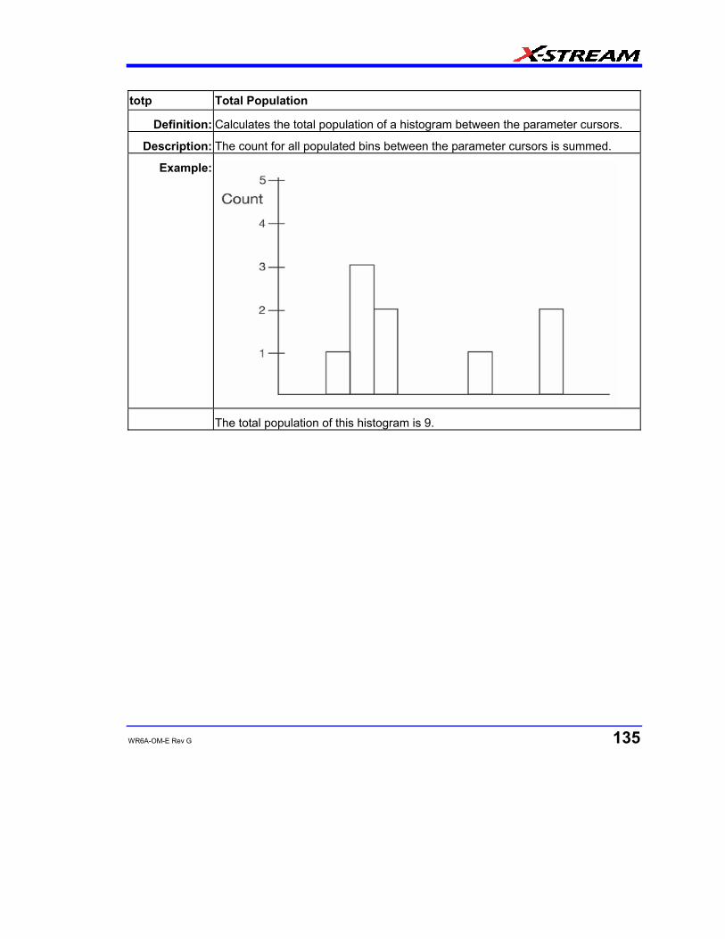
WR6A-OM-E Rev G 135
totp Total Population
Definition: Calculates the total population of a histogram between the parameter cursors.
Description: The count for all populated bins between the parameter cursors is summed.
Example:
The total population of this histogram is 9.
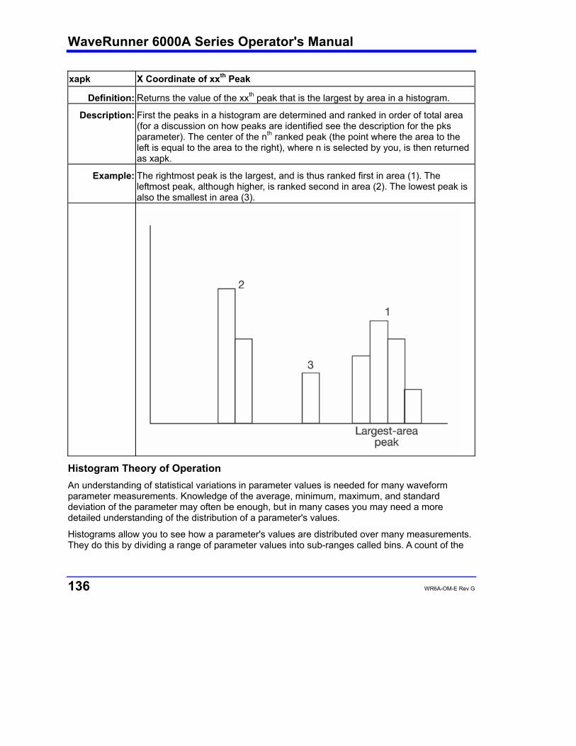
WaveRunner 6000A Series Operator's Manual
136 WR6A-OM-E Rev G
xapk X Coordinate of xxth Peak
Definition: Returns the value of the xxth peak that is the largest by area in a histogram.
Description: First the peaks in a histogram are determined and ranked in order of total area (for a discussion on how peaks are identified see the description for the pks parameter). The center of the nth ranked peak (the point where the area to the left is equal to the area to the right), where n is selected by you, is then returned as xapk.
Example: The rightmost peak is the largest, and is thus ranked first in area (1). The leftmost peak, although higher, is ranked second in area (2). The lowest peak is also the smallest in area (3).
Histogram Theory of Operation An understanding of statistical variations in parameter values is needed for many waveform parameter measurements. Knowledge of the average, minimum, maximum, and standard deviation of the parameter may often be enough, but in many cases you may need a more detailed understanding of the distribution of a parameter's values.
Histograms allow you to see how a parameter's values are distributed over many measurements. They do this by dividing a range of parameter values into sub-ranges called bins. A count of the
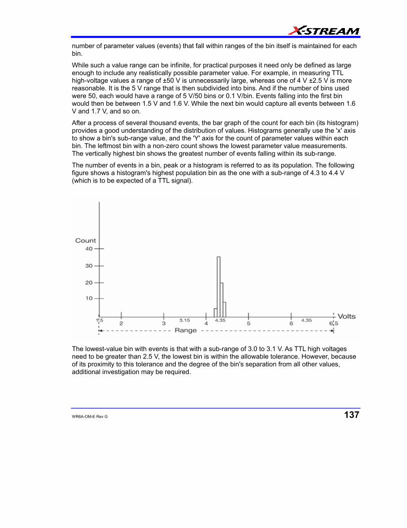
WR6A-OM-E Rev G 137
number of parameter values (events) that fall within ranges of the bin itself is maintained for each bin.
While such a value range can be infinite, for practical purposes it need only be defined as large enough to include any realistically possible parameter value. For example, in measuring TTL high-voltage values a range of ±50 V is unnecessarily large, whereas one of 4 V ±2.5 V is more reasonable. It is the 5 V range that is then subdivided into bins. And if the number of bins used were 50, each would have a range of 5 V/50 bins or 0.1 V/bin. Events falling into the first bin would then be between 1.5 V and 1.6 V. While the next bin would capture all events between 1.6 V and 1.7 V, and so on.
After a process of several thousand events, the bar graph of the count for each bin (its histogram) provides a good understanding of the distribution of values. Histograms generally use the 'x' axis to show a bin's sub-range value, and the 'Y' axis for the count of parameter values within each bin. The leftmost bin with a non-zero count shows the lowest parameter value measurements. The vertically highest bin shows the greatest number of events falling within its sub-range.
The number of events in a bin, peak or a histogram is referred to as its population. The following figure shows a histogram's highest population bin as the one with a sub-range of 4.3 to 4.4 V (which is to be expected of a TTL signal).
The lowest-value bin with events is that with a sub-range of 3.0 to 3.1 V. As TTL high voltages need to be greater than 2.5 V, the lowest bin is within the allowable tolerance. However, because of its proximity to this tolerance and the degree of the bin's separation from all other values, additional investigation may be required.
WaveRunner 6000A Series Operator's Manual
138 WR6A-OM-E Rev G
DSO Process
The instrument generates histograms of the parameter values of input waveforms. But first, you must define the following:
• The parameter to be histogrammed
• The trace on which the histogram is to be displayed
• The maximum number of parameter measurement values to be used in creating the histogram
• The measurement range of the histogram
• The number of bins to be used
Some of these are pre-defined but can be changed. Once they are defined, the oscilloscope is ready to make the histogram. The sequence for acquiring histogram data is as follows:
• Trigger
• Waveform acquisition
• Parameter calculations
• Histogram update
• Trigger re-arm
If you set the timebase for non-segmented mode, a single acquisition occurs prior to parameter calculations. However, in Sequence mode an acquisition for each segment occurs prior to parameter calculations. If the source of histogram data is a memory, saving new data to memory effectively acts as a trigger and acquisition. Because updating the screen can take much processing time, it occurs only once a second, minimizing trigger dead time. Under remote control the display can be turned off to maximize measurement speed. Parameter Buffer
The oscilloscope maintains a circular parameter buffer of the last 20,000 measurements made, including values that fall outside the set histogram range. If the maximum number of events to be used for the histogram is a number `N' less than 20,000, the histogram will be continuously updated with the last `N' events as new acquisitions occur. If the maximum number is greater than 20,000, the histogram will be updated until the number of events is equal to `N.' Then, if the number of bins or the histogram range is modified, the scope will use the parameter buffer values to redraw the histogram with either the last `N' or 20,000 values acquired -- whichever is the lesser. The parameter buffer thereby allows histograms to be redisplayed, using an acquired set of values and settings that produce a distribution shape with the most useful information.
In many cases the optimal range is not readily apparent. So the scope has a powerful range finding function. If required it will examine the values in the parameter buffer to calculate an optimal range and redisplay the histogram using it. The instrument will also give a running count of the number of parameter values that fall within, below, or above the range. If any values fall below or above the range, the range finder can then recalculate to include these parameter values, as long as they are still within the buffer.
WR6A-OM-E Rev G 139
Capture of Parameter Events
The number of events captured per waveform acquisition or display sweep depends on the parameter type. Acquisitions are initiated by the occurrence of a trigger event. Sweeps are equivalent to the waveform captured and displayed on an input channel (1, 2, or 3 or 4). For non-segmented waveforms an acquisition is identical to a sweep. Whereas for segmented waveforms an acquisition occurs for each segment and a sweep is equivalent to acquisitions for all segments. Only the section of a waveform between the parameter cursors is used in the calculation of parameter values and corresponding histogram events.
The following table provides a summary of the number of histogram events captured per acquisition or sweep for each parameter, and for a waveform section between the parameter cursors.
Parameters Number of Events Captured
duty, freq, period, width, time@lev, f@level, f80-20%, fall, r@level, r20-80%, rise
All events in the acquisition
ampl, area, base, cmean, cmedian, crms, csdev, cycles, delay, maximum, mean, minimum, nbph, nbpw, over+, over-, pkpk, npts, rms, sdev, dly
One event per acquisition
Histogram Parameters (XMAP and JTA2 Options) Once a histogram is defined and generated, measurements can be performed on the histogram itself. Typical of these are the histogram's
• average value, standard deviation
• most common value (parameter value of highest count bin)
• leftmost bin position (representing the lowest measured waveform parameter value)
• rightmost bin (representing the highest measured waveform parameter value)
Histogram parameters are provided to enable these measurements. Available through selecting "Statistics" from the "Category" menu, they are calculated for the selected section between the parameter cursors:
fwhm -- full width (of largest peak) at half the maximum bin
fwxx -- full width (of largest peak) at xx% the maximum bin
hist ampl -- histogram amplitude between two largest peaks
hist base -- histogram base or leftmost of two largest peaks
hist max -- value of the highest (right-most) populated bin in a histogram
hist mean -- average or mean value of data in the histogram
hist median -- value of the x-axis of a histogram that divides the population into two equal halves
hist min -- value of the lowest (left-most) populated bin in a histogram
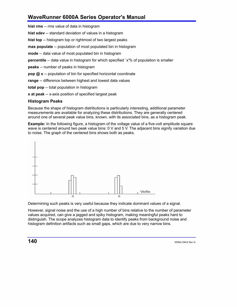
WaveRunner 6000A Series Operator's Manual
140 WR6A-OM-E Rev G
hist rms -- rms value of data in histogram
hist sdev -- standard deviation of values in a histogram
hist top -- histogram top or rightmost of two largest peaks
max populate -- population of most populated bin in histogram
mode -- data value of most populated bin in histogram
percentile -- data value in histogram for which specified `x'% of population is smaller
peaks -- number of peaks in histogram
pop @ x -- population of bin for specified horizontal coordinate
range -- difference between highest and lowest data values
total pop -- total population in histogram
x at peak -- x-axis position of specified largest peak
Histogram Peaks Because the shape of histogram distributions is particularly interesting, additional parameter measurements are available for analyzing these distributions. They are generally centered around one of several peak value bins, known, with its associated bins, as a histogram peak.
Example: In the following figure, a histogram of the voltage value of a five-volt amplitude square wave is centered around two peak value bins: 0 V and 5 V. The adjacent bins signify variation due to noise. The graph of the centered bins shows both as peaks.
Determining such peaks is very useful because they indicate dominant values of a signal.
However, signal noise and the use of a high number of bins relative to the number of parameter values acquired, can give a jagged and spiky histogram, making meaningful peaks hard to distinguish. The scope analyzes histogram data to identify peaks from background noise and histogram definition artifacts such as small gaps, which are due to very narrow bins.
WR6A-OM-E Rev G 141
Binning and Measurement Accuracy Histogram bins represent a sub-range of waveform parameter values, or events. The events represented by a bin may have a value anywhere within its sub-range. However, parameter measurements of the histogram itself, such as average, assume that all events in a bin have a single value. The scope uses the center value of each bin's sub-range in all its calculations. The greater the number of bins used to subdivide a histogram's range, the less the potential deviation between actual event values and those values assumed in histogram parameter calculations.
Nevertheless, using more bins may require that you perform a greater number of waveform parameter measurements, in order to populate the bins sufficiently for the identification of a characteristic histogram distribution.
In addition, very fine grained binning will result in gaps between populated bins that may make it difficult to determine peaks.
The oscilloscope's 20,000-parameter buffer is very effective for determining the optimal number of bins to be used. An optimal bin number is one where the change in parameter values is insignificant, and the histogram distribution does not have a jagged appearance. With this buffer, a histogram can be dynamically redisplayed as the number of bins is modified by the user. In addition, depending on the number of bins selected, the change in waveform parameter values can be seen.

WaveRunner 6000A Series Operator's Manual
142 WR6A-OM-E Rev G
WAVEFORM MEASUREMENTS Measuring with Cursors Cursors are important tools that aid you in measuring signal values. Cursors are markers — lines, cross-hairs, or arrows — that you can move around the grid or the waveform itself. Use cursors to make fast, accurate measurements and to eliminate guesswork. There are two basic types:
Horiz(ontal) (generally Time or Frequency) cursors are markers that you move horizontally along the waveform. Place them at a desired location along the time axis to read the signal’s amplitude at the selected time.
Vert(ical) (Voltage) cursors are lines that you move vertically on the grid to measure the amplitude of a signal. Cursor Measurement Icons
The Readout icons depict what is being measured for each measurement mode.
Each cursor locates a point on the waveform. The cursor values can be read in the descriptor label for the trace. Use the Position data entry fields at the right side of the dialog to place the cursors precisely.
This is the difference in Y values. The value can be read in the descriptor label for the trace.
This gives the slope between cursors.
If there are non-time-domain waveforms displayed, there will also be a menu offering choices of x-axis units: s or Hz, for example.
Cursors Setup Quick Display
At any time, you can change the display of cursor types (or turn them off) without invoking the "Cursors Setup" dialog as follows:
In the menu bar, touch Cursors, then Off, Abs Horizontal, Rel Horizontal, Abs Vertical, or Rel Vertical.
The cursors displayed will assume the positions previously set up. If you want to change their position or measurement mode, in the menu bar touch Cursors, then Cursors Setup in the drop-down menu.
WR6A-OM-E Rev G 143
Full Setup
1. In the menu bar, touch Cursors, then Cursors Setup. The "Standard Cursors" dialog opens.
2. In the dialog area, touch the Cursors On check box to display them.
3. Touch one of the Horizontal or Vertical mode buttons: Relative or Absolute.
4. If you chose a Relative mode, also touch a readout parameter button: Y position, delta Y, or slope.
5. If you chose a Relative mode, touch inside the Position 1 and Position 2 data entry fields and type in a value for each cursor. You can also use the Cursors knobs on the front panel to place the cursors. If you chose an Absolute mode, do the same for your single cursor.
6. If you chose a Relative mode and you would like both cursors to move in unison as you adjust the position, touch the Track check box to enable tracking.
Overview of Parameters Parameters are measurement tools that determine a wide range of waveform properties. Use them to automatically calculate many attributes of your waveform, like rise-time, rms voltage, and peak-to-peak voltage, for example.
There are parameter modes for the amplitude and time domains, custom parameter groups, and parameters for pass and fail testing. You can make common measurements on one or more waveforms. To Turn On Parameters
1. Touch Measure in the menu bar, then Measure Setup... in the drop-down menu.
2. Touch inside the On checkbox for each parameter you want to display. Quick Access to Parameter Setup Dialogs
You can quickly gain access to a parameter setup dialog by touching the parameter list box below the grid. For example, touching within P1 below the grid
displays the setup dialog for P1:

WaveRunner 6000A Series Operator's Manual
144 WR6A-OM-E Rev G
Touching the row titles displays the top Measure dialog. Status Symbols
Below each parameter appears a symbol that indicates the status of the parameter, as follows:
A green check mark means that the scope is returning a valid value.
A crossed-out pulse means that the scope is unable to determine top and base; however, the measurement could still be valid.
A downward pointing arrow indicates an underflow condition.
An upward pointing arrow indicates an overflow condition.
An upward-and-downward pointing arrow indicates an underflow and overflow condition.

WR6A-OM-E Rev G 145
Using X-Stream Browser to Obtain Status Information
Example:
Here is a case of an overflow condition, in which the amplitude of the waveform cannot be determined:
1. Minimize the scope display by selecting File Minimize.
2. Touch the X-Stream Browser desktop icon to open the browser.
3. Touch the left scope icon ("Connect to a local X-Stream DSO device") in the X-Stream Browser toolbar:
4. Select Measure Parameter in error (P1) Out Result
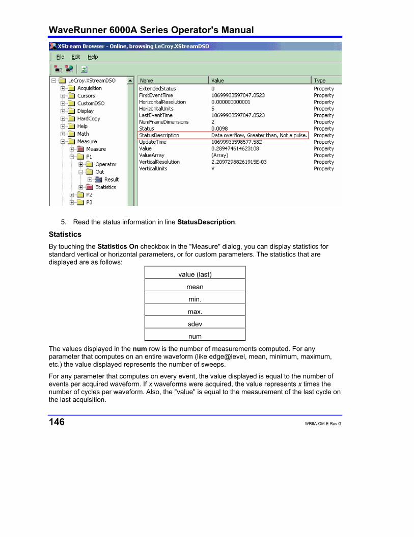
WaveRunner 6000A Series Operator's Manual
146 WR6A-OM-E Rev G
5. Read the status information in line StatusDescription.
Statistics By touching the Statistics On checkbox in the "Measure" dialog, you can display statistics for standard vertical or horizontal parameters, or for custom parameters. The statistics that are displayed are as follows:
value (last)
mean
min.
max.
sdev
num
The values displayed in the num row is the number of measurements computed. For any parameter that computes on an entire waveform (like edge@level, mean, minimum, maximum, etc.) the value displayed represents the number of sweeps.
For any parameter that computes on every event, the value displayed is equal to the number of events per acquired waveform. If x waveforms were acquired, the value represents x times the number of cycles per waveform. Also, the "value" is equal to the measurement of the last cycle on the last acquisition.

WR6A-OM-E Rev G 147
To Apply a Measure Mode 1. In the menu bar, touch Measure, then Measure Setup.
2. Choose a Measure Mode from the dialog. The parameters are displayed below the grid.
Measure Modes The selections for Measure Mode allow you to quickly apply parameters for standard vertical and standard horizontal setups, and custom setups. Standard Vertical Parameters
These are the default Standard Vertical Parameters:
Vertical
mean
sdev
max.
min.
ampl
pkpk
top
base
Standard Horizontal Parameters
These are the default Standard Horizontal Parameters:
Horizontal
freq
period
width
rise
fall
delay
duty
npoints
WaveRunner 6000A Series Operator's Manual
148 WR6A-OM-E Rev G
My Measure
You can choose to customize up to eight parameters by touching My Measure.
Parameter Math (XMATH or XMAP option required) The instrument gives you the ability to perform arithmetic operations (addition, subtraction, multiplication, division) on the results of two parameter measurements. Alternatively, you can apply math to a single parameter (for example, invert). By customizing parameters in this way, you can effectively extend the range of parameter measurements based on your particular needs. Logarithmic Parameters
The parameter math feature prevents multiplication and division of parameters that return logarithmic values. These parameters are as follows:
• auto-correlation signal-to-noise ratio (ACSN)
• narrow-band power (NBPW)
• media signal-to-noise ratio (MSNR)
• residual signal-to-noise ratio (RSNR)
• top-to-base ratio when the units are in dB (TBR) Excluded Parameters
Parameters that are already the result of parameter math operations are excluded. If they are included in a remote control setup command, an error message is generated and the setup canceled.
Excluded parameters are as follows:
• delta clock-to-data near (DC2D)
• delta clock-to-data next (DC2DPOS)
• delta clock-to-data previous (DC2DNEG)
• delta delay (DDLY)
• delta time at level (DTLEV)
• phase (PHASE)
• resolution (RES)
• mTnTmT shift (BEES)
• mTnTmT shift sigma (BEESS)
• mTnTmT shift sigma – list (BEESS)
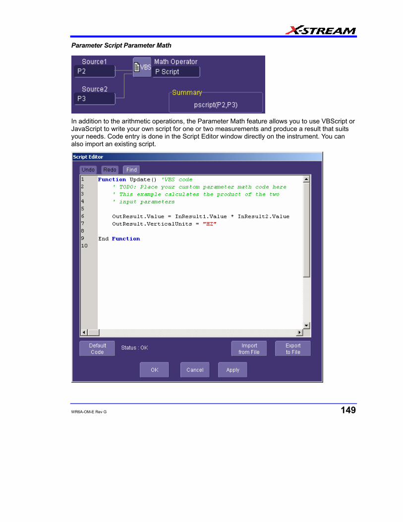
WR6A-OM-E Rev G 149
Parameter Script Parameter Math
In addition to the arithmetic operations, the Parameter Math feature allows you to use VBScript or JavaScript to write your own script for one or two measurements and produce a result that suits your needs. Code entry is done in the Script Editor window directly on the instrument. You can also import an existing script.
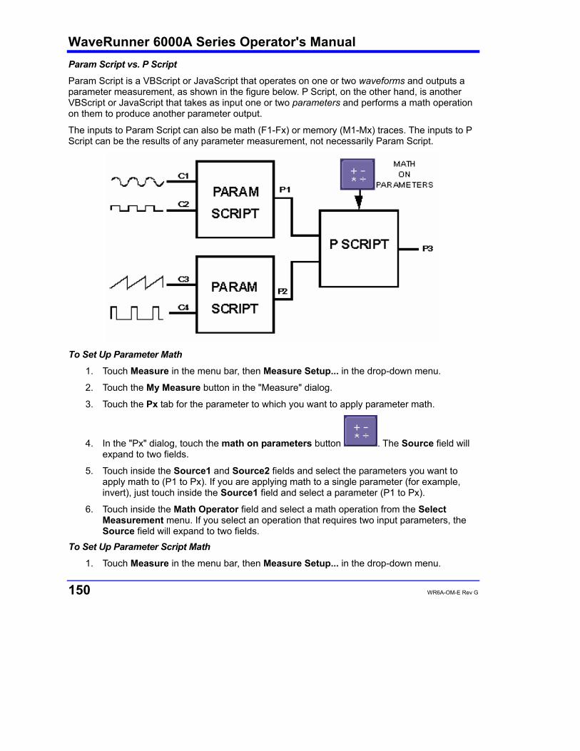
WaveRunner 6000A Series Operator's Manual
150 WR6A-OM-E Rev G
Param Script vs. P Script
Param Script is a VBScript or JavaScript that operates on one or two waveforms and outputs a parameter measurement, as shown in the figure below. P Script, on the other hand, is another VBScript or JavaScript that takes as input one or two parameters and performs a math operation on them to produce another parameter output.
The inputs to Param Script can also be math (F1-Fx) or memory (M1-Mx) traces. The inputs to P Script can be the results of any parameter measurement, not necessarily Param Script.
To Set Up Parameter Math
1. Touch Measure in the menu bar, then Measure Setup... in the drop-down menu.
2. Touch the My Measure button in the "Measure" dialog.
3. Touch the Px tab for the parameter to which you want to apply parameter math.
4. In the "Px" dialog, touch the math on parameters button . The Source field will expand to two fields.
5. Touch inside the Source1 and Source2 fields and select the parameters you want to apply math to (P1 to Px). If you are applying math to a single parameter (for example, invert), just touch inside the Source1 field and select a parameter (P1 to Px).
6. Touch inside the Math Operator field and select a math operation from the Select Measurement menu. If you select an operation that requires two input parameters, the Source field will expand to two fields.
To Set Up Parameter Script Math
1. Touch Measure in the menu bar, then Measure Setup... in the drop-down menu.
WR6A-OM-E Rev G 151
2. Touch the My Measure button in the "Measure" dialog.
3. Touch the Px tab for the parameter to which you want to apply parameter math.
4. In the "Px" dialog, touch the math on parameters button . The Source field will expand to two fields.
5. Touch inside the Source1 and Source2 fields and select the parameters you want to apply math to (P1 to Px). If you are applying math to a single parameter (for example, invert), just touch inside the Source1 field and select a parameter (P1 to Px).
6. Touch inside the Math Operator field and select P Script from the Select Measurement menu.
7. In the "Script Math" dialog, touch inside the Script Language field and select either VBScript or JScript from the pop-up menu.
8. Touch the Edit Code button; the Script Editor window opens. You can enter code in this window or call up an existing script from a file storage location. If you create your script in this window, you can then export it and save it to file.
Measure Gate Using Measure Gate, you can narrow the span of the waveform on which to perform parameter measurements, allowing you to focus on the area of greatest interest. You have the option of dragging the gate posts horizontally along the waveform, or specifying a position down to hundredths of a division. The default starting positions of the gate posts are 0 div and 10 div, which coincide with the left and right ends of the grid. The gate, therefore, initially encloses the entire waveform. Note: If you have Grid On Top enabled, you will not see the gate posts in their default position at each end of the grid. But
if you touch either end of the grid, a drag cursor will appear, indicating that you have control of the post and can now drag it.
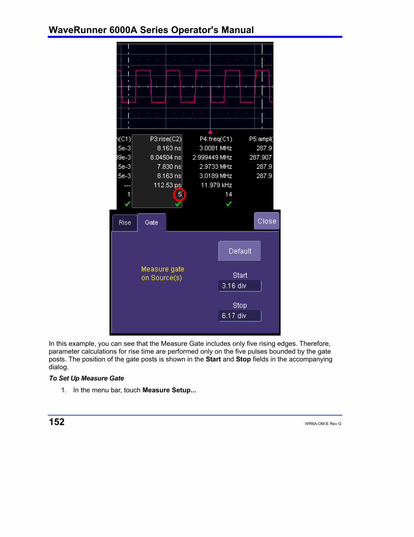
WaveRunner 6000A Series Operator's Manual
152 WR6A-OM-E Rev G
In this example, you can see that the Measure Gate includes only five rising edges. Therefore, parameter calculations for rise time are performed only on the five pulses bounded by the gate posts. The position of the gate posts is shown in the Start and Stop fields in the accompanying dialog. To Set Up Measure Gate
1. In the menu bar, touch Measure Setup...
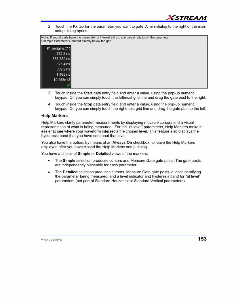
WR6A-OM-E Rev G 153
2. Touch the Px tab for the parameter you want to gate. A mini-dialog to the right of the main setup dialog opens.
Note: If you already have the parameter of interest set up, you can simply touch the parameter Example Parameter Readout directly below the grid.
3. Touch inside the Start data entry field and enter a value, using the pop-up numeric keypad. Or, you can simply touch the leftmost grid line and drag the gate post to the right.
4. Touch inside the Stop data entry field and enter a value, using the pop-up numeric keypad. Or, you can simply touch the rightmost grid line and drag the gate post to the left.
Help Markers Help Markers clarify parameter measurements by displaying movable cursors and a visual representation of what is being measured. For the "at level" parameters, Help Markers make it easier to see where your waveform intersects the chosen level. This feature also displays the hysteresis band that you have set about that level.
You also have the option, by means of an Always On checkbox, to leave the Help Markers displayed after you have closed the Help Markers setup dialog.
You have a choice of Simple or Detailed views of the markers:
• The Simple selection produces cursors and Measure Gate gate posts. The gate posts are independently placeable for each parameter.
• The Detailed selection produces cursors, Measure Gate gate posts, a label identifying the parameter being measured, and a level indicator and hysteresis band for "at level" parameters (not part of Standard Horizontal or Standard Vertical parameters).

WaveRunner 6000A Series Operator's Manual
154 WR6A-OM-E Rev G
Standard Horizontal Parameter Help Markers
Standard Vertical Parameter Help Markers
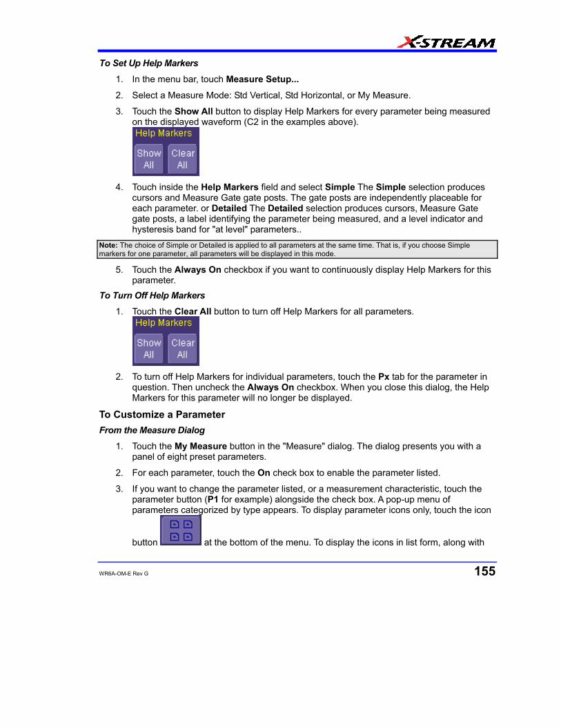
WR6A-OM-E Rev G 155
To Set Up Help Markers
1. In the menu bar, touch Measure Setup...
2. Select a Measure Mode: Std Vertical, Std Horizontal, or My Measure.
3. Touch the Show All button to display Help Markers for every parameter being measured on the displayed waveform (C2 in the examples above).
4. Touch inside the Help Markers field and select Simple The Simple selection produces
cursors and Measure Gate gate posts. The gate posts are independently placeable for each parameter. or Detailed The Detailed selection produces cursors, Measure Gate gate posts, a label identifying the parameter being measured, and a level indicator and hysteresis band for "at level" parameters..
Note: The choice of Simple or Detailed is applied to all parameters at the same time. That is, if you choose Simple markers for one parameter, all parameters will be displayed in this mode.
5. Touch the Always On checkbox if you want to continuously display Help Markers for this parameter.
To Turn Off Help Markers
1. Touch the Clear All button to turn off Help Markers for all parameters.
2. To turn off Help Markers for individual parameters, touch the Px tab for the parameter in
question. Then uncheck the Always On checkbox. When you close this dialog, the Help Markers for this parameter will no longer be displayed.
To Customize a Parameter From the Measure Dialog
1. Touch the My Measure button in the "Measure" dialog. The dialog presents you with a panel of eight preset parameters.
2. For each parameter, touch the On check box to enable the parameter listed.
3. If you want to change the parameter listed, or a measurement characteristic, touch the parameter button (P1 for example) alongside the check box. A pop-up menu of parameters categorized by type appears. To display parameter icons only, touch the icon
button at the bottom of the menu. To display the icons in list form, along with

WaveRunner 6000A Series Operator's Manual
156 WR6A-OM-E Rev G
an explanation of each parameter, touch the list button . Use the Up/Down buttons to scroll through the list of icons.
4. When you make a selection from the parameter icon menu, the setup dialogs for that parameter appear. You can then change the waveform source and other conditions of the parameter.
5. If you are setting up an "@level" parameter, make selections for Level type (percent or absolute), Slope (positive, negative, both), and Hysteresis level.
6. Touch the Gate tab, and set the position of the gate posts. From a Vertical Setup Dialog
1. In the "Cx Vertical Adjust" dialog, touch the Measure button .
2. Select a parameter from the pop-up menu. (The Actions for trace source defaults to the channel or trace whose dialog is open. If a parameter, it goes into the next "available" parameter, or the last one if all are used.)
3. Select another parameter or touch Close. From a Math Setup Dialog
1. In the "Fx" dialog, touch the Measure button .
2. Select a parameter from the pop-up menu. (The Actions for trace source defaults to the channel or trace whose dialog is open. If a parameter, it goes into the next "available" parameter, or the last one if all are used.)
3. Select another parameter or touch Close.
Parameter Calculations Parameters and How They Work
Determining Top and Base Lines
Proper determination of the top and base reference lines is fundamental for ensuring correct parameter calculations. The analysis begins by computing a histogram of the waveform data over the time interval spanned by the left and right time cursors. For example, the histogram of a waveform transitioning in two states will contain two peaks (see Figure 1). The analysis will attempt to identify the two clusters that contain the largest data density. Then the most probable state (centroids) associated with these two clusters will be computed to determine the top and base reference levels: the top line corresponds to the top and the base line to the bottom centroid.
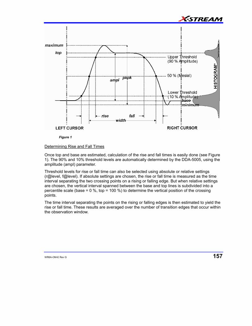
WR6A-OM-E Rev G 157
Figure 1
Determining Rise and Fall Times
Once top and base are estimated, calculation of the rise and fall times is easily done (see Figure 1). The 90% and 10% threshold levels are automatically determined by the DDA-5005, using the amplitude (ampl) parameter.
Threshold levels for rise or fall time can also be selected using absolute or relative settings (r@level, f@level). If absolute settings are chosen, the rise or fall time is measured as the time interval separating the two crossing points on a rising or falling edge. But when relative settings are chosen, the vertical interval spanned between the base and top lines is subdivided into a percentile scale (base = 0 %, top = 100 %) to determine the vertical position of the crossing points.
The time interval separating the points on the rising or falling edges is then estimated to yield the rise or fall time. These results are averaged over the number of transition edges that occur within the observation window.
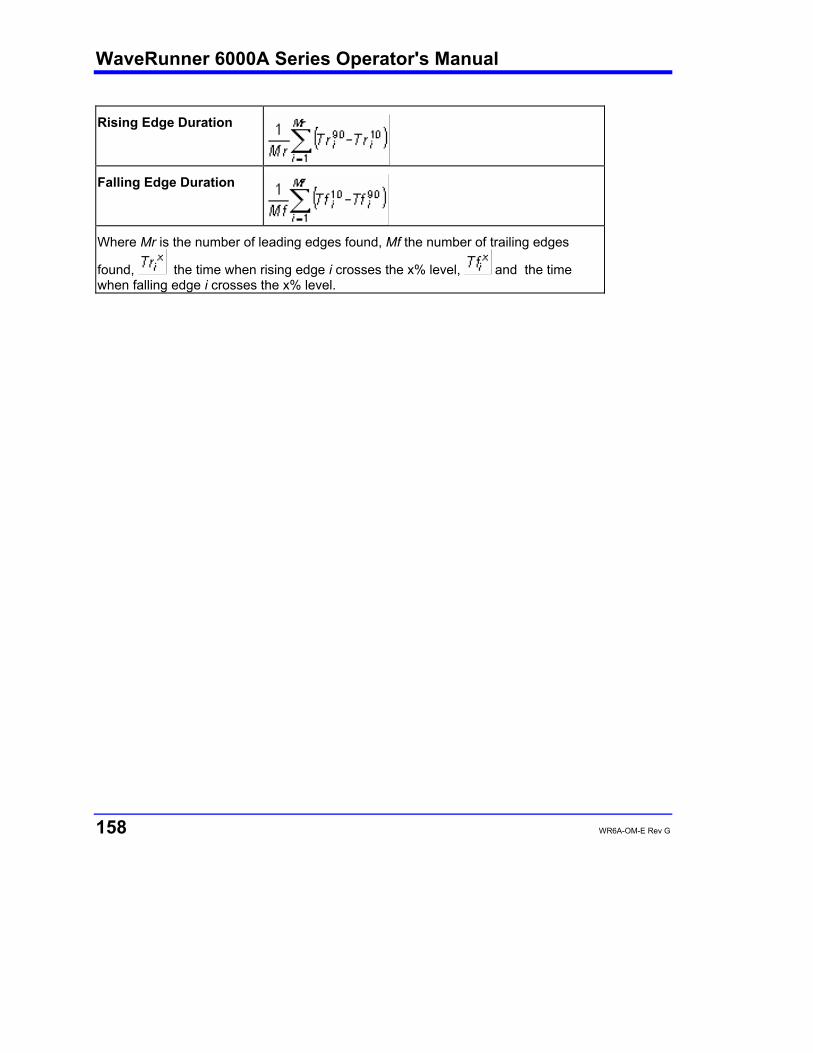
WaveRunner 6000A Series Operator's Manual
158 WR6A-OM-E Rev G
Rising Edge Duration
Falling Edge Duration
Where Mr is the number of leading edges found, Mf the number of trailing edges
found, the time when rising edge i crosses the x% level, and the time when falling edge i crosses the x% level.
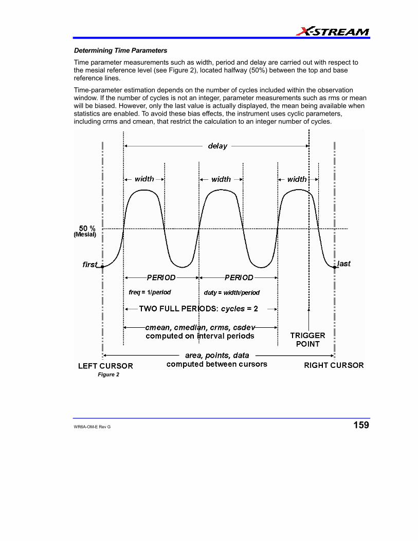
WR6A-OM-E Rev G 159
Determining Time Parameters
Time parameter measurements such as width, period and delay are carried out with respect to the mesial reference level (see Figure 2), located halfway (50%) between the top and base reference lines.
Time-parameter estimation depends on the number of cycles included within the observation window. If the number of cycles is not an integer, parameter measurements such as rms or mean will be biased. However, only the last value is actually displayed, the mean being available when statistics are enabled. To avoid these bias effects, the instrument uses cyclic parameters, including crms and cmean, that restrict the calculation to an integer number of cycles.
Figure 2
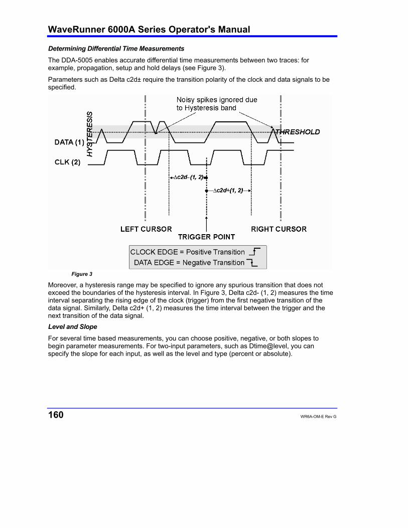
WaveRunner 6000A Series Operator's Manual
160 WR6A-OM-E Rev G
Determining Differential Time Measurements
The DDA-5005 enables accurate differential time measurements between two traces: for example, propagation, setup and hold delays (see Figure 3).
Parameters such as Delta c2d± require the transition polarity of the clock and data signals to be specified.
Figure 3
Moreover, a hysteresis range may be specified to ignore any spurious transition that does not exceed the boundaries of the hysteresis interval. In Figure 3, Delta c2d- (1, 2) measures the time interval separating the rising edge of the clock (trigger) from the first negative transition of the data signal. Similarly, Delta c2d+ (1, 2) measures the time interval between the trigger and the next transition of the data signal. Level and Slope
For several time based measurements, you can choose positive, negative, or both slopes to begin parameter measurements. For two-input parameters, such as Dtime@level, you can specify the slope for each input, as well as the level and type (percent or absolute).

WR6A-OM-E Rev G 161
List of Parameters The following table describes the instrument parameters. Availability of some parameters depends on the options installed. See the comments in the "Notes" column of the table.
Parameter Description Definition Notes
100BT Fall Fall time between 2 levels (upper-base, base-lower) of a 3-level signal (100BT)
Available with ENET option.
100BT Rise Rise time between 2 levels (Lower-base, base-upper) of a 3-level signal (100BT)
Available with ENET option.
100BT TIE Difference between the measured and ideal times at level between base and upper orlower levels of 100BT signal.
Available with ENET option.
100BT Tj Total jitter from a TIE at level between base and upper or lower levels of 100BTsignal.
Available with ENET option.
ACSN Auto-correlation Signal-to-Noise provides a signal-to-noise ratio for periodic waveforms.
Available with DDM2 option.
Standard in DDA-5005A.
AltNCycle Alternate N-Cycle Plot. Timing of the transitions in the data waveform is measured for each transition and plotted as a function of the number of unit intervals over which the timing is measured. The N-cycle plot displays the mean or standard deviation of the edge placement in the waveform relative to each other (data to data) or to a reference clock (clock to data).
Available with ASDA option.
Amplitude Measures the difference between upper and lower levels in two-level signals. Differs from pkpk in that noise, overshoot, undershoot, and ringing do not affect the measurement.
top - base On signals not having two major levels (such as triangle or saw-tooth waves), returns same value as pkpk.
Standard parameter.
Ampl asym Amplitude asymmetry between taa+ and taa-
1 |(taa+ - taa-)|/(taa+ - taa-) Hysteresis argument used to discriminate levels from noise in data.
WaveRunner 6000A Series Operator's Manual
162 WR6A-OM-E Rev G
Available with DDM2 option.
Standard in DDA-5005A.
Area Integral of data: Computes area of waveform between cursors relative to zero level. Values greater than zero contribute positively to the area; values less than zero negatively.
Sum from first to last of data multiplied by horizontal time between points
Standard parameter..
Avg Power Average power of the waveform Available with SDA and SDM options.
Standard in SDA100G scopes.
Base Lower of two most probable states (higher is top). Measures lower level in two-level signals. Differs from min in that noise, overshoot, undershoot, and ringing do not affect measurement.
Value of most probable lower state
On signals not having two major levels (triangle or saw-tooth waves, for example), returns same value as min.
Standard parameter.
Bit Rate One over duration of one UI measured on an eye
Available with SDA option.
Standard in SDA, SDA100G, and WaveExpert scopes.
CMACp PCI Express V TX-CM-ACp and V RX-CM-Acp
Available with PCIE option.
Cycles Determines number of cycles of a periodic waveform lying between cursors. First cycle begins at first transition after the left cursor. Transition may be positive- or negative-going.
Number of cycles of periodic waveform
Standard parameter.
cyclic
Mean
Cyclic mean: Computes the average of waveform data. Contrary to mean, computes average over an integral number of cycles, eliminating bias caused by fractional intervals.
Average of data values of an integral number of periods
Choose this parameter by selecting Mean from the parameter table, then touching the Cyclic checkbox.
Standard parameter.

WR6A-OM-E Rev G 163
cyclic
Median
Cyclic median: Computes average of base and top values over an integral number of cycles, contrary to median, eliminating bias caused by fractional intervals.
Data value for which 50% of values are above and 50% below
Choose this parameter by selecting Median from the parameter table, then touching the Cyclic checkbox.
Standard parameter.
cyclic
RMS
Cyclic root mean square: Computes square root of sum of squares of data values divided by number of points. Contrary to rms, calculation is performed over an integral number of cycles, eliminating bias caused by fractional intervals.
Where: vi denotes measured sample values, and N = number of data points within the periods found.
Choose this parameter by selecting RMS from the parameter table, then touching the Cyclic checkbox.
Standard parameter.
cyclic
Std dev
Cyclic standard deviation: Standard deviation of data values from mean value over integral number of periods. Contrary to sdev, calculation is performed over an integral number of cycles, eliminating bias caused by fractional intervals.
Where: vi denotes measured sample values, and N = number of data points within the periods found.
Choose this parameter by selecting Std dev from the parameter table, then touching the Cyclic checkbox.
Standard parameter.
DCD Amount of jitter due to duty cycle distortion
Available with SDA and ENET options.
Standard in SDA and WaveExpert scopes.
DDj Amount of data dependent jitter in a signal
Available with SDA option.
Delay Time from trigger to transition: Measures time between trigger and first 50% crossing after left cursor. Can measure propagation delay between two signals by triggering on one and determining delay of other.
Time between trigger and first 50% crossing after left cursor
Standard parameter.

WaveRunner 6000A Series Operator's Manual
164 WR6A-OM-E Rev G
Delta delay delay: Computes time between 50% level of two sources.
Time between midpoint transition of two sources
Standard parameter.
Dj Effective Amount of deterministic jitter (estimated) in a signal
Available with SDA option.
DOV Differential Output Voltage of a 100Base-T signal
Available with ENET option.
Dperiod@level Adjacent cycle deviation (cycle-to-cycle jitter) of each cycle in a waveform
Reference levels and edge-transition polarity can be selected. Hysteresis argument used to discriminate levels from noise in data.
Available with JTA2 and XMAP options.
Standard in SDA100G scopes.
Droop FG 1000Base-T test mode 1 droop from F to G
Available with ENET option.
Droop HJ 1000Base-T test mode 1 droop from H to J
Available with ENET option.
Dtime@level t at level: Computes transition between selected levels or sources.
Time between transition levels of two sources, or from trigger to transition level of a single source
This measurement gives the time of the source 2 edge minus the time of the source 1 edge.
Reference levels and edge-transition polarity can be selected. Hysteresis argument used to discriminate levels from noise in data.
Standard parameter.
Dtrig Time Time from last trigger to this trigger Standard in WaveRunner 6000A, WavePro 7000A, WaveMaster, and sampling scopes.
Duration For single sweep waveforms, dur is 0; for sequence waveforms: time from first to last segment's trigger; for single segments of sequence waveforms: time from previous segment's to current segment's trigger; for waveforms produced by a history function: time from first to last accumulated waveform's trigger.
Time from first to last acquisition: for average, histogram or sequence waveforms
Standard parameter.

WR6A-OM-E Rev G 165
Duty@level Percent of period for which data are above or below a specified level.
Reference levels and edge-transition polarity can be selected. Hysteresis argument used to discriminate levels from noise in data.
Available with JTA2 and XMAP options.
Duty cycle Duty cycle: Width as percentage of period.
width/period Standard parameter.
Dwidth@level Difference of adjacent width above or below a specified level.
Reference levels and edge-transition polarity can be selected. Hysteresis argument used to discriminate levels from noise in data.
Available with JTA2 and XMAP options.
Standard in SDA100G scopes.
Edge@level Number of edges in waveform. Reference levels and edge-transition polarity can be selected. Hysteresis argument used to discriminate levels from noise in data.
Available with JTA2, USB2, SDA, and XMAP options.
Standard in SDA100G and WavePro 7000A scopes.
Ext Ratio Ratio of the power levels of an eye diagram
Available with SDA and SDM options.
Standard in SDA, SDA100G, and WaveExpert scopes.
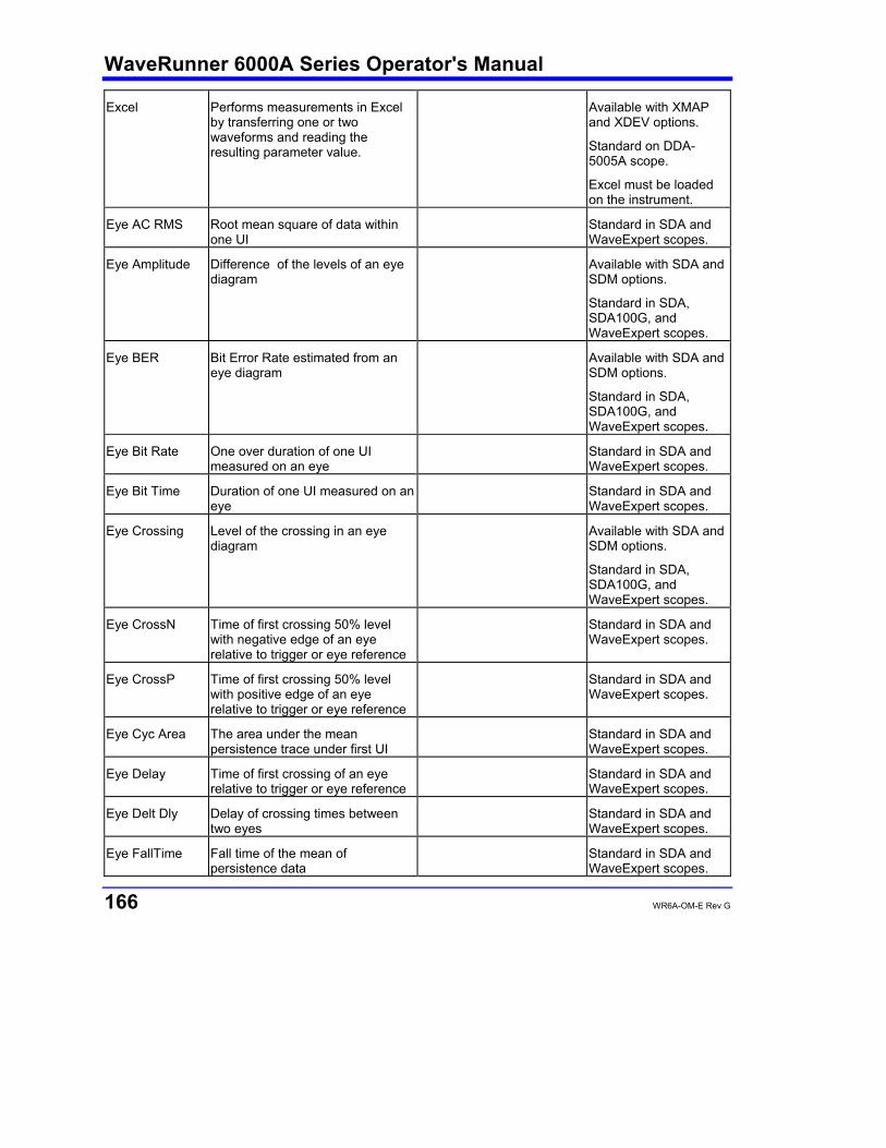
WaveRunner 6000A Series Operator's Manual
166 WR6A-OM-E Rev G
Excel Performs measurements in Excel by transferring one or two waveforms and reading the resulting parameter value.
Available with XMAP and XDEV options.
Standard on DDA-5005A scope.
Excel must be loaded on the instrument.
Eye AC RMS Root mean square of data within one UI
Standard in SDA and WaveExpert scopes.
Eye Amplitude Difference of the levels of an eye diagram
Available with SDA and SDM options.
Standard in SDA, SDA100G, and WaveExpert scopes.
Eye BER Bit Error Rate estimated from an eye diagram
Available with SDA and SDM options.
Standard in SDA, SDA100G, and WaveExpert scopes.
Eye Bit Rate One over duration of one UI measured on an eye
Standard in SDA and WaveExpert scopes.
Eye Bit Time Duration of one UI measured on an eye
Standard in SDA and WaveExpert scopes.
Eye Crossing Level of the crossing in an eye diagram
Available with SDA and SDM options.
Standard in SDA, SDA100G, and WaveExpert scopes.
Eye CrossN Time of first crossing 50% level with negative edge of an eye relative to trigger or eye reference
Standard in SDA and WaveExpert scopes.
Eye CrossP Time of first crossing 50% level with positive edge of an eye relative to trigger or eye reference
Standard in SDA and WaveExpert scopes.
Eye Cyc Area The area under the mean persistence trace under first UI
Standard in SDA and WaveExpert scopes.
Eye Delay Time of first crossing of an eye relative to trigger or eye reference
Standard in SDA and WaveExpert scopes.
Eye Delt Dly Delay of crossing times between two eyes
Standard in SDA and WaveExpert scopes.
Eye FallTime Fall time of the mean of persistence data
Standard in SDA and WaveExpert scopes.
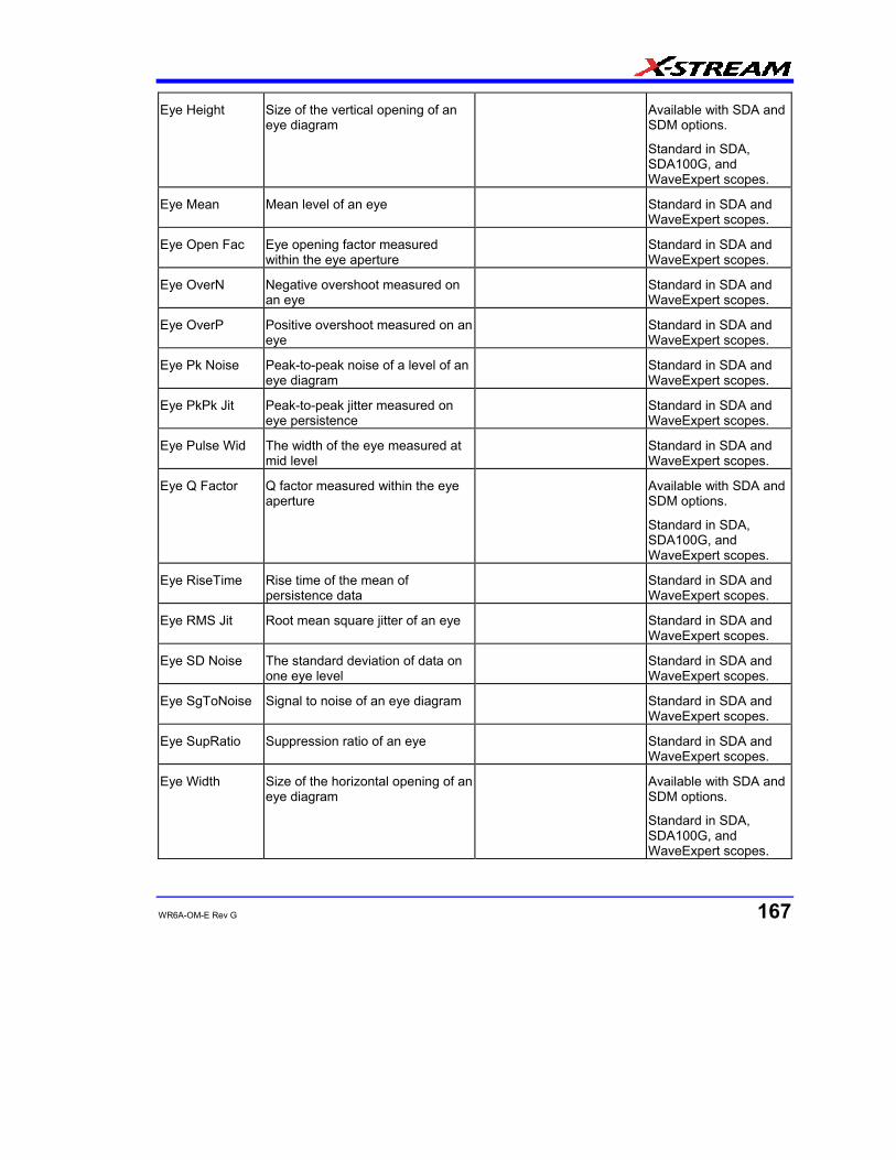
WR6A-OM-E Rev G 167
Eye Height Size of the vertical opening of an eye diagram
Available with SDA and SDM options.
Standard in SDA, SDA100G, and WaveExpert scopes.
Eye Mean Mean level of an eye Standard in SDA and WaveExpert scopes.
Eye Open Fac Eye opening factor measured within the eye aperture
Standard in SDA and WaveExpert scopes.
Eye OverN Negative overshoot measured on an eye
Standard in SDA and WaveExpert scopes.
Eye OverP Positive overshoot measured on an eye
Standard in SDA and WaveExpert scopes.
Eye Pk Noise Peak-to-peak noise of a level of an eye diagram
Standard in SDA and WaveExpert scopes.
Eye PkPk Jit Peak-to-peak jitter measured on eye persistence
Standard in SDA and WaveExpert scopes.
Eye Pulse Wid The width of the eye measured at mid level
Standard in SDA and WaveExpert scopes.
Eye Q Factor Q factor measured within the eye aperture
Available with SDA and SDM options.
Standard in SDA, SDA100G, and WaveExpert scopes.
Eye RiseTime Rise time of the mean of persistence data
Standard in SDA and WaveExpert scopes.
Eye RMS Jit Root mean square jitter of an eye Standard in SDA and WaveExpert scopes.
Eye SD Noise The standard deviation of data on one eye level
Standard in SDA and WaveExpert scopes.
Eye SgToNoise Signal to noise of an eye diagram Standard in SDA and WaveExpert scopes.
Eye SupRatio Suppression ratio of an eye Standard in SDA and WaveExpert scopes.
Eye Width Size of the horizontal opening of an eye diagram
Available with SDA and SDM options.
Standard in SDA, SDA100G, and WaveExpert scopes.
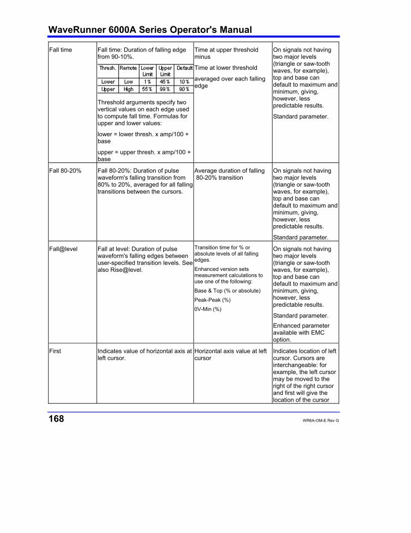
WaveRunner 6000A Series Operator's Manual
168 WR6A-OM-E Rev G
Fall time Fall time: Duration of falling edge from 90-10%.
Threshold arguments specify two vertical values on each edge used to compute fall time. Formulas for upper and lower values:
lower = lower thresh. x amp/100 + base
upper = upper thresh. x amp/100 + base
Time at upper threshold minus
Time at lower threshold
averaged over each falling edge
On signals not having two major levels (triangle or saw-tooth waves, for example), top and base can default to maximum and minimum, giving, however, less predictable results.
Standard parameter.
Fall 80-20% Fall 80-20%: Duration of pulse waveform's falling transition from 80% to 20%, averaged for all falling transitions between the cursors.
Average duration of falling 80-20% transition
On signals not having two major levels (triangle or saw-tooth waves, for example), top and base can default to maximum and minimum, giving, however, less predictable results.
Standard parameter.
Fall@level Fall at level: Duration of pulse waveform's falling edges between user-specified transition levels. See also Rise@level.
Transition time for % or absolute levels of all falling edges.
Enhanced version sets measurement calculations to use one of the following:
Base & Top (% or absolute)
Peak-Peak (%)
0V-Min (%)
On signals not having two major levels (triangle or saw-tooth waves, for example), top and base can default to maximum and minimum, giving, however, less predictable results.
Standard parameter. Enhanced parameter available with EMC option.
First Indicates value of horizontal axis at left cursor.
Horizontal axis value at left cursor
Indicates location of left cursor. Cursors are interchangeable: for example, the left cursor may be moved to the right of the right cursor and first will give the location of the cursor
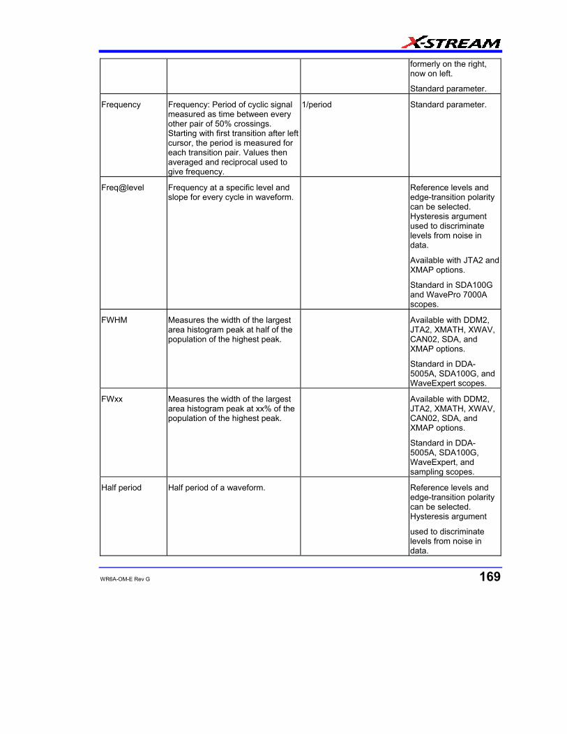
WR6A-OM-E Rev G 169
formerly on the right, now on left.
Standard parameter.
Frequency Frequency: Period of cyclic signal measured as time between every other pair of 50% crossings. Starting with first transition after left cursor, the period is measured for each transition pair. Values then averaged and reciprocal used to give frequency.
1/period Standard parameter.
Freq@level Frequency at a specific level and slope for every cycle in waveform.
Reference levels and edge-transition polarity can be selected. Hysteresis argument used to discriminate levels from noise in data.
Available with JTA2 and XMAP options.
Standard in SDA100G and WavePro 7000A scopes.
FWHM Measures the width of the largest area histogram peak at half of the population of the highest peak.
Available with DDM2, JTA2, XMATH, XWAV, CAN02, SDA, and XMAP options.
Standard in DDA-5005A, SDA100G, and WaveExpert scopes.
FWxx Measures the width of the largest area histogram peak at xx% of the population of the highest peak.
Available with DDM2, JTA2, XMATH, XWAV, CAN02, SDA, and XMAP options.
Standard in DDA-5005A, SDA100G, WaveExpert, and sampling scopes.
Half period Half period of a waveform. Reference levels and edge-transition polarity can be selected. Hysteresis argument
used to discriminate levels from noise in data.
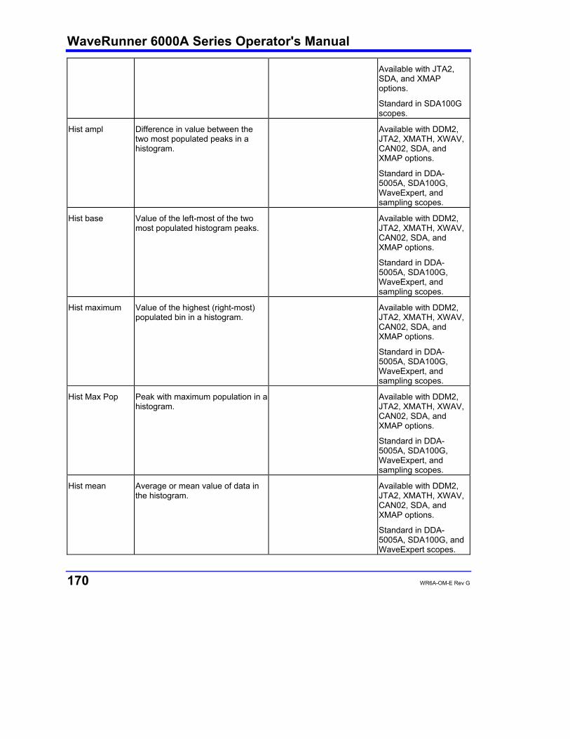
WaveRunner 6000A Series Operator's Manual
170 WR6A-OM-E Rev G
Available with JTA2, SDA, and XMAP options.
Standard in SDA100G scopes.
Hist ampl Difference in value between the two most populated peaks in a histogram.
Available with DDM2, JTA2, XMATH, XWAV, CAN02, SDA, and XMAP options.
Standard in DDA-5005A, SDA100G, WaveExpert, and sampling scopes.
Hist base Value of the left-most of the two most populated histogram peaks.
Available with DDM2, JTA2, XMATH, XWAV, CAN02, SDA, and XMAP options.
Standard in DDA-5005A, SDA100G, WaveExpert, and sampling scopes.
Hist maximum Value of the highest (right-most) populated bin in a histogram.
Available with DDM2, JTA2, XMATH, XWAV, CAN02, SDA, and XMAP options.
Standard in DDA-5005A, SDA100G, WaveExpert, and sampling scopes.
Hist Max Pop Peak with maximum population in a histogram.
Available with DDM2, JTA2, XMATH, XWAV, CAN02, SDA, and XMAP options.
Standard in DDA-5005A, SDA100G, WaveExpert, and sampling scopes.
Hist mean Average or mean value of data in the histogram.
Available with DDM2, JTA2, XMATH, XWAV, CAN02, SDA, and XMAP options.
Standard in DDA-5005A, SDA100G, and WaveExpert scopes.

WR6A-OM-E Rev G 171
Hist median Value of the "X" axis of a histogram that divides the population into two equal halves.
Available with DDM2, JTA2, XMATH, XWAV, CAN02, SDA, and XMAP options.
Standard in DDA-5005A, SDA100G, WaveExpert, and sampling scopes.
Hist minimum Value of the lowest (left-most) populated bin in a histogram.
Available with DDM2, JTA2, XMATH, XWAV, CAN02, SDA, and XMAP options.
Standard in DDA-5005A, SDA100G, and WaveExpert scopes.
Hist Mode Position of the highest histogram peak.
Available with DDM2, JTA2, XMATH, XWAV, CAN02, SDA, and XMAP options.
Standard in DDA-5005A, SDA100G, WaveExpert, and sampling scopes.
Hist Pop@X Population at bin for specified horizontal coordinate. You can place the cursor at any bin and use either Absolute, Reference, or Difference cursor shape.
Available with DDM2, JTA2, SDM, XMATH, XWAV, CAN02, SDA, and XMAP options.
Standard in DDA-5005A, SDA100G, and sampling scopes.
Hist Range Calculates range (max - min) of a histogram.
Available with DDM2, JTA2, ENET, XMATH, XWAV, CAN02, SDA, and XMAP options.
Standard in DDA-5005A, SDA100G, WaveExpert, and sampling scopes.
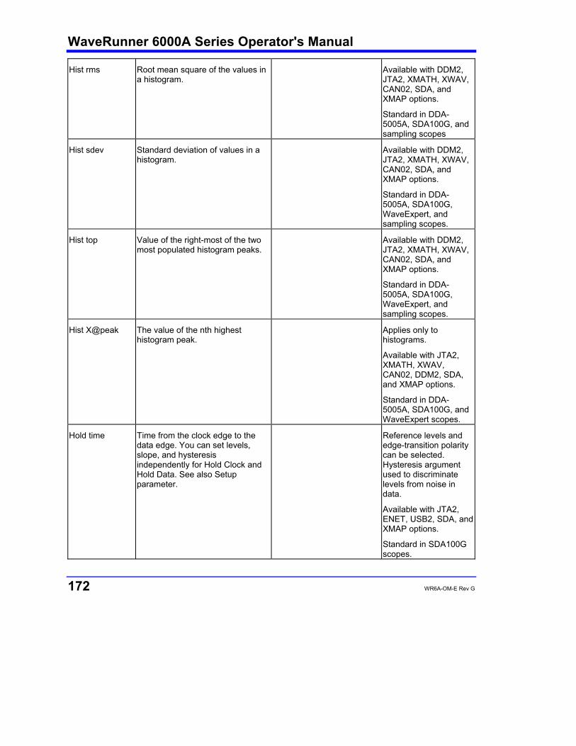
WaveRunner 6000A Series Operator's Manual
172 WR6A-OM-E Rev G
Hist rms Root mean square of the values in a histogram.
Available with DDM2, JTA2, XMATH, XWAV, CAN02, SDA, and XMAP options.
Standard in DDA-5005A, SDA100G, and sampling scopes
Hist sdev Standard deviation of values in a histogram.
Available with DDM2, JTA2, XMATH, XWAV, CAN02, SDA, and XMAP options.
Standard in DDA-5005A, SDA100G, WaveExpert, and sampling scopes.
Hist top Value of the right-most of the two most populated histogram peaks.
Available with DDM2, JTA2, XMATH, XWAV, CAN02, SDA, and XMAP options.
Standard in DDA-5005A, SDA100G, WaveExpert, and sampling scopes.
Hist X@peak The value of the nth highest histogram peak.
Applies only to histograms.
Available with JTA2, XMATH, XWAV, CAN02, DDM2, SDA, and XMAP options.
Standard in DDA-5005A, SDA100G, and WaveExpert scopes.
Hold time Time from the clock edge to the data edge. You can set levels, slope, and hysteresis independently for Hold Clock and Hold Data. See also Setup parameter.
Reference levels and edge-transition polarity can be selected. Hysteresis argument used to discriminate levels from noise in data.
Available with JTA2, ENET, USB2, SDA, and XMAP options.
Standard in SDA100G scopes.
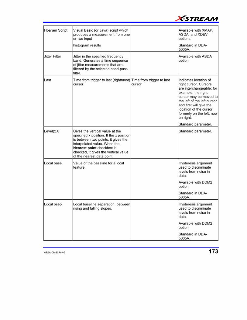
WR6A-OM-E Rev G 173
Hparam Script Visual Basic (or Java) script which produces a measurement from one or two input
histogram results
Available with XMAP, ASDA, and XDEV options.
Standard in DDA-5005A.
Jitter Filter Jitter in the specified frequency band. Generates a time sequence of jitter measurements that are filtered by the selected band-pass filter.
Available with ASDA option.
Last Time from trigger to last (rightmost) cursor.
Time from trigger to last cursor
Indicates location of right cursor. Cursors are interchangeable: for example, the right cursor may be moved to the left of the left cursor and first will give the location of the cursor formerly on the left, now on right.
Standard parameter.
Level@X Gives the vertical value at the specified x position. If the x position is between two points, it gives the interpolated value. When the Nearest point checkbox is checked, it gives the vertical value of the nearest data point.
Standard parameter.
Local base Value of the baseline for a local feature.
Hysteresis argument used to discriminate levels from noise in data.
Available with DDM2 option.
Standard in DDA-5005A.
Local bsep Local baseline separation, between rising and falling slopes.
Hysteresis argument used to discriminate levels from noise in data.
Available with DDM2 option.
Standard in DDA-5005A.

WaveRunner 6000A Series Operator's Manual
174 WR6A-OM-E Rev G
Local max Maximum value of a local feature. Hysteresis argument used to discriminate levels from noise in data.
Available with DDM2 option.
Standard in DDA-5005A.
Local min Minimum value of a local feature. Hysteresis argument used to discriminate levels from noise in data.
Available with DDM2 option.
Standard in DDA-5005A.
Local number Number of local features (peak/trough pairs).
Hysteresis argument used to discriminate levels from noise in data.
Available with DDM2 option.
Standard in DDA-5005A.
Local pkpk Vertical difference between the peak and trough of a local feature (lmax lmin).
Hysteresis argument used to discriminate levels from noise in data.
Available with DDM2 option.
Standard in DDA-5005A.
Local tbe Time between events (between local peak and next trough or local trough and next peak).
Hysteresis argument used to discriminate levels from noise in data.
Available with DDM2 option.
Standard in DDA-5005A.
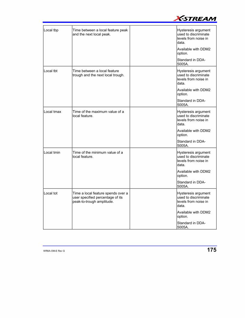
WR6A-OM-E Rev G 175
Local tbp Time between a local feature peak and the next local peak.
Hysteresis argument used to discriminate levels from noise in data.
Available with DDM2 option.
Standard in DDA-5005A.
Local tbt Time between a local feature trough and the next local trough.
Hysteresis argument used to discriminate levels from noise in data.
Available with DDM2 option.
Standard in DDA-5005A.
Local tmax Time of the maximum value of a local feature.
Hysteresis argument used to discriminate levels from noise in data.
Available with DDM2 option.
Standard in DDA-5005A.
Local tmin Time of the minimum value of a local feature.
Hysteresis argument used to discriminate levels from noise in data.
Available with DDM2 option.
Standard in DDA-5005A.
Local tot Time a local feature spends over a user specified percentage of its peak-to-trough amplitude.
Hysteresis argument used to discriminate levels from noise in data.
Available with DDM2 option.
Standard in DDA-5005A.

WaveRunner 6000A Series Operator's Manual
176 WR6A-OM-E Rev G
Local tpt Time between local feature peak and trough.
Hysteresis argument used to discriminate levels from noise in data.
Available with DDM2 option.
Standard in DDA-5005A.
Local ttp Time between local feature trough and the next local peak.
Hysteresis argument used to discriminate levels from noise in data.
Available with DDM2 option.
Standard in DDA-5005A.
Local tut Time a local feature spends under a user specified percentage of its peak-to-trough amplitude.
Hysteresis argument used to discriminate levels from noise in data.
Available with DDM2 option.
Standard in DDA-5005A.
Mathcad Produces a parameter using a user-specified Mathcad function.
Available with XMAP and XDEV option.
Standard in DDA-5005A.
Mathcad 2001i or later must be loaded on the instrument.
MATLAB Produces a parameter using a user-specified MATLAB function.
Available with XMAP and XDEV option.
Standard in DDA-5005A, WaveRunner 6000A, WaveMaster, WavePro 7000A, and sampling scopes
MATLAB must be loaded on the instrument.
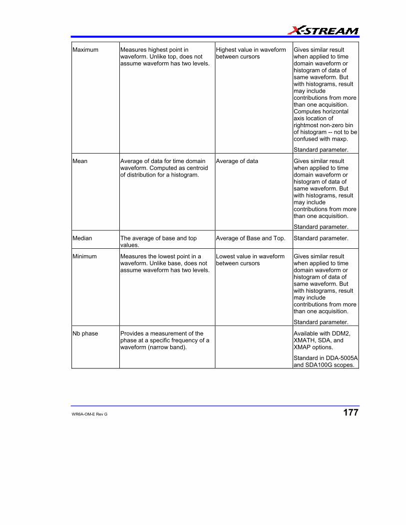
WR6A-OM-E Rev G 177
Maximum Measures highest point in waveform. Unlike top, does not assume waveform has two levels.
Highest value in waveform between cursors
Gives similar result when applied to time domain waveform or histogram of data of same waveform. But with histograms, result may include contributions from more than one acquisition. Computes horizontal axis location of rightmost non-zero bin of histogram -- not to be confused with maxp.
Standard parameter.
Mean Average of data for time domain waveform. Computed as centroid of distribution for a histogram.
Average of data Gives similar result when applied to time domain waveform or histogram of data of same waveform. But with histograms, result may include contributions from more than one acquisition.
Standard parameter.
Median The average of base and top values.
Average of Base and Top. Standard parameter.
Minimum Measures the lowest point in a waveform. Unlike base, does not assume waveform has two levels.
Lowest value in waveform between cursors
Gives similar result when applied to time domain waveform or histogram of data of same waveform. But with histograms, result may include contributions from more than one acquisition.
Standard parameter.
Nb phase Provides a measurement of the phase at a specific frequency of a waveform (narrow band).
Available with DDM2, XMATH, SDA, and XMAP options.
Standard in DDA-5005A and SDA100G scopes.
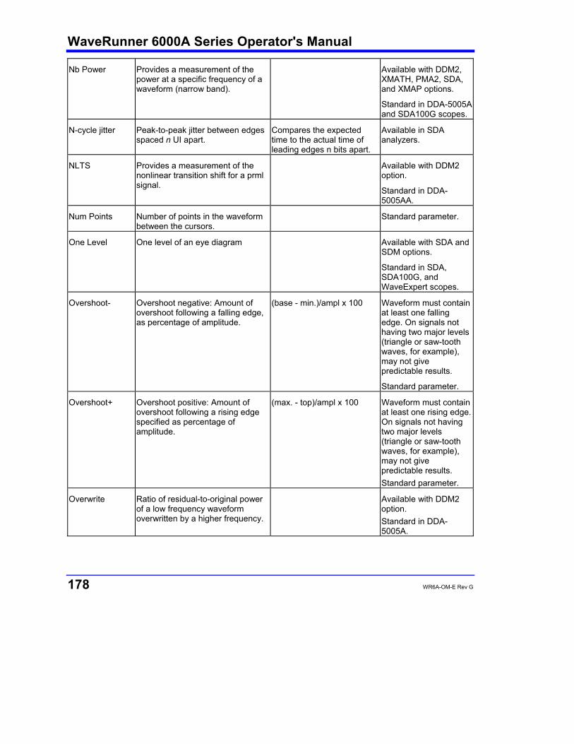
WaveRunner 6000A Series Operator's Manual
178 WR6A-OM-E Rev G
Nb Power Provides a measurement of the power at a specific frequency of a waveform (narrow band).
Available with DDM2, XMATH, PMA2, SDA, and XMAP options.
Standard in DDA-5005A and SDA100G scopes.
N-cycle jitter Peak-to-peak jitter between edges spaced n UI apart.
Compares the expected time to the actual time of leading edges n bits apart.
Available in SDA analyzers.
NLTS Provides a measurement of the nonlinear transition shift for a prml signal.
Available with DDM2 option.
Standard in DDA-5005AA.
Num Points Number of points in the waveform between the cursors.
Standard parameter.
One Level One level of an eye diagram Available with SDA and SDM options.
Standard in SDA, SDA100G, and WaveExpert scopes.
Overshoot- Overshoot negative: Amount of overshoot following a falling edge, as percentage of amplitude.
(base - min.)/ampl x 100 Waveform must contain at least one falling edge. On signals not having two major levels (triangle or saw-tooth waves, for example), may not give predictable results.
Standard parameter.
Overshoot+ Overshoot positive: Amount of overshoot following a rising edge specified as percentage of amplitude.
(max. - top)/ampl x 100 Waveform must contain at least one rising edge. On signals not having two major levels (triangle or saw-tooth waves, for example), may not give predictable results. Standard parameter.
Overwrite Ratio of residual-to-original power of a low frequency waveform overwritten by a higher frequency.
Available with DDM2 option. Standard in DDA-5005A.
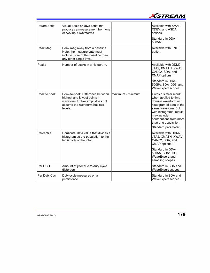
WR6A-OM-E Rev G 179
Param Script Visual Basic or Java script that produces a measurement from one or two input waveforms.
Available with XMAP, XDEV, and ASDA options.
Standard in DDA-5005A.
Peak Mag Peak mag away from a baseline. Note: the measure gate must include more of the baseline than any other single level.
Available with ENET option.
Peaks Number of peaks in a histogram. Available with DDM2, JTA2, XMATH, XWAV, CAN02, SDA, and XMAP options.
Standard in DDA-5005A, SDA100G, and WaveExpert scopes.
Peak to peak Peak-to-peak: Difference between highest and lowest points in waveform. Unlike ampl, does not assume the waveform has two levels.
maximum - minimum Gives a similar result when applied to time domain waveform or histogram of data of the same waveform. But with histograms, result may include contributions from more than one acquisition. Standard parameter.
Percentile Horizontal data value that divides a histogram so the population to the left is xx% of the total.
Available with DDM2, JTA2, XMATH, XWAV, CAN02, SDA, and XMAP options.
Standard in DDA-5005A, SDA100G, WaveExpert, and sampling scopes.
Per DCD Amount of jitter due to duty cycle distortion
Standard in SDA and WaveExpert scopes.
Per Duty Cyc Duty cycle measured on a persistence
Standard in SDA and WaveExpert scopes.

WaveRunner 6000A Series Operator's Manual
180 WR6A-OM-E Rev G
Period Period of a cyclic signal measured as time between every other pair of 50% crossings. Starting with first transition after left cursor, period is measured for each transition pair, with values averaged to give final result. Where: Mr is the number of
leading edges found, Mf the number of trailing edges
found, the time when rising edge i crosses the x%
level, and the time when falling edge i crosses the x% level.
Standard parameter.
Period@level Period at a specified level and slope for every cycle in waveform.
Reference levels and edge-transition polarity can be selected. Hysteresis argument used to discriminate levels from noise in data.
Available with JTA2, AORM, ENET, SDA, and XMAP options.
Standard in DDA-5005A, SDA100G, and WavePro 7000A scopes.
Per Pulse Sym Symmetry of RZ pulse around eye aperture center
Standard in SDA and WaveExpert scopes.
Persist Area Area under mean persistence trace Standard in SDA and WaveExpert scopes.
Persist Max Highest vertical value of input persistence
Standard in SDA and WaveExpert scopes.
Persist Mean Average of persistence data Standard in SDA and WaveExpert scopes.
Persist Mid Mid level between Maximum and Minimum data
Standard in SDA and WaveExpert scopes.
Persist Min Lowest vertical value of input persistence
Standard in SDA and WaveExpert scopes.
Persist PkPk Difference between maximum and minimum data values
Standard in SDA and WaveExpert scopes.
Persist RMS Root mean square of persistence data
Standard in SDA and WaveExpert scopes.
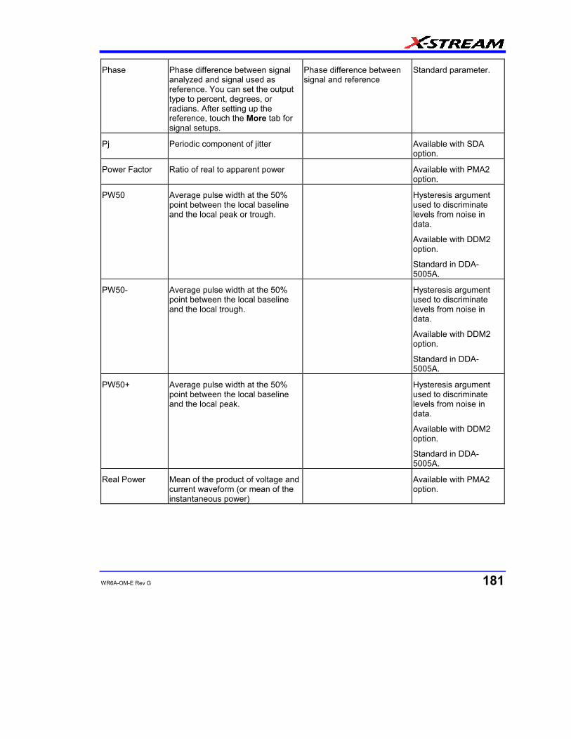
WR6A-OM-E Rev G 181
Phase Phase difference between signal analyzed and signal used as reference. You can set the output type to percent, degrees, or radians. After setting up the reference, touch the More tab for signal setups.
Phase difference between signal and reference
Standard parameter.
Pj Periodic component of jitter Available with SDA option.
Power Factor Ratio of real to apparent power Available with PMA2 option.
PW50 Average pulse width at the 50% point between the local baseline and the local peak or trough.
Hysteresis argument used to discriminate levels from noise in data.
Available with DDM2 option.
Standard in DDA-5005A.
PW50- Average pulse width at the 50% point between the local baseline and the local trough.
Hysteresis argument used to discriminate levels from noise in data.
Available with DDM2 option.
Standard in DDA-5005A.
PW50+ Average pulse width at the 50% point between the local baseline and the local peak.
Hysteresis argument used to discriminate levels from noise in data.
Available with DDM2 option.
Standard in DDA-5005A.
Real Power Mean of the product of voltage and current waveform (or mean of the instantaneous power)
Available with PMA2 option.

WaveRunner 6000A Series Operator's Manual
182 WR6A-OM-E Rev G
Resolution Ratio of taa for a high and low frequency waveform
taa (HF)/mean taa (LF)*100 Hysteresis argument used to discriminate levels from noise in data.
Available in DDM2.
Standard in DDA-5005A.
Ring Ringback (high or low) Available with SDA parameter.
Rj Effective Amount of random jitter (estimated) in a signal
Available with SDA parameter.
Rise Rise time: Duration of rising edge from 10-90%.
Threshold arguments specify two vertical values on each edge used to compute rise time.
Formulas for upper and lower values:
lower = lower thresh. x amp/100 + base
upper = upper thresh. x amp/100 + base
Time at lower threshold minus
Time at upper threshold
averaged over each rising edge
On signals not having two major levels (triangle or saw-tooth waves, for example), top and base can default to maximum and minimum, giving, however, less predictable results.
Standard parameter.
Rise 20-80% Rise 20% to 80%: Duration of pulse waveform's rising transition from 20% to 80%, averaged for all rising transitions between the cursors.
Average duration of rising 20-80% transition
On signals not having two major levels (triangle or saw-tooth waves, for example), top and base can default to maximum and minimum, giving, however, less predictable results.
Standard parameter.
Rise@level Rise at level: Duration of pulse waveform's rising edges between transition levels.
Slew rate for % or absolute levels of rising or falling edges. Enhanced version sets measurement calculations to use one of the following:
On signals not having two major levels (triangle or saw-tooth waves, for example), top and base can default to maximum and minimum, giving,
WR6A-OM-E Rev G 183
Base & Top (% or absolute) Peak-Peak (%) 0V-Max (%)
however, less predictable results.
Standard parameter. Enhanced parameter available with EMC option.
RMS Root Mean Square of data between the cursors -- about same as sdev for a zero-mean waveform.
Where: vi denotes measured sample values, and N = number of data points within the periods found up to maximum of 100 periods.
Gives similar result when applied to time domain waveform or histogram of data of same waveform. But with histograms, result may include contributions from more than one acquisition.
Standard parameter.
SAS Signal Amplitude Symmetry of a 100Base-T signal
Available with ENET option.
SD2Skew Calculates the time skew between 2 serial data lanes
Available with SDA and PCIE options.
Setup Time from the data edge to the clock edge.
Reference levels and edge-transition polarity can be selected. Hysteresis argument used to discriminate levels from noise in data.
Available with JTA2 and XMAP options.
Standard in SDA and SDA100G scopes.
Skew Time of clock1 edge minus time of nearest clock2 edge.
Reference levels and edge-transition polarity can be selected. Hysteresis argument used to discriminate levels from noise in data. Hysteresis on a measurement (if set to 500 mdiv) requires that the signal must transition one way 1/2 division (total swing) across the threshold for

WaveRunner 6000A Series Operator's Manual
184 WR6A-OM-E Rev G
the measurement to be valid.
Available with JTA2 and XMAP options.
Standard in SDA100G and WaveSurfer scopes.
Slew Rate Slew rate or local dV/dt in a transition zone
Available in SDA and JTA2 options.
Standard in SDA100G scopes.
SSC Diff Calculates difference between average SSC frequencies.
Available with PCIE option.
SSC Frequency Frequency of Spread Spectrum Clock signal.
Available with PCIE option.
SSC Ratio Calculates the ratio between the maximum and minimum SSC frequencies.
Available with PCIE option.
SSC Track Tracks Spread Spectrum Clock. Filtered track of frequency at level.
Available with ASDA option.
Std dev Standard deviation of the data between the cursors -- about the same as rms for a zero-mean waveform.
Gives similar result when applied to time domain waveform or histogram of data of same waveform. But with histograms, result may include contributions from more than one acquisition.
Where: vi denotes measured sample values, and N = number of data points within the periods found up to maximum of 100 periods.
Standard parameter.
TAA Average peak-to-trough amplitude for all local features.
Hysteresis argument used to discriminate levels from noise in data.
Available with DDM2 option.
WR6A-OM-E Rev G 185
Standard in DDA-5005A.
TAA- Average local baseline-to-trough amplitude for all local features.
Hysteresis argument used to discriminate levels from noise in data.
Available with DDM2 option.
Standard in DDA-5005A.
TAA+ Average local baseline-to-peak amplitude for all local features.
Hysteresis argument used to discriminate levels from noise in data.
Available with DDM2 option.
Standard in DDA-5005A.
TIE@level Difference between the measured times of crossing a given slope and level and the ideal expected time. For Slope you can choose positive, negative, or both. For output units you can choose time or unit interval (UI). A unit interval equals one clock period.
The Virtual Clock setup gives you a choice of Standard (1.544 MHz) or Custom reference clocks.
You can also use a mathematically derived Golden PLL to filter low frequency jitter. The cutoff frequency is user selectable.
Cutoff Freq = (1/1.667e3) x Clock Freq
Reference levels and edge-transition polarity can be selected. Hysteresis argument used to discriminate levels from noise in data.
Available with JTA2, ENET, SDA, and XMAP options.
Standard in SDA100G, WavePro 7000A, WaveExpert, and sampling scopes.
Time@edge Measures time at each edge on each digital line
Available with MS-32 option.
Time@level Time at level: Time from trigger (t=0) to crossing at a specified level.
Time from trigger to crossing level
Reference levels and edge-transition polarity can be selected. Hysteresis argument used to discriminate levels from noise in data.
Standard parameter.
WaveRunner 6000A Series Operator's Manual
186 WR6A-OM-E Rev G
Top Higher of two most probable states, the lower being base; it is characteristic of rectangular waveforms and represents the higher most probable state determined from the statistical distribution of data point values in the waveform.
Value of most probable higher state
Gives similar result when applied to time domain waveform or histogram of data of same waveform. But with histograms, result may include contributions from more than one acquisition.
Standard parameter.
Total Jitter Total jitter at a given bit error rate Available with ENET and SDA options.
Total Pop Total population of a histogram. Available with DDM2, JTA2, XMATH, XWAV, CAN02, SDA, and XMAP options.
Standard in DDA-5005A, SDA100G, WaveExpert, and sampling scopes
tUpS Upsamples a time parameter by nX Available with SDA and SDM options.
TxCmD PCI Express: V TX-CM-DC-LINE-DELTA
Absolute delta of DC common mode voltage between D+ and D-
Available with PCIE option.
TxFall Fall2080 and ParamRescale, to get UI
Available with PCIE option.
TxRise Rise2080 and ParamRescale, to get UI
Available with PCIE option.
Vcross Voltage at which two signals cross. That is, voltage of either signal at the time when difference is zero.
Available with SDA and PCIE options.
Vdiff Used for V TX-DIFFp-p and V RX-DIFFp-p for PCI-Express
Available with PCIE option.
VTxDeRatio Ratio between transition and de-emphasized bits
Available with PCIE option.
Width Width of cyclic signal determined by examining 50% crossings in data input. If first transition after left cursor is a rising edge, waveform is considered to consist of positive pulses and width the time between
Width of first positive or negative pulse averaged for all similar pulses
Similar to fwhm, though, unlike width, that parameter applies only to histograms.
Standard parameter.

WR6A-OM-E Rev G 187
adjacent rising and falling edges. Conversely, if falling edge, pulses are considered negative and width the time between adjacent falling and rising edges. For both cases, widths of all waveform pulses are averaged for the final result.
Width@level Width measured at a specific level. Time between two transitions of opposite slope at a specified level. (Slope specified for 1st transition.) Enhanced version sets measurement calculations to use one of the following: Base & Top (% or absolute) Peak-Peak (%) 0V-Max (%) 0V-Min (%)
Reference levels and edge-transition polarity can be selected. Hysteresis argument
used to discriminate levels from noise in data.
Available with JTA2, USB2, EMC, SDA, and XMAP options.
Standard in SDA100G and WavePro 7000A scopes.
Enhanced parameter available with EMC option.
WidthN Width measured at the 50% level and negative slope.
Standard parameter.
X@max Determines the horizontal axis location of the maximum value between the cursors.
Restricted to time and frequency waveforms only.
X@min Determines the horizontal axis location of the minimum value between the cursors.
Restricted to time and frequency waveforms only.
Zero Level Zero level of an eye diagram Available with SDA and SDM options.
Standard in SDA, SDA100G, and WaveExpert scopes.
WaveRunner 6000A Series Operator's Manual
188 WR6A-OM-E Rev G
WAVEFORM MATH Introduction to Math Traces and Functions With the instrument’s math tools you can perform mathematical functions on a waveform displayed on any channel, or recalled from any of the four reference memories M1 to M4. You can also set up traces F1 to Fx The number of math functions that can be performed at the same time depends on the software options loaded on your scope. to do math on parameter measurements P1 to Px The number of parameters that can be measured at the same time depends on the software options loaded on your scope..
For example: you could set up Trace F1 as the difference between Channels 1 and 2, Trace F2 as the average of F1, and Trace F3 as the integral of F2. You could then display the integral of the averaged difference between Channels 1 and 2. Any trace and function can be chained to another trace and function. For example, you could make Trace F1 an average of Channel 1, Trace F2 an FFT of F1, and Trace F3 a zoom of F2. Note: Math traces F5-F8 are available only if you have loaded software option package XMATH or XMAP on WaveMaster or WavePro scopes, but are standard on Disk Drive Analyzers and Serial Data Analyzers.
MATH MADE EASY With the instrument's math tools you can perform mathematical functions on a waveform displayed on any channel C1 to C4, or recalled from any of the four reference memories M1 to M4. To do computations in sequence, you can also use math functions F1 to Fx as a source input waveform. Or you can use Parameters P1 through Px
For example: you could set up F1 as the difference between Channels 1 and 2, F2 as the average of F1, and F3 as the integral of F2. You could then display the integral of the averaged difference between Channels 1 and 2. Any trace and function can be chained to another trace and function. For example, you could make F1 an average of Channel 1, F2 an FFT of F1, and F3 a zoom of F2.
Refer to the Specifications to find out which math tools are available in each optional package. To Set Up a Math Function
Math Setup
This setup mode allows you to quickly apply frequently used math functions.
1. In the menu bar, touch Math, then Math setup...
2. If there are math functions already assigned to F1 through Fx The number of math traces available depends on the software options loaded on your scope. See specifications., touch the checkbox for the function you want to enable.
3. To assign a new math function to a trace, touch the Fx button for that trace, for example
. The math function menu appears.
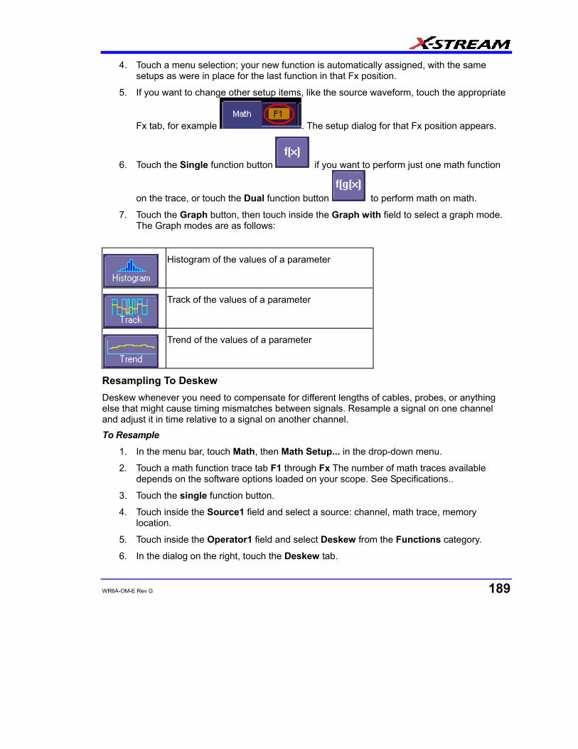
WR6A-OM-E Rev G 189
4. Touch a menu selection; your new function is automatically assigned, with the same setups as were in place for the last function in that Fx position.
5. If you want to change other setup items, like the source waveform, touch the appropriate
Fx tab, for example . The setup dialog for that Fx position appears.
6. Touch the Single function button if you want to perform just one math function
on the trace, or touch the Dual function button to perform math on math.
7. Touch the Graph button, then touch inside the Graph with field to select a graph mode. The Graph modes are as follows:
Histogram of the values of a parameter
Track of the values of a parameter
Trend of the values of a parameter
Resampling To Deskew Deskew whenever you need to compensate for different lengths of cables, probes, or anything else that might cause timing mismatches between signals. Resample a signal on one channel and adjust it in time relative to a signal on another channel. To Resample
1. In the menu bar, touch Math, then Math Setup... in the drop-down menu.
2. Touch a math function trace tab F1 through Fx The number of math traces available depends on the software options loaded on your scope. See Specifications..
3. Touch the single function button.
4. Touch inside the Source1 field and select a source: channel, math trace, memory location.
5. Touch inside the Operator1 field and select Deskew from the Functions category.
6. In the dialog on the right, touch the Deskew tab.
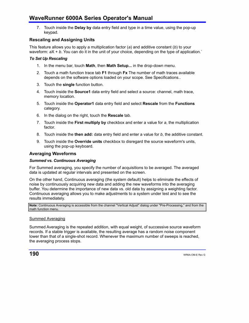
WaveRunner 6000A Series Operator's Manual
190 WR6A-OM-E Rev G
7. Touch inside the Delay by data entry field and type in a time value, using the pop-up keypad.
Rescaling and Assigning Units This feature allows you to apply a multiplication factor (a) and additive constant (b) to your waveform: aX + b. You can do it in the unit of your choice, depending on the type of application.` To Set Up Rescaling
1. In the menu bar, touch Math, then Math Setup... in the drop-down menu.
2. Touch a math function trace tab F1 through Fx The number of math traces available depends on the software options loaded on your scope. See Specifications..
3. Touch the single function button.
4. Touch inside the Source1 data entry field and select a source: channel, math trace, memory location.
5. Touch inside the Operator1 data entry field and select Rescale from the Functions category.
6. In the dialog on the right, touch the Rescale tab.
7. Touch inside the First multiply by checkbox and enter a value for a, the multiplication factor.
8. Touch inside the then add: data entry field and enter a value for b, the additive constant.
9. Touch inside the Override units checkbox to disregard the source waveform's units, using the pop-up keyboard.
Averaging Waveforms Summed vs. Continuous Averaging
For Summed averaging, you specify the number of acquisitions to be averaged. The averaged data is updated at regular intervals and presented on the screen.
On the other hand, Continuous averaging (the system default) helps to eliminate the effects of noise by continuously acquiring new data and adding the new waveforms into the averaging buffer. You determine the importance of new data vs. old data by assigning a weighting factor. Continuous averaging allows you to make adjustments to a system under test and to see the results immediately. Note: Continuous Averaging is accessible from the channel "Vertical Adjust" dialog under "Pre-Processing," and from the math function menu.
Summed Averaging
Summed Averaging is the repeated addition, with equal weight, of successive source waveform records. If a stable trigger is available, the resulting average has a random noise component lower than that of a single-shot record. Whenever the maximum number of sweeps is reached, the averaging process stops.

WR6A-OM-E Rev G 191
An even larger number of records can be accumulated simply by changing the number in the dialog. However, the other parameters must be left unchanged or a new averaging calculation will be started. You can pause the averaging by changing the trigger mode from NORM/AUTO to STOP. The instrument resumes averaging when you change the trigger mode back to NORM/AUTO.
You can reset the accumulated average by pushing the CLEAR SWEEPS button or by changing an acquisition parameter such as input gain, offset, coupling, trigger condition, timebase, or bandwidth limit. The number of current averaged waveforms of the function, or its zoom, is shown in the acquisition status dialog. When summed averaging is performed, the display is updated at a reduced rate to increase the averaging speed (points and events per second).
Continuous Averaging
Continuous Averaging, the default setting, is the repeated addition, with unequal weight, of successive source waveforms. It is particularly useful for reducing noise on signals that drift very slowly in time or amplitude. The most recently acquired waveform has more weight than all the previously acquired ones: the continuous average is dominated by the statistical fluctuations of the most recently acquired waveform. The weight of ‘old’ waveforms in the continuous average gradually tends to zero (following an exponential rule) at a rate that decreases as the weight increases.
The formula for continuous averaging is
new average = (new data + weight * old average)/(weight + 1)
This is also the formula used to compute summed averaging. But by setting a "sweeps" value, you establish a fixed weight that is assigned to the old average once the number of "sweeps" is reached. For example, for a sweeps (weight) value of 4:
1st sweep (no old average yet): new average = (new data +0 * old average)/(0 + 1) = new data only
2nd sweep: new average = (new data + 1*old average)/(1 + 1) = 1/2 new data +1/2 old average
3rd sweep: new average = (new data + 2 * old average)/(2 + 1) = 1/3 new data + 2/3 old average
4th sweep: new average = (new data + 3 * old average)/(3 + 1) = 1/4 new data + 3/4 old average
5th sweep: new average = (new data + 4 * old average)/(4 + 1) = 1/5 new data + 4/5 old average
6th sweep: new average = (new data + 4 * old average)/(4 + 1) = 1/5 new data + 4/5 old average
7th sweep: new average = (new data + 4 * old average)/(4 + 1) = 1/5 new data + 4/5 old average
In this way, for sweeps > 4 the importance of the old average begins to decrease exponentially.

WaveRunner 6000A Series Operator's Manual
192 WR6A-OM-E Rev G
Note: The number of sweeps used to compute the average will be displayed in the bottom line of the trace descriptor label:
To Set Up Continuous Averaging
1. In the menu bar, touch Math, then Math Setup... in the drop-down menu.
2. Select a function tab from F1 through Fx The number of math traces available depends on the software options loaded on your scope. See Specifications..
3. Touch inside the Source1 field and select a source waveform from the pop-up menu.
4. Touch inside the Operator1 field and select Average from the Select Math Operator menu.
5. Touch the Average tab in the dialog to the right of the "Fx" dialog, touch the Continuous button.
6. Touch inside the Sweeps data entry field and enter a value using the pop-up keypad. The valid range is 1 to 1,000,000 sweeps.
To Set Up Summed Averaging
1. In the menu bar, touch Math, then Math Setup... in the drop-down menu.
2. Select a function tab from F1 through Fx The number of math traces available depends on the software options loaded on your scope. See Specifications..
3. Touch inside the Source1 field and select a source waveform from the pop-up menu.
4. Touch inside the Operator1 field and select Average from the Select Math Operator menu.
5. Touch the Average tab in the dialog to the right of the "Fx" dialog, then touch the Summed button.
6. Touch inside the Sweeps data entry field and type in a value using the pop-up keypad. The valid range is 1 to 1,000,000 sweeps.
Enhanced Resolution ERES (Enhanced Resolution) filtering increases vertical resolution, allowing you to distinguish closely spaced voltage levels. The functioning of the instrument's ERES is similar to smoothing the signal with a simple, moving-average filter. However, it is more efficient concerning bandwidth and pass-band filtering. Use ERES on single-shot waveforms, or where the data record is slowly repetitive (when you cannot use averaging). Use it to reduce noise when your signal is noticeably noisy, but you do not need to perform noise measurements. Also use it when you perform high-precision voltage measurements: zooming with high vertical gain, for example.
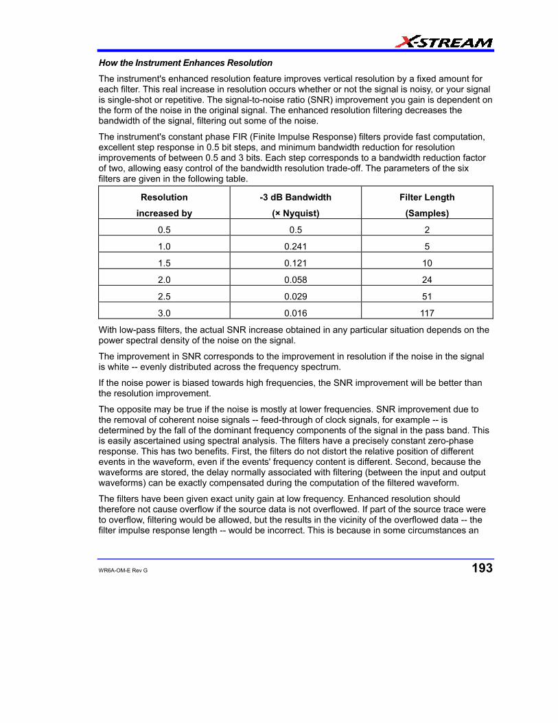
WR6A-OM-E Rev G 193
How the Instrument Enhances Resolution
The instrument's enhanced resolution feature improves vertical resolution by a fixed amount for each filter. This real increase in resolution occurs whether or not the signal is noisy, or your signal is single-shot or repetitive. The signal-to-noise ratio (SNR) improvement you gain is dependent on the form of the noise in the original signal. The enhanced resolution filtering decreases the bandwidth of the signal, filtering out some of the noise.
The instrument's constant phase FIR (Finite Impulse Response) filters provide fast computation, excellent step response in 0.5 bit steps, and minimum bandwidth reduction for resolution improvements of between 0.5 and 3 bits. Each step corresponds to a bandwidth reduction factor of two, allowing easy control of the bandwidth resolution trade-off. The parameters of the six filters are given in the following table.
Resolution
increased by
-3 dB Bandwidth
(× Nyquist)
Filter Length
(Samples)
0.5 0.5 2
1.0 0.241 5
1.5 0.121 10
2.0 0.058 24
2.5 0.029 51
3.0 0.016 117
With low-pass filters, the actual SNR increase obtained in any particular situation depends on the power spectral density of the noise on the signal.
The improvement in SNR corresponds to the improvement in resolution if the noise in the signal is white -- evenly distributed across the frequency spectrum.
If the noise power is biased towards high frequencies, the SNR improvement will be better than the resolution improvement.
The opposite may be true if the noise is mostly at lower frequencies. SNR improvement due to the removal of coherent noise signals -- feed-through of clock signals, for example -- is determined by the fall of the dominant frequency components of the signal in the pass band. This is easily ascertained using spectral analysis. The filters have a precisely constant zero-phase response. This has two benefits. First, the filters do not distort the relative position of different events in the waveform, even if the events' frequency content is different. Second, because the waveforms are stored, the delay normally associated with filtering (between the input and output waveforms) can be exactly compensated during the computation of the filtered waveform.
The filters have been given exact unity gain at low frequency. Enhanced resolution should therefore not cause overflow if the source data is not overflowed. If part of the source trace were to overflow, filtering would be allowed, but the results in the vicinity of the overflowed data -- the filter impulse response length -- would be incorrect. This is because in some circumstances an
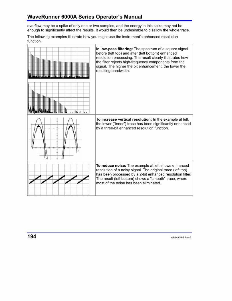
WaveRunner 6000A Series Operator's Manual
194 WR6A-OM-E Rev G
overflow may be a spike of only one or two samples, and the energy in this spike may not be enough to significantly affect the results. It would then be undesirable to disallow the whole trace.
The following examples illustrate how you might use the instrument's enhanced resolution function.
In low-pass filtering: The spectrum of a square signal before (left top) and after (left bottom) enhanced resolution processing. The result clearly illustrates how the filter rejects high-frequency components from the signal. The higher the bit enhancement, the lower the resulting bandwidth.
To increase vertical resolution: In the example at left, the lower ("inner") trace has been significantly enhanced by a three-bit enhanced resolution function.
To reduce noise: The example at left shows enhanced resolution of a noisy signal. The original trace (left top) has been processed by a 2-bit enhanced resolution filter. The result (left bottom) shows a "smooth" trace, where most of the noise has been eliminated.
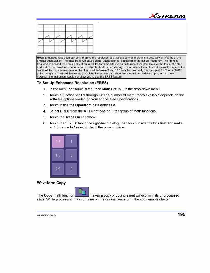
WR6A-OM-E Rev G 195
Note: Enhanced resolution can only improve the resolution of a trace; it cannot improve the accuracy or linearity of the original quantization. The pass-band will cause signal attenuation for signals near the cut-off frequency. The highest frequencies passed may be slightly attenuated. Perform the filtering on finite record lengths. Data will be lost at the start and end of the waveform: the trace will be slightly shorter after filtering. The number of samples lost is exactly equal to the length of the impulse response of the filter used: between 2 and 117 samples. Normally this loss (just 0.2 % of a 50,000 point trace) is not noticed. However, you might filter a record so short there would be no data output. In that case, however, the instrument would not allow you to use the ERES feature.
To Set Up Enhanced Resolution (ERES) 1. In the menu bar, touch Math, then Math Setup... in the drop-down menu.
2. Touch a function tab F1 through Fx The number of math traces available depends on the software options loaded on your scope. See Specifications..
3. Touch inside the Operator1 data entry field.
4. Select ERES from the All Functions or Filter group of Math functions.
5. Touch the Trace On checkbox.
6. Touch the "ERES" tab in the right-hand dialog, then touch inside the bits field and make an "Enhance by" selection from the pop-up menu:
.
Waveform Copy
The Copy math function makes a copy of your present waveform in its unprocessed state. While processing may continue on the original waveform, the copy enables faster

WaveRunner 6000A Series Operator's Manual
196 WR6A-OM-E Rev G
throughput in some cases by preserving the original data. That is, no calculations need to be undone on the copy before additional math can be calculated.
This benefit of faster throughput, however, comes at the expense of memory usage.
Waveform Sparser
The Sparse math function allows you to thin out an incoming waveform by skipping points at regular intervals, and by starting acquisition at a particular "offset" (point). The Sparsing factor specifies the number of sample points to reduce the input waveform by. A sparsing factor of 4, for example, tells the scope to retain only one out of every 4 samples. A Sparsing offset of 3, on the other hand, tells the scope to begin on the third sample, then skip the number of samples specified by the sparsing factor (4). In this way, the sample rate is effectively reduced.
For the sparsing factor (interval), you can set a value from 1 to 1,000,000 points. For the sparsing offset you can set a value from 0 to 999,999.
Note: The maximum sparsing offset that can be entered for any sparsing factor equals Sparsing Factor 1.
To Set Up Waveform Sparser
1. In the menu bar, touch Math, then Math setup... in the drop-down menu.
2. Touch the tab for the function (F1 to Fx The number of math traces available depends on the software options loaded on your scope. See specifications.) you want to assign the Sparse operation to.
3. Touch inside the Source1 field and select an input waveform.
4. Touch inside the Operator1 field and select Sparse from the Select Math Operator menu.
5. Touch inside the Sparsing factor field and enter a value, using the pop-up keypad.
6. Touch inside the Sparsing offset field and enter a value, using the pop-up keypad.
Interpolation Linear interpolation, which inserts a straight line between sample point, is best used to reconstruct straight-edged signals such as square waves. (Sinx)/x interpolation, on the other hand, is suitable for reconstructing curved or irregular waveshapes, especially when the sampling rate is 3 to 5 times the system bandwidth. The instrument also gives you a choice of Cubic interpolation.
For each method, you can select a factor from 2 to 50 points by which to interpolate (upsample). To Set Up Interpolation
1. In the menu bar, touch Math, then Math setup... in the drop-down menu.
2. Touch the tab for the function (F1 to Fx The number of math traces available depends on the software options loaded on your scope. See Specifications.) you want to assign the Interpolate operation to.

WR6A-OM-E Rev G 197
3. Touch inside the Source1 field and select an input waveform.
4. Touch inside the Operator1 field, then touch the Filter button in the Select Math Operator menu.
5. Select Interpolate from the Filter submenu.
6. Touch the "Interpolate" tab in the mini setup dialog to the right of the main dialog.
7. Touch inside the Algorithm field and select an interpolation type.
8. Touch inside the Upsample by Upsampling is the factor by which sampling is increased. field and enter a value, using the pop-up numeric keypad, if you want to enter a specific value. Otherwise, use the Up/Down buttons to increment the displayed value in a 1-2-5 sequence.
WaveRunner 6000A Series Operator's Manual
198 WR6A-OM-E Rev G
FFT Why Use FFT? For a large class of signals, you can gain greater insight by looking at spectral representation rather than time description. Signals encountered in the frequency response of amplifiers, oscillator phase noise and those in mechanical vibration analysis, for example, are easier to observe in the frequency domain.
If sampling is done at a rate fast enough to faithfully approximate the original waveform (usually five times the highest frequency component in the signal), the resulting discrete data series will uniquely describe the analog signal. This is of particular value when dealing with transient signals because, unlike FFT, conventional swept spectrum analyzers cannot handle them.
Spectral analysis theory assumes that the signal for transformation is of infinite duration. Since no physical signal can meet this condition, a useful assumption for reconciling theory and practice is to view the signal as consisting of an infinite series of replicas of itself. These replicas are multiplied by a rectangular window (the display grid) that is zero outside of the observation grid.
An FFT operation on an N-point time domain signal can be compared to passing the signal through a comb filter consisting of a bank of N/2 filters. All the filters have the same shape and width and are centered at N/2 discrete frequencies. Each filter collects the signal energy that falls into the immediate neighborhood of its center frequency. Thus it can be said that there are N/2 frequency bins. The distance in Hz between the center frequencies of two neighboring bins is always the same: Delta f.
Power (Density) Spectrum Because of the linear scale used to show magnitudes, lower amplitude components are often hidden by larger components. In addition to the functions offering magnitude and phase representations, the FFT option offers power density and power spectrum density functions. These latter functions are even better suited for characterizing spectra. The power spectrum (V2) is the square of the magnitude spectrum (0 dBm corresponds to voltage equivalent to 1 mW into 50 ohms.) This is the representation of choice for signals containing isolated peaks — periodic signals, for instance.
The power density spectrum (V2/Hz) is the power spectrum divided by the equivalent noise bandwidth of the filter associated with the FFT calculation. This is best employed for characterizing broadband signals such as noise.
Memory for FFT
The amount of acquisition memory available will determine the maximum range (Nyquist frequency) over which signal components can be observed. Consider the problem of determining the length of the observation window and the size of the acquisition buffer if a Nyquist rate of 500 MHz and a resolution of 10 kHz are required. To obtain a resolution of 10 kHz, the acquisition time must be at least:
T = 1/Delta f = 1/10 kHz = 100 ms

WR6A-OM-E Rev G 199
For a digital oscilloscope with a memory of 100 kB, the highest frequency that can be analyzed is:
Delta f x N/2 = 10 kHz x 100 kB/2 = 500 MHz
FFT Pitfalls to Avoid Take care to ensure that signals are correctly acquired: improper waveform positioning within the observation window produces a distorted spectrum. The most common distortions can be traced to insufficient sampling, edge discontinuities, windowing or the "picket fence" effect.
Because the FFT acts like a bank of band-pass filters centered at multiples of the frequency resolution, components that are not exact multiples of that frequency will fall within two consecutive filters. This results in an attenuation of the true amplitude of these components.
Picket Fence and Scallop The highest point in the spectrum can be 3.92 dB lower when the source frequency is halfway between two discrete frequencies. This variation in spectrum magnitude is the picket fence effect. The corresponding attenuation loss is referred to as scallop loss. LeCroy scopes automatically correct for the scallop effect, ensuring that the magnitude of the spectra lines correspond to their true values in the time domain.
If a signal contains a frequency component above Nyquist, the spectrum will be aliased, meaning that the frequencies will be folded back and spurious. Spotting aliased frequencies is often difficult, as the aliases may ride on top of real harmonics. A simple way of checking is to modify the sample rate and observe whether the frequency distribution changes.
Leakage FFT assumes that the signal contained within the time grid is replicated endlessly outside the observation window. Therefore if the signal contains discontinuities at its edges, pseudo-frequencies will appear in the spectral domain, distorting the real spectrum. When the start and end phase of the signal differ, the signal frequency falls within two frequency cells, broadening the spectrum.
The broadening of the base, stretching out in many neighboring bins, is termed leakage. Cures for this are to ensure that an integral number of periods is contained within the display grid or that no discontinuities appear at the edges. Another is to use a window function to smooth the edges of the signal.
Choosing a Window The choice of a spectral window is dictated by the signal’s characteristics. Weighting functions control the filter response shape, and affect noise bandwidth as well as side lobe levels. Ideally, the main lobe should be as narrow and flat as possible to effectively discriminate all spectral components, while all side lobes should be infinitely attenuated. The window type defines the bandwidth and shape of the equivalent filter to be used in the FFT processing.
In the same way as one would choose a particular camera lens for taking a picture, some experimenting is generally necessary to determine which window is most suitable. However, the following general guidelines should help.
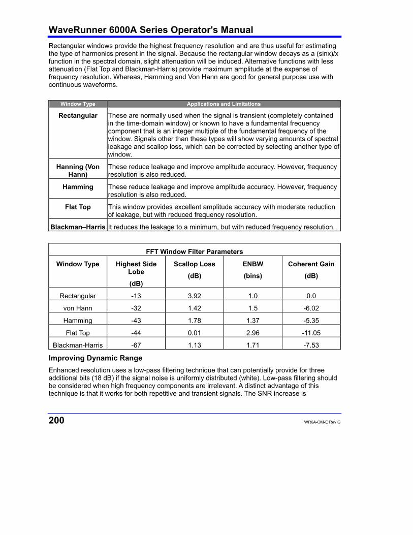
WaveRunner 6000A Series Operator's Manual
200 WR6A-OM-E Rev G
Rectangular windows provide the highest frequency resolution and are thus useful for estimating the type of harmonics present in the signal. Because the rectangular window decays as a (sinx)/x function in the spectral domain, slight attenuation will be induced. Alternative functions with less attenuation (Flat Top and Blackman-Harris) provide maximum amplitude at the expense of frequency resolution. Whereas, Hamming and Von Hann are good for general purpose use with continuous waveforms.
Window Type Applications and Limitations
Rectangular These are normally used when the signal is transient (completely contained in the time-domain window) or known to have a fundamental frequency component that is an integer multiple of the fundamental frequency of the window. Signals other than these types will show varying amounts of spectral leakage and scallop loss, which can be corrected by selecting another type of window.
Hanning (Von Hann)
These reduce leakage and improve amplitude accuracy. However, frequency resolution is also reduced.
Hamming These reduce leakage and improve amplitude accuracy. However, frequency resolution is also reduced.
Flat Top This window provides excellent amplitude accuracy with moderate reduction of leakage, but with reduced frequency resolution.
Blackman–Harris It reduces the leakage to a minimum, but with reduced frequency resolution.
FFT Window Filter Parameters
Window Type Highest Side Lobe
(dB)
Scallop Loss
(dB)
ENBW
(bins)
Coherent Gain
(dB)
Rectangular -13 3.92 1.0 0.0
von Hann -32 1.42 1.5 -6.02
Hamming -43 1.78 1.37 -5.35
Flat Top -44 0.01 2.96 -11.05
Blackman-Harris -67 1.13 1.71 -7.53
Improving Dynamic Range Enhanced resolution uses a low-pass filtering technique that can potentially provide for three additional bits (18 dB) if the signal noise is uniformly distributed (white). Low-pass filtering should be considered when high frequency components are irrelevant. A distinct advantage of this technique is that it works for both repetitive and transient signals. The SNR increase is
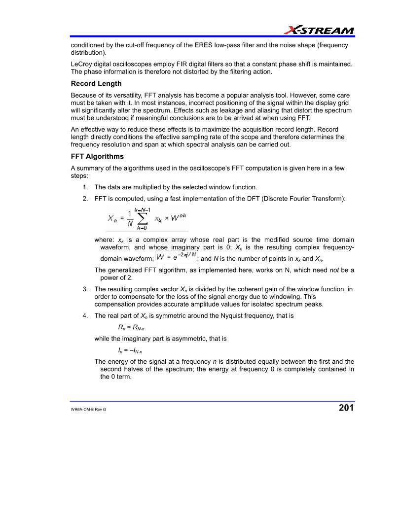
WR6A-OM-E Rev G 201
conditioned by the cut-off frequency of the ERES low-pass filter and the noise shape (frequency distribution).
LeCroy digital oscilloscopes employ FIR digital filters so that a constant phase shift is maintained. The phase information is therefore not distorted by the filtering action.
Record Length Because of its versatility, FFT analysis has become a popular analysis tool. However, some care must be taken with it. In most instances, incorrect positioning of the signal within the display grid will significantly alter the spectrum. Effects such as leakage and aliasing that distort the spectrum must be understood if meaningful conclusions are to be arrived at when using FFT.
An effective way to reduce these effects is to maximize the acquisition record length. Record length directly conditions the effective sampling rate of the scope and therefore determines the frequency resolution and span at which spectral analysis can be carried out.
FFT Algorithms A summary of the algorithms used in the oscilloscope's FFT computation is given here in a few steps:
1. The data are multiplied by the selected window function.
2. FFT is computed, using a fast implementation of the DFT (Discrete Fourier Transform):
where: xk is a complex array whose real part is the modified source time domain
waveform, and whose imaginary part is 0; Xn is the resulting complex frequency-
domain waveform; ; and N is the number of points in xk and Xn.
The generalized FFT algorithm, as implemented here, works on N, which need not be a power of 2.
3. The resulting complex vector Xn is divided by the coherent gain of the window function, in order to compensate for the loss of the signal energy due to windowing. This compensation provides accurate amplitude values for isolated spectrum peaks.
4. The real part of Xn is symmetric around the Nyquist frequency, that is
Rn = RN-n
while the imaginary part is asymmetric, that is
In = –IN-n
The energy of the signal at a frequency n is distributed equally between the first and the second halves of the spectrum; the energy at frequency 0 is completely contained in the 0 term.
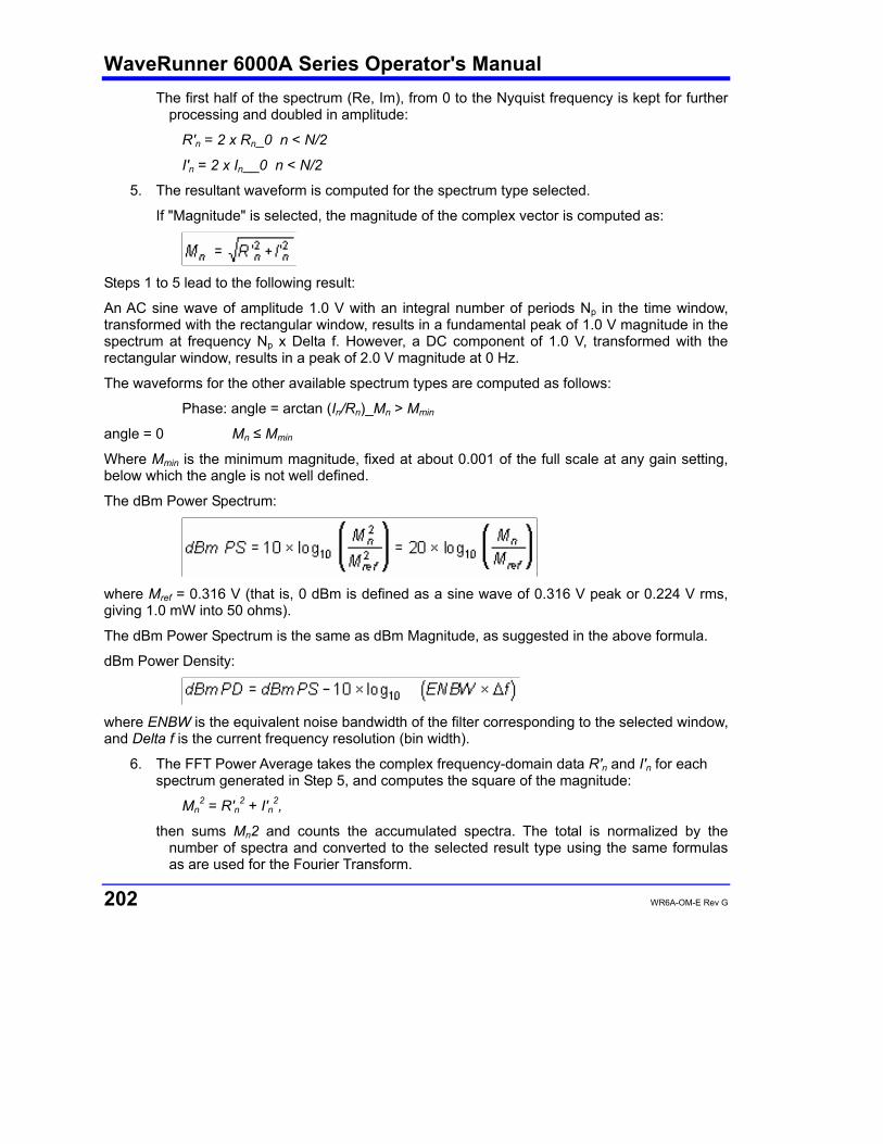
WaveRunner 6000A Series Operator's Manual
202 WR6A-OM-E Rev G
The first half of the spectrum (Re, Im), from 0 to the Nyquist frequency is kept for further processing and doubled in amplitude:
R'n = 2 x Rn_0 n < N/2
I'n = 2 x In__0 n < N/2
5. The resultant waveform is computed for the spectrum type selected.
If "Magnitude" is selected, the magnitude of the complex vector is computed as:
Steps 1 to 5 lead to the following result:
An AC sine wave of amplitude 1.0 V with an integral number of periods Np in the time window, transformed with the rectangular window, results in a fundamental peak of 1.0 V magnitude in the spectrum at frequency Np x Delta f. However, a DC component of 1.0 V, transformed with the rectangular window, results in a peak of 2.0 V magnitude at 0 Hz.
The waveforms for the other available spectrum types are computed as follows:
Phase: angle = arctan (In/Rn)_Mn > Mmin
angle = 0 Mn ≤ Mmin
Where Mmin is the minimum magnitude, fixed at about 0.001 of the full scale at any gain setting, below which the angle is not well defined.
The dBm Power Spectrum:
where Mref = 0.316 V (that is, 0 dBm is defined as a sine wave of 0.316 V peak or 0.224 V rms, giving 1.0 mW into 50 ohms).
The dBm Power Spectrum is the same as dBm Magnitude, as suggested in the above formula.
dBm Power Density:
where ENBW is the equivalent noise bandwidth of the filter corresponding to the selected window, and Delta f is the current frequency resolution (bin width).
6. The FFT Power Average takes the complex frequency-domain data R'n and I'n for each spectrum generated in Step 5, and computes the square of the magnitude:
Mn2 = R'n2 + I'n2,
then sums Mn2 and counts the accumulated spectra. The total is normalized by the number of spectra and converted to the selected result type using the same formulas as are used for the Fourier Transform.
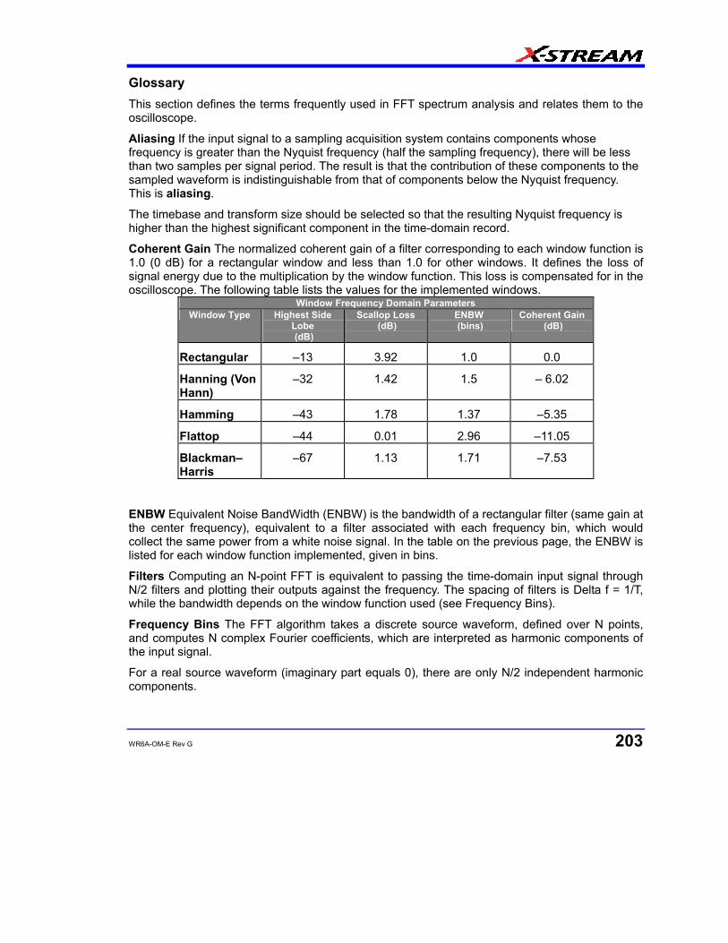
WR6A-OM-E Rev G 203
Glossary This section defines the terms frequently used in FFT spectrum analysis and relates them to the oscilloscope.
Aliasing If the input signal to a sampling acquisition system contains components whose frequency is greater than the Nyquist frequency (half the sampling frequency), there will be less than two samples per signal period. The result is that the contribution of these components to the sampled waveform is indistinguishable from that of components below the Nyquist frequency. This is aliasing.
The timebase and transform size should be selected so that the resulting Nyquist frequency is higher than the highest significant component in the time-domain record.
Coherent Gain The normalized coherent gain of a filter corresponding to each window function is 1.0 (0 dB) for a rectangular window and less than 1.0 for other windows. It defines the loss of signal energy due to the multiplication by the window function. This loss is compensated for in the oscilloscope. The following table lists the values for the implemented windows.
Window Frequency Domain Parameters Window Type Highest Side
Lobe (dB)
Scallop Loss (dB)
ENBW (bins)
Coherent Gain (dB)
Rectangular –13 3.92 1.0 0.0
Hanning (Von Hann)
–32 1.42 1.5 – 6.02
Hamming –43 1.78 1.37 –5.35
Flattop –44 0.01 2.96 –11.05
Blackman–Harris
–67 1.13 1.71 –7.53
ENBW Equivalent Noise BandWidth (ENBW) is the bandwidth of a rectangular filter (same gain at the center frequency), equivalent to a filter associated with each frequency bin, which would collect the same power from a white noise signal. In the table on the previous page, the ENBW is listed for each window function implemented, given in bins.
Filters Computing an N-point FFT is equivalent to passing the time-domain input signal through N/2 filters and plotting their outputs against the frequency. The spacing of filters is Delta f = 1/T, while the bandwidth depends on the window function used (see Frequency Bins).
Frequency Bins The FFT algorithm takes a discrete source waveform, defined over N points, and computes N complex Fourier coefficients, which are interpreted as harmonic components of the input signal.
For a real source waveform (imaginary part equals 0), there are only N/2 independent harmonic components.
WaveRunner 6000A Series Operator's Manual
204 WR6A-OM-E Rev G
An FFT corresponds to analyzing the input signal with a bank of N/2 filters, all having the same shape and width, and centered at N/2 discrete frequencies. Each filter collects the signal energy that falls into the immediate neighborhood of its center frequency. Thus it can be said that there are N/2 "frequency bins."
The distance in hertz between the center frequencies of two neighboring bins is always:
Delta f = 1/T
where T is the duration of the time-domain record in seconds.
The width of the main lobe of the filter centered at each bin depends on the window function used. The rectangular window has a nominal width at 1.0 bin. Other windows have wider main lobes (see table).
Frequency Range The range of frequencies computed and displayed is 0 Hz (displayed at the left-hand edge of the screen) to the Nyquist frequency (at the rightmost edge of the trace).
Frequency Resolution In a simple sense, the frequency resolution is equal to the bin width Delta f. That is, if the input signal changes its frequency by Delta f, the corresponding spectrum peak will be displaced by Df. For smaller changes of frequency, only the shape of the peak will change.
However, the effective frequency resolution (that is, the ability to resolve two signals whose frequencies are almost the same) is further limited by the use of window functions. The ENBW value of all windows other than the rectangular is greater than Delta f and the bin width. The table of Window Frequency-Domain Parameters lists the ENBW values for the implemented windows.
Leakage In the power spectrum of a sine wave with an integral number of periods in the (rectangular) time window (that is, the source frequency equals one of the bin frequencies), the spectrum contains a sharp component whose value accurately reflects the source waveform's amplitude. For intermediate input frequencies this spectral component has a lower and broader peak.
The broadening of the base of the peak, stretching out into many neighboring bins, is termed leakage. It is due to the relatively high side lobes of the filter associated with each frequency bin.
The filter side lobes and the resulting leakage are reduced when one of the available window functions is applied. The best reduction is provided by the Blackman-Harris and Flattop windows. However, this reduction is offset by a broadening of the main lobe of the filter.
Number of Points The FFT is computed over the number of points (Transform Size) whose upper bounds are the source number of points, and by the maximum number of points selected in the menu. The FFT generates spectra of N/2 output points.
Nyquist Frequency The Nyquist frequency is equal to one half of the effective sampling frequency (after the decimation): Delta f x N/2.
Picket Fence Effect If a sine wave has a whole number of periods in the time domain record, the power spectrum obtained with a rectangular window will have a sharp peak, corresponding exactly to the frequency and amplitude of the sine wave. Otherwise the spectrum peak with a rectangular window will be lower and broader.
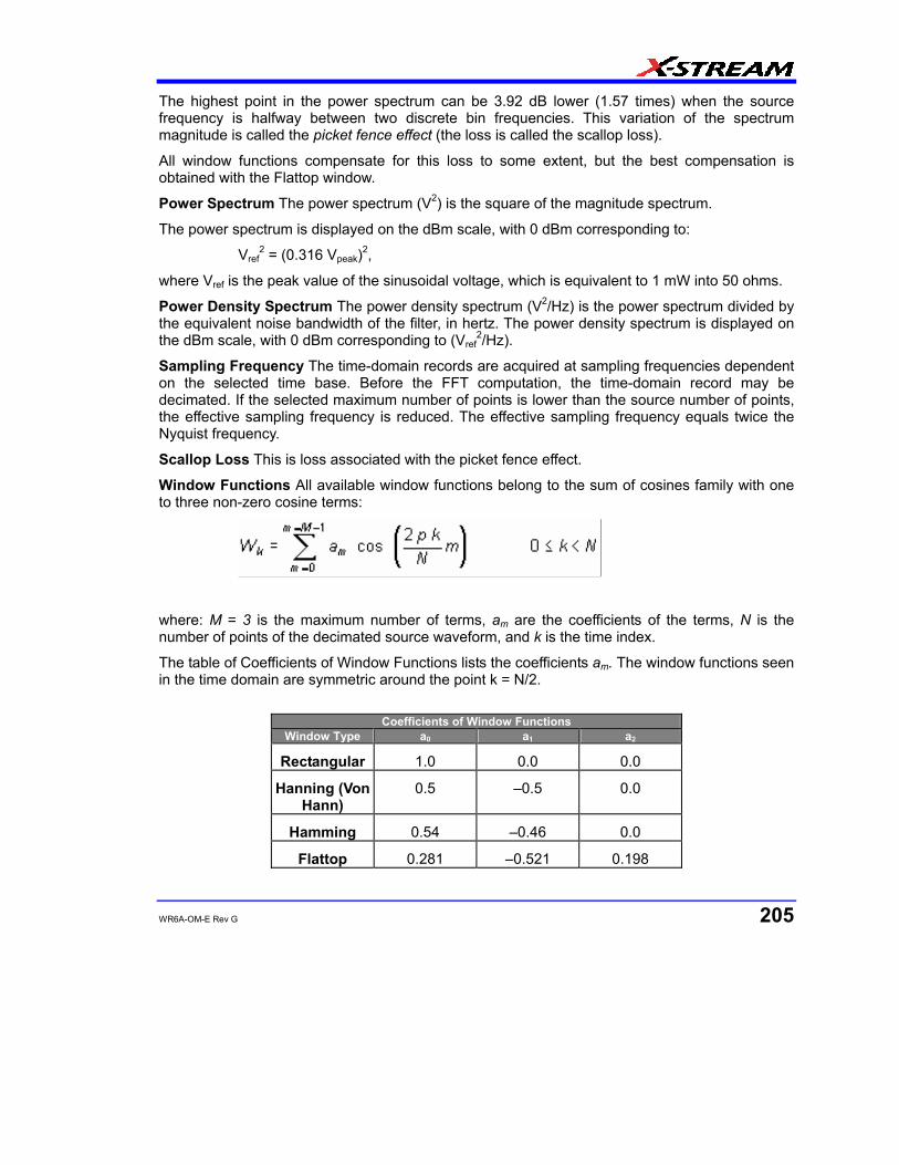
WR6A-OM-E Rev G 205
The highest point in the power spectrum can be 3.92 dB lower (1.57 times) when the source frequency is halfway between two discrete bin frequencies. This variation of the spectrum magnitude is called the picket fence effect (the loss is called the scallop loss).
All window functions compensate for this loss to some extent, but the best compensation is obtained with the Flattop window.
Power Spectrum The power spectrum (V2) is the square of the magnitude spectrum.
The power spectrum is displayed on the dBm scale, with 0 dBm corresponding to:
Vref2 = (0.316 Vpeak)2,
where Vref is the peak value of the sinusoidal voltage, which is equivalent to 1 mW into 50 ohms.
Power Density Spectrum The power density spectrum (V2/Hz) is the power spectrum divided by the equivalent noise bandwidth of the filter, in hertz. The power density spectrum is displayed on the dBm scale, with 0 dBm corresponding to (Vref
2/Hz).
Sampling Frequency The time-domain records are acquired at sampling frequencies dependent on the selected time base. Before the FFT computation, the time-domain record may be decimated. If the selected maximum number of points is lower than the source number of points, the effective sampling frequency is reduced. The effective sampling frequency equals twice the Nyquist frequency.
Scallop Loss This is loss associated with the picket fence effect.
Window Functions All available window functions belong to the sum of cosines family with one to three non-zero cosine terms:
where: M = 3 is the maximum number of terms, am are the coefficients of the terms, N is the number of points of the decimated source waveform, and k is the time index.
The table of Coefficients of Window Functions lists the coefficients am. The window functions seen in the time domain are symmetric around the point k = N/2.
Coefficients of Window Functions
Window Type a0 a1 a2
Rectangular 1.0 0.0 0.0
Hanning (Von Hann)
0.5 –0.5 0.0
Hamming 0.54 –0.46 0.0
Flattop 0.281 –0.521 0.198

WaveRunner 6000A Series Operator's Manual
206 WR6A-OM-E Rev G
Blackman–Harris
0.423 –0.497 0.079
FFT Setup To Set Up an FFT
1. In the menu bar touch Math, then Math Setup... in the drop-down menu.
2. Touch a Math function trace button: F1 through Fx The number of math traces available depends on the software options loaded on your scope. See Specifications.; a pop-up
menu appears. Select FFT from the menu.
3. Touch the Single or Dual (function of a function) button if the FFT is to be of the result of another math operation.
4. Touch inside the Source1 field and select a channel, memory, or math trace on which to perform the FFT.
5. Touch inside the Operator1 field: Select FFT from the pop-up menu if you selected Single function. Select another math function if you selected Dual function. Then touch inside the Operator2 field and select FFT from the pop-up menu.
6. In the right-hand dialog, touch the FFT tab.
7. Choose whether to Truncate1 or Zero-fill2 the trace display.
8. Touch the Suppress DC checkbox if you want to make the DC bin go to zero. Otherwise, leave it unchecked.
9. Touch inside the Output type field, and make a selection from the pop-up menu.
10. Touch inside the Window field, select a window type.
11. Touch inside the Algorithm field and select either Least Prime3 from the pop-up menu.
1 When the FFT transform size does not match the record length, you can truncate the record and perform an FFT on the shorter record. This will increase the resolution bandwidth. 2 Zero-fill is useful when the source data for the FFT comes from a math operation that shortens the record. This is commonly encountered in filtering operations like enhanced resolution. The missing data points are replaced by data values, whose amplitudes are interpolated to fit between the last data point and the first data point in the record. This guarantees that there is not a first-order discontinuity in the filled data. Since the data at the end of the record is "filled" data, it is advisable to select a weighting window other than rectangular to minimize the effect of the fill on the resulting spectrum. 3 The default algorithm is a least primes algorithm that computes FFTs on transform sizes having lengths that can be expressed as factors of 2N*5K. This is very compatible with the record lengths encountered in the oscilloscope, which are often multiples of 1, 2, 4, 5, or 10. or Power of 2 The other choice is a power of two algorithm where the record lengths are
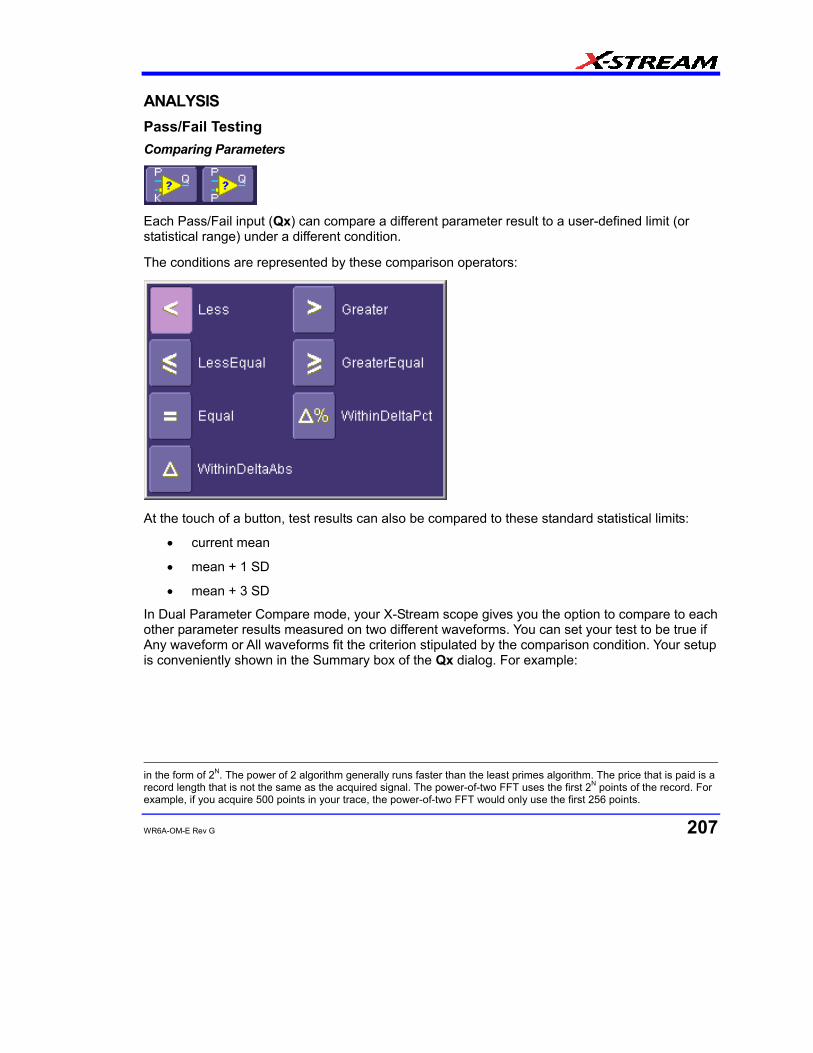
WR6A-OM-E Rev G 207
ANALYSIS Pass/Fail Testing Comparing Parameters
Each Pass/Fail input (Qx) can compare a different parameter result to a user-defined limit (or statistical range) under a different condition.
The conditions are represented by these comparison operators:
At the touch of a button, test results can also be compared to these standard statistical limits:
• current mean
• mean + 1 SD
• mean + 3 SD
In Dual Parameter Compare mode, your X-Stream scope gives you the option to compare to each other parameter results measured on two different waveforms. You can set your test to be true if Any waveform or All waveforms fit the criterion stipulated by the comparison condition. Your setup is conveniently shown in the Summary box of the Qx dialog. For example:
in the form of 2N. The power of 2 algorithm generally runs faster than the least primes algorithm. The price that is paid is a record length that is not the same as the acquired signal. The power-of-two FFT uses the first 2N points of the record. For example, if you acquire 500 points in your trace, the power-of-two FFT would only use the first 256 points.
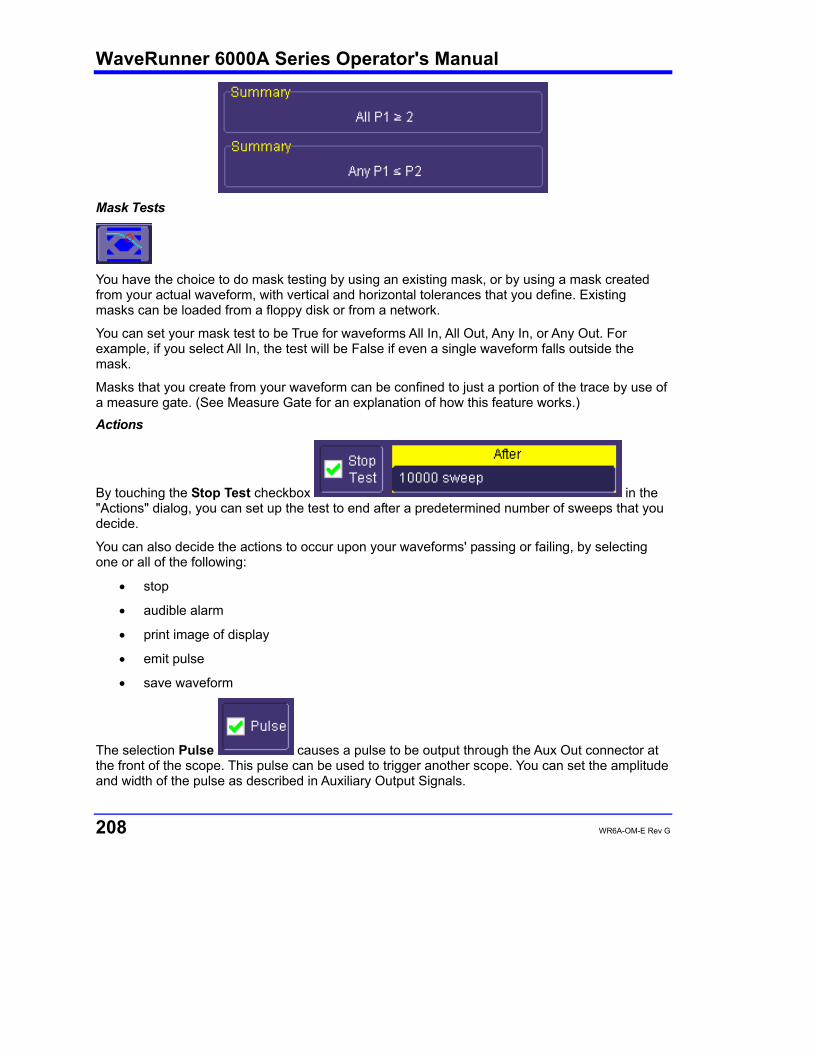
WaveRunner 6000A Series Operator's Manual
208 WR6A-OM-E Rev G
Mask Tests
You have the choice to do mask testing by using an existing mask, or by using a mask created from your actual waveform, with vertical and horizontal tolerances that you define. Existing masks can be loaded from a floppy disk or from a network.
You can set your mask test to be True for waveforms All In, All Out, Any In, or Any Out. For example, if you select All In, the test will be False if even a single waveform falls outside the mask.
Masks that you create from your waveform can be confined to just a portion of the trace by use of a measure gate. (See Measure Gate for an explanation of how this feature works.) Actions
By touching the Stop Test checkbox in the "Actions" dialog, you can set up the test to end after a predetermined number of sweeps that you decide.
You can also decide the actions to occur upon your waveforms' passing or failing, by selecting one or all of the following:
• stop
• audible alarm
• print image of display
• emit pulse
• save waveform
The selection Pulse causes a pulse to be output through the Aux Out connector at the front of the scope. This pulse can be used to trigger another scope. You can set the amplitude and width of the pulse as described in Auxiliary Output Signals.
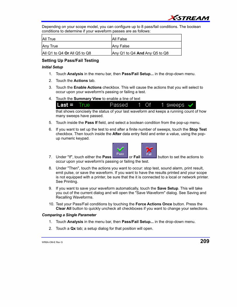
WR6A-OM-E Rev G 209
Depending on your scope model, you can configure up to 8 pass/fail conditions. The boolean conditions to determine if your waveform passes are as follows:
All True All False
Any True Any False
All Q1 to Q4 Or All Q5 to Q8 Any Q1 to Q4 And Any Q5 to Q8
Setting Up Pass/Fail Testing Initial Setup
1. Touch Analysis in the menu bar, then Pass/Fail Setup... in the drop-down menu.
2. Touch the Actions tab.
3. Touch the Enable Actions checkbox. This will cause the actions that you will select to occur upon your waveform's passing or failing a test.
4. Touch the Summary View to enable a line of text
that shows concisely the status of your last waveform and keeps a running count of how many sweeps have passed.
5. Touch inside the Pass If field, and select a boolean condition from the pop-up menu.
6. If you want to set up the test to end after a finite number of sweeps, touch the Stop Test checkbox. Then touch inside the After data entry field and enter a value, using the pop-up numeric keypad.
7. Under "If", touch either the Pass or Fail button to set the actions to occur upon your waveform's passing or failing the test.
8. Under "Then", touch the actions you want to occur: stop test, sound alarm, print result, emit pulse, or save the waveform. If you want to have the results printed and your scope is not equipped with a printer, be sure that the it is connected to a local or network printer. See Printing.
9. If you want to save your waveform automatically, touch the Save Setup. This will take you out of the current dialog and will open the "Save Waveform" dialog. See Saving and Recalling Waveforms.
10. Test your Pass/Fail conditions by touching the Force Actions Once button. Press the Clear All button to quickly uncheck all checkboxes if you want to change your selections.
Comparing a Single Parameter
1. Touch Analysis in the menu bar, then Pass/Fail Setup... in the drop-down menu.
2. Touch a Qx tab; a setup dialog for that position will open.

WaveRunner 6000A Series Operator's Manual
210 WR6A-OM-E Rev G
3. Touch inside the Source1 field and select a source from the pop-up menu.
4. Touch inside the Condition field in the main dialog and select ParamCompare
5. Touch inside the Compare Values field and select All or Any from the pop-up menu
. By selecting All, the test will be true only if every waveform falls within the limit that you will set. By selecting Any, the test will be true if just one waveform falls within the limit.
6. Touch inside the Condition field in the "ParamCompare" mini-dialog and select a math operator from the pop-up menu:
.
7. Touch inside the Limit field and enter a value, using the pop-up numeric keypad. This value takes the dimensions of the parameter that you are testing. For example, if you are
testing a time parameter, the unit is seconds. If you chose either WithinDeltaPct
or WithinDeltaAbs from the Condition menu, you also have the choice of

WR6A-OM-E Rev G 211
setting the limit by means of the statistical buttons at the bottom of the "ParamCompare"
dialog: Comparing Dual Parameters
1. Touch Analysis in the menu bar, then Pass/Fail Setup... in the drop-down menu.
2. Touch a Qx tab; a setup dialog for that position will open.
3. Touch inside the Condition field in the main dialog and select DualParamCompare
.
4. Touch inside the Source1 and Source2 fields and select a source from the pop-up menu.
5. Touch inside the "ParamCompare" mini-dialog field and select a source from the pop-up menu.
6. Touch inside the Compare Values field and select All or Any from the pop-up menu:
. By selecting All, the test will be true only if every waveform falls within the limit that you will set. By selecting Any, the test will be true if just one waveform falls within the limit.
7. Touch inside the Condition field in the "ParamCompare" mini-dialog and select a math operator from the pop-up menu:
.
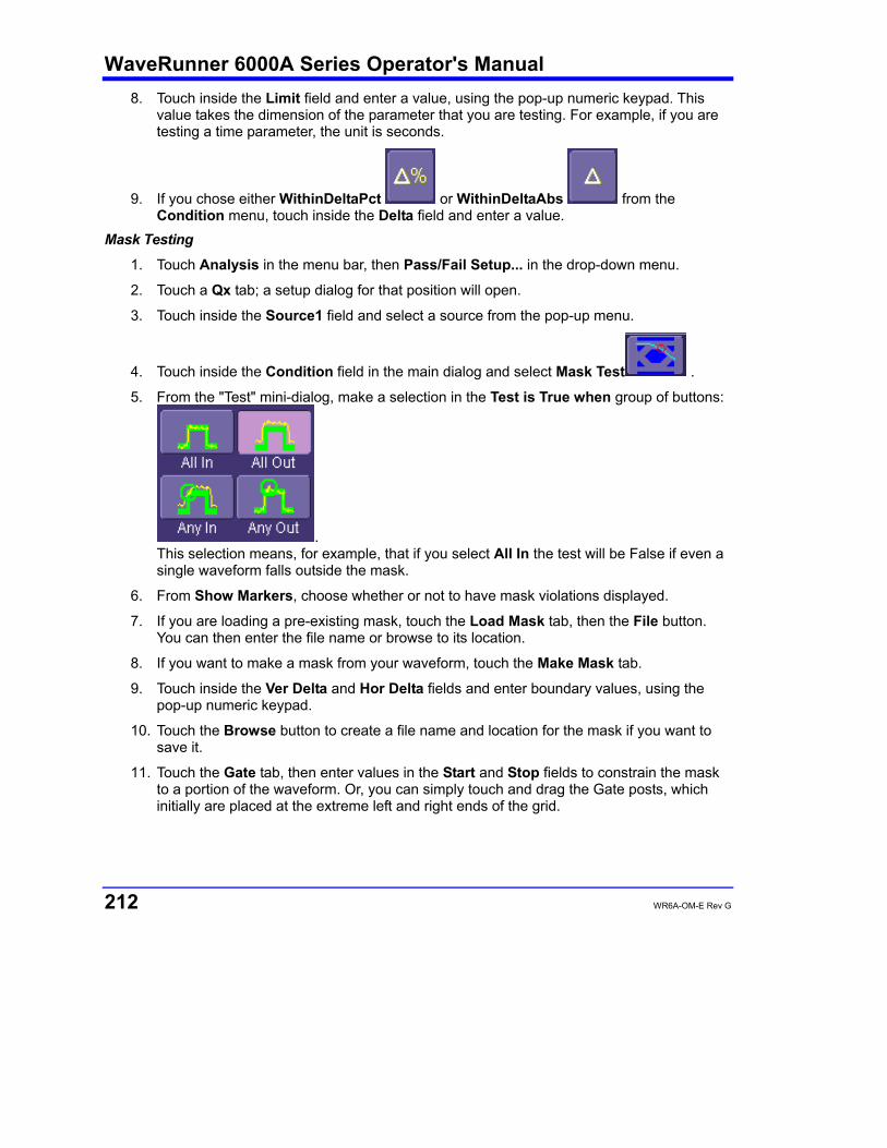
WaveRunner 6000A Series Operator's Manual
212 WR6A-OM-E Rev G
8. Touch inside the Limit field and enter a value, using the pop-up numeric keypad. This value takes the dimension of the parameter that you are testing. For example, if you are testing a time parameter, the unit is seconds.
9. If you chose either WithinDeltaPct or WithinDeltaAbs from the Condition menu, touch inside the Delta field and enter a value.
Mask Testing
1. Touch Analysis in the menu bar, then Pass/Fail Setup... in the drop-down menu.
2. Touch a Qx tab; a setup dialog for that position will open.
3. Touch inside the Source1 field and select a source from the pop-up menu.
4. Touch inside the Condition field in the main dialog and select Mask Test .
5. From the "Test" mini-dialog, make a selection in the Test is True when group of buttons:
. This selection means, for example, that if you select All In the test will be False if even a single waveform falls outside the mask.
6. From Show Markers, choose whether or not to have mask violations displayed.
7. If you are loading a pre-existing mask, touch the Load Mask tab, then the File button. You can then enter the file name or browse to its location.
8. If you want to make a mask from your waveform, touch the Make Mask tab.
9. Touch inside the Ver Delta and Hor Delta fields and enter boundary values, using the pop-up numeric keypad.
10. Touch the Browse button to create a file name and location for the mask if you want to save it.
11. Touch the Gate tab, then enter values in the Start and Stop fields to constrain the mask to a portion of the waveform. Or, you can simply touch and drag the Gate posts, which initially are placed at the extreme left and right ends of the grid.
WR6A-OM-E Rev G 213
UTILITIES Status The status read-only dialog displays system information including serial number, firmware version, and installed software and hardware options. To Access Status Dialog
1. In the menu bar, touch Utilities.
2. Touch the Status tab.
Remote communication The Remote dialog is where you can select a network communication protocol, establish network connections, and configure the Remote Control Assistant log. The choice of communication protocols is limited to TCPIP and GPIB. Note: GPIB is an option and requires a GPIB card to be installed in a card slot at the rear of the scope.
Note: The instrument uses Dynamic Host Configuration Protocol (DHCP) as its addressing protocol. Therefore, it is not necessary to set up an IP address if your network supports DHCP. If it does not, you can assign a static address in the standard Windows 2000 network setup menu.
The Remote Control Assistant monitors communication between your PC and scope when you are operating the instrument remotely. You can log all events, or errors only. This log can be invaluable when you are creating and debugging remote control applications. To Set Up Remote Communication.
1. If you are connecting the scope to a network, first contact your Information Systems administrator. If you are connecting the scope directly to your PC, connect a GPIB or Ethernet cable between them.
2. In the menu bar touch Utilities, then Utilities Setup... in the drop-down menu.
3. Touch the Remote tab.
4. Make a Port selection:TCPIP (transmission control protocol/Internet protocol) or GPIB (general purpose interface bus). If you do not have a GPIB card installed, the GPIB selection will not be accessible.
5. If you are using GPIB, set a GPIB address by touching inside the GPIB Address data entry field and enter an address.
6. Press the Net Connections button; the Windows Network and Dial-up Connections window appears.
7. Touch Make New Connection and use the Windows Network Connection Wizard to make a new connection; or, touch Local Area Connection to reconfigure the scope's connection if it is already connected to the network.
To Configure the Remote Control Assistant Event Log
1. In the menu bar touch Utilities, then Utilities Setup... in the drop-down menu.
WaveRunner 6000A Series Operator's Manual
214 WR6A-OM-E Rev G
2. Touch the Remote tab.
3. Touch inside the Log Mode data entry field.
4. Select Off, Errors Only, or Full Dialog from the pop-up menu.
5. To export the contents of the event log to an ASCII text file, touch the Show Remote Control Log button: the "Event Logs" popup window appears. Touch inside the DestFilename data entry field and enter a file name, using the pop-up keyboard. Then touch the Export to Text File button.
Hardcopy Printing
For print setup, refer to Printing. Clipboard
This selection prints to the clipboard so you can paste a file into another application (like MS Word, for example).
To Print from the Clipboard
1. In the menu bar touch Utilities, then Utilities Setup... in the drop-down menu.
2. Touch the Hardcopy tab.
3. Under Colors, touch the Use Print Colors checkbox if you want the traces printed on a white background. A white background saves printer toner.
4. Touch the Grid Area Only checkbox if you do not need to print the dialog area and you only want to show the waveforms and grids.
5. Touch the Print Now button. File
Choose File if you want to output the screen image to storage media such as floppy drive or hard drive. When outputting to floppy disk, be sure to use a preformatted disk.
To Print to File
1. In the menu bar touch Utilities, then Utilities Setup... in the drop-down menu.

WR6A-OM-E Rev G 215
2. Touch the Hardcopy tab, then the File icon.
3. Touch inside the File Format data entry field and select a graphic file format from the pop-up menu.
4. Under Colors, touch the Use Print Colors checkbox if you want the traces printed on a white background. A white background saves printer toner.
5. Touch inside the Directory data entry field and type the path to the folder you want to print to, using the pop-up keyboard. Or touch the Browse button and navigate to the folder.
6. Touch inside the File Name data entry field and enter a name for the display image, using the pop-up keyboard.
7. Touch the Grid Area Only checkbox if you do not need to print the dialog area and you only want to show the waveforms and grids.
8. Touch the Print Now button. E-Mail
The instrument also gives you the option to e-mail your screen images, using either the MAPI or SMTP protocols. Before you output to e-mail from the Utilities dialog, you first have to set up the e-mail server and recipient address in Preference Setup.
To Send E-mail
1. In the menu bar touch Utilities, then Utilities Setup... in the drop-down menu.
2. Touch the Hardcopy tab, then the E-mail button.
3. Touch inside the File Format data entry field and select a graphic file format from the pop-up menu.
4. Under Colors, touch the Use Print Colors checkbox if you want the traces printed on a white background. A white background saves printer toner.
5. Touch the Prompt for message to send with mail checkbox if you want to include remarks with the image.
6. Touch the Grid Area Only checkbox if you do not need to print the dialog area and you only want to show the waveforms and grids.
7. Touch the Print Now button.
Aux Output Refer to Auxiliary Output Signals.

WaveRunner 6000A Series Operator's Manual
216 WR6A-OM-E Rev G
Date & Time The instrument gives you the choice of manually setting the time and date or getting it from the Internet. If you elect to get the time and date from the Internet, you need to have the scope connected to the Internet through the LAN connector on the rear panel. You can also set time zones and daylight savings time. To Set Time and Date Manually
1. In the menu bar touch Utilities, then Utilities Setup... in the drop-down menu.
2. Touch the Date/Time tab.
3. Touch inside each of the Hour, Minute, Second, Day, Month, and Year data entry fields and enter a value, using the pop-up numeric keypad.
4. Touch the Validate Changes button. To Set Time and Date from the Internet
1. The Simple Network Time Protocol (SNTP) is used.
2. Ensure that the scope is connected to the Internet through the LAN connector at the rear of the scope.
3. In the menu bar touch Utilities, then Utilities Setup... in the drop-down menu.
4. Touch the Date/Time tab.
5. Touch the Set from Internet button. To Set Time and Date from Windows
1. In the menu bar touch Utilities, then Utilities Setup... in the drop-down menu.
2. Touch the Date/Time tab.
3. Touch the Windows Date/Time button .
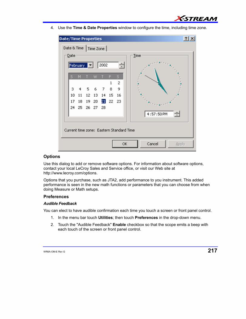
WR6A-OM-E Rev G 217
4. Use the Time & Date Properties window to configure the time, including time zone.
Options Use this dialog to add or remove software options. For information about software options, contact your local LeCroy Sales and Service office, or visit our Web site at http://www.lecroy.com/options.
Options that you purchase, such as JTA2, add performance to you instrument. This added performance is seen in the new math functions or parameters that you can choose from when doing Measure or Math setups.
Preferences Audible Feedback
You can elect to have audible confirmation each time you touch a screen or front panel control.
1. In the menu bar touch Utilities; then touch Preferences in the drop-down menu.
2. Touch the "Audible Feedback" Enable checkbox so that the scope emits a beep with each touch of the screen or front panel control.
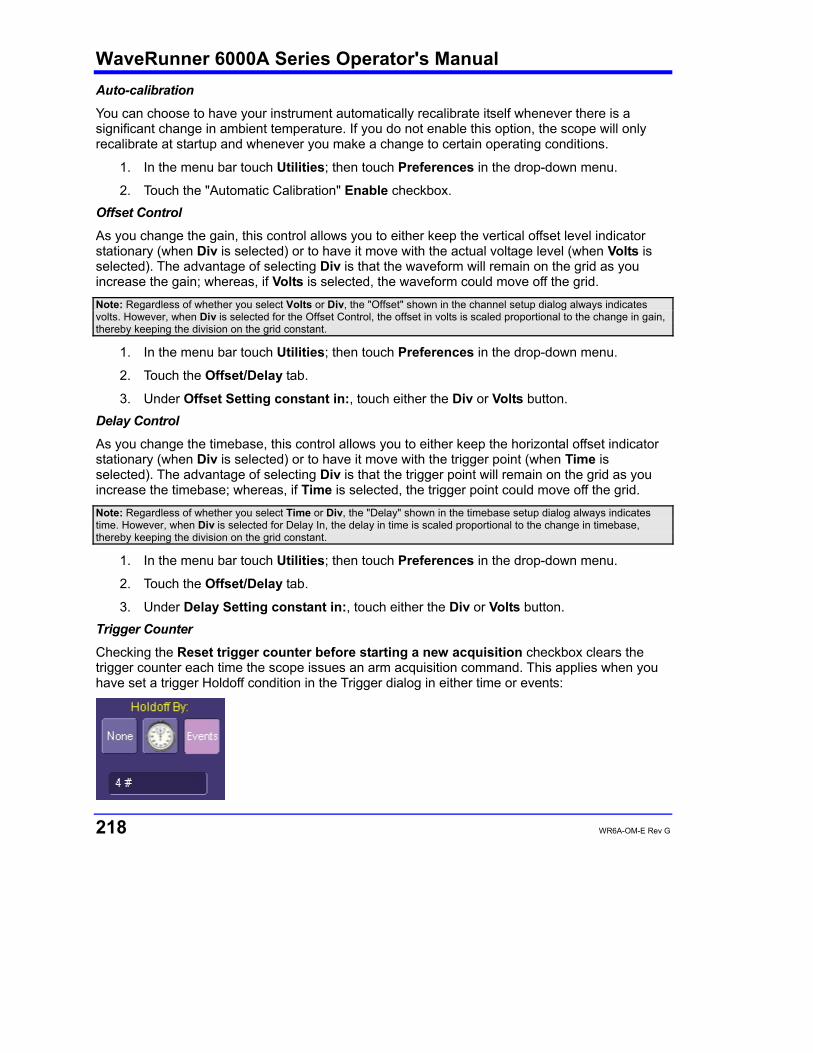
WaveRunner 6000A Series Operator's Manual
218 WR6A-OM-E Rev G
Auto-calibration
You can choose to have your instrument automatically recalibrate itself whenever there is a significant change in ambient temperature. If you do not enable this option, the scope will only recalibrate at startup and whenever you make a change to certain operating conditions.
1. In the menu bar touch Utilities; then touch Preferences in the drop-down menu.
2. Touch the "Automatic Calibration" Enable checkbox. Offset Control
As you change the gain, this control allows you to either keep the vertical offset level indicator stationary (when Div is selected) or to have it move with the actual voltage level (when Volts is selected). The advantage of selecting Div is that the waveform will remain on the grid as you increase the gain; whereas, if Volts is selected, the waveform could move off the grid. Note: Regardless of whether you select Volts or Div, the "Offset" shown in the channel setup dialog always indicates volts. However, when Div is selected for the Offset Control, the offset in volts is scaled proportional to the change in gain, thereby keeping the division on the grid constant.
1. In the menu bar touch Utilities; then touch Preferences in the drop-down menu.
2. Touch the Offset/Delay tab.
3. Under Offset Setting constant in:, touch either the Div or Volts button. Delay Control
As you change the timebase, this control allows you to either keep the horizontal offset indicator stationary (when Div is selected) or to have it move with the trigger point (when Time is selected). The advantage of selecting Div is that the trigger point will remain on the grid as you increase the timebase; whereas, if Time is selected, the trigger point could move off the grid. Note: Regardless of whether you select Time or Div, the "Delay" shown in the timebase setup dialog always indicates time. However, when Div is selected for Delay In, the delay in time is scaled proportional to the change in timebase, thereby keeping the division on the grid constant.
1. In the menu bar touch Utilities; then touch Preferences in the drop-down menu.
2. Touch the Offset/Delay tab.
3. Under Delay Setting constant in:, touch either the Div or Volts button. Trigger Counter
Checking the Reset trigger counter before starting a new acquisition checkbox clears the trigger counter each time the scope issues an arm acquisition command. This applies when you have set a trigger Holdoff condition in the Trigger dialog in either time or events:
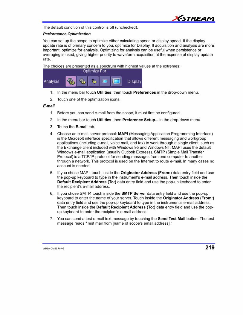
WR6A-OM-E Rev G 219
The default condition of this control is off (unchecked). Performance Optimization
You can set up the scope to optimize either calculating speed or display speed. If the display update rate is of primary concern to you, optimize for Display. If acquisition and analysis are more important, optimize for analysis. Optimizing for analysis can be useful when persistence or averaging is used, giving higher priority to waveform acquisition at the expense of display update rate.
The choices are presented as a spectrum with highest values at the extremes:
1. In the menu bar touch Utilities; then touch Preferences in the drop-down menu.
2. Touch one of the optimization icons. E-mail
1. Before you can send e-mail from the scope, it must first be configured.
2. In the menu bar touch Utilities, then Preference Setup... in the drop-down menu.
3. Touch the E-mail tab.
4. Choose an e-mail server protocol: MAPI (Messaging Application Programming Interface) is the Microsoft interface specification that allows different messaging and workgroup applications (including e-mail, voice mail, and fax) to work through a single client, such as the Exchange client included with Windows 95 and Windows NT. MAPI uses the default Windows e-mail application (usually Outlook Express). SMTP (Simple Mail Transfer Protocol) is a TCP/IP protocol for sending messages from one computer to another through a network. This protocol is used on the Internet to route e-mail. In many cases no account is needed.
5. If you chose MAPI, touch inside the Originator Address (From:) data entry field and use the pop-up keyboard to type in the instrument's e-mail address. Then touch inside the Default Recipient Address (To:) data entry field and use the pop-up keyboard to enter the recipient's e-mail address.
6. If you chose SMTP, touch inside the SMTP Server data entry field and use the pop-up keyboard to enter the name of your server. Touch inside the Originator Address (From:) data entry field and use the pop-up keyboard to type in the instrument's e-mail address. Then touch inside the Default Recipient Address (To:) data entry field and use the pop-up keyboard to enter the recipient's e-mail address.
7. You can send a test e-mail text message by touching the Send Test Mail button. The test message reads "Test mail from [name of scope's email address]."
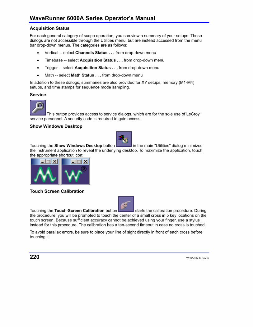
WaveRunner 6000A Series Operator's Manual
220 WR6A-OM-E Rev G
Acquisition Status For each general category of scope operation, you can view a summary of your setups. These dialogs are not accessible through the Utilities menu, but are instead accessed from the menu bar drop-down menus. The categories are as follows:
• Vertical -- select Channels Status . . . from drop-down menu
• Timebase -- select Acquisition Status . . . from drop-down menu
• Trigger -- select Acquisition Status . . . from drop-down menu
• Math -- select Math Status . . . from drop-down menu
In addition to these dialogs, summaries are also provided for XY setups, memory (M1-M4) setups, and time stamps for sequence mode sampling.
Service
This button provides access to service dialogs, which are for the sole use of LeCroy service personnel. A security code is required to gain access.
Show Windows Desktop
Touching the Show Windows Desktop button in the main "Utilities" dialog minimizes the instrument application to reveal the underlying desktop. To maximize the application, touch the appropriate shortcut icon:
.
Touch Screen Calibration
Touching the Touch-Screen Calibration button starts the calibration procedure. During the procedure, you will be prompted to touch the center of a small cross in 5 key locations on the touch screen. Because sufficient accuracy cannot be achieved using your finger, use a stylus instead for this procedure. The calibration has a ten-second timeout in case no cross is touched.
To avoid parallax errors, be sure to place your line of sight directly in front of each cross before touching it.
WR6A-OM-E Rev G 221
CUSTOMIZATION Customizing Your Instrument The instrument provides powerful capability to add your own parameters, functions, display algorithms, or other routines to the scope user interface without having to leave the instrument application environment. You can customize the instrument to your needs by using the power of programs such as Excel™, Mathcad™, and MATLAB™, or by scripting in VBS. Whichever method you use, the results appear on the instrument's display together with the signals that you started with. This ability offers tremendous advantages in solving unique problems for a large range of applications, with comparatively little effort from you. Introduction
Instrument customization provides these important capabilities:
• You can export data to programs, without leaving the instrument environment.
• You can get results back from those programs, and display them on the instrument, without leaving the instrument application environment.
• Once the result is returned, you can perform additional scope operations, such as measuring with cursors, applying parameters, or performing additional functions on the waveform, in exactly the same way as for a normal waveform.
• You can program the scope yourself.
• The instrument does not just provide connectivity with data downloads to other programs. It provides true customizable interaction with these other programs, and allows you to truly customize the scope to do the exact job you want it to do. The advantages to this are many:
• You can use the standard processing power of the instrument to do most of your calculations
• You only need to write the function, parameter, display algorithm, etc. that specifically applies to your need and that the instrument doesn’t contain.
• You can view the final result on the instrument display, and use all of the instrument's tools to understand the result.
• You can do additional processing on the result by applying either standard instrument parameters, functions, etc. to the returned result, or even more powerfully, adding chained customized functions. For example, you can do an Excel calculation on a result with a MATLAB function applied to it.
Solutions
Engineers do not buy equipment; they buy solutions. But what solutions can be reached from a set of instrument waveform data? In principle, anything that can be logically derived from those data, given the limitations of signal-to-noise ratio and processing time. Here are some examples of what can be done with a customized instrument:

WaveRunner 6000A Series Operator's Manual
222 WR6A-OM-E Rev G
• Changing the units of a grid to joules, newtons, amps, etc.
• Creating a new waveform by manipulating the data of one or two input waveforms
• Creating a new waveform without using any of the input data
• Creating a new parameter by manipulating the data of one or two input waveforms
• Changing a vertical scale or a horizontal scale from linear to non-linear
You don’t have to use all the data from the input waveforms: you can select data from one or more segments, which need not be aligned in the two-input waveforms. Examples
Example 1: Simple math functions using VBScript
WaveOut is the waveform being returned to the instrument (F1 in this case). WaveIn is the input waveform (C1 in this case) You can see that the F1 result is displayed on the scope, and can be processed further.
Example 2: Another simple math function using VBScript
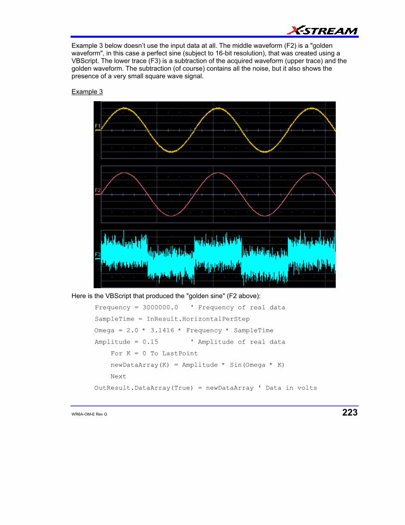
WR6A-OM-E Rev G 223
Example 3 below doesn’t use the input data at all. The middle waveform (F2) is a "golden waveform", in this case a perfect sine (subject to 16-bit resolution), that was created using a VBScript. The lower trace (F3) is a subtraction of the acquired waveform (upper trace) and the golden waveform. The subtraction (of course) contains all the noise, but it also shows the presence of a very small square wave signal.
Example 3
Here is the VBScript that produced the "golden sine" (F2 above):
Frequency = 3000000.0 ' Frequency of real data
SampleTime = InResult.HorizontalPerStep
Omega = 2.0 * 3.1416 * Frequency * SampleTime
Amplitude = 0.15 ' Amplitude of real data
For K = 0 To LastPoint
newDataArray(K) = Amplitude * Sin(Omega * K)
Next
OutResult.DataArray(True) = newDataArray ' Data in volts
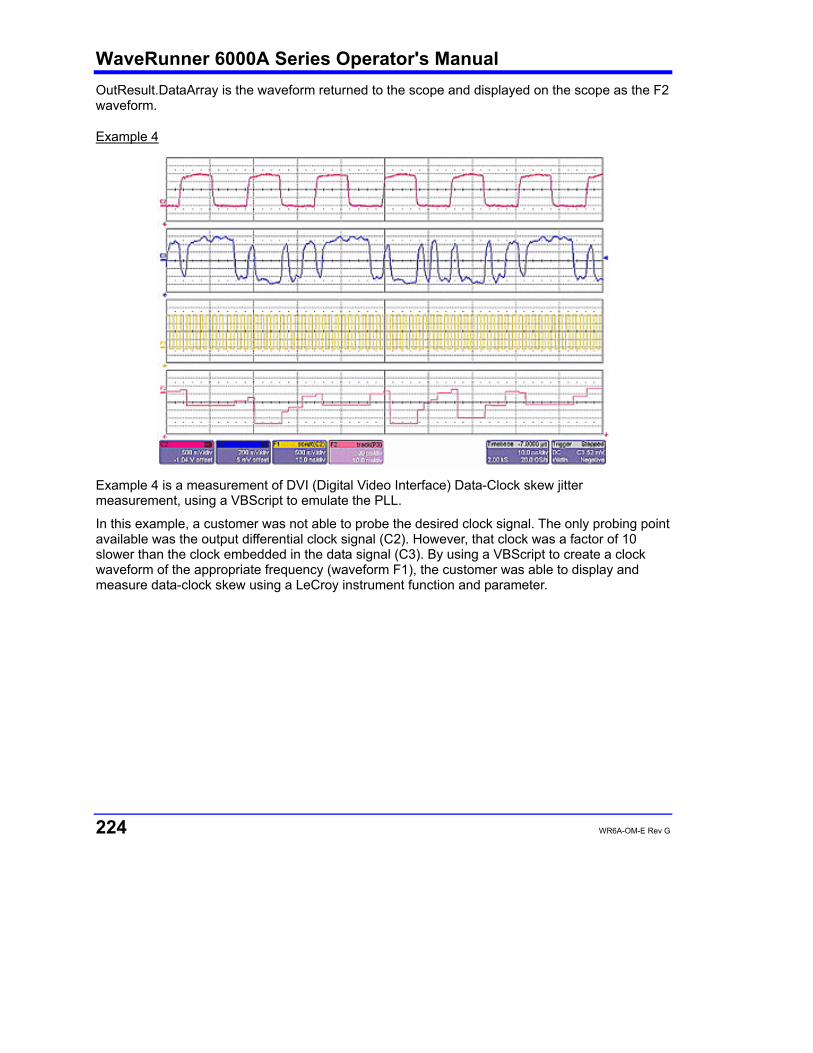
WaveRunner 6000A Series Operator's Manual
224 WR6A-OM-E Rev G
OutResult.DataArray is the waveform returned to the scope and displayed on the scope as the F2 waveform.
Example 4
Example 4 is a measurement of DVI (Digital Video Interface) Data-Clock skew jitter measurement, using a VBScript to emulate the PLL.
In this example, a customer was not able to probe the desired clock signal. The only probing point available was the output differential clock signal (C2). However, that clock was a factor of 10 slower than the clock embedded in the data signal (C3). By using a VBScript to create a clock waveform of the appropriate frequency (waveform F1), the customer was able to display and measure data-clock skew using a LeCroy instrument function and parameter.
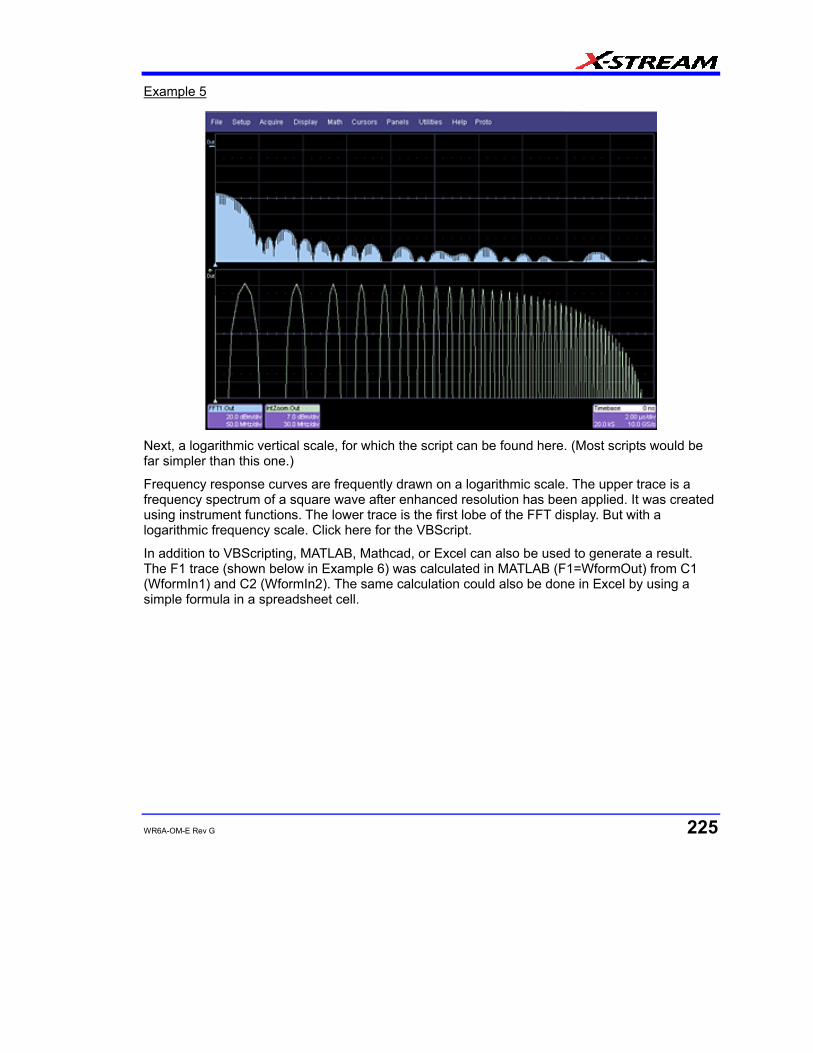
WR6A-OM-E Rev G 225
Example 5
Next, a logarithmic vertical scale, for which the script can be found here. (Most scripts would be far simpler than this one.)
Frequency response curves are frequently drawn on a logarithmic scale. The upper trace is a frequency spectrum of a square wave after enhanced resolution has been applied. It was created using instrument functions. The lower trace is the first lobe of the FFT display. But with a logarithmic frequency scale. Click here for the VBScript.
In addition to VBScripting, MATLAB, Mathcad, or Excel can also be used to generate a result. The F1 trace (shown below in Example 6) was calculated in MATLAB (F1=WformOut) from C1 (WformIn1) and C2 (WformIn2). The same calculation could also be done in Excel by using a simple formula in a spreadsheet cell.
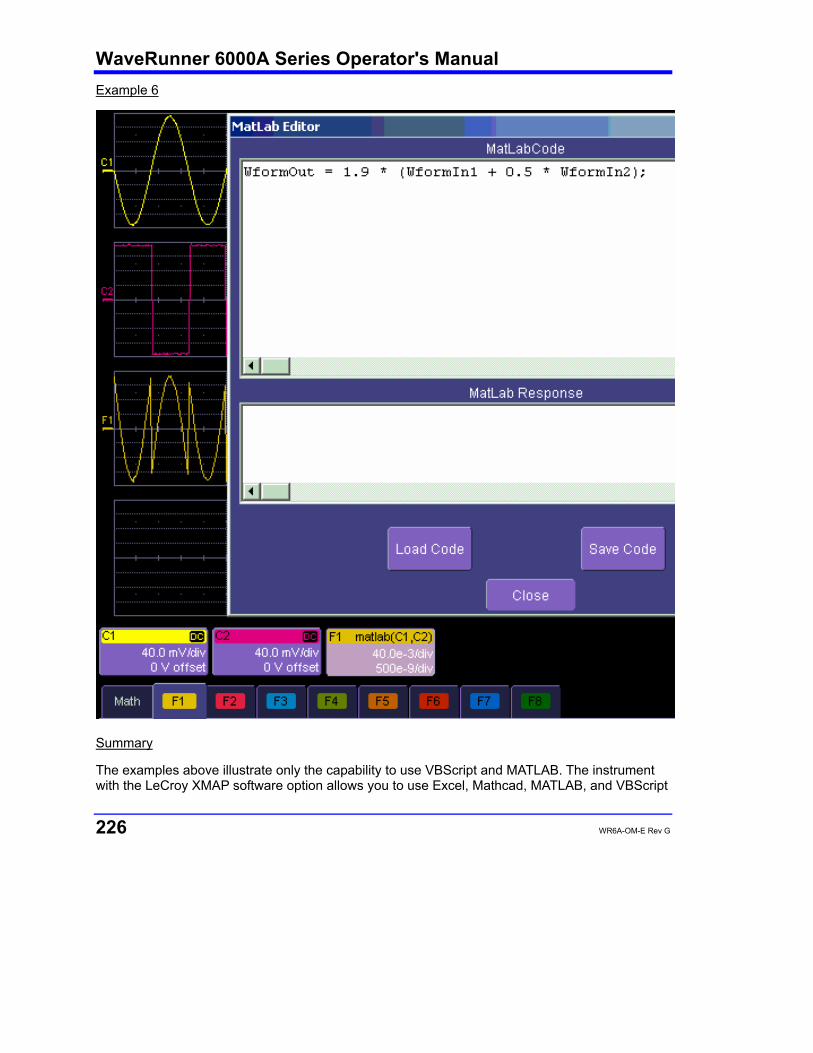
WaveRunner 6000A Series Operator's Manual
226 WR6A-OM-E Rev G
Example 6
Summary
The examples above illustrate only the capability to use VBScript and MATLAB. The instrument with the LeCroy XMAP software option allows you to use Excel, Mathcad, MATLAB, and VBScript

WR6A-OM-E Rev G 227
in this manner. Of course, you will need to load Excel, Mathcad, or MATLAB in the scope (VBScript does not require any additional software) to take advantage of the capability. You can think of these functions as "subroutines" of the instrument's main software, which take in waveform data and other variables like vertical scale and offset, and horizontal scale and offset. These functions then return a waveform or a parameter as required. In addition, you can view the calculated data directly in Excel, MATLAB, or Mathcad, if you desire. What is Excel?
Excel is a program within Microsoft Office. With it you can place data in the cells of a spreadsheet, calculate other values from them, prepare charts of many kinds, use mathematical and statistical functions, and communicate with other programs in Office. From the instrument you can send data to Excel (where processing can take place) and return the results to the instrument. What is Mathcad?
Mathcad is a software package from MathSoft. It provides an integrated environment for performing numerical calculations and solving equations, and communicating with other programs. Results can be presented in tabular or graphical form. What is MATLAB?
MATLAB is a software package from MathWorks that provides an environment for work in computation and mathematics. An interactive language and graphics are provided. What is VBS?
VBS is a programming language, but you don’t write it in a special environment such as C++ or Visual Basic; you write it within your own application. In the instrument, a few clicks or button pushes will get you into an editing panel where you can write what you want. You cannot crash the scope, or in any other way interfere with its workings, because the system is completely protected.
A product of Microsoft and a subset of Visual Basic, VBS can be learned very quickly if you have some experience in any programming language. The VBS processing function can collect a number of useful variables from the scope, including waveform data and useful variables such as volts per division and time per division. The output from a script can be a waveform or a parameter, and you can choose your own values for variables such as volts per division.
The idea of a VBS function is that you start with an input waveform, operate on some or all of the values with a script, and show the result on a scope grid, like any other waveform.
VBScript customization is built into the instrument, so no additional programs need to be loaded to take advantage of this capability.
The following diagrams were made by changing a small part, in some cases just one line, of a standard VBScript. VBS is a well-known standard language, with excellent support documentation, and it is easy to use in several different environments.

WaveRunner 6000A Series Operator's Manual
228 WR6A-OM-E Rev G

WR6A-OM-E Rev G 229
These examples are purely illustrative, but you can easily imagine that with a VBScript you can add value to the scope in a very short time. This gives you an instrument that does exactly what you want, time after time, by using your stored setups and scripts. What can you do with a customized instrument?
If you require a result that can be derived logically from the input waveform, you can do it. Many calculations can be done with remarkably small scripts, but if you have no time for scripting, you can use one of the proprietary packages, such as Excel, MATLAB, or Mathcad, which offer immense processing power.
Scaling and Display
Scripting and programming allow a large variety of opportunities. You may, for example, be using transducers. If so, you can change the units of your waveforms, and write N (newtons), J (joules) and so on, and you can introduce scaling factors. If the transducers are non-linear, you can correct for that, too. You can also transform horizontal scales and vertical scales by manipulating the data. Logarithmic scales in amplitude and frequency are often required. Squaring and taking square roots are needed in certain applications. Here is a picture showing some graphs related to white noise, showing ways of detecting small deviations from the true distribution. The lower two graphs were generated and placed in one trace using a VBScript.
In the next example, four graphs are placed in one trace.
Golden Waveforms
This is a rich field for VBS. An example was given earlier. The only limits to the shapes that can be generated are the vertical resolution and the number of samples.
A practical example – DVI Data-Clock skew
The next example is a measurement of DVI Data-Clock skew jitter measurement, using a VBScript to emulate the PLL. A solution to a practical measurement problem was shown earlier.
WaveRunner 6000A Series Operator's Manual
230 WR6A-OM-E Rev G
These are just a few of the many solutions that can be created.
Calling Excel from Your Instrument Calling Excel Directly from the Instrument
Excel can be directly called from the instrument in two ways:
Using a function F1 through Fx The number of math traces available depends on the software options loaded on your scope. See Specifications.
Excel returns a waveform
Using a parameter P1 through Px The number of parameters available depends on the software options loaded on your scope. See Specifications.
Excel returns a parameter
In both cases, one call to Excel can use two separate waveforms as input. Notes: Excel has a calculation algorithm of 64,000 points (32,000 if you have created a chart in Excel). Therefore, make sure that your acquisition has less than this number of points if you are going to use an Excel calculation. To use this capability, you must have the LeCroy XMAP software option and Excel loaded in your instrument. Select Minimize from the instrument's File menu to access the Excel program directly.
How to Select a Math Function Call The Excel math function is selected from the Math Operator menu, where it appears in the Custom group.
How to Select a Parameter Function Call The Excel Parameter function is selected from the Select Measurement menu, where it appears in the Custom group.
The Excel Control Dialog Once you have invoked an Excel call, you will see a dialog at the right of the screen, allowing you to control the zoom, Excel properties, linking cells, and scale of the output trace from Excel:
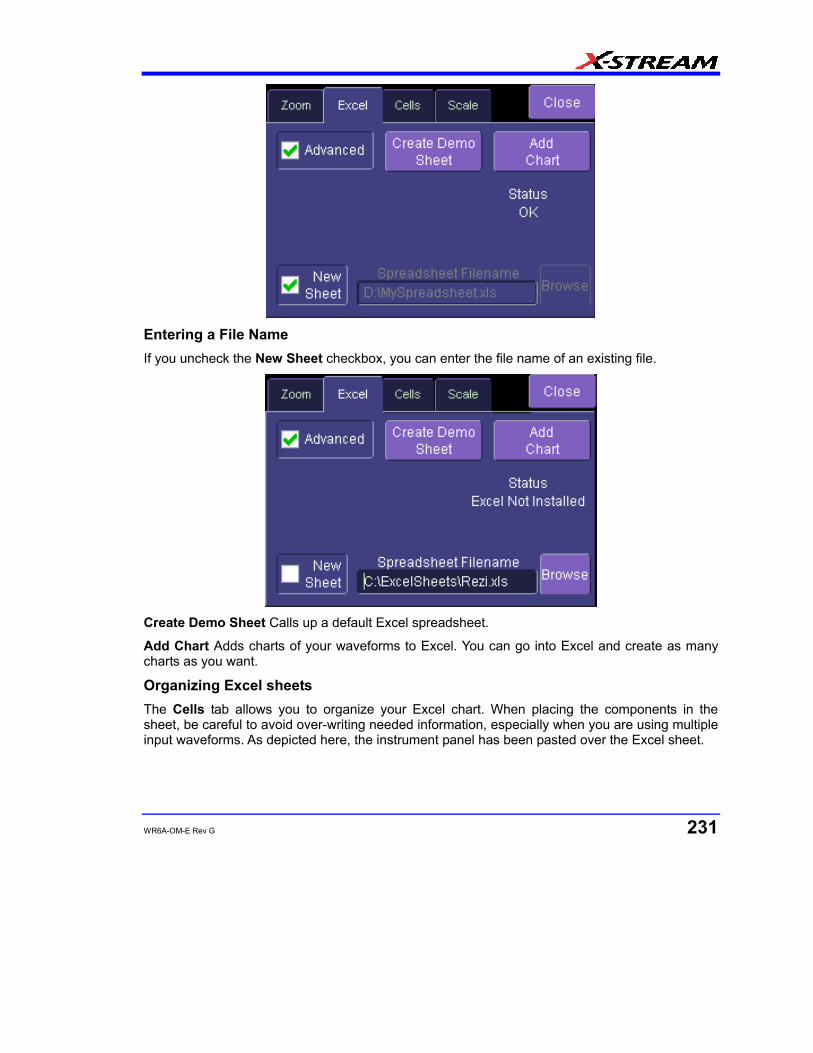
WR6A-OM-E Rev G 231
Entering a File Name If you uncheck the New Sheet checkbox, you can enter the file name of an existing file.
Create Demo Sheet Calls up a default Excel spreadsheet.
Add Chart Adds charts of your waveforms to Excel. You can go into Excel and create as many charts as you want.
Organizing Excel sheets The Cells tab allows you to organize your Excel chart. When placing the components in the sheet, be careful to avoid over-writing needed information, especially when you are using multiple input waveforms. As depicted here, the instrument panel has been pasted over the Excel sheet.

WaveRunner 6000A Series Operator's Manual
232 WR6A-OM-E Rev G
There are three arrays of data for the three waveforms: up to two inputs and one output. There are corresponding small arrays of information about each trace.
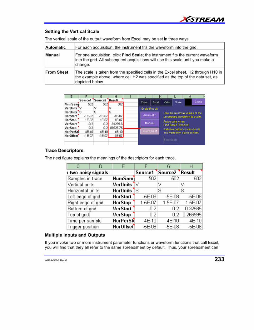
WR6A-OM-E Rev G 233
Setting the Vertical Scale The vertical scale of the output waveform from Excel may be set in three ways:
Automatic For each acquisition, the instrument fits the waveform into the grid.
Manual For one acquisition, click Find Scale; the instrument fits the current waveform into the grid. All subsequent acquisitions will use this scale until you make a change.
From Sheet The scale is taken from the specified cells in the Excel sheet, H2 through H10 in the example above, where cell H2 was specified as the top of the data set, as depicted below.
Trace Descriptors The next figure explains the meanings of the descriptors for each trace.
Multiple Inputs and Outputs If you invoke two or more instrument parameter functions or waveform functions that call Excel, you will find that they all refer to the same spreadsheet by default. Thus, your spreadsheet can
WaveRunner 6000A Series Operator's Manual
234 WR6A-OM-E Rev G
use the data from several waveforms, and you can derive many different combinations of output parameters and waveforms, including some of each, from your spreadsheet. You only have to be careful about the positioning of your cell ranges within the sheet so that no conflicts occur.
Because filling cells in the spreadsheet is a relatively slow process, all unwanted sources (inputs) should be left disabled (unchecked). For example, if you want one waveform and two parameters derived from the data of three waveforms, you can have one function with both sources enabled, one with one source enabled, and one with no sources enabled. The alternative is to use one input in each function.
Examples Simple Excel Example 1
In this example we use Excel to invert or negate a waveform. The first figure shows a part of the screen. The upper trace is the original signal. The lower is the result from Excel.
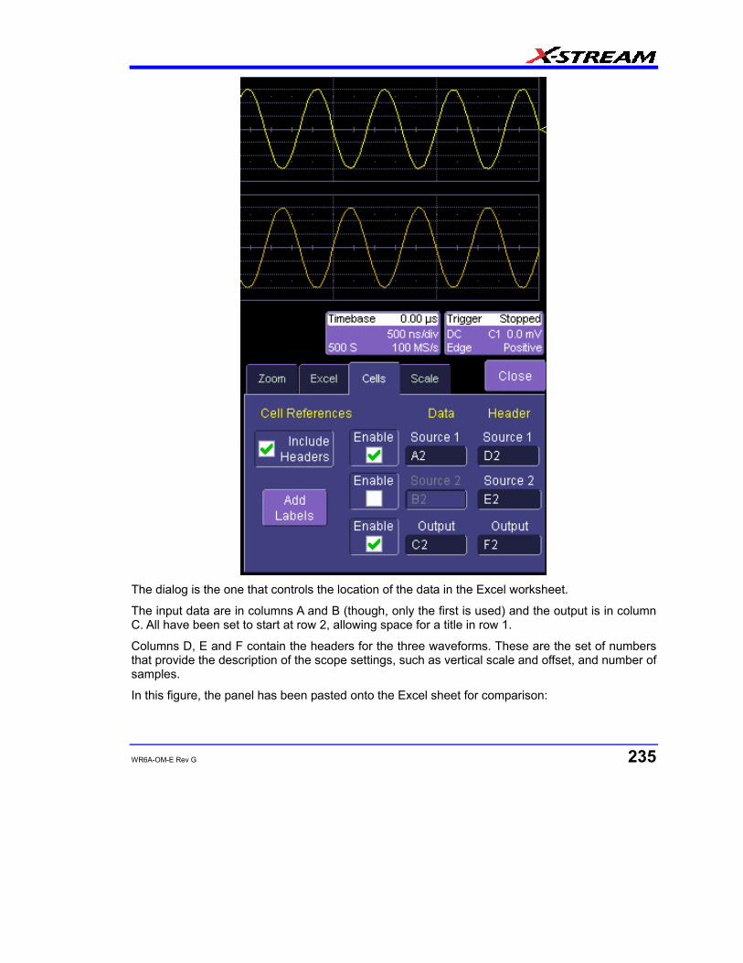
WR6A-OM-E Rev G 235
The dialog is the one that controls the location of the data in the Excel worksheet.
The input data are in columns A and B (though, only the first is used) and the output is in column C. All have been set to start at row 2, allowing space for a title in row 1.
Columns D, E and F contain the headers for the three waveforms. These are the set of numbers that provide the description of the scope settings, such as vertical scale and offset, and number of samples.
In this figure, the panel has been pasted onto the Excel sheet for comparison:
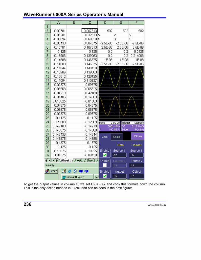
WaveRunner 6000A Series Operator's Manual
236 WR6A-OM-E Rev G
To get the output values in column C, we set C2 = - A2 and copy this formula down the column. This is the only action needed in Excel, and can be seen in the next figure:
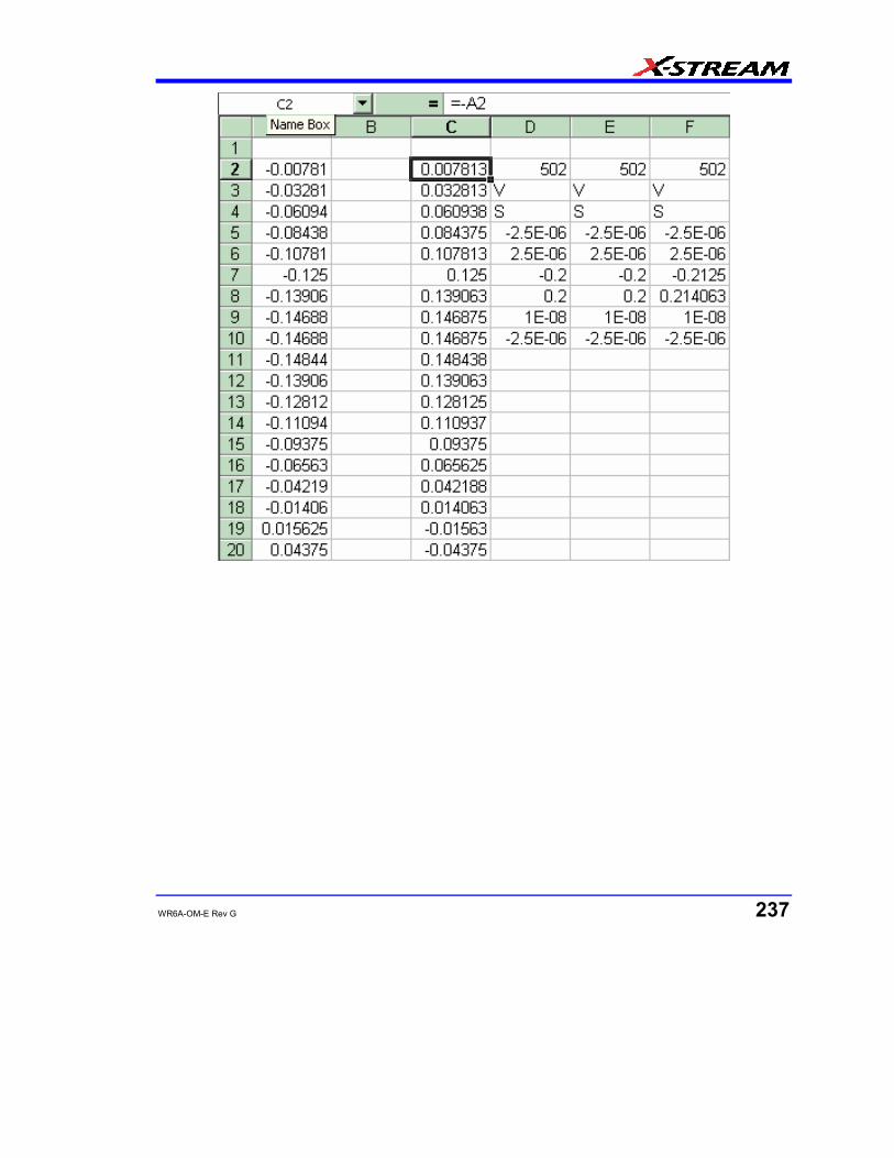
WR6A-OM-E Rev G 237
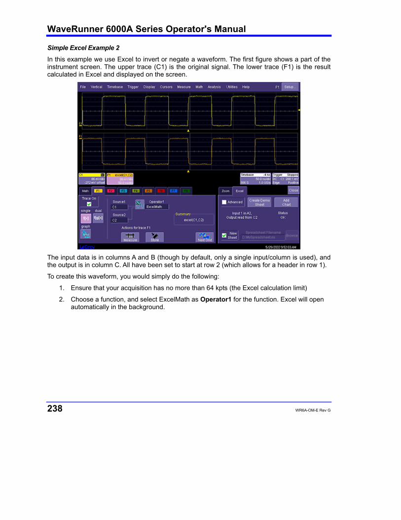
WaveRunner 6000A Series Operator's Manual
238 WR6A-OM-E Rev G
Simple Excel Example 2
In this example we use Excel to invert or negate a waveform. The first figure shows a part of the instrument screen. The upper trace (C1) is the original signal. The lower trace (F1) is the result calculated in Excel and displayed on the screen.
The input data is in columns A and B (though by default, only a single input/column is used), and the output is in column C. All have been set to start at row 2 (which allows for a header in row 1).
To create this waveform, you would simply do the following:
1. Ensure that your acquisition has no more than 64 kpts (the Excel calculation limit)
2. Choose a function, and select ExcelMath as Operator1 for the function. Excel will open automatically in the background.
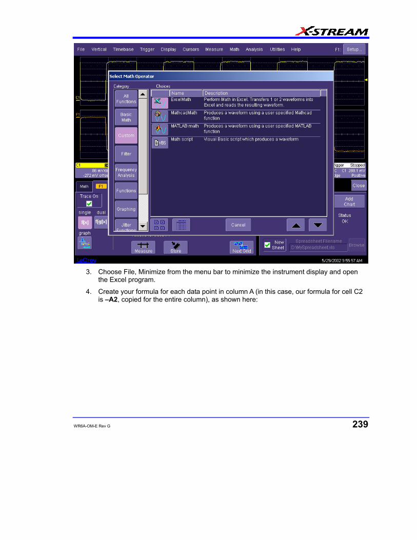
WR6A-OM-E Rev G 239
3. Choose File, Minimize from the menu bar to minimize the instrument display and open
the Excel program.
4. Create your formula for each data point in column A (in this case, our formula for cell C2 is –A2, copied for the entire column), as shown here:

WaveRunner 6000A Series Operator's Manual
240 WR6A-OM-E Rev G
.
5. Retrigger the scope (if it is not currently triggering)
6. Return to the program
Note that the only action that was needed in Excel was to create the formula in column C for each data point in column A. The instrument automatically opens Excel, puts the waveform data in the correct columns, and returns the calculated data back to the display as the chosen F trace. This Excel-calculated trace can have further measurements or math calculations performed on it, if desired.
You can also create a chart of the data in Excel automatically and view the data there. Simply press the Add Chart button in the instrument's Excel dialog and a chart of the input (top chart) and Excel calculated output (bottom chart) will be automatically created in the spreadsheet. The chart will be updated automatically as the scope is triggered.
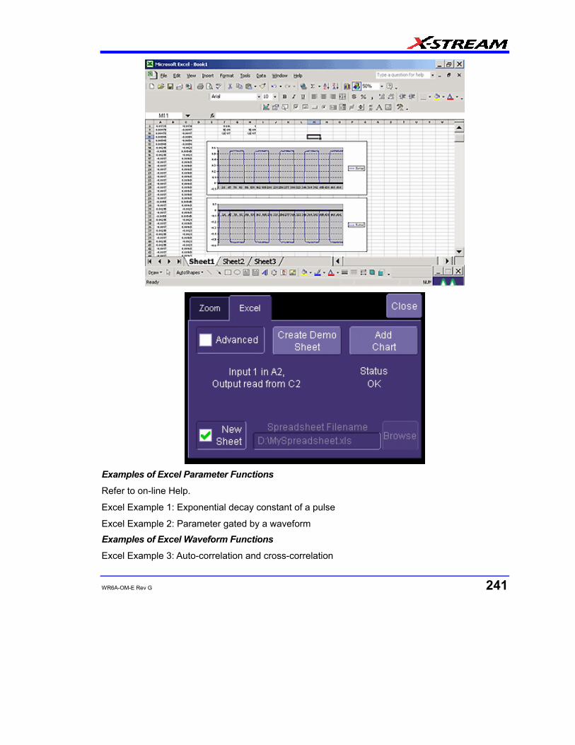
WR6A-OM-E Rev G 241
Examples of Excel Parameter Functions
Refer to on-line Help.
Excel Example 1: Exponential decay constant of a pulse
Excel Example 2: Parameter gated by a waveform Examples of Excel Waveform Functions
Excel Example 3: Auto-correlation and cross-correlation
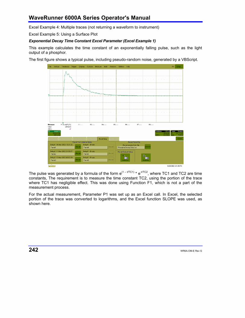
WaveRunner 6000A Series Operator's Manual
242 WR6A-OM-E Rev G
Excel Example 4: Multiple traces (not returning a waveform to instrument)
Excel Example 5: Using a Surface Plot Exponential Decay Time Constant Excel Parameter (Excel Example 1)
This example calculates the time constant of an exponentially falling pulse, such as the light output of a phosphor.
The first figure shows a typical pulse, including pseudo-random noise, generated by a VBScript.
The pulse was generated by a formula of the form e(1 – t/TC1) * e-t/TC2, where TC1 and TC2 are time constants, The requirement is to measure the time constant TC2, using the portion of the trace where TC1 has negligible effect. This was done using Function F1, which is not a part of the measurement process.
For the actual measurement, Parameter P1 was set up as an Excel call. In Excel, the selected portion of the trace was converted to logarithms, and the Excel function SLOPE was used, as shown here.
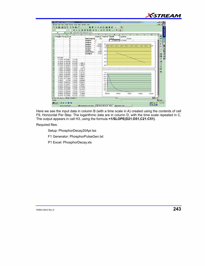
WR6A-OM-E Rev G 243
Here we see the input data in column B (with a time scale in A) created using the contents of cell F9, Horizontal Per Step. The logarithmic data are in column D, with the time scale repeated in C. The output appears in cell H3, using the formula =1/SLOPE(D21:D51,C21:C51).
Required files:
Setup: PhosphorDecay20Apr.lss
F1 Generator: PhosphorPulseGen.txt
P1 Excel: PhosphorDecay.xls
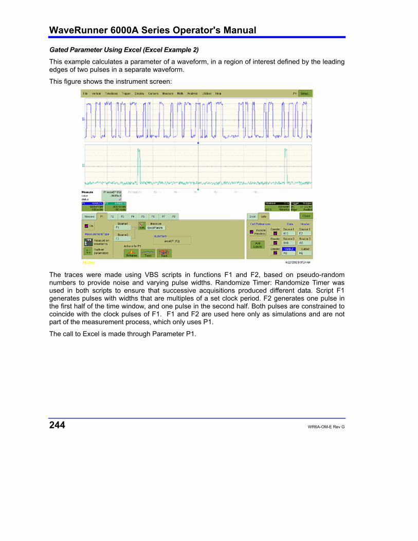
WaveRunner 6000A Series Operator's Manual
244 WR6A-OM-E Rev G
Gated Parameter Using Excel (Excel Example 2)
This example calculates a parameter of a waveform, in a region of interest defined by the leading edges of two pulses in a separate waveform.
This figure shows the instrument screen:
The traces were made using VBS scripts in functions F1 and F2, based on pseudo-random numbers to provide noise and varying pulse widths. Randomize Timer: Randomize Timer was used in both scripts to ensure that successive acquisitions produced different data. Script F1 generates pulses with widths that are multiples of a set clock period. F2 generates one pulse in the first half of the time window, and one pulse in the second half. Both pulses are constrained to coincide with the clock pulses of F1. F1 and F2 are used here only as simulations and are not part of the measurement process, which only uses P1.
The call to Excel is made through Parameter P1.

WR6A-OM-E Rev G 245
The next figure shows a part of the Excel workbook.
Here we see the gated waveform that has been created in Excel. The Mean parameter during the region of interest (ROI) is placed in cell H3.
How Does this Work?
The amplitude of the signal is about 0.3 volts, and the screen height is 0.4 volts, as derived from cells F7 and Fx. A threshold value for amplitude was calculated by placing 0.5 * (Fy – Fx) in cell A4.
Remember that in the instrument the sources were defined to be A10 and B10. This means that the first point on the waveform will be read into A10, and, since the waveform has 500 points, the last point will be read into A510. The same holds true for F2 and column B, since F2 is assigned as Source2, and data is defined to write into column B starting with cell B10.
To create the gating function in column C, the cell C10 was given the following formula:
IF ( ( B10 – B9) > $A$4, 1 – C9, C9). This was copied down the column. Column D, the output column, is simply A * C.
The output was defined as cell H3.
The required mean in cell H3 is given by SUM (D10 : D509) / SUM (C10 : C509), for a 500 point waveform.
Required files:

WaveRunner 6000A Series Operator's Manual
246 WR6A-OM-E Rev G
Setup: GatedParameterExcel.lss
Function F1: RandomPulses22Apr.txt
Function F2: RandomGate22Apr.txt
Parameter P1: GatedMean.xls Correlation Excel Waveform Function (Excel Example 3)
This example uses an Excel waveform function to examine the cross-correlation between two signals, which are both noisy sinusoidal segments. The correlation trace is, of necessity, shorter than the input traces.
The noise was generated using pseudo-random numbers. Randomize Timer was included in the VBScript to ensure that the two traces differed, and that subsequent acquisitions differed. Functions F1 and F2 are included only to simulate signals, and are not part of the measurement process, which is performed by F3.
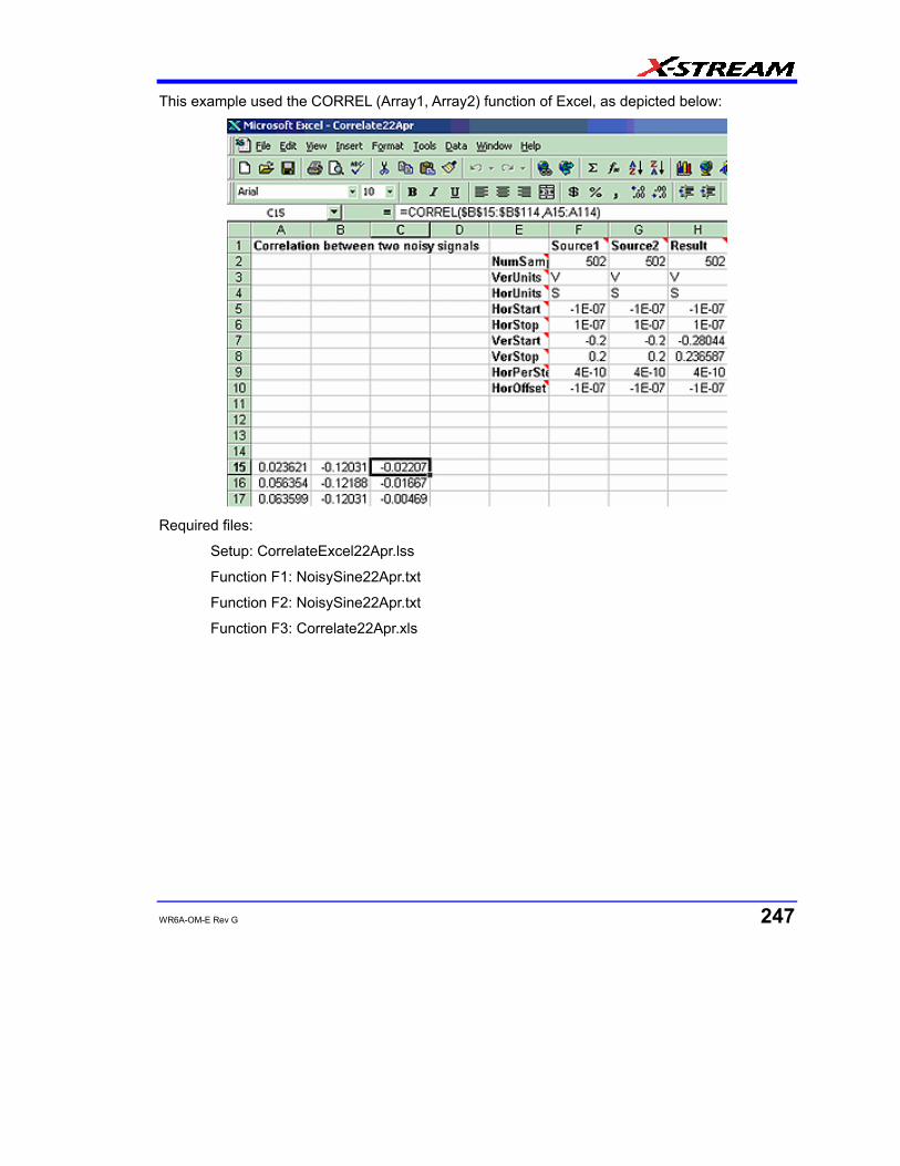
WR6A-OM-E Rev G 247
This example used the CORREL (Array1, Array2) function of Excel, as depicted below:
Required files:
Setup: CorrelateExcel22Apr.lss
Function F1: NoisySine22Apr.txt
Function F2: NoisySine22Apr.txt
Function F3: Correlate22Apr.xls

WaveRunner 6000A Series Operator's Manual
248 WR6A-OM-E Rev G
Multiple Traces on One Grid (Excel Example 4)
This example shows how you can place multiple traces in one picture, with only two operations in an Excel sheet. Depicted below is an example from an Excel spreadsheet.
Here is an original instrument trace.
The method is very simple. First, the waveform is transferred to an Excel spreadsheet by means of an instrument Excel call. Second, two operations are needed in Excel: placing a simple formula in one cell, and copying that formula into a range of cells.

WR6A-OM-E Rev G 249
Depicted below is the required Excel formula.
In fact, the simple expression B374 + 0.02 comprises several components. The original instrument trace is in column B, and the plot is required to start at cell B134. The traces repeat at intervals of 250 cells. Let us call this interval R. If we require a horizontal displacement D, then in cell CN we write B(N + R – D). In this example D is 10. Finally we may want a vertical displacement V, and we write B(N + R – D) + V. In this example, V is 0.02. D and V can be zero if required, as depicted below. All that remains is to copy the formula to the required range of cells.
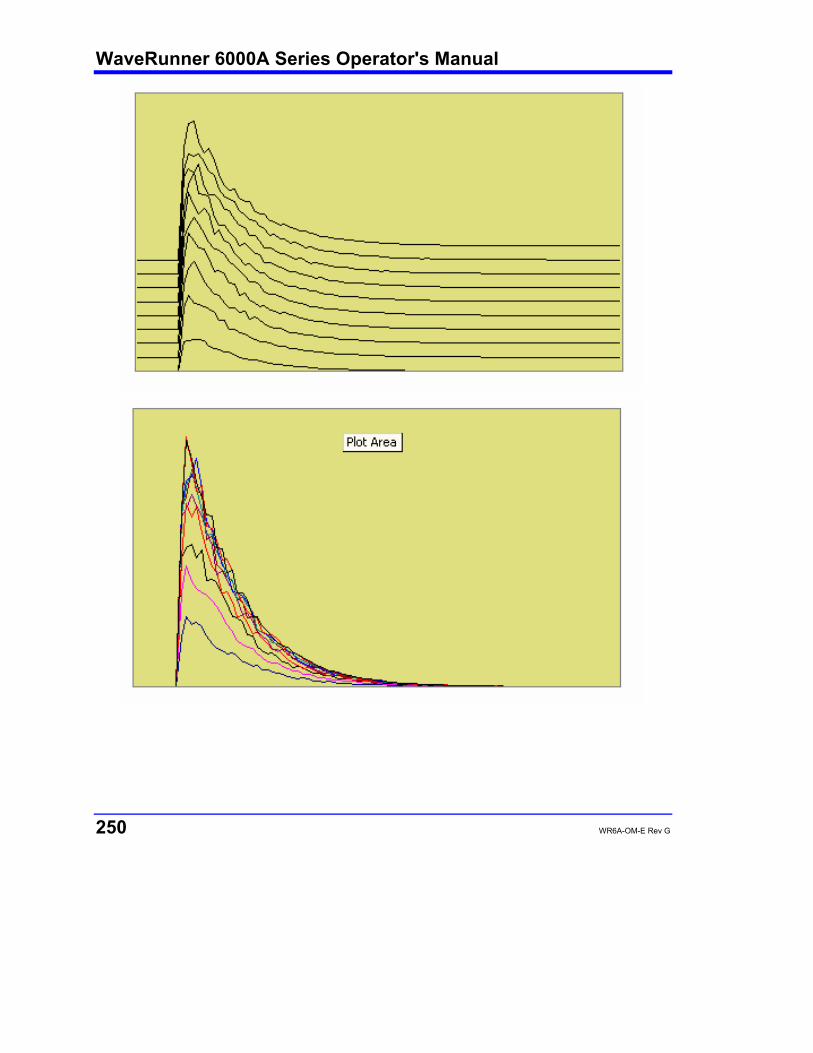
WaveRunner 6000A Series Operator's Manual
250 WR6A-OM-E Rev G
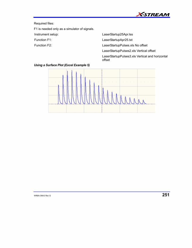
WR6A-OM-E Rev G 251
Required files:
F1 is needed only as a simulator of signals.
Instrument setup: LaserStartup25Apr.lss
Function F1: LaserStartupApr25.txt
Function F2: LaserStartupPulses.xls No offset
LaserStartupPulses2.xls Vertical offset
LaserStartupPulses3.xls Vertical and horizontal offset
Using a Surface Plot (Excel Example 5)
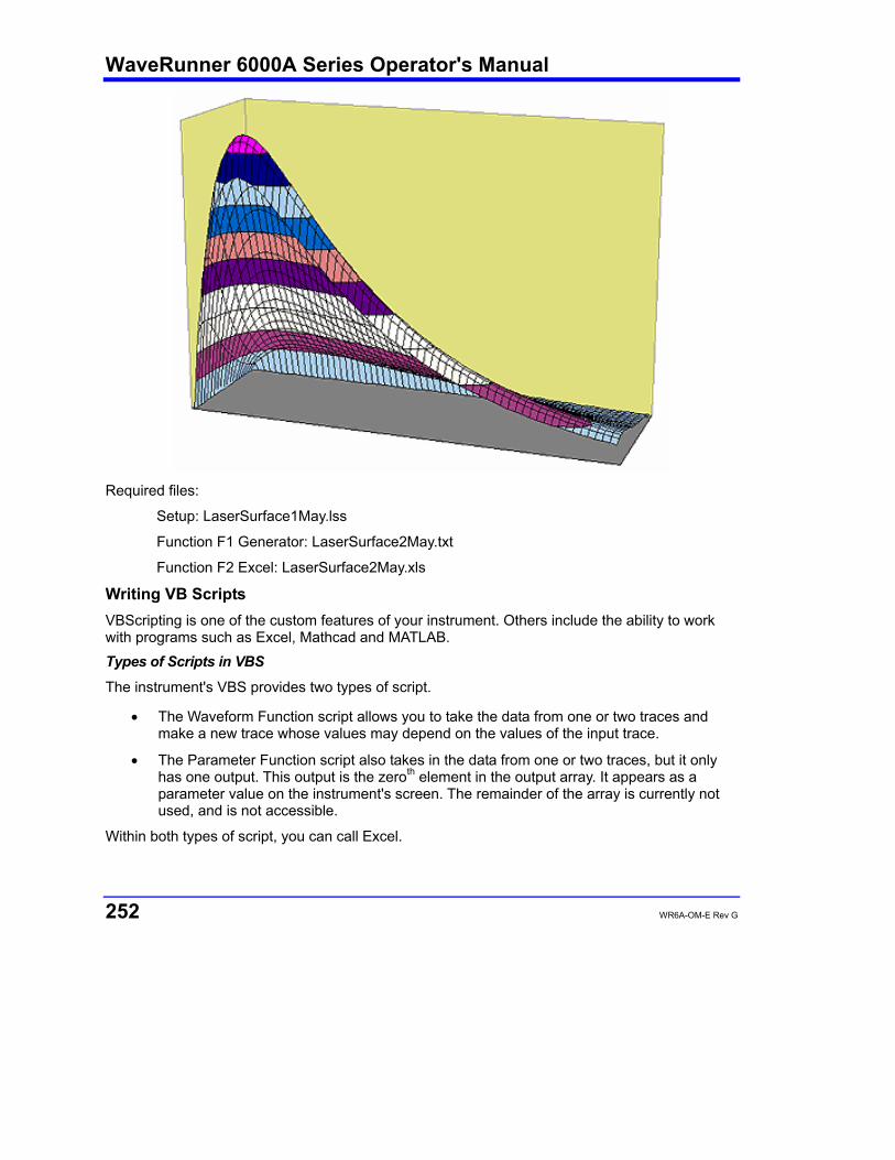
WaveRunner 6000A Series Operator's Manual
252 WR6A-OM-E Rev G
Required files:
Setup: LaserSurface1May.lss
Function F1 Generator: LaserSurface2May.txt
Function F2 Excel: LaserSurface2May.xls
Writing VB Scripts VBScripting is one of the custom features of your instrument. Others include the ability to work with programs such as Excel, Mathcad and MATLAB. Types of Scripts in VBS
The instrument's VBS provides two types of script.
• The Waveform Function script allows you to take the data from one or two traces and make a new trace whose values may depend on the values of the input trace.
• The Parameter Function script also takes in the data from one or two traces, but it only has one output. This output is the zeroth element in the output array. It appears as a parameter value on the instrument's screen. The remainder of the array is currently not used, and is not accessible.
Within both types of script, you can call Excel.

WR6A-OM-E Rev G 253
Loading and Saving VBScripts
From the editing panel you can save your script and you can load a previous one. Should you forget to save a script, please note that when you save your setup, it has your current scripts embedded in it. Therefore it is a good idea to save your setup frequently. It is worth saving the script separately as well, because it is saved in a suitable format for printing or off-line editing with Notepad. Note that in both these examples the input data are referred to as InResult.DataArray. You can also write InResult1.DataArray and InResult2.DataArray, which refer to the two input traces. InResult.DataArray always refers to input trace 1. These remarks hold for any script that you write.
Example Waveform Function Script: Square of a waveform
' Example script to produce a waveform
This example calculates the square of
the input waveform.
OutResult.Samples = InResult.Samples ' Visible trace length + 1
' Note that a trace of nominal length 1000 comprises data numbered from
' 0 to 1001. The 1001st point is not visible, so you
' normally use points 0 to 1000,
' giving 1001 points and 1000 intervals between points.
startData = 0
endData = OutResult.Samples
LastPoint = endData - 1 ' because the last point is invisible.
ReDim newArray(OutResult.Samples) ' to store the results
unscaledData = InResult.DataArray(False)
' InResult.DataArray(False) provides
' integer data from -32768 to 32767.
' InResult.DataArray(True) provides real data
' in the same physical unit as the vertical scale of the input trace.
ScaleFactor = 1.0 / 32768 ' to make the trace fill the screen.
For i = 0 To LastPoint
newArray(i) = ScaleFactor * (unscaledData(i)) ^ 2
Next
OutResult.DataArray(False) = newArray ' signed long integer data output
WaveRunner 6000A Series Operator's Manual
254 WR6A-OM-E Rev G
Example Parameter Function Script: RMS of a waveform
' Example script to produce a parameter.
' This script calculates the root mean square
' of the input waveform.
' Note that a trace of nominal length 1000 has data from
' 0 to 1001. The 1001st point is not visible, so you
' normally use points 0 to 1000,
' giving 1001 points and 1000 intervals between points.
startData = 0
endData = InResult.Samples
LastPoint = endData - 1 ' because the last point is invisible.
ReDim newArray(InResult.Samples) ' to store the results
unscaledData = InResult.DataArray(True)
' InResult.DataArray(False) provides
' integer data from -32768 to 32767.
' InResult.DataArray(True) provides real data
' in the same unit as the vertical scale of the trace.
Total = 0
For i = 0 To LastPoint
Total = Total + (unscaledData(i)) ^ 2
Next
NewArray(0) = Sqr (Total / (LastPoint + 1)) Place the result in the zeroth element.
OutResult.ValueArray(True) = newArray ' integer data output
The default waveform function script: explanatory notes
InResult.Samples is the number of points in the incoming waveform.
InResult.DataArray(Boolean) (or InResult1.DataArray or InResult2.DataArray) is the array of input data. If the Boolean is True you get scaled real data in the units of the trace. If the Boolean is false you get unscaled integer data in the range -32768 to + 32767.
The value of InResult.Samples is the total number of data in a trace. It is two more than the nominal value given on the screen. The first point DataArray(0), coincides with the left edge of the screen, apart from the wobble caused by the trigger-to-sample clock difference. If the trace length is nominally 500, the right edge of the screen coincides with DataArray(500), which is the 501st
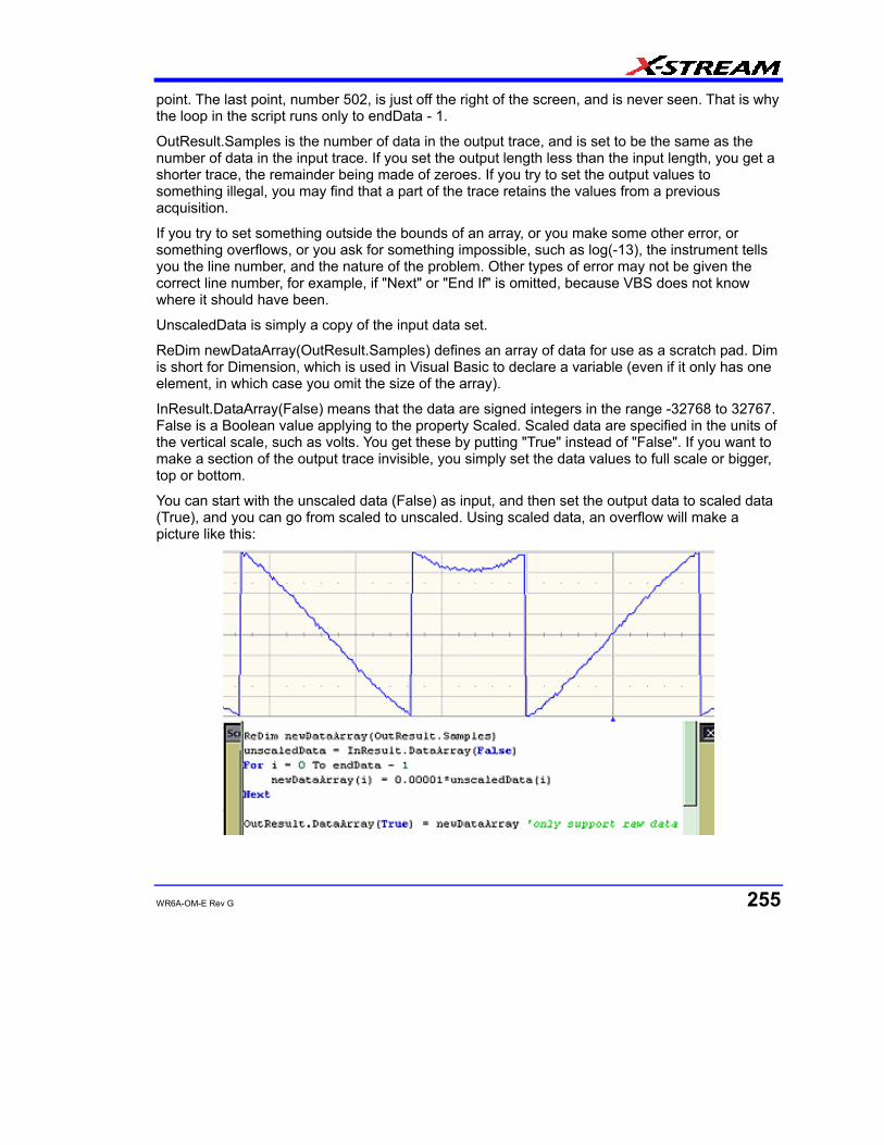
WR6A-OM-E Rev G 255
point. The last point, number 502, is just off the right of the screen, and is never seen. That is why the loop in the script runs only to endData - 1.
OutResult.Samples is the number of data in the output trace, and is set to be the same as the number of data in the input trace. If you set the output length less than the input length, you get a shorter trace, the remainder being made of zeroes. If you try to set the output values to something illegal, you may find that a part of the trace retains the values from a previous acquisition.
If you try to set something outside the bounds of an array, or you make some other error, or something overflows, or you ask for something impossible, such as log(-13), the instrument tells you the line number, and the nature of the problem. Other types of error may not be given the correct line number, for example, if "Next" or "End If" is omitted, because VBS does not know where it should have been.
UnscaledData is simply a copy of the input data set.
ReDim newDataArray(OutResult.Samples) defines an array of data for use as a scratch pad. Dim is short for Dimension, which is used in Visual Basic to declare a variable (even if it only has one element, in which case you omit the size of the array).
InResult.DataArray(False) means that the data are signed integers in the range -32768 to 32767. False is a Boolean value applying to the property Scaled. Scaled data are specified in the units of the vertical scale, such as volts. You get these by putting "True" instead of "False". If you want to make a section of the output trace invisible, you simply set the data values to full scale or bigger, top or bottom.
You can start with the unscaled data (False) as input, and then set the output data to scaled data (True), and you can go from scaled to unscaled. Using scaled data, an overflow will make a picture like this:

WaveRunner 6000A Series Operator's Manual
256 WR6A-OM-E Rev G
You can also start with True and convert to False, but in this case overflows will cause an error message.
Anything after a single quotation mark on a line will not be used by the instrument. This feature is intended for comments, for example
' This is a comment.
A = Amp * Sin(Omega * T) Calculate the output.
InResult.DataArray and OutResult.DataArray are only to be used as shown in the default scripts and in the example scripts: you cannot refer directly to individual elements of these arrays. You have to use your own arrays, in this example, unscaledData and newDataArray. You are not allowed to write statements like the following:
Y = InResult.DataArray (17)
OutResult.DataArray (257) = Z
Some parts of the default script must not be changed because they are a part of the interface. These are highlighted in the following script .
' TODO add your custom code here accessing OutResult and InResult objects
' Here's a small example that just inverts the waveform.
OutResult.Samples = InResult.Samples
startData = 0
endData = OutResult.Samples
newNumPoints = endData - startData
ReDim newDataArray (OutResult.Samples)
unscaledData = InResult.DataArray (False)
For i = 0 To endData - 1
newDataArray (i) = - unscaledData (i)
Next
OutResult.DataArray (False) = newDataArray _' only support raw data
The four highlighted quantities are parts of the interface. The names must be retained. Furthermore, InResult.Samples and InResult.DataArray are inputs, and their values cannot be changed. OutResult.Samples and OutResult.DataArray are outputs, and can be changed, but not directly through their individual elements. The default parameter function script: explanatory notes
The default parameter script is similar to the default waveform script, but there are subtle differences.
WR6A-OM-E Rev G 257
First, the size of the data array is the same as the nominal value: you cannot use or see the extra two points. So "500 points" means just that: 500 points.
Second, the output looks like an array, but only element zero is currently used. You must copy your parameter result into newValueArray(0). As with the arrays of the Waveform Script, you cannot refer directly to elements of the input and output arrays. You may not write something like
OutResult.ValueArray (0) = P.
Note that the unit of the parameter is displayed as the same as the vertical unit of the trace, even if you have squared the data, for example, unless you change the unit yourself.
To find out how to edit a parameter script, click here.
The default parameter script is shown below.
' TODO add your custom code here accessing OutResult and InResult objects
' Here's a small example that just inverts the waveform
numParam = InResult.Samples
ReDim newValueArray(numParam)
scaledData = InResult.DataArray
For i = 0 To numParam-1
newValueArray(i) = -scaledData(i)_' Change this to do something useful.
Next
OutResult.ValueArray = newValueArray 'only support raw data
Your parameter script should include something like this:
A. Do calculation to obtain your parameter value from the input data array.
B. newValueDataArray (0) = ParameterValue
C. OutResult.ValueArray = newValueArray
You can test this script using setup MeanDemoScriptApr2.lss.
You can edit scripts using Notepad, but you will not get any notification of errors.
You are not allowed to write OutResult.ValueArray(0) = MeanParameter.
InResult.DataArray and OutResult.DataArray are only to be used as shown in the default scripts and in the example scripts. You cannot refer to, or modify, any individual element in these arrays. Scripting with VBScript
Separators
The two separators in VBS are the colon : and the single quotation mark .
WaveRunner 6000A Series Operator's Manual
258 WR6A-OM-E Rev G
Using the colon, you can place two or more statements on a line, for example: XMin = 0.0 : XMax = 800.0 : YMin = 0.0 : YMax = 600.0
There is also an implied separator whenever a new line is begun.
Using the quotation mark you can signify that the remainder of the line is a comment: non-executable material that is usually used to clarify the workings of the script. For example:
RMSMax = 32767 / Sqr (2) ' RMS of the largest sinusoid that can be
' fitted into the screen in unscaled mode.
To continue a comment on to another line, another quotation mark is required on the new line. Variable Types
VBS supports the following variable types:
Integer signed 16 bit value in the range -32768 to 32767
Long signed 32 bit value in the range -231 to +231 - 1
Single real number or floating point number
Double real number or floating point number
Boolean Boolean or logical value
String string of characters
When making comparisons using real numbers, beware of testing for equality, because of rounding errors. It may be better to apply a tolerance band. For Boolean, integers and strings, equality is valid.
You can use variables in VBS without declaring the type. The context may force an implicit type assignment. For example, if the result of a calculation is of a different type from the defined type, the type may be changed. Always set out calculations in such a way that type changes will not affect the final result in an undesirable or unpredictable way. If you want to change the type of a variable or a result, use a conversion function that will show others what you intend to happen. The conversion functions are CDbl, CInt, CLng, CSng, CStr.
Variable Names Upper and lower case have no significance in VBS, either in variable names or in keywords (the names reserved by the system), but it is a good idea to be consistent about the spelling of a variable name to avoid confusion. At least 36 characters may be used in a variable name. These can include any combination of alphabetic and numeric characters, and the underscore character. No other punctuation character may be used in a variable name.
Do not use any of the following characters in a variable name:
! @ & $ # ? , * . { } ( ) [ ] = + - ^ % / ~ < > : ;
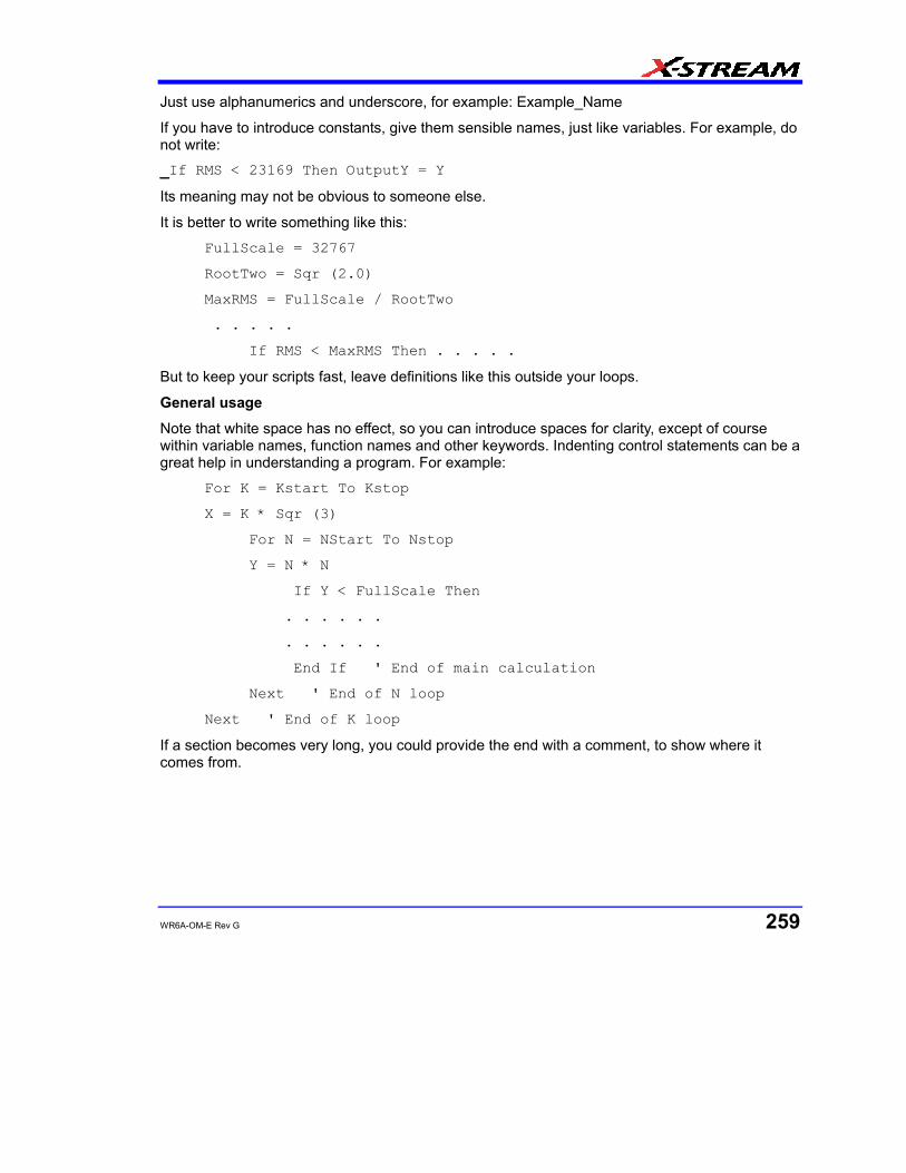
WR6A-OM-E Rev G 259
Just use alphanumerics and underscore, for example: Example_Name
If you have to introduce constants, give them sensible names, just like variables. For example, do not write: _If RMS < 23169 Then OutputY = Y
Its meaning may not be obvious to someone else.
It is better to write something like this:
FullScale = 32767
RootTwo = Sqr (2.0)
MaxRMS = FullScale / RootTwo
. . . . .
If RMS < MaxRMS Then . . . . .
But to keep your scripts fast, leave definitions like this outside your loops.
General usage
Note that white space has no effect, so you can introduce spaces for clarity, except of course within variable names, function names and other keywords. Indenting control statements can be a great help in understanding a program. For example:
For K = Kstart To Kstop
X = K * Sqr (3)
For N = NStart To Nstop
Y = N * N
If Y < FullScale Then
. . . . . .
. . . . . .
End If ' End of main calculation
Next ' End of N loop
Next ' End of K loop
If a section becomes very long, you could provide the end with a comment, to show where it comes from.

WaveRunner 6000A Series Operator's Manual
260 WR6A-OM-E Rev G
Arithmetic Operators As with most other languages, the arithmetic operators are used as follows:
^ Exponentiation A ^ B = A B = A raised to the power B
/ Division A / B = A divided by B
\ Integer division A \ B = A divided by B, truncated to next integer below
* Multiplication A * B = A multiplied by B
+ Addition A + B = B added to A
- Subtraction A B = B subtracted from A
Notes: If there is any possibility that you will be taking the exponent of a negative number, make sure to trap any possible errors arising from such operations as trying to take the square root of a negative number. Logs of negative numbers are forbidden also. If there is any possibility that you will be dividing by zero, make sure to trap this. There are two ways of dealing with these types of problem. One is to prevent it happening by making suitable tests before the calculation is performed. The other is to let it happen, and use an error handling routine. This will be discussed later. Normally in VBScript you will know the range of the data, since all the incoming data are, by definition, integer (unscaled data) or real (scaled data), and they must fit into the screen of the instrument.
Results of Calculations
Sometimes you may see a statement like this:
A = A * A * (Cos (A) + Sin (A) )
The program takes the quantity represented by A and performs all of the following operations, using that original value:
1. Multiply A by itself.
2. Calculate the cosine of A.
3. Calculate the sine of A.
4. Add the cosine and the sine together.
5. Multiply that result by the square of A.
At this point, the quantity represented by A has not been changed. Only at the end of the calculation is the final value placed in the memory location labeled A.
Note that you can write more than one statement on a line, separated by colons, like this
A = B * Cos (34 * Theta) * Sin (55 * Theta) : B = A * A + Z * Z
Order of Calculations
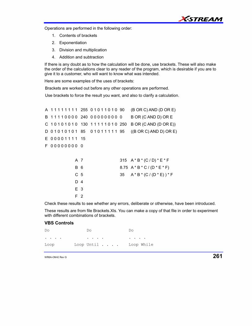
WR6A-OM-E Rev G 261
Operations are performed in the following order:
1. Contents of brackets
2. Exponentiation
3. Division and multiplication
4. Addition and subtraction
If there is any doubt as to how the calculation will be done, use brackets. These will also make the order of the calculations clear to any reader of the program, which is desirable if you are to give it to a customer, who will want to know what was intended.
Here are some examples of the uses of brackets:
Brackets are worked out before any other operations are performed.
Use brackets to force the result you want, and also to clarify a calculation.
A 1 1 1 1 1 1 1 1 255 0 1 0 1 1 0 1 0 90 (B OR C) AND (D OR E)
B 1 1 1 1 0 0 0 0 240 0 0 0 0 0 0 0 0 0 B OR (C AND D) OR E
C 1 0 1 0 1 0 1 0 130 1 1 1 1 1 0 1 0 250 B OR (C AND (D OR E))
D 0 1 0 1 0 1 0 1 85 0 1 0 1 1 1 1 1 95 ((B OR C) AND D) OR E)
E 0 0 0 0 1 1 1 1 15
F 0 0 0 0 0 0 0 0 0
A 7 315 A * B * (C / D) * E * F
B 6 8.75 A * B * C / (D * E * F)
C 5 35 A * B * (C / (D * E) ) * F
D 4
E 3
F 2
Check these results to see whether any errors, deliberate or otherwise, have been introduced.
These results are from file Brackets.Xls. You can make a copy of that file in order to experiment with different combinations of brackets.
VBS Controls Do Do Do
. . . . . . . . . . . .
Loop Loop Until . . . . Loop While
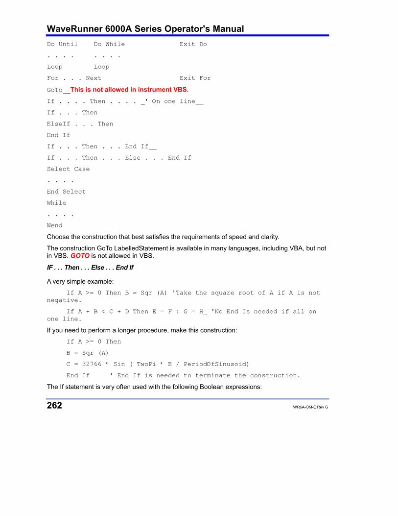
WaveRunner 6000A Series Operator's Manual
262 WR6A-OM-E Rev G
Do Until Do While Exit Do
. . . . . . . .
Loop Loop
For . . . Next Exit For
GoTo__This is not allowed in instrument VBS. If . . . . Then . . . . _' On one line__
If . . . Then
ElseIf . . . Then
End If
If . . . Then . . . End If__
If . . . Then . . . Else . . . End If
Select Case
. . . .
End Select
While
. . . .
Wend
Choose the construction that best satisfies the requirements of speed and clarity.
The construction GoTo LabelledStatement is available in many languages, including VBA, but not in VBS. GOTO is not allowed in VBS.
IF . . . Then . . . Else . . . End If
A very simple example:
If A >= 0 Then B = Sqr (A) 'Take the square root of A if A is not negative.
If A + B < C + D Then E = F : G = H_ 'No End Is needed if all on one line.
If you need to perform a longer procedure, make this construction:
If A >= 0 Then
B = Sqr (A)
C = 32766 * Sin ( TwoPi * B / PeriodOfSinusoid)
End If ' End If is needed to terminate the construction.
The If statement is very often used with the following Boolean expressions:
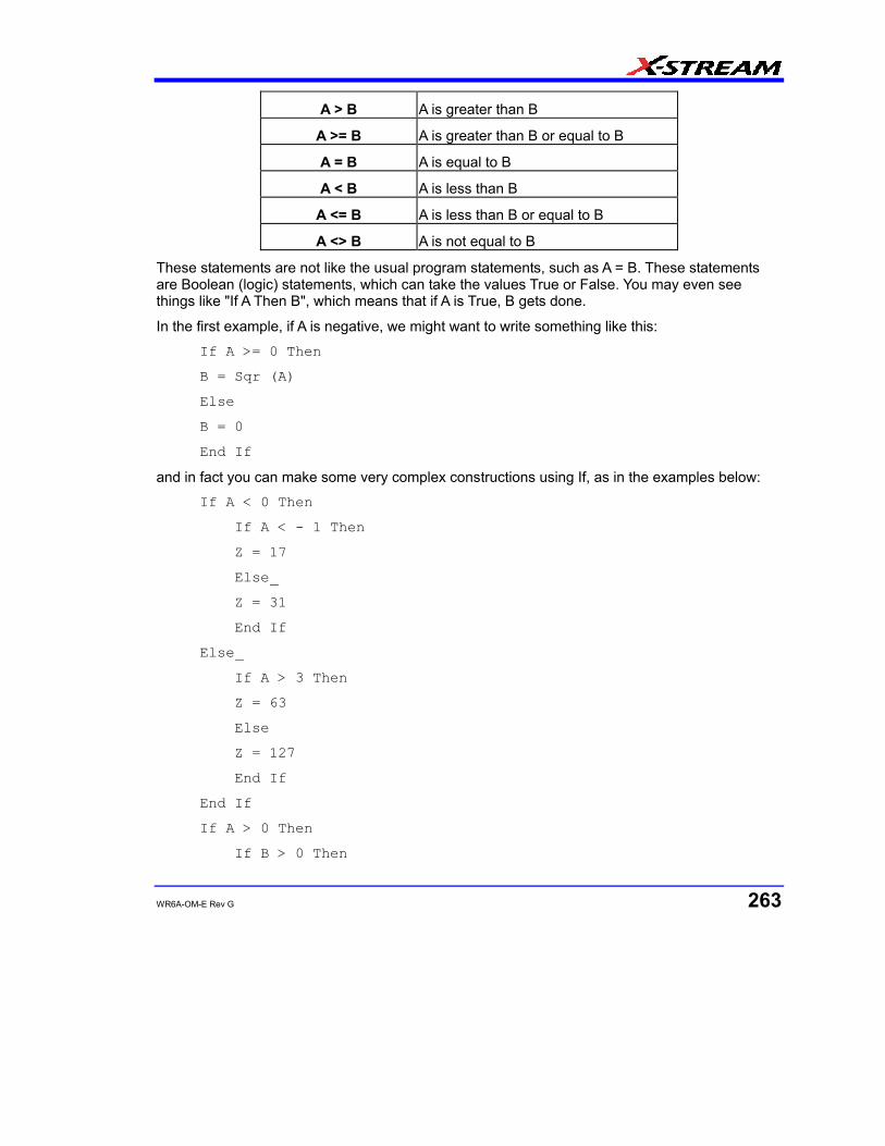
WR6A-OM-E Rev G 263
A > B A is greater than B
A >= B A is greater than B or equal to B
A = B A is equal to B
A < B A is less than B
A <= B A is less than B or equal to B
A <> B A is not equal to B
These statements are not like the usual program statements, such as A = B. These statements are Boolean (logic) statements, which can take the values True or False. You may even see things like "If A Then B", which means that if A is True, B gets done.
In the first example, if A is negative, we might want to write something like this:
If A >= 0 Then
B = Sqr (A)
Else
B = 0
End If
and in fact you can make some very complex constructions using If, as in the examples below:
If A < 0 Then
If A < - 1 Then
Z = 17
Else_
Z = 31
End If
Else_
If A > 3 Then
Z = 63
Else
Z = 127
End If
End If
If A > 0 Then
If B > 0 Then
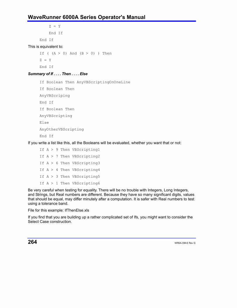
WaveRunner 6000A Series Operator's Manual
264 WR6A-OM-E Rev G
Z = Y
End If
End If
This is equivalent to:
If ( (A > 0) And (B > 0) ) Then
Z = Y
End If
Summary of If . . . . Then . . . . Else
If Boolean Then AnyVBScriptingOnOneLine
If Boolean Then
AnyVBScriping
End If
If Boolean Then
AnyVBScripting
Else
AnyOtherVBScripting
End If
If you write a list like this, all the Booleans will be evaluated, whether you want that or not:
If A > 9 Then VBScripting1
If A > 7 Then VBScripting2
If A > 6 Then VBScripting3
If A > 4 Then VBScripting4
If A > 3 Then VBScripting5
If A > 1 Then VBScripting6
Be very careful when testing for equality. There will be no trouble with Integers, Long Integers, and Strings, but Real numbers are different. Because they have so many significant digits, values that should be equal, may differ minutely after a computation. It is safer with Real numbers to test using a tolerance band.
File for this example: IfThenElse.xls
If you find that you are building up a rather complicated set of Ifs, you might want to consider the Select Case construction.
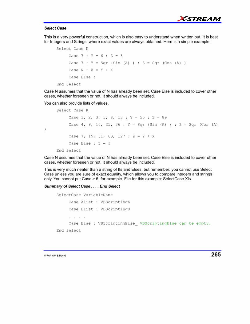
WR6A-OM-E Rev G 265
Select Case
This is a very powerful construction, which is also easy to understand when written out. It is best for Integers and Strings, where exact values are always obtained. Here is a simple example:
Select Case K
Case 7 : Y = 6 : Z = 3
Case 7 : Y = Sqr (Sin (A) ) : Z = Sqr (Cos (A) )
Case N : Z = Y + X
Case Else :
End Select
Case N assumes that the value of N has already been set. Case Else is included to cover other cases, whether foreseen or not. It should always be included.
You can also provide lists of values.
Select Case K
Case 1, 2, 3, 5, 8, 13 : Y = 55 : Z = 89
Case 4, 9, 16, 25, 36 : Y = Sqr (Sin (A) ) : Z = Sqr (Cos (A) )
Case 7, 15, 31, 63, 127 : Z = Y + X
Case Else : Z = 3
End Select
Case N assumes that the value of N has already been set. Case Else is included to cover other cases, whether foreseen or not. It should always be included.
This is very much neater than a string of Ifs and Elses, but remember: you cannot use Select Case unless you are sure of exact equality, which allows you to compare integers and strings only. You cannot put Case > 5, for example. File for this example: SelectCase.Xls
Summary of Select Case . . . . End Select
SelectCase VariableName
Case Alist : VBScriptingA
Case Blist : VBScriptingB
. . . .
Case Else : VBScriptingElse_ VBScriptingElse can be empty.
End Select

WaveRunner 6000A Series Operator's Manual
266 WR6A-OM-E Rev G
Do . . . Loop
This construction is useful when you do not know at programming time how many times the loop will be executed. Here are some examples:
Do
AnyVBSCalculation
Loop Until D > Pi
Do Until Z < Y
AnyVBSCalculation
Loop
Do
AnyVBSCalculation
Loop While D <= Pi
Do While Y >=Z
AnyVBSCalculation
Loop
These constructions enable you to make the test before or after the calculation. If before, the calculation might not be done even one time, if the condition for terminating were already true. With the condition at the end, the calculation is done at least one time.
Sometimes you might want to exit the loop from somewhere inside: for example, if some kind of problem is looming, such as the logarithm of a negative number.
For this case, you can use If . . . . Then Exit Do.
To make a pause of 10 seconds you can write:
NewTime = Timer + 10.0
Do Loop Until Timer >= NewTime
where Timer is a clock function in the PC, which has a resolution of one second.
Example file for these constructions: DoLoops.Xls
While . . . Wend
This is similar to Do While . . . Loop. You can write things like:
While ( (A > 2) And (C < 92677663) )
AnyVBCalculation
Wend
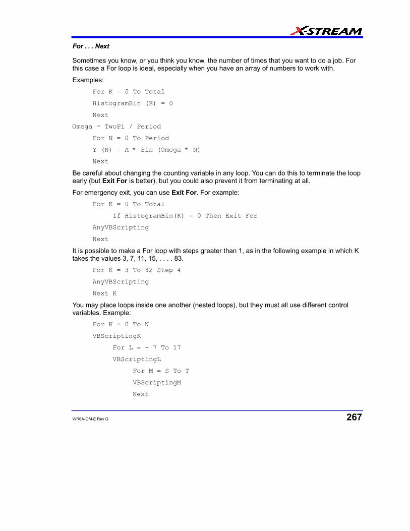
WR6A-OM-E Rev G 267
For . . . Next
Sometimes you know, or you think you know, the number of times that you want to do a job. For this case a For loop is ideal, especially when you have an array of numbers to work with.
Examples:
For K = 0 To Total
HistogramBin (K) = 0
Next
Omega = TwoPi / Period
For N = 0 To Period
Y (N) = A * Sin (Omega * N)
Next
Be careful about changing the counting variable in any loop. You can do this to terminate the loop early (but Exit For is better), but you could also prevent it from terminating at all.
For emergency exit, you can use Exit For. For example:
For K = 0 To Total
If HistogramBin(K) = 0 Then Exit For
AnyVBScripting
Next
It is possible to make a For loop with steps greater than 1, as in the following example in which K takes the values 3, 7, 11, 15, . . . . 83.
For K = 3 To 82 Step 4
AnyVBScripting
Next K
You may place loops inside one another (nested loops), but they must all use different control variables. Example:
For K = 0 To N
VBScriptingK
For L = - 7 To 17
VBScriptingL
For M = S To T
VBScriptingM
Next

WaveRunner 6000A Series Operator's Manual
268 WR6A-OM-E Rev G
Next
Next
VBS keywords and functions The ones in italics do not apply to the instrument.
+ Add two values or concatenate two strings.
- Subtract two values.
* Multiply two values.
/ Divide two values.
\ Divide two values to obtain an integer result
Abs Make absolute value.
Asc Make ASCII value of a character.
Atn Make tan-1 of a value. Result in range from -π /2 to +π /2 radians.
Cdbl Convert a value to double precision floating point.
Chr Create a character from an integer in range 0 to 255.
Cint Convert a value to nearest integer in the range -32768 to +32767
Clng Convert a value to nearest long integer in the range -231 to +231 - 1.
Close Close a file.
Cos Make the cosine of an angle expressed in radians.
Csng Convert a number to single precision floating point.
Cstr Convert a variable to a string.
Exp Raise e to the power of the input.
Get Get a value from a file.
Input Get some ASCII data from a file.
Instr Find the position of a string in a longer string.
Int Convert to nearest integer below the input value.
Left Take some characters at the left end of a string.
Log Take the natural logarithm of a positive value.
Ltrim Remove spaces at the left end of a string.
Mid Take or insert some characters in a string.
Mod Take the modulus of a value in terms of another value.

WR6A-OM-E Rev G 269
On Error Take some action if an error occurs.
Open Open a file.
Print Send some ASCII data to a file.
Put Send some data to a file.
Randomize Randomize Timer re-seeds the pseudo-random number generator.
Read Read from a file.
Right Take some characters at the right end of a string.
Rnd Make a random real number in the range from 0.0 to 1.0
Rtrim Remove spaces from right hand end of a string.
Sin Make the sine of an angle expressed in radians.
Sqr Make the square root of a positive number.
Str Make a string from a numerical value.
Timer Time since midnight in seconds, with a resolution of one second.
Trim Remove leading and trailing spaces from a string.
Val Get the ASCII value of a string beginning with numerical characters.
Other VBS Words
Const Define a constant value.
Dim Dimension a variable.
Redim Dimension a variable again.
Boolean Boolean variable
Double Double precision real variable.
Integer Integer in the range -32768 to + 32767
Long Long integer in the range -231 to + 231 - 1
Single Single precision real variable
String String variable
And Logical AND
Or Logical OR
To make a bit-by-bit comparison, logical constructions can be used with variables, as in A and B, or with tests such as If A > B Then . . .
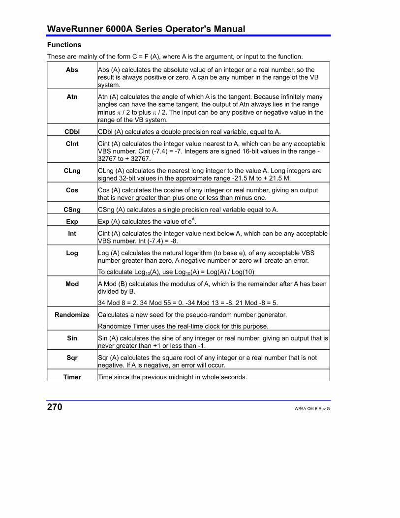
WaveRunner 6000A Series Operator's Manual
270 WR6A-OM-E Rev G
Functions These are mainly of the form C = F (A), where A is the argument, or input to the function.
Abs Abs (A) calculates the absolute value of an integer or a real number, so the result is always positive or zero. A can be any number in the range of the VB system.
Atn Atn (A) calculates the angle of which A is the tangent. Because infinitely many angles can have the same tangent, the output of Atn always lies in the range minus π / 2 to plus π / 2. The input can be any positive or negative value in the range of the VB system.
CDbl CDbl (A) calculates a double precision real variable, equal to A.
CInt Cint (A) calculates the integer value nearest to A, which can be any acceptable VBS number. Cint (-7.4) = -7. Integers are signed 16-bit values in the range -32767 to + 32767.
CLng CLng (A) calculates the nearest long integer to the value A. Long integers are signed 32-bit values in the approximate range -21.5 M to + 21.5 M.
Cos Cos (A) calculates the cosine of any integer or real number, giving an output that is never greater than plus one or less than minus one.
CSng CSng (A) calculates a single precision real variable equal to A.
Exp Exp (A) calculates the value of eA.
Int Cint (A) calculates the integer value next below A, which can be any acceptable VBS number. Int (-7.4) = -8.
Log Log (A) calculates the natural logarithm (to base e), of any acceptable VBS number greater than zero. A negative number or zero will create an error.
To calculate Log10(A), use Log10(A) = Log(A) / Log(10)
Mod A Mod (B) calculates the modulus of A, which is the remainder after A has been divided by B.
34 Mod 8 = 2. 34 Mod 55 = 0. -34 Mod 13 = -8. 21 Mod -8 = 5.
Randomize Calculates a new seed for the pseudo-random number generator.
Randomize Timer uses the real-time clock for this purpose.
Sin Sin (A) calculates the sine of any integer or real number, giving an output that is never greater than +1 or less than -1.
Sqr Sqr (A) calculates the square root of any integer or a real number that is not negative. If A is negative, an error will occur.
Timer Time since the previous midnight in whole seconds.

WR6A-OM-E Rev G 271
Hints and Tips for VBScripting • Set the trigger to Single or Stopped if you need to do a lot of editing: it is faster.
• Before starting a script, remove any existing scripts that you do not need. This is because errors in an existing script will give you error messages, even if your current script is perfect. And an existing good script may develop a fault if you change the setup. For example, you might change the vertical scale or the memory length and get an overflow if you did not guard against it in the script.
• When starting a script, make sure that you have chosen the right kind: function or parameter. You can get some very frustrating problems if you are in the wrong mode. You can cut and paste the VBS statements if you discover this error.
• If your calculation requires a long memory, development might be quicker if you test the principles on a shorter trace at first.
• Note that the pseudo-random number generator is reset at the start of a script. If you want a different set of pseudo-randoms every time, put Randomize Timer in the program, to be run once, before any pseudo-randoms are generated. You can use this instruction to re-seed the generator at any time during execution.
• Do not put the final statement in a loop, hoping that you can see a progressive result as some parameter changes. No output will be seen on the screen of the instrument until the script has been completely run and quitted, so only the final result will appear. If the loop runs many times, you will think that the scope has hung up.
• If you want a For loop, end it with "Next" and not "Next X".
• If you make a script that takes a long time to run, go back to the default setup before quitting or powering down, or you will have a long wait next time you power up.
• Always use a recursive calculation when this will speed things up.
• Keep everything outside a loop that does not have to be inside, to speed things up.
• Make your scripts clear, not only by indenting and commenting, but by structuring neatly as well.
• Sometimes it might be easier to develop your script in Excel VBA (remembering that VBA is not identical to VBS), so that you can display intermediate results. If you do this, note that you can read from a cell or write to it using statements like these:
A = Worksheets("Sheet1").Cells(Row, Column).Value
Worksheets("Sheet1").Cells(Row, Column).Value = B
• Note that in VBS, after you have corrected an error and clicked on "Apply," the error message may go on flashing for a few seconds, or a few acquisitions, before being erased. Look for the "Script OK" message. Be patient before assuming that you still have a bug.
WaveRunner 6000A Series Operator's Manual
272 WR6A-OM-E Rev G
• If your calculation requires data to be used at some other horizontal positions than their original ones, make sure that your algorithm does not try to send data to non-existent array positions, that is, beyond the edges of the screen. You may have to truncate your output trace, as happens with the instrument's Enhanced Resolution and Boxcar functions.
• No output will emerge from a script until you press Apply.
• No output will emerge from a script until it has received an input. This includes the case where the input data are not used in calculating the output data. So you must have had at least one acquisition before you see anything.
• Because you can introduce undeclared variables at any point in a calculation, VBS does not check your spelling.
• You can make a portion of a trace disappear if you set the values to 32767 or -32768.
• You can highlight a section of a trace by making the points alternately too high and too low by a suitable amount. Providing the memory length is not too short, the compaction algorithm will give the effect of a thicker trace.
• The lengths of the output trace and the input trace need not be the same. You can even make the output trace longer than the input trace, but you will need to unzoom it to see it all. This feature can be used to avoid compaction problems with non-linear horizontal scales. It can also be used to show several versions of a function at the same time, without having to set up a separate script for each one.
• If your program structure is complicated, consider typing all the IFs, ELSEIFs, ENDIFs, FORs, NEXTs, etc and then clicking Apply. You wont get any output, but the system will tell you if the structure is acceptable. Then you can insert the actual program statements.
• Always try to make the script as independent as possible of variables such as V/Div, T/Div, and memory length, unless that would make it harder to understand. If so, give some values as examples, and explain how the script would have to change if the variables changed.
ERRORS The instrument VBS tries hard to help you when errors occur.
Errors may be of two main types:
• The script may not be usable because the interpreter cannot construct a logical structure from it.
• The script may be usable, but may fail while running because an incomputable function has been requested.
Sometimes the line number given for an error is wrong. This can happen when the error is of this general type:
Missing "Next" Missing "End If"
Extra "Next" Missing "Until" etc.
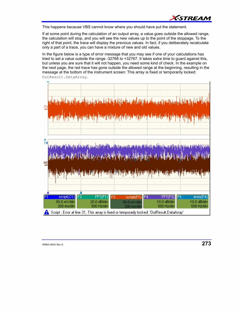
WR6A-OM-E Rev G 273
This happens because VBS cannot know where you should have put the statement.
If at some point during the calculation of an output array, a value goes outside the allowed range, the calculation will stop, and you will see the new values up to the point of the stoppage. To the right of that point, the trace will display the previous values. In fact, if you deliberately recalculate only a part of a trace, you can have a mixture of new and old values.
In the figure below is a type of error message that you may see if one of your calculations has tried to set a value outside the range -32768 to +32767. It takes extra time to guard against this, but unless you are sure that it will not happen, you need some kind of check. In the example on the next page, the red trace has gone outside the allowed range at the beginning, resulting in the message at the bottom of the instrument screen: This array is fixed or temporarily locked: OutResult.DataArray.
WaveRunner 6000A Series Operator's Manual
274 WR6A-OM-E Rev G
Error Handling Note that the construction OnError GoTo Label: is not allowed in VBS. In fact no GoTos or labels are allowed. Therefore there is no way for you to provide handlers to deal with errors and exceptions. You must be aware of all possibilities at all points in your program, and you must either be certain that errors will not occur, or you must take action to ensure that they do not.
Examples:
Sqr You cannot take the square root of a negative number.
Log You cannot take the log of zero or of a negative number.
A / B You cannot divide by zero.
Array You cannot use an index outside the bounds of an array.
Size Unscaled data cannot go outside the range -32768 to 32767.
If there is any possibility that any of these might occur, take steps to deal with this before it can happen.
For example, you may write some kind of generator of pseudo-random statistical values. If these belong to a distribution that in principle has an infinite range, or a finite range which is wider than the signed 16-bits allowed, check each value. If a value falls outside the range, you could set it to the maximum or generate another example.
You can, however, use one of the following: On Error Resume Next
followed by some code that may make some attempt to deal with the problem, or at least to allow execution to continue.
On Error GoTo 0
This cancels On Error Resume Next_
Speed of Execution To maximize the speed of execution of a script, the most important thing you can do is to minimize the number of operations that are performed inside loops. Anything done once only is unlikely to be an important source of delay. Please note that VBS is much slower than the internal computations of the instrument, so do everything you can to save time, unless time is irrelevant to the application.
Using an array element takes longer than using a single variable. Here is an example:
For K = 1 to Total
If X (K) > X (K - 1) Then
Y = Cos (X (K) ) * Sin (X (K) ) * Sqr (X (K) )
End If

WR6A-OM-E Rev G 275
Next
To do the same thing we could also write this, using the index only once:
OldXK = X (0)
For K = 1 To Total
XK = X (K)
If XK > OldXK Then
Y = Cos (XK) * Sin (XK) * Sqr (XK)
OldXK = XK
End If
Next
VBS runs slower than the "internal" calculations, because the scripts are interpreted. This could be serious for calculations where many operations are needed on each sample, such as convolution, correlation, and long digital filters.
Scripting Ideas What can we do in a VBS script that we cannot do with the normal instrument functions? Here are some possibilities.
• Create a new function that acts on waveform values.
• Create a new parameter.
• Create a new form of non-linear vertical scale.
• Create a new form of non-linear horizontal scale.
• Move some or all data horizontally, including reflections.
• Combine data to form digital filters.
• Show several function results side by side.
• Show several function results interleaved.
You can even create output data that are not related to the input. The output data need not even be in the same domain as the input data, because the system treats them as pure numbers. So you can create your own transforms into the frequency domain, for example.
Example Waveform Script • Custom Window
• Creating a window function for FFT calculations.
WaveRunner 6000A Series Operator's Manual
276 WR6A-OM-E Rev G
Example Parameter Scripts • Decay Parameter
• Calculating the rate of decay of a damped sine.
• Locating Pulses
• Finding pulses in a pulse train.
Debugging Scripts Until we have integrated a more comprehensive debugger for VBScript there is a workaround.
1. Download the Windows Scripting Debugger for Windows 2000 from here:
http://download.microsoft.com/download/winscript56/Install/1.0a/NT45XP/EN-US/scd10en.exe
2. Enable JIT (Just In Time) debugging by setting the following registry key
HKCU\Software\Microsoft\Windows Script\Settings\JITDebug = to 1 (DWORD value)
3. Place a Stop statement in your script.
Now, when the Stop statement is executed the debugger will open and allow single-stepping, variable examination, etc.
Using VBA or Visual Basic to debug VBScripts is not recommended since the language syntax for these three variants of basic is slightly different.
Horizontal Control Variables InResult.HorizontalOffset Double precision Time shift of input waveform on grid in
units of horizontal scale
OutResult.HorizontalOffset Double precision Time shift of output waveform on grid in units of horizontal scale
InResult.HorizontalPerStep Double precision Time between successive samples in the input waveform
OutResult.HorizontalPerStep Double precision Time between successive samples in the output waveform
InResult.HorizontalUnits String Horizontal units of input waveform
OutResult.HorizontalUnits String Horizontal units of output waveform
InResult.Samples Integer Number of samples in input waveform
Vertical Control Variables InResult.VerticalOffset Double precision Vertical shift of input waveform on grid
OutResult.VerticalOffset Double precision Vertical shift of output waveform on grid
WR6A-OM-E Rev G 277
InResult.VerticalPerStep Double precision Difference between successive possible levels in the input waveform memory
OutResultVerticalPerStep Double precision Difference between successive possible levels in the output waveform memory
1 / 65536 of vertical full scale
InResult.VerticalResolution Double precision Difference between successive possible physical levels in the input waveform
OutResultVerticalResolution Double precision Difference between successive possible physical levels in the output waveform
1 / 256 of vertical full scale for channel waveforms
1 / 65536 of vertical full scale for math waveforms
InResult.VerticalUnits String Vertical units of input waveform
OutResult.VerticalUnits String Vertical units of output waveform
List of Variables Available to Scripts FirstEventTime([out, retval] VARIANT * pVal); FirstEventTime([in] VARIANT newVal);
LastEventTime([out, retval] VARIANT * pVal); LastEventTime([in] VARIANT newVal);
UpdateTime([out, retval] VARIANT * pVal); UpdateTime([in] VARIANT newVal);
Details([in] BSTR strDetailsIID, [out, retval] VARIANT * pVal);
Status([out, retval] VARIANT * pVal); Status([in] VARIANT newVal);
ExtendedStatus([out, retval] VARIANT * pVal); ExtendedStatus([in] VARIANT newVal);
StatusDescription([out, retval] BSTR * pVal); StatusDescription([in] BSTR newVal);
DataArray([in, defaultvalue(TRUE)] BOOL arrayValuesScaled,
[in, defaultvalue(LEC_ALL_DATA)] int numSamples,
[in, defaultvalue(0)] int startIndex,
[in, defaultvalue(1)] int sparsingFactor,
[out, retval] VARIANT *pArray);
DataArray([in, defaultvalue(TRUE)] BOOL arrayValuesScaled,
[in, defaultvalue(LEC_ALL_DATA)] int numSamples,
[in, defaultvalue(0)] int startIndex,
[in, defaultvalue(1)] int sparsingFactor,
WaveRunner 6000A Series Operator's Manual
278 WR6A-OM-E Rev G
[in] VARIANT array);
HorizontalUnits([out, retval] BSTR *pVal); HorizontalUnits([in] BSTR newVal);
Samples([out, retval] int *pVal); Samples([in] int newVal);
HorizontalResolution([out, retval] double *pVal); HorizontalResolution([in] double newVal);
HorizontalPerStep([out, retval] double *pVal); HorizontalPerStep([in] double newVal);
HorizontalOffset([out, retval] double *pVal); HorizontalOffset([in] double newVal);
Sweeps([out, retval] int *pVal); Sweeps([in] int newVal);
HorizontalVariances([out, retval] int *pVal); HorizontalVariances([in] int newVal);
HorizontalVarianceArray([out, retval] VARIANT * pArray);
HorizontalVarianceArray([in] VARIANT array);
HorizontalFrameStart([out, retval] double *pVal); HorizontalFrameStart([in] double newVal);
HorizontalFrameStop([out, retval] double *pVal); HorizontalFrameStop([in] double newVal);
VerticalFrameStart([out, retval] double *pVal); VerticalFrameStart([in] double newVal);
VerticalFrameStop([out, retval] double *pVal); VerticalFrameStop([in] double newVal);
VerticalResolution([out, retval] double *pVal); VerticalResolution([in] double newVal);
VerticalPerStep([out, retval] double *pVal); VerticalPerStep([in] double newVal);
VerticalOffset([out, retval] double *pVal); VerticalOffset([in] double newVal);
VerticalMinPossible([out, retval] double *pVal); VerticalMinPossible([in] double newVal);
VerticalMaxPossible([out, retval] double *pVal); VerticalMaxPossible([in] double newVal);
VerticalUnits([out, retval] BSTR *pVal); VerticalUnits([in] BSTR newVal);
Communicating with Other Programs from a VBScript
The ability of The instrument to communicate with other programs opens up immense possibilities, both for calculation and for graphics, making the assembly of reports relatively simple.
Communicating with Excel from a VBScript Although there are direct instrument calls to Excel and other programs, you may wish to do this from a VBScript. Here is an example:
OutResult.Samples = InResult.Samples
startData = 0
endData = OutResult.Samples
ReDim newData(OutResult.Samples)
USD = InResult.DataArray(False)

WR6A-OM-E Rev G 279
LastPoint = endData - 1
Set ExcelApp = GetObject(,"Excel.Application")
ExcelApp.Visible = True
ExcelColumnA = 2 'Column where the data will appear in Excel
ExcelRow = 10 'Row where the data will start
ExcelColumnB = 3 ' Column where the output data will appear in Excel
For K = 0 To LastPoint
ExcelApp.ActiveSheet.Cells("ExcelRow + K, ExcelColumnA ") = -USD(K)
Next
Once the data are in Excel, any Excel functions can be applied to the data. The results can be returned to the VB script.
For K = 0 To LastPoint
NDA(K) = ExcelApp.ActiveSheet.Cells("ExcelRow + K, ExcelColumnB")
Next
Transferring data cell by cell is very slow, so it is better to do a block transfer.
Calling MATLAB from the Instrument Calling MATLAB Note: Load MATLAB version 6.5 just as you would on any PC. Once it is loaded, open MATLAB from the desktop, then close it again, before you attempt to open it from the instrument application. This is to update the registry.
MATLAB can be directly called from the instrument in two ways:
Using a function F1 through Fx The number of math traces available depends on the software options loaded on your scope. See Specifications.
MATLAB returns a waveform
Using a parameter P1 through Px MATLAB returns a parameter
In both cases, one call to MATLAB can use two separate waveforms as input, providing much greater computing power than is available by calling MATLAB from a VBScript. Note: If you do not place a semicolon ";" at the end of a line, MATLAB will show the calculated value in the result window, significantly slowing down the processing rate. This feature is best kept for diagnostics.
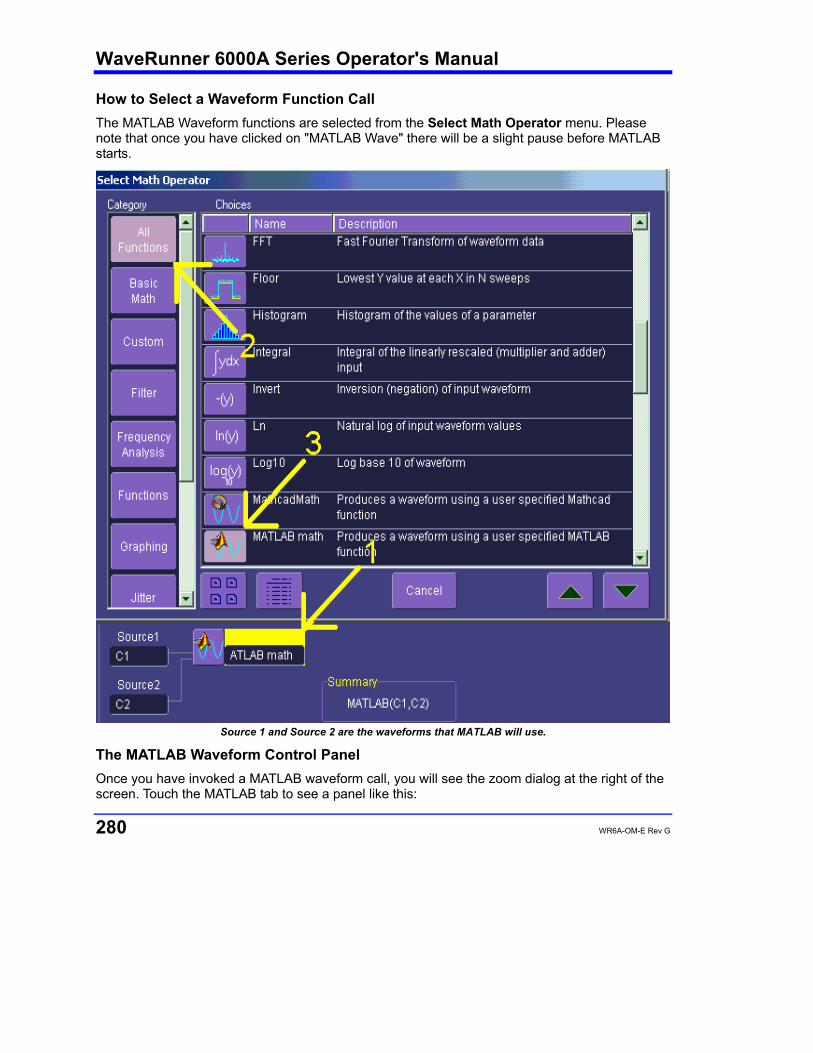
WaveRunner 6000A Series Operator's Manual
280 WR6A-OM-E Rev G
How to Select a Waveform Function Call The MATLAB Waveform functions are selected from the Select Math Operator menu. Please note that once you have clicked on "MATLAB Wave" there will be a slight pause before MATLAB starts.
Source 1 and Source 2 are the waveforms that MATLAB will use.
The MATLAB Waveform Control Panel Once you have invoked a MATLAB waveform call, you will see the zoom dialog at the right of the screen. Touch the MATLAB tab to see a panel like this:
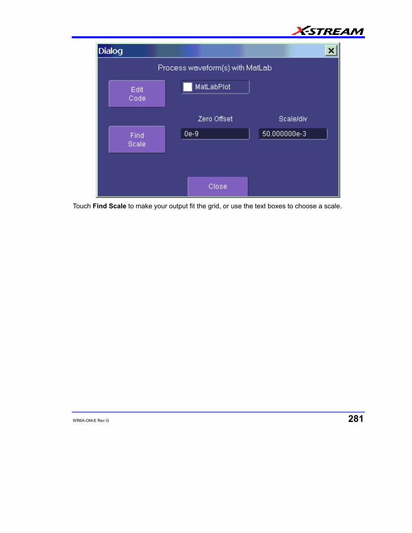
WR6A-OM-E Rev G 281
Touch Find Scale to make your output fit the grid, or use the text boxes to choose a scale.
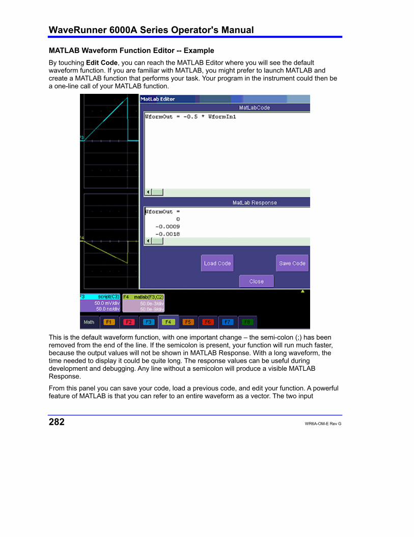
WaveRunner 6000A Series Operator's Manual
282 WR6A-OM-E Rev G
MATLAB Waveform Function Editor -- Example By touching Edit Code, you can reach the MATLAB Editor where you will see the default waveform function. If you are familiar with MATLAB, you might prefer to launch MATLAB and create a MATLAB function that performs your task. Your program in the instrument could then be a one-line call of your MATLAB function.
This is the default waveform function, with one important change – the semi-colon (;) has been removed from the end of the line. If the semicolon is present, your function will run much faster, because the output values will not be shown in MATLAB Response. With a long waveform, the time needed to display it could be quite long. The response values can be useful during development and debugging. Any line without a semicolon will produce a visible MATLAB Response.
From this panel you can save your code, load a previous code, and edit your function. A powerful feature of MATLAB is that you can refer to an entire waveform as a vector. The two input

WR6A-OM-E Rev G 283
waveforms are WformIn1 and WformIn2, while the output is WformOut. You can also refer to individual samples, such as WformIn1(34), and sequences of samples, such as WformIn(55:89)
You can write statements such as these:
WformOut(5) = WformIn(5)
WformOut(89) = WformIn(144)
WformOut(34:55) = WformIn(34:55)
WformOut(233:377) = WformIn(100:244)
This very simple example adds a rescaled copy of Channel 2 to a copy of Channel 1, and then rescales the result.
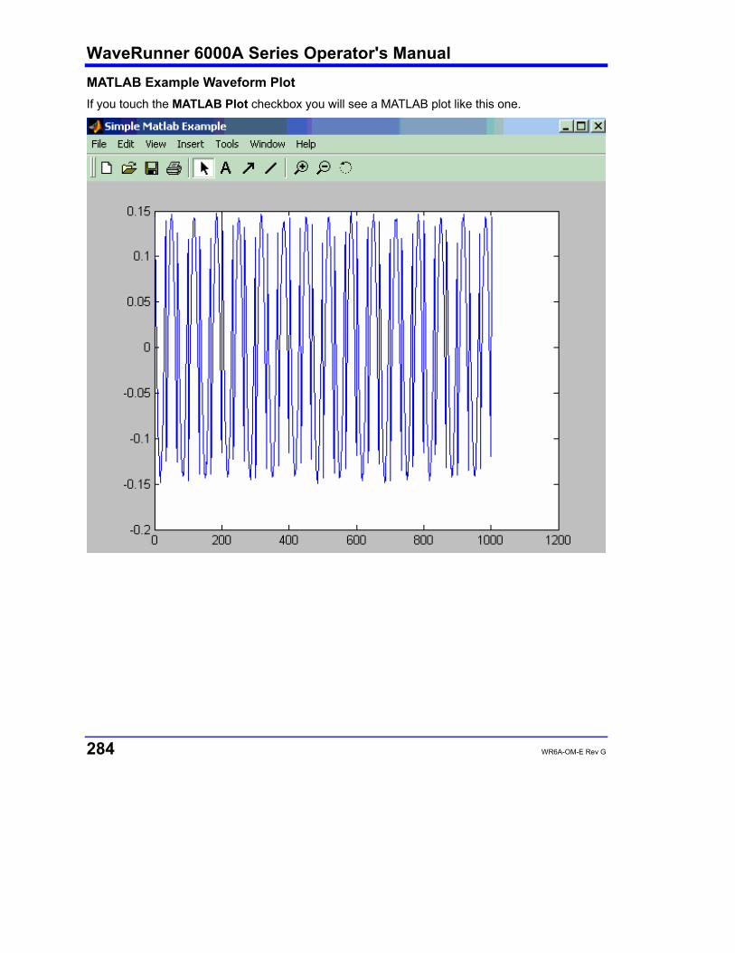
WaveRunner 6000A Series Operator's Manual
284 WR6A-OM-E Rev G
MATLAB Example Waveform Plot If you touch the MATLAB Plot checkbox you will see a MATLAB plot like this one.

WR6A-OM-E Rev G 285
How to Select a MATLAB Parameter Call
Menu position for MATLAB parameter call in Select Measurement menu.
The MATLAB Parameter Control Panel Once you have invoked a MATLAB parameter call, a mini-dialog to the right of the main dialog will appear:
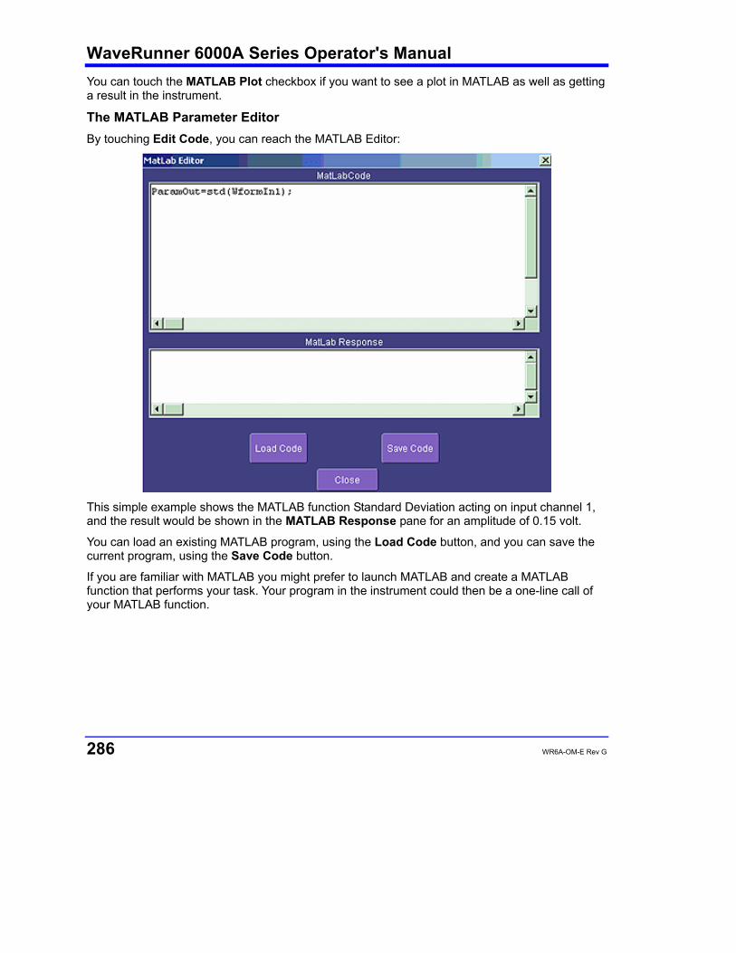
WaveRunner 6000A Series Operator's Manual
286 WR6A-OM-E Rev G
You can touch the MATLAB Plot checkbox if you want to see a plot in MATLAB as well as getting a result in the instrument.
The MATLAB Parameter Editor By touching Edit Code, you can reach the MATLAB Editor:
This simple example shows the MATLAB function Standard Deviation acting on input channel 1, and the result would be shown in the MATLAB Response pane for an amplitude of 0.15 volt.
You can load an existing MATLAB program, using the Load Code button, and you can save the current program, using the Save Code button.
If you are familiar with MATLAB you might prefer to launch MATLAB and create a MATLAB function that performs your task. Your program in the instrument could then be a one-line call of your MATLAB function.
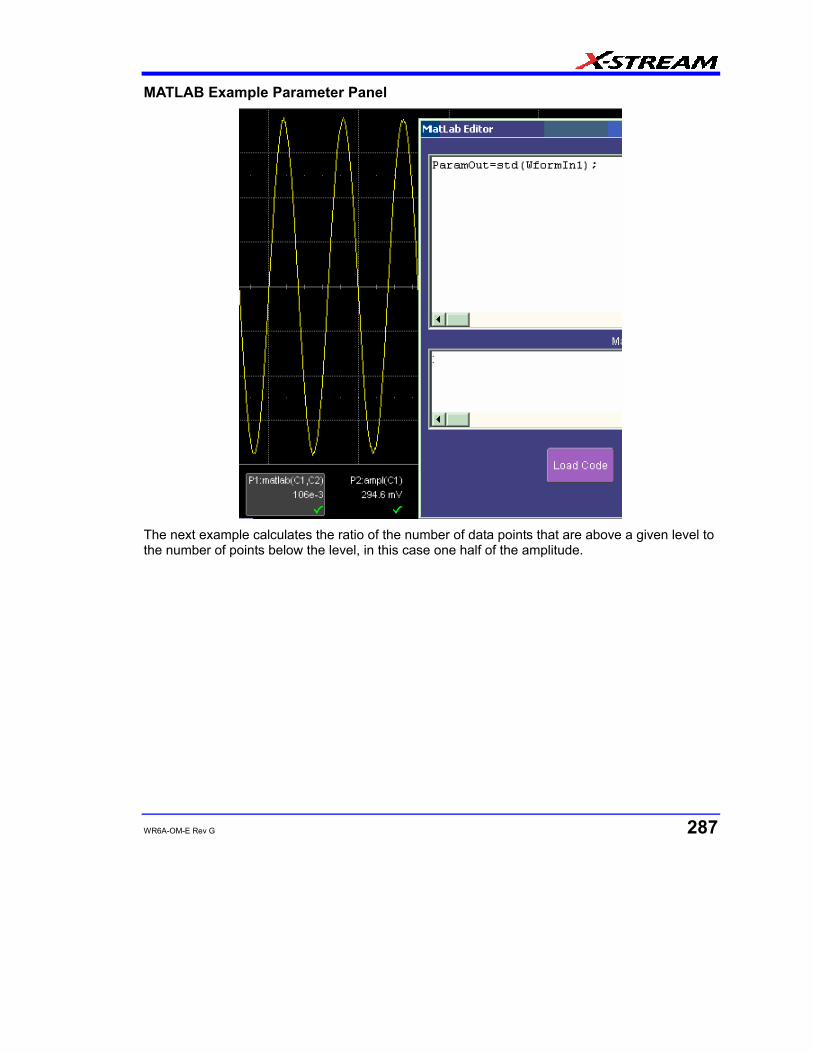
WR6A-OM-E Rev G 287
MATLAB Example Parameter Panel
The next example calculates the ratio of the number of data points that are above a given level to the number of points below the level, in this case one half of the amplitude.
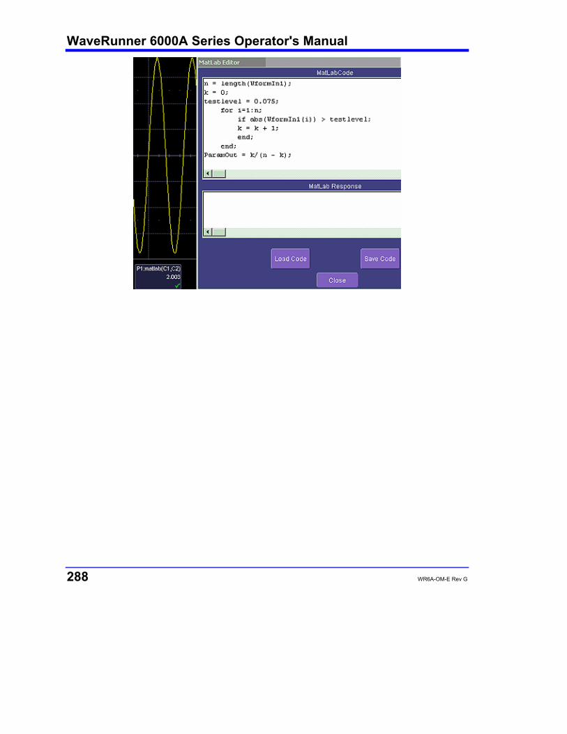
WaveRunner 6000A Series Operator's Manual
288 WR6A-OM-E Rev G
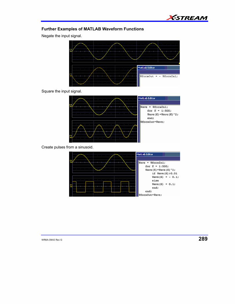
WR6A-OM-E Rev G 289
Further Examples of MATLAB Waveform Functions Negate the input signal.
Square the input signal.
Create pulses from a sinusoid.
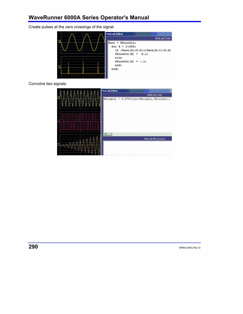
WaveRunner 6000A Series Operator's Manual
290 WR6A-OM-E Rev G
Create pulses at the zero crossings of the signal.
Convolve two signals.
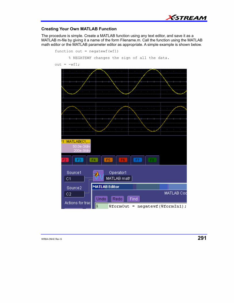
WR6A-OM-E Rev G 291
Creating Your Own MATLAB Function The procedure is simple. Create a MATLAB function using any text editor, and save it as a MATLAB m-file by giving it a name of the form Filename.m. Call the function using the MATLAB math editor or the MATLAB parameter editor as appropriate. A simple example is shown below.
function out = negatewf(wf1)
% NEGATEWF changes the sign of all the data.
out = -wf1;
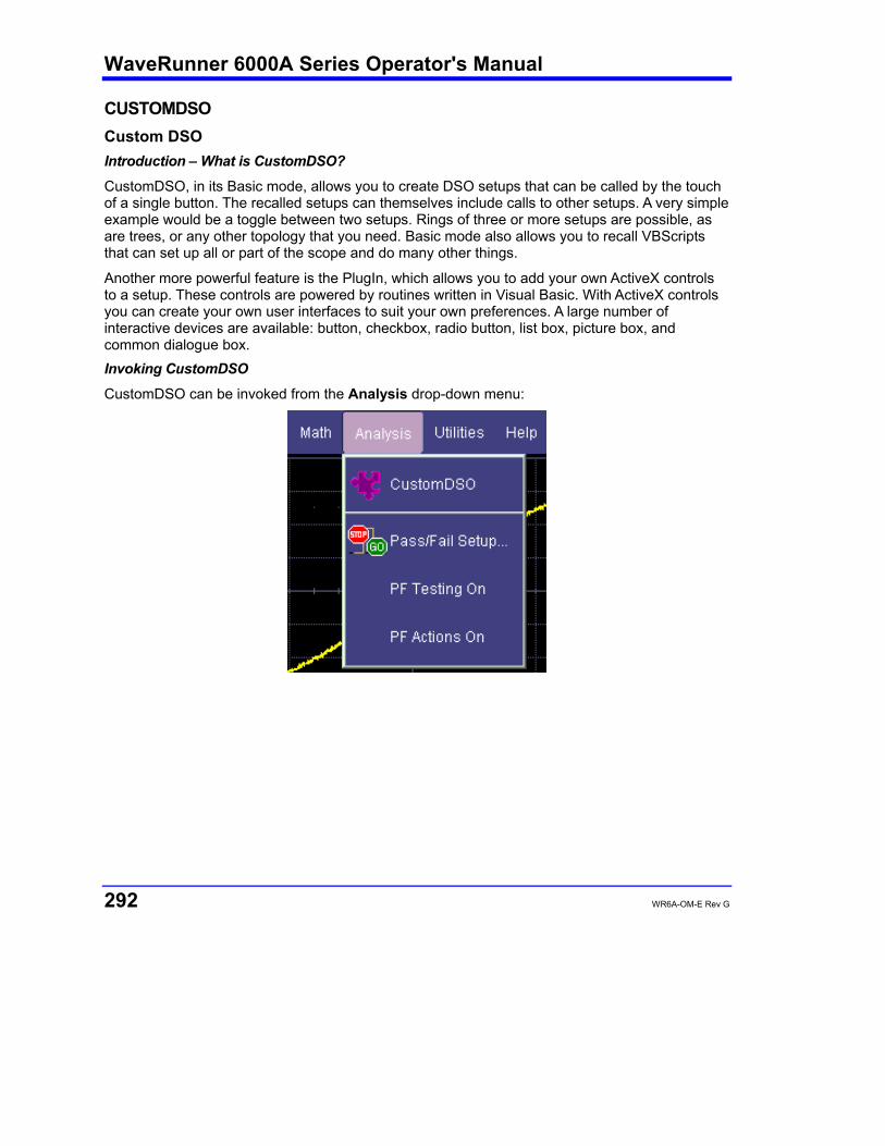
WaveRunner 6000A Series Operator's Manual
292 WR6A-OM-E Rev G
CUSTOMDSO Custom DSO Introduction – What is CustomDSO?
CustomDSO, in its Basic mode, allows you to create DSO setups that can be called by the touch of a single button. The recalled setups can themselves include calls to other setups. A very simple example would be a toggle between two setups. Rings of three or more setups are possible, as are trees, or any other topology that you need. Basic mode also allows you to recall VBScripts that can set up all or part of the scope and do many other things.
Another more powerful feature is the PlugIn, which allows you to add your own ActiveX controls to a setup. These controls are powered by routines written in Visual Basic. With ActiveX controls you can create your own user interfaces to suit your own preferences. A large number of interactive devices are available: button, checkbox, radio button, list box, picture box, and common dialogue box. Invoking CustomDSO
CustomDSO can be invoked from the Analysis drop-down menu:
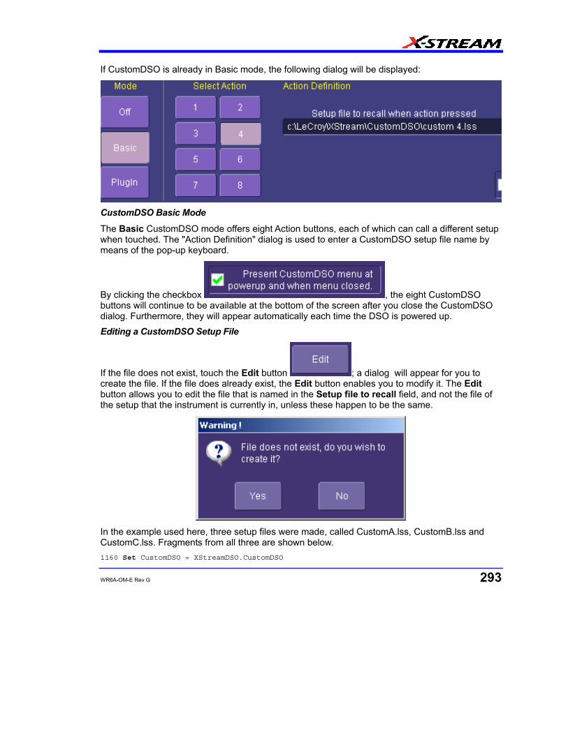
WR6A-OM-E Rev G 293
If CustomDSO is already in Basic mode, the following dialog will be displayed:
CustomDSO Basic Mode
The Basic CustomDSO mode offers eight Action buttons, each of which can call a different setup when touched. The "Action Definition" dialog is used to enter a CustomDSO setup file name by means of the pop-up keyboard.
By clicking the checkbox , the eight CustomDSO buttons will continue to be available at the bottom of the screen after you close the CustomDSO dialog. Furthermore, they will appear automatically each time the DSO is powered up. Editing a CustomDSO Setup File
If the file does not exist, touch the Edit button ; a dialog will appear for you to create the file. If the file does already exist, the Edit button enables you to modify it. The Edit button allows you to edit the file that is named in the Setup file to recall field, and not the file of the setup that the instrument is currently in, unless these happen to be the same.
In the example used here, three setup files were made, called CustomA.lss, CustomB.lss and CustomC.lss. Fragments from all three are shown below. 1160 Set CustomDSO = XStreamDSO.CustomDSO
WaveRunner 6000A Series Operator's Manual
294 WR6A-OM-E Rev G
1161 ‘ CustomDSO Setup A.lss 1162 CustomDSO.ActionScript1 = “c:\LeCroy\XStream\CustomDSO\A.lss” 1163 CustomDSO.ActionEnable1 = False 1164 CustomDSO.ActionScript1 = “c:\LeCroy\XStream\CustomDSO\B.lss” 1165 CustomDSO.ActionEnable1 = True 1166 CustomDSO.ActionScript1 = “c:\LeCroy\XStream\CustomDSO\C.lss” 1167 CustomDSO.ActionEnable1 = True 1168 CustomDSO.ActionScript1 = “c:\LeCroy\XStream\CustomDSO\A.lss” 1169 CustomDSO.ActionEnable1 = False 1160 Set CustomDSO = XStreamDSO.CustomDSO 1161 ‘ CustomDSO Setup B.lss 1162 CustomDSO.ActionScript1 = “c:\LeCroy\XStream\CustomDSO\A.lss” 1163 CustomDSO.ActionEnable1 = True 1164 CustomDSO.ActionScript1 = “c:\LeCroy\XStream\CustomDSO\B.lss” 1165 CustomDSO.ActionEnable1 = False 1166 CustomDSO.ActionScript1 = “c:\LeCroy\XStream\CustomDSO\C.lss” 1167 CustomDSO.ActionEnable1 = True 1168 CustomDSO.ActionScript1 = “c:\LeCroy\XStream\CustomDSO\A.lss” 1169 CustomDSO.ActionEnable1 = False 1160 Set CustomDSO = XStreamDSO.CustomDSO 1161 ‘ CustomDSO Setup C.lss 1162 CustomDSO.ActionScript1 = “c:\LeCroy\XStream\CustomDSO\A.lss” 1163 CustomDSO.ActionEnable1 = True 1164 CustomDSO.ActionScript1 = “c:\LeCroy\XStream\CustomDSO\B.lss” 1165 CustomDSO.ActionEnable1 = True 1166 CustomDSO.ActionScript1 = “c:\LeCroy\XStream\CustomDSO\C.lss” 1167 CustomDSO.ActionEnable1 = False 1168 CustomDSO.ActionScript1 = “c:\LeCroy\XStream\CustomDSO\A.lss” 1169 CustomDSO.ActionEnable1 = False The text in green following a single quotation mark is a VBS comment and causes no action.
The text in red contains the path and name of the setup file associated with the numbered button. This setup will be called when the button is pressed.
The boolean (in blue) decides whether the action button will invoke the setup or remain inactive.
For example, in setup B, A.lss and C.lss can be invoked, but not B, which is already in place.
As you see from the line numbers in the program fragments, the setup files are rather long because they include all the information needed to set the DSO to the required state. But if you want to make a very short file that changes only a few variables (for example, the action button settings) you can make a file that includes only the relevant instructions. This usage assumes that the remainder of the DSO is already in the required state. This is an example of the complete compatibility of the instrument's software. The same commands can be used in setups, in scripts, or in remote control commands in external programs, whether resident in the instrument or in an external computer.

WR6A-OM-E Rev G 295
Creating a CustomDSO Setup File
If you touch the Edit button when the Setup file to recall field contains the name of a non-existent file, you will see a message like this:
If you then touch Yes, the DSO will display a file like this: ' XStreamDSO ConfigurationVBScript ... ' Created by CustomDSO ... On Error Resume Next set dso = CreateObject("LeCroy.XStreamDSO.1") ' dso.Display.GridMode = "Dual" ' dso.Acquisition.C1.VerScale = 0.1 ' dso.Acquisition.Horizontal.HorScale = 1e-6 ' dso.Acquisition.TriggerMode = "Auto" You can add to this fragment any commands you need. CustomDSO PlugIn Mode
This is the mode in which CustomDSO really shows its power. You can insert any ActiveX control or graph. Creating a CustomDSO PlugIn
Follow these steps to create an example Visual Basic PlugIn:
Start a new VB project. Select ActiveX Control from the New tab.
Resize the control. A. In the Properties window set Width 11940. B. In the Properties window set Height 2475.
Place two buttons on the control. A. Double click on the command button at left of screen (left arrow below). B. Move and resize the resulting button as required, using the handles (right arrow below). C. Repeat for the second button. D. In the Properties window set the Name properties to SingleButton and AutoButton, respectively. E. Set the button Caption properties to Single and Auto, respectively
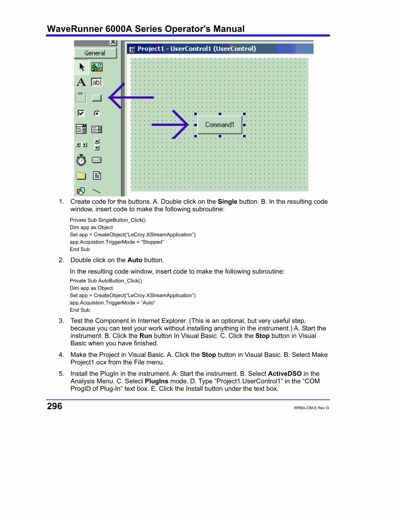
WaveRunner 6000A Series Operator's Manual
296 WR6A-OM-E Rev G
1. Create code for the buttons. A. Double click on the Single button. B. In the resulting code
window, insert code to make the following subroutine: Private Sub SingleButton_Click() Dim app as Object Set app = CreateObject(“LeCroy.XStreamApplication”) app.Acquistion.TriggerMode = “Stopped” End Sub
2. Double click on the Auto button.
In the resulting code window, insert code to make the following subroutine: Private Sub AutoButton_Click() Dim app as Object Set app = CreateObject(“LeCroy.XStreamApplication”) app.Acquistion.TriggerMode = “Auto” End Sub
3. Test the Component in Internet Explorer. (This is an optional, but very useful step, because you can test your work without installing anything in the instrument.) A. Start the instrument. B. Click the Run button In Visual Basic. C. Click the Stop button in Visual Basic when you have finished.
4. Make the Project in Visual Basic. A. Click the Stop button in Visual Basic. B. Select Make Project1.ocx from the File menu.
5. Install the PlugIn in the instrument. A. Start the instrument. B. Select ActiveDSO in the Analysis Menu. C. Select PlugIns mode. D. Type “Project1.UserControl1” in the “COM ProgID of Plug-In” text box. E. Click the Install button under the text box.
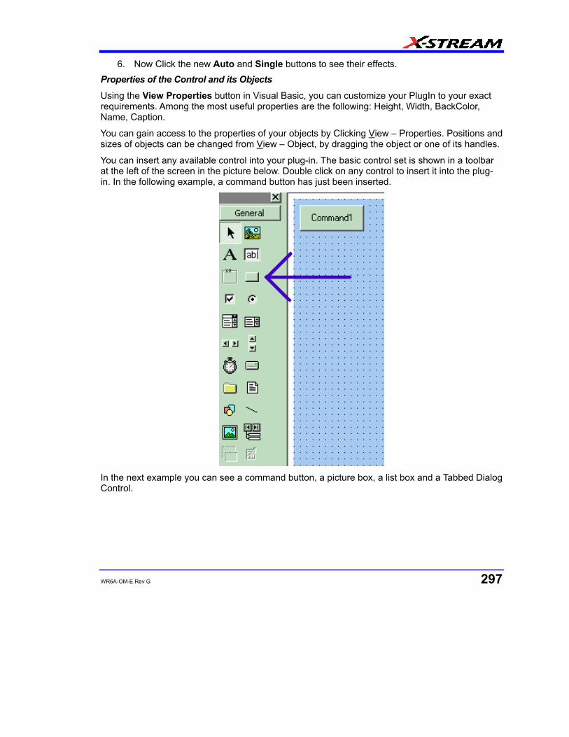
WR6A-OM-E Rev G 297
6. Now Click the new Auto and Single buttons to see their effects. Properties of the Control and its Objects
Using the View Properties button in Visual Basic, you can customize your PlugIn to your exact requirements. Among the most useful properties are the following: Height, Width, BackColor, Name, Caption.
You can gain access to the properties of your objects by Clicking View – Properties. Positions and sizes of objects can be changed from View – Object, by dragging the object or one of its handles.
You can insert any available control into your plug-in. The basic control set is shown in a toolbar at the left of the screen in the picture below. Double click on any control to insert it into the plug-in. In the following example, a command button has just been inserted.
In the next example you can see a command button, a picture box, a list box and a Tabbed Dialog Control.
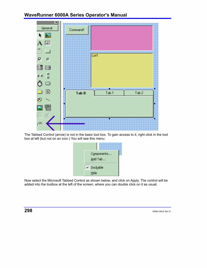
WaveRunner 6000A Series Operator's Manual
298 WR6A-OM-E Rev G
The Tabbed Control (arrow) is not in the basic tool box. To gain access to it, right click in the tool box at left (but not on an icon.) You will see this menu:
Now select the Microsoft Tabbed Control as shown below, and click on Apply. The control will be added into the toolbox at the left of the screen, where you can double click on it as usual.
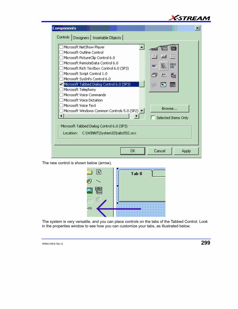
WR6A-OM-E Rev G 299
The new control is shown below (arrow).
The system is very versatile, and you can place controls on the tabs of the Tabbed Control. Look in the properties window to see how you can customize your tabs, as illustrated below.
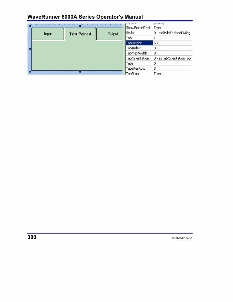
WaveRunner 6000A Series Operator's Manual
300 WR6A-OM-E Rev G
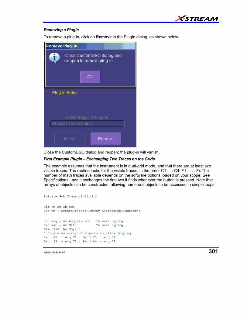
WR6A-OM-E Rev G 301
Removing a PlugIn
To remove a plug-in, click on Remove in the PlugIn dialog, as shown below:
Close the CustomDSO dialog and reopen; the plug-in will vanish. First Example PlugIn – Exchanging Two Traces on the Grids
The example assumes that the instrument is in dual-grid mode, and that there are at least two visible traces. The routine looks for the visible traces, in the order C1 . . . C4, F1 . . . . Fx The number of math traces available depends on the software options loaded on your scope. See Specifications., and it exchanges the first two it finds whenever the button is pressed. Note that arrays of objects can be constructed, allowing numerous objects to be accessed in simple loops.
Private Sub Command1_Click() Dim wm As Object Set wm = CreateObject("LeCroy.XStreamApplication") Set acq = wm.Acquisition ' To save typing Set mat = wm.Math ' To save typing Dim t(16) As Object ‘ Create an array of objects to allow looping. Set t(1) = acq.C1 : Set t(2) = acq.C2 Set t(3) = acq.C3 : Set t(4) = acq.C4
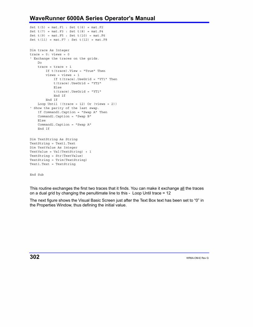
WaveRunner 6000A Series Operator's Manual
302 WR6A-OM-E Rev G
Set t(5) = mat.F1 : Set t(6) = mat.F2 Set t(7) = mat.F3 : Set t(8) = mat.F4 Set t(9) = mat.F5 : Set t(10) = mat.F6 Set t(11) = mat.F7 : Set t(12) = mat.F8 Dim trace As Integer trace = 0: views = 0 ' Exchange the traces on the grids. Do trace = trace + 1 If t(trace).View = "True" Then views = views + 1 If t(trace).UseGrid = "YT1" Then t(trace).UseGrid = "YT2" Else t(trace).UseGrid = "YT1" End If End If Loop Until ((trace = 12) Or (views = 2)) ' Show the parity of the last swap. If Command1.Caption = "Swap A" Then Command1.Caption = "Swap B" Else Command1.Caption = "Swap A" End If Dim TextString As String TextString = Text1.Text Dim TextValue As Integer TextValue = Val(TextString) + 1 TextString = Str(TextValue) TextString = Trim(TextString) Text1.Text = TextString End Sub
This routine exchanges the first two traces that it finds. You can make it exchange all the traces on a dual grid by changing the penultimate line to this - Loop Until trace = 12
The next figure shows the Visual Basic Screen just after the Text Box text has been set to “0” in the Properties Window, thus defining the initial value.

WR6A-OM-E Rev G 303
Here is the result after seven swaps. The counting method could be useful in any routine where numerous operations, such as triggers, have to be performed. In fact, the caption of the button could have been used to show the number of operations.
ActiveX offers a large range of standard controls, including list boxes for selection from a list, and picture boxes for drawing graphs and charts.
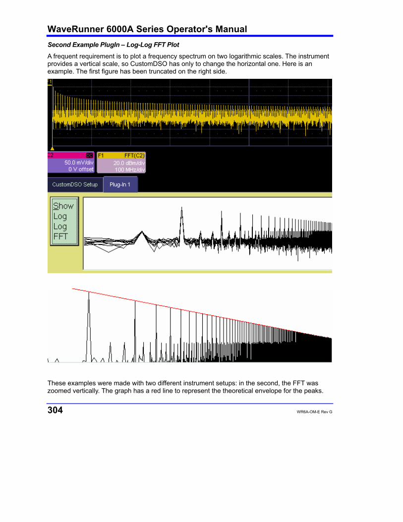
WaveRunner 6000A Series Operator's Manual
304 WR6A-OM-E Rev G
Second Example PlugIn – Log-Log FFT Plot
A frequent requirement is to plot a frequency spectrum on two logarithmic scales. The instrument provides a vertical scale, so CustomDSO has only to change the horizontal one. Here is an example. The first figure has been truncated on the right side.
These examples were made with two different instrument setups: in the second, the FFT was zoomed vertically. The graph has a red line to represent the theoretical envelope for the peaks.
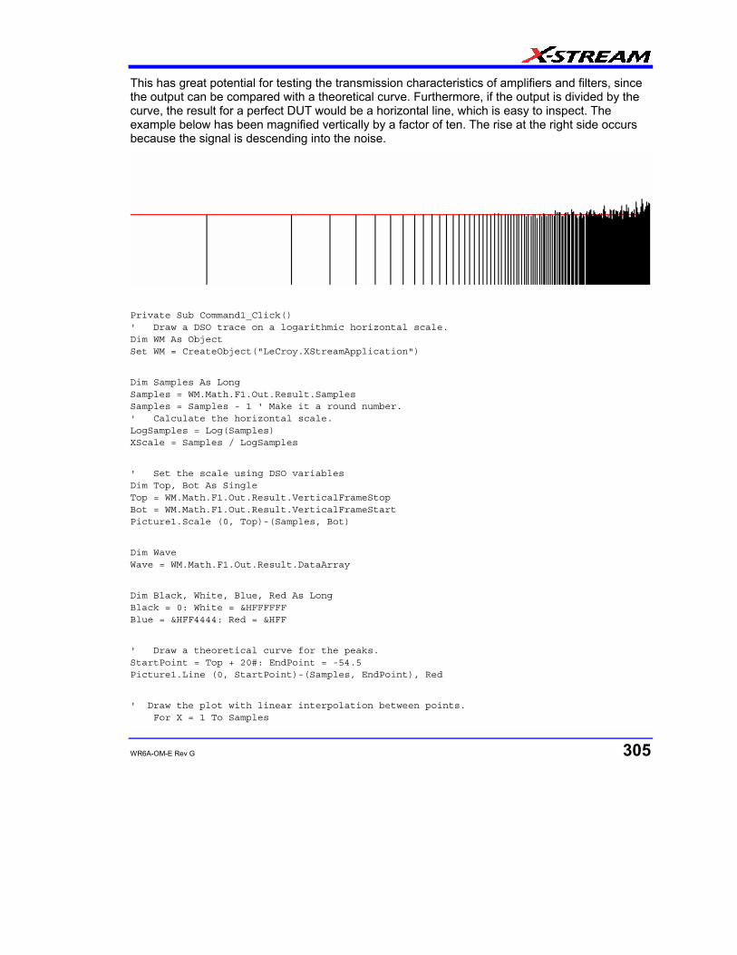
WR6A-OM-E Rev G 305
This has great potential for testing the transmission characteristics of amplifiers and filters, since the output can be compared with a theoretical curve. Furthermore, if the output is divided by the curve, the result for a perfect DUT would be a horizontal line, which is easy to inspect. The example below has been magnified vertically by a factor of ten. The rise at the right side occurs because the signal is descending into the noise.
Private Sub Command1_Click() ' Draw a DSO trace on a logarithmic horizontal scale. Dim WM As Object Set WM = CreateObject("LeCroy.XStreamApplication") Dim Samples As Long Samples = WM.Math.F1.Out.Result.Samples Samples = Samples - 1 ' Make it a round number. ' Calculate the horizontal scale. LogSamples = Log(Samples) XScale = Samples / LogSamples ' Set the scale using DSO variables Dim Top, Bot As Single Top = WM.Math.F1.Out.Result.VerticalFrameStop Bot = WM.Math.F1.Out.Result.VerticalFrameStart Picture1.Scale (0, Top)-(Samples, Bot) Dim Wave Wave = WM.Math.F1.Out.Result.DataArray Dim Black, White, Blue, Red As Long Black = 0: White = &HFFFFFF Blue = &HFF4444: Red = &HFF ' Draw a theoretical curve for the peaks. StartPoint = Top + 20#: EndPoint = -54.5 Picture1.Line (0, StartPoint)-(Samples, EndPoint), Red ' Draw the plot with linear interpolation between points. For X = 1 To Samples
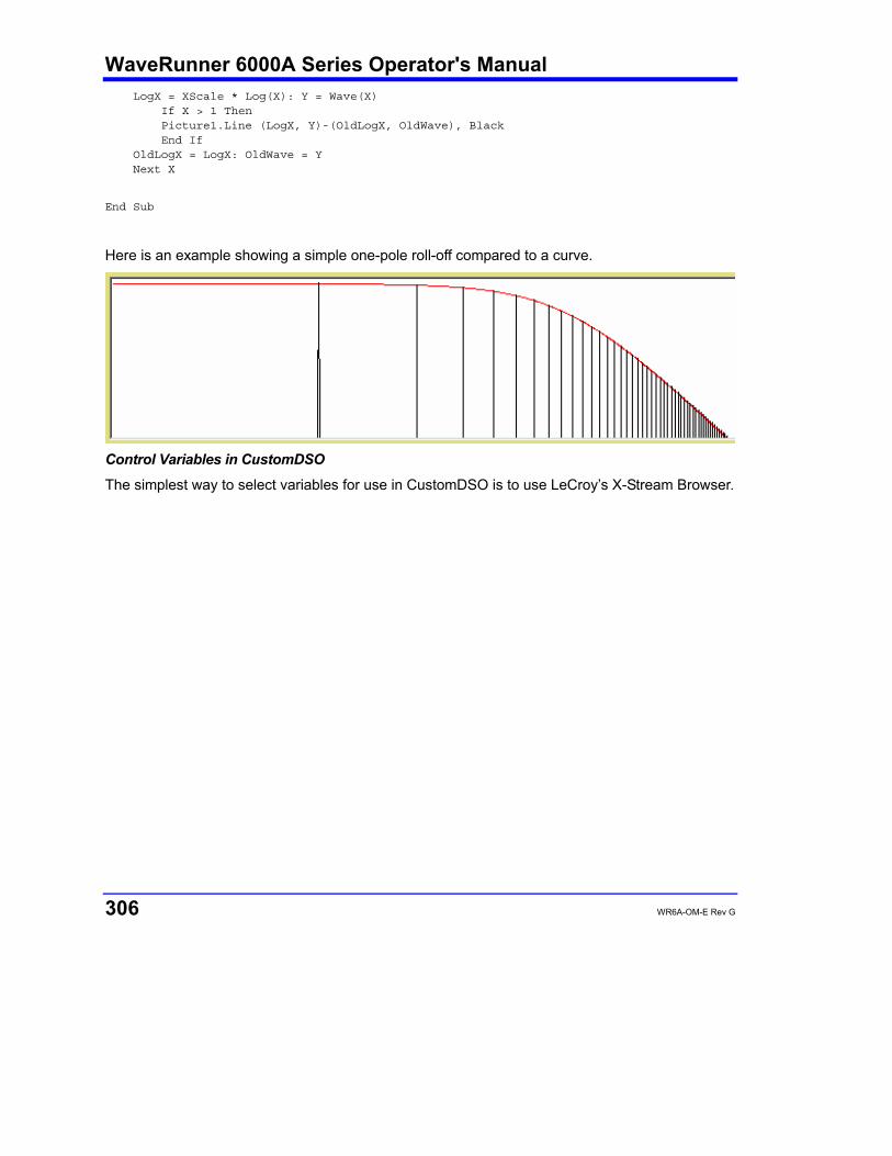
WaveRunner 6000A Series Operator's Manual
306 WR6A-OM-E Rev G
LogX = XScale * Log(X): Y = Wave(X) If X > 1 Then Picture1.Line (LogX, Y)-(OldLogX, OldWave), Black End If OldLogX = LogX: OldWave = Y Next X End Sub
Here is an example showing a simple one-pole roll-off compared to a curve.
Control Variables in CustomDSO
The simplest way to select variables for use in CustomDSO is to use LeCroy’s X-Stream Browser.
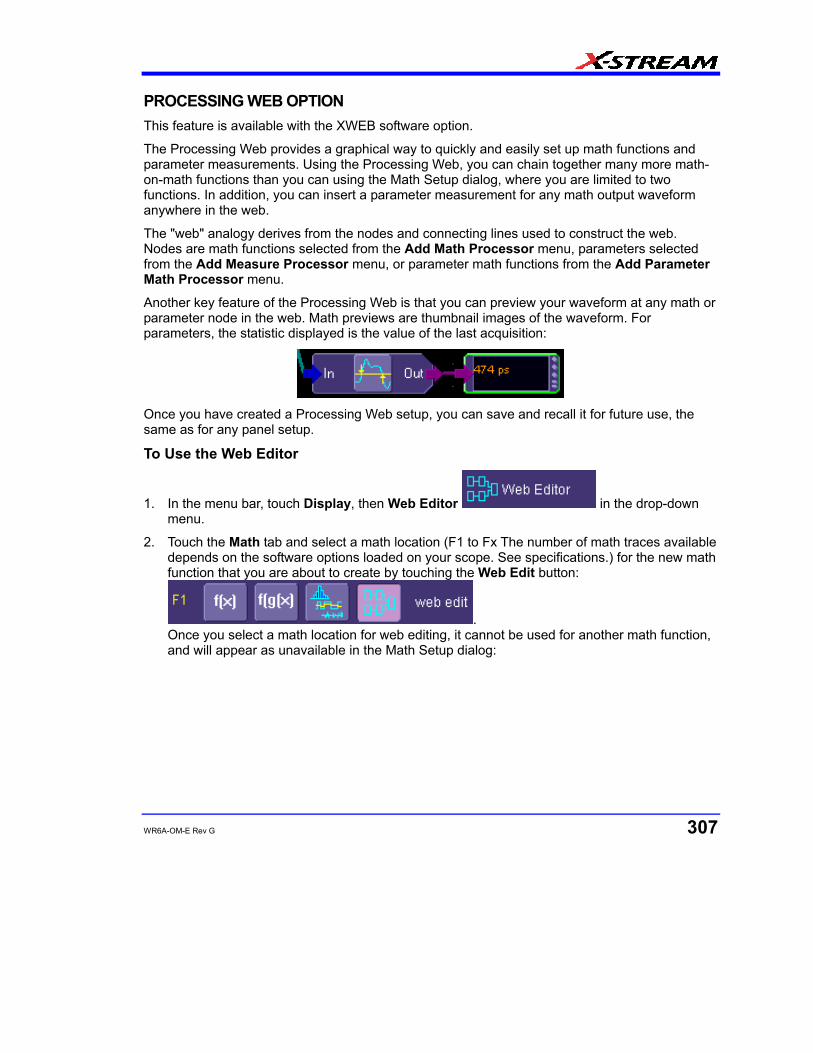
WR6A-OM-E Rev G 307
PROCESSING WEB OPTION This feature is available with the XWEB software option.
The Processing Web provides a graphical way to quickly and easily set up math functions and parameter measurements. Using the Processing Web, you can chain together many more math-on-math functions than you can using the Math Setup dialog, where you are limited to two functions. In addition, you can insert a parameter measurement for any math output waveform anywhere in the web.
The "web" analogy derives from the nodes and connecting lines used to construct the web. Nodes are math functions selected from the Add Math Processor menu, parameters selected from the Add Measure Processor menu, or parameter math functions from the Add Parameter Math Processor menu.
Another key feature of the Processing Web is that you can preview your waveform at any math or parameter node in the web. Math previews are thumbnail images of the waveform. For parameters, the statistic displayed is the value of the last acquisition:
Once you have created a Processing Web setup, you can save and recall it for future use, the same as for any panel setup.
To Use the Web Editor
1. In the menu bar, touch Display, then Web Editor in the drop-down menu.
2. Touch the Math tab and select a math location (F1 to Fx The number of math traces available depends on the software options loaded on your scope. See specifications.) for the new math function that you are about to create by touching the Web Edit button:
. Once you select a math location for web editing, it cannot be used for another math function, and will appear as unavailable in the Math Setup dialog:
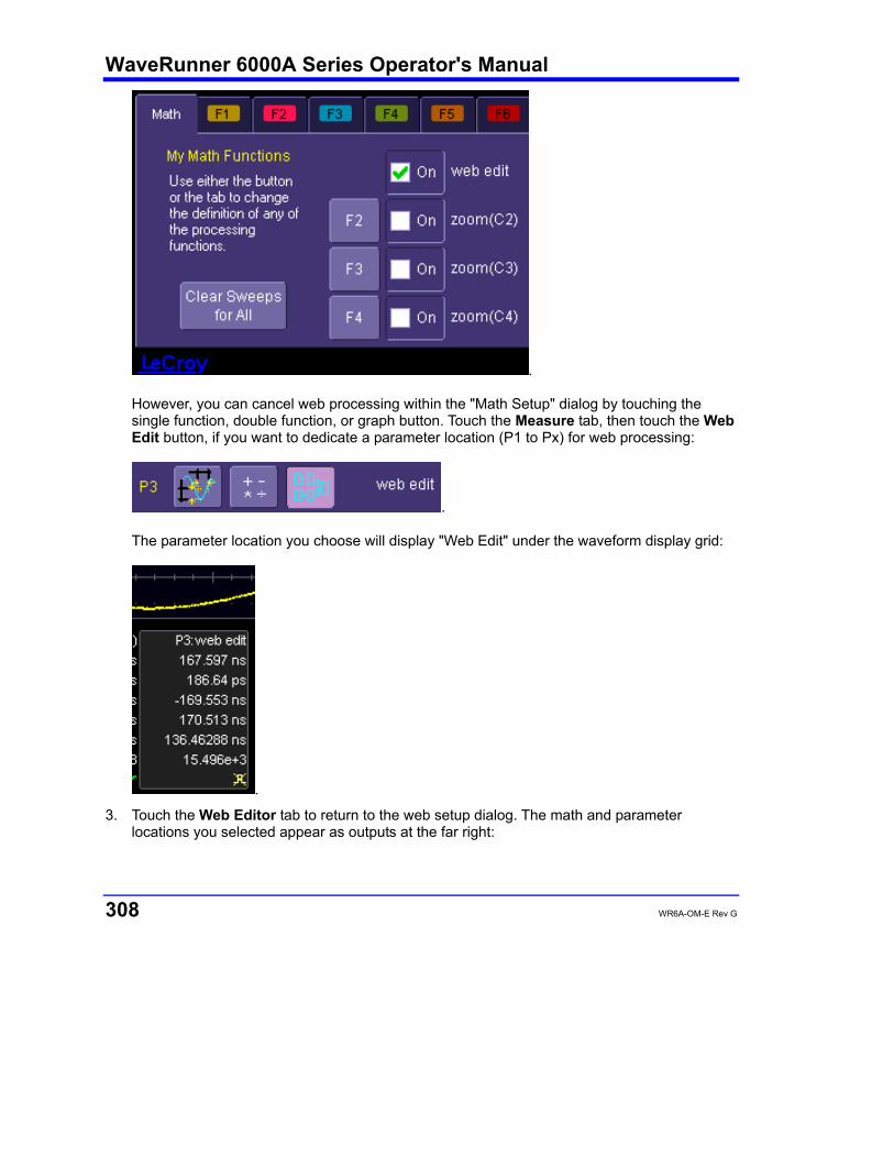
WaveRunner 6000A Series Operator's Manual
308 WR6A-OM-E Rev G
. However, you can cancel web processing within the "Math Setup" dialog by touching the single function, double function, or graph button. Touch the Measure tab, then touch the Web Edit button, if you want to dedicate a parameter location (P1 to Px) for web processing:
. The parameter location you choose will display "Web Edit" under the waveform display grid:
.
3. Touch the Web Editor tab to return to the web setup dialog. The math and parameter locations you selected appear as outputs at the far right:

WR6A-OM-E Rev G 309
. You may have to scroll up or down to see it.
4. Touch the Add Math button and select a math function from the Add Math Processor menu. The math function icon will appear on the web setup field:
. Touch and drag the icon to the desired location.
5. If you are using channel inputs, touch the arrow of a channel input icon:
. Then drag a line from the channel to the input of the math function icon. If your math function is a dual input function (such as ratio), select a second input and drag another line to the second math input. If you are using a memory location:
(M1 to M4) as an input, drag a line to the math function in the same way as for channel inputs.
Note: You can use a combination of channel input and memory input to your math function.
6. Touch the output arrow of the math function icon and drag a line to the Fx output on the right-hand side of the setup field. Your math function is complete.
Adding Parameters
Add parameter measurements in the same way as for math functions. Parameters can be connected to any math function in the web.
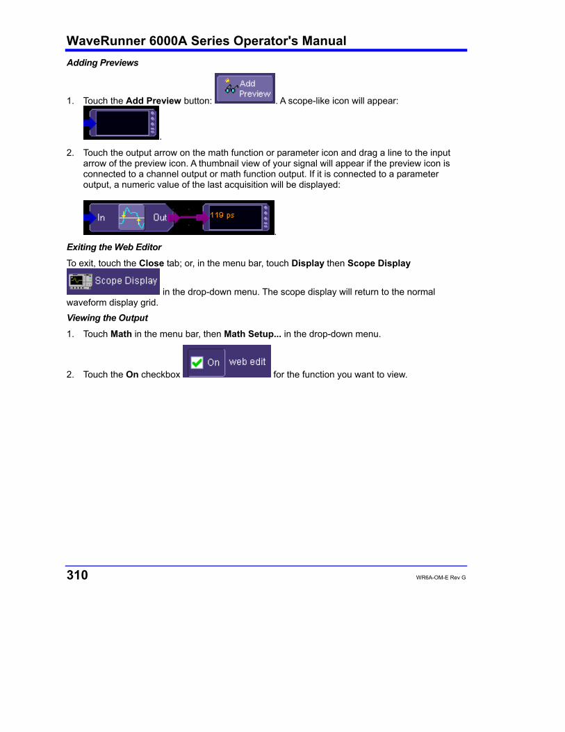
WaveRunner 6000A Series Operator's Manual
310 WR6A-OM-E Rev G
Adding Previews
1. Touch the Add Preview button: . A scope-like icon will appear:
.
2. Touch the output arrow on the math function or parameter icon and drag a line to the input arrow of the preview icon. A thumbnail view of your signal will appear if the preview icon is connected to a channel output or math function output. If it is connected to a parameter output, a numeric value of the last acquisition will be displayed:
. Exiting the Web Editor
To exit, touch the Close tab; or, in the menu bar, touch Display then Scope Display
in the drop-down menu. The scope display will return to the normal waveform display grid. Viewing the Output
1. Touch Math in the menu bar, then Math Setup... in the drop-down menu.
2. Touch the On checkbox for the function you want to view.
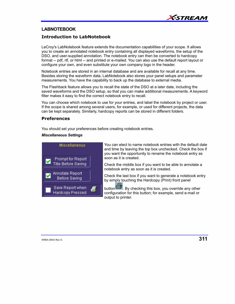
WR6A-OM-E Rev G 311
LABNOTEBOOK Introduction to LabNotebook
LeCroy's LabNotebook feature extends the documentation capabilities of your scope. It allows you to create an annotated notebook entry containing all displayed waveforms, the setup of the DSO, and user-supplied annotation. The notebook entry can then be converted to hardcopy format -- pdf, rtf, or html -- and printed or e-mailed. You can also use the default report layout or configure your own, and even substitute your own company logo in the header.
Notebook entries are stored in an internal database and are available for recall at any time. Besides storing the waveform data, LabNotebook also stores your panel setups and parameter measurements. You have the capability to back up the database to external media.
The Flashback feature allows you to recall the state of the DSO at a later date, including the saved waveforms and the DSO setup, so that you can make additional measurements. A keyword filter makes it easy to find the correct notebook entry to recall.
You can choose which notebook to use for your entries, and label the notebook by project or user. If the scope is shared among several users, for example, or used for different projects, the data can be kept separately. Similarly, hardcopy reports can be stored in different folders.
Preferences
You should set your preferences before creating notebook entries. Miscellaneous Settings
You can elect to name notebook entries with the default date and time by leaving the top box unchecked. Check the box if you want the opportunity to rename the notebook entry as soon as it is created.
Check the middle box if you want to be able to annotate a notebook entry as soon as it is created.
Check the last box if you want to generate a notebook entry by simply touching the Hardcopy (Print) front panel
button . By checking this box, you override any other configuration for this button; for example, send e-mail or output to printer.
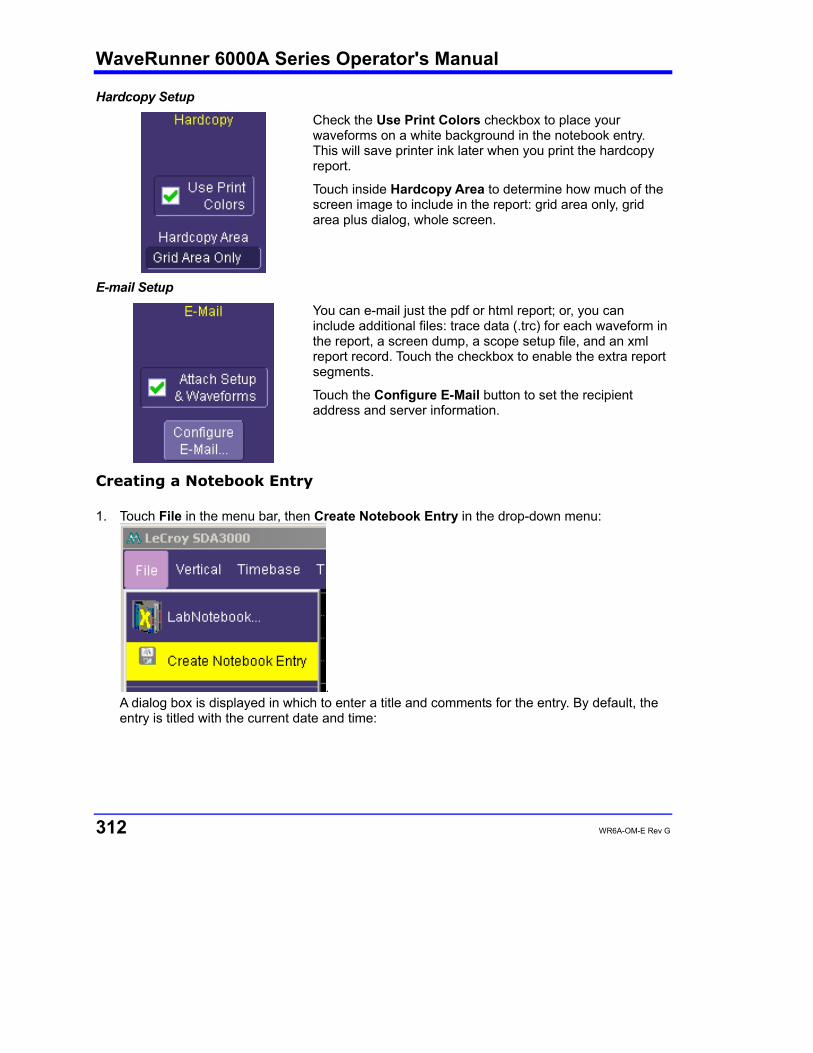
WaveRunner 6000A Series Operator's Manual
312 WR6A-OM-E Rev G
Hardcopy Setup
Check the Use Print Colors checkbox to place your waveforms on a white background in the notebook entry. This will save printer ink later when you print the hardcopy report.
Touch inside Hardcopy Area to determine how much of the screen image to include in the report: grid area only, grid area plus dialog, whole screen.
E-mail Setup
You can e-mail just the pdf or html report; or, you can include additional files: trace data (.trc) for each waveform in the report, a screen dump, a scope setup file, and an xml report record. Touch the checkbox to enable the extra report segments.
Touch the Configure E-Mail button to set the recipient address and server information.
Creating a Notebook Entry
1. Touch File in the menu bar, then Create Notebook Entry in the drop-down menu:
. A dialog box is displayed in which to enter a title and comments for the entry. By default, the entry is titled with the current date and time:

WR6A-OM-E Rev G 313
2. Touch inside the Title field and enter a title, using the pop-up keyboard. Then touch inside the Description field and enter a description, if desired, and touch Close.
The notebook entry will display your waveforms in "print colors," that is, on a white background to save printer ink, if you selected that option in notebook Preferences. Otherwise, the waveforms will appear on a black background. A drawing toolbar appears at top:
The pen tool enables you to write or draw in freehand. You can use a mouse, or a stylus to do this using the touch screen. Once you click off, you can drag your note anywhere on your waveform.
The circle tool enables you to create a circle around a waveform feature that you want to point out. Once you click off, the circle is drawn and you can drag it anywhere on the screen.
The arrow tool enables you to draw lines with arrowheads for callouts. You can rotate these lines through 360 degrees and drag them to any location on the screen.
The text tool enables you to enter text callouts on your report. When you touch this tool, a dialog box opens in which to enter text by means of a pop-up keyboard:

WaveRunner 6000A Series Operator's Manual
314 WR6A-OM-E Rev G
After you touch Close, your text will appear on the display as a draggable object.
These are the three default colors that you can select for shapes, lines, and text. To use additional colors, touch More.

WR6A-OM-E Rev G 315
When you touch More, a Custom box opens with the default color yellow displayed. Touch the yellow button to open the full color palette:
When you have chosen a custom color, touch Add to Custom Colors; the color will appear in the Custom Colors palette:
Then touch the color to enable it, and touch OK. The next object that you create will be in that color.
If you want to erase a drawing object, touch it to select it, then touch Erase Selected.
Touch Erase All to erase all drawn objects and text.
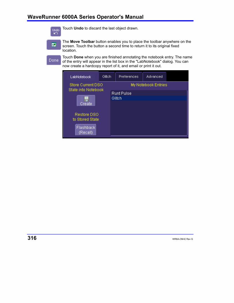
WaveRunner 6000A Series Operator's Manual
316 WR6A-OM-E Rev G
Touch Undo to discard the last object drawn.
The Move Toolbar button enables you to place the toolbar anywhere on the screen. Touch the button a second time to return it to its original fixed location.
Touch Done when you are finished annotating the notebook entry. The name of the entry will appear in the list box in the "LabNotebook" dialog. You can now create a hardcopy report of it, and email or print it out.
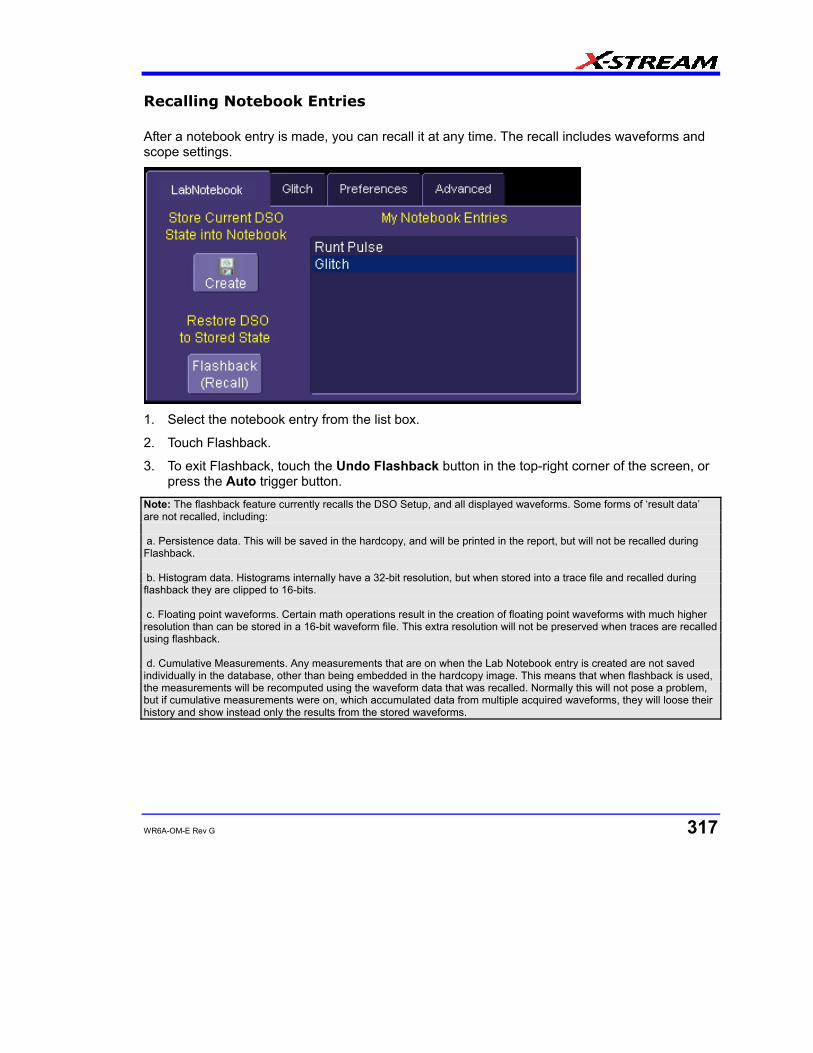
WR6A-OM-E Rev G 317
Recalling Notebook Entries
After a notebook entry is made, you can recall it at any time. The recall includes waveforms and scope settings.
1. Select the notebook entry from the list box.
2. Touch Flashback.
3. To exit Flashback, touch the Undo Flashback button in the top-right corner of the screen, or press the Auto trigger button.
Note: The flashback feature currently recalls the DSO Setup, and all displayed waveforms. Some forms of ‘result data’ are not recalled, including: a. Persistence data. This will be saved in the hardcopy, and will be printed in the report, but will not be recalled during Flashback. b. Histogram data. Histograms internally have a 32-bit resolution, but when stored into a trace file and recalled during flashback they are clipped to 16-bits. c. Floating point waveforms. Certain math operations result in the creation of floating point waveforms with much higher resolution than can be stored in a 16-bit waveform file. This extra resolution will not be preserved when traces are recalled using flashback. d. Cumulative Measurements. Any measurements that are on when the Lab Notebook entry is created are not saved individually in the database, other than being embedded in the hardcopy image. This means that when flashback is used, the measurements will be recomputed using the waveform data that was recalled. Normally this will not pose a problem, but if cumulative measurements were on, which accumulated data from multiple acquired waveforms, they will loose their history and show instead only the results from the stored waveforms.
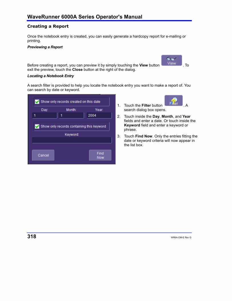
WaveRunner 6000A Series Operator's Manual
318 WR6A-OM-E Rev G
Creating a Report
Once the notebook entry is created, you can easily generate a hardcopy report for e-mailing or printing. Previewing a Report
Before creating a report, you can preview it by simply touching the View button . To exit the preview, touch the Close button at the right of the dialog. Locating a Notebook Entry
A search filter is provided to help you locate the notebook entry you want to make a report of. You can search by date or keyword.
1. Touch the Filter button . A search dialog box opens.
2. Touch inside the Day, Month, and Year fields and enter a date. Or touch inside the Keyword field and enter a keyword or phrase.
3. Touch Find Now. Only the entries fitting the date or keyword criteria will now appear in the list box.

WR6A-OM-E Rev G 319
Creating the Report
1. Select a notebook entry in the list box
.
2. Touch inside the Format field and select a report format from the pop-up menu
3. Touch the Create Report button.
4. A dialog box opens in which to name the report and select a folder to contain the report. Touch inside the File name field and enter a name using the pop-up keyboard.
5. If you want to e-mail or print the data to a network printer, touch More Actions, then the Print or E-Mail button. If you select Print, a Windows dialog box will open for you to select a printer and set options. If you select E-Mail, the report will be sent immediately to the e-mail address configured in Utilities Preferences.
Formatting the Report
LeCroy provides a default report format (template); however, you can use your own format, including company logo.
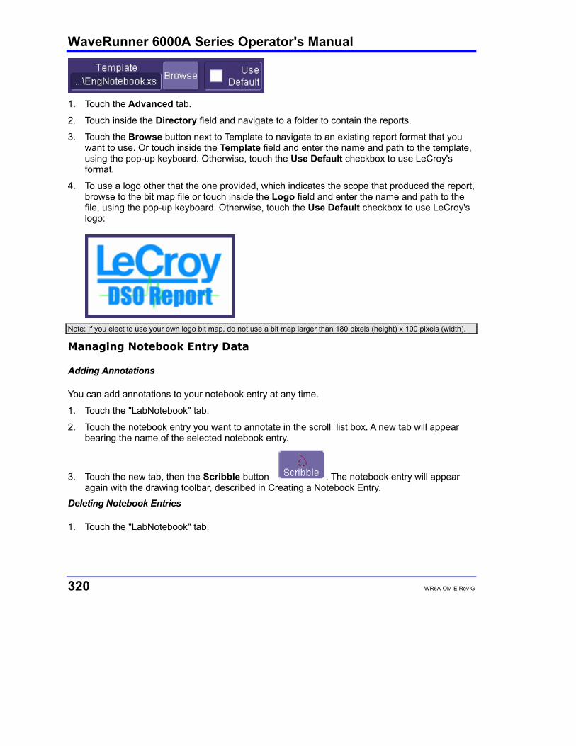
WaveRunner 6000A Series Operator's Manual
320 WR6A-OM-E Rev G
1. Touch the Advanced tab.
2. Touch inside the Directory field and navigate to a folder to contain the reports.
3. Touch the Browse button next to Template to navigate to an existing report format that you want to use. Or touch inside the Template field and enter the name and path to the template, using the pop-up keyboard. Otherwise, touch the Use Default checkbox to use LeCroy's format.
4. To use a logo other that the one provided, which indicates the scope that produced the report, browse to the bit map file or touch inside the Logo field and enter the name and path to the file, using the pop-up keyboard. Otherwise, touch the Use Default checkbox to use LeCroy's logo:
Note: If you elect to use your own logo bit map, do not use a bit map larger than 180 pixels (height) x 100 pixels (width).
Managing Notebook Entry Data
Adding Annotations
You can add annotations to your notebook entry at any time.
1. Touch the "LabNotebook" tab.
2. Touch the notebook entry you want to annotate in the scroll list box. A new tab will appear bearing the name of the selected notebook entry.
3. Touch the new tab, then the Scribble button . The notebook entry will appear again with the drawing toolbar, described in Creating a Notebook Entry.
Deleting Notebook Entries
1. Touch the "LabNotebook" tab.
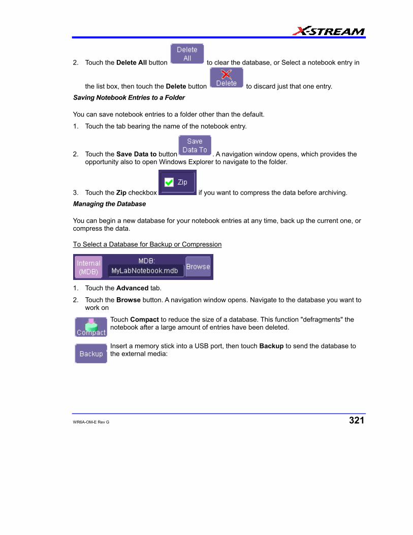
WR6A-OM-E Rev G 321
2. Touch the Delete All button to clear the database, or Select a notebook entry in
the list box, then touch the Delete button to discard just that one entry. Saving Notebook Entries to a Folder
You can save notebook entries to a folder other than the default.
1. Touch the tab bearing the name of the notebook entry.
2. Touch the Save Data to button . A navigation window opens, which provides the opportunity also to open Windows Explorer to navigate to the folder.
3. Touch the Zip checkbox if you want to compress the data before archiving. Managing the Database
You can begin a new database for your notebook entries at any time, back up the current one, or compress the data.
To Select a Database for Backup or Compression
1. Touch the Advanced tab.
2. Touch the Browse button. A navigation window opens. Navigate to the database you want to work on
Touch Compact to reduce the size of a database. This function "defragments" the notebook after a large amount of entries have been deleted.
Insert a memory stick into a USB port, then touch Backup to send the database to the external media:

WaveRunner 6000A Series Operator's Manual
322 WR6A-OM-E Rev G
To Start a New Database
Touch the Start New button. The name of the notebook database will be incremented by 1:
§ § §