Multiple Sequence Alignment

Evolution at the DNA level

…ACGGTGCAGTTACCA…

…AC----CAGTCCACCA…

Mutation

SEQUENCE EDITS

REARRANGEMENTS

Deletion

InversionTranslocationDuplication

All Homologous Sequences Coalesce

Y-chromosome coalescence

http://webvision.umh.es/webvision/Evolution.%20PART%20II.html

Orthology and Paralogy

HB HumanHB Human

WB WormWB Worm

HA1 HumanHA1 Human

HA2 HumanHA2 Human

YeastYeast

WA WormWA Worm

Orthologs:Derived by speciation

Paralogs:Everything else

Orthology, Paralogy, Inparalogs, Outparalogs

Phylogenetic Trees

• Nodes: species

• Edges: time of independent evolution

• Edge length represents evolution time

AKA genetic distance

Not necessarily chronological time

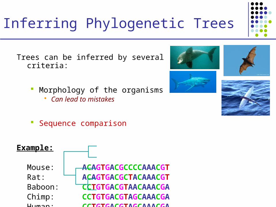
Inferring Phylogenetic Trees

Trees can be inferred by several criteria:

Morphology of the organisms• Can lead to mistakes

Sequence comparison

Example:

Mouse: ACAGTGACGCCCCAAACGTRat:ACAGTGACGCTACAAACGTBaboon:CCTGTGACGTAACAAACGAChimp: CCTGTGACGTAGCAAACGAHuman: CCTGTGACGTAGCAAACGA

Distance Between Two Sequences

Basic principle:• Distance proportional to degree of independent sequence evolution

Given sequences xi, xj,

dij = distance between the two sequences

One possible definition:

dij = fraction f of sites u where xi[u] xj[u]

Better scores are derived by modeling evolution as a continuous change process

Molecular Evolution

Modeling sequence substitution:

Consider what happens at a position for time Δt,

• P(t) = vector of probabilities of {A,C,G,T} at time t

• Given an alignment between two sequences, we can estimate P(t)

(Simplistic) Count non-match positions in the alignment

How do we estimate t from that information?

A

C

Δt ~= 0

Molecular Evolution

Modeling sequence substitution:

Consider what happens at a position for time Δt,

• P(t) = vector of probabilities of {A,C,G,T} at time t

• μAC = rate of transition from A to C per unit time

• μA = μAC + μAG + μAT rate of transition out of A

• pA(t+Δt) = pA(t) – pA(t) μA Δt + pC(t) μCA Δt + pG(t) μGA Δt + pT(t) μTA Δt

A

C

Δt ~= 0

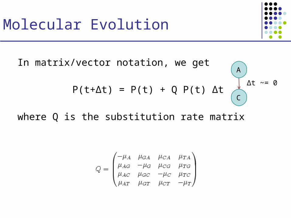
Molecular Evolution

In matrix/vector notation, we get

P(t+Δt) = P(t) + Q P(t) Δt

where Q is the substitution rate matrix

A

C

Δt ~= 0

Molecular Evolution

• This is a differential equation:

P’(t) = Q P(t)

• Q => prob. distribution over {A,C,G,T} at each position, stationary (equilibrium) frequencies πA, πC, πG, πT

• Each Q is an evolutionary model Some work better than others

A

C

Δt ~= 0

Evolutionary Models

• Jukes-Cantor

• Kimura

• Felsenstein

• HKY

Estimating Distances

• Solve the differential equation and compute expected evolutionary time given sequences

P’(t) = Q P(t)

Jukes-Cantor:

Let PAA(t) = PCC(t) = PCC(t) = PCC(t) = r

PAC(t) = … = PTG(t) = s

Then,

r’(t) = - ¾ r(t) m + ¾ s(t) ms’(t) = - ¼ s(t) m + ¼ r(t) m

Which is satisfied by

r(t) = ¼ (1 + 3e-mt)

s(t) = ¼ (1 - e-mt)

Estimating Distances

• Solve the differential equation and compute expected evolutionary time given sequences

P’(t) = Q P(t)

Jukes-Cantor:

Estimating Distances

Let p = probability a base is different between two sequences,

Solve to find t

• Jukes-Cantor r(t) = 1 – p = ¼ (1 + 3e-mt)

p = ¾ – ¾ e-mt

¾ – p = ¾ e-mt

1 – 4p/3 = e-mt

Therefore,

mt = - ln(1 – 4p/3)

Letting d = ¾ mt, denoting substitutions per site,

Estimating Distances

d: Branch length in terms of substitutions per site

• Jukes-Cantor

• Kimura

A simple clustering method for building tree

UPGMA (unweighted pair group method using arithmetic averages)Or the Average Linkage Method

Given two disjoint clusters Ci, Cj of sequences,

1dij = ––––––––– {p Ci, q Cj}dpq

|Ci| |Cj|

Claim that if Ck = Ci Cj, then distance to another cluster Cl is:

dil |Ci| + djl |Cj| dkl = ––––––––––––––

|Ci| + |Cj|

Algorithm: Average Linkage

Initialization:Assign each xi into its own cluster Ci

Define one leaf per sequence, height 0

Iteration:Find two clusters Ci, Cj s.t. dij is min

Let Ck = Ci Cj

Define node connecting Ci, Cj, and place it at height dij/2

Delete Ci, Cj

Termination:When two clusters i, j remain, place root at

height dij/2

1 4

3 2 5

1 4 2 3 5

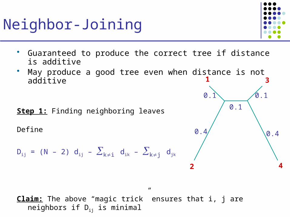
Neighbor-Joining

• Guaranteed to produce the correct tree if distance is additive• May produce a good tree even when distance is not additive

Step 1: Finding neighboring leaves

Define

Dij = (N – 2) dij – ki dik – kj djk

Claim: The above “magic trick” ensures that i, j are neighbors if Dij is minimal

1

2 4

3

0.1

0.1 0.1

0.4 0.4

Mammalian alignments

Genome Evolutionary Rate Profiling (GERP)

Rasmussen M D , Kellis M Genome Res. 2007;17:1932-1942

©2007 by Cold Spring Harbor Laboratory Press

Species Trees and Gene Trees

Evolutionary rates decoupled into gene-specific and species-specific components

Rasmussen M D , Kellis M Genome Res. 2007;17:1932-1942

©2007 by Cold Spring Harbor Laboratory Press

Evaluating gene-tree likelihood using learned rate distributions.

Rasmussen M D , Kellis M Genome Res. 2007;17:1932-1942

Multiple Sequence Alignments

Definition

Given N sequences x1, x2,…, xN: Insert gaps (-) in each sequence xi, such that

• All sequences have the same length L• Score of the global map is maximum

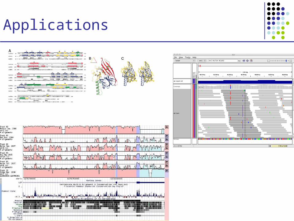
Applications

Scoring Function: Sum Of Pairs

Definition: Induced pairwise alignment

A pairwise alignment induced by the multiple alignment

Example:

x: AC-GCGG-C y: AC-GC-GAG z: GCCGC-GAG

Induces:

x: ACGCGG-C; x: AC-GCGG-C; y: AC-GCGAGy: ACGC-GAC; z: GCCGC-GAG; z: GCCGCGAG

Sum Of Pairs (cont’d)

• Heuristic way to incorporate evolution tree:

Human

Mouse

Chicken

• Weighted SOP:

S(m) = k<l wkl s(mk, ml)

Duck

A Profile Representation

• Given a multiple alignment M = m1…mn Replace each column mi with profile entry pi

• Frequency of each letter in • # gaps• Optional: # gap openings, extensions, closings

Can think of this as a “likelihood” of each letter in each position

- A G G C T A T C A C C T G T A G – C T A C C A - - - G C A G – C T A C C A - - - G C A G – C T A T C A C – G G C A G – C T A T C G C – G G

A 0 1 0 0 0 0 1 0 0 .8 0 0 0 0C .6 0 0 0 1 0 0 .4 1 0 .6 .2 0 0G 0 0 1 .2 0 0 0 0 0 .2 0 0 .4 1T .2 0 0 0 0 1 0 .6 0 0 0 0 .2 0- .2 0 0 .8 0 0 0 0 0 0 .4 .8 .4 0

Multiple Sequence Alignments

Algorithms

Multidimensional DP

Generalization of Needleman-Wunsh:

S(m) = i S(mi)

(sum of column scores)

F(i1,i2,…,iN): Optimal alignment up to (i1, …, iN)

F(i1,i2,…,iN)= max(all neighbors of cube)(F(nbr)+S(nbr))

• Example: in 3D (three sequences):

• 7 neighbors/cell

F(i,j,k) = max{ F(i – 1, j – 1, k – 1) + S(xi, xj, xk),

F(i – 1, j – 1, k ) + S(xi, xj, - ),F(i – 1, j , k – 1) + S(xi, -, xk),F(i – 1, j , k ) + S(xi, -, - ),F(i , j – 1, k – 1) + S( -, xj, xk),F(i , j – 1, k ) + S( -, xj, - ),F(i , j , k – 1) + S( -, -, xk) }

Multidimensional DP

Running Time:

1. Size of matrix: LN;

Where L = length of each sequence

N = number of sequences

2. Neighbors/cell: 2N – 1

Therefore………………………… O(2N LN)

Multidimensional DP

Running Time:

1. Size of matrix: LN;

Where L = length of each sequence

N = number of sequences

2. Neighbors/cell: 2N – 1

Therefore………………………… O(2N LN)

Multidimensional DP

Progressive Alignment

• When evolutionary tree is known:

Align closest first, in the order of the tree In each step, align two sequences x, y, or profiles px, py, to generate a new

alignment with associated profile presult

Weighted version: Tree edges have weights, proportional to the divergence in that edge New profile is a weighted average of two old profiles

x

w

y

z

pxy

pzw

pxyzw

Progressive Alignment

• When evolutionary tree is known:

Align closest first, in the order of the tree In each step, align two sequences x, y, or profiles px, py, to generate a new

alignment with associated profile presult

Weighted version: Tree edges have weights, proportional to the divergence in that edge New profile is a weighted average of two old profiles

x

w

y

z

Example

Profile: (A, C, G, T, -)px = (0.8, 0.2, 0, 0, 0)py = (0.6, 0, 0, 0, 0.4)

s(px, py) = 0.8*0.6*s(A, A) + 0.2*0.6*s(C, A) + 0.8*0.4*s(A, -) + 0.2*0.4*s(C, -)

Result: pxy = (0.7, 0.1, 0, 0, 0.2)

s(px, -) = 0.8*1.0*s(A, -) + 0.2*1.0*s(C, -)

Result: px- = (0.4, 0.1, 0, 0, 0.5)

Progressive Alignment

• When evolutionary tree is unknown:

Perform all pairwise alignments Define distance matrix D, where D(x, y) is a measure of evolutionary

distance, based on pairwise alignment Construct a tree (UPGMA / Neighbor Joining / Other methods) Align on the tree

x

w

y

z?

MUSCLE at a glance

1. Fast measurement of all pairwise distances between sequences • DDRAFT(x, y) defined in terms of # common k-mers (k~3) – O(N2 L logL) time

2. Build tree TDRAFT based on those distances, with UPGMA

3. Progressive alignment over TDRAFT, resulting in multiple alignment MDRAFT

4. Measure new Kimura-based distances D(x, y) based on MDRAFT

5. Build tree T based on D

6. Progressive alignment over T, to build M

7. Iterative refinement; for many rounds, do:• Tree Partitioning: Split M on one branch and realign the two resulting profiles• If new alignment M’ has better sum-of-pairs score than previous one, accept