0100297

7/28/2019 0100297

http://slidepdf.com/reader/full/0100297 1/4

EMPLOYING LAPLACIAN-GAUSSIAN DENSITIES FOR SPEECH ENHANCEMENT

Saeed Gazor

Department of Electrical and Computer Engineering, Queen’s University, Kingston, Ontario K7L 3N6, Canada

Abstract–A new efficient Speech Enhancement Algorithm (SEA)

is developed in this paper. A noisy speech is first decorrelated and

then the clean speech components are estimated from the decorre-

lated noisy speech samples. The distributions of clean speech and

noise are assumed to be Laplacian and Gaussian, respectively. The

clean speech components are estimated either by Maximum Likeli-

hood (ML) or Minimum-Mean-Square-Error (MMSE) estimators.

These estimators require some statistical parameters that are adap-

tively extracted by the ML approach during the active speech or

silence intervals, respectively. A Voice Activity Detector (VAD) is

employed to detect whether the speech is active or not. The simu-

lation results show that this SEA performs as well as a recent high

efficiency SEA that employs the Wiener filter. The complexity of

this algorithm is very low compared with existing SEAs.

1. INTRODUCTION

Most of Speech Enhancement (SE) research has focused on re-

moving the corrupting noise. Usually it is assumed that speech is

degraded by additive noise which is independent of clean speech.

In early implementations, spectral subtraction approach was widely

used. This approach estimates the Power Spectral Density (PSD)

of a clean signal by subtracting the short-time PSD of the noise

from the PSD of the noisy signal [1]. The Wiener and Kalman

filters have been used for SE [3, 4]. The noisy speech is used to

estimate an “optimum” filter adaptively, under the assumption that

speech and noise are Gaussian, independent and have zero mean.

Recently a signal subspace speech enhancement framework has

been developed (see [5–7] and references therein). This signal

subspace SE system decomposes the noisy signal into uncorrelated

components by applying the Karhunen-Loeve Transform (KLT).

The recent statistical modelling presented in [8] concludes that

the clean speech components, in decorrelated domains (e.g., in the

KLT and the DCT domains) as random variables have Laplacian

distributions, and noise components are accurately modelled by

Gaussian distributions. Therefore, the speech decorrelated com-

ponents could be accurately modelled as a multivariate Laplacian

random vector, while for noise a multivariate Gaussian model is

accurate. Based on these assumptions, we design a Bayesian SE

system to estimate the clean speech signal components.

This paper is organized as follows. Section 2 reviews the basic

principle of the decorrelation of speech signals. Section 3 provides

the statistical modelling that will be used in this paper. A SEA isproposed in Section 4. The performance evaluation and conclusion

are summarized in Section 5. Section 6 is the conclusion.

2. DECORRELATION OF SPEECH SIGNALS

Let x(t) be the clean speech and the vector of samples of x(t) be

denoted by X (m) = [x(m), x(m − 1), · · · , x(m − K + 1)]T

where (.)T is the transpose operation. Also, let Y (m) = X (m) +N (m) denote the corresponding K -dimensional vector of noisy

speech, assuming that the noise vector N (m) is additive. Ap-

plying a linear transformation to the noisy the speech signal we

may approximately assume that signal components are uncorre-

lated in the transformed domain. Since the correlation between

speech signals is commonly rather high, a speech data vector can

be represented with a small error by a small number of compo-

nents [7]. In this paper, the speech signals are transformed into

uncorrelated components by using the DCT or the AKLT [6]. It

can be easily seen that vi(m) = si(m) + ui(m), where vi(m),

si(m) and ui(m) are transformed components of Y (m), X (m)and N (m), respectively. In order to develop our SEA, we further

assume that the uncorrelated components, i.e., {si, ui}K

i=1, are in-dependent [8]. This assumption is not required if random variables

uncorrelated are Gaussian variables and are uncorrelated. As the

KLT is complex to compute, harmonic transforms such as Discrete

Cosine Transform (DCT) and Discrete Fourier Transform (DFT)

are used as suboptimal alternatives. Another motivation for using

these transforms instead of the AKLT is to avoid the subspace vari-

ations and errors of the AKLT [6]. Among the DCT and DFT, the

DCT is cheaper and reduces better the correlation of the signal and

compacts the energy of a signal block into some of the coefficients.

3. STATISTICAL MODELLING

The noise samples can be separated during silence intervals us-

ing a VAD. For a Gaussian noise component ui(m) with variance

σ2i (m), we have: f ui,m(ui(m)) =

exp(− u2i (m)

2σ2i(m)

)

√ 2πσ2

i(m)

. If the sam-

ples {ui(i)}mi=m−M N +1are iid, the ML estimate of σ2

i is σ2i =

1M N

m

t=m−M N +1|ui(t)|2. A lower-complexity estimator is

σ2i (m) = β N σ2

i (m − 1) + (1 − β N )|ui(m)|2, (1)

where β N is chosen to let the time constant of the above filter be

0.5 second, assuming that the variation of the noise spectrum is

negligible over a time interval of 0.5 second.

Assuming that the components of the clean speech in the decor-

related domains, {si(m)}Ki=1, follow zero-mean Laplacian are un-

correlated, we have f si,m(si(m)) = 12ai(m)e

−|si(m)|ai(m) , where ai(m)

is the Laplacian factor [8]. Similarly, the ML estimate of the

Laplacian Factor ai yields ai(m) = 1M S

mt=m−M S+1

|si(t)|. Sim-

ilarly, we use the following low-complexity substitute:

ai(m) = β S ai(m − 1) + (1 − β S) |si(m)| . (2)

In our simulations, β S is chosen to let the time constant of the

above adaptive process be 10msec, because the speech signal can

I - 2970-7803-8484-9/04/$20.00 ©2004 IEEE ICASSP 2004

«

http://0100293.pdf/

7/28/2019 0100297


-

6s

−σ2

a

σ2

aML→

MMSE→

v

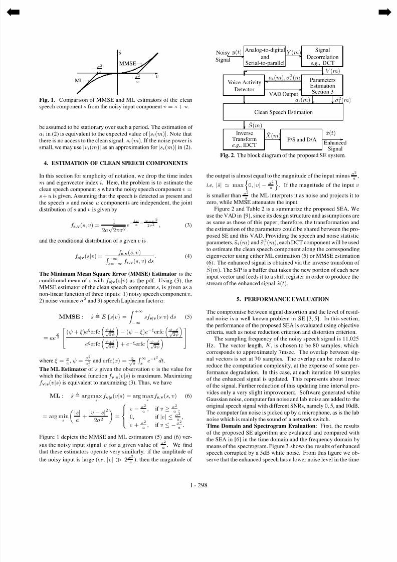
Fig. 1. Comparison of MMSE and ML estimators of the cleanspeech component s from the noisy input component v = s + u.

be assumed to be stationary over such a period. The estimation of

ai in (2) is equivalent to the expected value of |si(m)|. Note that

there is no access to the clean signal, si(m). If the noise power is

small, we may use |vi(m)| as an approximation for |si(m)| in (2).

4. ESTIMATION OF CLEAN SPEECH COMPONENTS

In this section for simplicity of notation, we drop the time index

m and eigenvector index i. Here, the problem is to estimate the

clean speech component s when the noisy speech component v =

s + u is given. Assuming that the speech is detected as present andthe speech s and noise u components are independent, the joint

distribution of s and v is given by

f s,v(s, v) =1

2a√

2πσ2e− |s|

a− |v−s|2

2σ2 , (3)

and the conditional distribution of s given v is

f s|v(s|v) =

f s,v(s, v) +∞s=−∞ f s,v(s, v) ds

. (4)

The Minimum Mean Square Error (MMSE) Estimator is the

conditional mean of s with f s|v(s|v) as the pdf. Using (3), the

MMSE estimator of the clean speech component s, is given as a

non-linear function of three inputs: 1) noisy speech component v,2) noise variance σ2 and 3) speech Laplacian factor a:

MMSE : s E {s|v} =

+∞−∞

sf s|v(s|v) ds (5)

= aeψ2

⎡⎣ (ψ + ξ)eξerfcψ+ξ√ 2ψ

− (ψ − ξ)e−ξerfc

ψ−ξ√ 2ψ

eξerfc

ψ+ξ√ 2ψ

+ e−ξerfc

ψ−ξ√ 2ψ

⎤⎦

where ξ = va

, ψ =σ2ia2i

and erfc(x) = 2√ π

∞x

e−t2

dt.

The ML Estimator of s given the observation v is the value for

which the likelihood function f v|s(v|s) is maximum. Maximizing

f v|s(v|s) is equivalent to maximizing (3). Thus, we have

ML : s argmaxs

f v|s(v|s) = arg maxs

f s,v(s, v) (6)

= arg mins

|s|a

+|v − s|2

2σ2

=

⎧⎪⎨⎪⎩v − σ2

a, if v ≥ σ2

a,

0, if |v| ≤ σ2

a,

v + σ2

a, if v ≤ −σ2

a.

Figure 1 depicts the MMSE and ML estimators (5) and (6) ver-

sus the noisy input signal v for a given value of σ2

a. We find

that these estimators operate very similarly; if the amplitude of

the noisy input is large (i.e, |v| 2σ2

a), then the magnitude of

Noisy

Signal

Voice Activity

Detector

-Analog-to-digital

andSerial-to-parallel

y(t)

VAD Output

ai(m), σ2i (m)

Y (m) Signal

Decorrelatione.g., DCT

V (m)

ParametersEstimationSection 3

ai(m) ? σ2i (m) ?

-

-

?

?Clean Speech Estimation

?

?S (m)

P/S and D/A

x(t)-X (m)-

EnhancedSignal

InverseTransforme.g., IDCT

Fig. 2. The block diagram of the proposed SE system.

the output is almost equal to the magnitude of the input minus σ2

a,

i.e, |s| max

0, |v| − σ2

a

. If the magnitude of the input v

is smaller thanσ2

a the ML interprets it as noise and projects it tozero, while MMSE attenuates the input.

Figure 2 and Table 2 is a summarize the proposed SEA. We

use the VAD in [9], since its design structure and assumptions are

as same as those of this paper; therefore, the transformation and

the estimation of the parameters could be shared between the pro-

posed SE and this VAD. Providing the speech and noise statistic

parameters, ai(m) and σ2i (m), each DCT component will be used

to estimate the clean speech component along the corresponding

eigenvector using either ML estimation (5) or MMSE estimation

(6). The enhanced signal is obtained via the inverse transform of

S (m). The S/P is a buffer that takes the new portion of each new

input vector and feeds it to a shift register in order to produce the

stream of the enhanced signal x(t).

5. PERFORMANCE EVALUATION

The compromise between signal distortion and the level of resid-

ual noise is a well known problem in SE [3, 5]. In this section,

the performance of the proposed SEA is evaluated using objective

criteria, such as noise reduction criterion and distortion criterion.

The sampling frequency of the noisy speech signal is 11,025

Hz. The vector length, K , is chosen to be 80 samples, which

corresponds to approximately 7msec. The overlap between sig-

nal vectors is set at 70 samples. The overlap can be reduced to

reduce the computation complexity, at the expense of some per-

formance degradation. In this case, at each iteration 10 samples

of the enhanced signal is updated. This represents about 1msec

of the signal. Further reduction of this updating time interval pro-

vides only a very slight improvement. Software generated whiteGaussian noise, computer fan noise and lab noise are added to the

original speech signal with different SNRs, namely 0, 5, and 10dB.

The computer fan noise is picked up by a microphone, as is the lab

noise which is mainly the sound of a network switch.

Time Domain and Spectrogram Evaluation: First, the results

of the proposed SE algorithm are evaluated and compared with

the SEA in [6] in the time domain and the frequency domain by

means of the spectrogram. Figure 3 shows the results of enhanced

speech corrupted by a 5dB white noise. From this figure we ob-

serve that the enhanced speech has a lower noise level in the time

I - 298

¬

7/28/2019 0100297


Table 1. Summary of the soft VAD algorithm in [9]

Initialize: β S = 0.913, β N = 0.983, P 1|0 = 12

,For each time step m do: vi(m) = [dct{Y (m)}]

i,

For i= 1, 2,· · · , K , if P m|m−1 ≥ 0.5 do

ai(m) = β Sai(m − 1) + (1 − β S) |vi(m)|if else do σ2i (m) = β N σ2i (m − 1) + (1 − β N )u2i (m) end;

f 0i(m) =1

2πσ2i (m)

e− v2

i(m)

2σ2i(m)

f 1i(m) =eψi,m2

4ai(m)

eξi,merfc

ψi,m + ξi,m

2ψi,m

+

+e−ξi,merfc

ψi,m − ξi,m

2ψi,m

,

where ξi,m =vi(m)

ai(m), and ψi,m =

σ2i (m)

a2i (m)end;

L(m) =K

i=1f 1i(m)

f 0i(m)

P m|m = L(m)P m|m−1L(m)P m|m−1 +

1 − P m|m−1

,

P m+1|m = Π01

1 − P m|m

+ Π11P m|m.

end;

Table 2. The structure of the proposed SEA.

Initialization: di(0) = 0, β S = 0.913, β N = 0.983,β S and β N are chosen to let the time constants of filters to

be 10msec and 0.5sec, respectively.

For each time step m do

V (m) =[v1(m), v2(m), · · · , vK(m)]T ←dct{Y (m)}For i= 1, 2,· · · , K do

ai(m) ← from (2)

if speech is absent: σ2

i (m) ← from (1) end;MMSE: si(m) ← from (5),or ML: si(m) ← from (6)

end; end;X (m) ← idct{[s1(m), , · · · , sK(m)]}

domain, where the ML approach results in a lower residual noise

level. From the spectrograms in Figure 3 it can be seen also that

the background noise is very efficiently reduced, while the energy

of most of the speech components remained unchanged.

Figures 3 and 4 illustrate the results for a nonstationary, col-

ored lab noise. From our simulations and Figures 3, 3 and 4, we

conclude that the proposed methods perform very well for various

noise conditions such as for colored and/or nonstationary noises.

The estimation of ai has an important impact on the perfor-

mance of the proposed SEAs. To illustrate this impact, we esti-mate the Laplacian factor ai using the clean speech signal and call

this estimate as “best value” of ai. In Figure 5, noisy speech is

enhanced with these so-called best values. We will use the term

“best value” to refer to the SEA that processes the noisy speech

with these so-called best values, which theoretically provides the

“best” performance that can be achieved with this SE framework

under the Laplacian-Gaussian assumption. We can clearly see that

the residual noise level of this ideal case is much lower than the re-

sults from Figure 3. This illustrates the effectiveness of the SEA.

(a) Speech signal

0 2 4 6 8 1 0Ŧ1

0

1

(b) Noisy signal

0 2 4 6 8 1 0Ŧ1

0

1

(c) Enhanced signal (ML)

0 2 4 6 8 1 0Ŧ1

0

1

(d) Enhanced signal (MMSE)

0 2 4 6 8 1 0Ŧ1

0

1

(e) Enhanced signal using [6]

0 2 4 6 8 1 0Ŧ1

0

1

Time (sec)

(a) Speech signal

r e q u e n c y

0 2 4 6 80

1000

2000

3000

4000

5000

(b) Noisy signal

0 2 4 6 80

1000

2000

3000

4000

5000


0 2 4 6 80

1000

2000

3000

4000

5000


0 2 4 6 80

1000

2000

3000

4000

5000


0 2 4 6 80

1000

2000

3000

4000

5000

Time (sec)

Fig. 3. Enhanced speech corrupted by white Gaussian noise

(SNR=5dB), and corresponding spectrograms.

(a) Speech signal

0 2 4 6 8 10Ŧ1

0

1

(b) Noisy signal

0 2 4 6 8 10Ŧ1

0

1


0 2 4 6 8 10Ŧ1

0

1


0 2 4 6 8 10Ŧ1

0

1


0 2 4 6 8 10Ŧ1

0

1

Fig. 4. Enhanced speech corrupted by nonstationary colored lab

noise (SNR=5dB).

(a) Speech signal

0 2 4 6 8 10Ŧ1

0

1

(b) Noisy signal

0 2 4 6 8 10Ŧ1

0

1

Time (sec)


0 2 4 6 8 10Ŧ1

0

1


0 2 4 6 8 10Ŧ1

0

1

Fig. 5. SEA results with the “best value”, white noise, SNR=5dB.

I - 299

¬

7/28/2019 0100297


Table 3. Spectral Distortion between the clean signal and signals

enhanced using different SEAs for various noise conditions.

Noise Input Input Proposed SEA best value of ai SEA

Type SNR SD MMSE ML MMSE ML in [6]

White 0dB 5.85 5.67 5.78 5.41 5.68 5.70

Gaussian 5dB 4.84 4.58 4.67 4.27 4.73 4.59

Noise 10dB 3.78 3.53 3.57 3.40 3.75 3.53

Lab 0dB 5.98 5.58 5.52 5.01 5.53 5.52Noise 5dB 4.91 4.58 4.54 4.11 4.51 4.49

10dB 3.81 3.54 3.55 3.24 3.53 3.49

Computer 0dB 4.88 4.12 4.34 4.96 4.59 4.29

Fan 5dB 3.73 3.26 3.53 3.50 3.77 3.47

Noise 10dB 2.71 2.56 2.82 2.81 3.02 2.77

Spectral Distortion: We use Spectral Distortion (SD) as a crite-

rion for the performance of SEAs. The SD in decibels (dB) be-

tween two signals x(t) and y(t) with length N is defined by

SD(x(t); y(t))=1

4N

N 64

i=1255

k=020 |log10 |X p(k)| − log10 |Y p(k)||.

where X p(k) and Y p(k) are the kth FFT frequency components of

the pth frame of x(t)||x(t)|| and

y(t)||y(t)|| , respectively. Signals are di-

vided into frames of length 64 samples without overlapping. After

padding 192 zeros into each frame, the 256-point FFT is calcu-

lated. Table 3 presents SDs where the clean speech signal is com-

pared with the noisy input signal, two proposed enhanced signals

and the enhanced signal using the algorithm in [6]. In white and

lab noise conditions, the SD values for all these approaches are

better than the noisy speech. The result of the “best value” MMSE

approach is slightly better than those of the others. Only for the

fan noise in a high SNR condition does the SD result seem to be

unexpected. The reason is that the PSD of the fan noise has an

strong peak at a low frequency that results in a strong SD around

this frequency.

The Output SNR of the enhanced signal (or the noisy signal) y(t)

is defined by SNR = 10log10

N k=1 x

2(k)N k=1 (y(k)−x(k))2

. Table 4 com-

pares the enhanced signals using different approaches versus the

input SNR. As expected, the SNR performance of the “best value”

MMSE is the best (highest) in all noise conditions. The SNR im-

provement in the MMSE approach for high SNRs is higher than

that of other approaches.

6. CONCLUSION

An SEA is developed based on a Laplacian distribution for speech

and a Gaussian distribution for additive noise signals. The en-

hancement is performed in a decorrelated domain. Each compo-

nent is estimated from the corresponding noisy speech component

by applying a non-linear memoryless filter. The speech signal is

decomposed into uncorrelated components by the DCT or by the

adaptive KLT. It is assumd that the speech is stationary within 20-

40msec and the noise is stationary over a longer period of about

0.5sec. The proposed SEAs are based on the MMSE and the ML

approaches, respectively. The speech is then synthesized by the

IDCT or IKLT. Overall, proposed SEAs effectively reduce the ad-

ditive noise. At the same time, the proposed SEAs produce a lower

level of distortion in the enhanced speech when compared with the

Table 4. Comparison of SNR (in dB) of enhanced signals for var-

ious noise conditions.Noise Input Proposed SEA best value SEA SEA

Type SNR MMSE ML MMSE ML in [6]

White 0dB 4.30 4.87 6.05 5.38 5.22

Gaussian 5dB 8.26 8.51 9.24 8.67 8.72

Noise 10dB 12.47 12.47 12.87 12.32 12.57

Lab 0dB 4.26 5.10 6.49 5.73 5.40Noise 5dB 8.27 8.64 9.45 8.64 8.78

10dB 12.33 12.32 12.84 11.99 12.37

Computer 0dB 5.74 5.90 6.48 6.15 6.04

Fan 5dB 9.87 9.82 10.26 9.84 9.94

Noise 10dB 13.46 13.29 13.57 13.16 13.37

method in [6] that uses a complex Adaptive KLT. The comparison

of results with the method in [6] shows that the proposed SEAs

provide a better (or similar) performance. The performance cri-

teria of the proposed SEAs give similar results. The fact that the

SEAs with “best value” outperformed all the others, indicates that

the new proposed framework for SE could be further improved.

The computational complexity of the proposed SEAs is very

low compared with the existing algorithms because of the use of fast DCT. In fact, most of the computationally complex parts are

the DCT and IDCT (the computational complexity the DCT and

IDCT is of the order of K log2(K ), where K is the size of the

vectors). All our simulations and listening evaluations confirm that

the proposed methods are very useful for SE.

7. REFERENCES

[1] Y. Ephraim and D. Malah, “Speech Enhancement Using aMinimum Mean-Square Error Short-Time Spectral AmplitudeEstimator,” IEEE Trans. Acoustics, Speech and Signal Pro-cessing, vol. 32, no. 6, pp. 1109-1121, Dec. 1984.

[2] S. M. McOlash, R. J. Niederjohn, and J. A. Heinen, “A Spec-tral Subtraction Method for the Enhancement of Speech Cor-

rupted by Nonwhite, Nonstationary Noise,” Proc. of IEEE Int.Conf. on Industrial Electronics, Control, and Instrumentation,vol. 2, pp. 872-877, 1995.

[3] I. Y. Soon and S. N. Koh, “Low Distortion Speech Enhance-ment,” IEE Proceedings-Vision, Image and Speech Process-ing, vol. 147, no. 3, pp. 247-253, June 2000.

[4] Z. Goh, K.-C. Tan, and B. T. G. Tan, “Kalman-FilteringSpeech Enhancement Method Based on a Voiced-unvoicedSpeech Model,” IEEE Transactions on Speech and Audio Pro-cessing, vol. 7, no. 5 , pp. 510-524, Sept. 1999.

[5] U. Mittal and N. Phamdo, “Signal/Noise KLT Based Ap-proach for Enhancing Speech Degraded by Colored Noise,”

IEEE Trans. Speech and Audio Processing, vol. 8, no. 2 , pp.159-167, March 2000.

[6] A. Rezayee and S. Gazor, “An Adaptive KLT Approach forSpeech Enhancement,” IEEE Trans. Speech and Audio Pro-

cessing, vol. 9, no. 2, pp. 87-95, Feb. 2001.[7] Y. Ephraim and H. L. Van Trees, “A Signal Subspace Ap-proach for Speech Enhancement,” IEEE Trans. Speech and

Audio Processing, vol. 3, no. 4, pp. 251-266, July, 1995.

[8] S. Gazor and W. Zhang, “Speech Probability Distribution”, IEEE, Signal Processing Letters, vol. 10, no. 7, pp. 204-207,July 2003.

[9] S. Gazor and W. Zhang “A soft voice activity detector basedon a laplacian-gaussian model”, IEEE Transactions on Speechand Audio Processing, vol. 11, no. 5, pp. 498-505, Sept. 2003.

I - 300

¬

0100297

Documents

Transcript of 0100297