00 A Fast and Scalable Multi-dimensional Multiple-choice Knapsack...
29
00 A Fast and Scalable Multi-dimensional Multiple-choice Knapsack Heuristic Hamid Shojaei 1∗ , Twan Basten 2,3 , Marc Geilen 2 , Azadeh Davoodi 1 1 Department of Electrical and Computer Engineering, University of Wisconsin - Madison 4621 Engineering Hall, 1415 Engineering Dr., Madison WI 53706 2 Department of Electrical Engineering, Eindhoven University of Technology PO Box 513, NL-5600 MB Eindhoven, The Netherlands 3 TNO-ESI PO Box 513, NL-5600 MB Eindhoven, The Netherlands ∗ Corresponding author, [email protected] Many combinatorial optimization problems in the embedded systems and design automation domains involve decision mak- ing in multi-dimensional spaces. The multi-dimensional multiple-choice knapsack problem (MMKP) is among the most challenging of the encountered optimization problems. MMKP problem instances appear for example in chip multiproces- sor run-time resource management and in global routing of wiring in circuits. Chip multiprocessor resource management requires solving MMKP under real-time constraints, whereas global routing requires scalability of the solution approach to extremely large MMKP instances. This paper presents a novel MMKP heuristic, CPH (for Compositional Pareto-algebraic Heuristic), which is a parameterized compositional heuristic based on the principles of Pareto algebra. Compositionality allows incremental computation of solutions. The parameterization allows tuning of the heuristic to the problem at hand. These aspects make CPH a very versatile heuristic. When tuning CPH for computation time, MMKP instances can be solved in real time with better results than the fastest MMKP heuristic so far. When tuning CPH for solution quality, it finds several new solutions for standard benchmarks that are not found by any existing heuristic. CPH furthermore scales to extremely large problem instances. We illustrate and evaluate the use of CPH in both chip multiprocessor resource management and in global routing. General Terms: Design, Algorithms, Performance Additional Key Words and Phrases: Run-time Management and Design-time Optimization for Embedded Systems, Design Automation, Combinatorial Optimization, Knapsack Problems, Chip Multiprocessors, VLSI Routing ACM Reference Format: Shojaei, H., Basten, T., Geilen, M., and Davoodi, A. 20xx. A Fast and Scalable Multi-dimensional Multiple-choice Knapsack Heuristic. ACM Trans. Des. Autom. Electron. Syst. 0, 0, Article 00 ( 0000), 29 pages. DOI = 10.1145/0000000.0000000 http://doi.acm.org/10.1145/0000000.0000000 1. INTRODUCTION Many combinatorial optimization problems can be formulated as variants of the 0-1 knapsack prob- lem (see e.g., [Pisinger 1995]). The basic 0-1 knapsack problem considers N items, where each item has a value v and a resource cost r. The objective is to put items in a knapsack so that the resource capacity of the knapsack is not exceeded and the summed value of packed items is maximal. Instead of N items, N groups of items may be considered where one item from each group must be se- lected, leading to the multiple-choice knapsack problem (MCKP). The multi-dimensional knapsack problem (MDKP) is another variant in which a multi-dimensional resource cost is considered for each item and each dimension has its own capacity. The multi-dimensional multiple-choice knap- sack problem (MMKP) [Moser et al. 1997] combines the two aforementioned variants, and is the focus of this paper. MMKP considers groups of items with multi-dimensional resource costs. Let N be the number of groups, with N i items in group i (1 ≤ i ≤ N ). Let R be the number of resource dimensions. The amount of available resources of type k (1 ≤ k ≤ R) is given by R k . Suppose that item j of group i has value v ij and requires resources r ijk (1 ≤ k ≤ R). MMKP is then defined as follows, where the x ij are binary-valued variables, denoting whether or not item j of group i is selected: — Maximize ∑ 1≤i≤N ∑ 1≤j≤N i x ij v ij ACM Transactions on Design Automation of Electronic Systems, Vol. 0, No. 0, Article 00, Pub. date: 0000.
-
Upload
vuongkhanh -
Category
Documents
-
view
213 -
download
0
Transcript of 00 A Fast and Scalable Multi-dimensional Multiple-choice Knapsack...

00
A Fast and Scalable Multi-dimensional Multiple-choice KnapsackHeuristic
Hamid Shojaei1∗, Twan Basten2,3, Marc Geilen2, Azadeh Davoodi11 Department of Electrical and Computer Engineering, University of Wisconsin - Madison4621 Engineering Hall, 1415 Engineering Dr., Madison WI 537062 Department of Electrical Engineering, Eindhoven University of TechnologyPO Box 513, NL-5600 MB Eindhoven, The Netherlands3 TNO-ESIPO Box 513, NL-5600 MB Eindhoven, The Netherlands∗ Corresponding author, [email protected]
Many combinatorial optimization problems in the embedded systems and design automation domains involve decision mak-ing in multi-dimensional spaces. The multi-dimensional multiple-choice knapsack problem (MMKP) is among the mostchallenging of the encountered optimization problems. MMKP problem instances appear for example in chip multiproces-sor run-time resource management and in global routing of wiring in circuits. Chip multiprocessor resource managementrequires solving MMKP under real-time constraints, whereas global routing requires scalability of the solution approach toextremely large MMKP instances. This paper presents a novel MMKP heuristic, CPH (for Compositional Pareto-algebraicHeuristic), which is a parameterized compositional heuristic based on the principles of Pareto algebra. Compositionalityallows incremental computation of solutions. The parameterization allows tuning of the heuristic to the problem at hand.These aspects make CPH a very versatile heuristic. When tuning CPH for computation time, MMKP instances can be solvedin real time with better results than the fastest MMKP heuristic so far. When tuning CPH for solution quality, it finds severalnew solutions for standard benchmarks that are not found by any existing heuristic. CPH furthermore scales to extremelylarge problem instances. We illustrate and evaluate the use of CPH in both chip multiprocessor resource management and inglobal routing.
General Terms: Design, Algorithms, Performance
Additional Key Words and Phrases: Run-time Management and Design-time Optimization for Embedded Systems, DesignAutomation, Combinatorial Optimization, Knapsack Problems, Chip Multiprocessors, VLSI Routing
ACM Reference Format:Shojaei, H., Basten, T., Geilen, M., and Davoodi, A. 20xx. A Fast and Scalable Multi-dimensional Multiple-choice KnapsackHeuristic. ACM Trans. Des. Autom. Electron. Syst. 0, 0, Article 00 ( 0000), 29 pages.DOI = 10.1145/0000000.0000000 http://doi.acm.org/10.1145/0000000.0000000
1. INTRODUCTIONMany combinatorial optimization problems can be formulated as variants of the 0-1 knapsack prob-lem (see e.g., [Pisinger 1995]). The basic 0-1 knapsack problem considers N items, where each itemhas a value v and a resource cost r. The objective is to put items in a knapsack so that the resourcecapacity of the knapsack is not exceeded and the summed value of packed items is maximal. Insteadof N items, N groups of items may be considered where one item from each group must be se-lected, leading to the multiple-choice knapsack problem (MCKP). The multi-dimensional knapsackproblem (MDKP) is another variant in which a multi-dimensional resource cost is considered foreach item and each dimension has its own capacity. The multi-dimensional multiple-choice knap-sack problem (MMKP) [Moser et al. 1997] combines the two aforementioned variants, and is thefocus of this paper. MMKP considers groups of items with multi-dimensional resource costs.
Let N be the number of groups, with Ni items in group i (1 ≤ i ≤ N). Let R be the numberof resource dimensions. The amount of available resources of type k (1 ≤ k ≤ R) is given by Rk.Suppose that item j of group i has value vij and requires resources rijk (1 ≤ k ≤ R). MMKP isthen defined as follows, where the xij are binary-valued variables, denoting whether or not item jof group i is selected:
— Maximize∑
1≤i≤N
∑1≤j≤Ni
xijvij
ACM Transactions on Design Automation of Electronic Systems, Vol. 0, No. 0, Article 00, Pub. date: 0000.

00:2 H. Shojaei et al.
— Subject to− xij ∈ {0, 1} 1 ≤ i ≤ N, 1 ≤ j ≤ Ni,−
∑1≤j≤Ni
xij = 1 1 ≤ i ≤ N,−
∑1≤i≤N
∑1≤j≤Ni
xijrijk ≤ Rk 1 ≤ k ≤ R.
In the embedded and design automation domains, MMKP problem instances appear in, for exam-ple, run-time resource management [Ykman-Couvreur et al. 2006] and global routing of wiring incircuits [Shojaei et al. 2010]. Applications running on a multiprocessor platform may need a numberof resources (the multi-dimensional aspect), where each application may have multiple configura-tion options (the multiple choice aspect). The goal of run-time resource management is to find asuitable configuration for the total set of active applications, which is an MMKP problem instancethat needs to be solved at run-time under timing and resource constraints. In global routing, possiblecandidate routes for each net to be routed (the multiple choice aspect) come with different values forproperties such as wire length, power, and routing resource usage (the multi-dimensional aspect).Combining candidate routes for all nets into a global routing solution for a given circuit is again anMMKP problem instance. In this case, the MMKP problem instances become extremely large, butthey may be solved at design time.
MMKP is NP-hard. Various exact and heuristic methods for solving MMKP have been proposed.Exact methods [Khan 1998; Sbihi 2003; 2007] find an optimal solution for an MMKP instance,and can be used for small problem instances. Heuristic approaches are needed for solving largerMMKP instances and to gain efficiency. Approaches such as [Moser et al. 1997; Khan 1998; Khanet al. 2002; Sbihi 2003; Hifi et al. 2004; Parra-Hernandez and Dimopoulos 2005; Akbar et al. 2006;Hifi et al. 2006; Hiremath and Hill 2007; Cherfi and Hifi 2008; Hanafi et al. 2009; Cherfi and Hifi2009; Cherfi 2009; Crevits et al. 2012] find near-optimal solutions in acceptable computation times.Methods such as [Ykman-Couvreur et al. 2006; Ykman-Couvreur et al. 2011; Shojaei et al. 2009]aim to solve MMKP instances in real time, sacrificing some solution quality.
This paper presents CPH, for Compositional Pareto-algebraic Heuristic. CPH is a heuristic frame-work based on our previous work [Shojaei et al. 2009] that presents a compositional heuristicfor solving MMKP in real time. CPH uses the principles of Pareto algebra [Geilen et al. 2005;2007], which is a framework for compositional calculation of Pareto-optimal solutions in multi-dimensional optimization problems. Compositionality in the MMKP context means that (partial)solutions for an MMKP instance can be computed by considering groups of items one at a time.This enables incremental and parallelized computation of solutions, resulting in a heuristic that isvery well scalable to large MMKP instances. Scalability is important for the large-scale optimiza-tion problems that may occur in electronic design automation, such as the already mentioned globalrouting problem. The practical run-time of the compositional computations in the version of CPHpresented in [Shojaei et al. 2009] is determined by the number of partial solutions considered ineach step. This provides a parameter to control the run-time of these computations and to tradeoff run-time and quality of the final solution. The run-time of CPH can be bound in terms of thisparameter, which is particularly convenient in an on-line context with real-time constraints. Thecompositionality and parameterization are unique to CPH.
In the current paper, we present a fully parameterized version of the heuristic of [Shojaei et al.2009]. We add several processing steps that provide parameters to tune CPH to the problem athand. First, we add a new post-processing step. Because of this, fewer partial solutions need to bemaintained during the compositional steps to achieve a high solution quality. As a result, solutionquality improves while at the same time computation time and memory requirements are reduced.When evaluated on the standard benchmarks of [Khan et al. 2002; MMKP benchmarks 2010] thatcan be solved in real time, CPH with post-processing as presented in this paper is the best real-time MMKP heuristic in terms of both solution quality and computation time. Besides the post-processing step, we add several pre-processing steps and a step to improve the intermediate resultsduring the compositional computation. CPH can thus also be tuned towards scalability or towardsoptimizing solution quality. When comparing CPH to the best known heuristics among those that
ACM Transactions on Design Automation of Electronic Systems, Vol. 0, No. 0, Article 00, Pub. date: 0000.

A Fast and Scalable Multi-dimensional Multiple-choice Knapsack Heuristic 00:3
aim to find near-optimal solutions for MMKP instances, CPH yields two new best values for the 27standard MMKP benchmarks of [Khan et al. 2002; MMKP benchmarks 2010] that are not foundby any other heuristic. A variant of CPH that is amenable to parallelization finds 5 new best values.Furthermore, CPH scales to extremely large MMKP instances, as they occur in global routing.
To evaluate CPH in its intended application domain, we applied CPH in run-time resource man-agement and global routing case studies. Chip multiprocessor (CMP) platforms are the platformsof choice for next generations of handheld devices. CMP run-time resource management can beseen as an MMKP variant [Ykman-Couvreur et al. 2006; Ykman-Couvreur et al. 2011]. The CMPcontext is particularly challenging because MMKP instances need to be solved within the resource-constrained embedded platform, under firm real-time constraints. CPH meets these requirements.To obtain a global routing of wiring in integrated circuits, different global routing approaches canbe used to generate different routing solutions. Solutions from the various approaches can be com-bined to build better solutions. This again is an MMKP, with typically extremely many groups andresource dimensions. Scalability of the computation is crucial. MMKP problem instances are suchthat none of the other methods can handle them; CPH does scale due to its parameterization and itscompositional nature.
Overview: Section 2 presents related work. Section 3 introduces the CPH heuristic by means ofan example; it further presents the relevant concepts and implementation aspects of Pareto algebra.Section 4 presents the Pareto-algebraic heuristic CPH in detail. Section 5 evaluates CPH on MMKPbenchmarks. Sections 6 and 7 present the two case studies. Section 8 concludes.
2. RELATED WORKTwo types of solution approaches for MMKP have been proposed in the literature. Exact solutionsfind an optimal solution for MMKP instances; heuristic solutions try to find a near-optimal solution,but require much less computation time than exact solutions. Heuristic solutions can be furthercategorized into two classes. Some of the heuristics aim for speed and are suitable for real-timeapplications. Others are slower, but are able to find higher-quality solutions.
Sbihi [Sbihi 2003; 2007] proposes an exact branch and bound algorithm for MMKP based on abest-first search strategy. The approach first finds a feasible solution for the problem. It then usesbranch and bound to fix selected items during exploration, using linear programming to computebounds during the search. This algorithm is the fastest exact algorithm, outperforming the exactmethod proposed by Khan in [Khan 1998]. Also the approach by Khan uses a branch and boundsearch tree to represent the solution space and linear programming to find bounds. The order inwhich the decision variables are considered has an important effect on the size of the search tree.The approach depends on a separate heuristic for variable ordering.
The literature also describes heuristic methods. The first heuristics developed [Moser et al. 1997;Khan 1998; Khan et al. 2002; Hifi et al. 2004; Parra-Hernandez and Dimopoulos 2005; Akbar et al.2006; Hiremath and Hill 2007] share the idea to project all resource dimensions of a candidate(partial) solution to a single aggregate resource, effectively reducing the multi-dimensional searchspace into a two-dimensional search space. Items are sorted with respect to a specific utility metric,which is unique for each approach. The approaches first find a feasible solution for an MMKP in-stance and then iterate over the sorted list of items to improve the candidate solution. Building onthe thesis of Sbihi [Sbihi 2003], in recent years, several new MMKP heuristics have been proposedthat outperform the earlier heuristics. Hifi et al. [Hifi et al. 2006] propose an algorithm which isbased on reactive local search. The algorithm considers an initial solution and improves it using afast iterative procedure. The approach uses deblocking and degrading techniques to overcome theeffect of local optimality. An iterative relaxation-based heuristic (IH) in some different versions isproposed in [Hanafi et al. 2009]. A column generation approach is used by Cherfi et al. [Cherfi andHifi 2008], explicitly targeting large-scale MMKP problems. The approach uses a rounding stageand then restricts the resource constraints and solves an exact instance of the restricted MMKP.Cherfi et al. [Cherfi and Hifi 2009] extend this approach and propose a hybrid algorithm that com-bines local branching and column generation techniques to generate higher-quality solutions. Cherfi
ACM Transactions on Design Automation of Electronic Systems, Vol. 0, No. 0, Article 00, Pub. date: 0000.

00:4 H. Shojaei et al.
provides a final extension of this algorithm, called BLHG, in his PhD thesis [Cherfi 2009]. Recently,Crevits et al. [Crevits et al. 2012] proposed a new iterative relaxation-based heuristic for MMKP.The approach generates upper bounds for the problem using relaxation and refinement. It generateslower bounds based on a restricted version of the problem. A new semi-continuous relaxation leadsto very high solution quality.
None of the approaches discussed above is sufficiently fast for real-time applications on embed-ded platforms. Ykman-Couvreur et al. [Ykman-Couvreur et al. 2006; Ykman-Couvreur et al. 2011]propose a greedy approach to find good solutions for MMKP instances for CMP run-time manage-ment. At the time, this heuristic, which we refer to as RTM (for Run-Time Management), was by farthe fastest among all heuristics available. For relevant MMKP instances, it finds solutions of goodquality typically in the order of 1 ms on an embedded platform. In line with other approaches, RTMprojects resource cost of items onto a single aggregate resource dimension, by taking a weightedsum of all the resources used. Items are then sorted according to the ratio of value over aggregateresource usage. Starting from the items with the lowest aggregate resource usage, a solution is con-structed in a greedy way by traversing the sorted list while swapping items each time that such aswap increases the value and preserves feasibility. The approach assumes that the combination ofitems with the lowest aggregate resource usage is a feasible solution. This assumption is not alwaysvalid.
In [Shojaei et al. 2009], we propose a compositional Pareto-algebraic MMKP heuristic that alsotargets real-time embedded applications. It uses a projection into a 2-d space in line with otherheuristics. It is parameterized by the number of partial solutions considered in each compositionalstep. Pareto optimality is the central criterion to compare partial solutions and discard subopti-mal ones. We achieve solution quality and computation times that are essentially the same as RTM.When compositionality can be exploited, for example, when applications in the CMP run-time man-agement scenario start gradually over time, the approach is faster than RTM.
Scalability to MMKP instances with extremely many groups and extremely many dimensions hasnot been an explicit focus point for any of the existing heuristics. Except for our own work, none ofthe mentioned approaches to solve MMKP is compositional. Compositionality is particularly usefulwhen incremental MMKP instances need to be solved and it is crucial for scalability. It allows evenbetter scalability when parallelizing the compositional computations.
The current paper extends our approach of [Shojaei et al. 2009] improving both quality and speedand enabling a better tuning to the problem at hand by fully parameterizing the heuristic. We evaluateCPH for real-time performance, solution quality, and scalability, presenting among others a variantof CPH that can be parallelized.
3. PARETO ALGEBRAThis section provides an overview of Pareto algebra [Geilen et al. 2005; 2007; Geilen and Basten2007]. We give an example illustrating how MMKP can be solved using Pareto-algebraic concepts.We then define the concepts and operations for multi-dimensional optimization in Pareto algebra tothe extent that they are relevant for solving MMKP and are needed for a precise formalization ofour approach. Finally, we discuss implementation aspects for Pareto algebra.
3.1. An exampleFig. 1 gives the example illustrating the Pareto-algebraic solution to MMKP. Fig. 1(a) shows anMMKP instance with three groups with different numbers of items. Each item has a value v and atwo-dimensional resource usage r1 and r2. Resource usage bounds are defined by R1 and R2. Fig.1(b) shows the essence of the Pareto-algebraic MMKP solution.
The first step in the Pareto-algebraic MMKP solution is that groups of items are represented assets of tuples. For example, group J2 is represented by the set {(11, 7, 2), (13, 6, 4)}, where thefirst element of each triple represents the value of the item, and the other two elements represent itsresource usage in two dimensions.
ACM Transactions on Design Automation of Electronic Systems, Vol. 0, No. 0, Article 00, Pub. date: 0000.

A Fast and Scalable Multi-dimensional Multiple-choice Knapsack Heuristic 00:5
v=14
r1=4, r2=7
v=10
r1=5, r2=6
v=9
r1=5, r2=5
v=11
r1=7, r2=2
v=13
r1=6, r2=4
v=7
r1=5, r2=3
v=12
r1=7, r2=7
v=17
r1=10, r2=8
Maximum Allowable
Resources
R1=17
R2=15
(10, 5, 6)
(14, 4, 7)
(9, 5, 5)
(11,7,2)
(13, 6, 4)
(21, 12, 8)
(23, 11, 10)
(25, 11, 9)
(27, 10, 11)
(20, 12, 7)
(22, 11, 9)
(12, 7, 7)
(7, 5, 3)
(17, 10, 8)
(33, 19, 15)
(28, 17, 11)
(38, 22, 16)
(37, 18, 16)
(32, 16, 12)
(42, 21, 17)
(39, 17, 18)
(34, 15, 14)
(44, 20, 19)
(32, 19, 14)
(27, 17, 10)
(37, 22, 15)
(a) (b)
J1
J2
J3
C=min((J1 J2) D) min((C J3) D)J1
J2
J3
D={ (c1, c2, c3) ∈ IN3 | c2 ≤ 17, c3 ≤ 15}
Fig. 1: A running example (from a global routing problem).
The second step is that groups of items are pairwise, iteratively combined by means of the so-called product-sum operation ⊗. This operation takes all possible combinations of items from thetwo groups, summing their values and resource usage per dimension. Taking for example the firstitem from group J1 with the first item of group J2 gives (10, 5, 6) + (11, 7, 2) = (21, 12, 8); J1 ⊗J2 then results in the set {(21, 12, 8), (23, 11, 10), (25, 11, 9), (27, 10, 11), (20, 12, 7), (22, 11, 9)}.The elements of J1 ⊗ J2 can be seen as partial solutions to the MMKP instance. An importantobservation is that these partial solutions have the same representation as items, namely as value-resource-usage tuples. Thus, the product-sum operation can also be applied to sets of partial solu-tions, implying that groups of items can be combined one-by-one. This is illustrated in Fig. 1(b),where the partial solutions from J1 ⊗ J2 are subsequently combined with J3.
A third important aspect is that throughout the iterative process that combines groups of items intopartial solutions, some of these partial solutions can be discarded. One reason to discard a partialsolution is that it violates resource constraints. In Fig. 1(b), set D = {(c1, c2, c3) ∈ IN3 | c2 ≤17, c3 ≤ 15} captures all feasible (partial) solution candidates for the MMKP instance. Enforcingresource constraints can be done by taking the set intersection with this set. For example, (J1 ⊗J2) ∩D enforces the resource constraints on the partial solutions in J1 ⊗ J2. In this case, the resulthappens to be equal to J1⊗J2 because all partial solutions satisfy the resource constraints. Anotherreason to discard a (partial) solution candidate is that it is not better in any dimension than someother candidate. For example, partial solution (25, 11, 9) from J1 ⊗ J2 dominates both (23, 11, 10)and (22, 11, 9), because it has an equal or higher value for the same or lower resource costs than thedominated configurations. Such dominated partial solution candidates are not of interest becausethey can never lead to the optimal solution in the end. Removing dominated elements from a set isreferred to as Pareto minimization, denoted by the ‘min’ operation in Fig. 1(b). The result of Paretominimization is the set of so-called Pareto points, i.e., the points (partial solutions, in this case) thatare not dominated by any of the other points in the set. This is where the name Pareto algebra comesfrom. It defines an algebra of operations on sets of Pareto points.
As a final step in the Pareto-algebraic solution to MMKP, after iteratively combining all thegroups of items into a final set of solution candidates and once more applying resource constraintsand Pareto minimization, a set of feasible solution candidates for the MMKP instance is obtained. InFig. 1(b), the set C⊗J3 shown to the right gives twelve potential solution candidates of which eightdo not satisfy the resource constraints. None of the remaining four feasible solution candidatesdominates any of the other solution candidates. Among these four remaining candidates, the onewith the highest value, (34, 15, 14), is the solution to the MMKP instance.
ACM Transactions on Design Automation of Electronic Systems, Vol. 0, No. 0, Article 00, Pub. date: 0000.

00:6 H. Shojaei et al.
We may conclude that Fig. 1 illustrates an exact, compositional, computation of all feasible solu-tion candidates for an MMKP instance. Compositionality is important in this approach. It integratesgroups of items one-by-one into partial solutions in a way that ultimately leads to the final solution.Each of the partial solutions kept in any of the intermediate steps is an optimal trade-off betweenresource usage and value, in the sense that it is not possible to get a higher value with items fromthe considered groups given the resource usage of a specific partial solution. The compositionalcomputations furthermore maintain all such Pareto-optimal partial solutions. Set C in Fig. 1(b),for example, provides four optimal value-resource-usage trade-offs for the combinations of itemsfrom groups J1 and J2. In this way, maximal flexibility is maintained for future steps in the compu-tation. If resource constraints are loose, then the high-value, high-resource-usage partial solutionswill likely contribute to the final solution; if resource constraints are tight, then the lower-value,low-resource-usage partial solutions will lead to a solution, if one exists.
The solution approach to MMKP outlined in this subsection uses the concepts of Pareto algebra,which allows compositional reasoning about multi-objective optimization problems. The sketched,exact, solution is not efficient and therefore not practical. It is however the basis for our heuristicCPH, described in the following section. To provide a solid basis, in the remainder of this section, wefirst summarize and formalize the basic definitions of Pareto algebra and present the most importantimplementation aspects concerning this algebra.
3.2. DefinitionsThe basic concept in Pareto algebra is that of a quantity. A quantity is a parameter, quality metric, orany other quantified aspect. It is represented as a set Q with a partial order ≼Q that denotes preferredvalues (lower values being preferred). The subscript is dropped when clear from the context. If ≼Q
is total, the quantity is basic. In Fig. 1(a), resource costs r1 and r2 are taken from finite intervals ofnon-negative natural numbers that form two basic quantities with the usual total order ≤; value v istaken from the basic quantity of the natural numbers IN with total order ≥ as the preference.
A configuration space S is the Cartesian product Q1× . . .×Qn of a finite number of n quantities;a configuration c = (c1, . . . , cn) is an element of such a space, where c(Qk) may be used to denoteck. Fig. 1(a) shows three configuration sets J1, J2, and J3. Groups of items in an MMKP instancecan thus be captured as configuration sets in Pareto algebra.
The selection of items from different groups in an MMKP instance results in a combined valueand resource cost that can be captured by element-wise addition on the configurations representingthe items. In Pareto-algebraic terminology, such combinations of items are again configurations.These configurations provide partial solution candidates for the MMKP instance.
All possible combinations of configurations from two configuration sets (items or partial solu-tions) can then be captured by taking a product using the already introduced product-sum operation⊗. The operation is defined as follows: C1 ⊗ C2 = {c1 + c2 | c1 ∈ C1, c2 ∈ C2}, for configurationsets C1 and C2, with + denoting the element-wise addition on configurations.
A dominance relation ≼ ⊆ S2 on configuration space S defines preference among configurations.If c1, c2 ∈ S , then c1 ≼ c2 iff for every quantity Qk, the k-th component of S, c1(Qk) ≼Qk
c2(Qk).If c1 ≼ c2, then c1 dominates c2, expressing that c1 is in all aspects at least as good as c2. We havealready seen examples of dominance above. Dominance is reflexive, i.e., a configuration dominatesitself. The irreflexive strict dominance relation is denoted ≺. A configuration is a Pareto point of aconfiguration set iff it is not strictly dominated by any other configuration. Configuration set C isPareto minimal iff it contains only Pareto points, i.e., for any c1, c2 ∈ C, c1 ≺ c2. Fig. 1(b) showsthe Pareto minimal configuration set resulting from (J1 ⊗ J2) ∩D. The crossed out configurationsare dominated and hence not Pareto points.
A crucial observation underlying Pareto algebra is that – by allowing partially ordered quantities– quantities, configuration sets, and configuration spaces become essentially the same concepts.Pareto algebra exploits this to define operations on configuration sets that can be used to computeor reason about Pareto points for compound sets. We define those operations that are relevant for
ACM Transactions on Design Automation of Electronic Systems, Vol. 0, No. 0, Article 00, Pub. date: 0000.

A Fast and Scalable Multi-dimensional Multiple-choice Knapsack Heuristic 00:7
this paper. Note that the product-sum operation ⊗ is not among the operations as defined in [Geilenet al. 2007]; however, it can be expressed in terms of these basic operations, as shown below.
Definition 3.1. (Pareto Algebra) Let C and C1 be configuration sets of space S1 = Q1 × Q2 ×. . .×Qm and C2 a configuration set of space S2 = Qm+1 × . . .×Qm+n.
(1) Computing Pareto points, minimization: Configuration set min(C) ⊆ S1 is the set of Paretopoints of C: min(C) = {c ∈ C | ¬(∃c′ ∈ C : c′ ≺ c)}. For example, in Fig. 1(b), min((J1 ⊗J2) ∩D) = min(J1 ⊗ J2) = {(21, 12, 8), (25, 11, 9), (27, 10, 11), (20, 12, 7)}.
(2) Free, Cartesian product: Configuration set C1 × C2 ⊆ S1 × S2 is the (free, Cartesian) productof C1 and C2. It takes all combinations of configurations from the two configuration sets. Theproduct of configuration sets J1 and J2 from Fig. 1(b) gives a configuration set with six 6-tuples: J1 × J2 = {(10, 5, 6, 11, 7, 2), (10, 5, 6, 13, 6, 4), (14, 4, 7, 11, 7, 2), (14, 4, 7, 13, 6, 4),(9, 5, 5, 11, 7, 2), (9, 5, 5, 13, 6, 4)}.
(3) Constraint: Constraining a set of configurations can be captured as set intersection. Config-uration set C ∩ C1 ⊆ S1 is the C1-constraint of C. For example, the final set {(28, 17, 11),(32, 16, 12), (34, 15, 14), (27, 17, 10)} in Fig. 1(b) is obtained by applying the set of resourceconstraints D = {(c1, c2, c3) ∈ IN3 | c2 ≤ 17, c3 ≤ 15} to the configuration set C ⊗ J3. Thecrossed out configurations do not satisfy the constraints specified by this set.
(4) Derived quantity: Let Q be a quantity and f : S1 → Q a function that is monotone (or order-preserving) with respect to orders ≼S1 and ≼Q. From configuration set C, we can then derivea new configuration set DQ(C, f) = {(c1, . . . , cm, f(c1, . . . , cm)) | (c1, . . . , cm) ∈ C}. Forexample, we can add the aggregate resource usage of an item, defined as the sum of all itsresource usage, to a configuration in our example using standard addition on the second andthird element in each configuration as the function f . Assume that +i,j is the function on tuplesthat adds the values of elements i and j of the tuple that it is applied to. Then, DQ(J2,+2,3) ={(11, 7, 2,+2,3(11, 7, 2)), (13, 6, 4,+2,3(13, 6, 4))} = {(11, 7, 2, 7 + 2), (13, 6, 4, 6 + 4)} ={(11, 7, 2, 9), (13, 6, 4, 10)},
(5) Abstraction: Let k ∈ {1, . . . ,m}. Configuration set C ↓ k = {(c1, . . . , ck−1, ck+1, . . . , cm) |(c1, . . . , cm) ∈ C} ⊆ Q1× . . .×Qk−1×Qk+1× . . .×Qm is the k-abstraction of C. It removesdimension k from all the configurations. For a subset of indices K ⊆ {1, . . . ,m}, C ↓ Kdenotes the simultaneous abstraction of all dimensions in K. Continuing the example of theprevious item, we can remove the two original resource dimensions from the 4-d configurationsobtained after adding aggregate resource cost: DQ(J2,+2,3) ↓ {2, 3} = {(11, 9), (13, 10)}.Note that this combination of a derived quantity and abstraction implements the projection intoa 2-d value vs. resource-cost space used by many MMKP heuristics, as mentioned in the relatedwork section.
A key objective of Pareto algebra is to support compositional reasoning with sets of Pareto points.This means that Pareto minimization may be performed at any intermediate step, as illustrated in Fig.1(b) and explained in the previous subsection. For this to work, it should not be possible that con-figurations that are dominated in intermediate steps could potentially be optimal later on, becausedominated configurations are discarded at intermediate steps. Essentially, this is what is capturedby the mathematical concept of monotonicity. For this reason, for example, the functions underly-ing derived quantities need to be monotone. Consider for example configurations (25, 11, 9) and(23, 11, 10) from J1 ⊗ J2 in Fig. 1(b). We have already seen that the former dominates the lat-ter, implying that (23, 11, 10) is discarded as a partial solution. Consider one would allow addingnon-monotone ‘derived’ quantities, e.g., a fourth value 2 resp. 1 from the basic quantity of natu-ral numbers with order ≤ indicating that smaller values are preferred, leading to (25, 11, 9, 2) and(23, 11, 10, 1). Then, (23, 11, 10, 1) is no longer dominated by (25, 11, 9, 2). The order of Paretominimization and adding derived quantities then influences the final result, which is undesirablefor compositional reasoning. The basic idea is that derived quantities do not add any essential, newinformation, but only derived information. Standard functions like (weighted) addition, subtraction,
ACM Transactions on Design Automation of Electronic Systems, Vol. 0, No. 0, Article 00, Pub. date: 0000.
00:8 H. Shojaei et al.
minimization, maximization, etc. are all monotone. Information that cannot be derived in the senseof derived quantities should be taken into account from the beginning. For more details on the roleof monotonicity in Pareto algebra, the reader is referred to [Geilen et al. 2007].
The earlier defined product-sum operation ⊗ can be defined in terms of the operations of Def. 3.1.For the example of Fig. 1(b) with 3-d configurations, ⊗ can be implemented by first taking a freeproduct, then adding three derived quantities corresponding to summed values and summed resourcecosts for the two resource dimensions, and finally abstracting away the original values and resourcecosts. For example, J1 ⊗ J2 = DQ(DQ(DQ(J1 × J2,+1,4),+2,5),+3,6) ↓ {1, 2, 3, 4, 5, 6}. Notethat strictly following this definition in terms of basic Pareto algebra operations does not yield themost efficient implementation. Directly implementing the definition of ⊗ given before Def. 3.1 ismore efficient. We discuss relevant implementation aspects for Pareto algebra operations next.
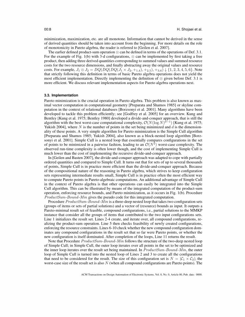
3.3. ImplementationPareto minimization is the crucial operation in Pareto algebra. This problem is also known as max-imal vector computation in computational geometry [Preparata and Shamos 1985] or skyline com-putation in the context of relational databases [Borzsonyi et al. 2001]. Many algorithms have beendeveloped to tackle this problem efficiently; see [Godfrey et al. 2005] for an overview. Kung andBentley [Kung et al. 1975; Bentley 1980] developed a divide-and-conquer approach, that is still thealgorithm with the best worst-case computational complexity, O(N(logN)d−1) [Kung et al. 1975;Yukish 2004], where N is the number of points in the set being minimized and d is the dimension-ality of these points. A very simple algorithm for Pareto minimization is the Simple Cull algorithm[Preparata and Shamos 1985; Yukish 2004], also known as a block-nested loop algorithm [Borz-sonyi et al. 2001]. Simple Cull is a nested loop that essentially compares configurations in the setof points to be minimized in a pairwise fashion, leading to an O(N2) worst-case complexity. Theobserved run-time complexity is often lower though, and the cost of implementing Simple Cull ismuch lower than the cost of implementing the recursive divide-and-conquer approach.
In [Geilen and Basten 2007], the divide-and-conquer approach was adapted to cope with partiallyordered quantities and compared to Simple Cull. It turns out that for sets of up to several thousandsof points, Simple Cull is in practice more efficient than the divide-and-conquer approach. Becauseof the compositional nature of the reasoning in Pareto algebra, which strives to keep configurationsets representing intermediate results small, Simple Cull is in practice often the most efficient wayto compute Pareto points in Pareto-algebraic computations. An additional advantage of Simple Cullin the context of Pareto algebra is that other operations can easily be integrated into the SimpleCull algorithm. This can be illustrated by means of the integrated computation of the product-sumoperation, enforcing resource bounds, and Pareto minimization, as it occurs in Fig. 1(b). ProcedureProductSum-Bound -Min gives the pseudo code for this integrated computation.
Procedure ProductSum-Bound -Min is a three-deep nested loop that takes two configuration sets(groups of items or sets of partial solutions) and a vector of (resource) bounds as input. It outputs aPareto-minimal result set of feasible, compound configurations, i.e., partial solutions to the MMKPinstance that consider all the groups of items that contributed to the two input configurations sets.Line 1 initializes the result set. Lines 2-4 create, and iterate over, all compound configurations, re-alizing the product-sum operation. Line 5 then checks feasibility of newly created configurations,enforcing the resource constraints. Lines 6-10 check whether the new compound configuration dom-inates any compound configurations in the result set that so far were Pareto points, or whether thenew configuration is itself dominated. After completion of the loops, Line 11 returns the result.
Note that Procedure ProductSum-Bound -Min follows the structure of the two-deep nested loopof Simple Cull; in Simple Cull, the outer loop iterates over all points in the set to be optimized andthe inner loop iterates over the result set being maintained. In ProductSum-Bound -Min , the outerloop of Simple Cull is turned into the nested loop of Lines 2 and 3 to create all the configurationsthat need to be considered for the result. The size of this configuration set is N = |C1 × C2|; theworst-case size of the result set is also N (when all compound configurations are Pareto points). The
ACM Transactions on Design Automation of Electronic Systems, Vol. 0, No. 0, Article 00, Pub. date: 0000.
A Fast and Scalable Multi-dimensional Multiple-choice Knapsack Heuristic 00:9
Procedure 1 ProductSum-Bound -Min: Combine two configuration setsInput: C1, C2 configuration sets, b a vector of boundsOutput: result a minimized, compound configuration set, with only feasible configurations
// Initialize the result to the empty set1: result = ∅;
// Iterate over all combinations of configurations2: for all ci ∈ C1 do3: for all cj ∈ C2 do
// Create a compound configuration4: c = ci + cj ;
// Continue only if the compound configuration is feasible5: if feasible(c, b) then
// Minimize the result set// Maintain an attribute to check whether current configuration c is dominated
6: dominated = false;// Iterate over all configurations so far in the result set
7: for all c′ ∈ result do// Check whether the configuration c′ of the result set is dominated; if so, remove it
8: if c ≺ c′ then result = result \ {c′};// Check whether configuration c is itself dominated; if so, stop further minimization
9: else if c′ ≺ c then dominated = true; break;// Add configuration c to the result set if not dominated
10: if not dominated then result = result ∪ {c};11: return result ;
worst-case complexity of ProductSum-Bound -Min is therefore O(N2), i.e., quadratic in terms ofthe size of the set to be minimized, which is exactly the complexity of Simple Cull.
Procedure ProductSum-Bound -Min is the core of our CPH heuristic as presented next. Thelow-overhead, Simple Cull based, integrated implementation of the various operations on the con-figuration sets representing groups of items and partial solutions is more efficient than an explicitimplementation of each of the operations; it is therefore chosen in the implementation of CPH.
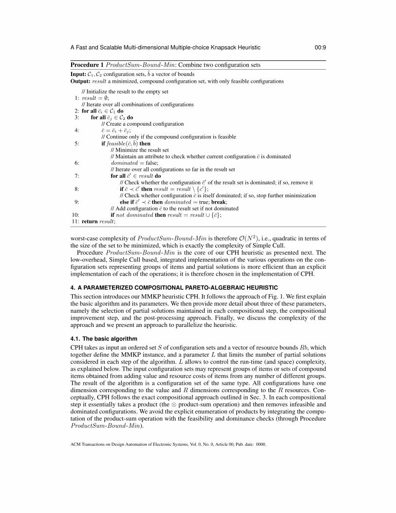
4. A PARAMETERIZED COMPOSITIONAL PARETO-ALGEBRAIC HEURISTICThis section introduces our MMKP heuristic CPH. It follows the approach of Fig. 1. We first explainthe basic algorithm and its parameters. We then provide more detail about three of these parameters,namely the selection of partial solutions maintained in each compositional step, the compositionalimprovement step, and the post-processing approach. Finally, we discuss the complexity of theapproach and we present an approach to parallelize the heuristic.
4.1. The basic algorithmCPH takes as input an ordered set S of configuration sets and a vector of resource bounds Rb, whichtogether define the MMKP instance, and a parameter L that limits the number of partial solutionsconsidered in each step of the algorithm. L allows to control the run-time (and space) complexity,as explained below. The input configuration sets may represent groups of items or sets of compounditems obtained from adding value and resource costs of items from any number of different groups.The result of the algorithm is a configuration set of the same type. All configurations have onedimension corresponding to the value and R dimensions corresponding to the R resources. Con-ceptually, CPH follows the exact compositional approach outlined in Sec. 3. In each compositionalstep it essentially takes a product (the ⊗ product-sum operation) and then removes infeasible anddominated configurations. We avoid the explicit enumeration of products by integrating the compu-tation of the product-sum operation with the feasibility and dominance checks (through ProcedureProductSum-Bound -Min).
ACM Transactions on Design Automation of Electronic Systems, Vol. 0, No. 0, Article 00, Pub. date: 0000.

00:10 H. Shojaei et al.
Procedure 2 CPH: A Pareto-algebraic heuristic for MMKPInput: S a vector of configuration sets, Rb resource bounds, L maximum number of partial solutionsOutput: result, a configuration set, of which any max value configuration is a solution to the MMKP instance
Step 1. // Keep only Pareto pointsFor all Ci ∈ S do min(Ci);
Step 2. // Perform any desirable pre-processingPreProcess(S);
Step 3. // Add aggregate resource usage to all configurationsFor all Ci ∈ S do DQ(Ci, aru);
Step 4. // Optionally, compute an upper bound on the valuevb = SolveLP(S,Rb);
Step 5. // Initialize the set of partial solutions Cps
Cps = S[1]; S = S − S[1];Step 6. // The compositional computations
For all Ci ∈ S do// Select (at most) L partial solutionsCps = SelectPS(Cps, L);// Optionally, improve partial solutionsImprove(Cps);// Select (at most) L configurations from Ci
Ci = SelectPS(Ci, L);// Combine partial solutions with configurations from Ci
Cps = ProductSum-Bound -Min(Cps, Ci, vb;Rb);Step 7. // Perform any desirable post-processing
result = PostProcessing(Cps);Step 8. Return result ;
Procedure CPH provides pseudo-code. CPH gets as input an N -sized vector of configuration setsS, an R-sized vector of resource bounds Rb, and the value for parameter L.
As a first step, Step 1 finds Pareto points in each configuration set. Dominated configurationscannot contribute to an optimal solution of the MMKP instance. A for-loop applies the Pareto-algebraic min operation of Def. 3.1(1).
In Step 2, some form of pre-processing may be performed. For groups with different numbers ofitems, for example, it is beneficial to consider groups with fewer items first. The fewer items thetwo configuration sets being combined in a compositional step have, the faster is the compositionand the more accurate is the result after reducing the set of partial solutions being maintained to Lpartial solutions. Therefore, when groups differ in the number of items, the pre-processing sorts thegroups on their cardinality, in ascending order.
Step 3 adds aggregate resource costs to each configuration, via a derived-quantity operation DQof Def. 3.1(4) with aggregate resource cost function aru . Some operations in CPH may be donein a 2-d value-aggregate resource usage space. Different ways of aggregation may be chosen fordifferent purposes. We discuss several alternatives in Sec. 4.2. Adding aggregate resource usagecosts to configurations makes these configurations (R+ 2)-dimensional. In an implementation, the(R+ 1)-d value-resource usage subspace and the 2-d value-aggregate resource usage subspace canthus efficiently be stored in one data structure.
Step 4 is optional. If enabled, it computes an upper bound on the value for the solution to theMMKP instance. The MMKP instance, which is an integer linear program, is relaxed to a linearprogram (LP). This is done by allowing the decision variables xij to take any real value in the [0, 1]interval and by using ‘=’ instead of ‘≤’ in the set of resource constraints in the MMKP formulation(the third set of constraints). A solution to this LP consists of arbitrary fractions of items of eachgroup that maximize the total value while fully exploiting the available resources. This yields anupper bound for the value of any solution to the original MMKP instance. This upper bound canbe used to prune partial solutions in the same way as resource constraints are used (see Sec. 3.1):
ACM Transactions on Design Automation of Electronic Systems, Vol. 0, No. 0, Article 00, Pub. date: 0000.

A Fast and Scalable Multi-dimensional Multiple-choice Knapsack Heuristic 00:11
if a partial solution has a higher value than the computed upper bound, it cannot be completed to afeasible solution candidate for the MMKP instance. When targeting an embedded implementation ofCPH, computing the value upper bound should preferably be done off-line beforehand (if all relevantinformation is available) or on-line by means of an efficient algorithm to solve LPs. Alternatively,the value bound can simply be omitted because CPH works fine without it. For off-line computationof the value bound, one can use a tool like IBM ILOG Cplex [Cplex 2012]. We experimented withCplex version 9. The computation is very fast and the execution time is negligible for standardMMKP benchmarks. In an actual implementation, for efficiency, the value upper bound may beappended to the resource bounds as a derived quantity.
Step 5 does the initialization for the compositional computations. During the compositional steps,a configuration set Cps of partial solutions is maintained. This set is initialized with the first config-uration set in vector S, S[1], which is subsequently removed from the vector of configurations.
The for-loop in Step 6 implements the compositional steps. It iterates over the list of remainingconfiguration sets. In each iteration, it performs four actions. First, Procedure SelectPS selects (atmost) L partial solutions from configuration set Cps. The details of SelectPS are given in Sec. 4.2.Second, an optional improvement step is performed (Procedure Improve, see Sec. 4.3). Third, (atmost) L configurations from configuration set Ci are selected. Fourth, the selected partial solutionsand new configurations from Ci are combined, through procedure ProductSum-Bound -Min thathas already been discussed in Sec. 3.3.
Procedure ProductSum-Bound -Min is called with Cps and Ci as input configuration sets,and, assuming a value bound is available, with the concatenation vb;Rb of the value bound andthe resource bounds. ProductSum-Bound -Min essentially computes min((Cps ⊗ Ci) ∩ D) withD = {(v, r1, . . . , rR, r) ∈ C | v ≤ vb ∧ ∀1≤k≤R rk ≤ Rb[k]}. The ⊗ product-sum operationcreates all compound configurations. Note that configurations are (R + 2)-d and include aggregateresource cost r. The product-sum operation sums aggregate resource costs of constituent config-urations to compute aggregate resource costs for compound configurations. The set intersectiondefines a constraint operation (Def. 3.1(3)) that allows only configurations that respect both thevalue bound and all the resource capacity constraints. Dominance (the ≺-operation in Lines 8 and9 of ProductSum-Bound -Min and the min operation in the above expression) is not computed inthe (R+2)-d space, but either in the original (R+1)-d space or in the 2-d value-aggregate resourceusage space. The latter is faster and may be employed in on-line embedded applications; the formeris more accurate and may be used when targeting solution quality.
When CPH completes Step 6, Cps contains feasible Pareto-optimal configurations that are allsolution candidates for the considered MMKP instance. Any maximal-value configuration amongthese candidates is typically already a good solution for the MMKP instance. Step 7 of CPH nev-ertheless applies a post-processing algorithm that tries to improve the result of Step 6. The specificpost-processing is again a parameter of CPH. It may be tuned to the situation at hand. Sec. 4.4describes three different post-processing methods that we applied in our CPH implementations.
Finally, Step 8 returns the result, which is a set of configurations, of which any maximal-valueconfiguration is a solution to the MMKP instance.
4.2. Selecting partial solution candidatesWhenever the number of configurations in the compositional steps of CPH, either in the set of partialsolutions or in the additional group of items that is being considered, exceeds threshold L, we needto select L configurations that provide a good approximation of the configuration set at hand. Thisselection needs to be done efficiently, because it is a part of the compositional phase of CPH. Theselection mechanism can be considered to be a parameter of CPH. Any mechanism can be used. Inour implementations so far, we applied a mechanism that determines a selection of partial solutionsin the 2-d value-aggregate resource usage space. Threshold L and the aggregate resource usagefunction aru are parameters of this selection mechanism.
Many MMKP heuristics use the 2-d value-aggregate resource usage space to simplify the searchfor solution candidates. Ref. [Akbar et al. 2006] suggests the transformation of the R resource
ACM Transactions on Design Automation of Electronic Systems, Vol. 0, No. 0, Article 00, Pub. date: 0000.
00:12 H. Shojaei et al.
All configurations (41) Pareto points (20) Selected points (10)
1 /
va
lue
· 1
· 3
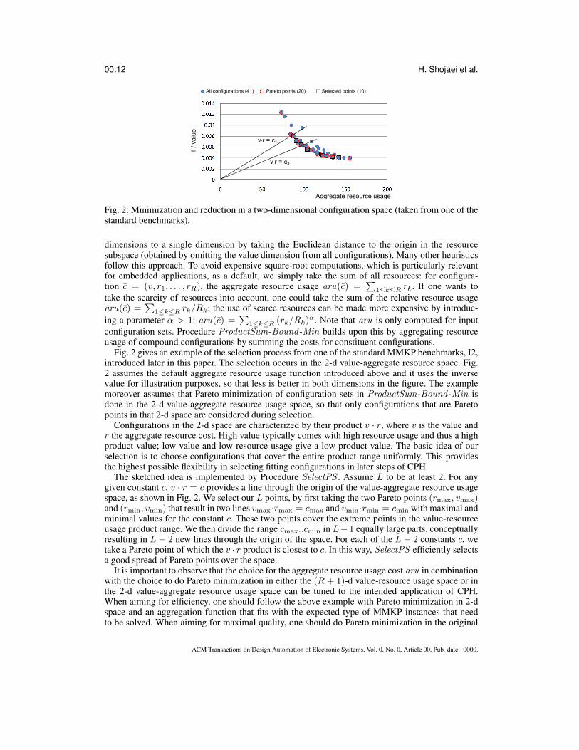
Fig. 2: Minimization and reduction in a two-dimensional configuration space (taken from one of thestandard benchmarks).
dimensions to a single dimension by taking the Euclidean distance to the origin in the resourcesubspace (obtained by omitting the value dimension from all configurations). Many other heuristicsfollow this approach. To avoid expensive square-root computations, which is particularly relevantfor embedded applications, as a default, we simply take the sum of all resources: for configura-tion c = (v, r1, . . . , rR), the aggregate resource usage aru(c) =
∑1≤k≤R rk. If one wants to
take the scarcity of resources into account, one could take the sum of the relative resource usagearu(c) =
∑1≤k≤R rk/Rk; the use of scarce resources can be made more expensive by introduc-
ing a parameter α > 1: aru(c) =∑
1≤k≤R (rk/Rk)α. Note that aru is only computed for input
configuration sets. Procedure ProductSum-Bound -Min builds upon this by aggregating resourceusage of compound configurations by summing the costs for constituent configurations.
Fig. 2 gives an example of the selection process from one of the standard MMKP benchmarks, I2,introduced later in this paper. The selection occurs in the 2-d value-aggregate resource space. Fig.2 assumes the default aggregate resource usage function introduced above and it uses the inversevalue for illustration purposes, so that less is better in both dimensions in the figure. The examplemoreover assumes that Pareto minimization of configuration sets in ProductSum-Bound -Min isdone in the 2-d value-aggregate resource usage space, so that only configurations that are Paretopoints in that 2-d space are considered during selection.
Configurations in the 2-d space are characterized by their product v · r, where v is the value andr the aggregate resource cost. High value typically comes with high resource usage and thus a highproduct value; low value and low resource usage give a low product value. The basic idea of ourselection is to choose configurations that cover the entire product range uniformly. This providesthe highest possible flexibility in selecting fitting configurations in later steps of CPH.
The sketched idea is implemented by Procedure SelectPS . Assume L to be at least 2. For anygiven constant c, v · r = c provides a line through the origin of the value-aggregate resource usagespace, as shown in Fig. 2. We select our L points, by first taking the two Pareto points (rmax, vmax)and (rmin, vmin) that result in two lines vmax ·rmax = cmax and vmin ·rmin = cmin with maximal andminimal values for the constant c. These two points cover the extreme points in the value-resourceusage product range. We then divide the range cmax..cmin in L− 1 equally large parts, conceptuallyresulting in L − 2 new lines through the origin of the space. For each of the L − 2 constants c, wetake a Pareto point of which the v · r product is closest to c. In this way, SelectPS efficiently selectsa good spread of Pareto points over the space.
It is important to observe that the choice for the aggregate resource usage cost aru in combinationwith the choice to do Pareto minimization in either the (R + 1)-d value-resource usage space or inthe 2-d value-aggregate resource usage space can be tuned to the intended application of CPH.When aiming for efficiency, one should follow the above example with Pareto minimization in 2-dspace and an aggregation function that fits with the expected type of MMKP instances that needto be solved. When aiming for maximal quality, one should do Pareto minimization in the original
ACM Transactions on Design Automation of Electronic Systems, Vol. 0, No. 0, Article 00, Pub. date: 0000.

A Fast and Scalable Multi-dimensional Multiple-choice Knapsack Heuristic 00:13
(R+1)-d value-resource usage space. By doing Pareto minimization in the (R+1)-d value-resourceusage space, partial solutions that are Pareto optimal because of low resource usage in any individualdimension are kept; an appropriate aggregate resource usage function then maximizes the chancethat configurations with low resource usage in any dimension corresponding to a scarce resourceis selected in Procedure SelectPS , because it pushes configurations with a high resource usagefor scarce resources to the extreme of the value-resource usage product range, i.e., the v · r rangeintroduced above.
4.3. Compositional improvementDuring the compositional computations, CPH optionally applies an improvement step (ProcedureImprove, Step 6). All the partial solutions in the set Cps provide a good trade off between value andresource costs. Because CPH is a heuristic, the partial solutions may have room for improvementthough, in the sense that a higher value may be obtained with the same or a lower resource usage.The specific improvement step is a parameter that can be tuned to the intended use of CPH. Inour experiments, we applied compositional improvement only when tuning for solution quality. Weimplemented an improvement step that, after a given number of compositional steps, optimizes Cpsusing the IBM ILOG Cplex solver (version 9) [Cplex 2012]. In this implementation of ProcedureImprove, each configuration in Cps is optimized independently. For each configuration, an MMKPinstance is solved to optimality using Cplex. These MMKP instances are much smaller than theoriginal MMKP instance and have tighter resource bounds; they can therefore be solved exactlywithout problems. Assume the last improvement step was executed K compositional steps beforethe current step that performs Improve. Improve then solves for each of the L configurations theMMKP instance that takes (i) the resource usage of the considered configuration in the current setCps as resource bounds; (ii) the result of the last execution of Improve and the K configuration setsCi considered since then as groups. The outcome of Improve is a set of L improved partial solutionsto the original MMKP instance, that is fed into the next compositional step of CPH.
4.4. Post-processingAfter completion of the compositional phase, CPH optionally applies a post-processing step to fur-ther improve the results (Procedure PostProcessing , Step 7 in CPH). The specific post-processingapproach is again a parameter of CPH. We implemented three different methods. ProcedureGrdyPP is a greedy approach that aims for speed and is suitable for on-line use in embeddedapplications; OptPP aims for solution quality, and is intended for off-line use; ImprPP aims fora value improvement within the given resource usage. ImprPP is in fact the same as the composi-tional improvement step of the previous subsection. It provides a compromise between speed andsolution quality and is intended for off-line use.
Recall that all configurations in the set Cps resulting from the compositional phase of CPH arefeasible solution candidates for the MMKP instance. All these solution candidates provide a goodtrade off between value and resource costs, but they may have room for improvement. The highest-value solution candidate can potentially be improved because CPH is a heuristic. The other solutionsmay have room for improvement because, by definition of Pareto-optimality, their resource usage islower than the resource usage of the highest-value solution candidate. It may be that such a solutioncandidate can be further improved than the best solution candidate so far.
The greedy post-processing procedure GrdyPP tries to improve all the solution candidates inset Cps. It first sorts all configurations of the original MMKP instance that contribute to one of thesolution candidates in Cps based on value over aggregate resource-usage ratio (using the default ag-gregate resource usage). The reason to limit attention to configurations that contribute to one of thesolutions in Cps is that, by the fact that they appear in the found Pareto-optimal solution candidatesfor the MMKP instance, those configurations provide a good value-cost ratio. The algorithm theniterates once over this sorted list. For each configuration c in the list, it considers the configurationselected so far for the group to which c belongs in each of the solution candidates in set Cps. If con-figuration c can further improve the solution value without violating the resource constraints, the
ACM Transactions on Design Automation of Electronic Systems, Vol. 0, No. 0, Article 00, Pub. date: 0000.

00:14 H. Shojaei et al.
configuration selected for the group is updated to c. This algorithm is very fast and it turns out fromour experiments that it significantly improves the value when applying CPH in a real-time setting.
The OptPP post-processing procedure uses IBM ILOG Cplex again. It is a brute-force approachthat uses the highest-value solution candidate obtained through the compositional computations asan initial solution for Cplex applied to the original MMKP instance. Cplex is then run up to a giventime limit (or up to completion if it completes within the time limit). As mentioned, an MMKPinstance is an ILP. The Cplex documentation mentions that a good starting point for ILP solving,i.e., in our case a good initial value for the decision variables xi,j in the MMKP instance, has a biginfluence on the speed of the Cplex analysis or the quality of the result if Cplex analysis is terminatedearly. Setting a starting point for ILP solving can be achieved via function CPXcopymipstartand by setting parameter CPX PARAM MIPSTART to 1. Our experiments reported in Sec. 5 showthat the compositional phase of CPH provides a good starting point for further optimization throughCplex, in particular when targeting solution quality and when speed of the analysis is less important.
4.5. Run-time complexityIt is interesting to consider the complexity of CPH. It turns out that, in practice, the running timeof CPH is typically dominated by either the compositional part (when targeting embedded applica-tion and speed of the analysis) or the compositional improvement and post-processing steps (whentargeting off-line usage and quality). We limit our analysis to the compositional part of CPH, Step6. We exclude the compositional improvement and post-processing steps from the analysis, becausetheir complexity depends on the chosen algorithms. We also exclude the first part up to and includ-ing Step 5 of the algorithm. In practice, this part does not really contribute in any substantial way tothe run-time.
Recall that we have N configuration sets in input vector S and assume that Nmax is the maximumnumber of configurations in any of the sets in S. The complexity in each step of the compositionalpart depends on the number of configurations in the considered configuration sets (Cps and Ci) andon parameter L. In each step of the optimization, CPH first limits the size of configuration sets Cpsand Ci to L; the second part invokes ProductSum-Bound -Min on the reduced Cps and Ci. Observethat the size of any of the intermediate Cps results is bounded by L2, because in the worst case allL2 configurations in the product computed in ProductSum-Bound -Min might be Pareto-optimal.The two executions of SelectPS in each iteration of the loop in Step 6 of CPH each require a sortingof the configuration set and a walk through the result to pick L configurations. Therefore, given thatthe size of Cps may be L2 and that the size of Ci is at most Nmax, the complexity of these tworeductions is O(L2 logL) and O(Nmax logNmax). Since the product computed by the two loopsin Lines 2 and 3 of ProductSum-Bound -Min is O(L2), the complexity of ProductSum-Bound -Min is O(L4), as explained in Sec. 3.3. Since CPH does N − 1 compositional steps, the overallcomplexity of the compositional part is O(N (max(Nmax logNmax, L
4))).The compositional part of CPH hardly ever shows its worst-case behavior though, because the
Pareto-dominance checks and the checks on the resource and value bounds prune the search space.Thus, the size of Cps is often much closer to L than to L2. Also, Nmax may be smaller than L, whichalso reduces the practical complexity of every compositional step.
Practical run-time complexity is most important for run-time application of CPH in embeddedreal-time applications. In such applications, we omit the optional compositional improvement step(Procedure Improve in Step 6) and we apply the greedy post-processing step GrdyPP . Because thesize of Cps is often smaller than its worst case, also GrdyPP typically performs better than its worstcase. In addition, often only a small subset of the configurations in the input actually contributes tosolutions found in the compositional phase of CPH, which contributes further to the good practicalperformance of GrdyPP . Given an MMKP instance with N groups, it turns out that the computationtime T (N,L) of CPH with parameter L, with GrdyPP post-processing, and without compositionalimprovement is bounded in practice as follows:
T (N,L) ≤ C · (N · L2 + L), (1)
ACM Transactions on Design Automation of Electronic Systems, Vol. 0, No. 0, Article 00, Pub. date: 0000.
A Fast and Scalable Multi-dimensional Multiple-choice Knapsack Heuristic 00:15
(a) Sequential approach – 1 computer, 7 steps
(b) Parallel approach – 4 computers, 3 rounds of computation
compound
set 2
compound
set 7
compound
set 1
group 2
CPHgroup 1
group 3 group 4
compound
set 11
compound
set 12
compound
set 13
compound
set 14
compound
set 21
compound
set 22
compound
set 31
group 3
CPH
group 8
CPH
CPH
CPHCPH
CPHCPH CPH CPH
group 1 group 2 group 5 group 6 group 7 group 8
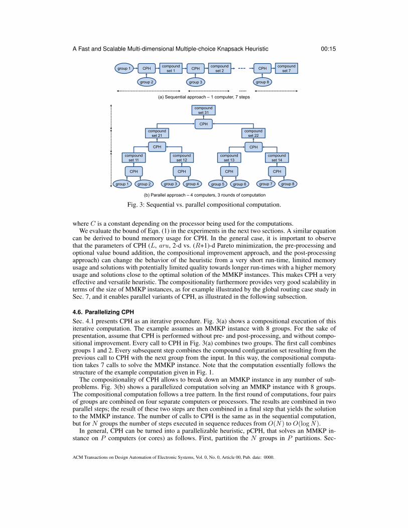
Fig. 3: Sequential vs. parallel compositional computation.
where C is a constant depending on the processor being used for the computations.We evaluate the bound of Eqn. (1) in the experiments in the next two sections. A similar equation
can be derived to bound memory usage for CPH. In the general case, it is important to observethat the parameters of CPH (L, aru , 2-d vs. (R+1)-d Pareto minimization, the pre-processing andoptional value bound addition, the compositional improvement approach, and the post-processingapproach) can change the behavior of the heuristic from a very short run-time, limited memoryusage and solutions with potentially limited quality towards longer run-times with a higher memoryusage and solutions close to the optimal solution of the MMKP instances. This makes CPH a veryeffective and versatile heuristic. The compositionality furthermore provides very good scalability interms of the size of MMKP instances, as for example illustrated by the global routing case study inSec. 7, and it enables parallel variants of CPH, as illustrated in the following subsection.
4.6. Parallelizing CPHSec. 4.1 presents CPH as an iterative procedure. Fig. 3(a) shows a compositional execution of thisiterative computation. The example assumes an MMKP instance with 8 groups. For the sake ofpresentation, assume that CPH is performed without pre- and post-processing, and without compo-sitional improvement. Every call to CPH in Fig. 3(a) combines two groups. The first call combinesgroups 1 and 2. Every subsequent step combines the compound configuration set resulting from theprevious call to CPH with the next group from the input. In this way, the compositional computa-tion takes 7 calls to solve the MMKP instance. Note that the computation essentially follows thestructure of the example computation given in Fig. 1.
The compositionality of CPH allows to break down an MMKP instance in any number of sub-problems. Fig. 3(b) shows a parallelized computation solving an MMKP instance with 8 groups.The compositional computation follows a tree pattern. In the first round of computations, four pairsof groups are combined on four separate computers or processors. The results are combined in twoparallel steps; the result of these two steps are then combined in a final step that yields the solutionto the MMKP instance. The number of calls to CPH is the same as in the sequential computation,but for N groups the number of steps executed in sequence reduces from O(N ) to O(logN ).
In general, CPH can be turned into a parallelizable heuristic, pCPH, that solves an MMKP in-stance on P computers (or cores) as follows. First, partition the N groups in P partitions. Sec-
ACM Transactions on Design Automation of Electronic Systems, Vol. 0, No. 0, Article 00, Pub. date: 0000.

00:16 H. Shojaei et al.
- N=20- P=10- L=100- (R+1)-d min- no pre-processing
N/P N/P
2
N/P N/P
2
N/P N/P
2
N/P N/P
2
N/P N/P
2
2 2
2
2
- Improve- ImprPP
- ImprPP
- ImprPP
- ImprPP
- OptPP
Parameter settings for all CPH calls:
Enabled optimizations:
x Number of configuration sets combined through a CPH call
Total time budget:1200s
Fig. 4: pCPH with 10 processors.
ond, run CPH(p,Rb, L) on each partition p; this can be done in parallel. Third, collect all theresulting compound configuration sets and divide them in as many pairs as possible. Fourth, runCPH(q,Rb, L) on each pair q. Taking pairs maximizes the potential parallelism. If the number ofconfiguration sets is odd, one set is moved to the next round of computations. Fifth, continue thethird and fourth step until only one configuration set remains. This last set gives the solution tothe original MMKP instance. Fig. 4 gives an example parallel computation for 10 processors, i.e.,P = 10, assuming the number of groups N is at least 20.
It is important to observe that parameter settings in pCPH can be chosen separately for each callto CPH. Fig. 4 lists the parameter settings we chose in our experiments reported in the next section.We target pCPH to design-time optimization problems with large MMKP instances. In those cases,parallelism can be optimally exploited. The parameter settings are tuned towards design-time opti-mization. The first round of computations in pCPH solves the largest MMKP instances. Therefore,for this round, compositional improvement (Procedure Improve) is enabled during Step 6 of CPH;ImprPP is performed as post-processing, because it provides a good compromise between speedand quality. During the other rounds of computation no compositional improvement is done, becauseonly two configuration sets are combined each time. ImprPP is still performed as post-processingthough, except during the final step, when OptPP is performed to optimize quality. Since the indi-vidual MMKP instances that are being solved in the parallelized computations are relatively small,a large value of parameter L (that sets the number of maintained partial solutions) is possible. Weused L = 100 in our experiments. The default setting to do no pre-processing is selected. Paretopoints in ProductSum-Bound -Min are computed in the original (R + 1)-d value-resource-usagespace, prioritizing quality over speed. Assuming that the total available time budget is sufficient tocomplete the parallelized computations up to the last step, a time budget for the overall computationcan be set by setting an appropriate time budget for OptPP . In the experiments reported in the nextsection, we set the overall time budget to 1200s.
Note that pCPH is not a parallelization of CPH in the classical sense. Due to the non-uniformparameter settings for the various sub-computations performed in the various parallel rounds, pCPHperforms an algorithm that differs from the algorithm implemented by CPH. Since both pCPH andCPH allow to set the overall time budget to be spent for the analysis, we envision the use of pCPHwith the same total time budget as the budget that would be available to CPH. pCPH can then exploitany processors that are available, according to the scheme laid out in Fig. 4. The aim is to improvesolution quality and not to speed up the computation. As the results reported in the next sectionshow, pCPH gives better results than CPH in the same time budget.
ACM Transactions on Design Automation of Electronic Systems, Vol. 0, No. 0, Article 00, Pub. date: 0000.

A Fast and Scalable Multi-dimensional Multiple-choice Knapsack Heuristic 00:17
Table I: MMKP benchmarks of [MMKP benchmarks 2010], with the number of groups (N ), the number ofitems per group i (Ni), the number of resource dimensions (R), and the optimal value (val.) or an upper boundon this value (entries marked with *).
Bench. N Ni R val. Bench. N Ni R val.
I1 5 5 5 173 INST4 70 10 10 14478*I2 10 5 5 364 INST5 75 10 10 17078*I3 15 10 10 1602 INST6 75 10 10 16856*I4 20 10 10 3597 INST7 80 10 10 16459*I5 25 10 10 3905.7 INST8 80 10 10 17533*I6 30 10 10 4799.3 INST9 80 10 10 17779*I7 100 10 10 24607* INST10 90 10 10 19337*I8 150 10 10 36904* INST11 90 10 10 19462*I9 200 10 10 49193* INST12 100 10 10 21757*I10 250 10 10 61486* INST13 100 30 10 21593*I11 300 10 10 73797* INST14 150 30 10 32887*I12 350 10 10 86100* INST15 180 30 10 39174*I13 400 10 10 98448* INST16 200 30 10 43379*
INST17 250 30 10 54372*INST1 50 10 10 10753* INST18 280 20 10 60478*INST2 50 10 10 13633* INST19 300 20 10 64943*INST3 60 10 10 10985* INST20 350 20 10 75627*
Note that cost of communication is small compared to the cost of computation. Only the Paretopoints obtained for each of the sub-problems need to be communicated. Computation thereforedominates the total analysis time. In the current version of pCPH the number of processors thatcan be used in each round of computation, halves. As future work, it would be interesting to devisedifferent parallelization schemes of the computations and/or load balancing schemes that optimallyexploit the available number of processors.
5. EVALUATION OF CPH ON MMKP BENCHMARKSThe previous section has introduced our heuristic CPH, the various parameters that allow tuningof the procedure, and a parallel variant of CPH. In this section, we experimentally investigate thevarious aspects of CPH on standard benchmarks. First, Sec. 5.1 explains the experimental setup.Second, Sec. 5.2 illustrates how to trade off analysis time with solution quality. Third, in Sec. 5.3,we evaluate CPH for real-time analysis. Finally, in Sec, 5.4, CPH scalability in terms of solutionquality is evaluated. The latter includes an evaluation of pCPH, the parallelizable variant of CPH.
5.1. Experimental setupThe experiments performed in this section use standard MMKP benchmarks [MMKP benchmarks2010] that are used in most of the work on MMKP. Table I summarizes the characteristics of thebenchmarks. In line with [Ykman-Couvreur et al. 2006], we divide the benchmark problems intotwo groups. Instances I1-I6 are considered representatives for real-time embedded applications.Heuristics targeting this class of applications should emphasize efficiency of the analysis. The sec-ond group of benchmarks, I7-I13 and INST01-INST20, provides larger test cases for quality-drivenapproaches to solving MMKP. As Table I shows, the optimal values for I1-I6 are known; for theother benchmarks, only an upper bound on the optimal value is known, obtained by solving theMMKP instances as a linear program.
In the standard benchmarks, all groups of a benchmark have an equal number of items; further, thenumber of resource dimensions is fixed and all items use resources in all resource dimensions with auniform distribution. To cover a wider range of MMKP instances in our evaluations, we constructedadditional benchmarks, described in Table II, that exhibit a more irregular structure. The numberof items per group in a benchmark varies and an item does not necessarily use resources in allthe resource dimensions. Also the new benchmarks are divided into small benchmarks for real-time analysis, RTI7-RT13, and large benchmarks, INST21-INST30, for evaluation of scalabilityand solution quality. The new benchmarks are available via [MMKP benchmarks 2012]. For RTI7-
ACM Transactions on Design Automation of Electronic Systems, Vol. 0, No. 0, Article 00, Pub. date: 0000.

00:18 H. Shojaei et al.
Table II: Irregular MMKP benchmarks [MMKP benchmarks 2012], with the number of groups (N ), themaximum number of items per group i (max Ni), the number of resource dimensions (R), and the optimalvalue (val.) or an upper bound on this value (entries marked with *).
Bench. N max Ni R val. Bench. N max Ni R val.
RTI7 10 10 10 564 INST21 100 10 10 44315*RTI8 20 10 10 6576 INST22 100 10 20 42076*RTI9 30 10 10 7806 INST23 100 10 30 42763*RTI10 30 20 10 7031 INST24 100 10 40 42252*RTI11 30 20 20 6880 INST25 100 20 10 44201*RTI12 40 10 10 11564 INST26 100 20 20 45011*RTI13 50 10 10 10561 INST27 200 10 10 87650*
INST28 300 10 10 134672*INST29 400 10 10 179245*INST30 500 10 10 214257*
58800
58900
59000
59100
59200
59300
1.60ms
(5)
5.80ms
(7)
8.30ms
(10)
14.00ms
(15)
27.80ms
(20)
Va
lue
Time
(Parameter L)
0
10
20
30
40
50
60
12
(59101)
16
(59128)
21
(59190)
24
(59207)
27
(59224)
Tim
e(m
s)
Parameter L
(Value)
TB:10ms
TB:20ms
TB:30ms
TB:40ms
TB:50ms
(b)(a)
Fig. 5: Trading off value vs. computation time (a) and controlling time budgets (b), illustrated forbenchmark I10.
RT13, Table II gives the optimal values; for the other benchmarks an upper bound on the value wascomputed by relaxing the MMKP instance to a linear program.
We implemented CPH in the C programming language. Where Cplex [Cplex 2012] is used, thisrefers to the academic edition, version 9, with the default parameter settings. All experiments in thissection were done on a PC with a 2.8Ghz Intel CPU and 12 GB of memory.
5.2. Trading off time and qualityIn the first experiment, we show that CPH allows computation time and solution quality to be tradedoff, and that the computation time can be bounded beforehand. These aspects are particularly rel-evant when MMKP instances need to be solved under time constraints. We take CPH withoutpre-processing but with value bound, without intermediate compositional optimization steps andwith greedy post-processing (Procedure GrdyPP ). Pareto minimization is done in the projected 2-dvalue-aggregate resource usage space with the default aggregation function.
Fig. 5(a) illustrates the trade-off between quality of the solution and the computation time forCPH. Results are reported for benchmark I10, for different values of L, i.e., the number of interme-diate partial solutions kept in the compositional computations. These results are illustrative for allbenchmarks, and confirm that the trade-off can be controlled by L.
An interesting use of this trade off, is that it allows to limit the computation time to small, pre-defined time bounds, via Eqn. (1). We used 10, 20, 30, 40, and 50 ms as bounds. To compute L,we use Eqn. (1) with constant C = 0.0004. This value was measured on the used PC configurationusing one of the benchmarks as a test case. Fig. 5(b) again shows the results for MMKP benchmarkI10. The figure shows the time bound and the actual computation time of CPH in milliseconds, the
ACM Transactions on Design Automation of Electronic Systems, Vol. 0, No. 0, Article 00, Pub. date: 0000.

A Fast and Scalable Multi-dimensional Multiple-choice Knapsack Heuristic 00:19
value of the computed parameter L, and the value of the obtained solution. All the results (for allbenchmarks) confirm that the bound of Eqn. (1) is conservative.
5.3. Evaluating CPH for real-time analysisIn our second set of experiments, we evaluate the real-time performance of CPH, using the mecha-nism to control the time budget illustrated in the previous subsection. We compare CPH to the fastestamong the other MMKP heuristics to date, RTM [Ykman-Couvreur et al. 2006; Ykman-Couvreuret al. 2011]. We take CPH without pre-processing and without compositional optimization, withgreedy post-processing, and with Pareto minimization in 2-d space. The default resource usage ag-gregation is used unless explicitly stated otherwise. The value of parameter L is determined by theavailable time budget. We implemented the RTM heuristic in the C programming language, in linewith the implementation of CPH. For these comparative experiments we use the PC setup describedabove, for efficiency and flexibility in doing the experiments. In the next section, we evaluate CPHon an embedded platform.
Table III: Comparison with RTM [Ykman-Couvreur et al. 2006; Ykman-Couvreur et al. 2011] for real-timebenchmarks. Computation times in ms.
Bench. Opt. val. RTM CPH (t≤t(RTM))
val t(ms) L val t(ms) %
I1 173 148 0.04 4 157 0.03 6.08I2 364 327 0.06 4 327 0.04 0.00I3 1602 1407 0.13 4 1410 0.11 0.21I4 3597 3325 0.16 4 3310 0.15 -0.45I5 3905.7 3705 0.19 4 3900 0.16 5.26I6 4799.3 4313 0.24 4 4651 0.20 7.84
avg 3.16
Table III shows the results of our experiments with the standard benchmarks meant for real-timeanalysis, I1-I6. We took the time needed by RTM as the time bound for CPH. The ‘t≤ t(RTM)’part of the table gives the results. The ‘val’ and ‘t(ms)’ columns report obtained values per MMKPinstance and computation times in milliseconds, respectively. The ‘L’ labeled column gives the valueof L computed from Eqn. (1). As expected, execution times for CPH are, with the computed valuefor L, always within the bound given by RTM for the corresponding case. The solution quality ofthe two approaches is compared in the ‘%’ column, which gives the relative performance of CPHcompared to RTM. On average, we may conclude that our obtained solution quality is slightly betterthan that of RTM when given equal time budgets. The actual computation time for CPH is alwaysless than the time needed by RTM. Other advantages of our approach are that the computation-timebound can be set beforehand and that solution quality can be improved by increasing L if the timebudget allows. Both are not possible for RTM.
We also compared RTM and CPH on the new irregular benchmarks, RTI7-RTI13. Table IV showsthe results. An important aspect is that RTM assumes that the combination of items with the lowestvalues in each group always provides a feasible solution. While this is true for all the originalMMKP benchmarks, this is not necessarily true in general, as we for example observed in our globalrouting case study (Sec. 7). Also in the newly generated irregular benchmarks, the combination oflowest-value items leads in some cases to an infeasible solution. Hence, the original RTM approachis not directly applicable to these new benchmarks. To tackle this problem, we added an initialstep to RTM in which a feasible initial solution is found and passed to RTM. If the starting solutionassumed by RTM is infeasible, this initial step first sorts all the items in ascending order of aggregateresource usage; it then visits the items in the list one by one, swapping an item from the list witha selected item if this decreases the usage of at least one resource dimension without hurting anyother dimension. As soon as a feasible solution is found, it is passed to the original RTM heuristic.
ACM Transactions on Design Automation of Electronic Systems, Vol. 0, No. 0, Article 00, Pub. date: 0000.

00:20 H. Shojaei et al.
Table IV: Results for irregular real-time benchmarks. Time in ms.
Bench. Opt. val RTM CPH (t≤t(RTM))default aggregation scarcity-aware aggr.
val t(ms) L val t(ms) % L val t(ms) %
RTI7 564 534 0.01 4 534 0.01 0.00 4 534 0.01 0.00RTI8 6576 +6000 0.06 4 6000 0.06 0.00 4 6130 0.06 2.17RTI9 7806 +5445 0.18 4 6817 0.16 25.20 4 7367 0.17 35.30RTI10 7031 5432 0.27 4 6089 0.26 12.09 4 6096 0.27 12.22RTI11 6880 +5208 0.49 4 5277 0.48 1.32 4 5449 0.45 4.63RTI12 11564 10746 0.12 4 10746 0.11 0.00 4 10860 0.12 1.06RTI13 10561 +8139 0.21 4 8636 0.21 6.11 4 8097 0.20 -0.52
avg 6.26 7.84
Table V: The impact of greedy post-processing (Procedure GrdyPP ). Computation times in ms.
CPH (t≤t(RTM))w/o pp with GrdyPP
Bench. L val t(ms) L val t(ms) %
I1 11 154 0.03 4 157 0.03 1.95I2 10 325 0.06 4 327 0.04 0.62I3 9 1337 0.14 4 1410 0.11 5.46I4 9 2870 0.17 4 3310 0.15 15.33I5 9 3900 0.17 4 3900 0.16 0.00I6 9 4554 0.24 4 4651 0.20 2.13
avg 4.25
Benchmarks marked with “+” in the RTM column of Table IV require to compute an initial solutionto enable RTM.
CPH is directly applicable to the new benchmarks. It does not assume any specific informationabout an MMKP instance. Moreover, CPH can take advantage of irregularity in an MMKP instanceto improve the quality and speed of the procedure. The run-time of CPH strongly depends on thenumber of items per group. Run-time improves if groups with less items are considered first. Thisalso decreases the need to eliminate partial solutions in the SelectPP procedure, which improvessolution quality. Therefore, for the irregular benchmarks RTI7-RTI13, we enable the pre-processingstep, Step 1 of CPH. We sort the groups of items in ascending order of cardinality and start CPHwith the group that has the least items. For these irregular benchmarks, we experimented with boththe default aggregate resource usage function aru(c) =
∑1≤k≤R rk for c = (v, r1, . . . , rR) and
with the function aru(c) =∑
1≤k≤R (rk/Rk)2 that penalizes high usage of scarce resources (see
Sec. 4.2). Given the irregularity, the latter may give better results.Table IV compares the two instances of CPH with RTM for RTI7-RTI13. We again considered
the RTM computation time as time bound for CPH. Where relevant, the time to compute an initialsolution for RTM is included in the reported time for RTM. For CPH, the time for pre-processingis included. The results show that with one exception CPH provides better results than RTM. Usingscarcity-aware resource usage aggregation in CPH gives in general slightly better results than thedefault aggregation, showing that it may be beneficial to adapt the aggregation function to the typeof groups that occur in the MMKP instance.
As a final experiment in this subsection, we explore the impact of post-processing in CPH. Wemake a comparison to the CPH variant of [Shojaei et al. 2009] that does not include post-processing.We again considered the computation time needed by the RTM heuristic as a bound for the run-time for CPH. Using Eqn. (1) and a variant of it without the C · L factor for CPH without post-processing, we computed the values of L for both CPH with and without post-processing. TableV gives the results. The ‘%’ column shows the improvement in terms of value obtained by greedy
ACM Transactions on Design Automation of Electronic Systems, Vol. 0, No. 0, Article 00, Pub. date: 0000.

A Fast and Scalable Multi-dimensional Multiple-choice Knapsack Heuristic 00:21
post-processing. CPH with post-processing is always at least as fast as CPH without post-processingwhile at the same time it always gives a value that is at least as good as without post-processing.
The results of Tables IV and V show that the parameterized version of CPH as presented in thecurrent paper outperforms the earlier version presented in [Shojaei et al. 2009].
5.4. Evaluating the scalability of CPH for solution qualityIn the final set of experiments in this section, we compare CPH with the state-of-the-art heuristics forsolution quality [Crevits et al. 2012; Cherfi 2009]. The goal is to evaluate scalability of CPH both interms of solution quality and run-time. We tune CPH to prioritize quality by including Cplex-basedcompositional improvement (Procedure Improve in Step 6 of CPH) and post-processing (Proce-dure OptPP ). Procedure Improve is applied every 10 iterations of the main compositional loop.We set parameter L to 10 to maintain 10 partial solutions during each of the compositional steps;we use the default resource-usage aggregation for selecting partial solutions. We do not performpre-processing, but we do compute a value upper bound in Step 4 of CPH. Since speed is less im-portant than quality, we compute Pareto points in ProductSum-Bound -Min in the original (R+1)-dimensional value-resource usage space.
Table VI: Comparison with quality-based MMKP approaches.
Benchmark Previous Results Cplex CPH + OptPP pCPH
ILPH IMIPH IIRH BLHG t=1200s t=3600s Compos. t=1200s t=1200s[Crevits et al. 2012] [Cherfi 2009] value time
I7 24591 24587 24592 24587 24584 24589 24584 128 24592 24592I8 36888 36889 36888 36894 36885 36886 36843 156 36885 36886I9 49174 49183 49179 49179 49171 49176 49139 188 49179 49185I10 61469 61471 61466 61464 61464 61465 61423 228 61464 61465I11 73784 73779 73779 73783 73777 73788 73739 233 73780 73782I12 86091 86083 86091 86080 86080 86080 86035 252 86081 86084I13 98435 98445 98433 98438 98433 98437 98380 302 98433 98437INST1 10738 10728 10728 10738 10720 10738 10693 101 10727 10733INST2 13598 13598 13598 13598 13598 13598 13580 120 13598 13598INST3 10949 10943 10949 10944 10942 10946 10897 98 10955 10955INST4 14442 14445 14446 14442 14442 14447 14411 130 14452 14452INST5 17058 17055 17057 17053 17058 17059 17025 131 17055 17059INST6 16835 16832 16832 16827 16830 16832 16791 115 16827 16830INST7 16440 16440 16440 16440 16440 16440 16397 121 16440 16440INST8 17510 17511 17510 17510 17507 17513 17474 145 17507 17509INST9 17760 17760 17753 17761 17754 17754 17705 126 17757 17754INST10 19320 19320 19314 19316 19301 19306 19266 127 19314 19316INST11 19446 19446 19446 19441 19429 19435 19396 114 19441 19441INST12 21733 21738 21738 21732 21732 21732 21698 137 21738 21738INST13 21577 21580 21577 21577 21577 21577 21569 209 21577 21577INST14 32873 32872 32872 32874 32871 32871 32850 192 32872 32872INST15 39161 39160 39162 39160 39159 39160 39151 320 39160 39161INST16 43366 43363 43363 43362 43363 43364 43343 238 43363 43363INST17 54361 54360 54358 54360 54360 54360 54344 394 54360 54360INST18 60467 60467 60465 60464 60464 60467 60454 213 60465 60464INST19 64930 64932 64929 64925 64930 64931 64914 244 64931 64932INST20 75613 75611 75613 75612 75613 75615 75595 238 75613 75615
Best values 11/4 11/4 7/1 6/3 6/2 10/5
Table VI presents the results. Columns 2 to 5 report the results of the state-of-the-art heuristics.Since this version of CPH uses Cplex, we also solved the benchmarks using pure Cplex, both witha 1200s and a 1 hour time limit, to be used as a reference. Columns 6-7 give the results. Columns8-9 show the values and computation times of the compositional part in CPH, including the compo-sitional improvement step, but before post-processing. Column 10 shows the final result after Cplexpost-processing, where we consider a time bound of 1200s on the total time available to CPH. Thatis, the time bound for Cplex post-processing is set to the difference between 1200s and the run-time
ACM Transactions on Design Automation of Electronic Systems, Vol. 0, No. 0, Article 00, Pub. date: 0000.
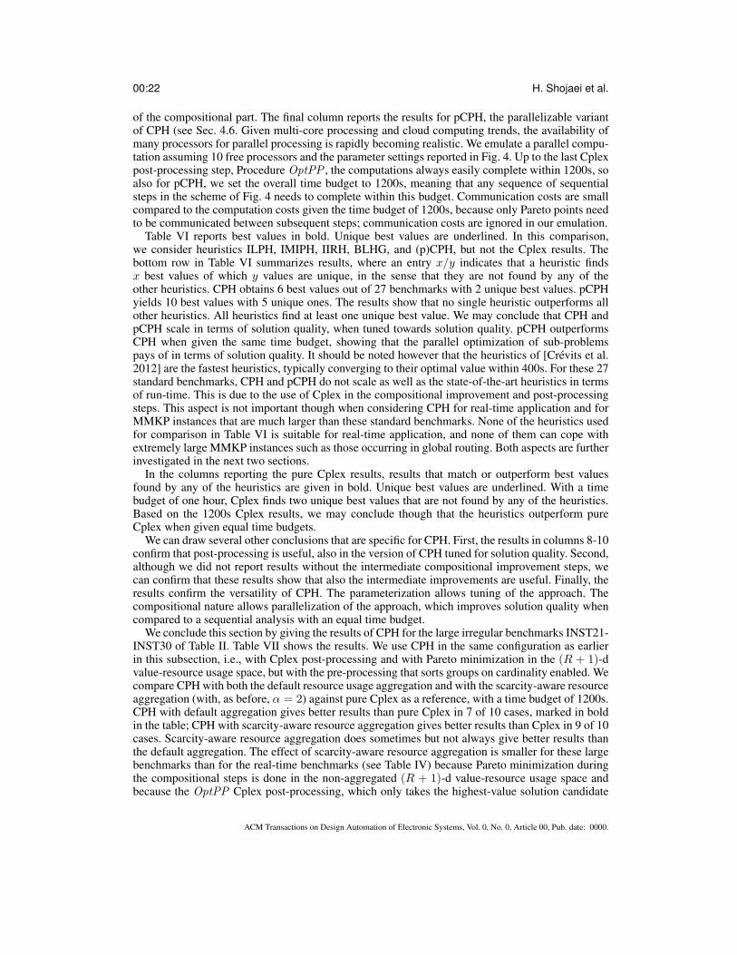
00:22 H. Shojaei et al.
of the compositional part. The final column reports the results for pCPH, the parallelizable variantof CPH (see Sec. 4.6. Given multi-core processing and cloud computing trends, the availability ofmany processors for parallel processing is rapidly becoming realistic. We emulate a parallel compu-tation assuming 10 free processors and the parameter settings reported in Fig. 4. Up to the last Cplexpost-processing step, Procedure OptPP , the computations always easily complete within 1200s, soalso for pCPH, we set the overall time budget to 1200s, meaning that any sequence of sequentialsteps in the scheme of Fig. 4 needs to complete within this budget. Communication costs are smallcompared to the computation costs given the time budget of 1200s, because only Pareto points needto be communicated between subsequent steps; communication costs are ignored in our emulation.
Table VI reports best values in bold. Unique best values are underlined. In this comparison,we consider heuristics ILPH, IMIPH, IIRH, BLHG, and (p)CPH, but not the Cplex results. Thebottom row in Table VI summarizes results, where an entry x/y indicates that a heuristic findsx best values of which y values are unique, in the sense that they are not found by any of theother heuristics. CPH obtains 6 best values out of 27 benchmarks with 2 unique best values. pCPHyields 10 best values with 5 unique ones. The results show that no single heuristic outperforms allother heuristics. All heuristics find at least one unique best value. We may conclude that CPH andpCPH scale in terms of solution quality, when tuned towards solution quality. pCPH outperformsCPH when given the same time budget, showing that the parallel optimization of sub-problemspays of in terms of solution quality. It should be noted however that the heuristics of [Crevits et al.2012] are the fastest heuristics, typically converging to their optimal value within 400s. For these 27standard benchmarks, CPH and pCPH do not scale as well as the state-of-the-art heuristics in termsof run-time. This is due to the use of Cplex in the compositional improvement and post-processingsteps. This aspect is not important though when considering CPH for real-time application and forMMKP instances that are much larger than these standard benchmarks. None of the heuristics usedfor comparison in Table VI is suitable for real-time application, and none of them can cope withextremely large MMKP instances such as those occurring in global routing. Both aspects are furtherinvestigated in the next two sections.
In the columns reporting the pure Cplex results, results that match or outperform best valuesfound by any of the heuristics are given in bold. Unique best values are underlined. With a timebudget of one hour, Cplex finds two unique best values that are not found by any of the heuristics.Based on the 1200s Cplex results, we may conclude though that the heuristics outperform pureCplex when given equal time budgets.
We can draw several other conclusions that are specific for CPH. First, the results in columns 8-10confirm that post-processing is useful, also in the version of CPH tuned for solution quality. Second,although we did not report results without the intermediate compositional improvement steps, wecan confirm that these results show that also the intermediate improvements are useful. Finally, theresults confirm the versatility of CPH. The parameterization allows tuning of the approach. Thecompositional nature allows parallelization of the approach, which improves solution quality whencompared to a sequential analysis with an equal time budget.
We conclude this section by giving the results of CPH for the large irregular benchmarks INST21-INST30 of Table II. Table VII shows the results. We use CPH in the same configuration as earlierin this subsection, i.e., with Cplex post-processing and with Pareto minimization in the (R + 1)-dvalue-resource usage space, but with the pre-processing that sorts groups on cardinality enabled. Wecompare CPH with both the default resource usage aggregation and with the scarcity-aware resourceaggregation (with, as before, α = 2) against pure Cplex as a reference, with a time budget of 1200s.CPH with default aggregation gives better results than pure Cplex in 7 of 10 cases, marked in boldin the table; CPH with scarcity-aware resource aggregation gives better results than Cplex in 9 of 10cases. Scarcity-aware resource aggregation does sometimes but not always give better results thanthe default aggregation. The effect of scarcity-aware resource aggregation is smaller for these largebenchmarks than for the real-time benchmarks (see Table IV) because Pareto minimization duringthe compositional steps is done in the non-aggregated (R + 1)-d value-resource usage space andbecause the OptPP Cplex post-processing, which only takes the highest-value solution candidate
ACM Transactions on Design Automation of Electronic Systems, Vol. 0, No. 0, Article 00, Pub. date: 0000.
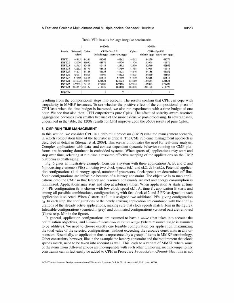
A Fast and Scalable Multi-dimensional Multiple-choice Knapsack Heuristic 00:23
Table VII: Results for large irregular benchmarks.
t=1200s t=3600s
Bench. Relaxed Cplex CPH+OptPP Cplex CPH+OptPPvalue default aggr. scarc.-aw. aggr. default aggr. scarc.-aw. aggr.
INST21 44315 44246 44262 44262 44262 44270 44270INST22 42076 41930 41976 44976 41976 41976 41976INST23 42763 42488 42488 42502 42550 42560 42562INST24 42252 41776 41918 41910 41918 41918 41918INST25 44201 44128 44138 44128 44146 44156 44152INST26 45011 44806 44806 44832 44835 44869 44869INST27 87650 87588 87616 87600 87600 87616 87616INST28 134672 134594 134634 134634 134610 134634 134634INST29 179245 179168 179186 179186 179202 179204 179206INST30 214257 214132 214132 214198 214198 214198 214198
Improv. 7 9 7 7
resulting from the compositional steps into account. The results confirm that CPH can cope withirregularity in MMKP instances. To see whether the positive effect of the compositional phase ofCPH lasts when the time budget is increased, we also ran experiments with a time budget of onehour. We see that also then, CPH outperforms pure Cplex. The effect of scarcity-aware resourceaggregation becomes even smaller because of the more extensive post-processing. In several cases,underlined in the table, the 1200s results for CPH improve upon the 3600s results of pure Cplex.
6. CMP RUN-TIME MANAGEMENTIn this section, we consider CPH in a chip-multiprocessor (CMP) run-time management scenario,in which computation time of the heuristic is critical. The CMP run-time management approach isdescribed in detail in [Shojaei et al. 2009]. This scenario motivates the need for real-time analysis.Complex applications with data- and context-dependent dynamic behavior running on CMP plat-forms are becoming dominant in embedded systems. When (parts of) applications may start andstop over time, selecting at run-time a resource-effective mapping of the applications on the CMPplatforms is challenging.
Fig. 6 gives an illustrative example. Consider a system with three applications A, B, and C and6 processing elements (PEs) allowing two clock speeds (ck1 and ck2, ck1<ck2). Potential applica-tion configurations (4-d: energy, speed, number of processors, clock speed) are determined off-line.Some configurations are infeasible because of a latency constraint. The objective is to map appli-cations onto the CMP so that latency and resource constraints are met and energy consumption isminimized. Applications may start and stop at arbitrary times. When application A starts at time0, 4-PE configuration c1 is chosen with low clock speed ck1. At time t1, application B starts andamong all possible combinations, configuration c2 with fast clock ck2 and 2 PEs assigned to eachapplication is selected. When C starts at t2, it is assigned two additional PEs, giving configurationc3. In each step, the configurations of the newly arriving application are combined with the config-urations of the already active applications, making sure that clock speeds match (Join in the figure).Infeasible configurations (denoted in grey) and dominated configurations (crossed out) are removed(Const resp. Min in the figure).
In general, application configurations are assumed to have a value (that takes into account theoptimization objectives) and a multi-dimensional resource usage (where resource usage is assumedto be additive). We need to choose exactly one feasible configuration per application, maximizingthe total value of the selected configurations, without exceeding the resource constraints in any di-mension. Essentially, an application thus is represented by a group of items in MMKP terminology.Other constraints, however, like in the example the latency constraint and the requirement that clockspeeds match, need to be taken into account as well. This leads to a variant of MMKP where someof the items from different groups are incompatible with each other. Enforcing such incompatibilityconstraints can in fact easily be added to CPH in Procedure ProductSum-Bound -Min; this is not
ACM Transactions on Design Automation of Electronic Systems, Vol. 0, No. 0, Article 00, Pub. date: 0000.
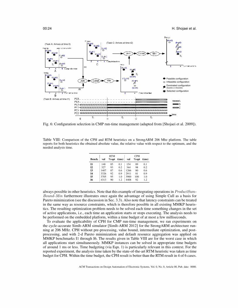
00:24 H. Shojaei et al.
Selected configuration
Dominated configuration(feasible or infeasible)
Infeasible configuration
Feasible configuration
(Task B: Arrives at time t1)
(Task A: Arrives at time 0)(Task C: Arrives at time t2)
c1
c1
c2
c2 c3
c3
Fig. 6: Configuration selection in CMP run-time management (adapted from [Shojaei et al. 2009]).
Table VIII: Comparison of the CPH and RTM heuristics on a StrongARM 206 Mhz platform. The tablereports for both heuristics the obtained absolute value, the relative value with respect to the optimum, and theneeded analysis time.
RTM CPHBench. val %opt t(ms) val %opt t(ms)
I1 148 85 0.1 154 89 0.1I2 327 93 0.2 344 98 0.2I3 1407 87 0.6 1266 80 0.6I4 3326 92 0.9 2911 81 0.9I5 3705 95 1.0 3900 100 1.0I6 4313 90 1.2 4408 92 1.2
always possible in other heuristics. Note that this example of integrating operations in ProductSum-Bound -Min furthermore illustrates once again the advantage of using Simple Cull as a basis forPareto minimization (see the discussion in Sec. 3.3). Also note that latency constraints can be treatedin the same way as resource constraints, which is therefore possible in all existing MMKP heuris-tics. The resulting optimization problem needs to be solved each time something changes in the setof active applications, i.e., each time an application starts or stops executing. The analysis needs tobe performed on the embedded platform, within a time budget of at most a few milliseconds.
To evaluate the applicability of CPH for CMP run-time management, we ran experiments onthe cycle-accurate SimIt-ARM simulator [SimIt-ARM 2012] for the StrongARM architecture run-ning at 206 MHz. CPH without pre-processing, value bound, intermediate optimization, and post-processing, and with 2-d Pareto minimization and default resource aggregation was applied onMMKP benchmarks I1 through I6. The results given in Table VIII are for the worst case in whichall applications start simultaneously. MMKP instances can be solved in appropriate time budgetsof around 1 ms or less. Time budgeting (via Eqn. 1) is particularly relevant in this context. For thereported experiment, the analysis time taken by the state-of-the-art RTM heuristic was taken as timebudget for CPH. Within the time budget, the CPH result is better than the RTM result in 4 of 6 cases.
ACM Transactions on Design Automation of Electronic Systems, Vol. 0, No. 0, Article 00, Pub. date: 0000.

A Fast and Scalable Multi-dimensional Multiple-choice Knapsack Heuristic 00:25
RTM CPH
Fig. 7: An illustration of compositional MMKP solving, using benchmark I5, with (a) 5 applicationsstarting at a time, and (b) 1 application starting at a time (from [Shojaei et al. 2009]).
Another important aspect in this particular application of CPH is compositionality. Fig. 7, takenfrom [Shojaei et al. 2009], compares the performance of CPH with the RTM heuristic, on the Strong-ARM platform, for benchmark I5 with L = 10 and assuming that applications start 5 at a time (a)or 1 at a time (b). The results illustrate that CPH can be applied incrementally and that the perfor-mance does not depend on the number of active applications (i.e., the number of groups alreadycovered in the compositional computation). RTM needs to solve the complete MMKP instance forall applications each time, which results in increasing execution times when more applications areactive. Compositionality only applies when applications start. When applications stop, i.e., when anitem from one group in the MMKP has to be removed from the solution, both RTM and CPH needto recompute the full remaining MMKP instance to optimize the mapping. In practice, this is not aproblem. If an application stops, it is guaranteed that the remaining configuration is still feasible, sothe reconfiguration process is not time critical.
7. GLOBAL ROUTINGGlobal routing is the step in the physical implementation of Integrated Circuits (ICs) that plans thewiring between nano-scale components. Today’s ICs contain millions of nets that should be routed.Each route is a complex 3-d structure, spanning over many metal layers. Global routing thus is avery large-sized combinatorial optimization problem. Scalability of solution heuristics with respectto the size of an MMKP instance is essential. This case study illustrates the application of CPH in adesign-time optimization problem.
In global routing, we are given a grid-graph G. Each net is represented by a subset of vertices thatdenote the locations of its terminals on the grid. To route a net, its terminals should be connectedusing the edges in G. For a given route of a net, its wirelength is the length of the Steiner treeconnecting its terminals. Each edge in G has a capacity representing the maximum number of routesthat can pass the edge without over-utilizing the routing resource associated with the edge. The goalof global routing is to route all the nets subject to the edge capacity constraints, while minimizingthe summed wirelength.
Global routing problem variants can be modeled as MMKP instances [Shojaei et al. 2010]. Toillustrate scalability of CPH, we discuss collaborative global routing in which wirelength is mini-mized by reusing good routes found by different existing routing tools. Each net is represented as agroup of items in which an item is a candidate route for the net. The wirelength corresponding to acandidate route is its value (smaller values being better). Each edge in the grid-graph G correspondsto a resource. The resource usage of a candidate route is equal to the number of edges that it usesin G. We exclude the edges in the z-axis in computing resource usage; these edges correspond to‘infinite-capacity’ vias connecting multiple metal layers. The value of each candidate route, which
ACM Transactions on Design Automation of Electronic Systems, Vol. 0, No. 0, Article 00, Pub. date: 0000.

00:26 H. Shojaei et al.
n1
n2 n2
n1
n1
n1
n2n2
n1
n1
n2n2
n1
n1
n2n2
n1
n1
n2
n1
n1
n2
n1
n1n3
n3
n1,n3
n1
n2n2
n1
n1
n2n2
n1,n3
n1
n2n2
n1,n3
n1
n2
n1
n3n3
n3
n3
n1,n3
n1
n2n2
n1
n1
n2n2
n1,n3
n1
n2
n1,n3
n1
n2
n1
n3n3
n3 n3
(4,1,0,0,0,0,1,0,0,1,1,0,0)
(4,1,0,0,1,0,0,0,0,1,0,0,1)
(4,1,1,0,0,0,0,0,0,0,0,1,1)
(2,0,0,0,1,0,0,0,0,0,0,0,1)
(2,0,0,0,0,0,1,0,0,0,1,0,0)
(8,1,0,1,2,0,1,0,0,1,1,0,1)
(8,1,0,1,3,0,0,0,0,1,0,0,2)
(8,1,1,1,2,0,0,0,0,0,0,1,2)
(10,1,0,1,1,0,2,0,0,1,2,0,2)
(10,1,1,1,1,0,1,0,0,0,1,1,3)
(8,1,0,1,1,0,2,0,0,1,2,0,0)
(8,1,0,1,2,0,1,0,0,1,1,0,1)
(8,1,1,1,1,0,1,0,0,0,1,1,1)
(10,1,0,1,0,0,3,0,0,1,3,0,1)
(10,1,1,1,0,0,2,0,0,0,2,1,2)
n1
n2
n1,n3
n2
(2,0,0,1,1,0,0,0,0,0,0,0,0)
(4,0,0,1,0,0,1,0,0,0,1,0,1)
n3
n3
(6,1,0,1,1,0,1,0,0,1,1,0,0)
(8,1,0,1,1,0,1,0,0,1,1,0,2)
(6,1,0,1,2,0,0,0,0,1,0,0,1)
(6,1,1,1,1,0,0,0,0,0,0,1,1)
(8,1,0,1,0,0,2,0,0,1,2,0,1)
(8,1,1,1,0,0,1,0,0,0,1,1,2)
X
X
Fig. 8: Collaborative global routing.
takes into account via usage, may thus be larger than its (aggregate) resource usage. The result isan MMKP instance for which value needs to be minimized instead of maximized. Given the typicalnumber of nets to be routed (several hundred thousands, several millions) and the size of the 3-dgrid-graph (e.g., 300x300x6 vertices), the MMKP instances are extremely large. We need a veryscalable heuristic to solve them.
Fig. 8 shows a snapshot of the CPH execution for a small 2x2 grid. The nets to be routed, n1,n2, n3, have 3, 2, and 2 candidate routes, respectively. For example, the top left-most grid showsthe three routes for n1. Terminal vertices are marked in the grid. The three candidate routes de-fine a group of three items, each item given as a 13-tuple. The first entry of an item is its value(wirelength). In this example, all n1 candidate routes have a wirelength of four units. The other 12entries correspond to the edges in the grid-graph. A 1-entry indicates that the candidate route passesthe edge. Edges have a capacity of two in this example; at most two routes can pass an edge in avalid solution. Fig. 8 shows two steps of the computation required in solving the MMKP instancefor this example. First, the candidate routes for n1 and n2 are combined, resulting in six options.The second option is dominated by the first one and crossed-out because of higher wirelength andresource usage. The remaining five options are then combined with the two candidate routes for netn3, resulting in 10 new options of which five are either infeasible or dominated. Once all the netsare processed, the option with the smallest value (total wirelength) is the final solution.
To evaluate CPH for global routing, we used the routable global routing benchmarks from theISPD 2007 and 2008 contests [ISPD contests 2007, 2008]. The benchmarks and results are givenin Table IX. The first three columns give the name and size of the routing instances. For example,adaptec1 contains about 176 thousand nets to be routed on a 324x324x6 grid. To get candidateroutes, we took the results of five recent global routers, NTHU-Route 2.0 [Chang et al. 2008],FastRoute 4.0 [Xu et al. 2009], BFGR [Hu et al. 2010], NCTU-GR [Dai et al. 2012] and MGR[Xu and Chu 2011]. Each net thus has five candidate routes. Global routing tools are inherentlydifferent in the procedures to tackle the routing problem. Combining various routing procedures isvery difficult, if not impossible. The selected routes that are reflective of these procedures, however,can be combined into better solutions.
Given the extremely large sizes of the MMKP instances, we applied greedy post-processing andomitted pre-processing and compositional improvement; 2-d Pareto minimization was done and Lwas set to 10. None of the existing quality-driven MMKP approaches nor Cplex scales to problemsizes obtained from global routing. Also the efficiency-driven RTM heuristic is not applicable, be-
ACM Transactions on Design Automation of Electronic Systems, Vol. 0, No. 0, Article 00, Pub. date: 0000.
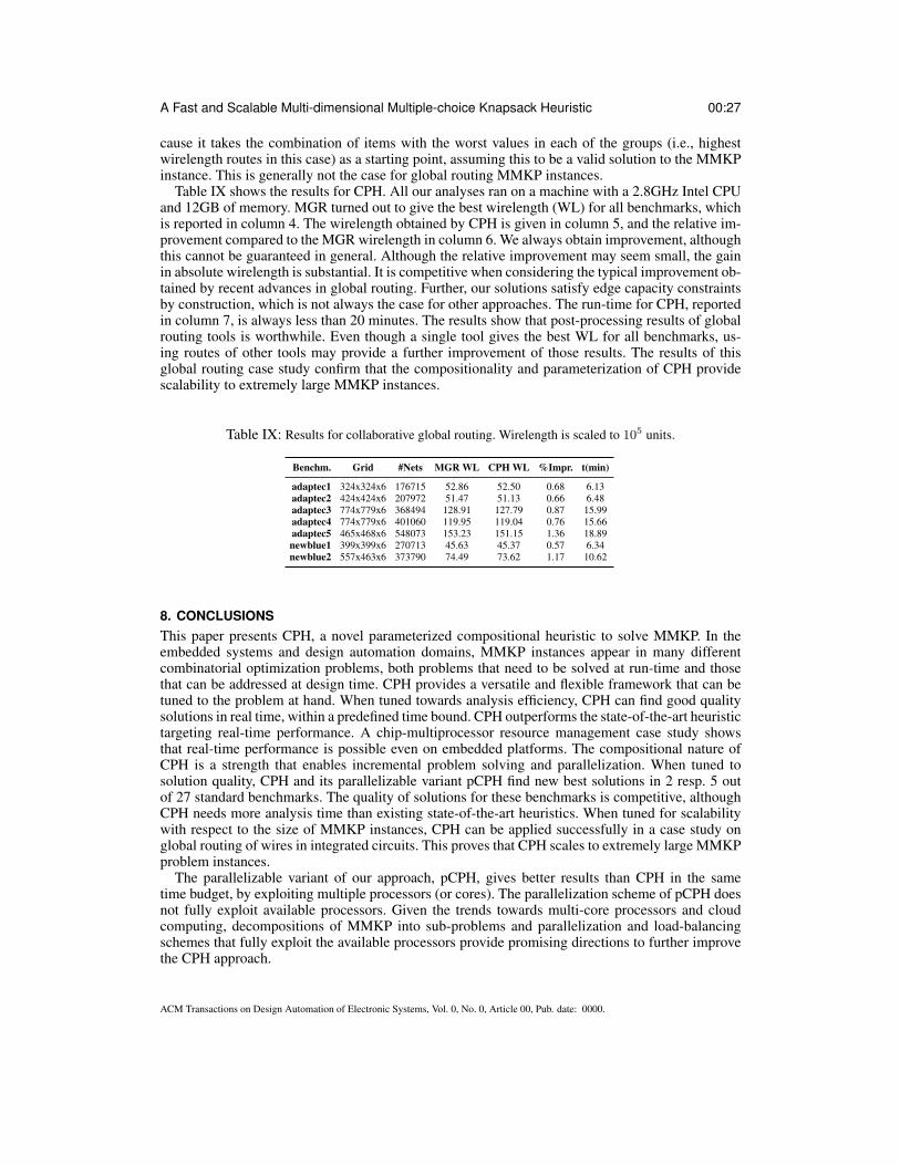
A Fast and Scalable Multi-dimensional Multiple-choice Knapsack Heuristic 00:27
cause it takes the combination of items with the worst values in each of the groups (i.e., highestwirelength routes in this case) as a starting point, assuming this to be a valid solution to the MMKPinstance. This is generally not the case for global routing MMKP instances.
Table IX shows the results for CPH. All our analyses ran on a machine with a 2.8GHz Intel CPUand 12GB of memory. MGR turned out to give the best wirelength (WL) for all benchmarks, whichis reported in column 4. The wirelength obtained by CPH is given in column 5, and the relative im-provement compared to the MGR wirelength in column 6. We always obtain improvement, althoughthis cannot be guaranteed in general. Although the relative improvement may seem small, the gainin absolute wirelength is substantial. It is competitive when considering the typical improvement ob-tained by recent advances in global routing. Further, our solutions satisfy edge capacity constraintsby construction, which is not always the case for other approaches. The run-time for CPH, reportedin column 7, is always less than 20 minutes. The results show that post-processing results of globalrouting tools is worthwhile. Even though a single tool gives the best WL for all benchmarks, us-ing routes of other tools may provide a further improvement of those results. The results of thisglobal routing case study confirm that the compositionality and parameterization of CPH providescalability to extremely large MMKP instances.
Table IX: Results for collaborative global routing. Wirelength is scaled to 105 units.
Benchm. Grid #Nets MGR WL CPH WL %Impr. t(min)
adaptec1 324x324x6 176715 52.86 52.50 0.68 6.13adaptec2 424x424x6 207972 51.47 51.13 0.66 6.48adaptec3 774x779x6 368494 128.91 127.79 0.87 15.99adaptec4 774x779x6 401060 119.95 119.04 0.76 15.66adaptec5 465x468x6 548073 153.23 151.15 1.36 18.89newblue1 399x399x6 270713 45.63 45.37 0.57 6.34newblue2 557x463x6 373790 74.49 73.62 1.17 10.62
8. CONCLUSIONSThis paper presents CPH, a novel parameterized compositional heuristic to solve MMKP. In theembedded systems and design automation domains, MMKP instances appear in many differentcombinatorial optimization problems, both problems that need to be solved at run-time and thosethat can be addressed at design time. CPH provides a versatile and flexible framework that can betuned to the problem at hand. When tuned towards analysis efficiency, CPH can find good qualitysolutions in real time, within a predefined time bound. CPH outperforms the state-of-the-art heuristictargeting real-time performance. A chip-multiprocessor resource management case study showsthat real-time performance is possible even on embedded platforms. The compositional nature ofCPH is a strength that enables incremental problem solving and parallelization. When tuned tosolution quality, CPH and its parallelizable variant pCPH find new best solutions in 2 resp. 5 outof 27 standard benchmarks. The quality of solutions for these benchmarks is competitive, althoughCPH needs more analysis time than existing state-of-the-art heuristics. When tuned for scalabilitywith respect to the size of MMKP instances, CPH can be applied successfully in a case study onglobal routing of wires in integrated circuits. This proves that CPH scales to extremely large MMKPproblem instances.
The parallelizable variant of our approach, pCPH, gives better results than CPH in the sametime budget, by exploiting multiple processors (or cores). The parallelization scheme of pCPH doesnot fully exploit available processors. Given the trends towards multi-core processors and cloudcomputing, decompositions of MMKP into sub-problems and parallelization and load-balancingschemes that fully exploit the available processors provide promising directions to further improvethe CPH approach.
ACM Transactions on Design Automation of Electronic Systems, Vol. 0, No. 0, Article 00, Pub. date: 0000.

00:28 H. Shojaei et al.
Implementations. Implementations of the algorithms presented in this paper are available throughhttp://www.es.ele.tue.nl/pareto/mmkp/.
Acknowledgement. Part of this work was supported by the EC through FP7 IST project 216224,MNEMEE. We thank the associate editor and the reviewers for their constructive feedback, whichhelped to improve the content and presentation of the paper.
REFERENCESAKBAR, M. M., RAHMAN, M. S., KAYKOBAD, M., MANNING, E. G., AND SHOJA, G. C. 2006. Solving the multidimen-
sional multiple-choice knapsack problem by constructing convex hulls. Comput. Oper. Res. 33, 5, 1259–1273.BENTLEY, J. 1980. Multidimensional divide-and-conquer. Communications of the ACM 23, 214 – 229.BORZSONYI, S., KOSSMANN, D., AND STOCKER, K. 2001. The skyline operator. In Proc. IEEE Conf. on Data Engineer-
ing. IEEE, 421–430.CHANG, Y.-J., LEE, Y.-T., AND WANG, T.-C. 2008. NTHU-Route 2.0: a fast and stable global router. In ICCAD. 338–343.CHERFI, N. 2009. Hybrid algorithms for knapsack problems. Ph.D. thesis, University of Paris I, France.CHERFI, N. AND HIFI, M. 2008. A column generation method for the multiple-choice multi-dimensional knapsack problem.
Comput. Optim. Appl. 46, 1, 51–73.CHERFI, N. AND HIFI, M. 2009. Hybrid algorithms for the multiple-choice multi-dimensional knapsack problem. Int. J.
Operational Research 5, 1, 89–109.Cplex 2012. IBM ILOG Cplex. http://www-01.ibm.com/software/websphere/ products/optimization/academic-initiative/.CREVITS, I., HANAFI, S., MANSI, R., AND WILBAUT, C. 2012. Iterative semi-continuous relaxation heuristics for the
multiple-choice multidimensional knapsack problem. Computers & Operations Research 39, 32 – 41.DAI, K.-R., LIU, W.-H., AND LI, Y.-L. 2012. NCTU-GR: Efficient simulated evolution-based rerouting and congestion-
relaxed layer assignment on 3-d global routing. IEEE Trans. on Very Large Scale Integration (VLSI) Systems 20, 3,459–472.
GEILEN, M. AND BASTEN, T. 2007. A calculator for Pareto points. In Proc. DATE. IEEE, 285–290.GEILEN, M., BASTEN, T., THEELEN, B. D., AND OTTEN, R. 2005. An algebra of Pareto points. In Proc. ACSD. IEEE,
88–97.GEILEN, M., BASTEN, T., THEELEN, B. D., AND OTTEN, R. 2007. An algebra of Pareto points. Fundamenta Informati-
cae 78, 1, 35–74.GODFREY, P., SHIPLEY, R., AND GRYZ, J. 2005. Maximal vector computation in large data sets. In Proc. 31st Int. Conf. on
VLDB. VLDB Endowment, 229–240.HANAFI, S., MANSI, R., AND WILBAUT, C. 2009. Iterative relaxation-based heuristics for the multiple-choice multidimen-
sional knapsack problem. LNCS 5818, 73–83.HIFI, M., MICHRAFY, M., AND SBIHI, A. 2004. Heuristic algorithms for the multiple-choice multidimensional knapsack
problem. Operational Research Society 55, 12, 1323–1332.HIFI, M., MICHRAFY, M., AND SBIHI, A. 2006. A reactive local search-based algorithm for the multiple-choice multi-
dimensional knapsack problem. Comput. Optim. Appl. 33, 2-3, 271–285.HIREMATH, C. S. AND HILL, R. R. 2007. New greedy heuristics for the multiple-choice multi-dimensional knapsack
problem. Int. J. Operational Research 2, 4, 495–512.HU, J., ROY, J., AND MARKOV, I. 2010. Completing high-quality global routes. In Intl Symp. on Physical Design, Proc.
ACM, 35–41.ISPD CONTESTS 2007,. 2008. http://www.ispd.cc/contests/.KHAN, S. 1998. Quality adaptation in a multisession multimedia system: Model, algorithms and architecture. Ph.D. thesis,
Univ. of Victoria, Victoria, B.C., Canada.KHAN, S., LI, K. F., MANNING, E. G., AND AKBAR, M. M. 2002. Solving the knapsack problem for adaptive multimedia
systems. Stud. Inform. Univ. 2, 1, 157–178.KUNG, H., LUCCIO, F., AND PREPARATA, F. 1975. On finding the maxima of a set of vectors. Journal of the ACM 22, 469
– 476.MMKP benchmarks 2010. MMKP benchmarks. ftp://cermsem.univ-paris1.fr/pub/CERMSEM/hifi/MMKP/MMKP.html.MMKP benchmarks 2012. MMKP benchmarks. http://www.es.ele.tue.nl/pareto/mmkp/.MOSER, M., JOKANOVIC, D. P., AND SHIRATORI, N. 1997. An algorithm for the multidimensional multiple-choice knap-
sack problem. IEICE Trans. Fund. Electron. Comm. Comput. Sci. 80, 3, 582–589.PARRA-HERNANDEZ, R. AND DIMOPOULOS, N. J. 2005. A new heuristic for solving the multichoice multidimensional
knapsack problem. IEEE Trans. on Systems, Man, and Cybernetics A 35, 5, 708–717.PISINGER, D. 1995. Algorithms for knapsack problems. Ph.D. thesis, DIKU, University of Copenhagen, Denmark.
ACM Transactions on Design Automation of Electronic Systems, Vol. 0, No. 0, Article 00, Pub. date: 0000.

A Fast and Scalable Multi-dimensional Multiple-choice Knapsack Heuristic 00:29
PREPARATA, F. AND SHAMOS, M. 1985. Computational Geometry – An Introduction. Springer.SBIHI, A. 2003. Hybrid methods in combinatorial optimization: Exact algorithms and heuristics. Ph.D. thesis, Univ. of Paris
I, France.SBIHI, A. 2007. A best first search exact algorithm for the multiple-choice multidimensional knapsack problem. J. Comb.
Optim. 13, 4, 337–351.SHOJAEI, H., GHAMARIAN, A., BASTEN, T., GEILEN, M., STUIJK, S., AND HOES, R. 2009. A parameterized compo-
sitional multi-dimensional multiple-choice knapsack heuristic for CMP run-time management. In Proc. DAC. ACM,917–922.
SHOJAEI, H., WU, T.-H., DAVOODI, A., AND BASTEN, T. 2010. A Pareto-algebraic framework for signal power optimiza-tion in global routing. In Proc. ISLPED, ACM. 407–412.
SimIt-ARM 2012. SimIt-ARM. http://simit-arm.sourceforge.net.XU, Y. AND CHU, C. 2011. MGR: Multi-level global router. In Proc. ICCAD. IEEE, 250–255.XU, Y., ZHANG, Y., AND CHU, C. 2009. Fastroute 4.0: global router with efficient via minimization. In ASP-DAC. 576–581.YKMAN-COUVREUR, C., NOLLET, V., CATTHOOR, F., AND CORPORAAL, H. 2011. Fast multidimension multichoice
knapsack heuristic for MP-SoC runtime management. ACM Trans. on Embedded Computing Systems 10, 3, Art. 35.YKMAN-COUVREUR, C., NOLLET, V., MARESCAUX, T., BROCKMEYER, E., CATTHOOR, F., AND CORPORAAL, H.
2006. Fast multi-dimension multi-choice knapsack heuristic for MP-SoC run-time management. In Proc. ISSOC. IEEE,1–4.
YUKISH, M. 2004. Algorithms to identify Pareto points in multi-dimensional data sets. Ph.D. thesis, Pennsylvania StateUniversity.
ACM Transactions on Design Automation of Electronic Systems, Vol. 0, No. 0, Article 00, Pub. date: 0000.