0-3-DIAGNOSTICSANDPROGNOSTICS - Lund … document/5373_full...0-3-DIAGNOSTICSANDPROGNOSTICS...

Indust

rial E

lectr

ical Engin

eering a

nd A

uto

mation

CODEN:LUTEDX/(TEIE-5373)/1-65/(2016)

PMSM diagnostics and prognostics Evaluation of an on-line method based onhigh frequency current response

Julius Björngreen

Division of Industrial Electrical Engineering and Automation Faculty of Engineering, Lund University

Master Thesis

PMSM diagnostics and prognostics

Evaluation of an on-line method based on

high frequency current response

Julius Björngreen

Supervisor (Volvo AB) Zhe HuangSupervisor (LTH) Avo Reinap

Examiner (LTH) Mats Alaküla

Master Thesis in Industrial Electrical Engineering and AutomationDivision of Electrical Engineering

Department of Biomedical EngineeringFaculty of Engineering - Lund University

Abstract

This thesis covers and evaluates a stator insulation fault detection method forPermanent Magnetised Synchronous Machines (PMSMs). The method could beimplemented on-line and is based on using the power converter in an electric orhybrid vehicle to measure the State of Health (SoH) of the stator insulation ofthe PMSM. This is done through measurements of the high frequency currentresponse that occurs when the PMSM is subjected to a voltage pulse from thepower converter. The high frequency content of this current response is relatedto the parasitic capacitances of the PMSM and thereby also reflect the quality ofthe stator insulation. It is shown, in this thesis, that small impedance changes,corresponding to degradation and an early developing fault, can be detected withhigh repeatability and accuracy.

ii

Acknowledgements

My first thanks goes to Zhe Huang, my supervisor from Volvo, who came up withthe idea for this thesis and provided great discussions and regular contact duringthe whole thesis project. Secondly I thank my supervisor from LTH, AssociateProfessor Avo Reinap, who always found the time to discuss issues and provideadvice. I also thank my examiner Professor Mats Alaküla for all valuable inputand advice. A large thank you goes to Sebastian Hall who above all helped mea lot with the LabView programming of the CompactRIO system for the motorcontrol. Sebastian also deserve a great thanks for all his tips and all productivediscussions with bouncing of ideas and so on. A big thanks also goes to GetachewDarge, the committed enthusiast, who provides, keeps track of and maintains allinstruments, equipment and tools. He was of great help especially, but far fromonly, when the test rig with the electric machine was set up when cables, specifictools and advice on good practical solutions were needed.

iii

List of Abbreviations

AC Alternating Current

AD Analogue to Digital

ADC Analogue to Digital Converter

cRIO Compact Reconfigurable Input Output

CSA Current Signature Analysis

DC Direct Current

EV Electric Vehicle

FEM Finite Element Method

FFT Fast Fourier Transform

FPGA Field-Programmable Gate Array

IEEE Institute of Electrical and Electronics Engineers

IGBT Insulated-Gate Bipolar Transistor

IM Induction Motor

LTH Faculty of Engineering - Lund University

MS\s Mega Samples per second

n\a not available

PD-test Partial Discharge Test

PMSM Permanent Magnetised Synchronous Machine

PWM Pulse Width Modulated

RAM Random Access Memory

rpm revolutions per minute

SoH State of Health

VSC Voltage Source Converter

iv

List of Figures

2.1 Principal drawing of the stator of a PMSM or particularly thePMSM most used during the experiments conducted during thismaster thesis (H5M1). This machine has 24 slots (only six drawnhere). The windings are so called random wound and every windingcontains eight round turns. Every slot contains two windings fromdifferent phases that are separated by a slot divider. . . . . . . . . 8

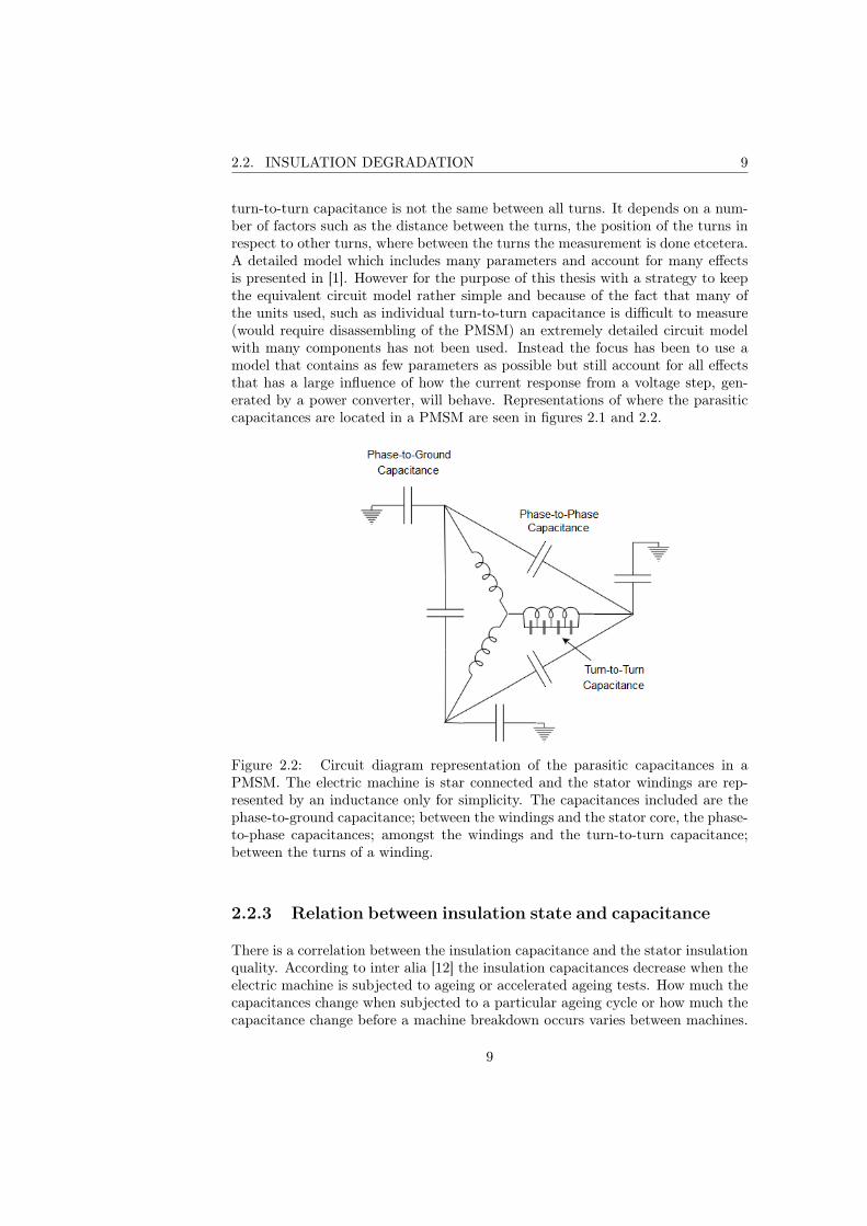
2.2 Circuit diagram representation of the parasitic capacitances in aPMSM. The electric machine is star connected and the stator wind-ings are represented by an inductance only for simplicity. The ca-pacitances included are the phase-to-ground capacitance; betweenthe windings and the stator core, the phase-to-phase capacitances;amongst the windings and the turn-to-turn capacitance; betweenthe turns of a winding. . . . . . . . . . . . . . . . . . . . . . . . . 9

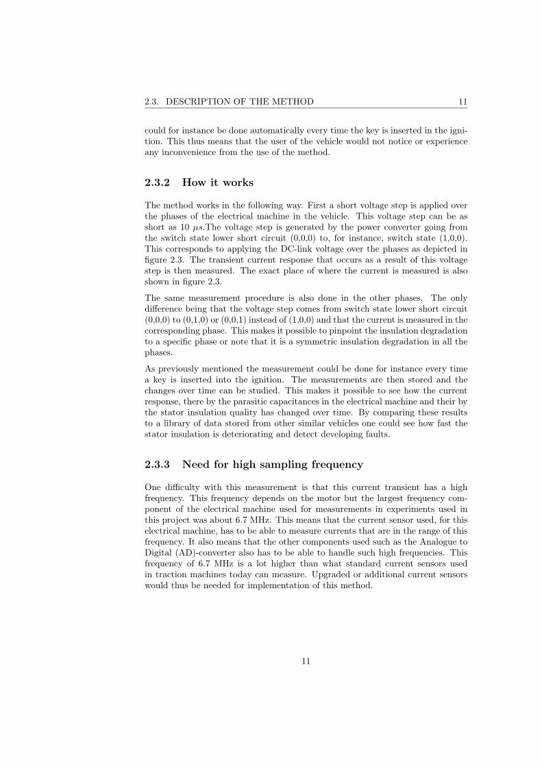
2.3 Illustration of where a voltage step is applied in the electrical ma-chine. To the left is a representation of the status of the switches(transistors) in the power converter when a voltage step is gener-ated. The left picture also includes how the electrical machine’swindings are connected to the power converter and where the cur-rent is measured. The right circuit is equivalent with the left andshows the result of setting the switches as in the left picture. . . . 12

3.1 Segment of the stator from a Finite Element Method (FEM)-modelof the electrical machine used. Three slots are seen on this segmentwhich is an eighth on the stator (24 slots in total). Every slotcontains two coils from different phases (not seen in the picture). . 14

3.2 Equivalent circuit model of the electrical machine under test. Notseen in this picture is the mutual inductive coupling factor betweenthe phase windings. Also not seen in the picture are the seriesresistance of the winding inductances. . . . . . . . . . . . . . . . . 15

3.3 Current response from the simulation model without any simulatedfault. The green curve is the current and the blue one is the voltage. 17

4.1 Block diagram of the test set-up. . . . . . . . . . . . . . . . . . . 204.2 Picture of the PMSM under test. . . . . . . . . . . . . . . . . . . . 21

v

LIST OF FIGURES LIST OF FIGURES

5.1 Current responses from a 50 V voltage step with a pulse width of 10µs. The current is measured in phase U. The graph is constructedfrom mean values of ten measurements. Notice the high frequencyoscillations in the beginning of the response that later rings out andthe graph turns into a curve increasing with a constant derivative. 26

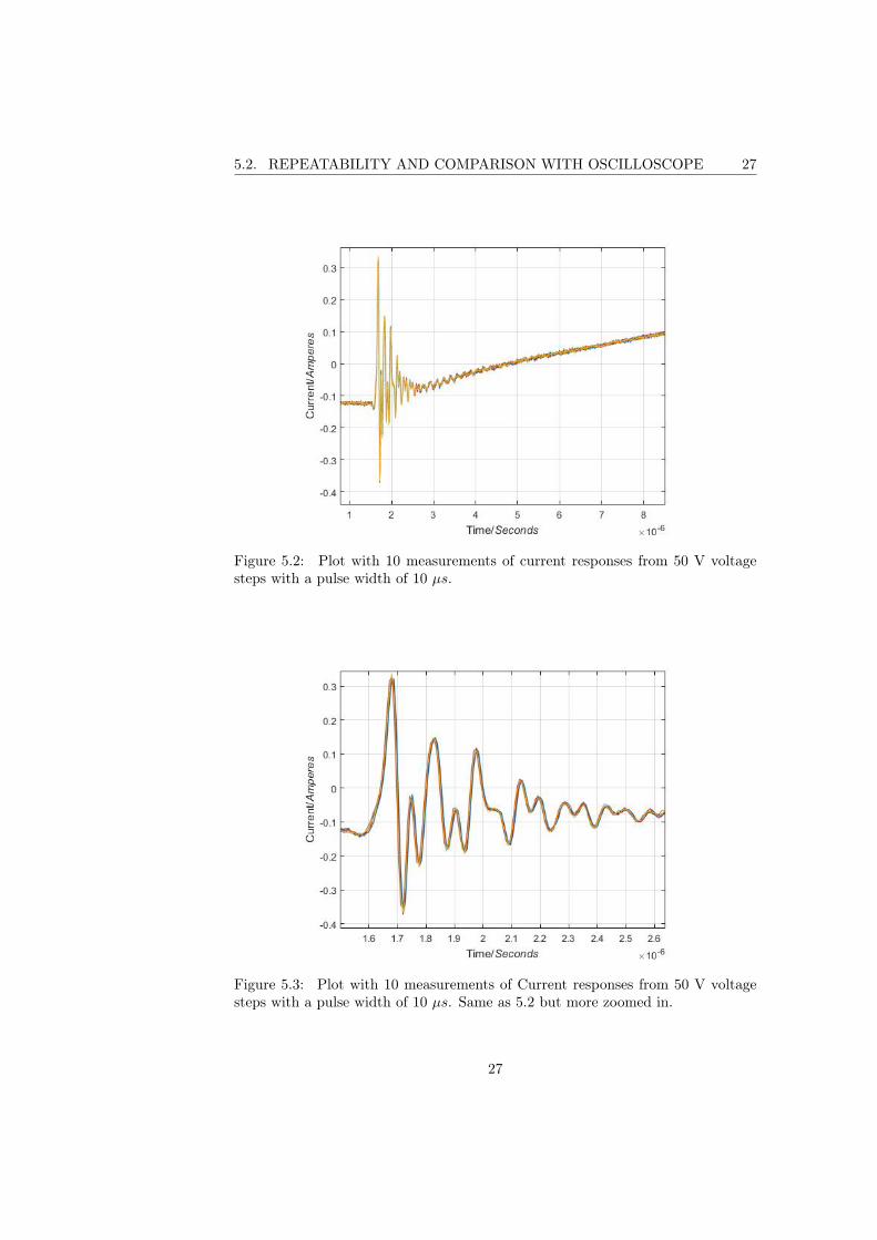
5.2 Plot with 10 measurements of current responses from 50 V voltagesteps with a pulse width of 10 µs. . . . . . . . . . . . . . . . . . . 27

5.3 Plot with 10 measurements of Current responses from 50 V voltagesteps with a pulse width of 10 µs. Same as 5.2 but more zoomed in. 27

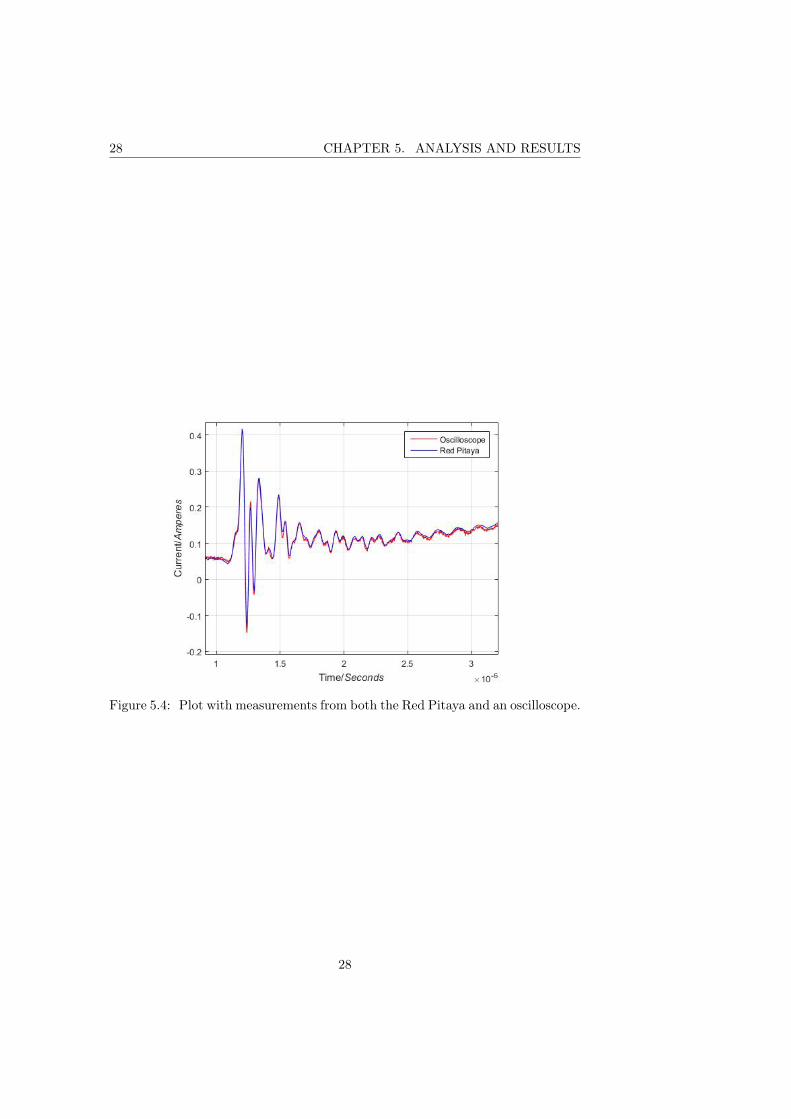
5.4 Plot with measurements from both the Red Pitaya and an oscilloscope. 285.5 Current responses from measurements with four different rotor po-

sitions. Notice the difference mainly seen to the right in the plot.. . . . . . . . . . . . . . . . . . . . . . . . . . . . . . . . . . . . . . 29

5.6 Current responses from measurements with four different rotor po-sitions after the subtraction of the constant current derivative. No-tice that the earlier difference between the for curves, seen in figure5.5,now is difficult to observe at all. . . . . . . . . . . . . . . . . . 30

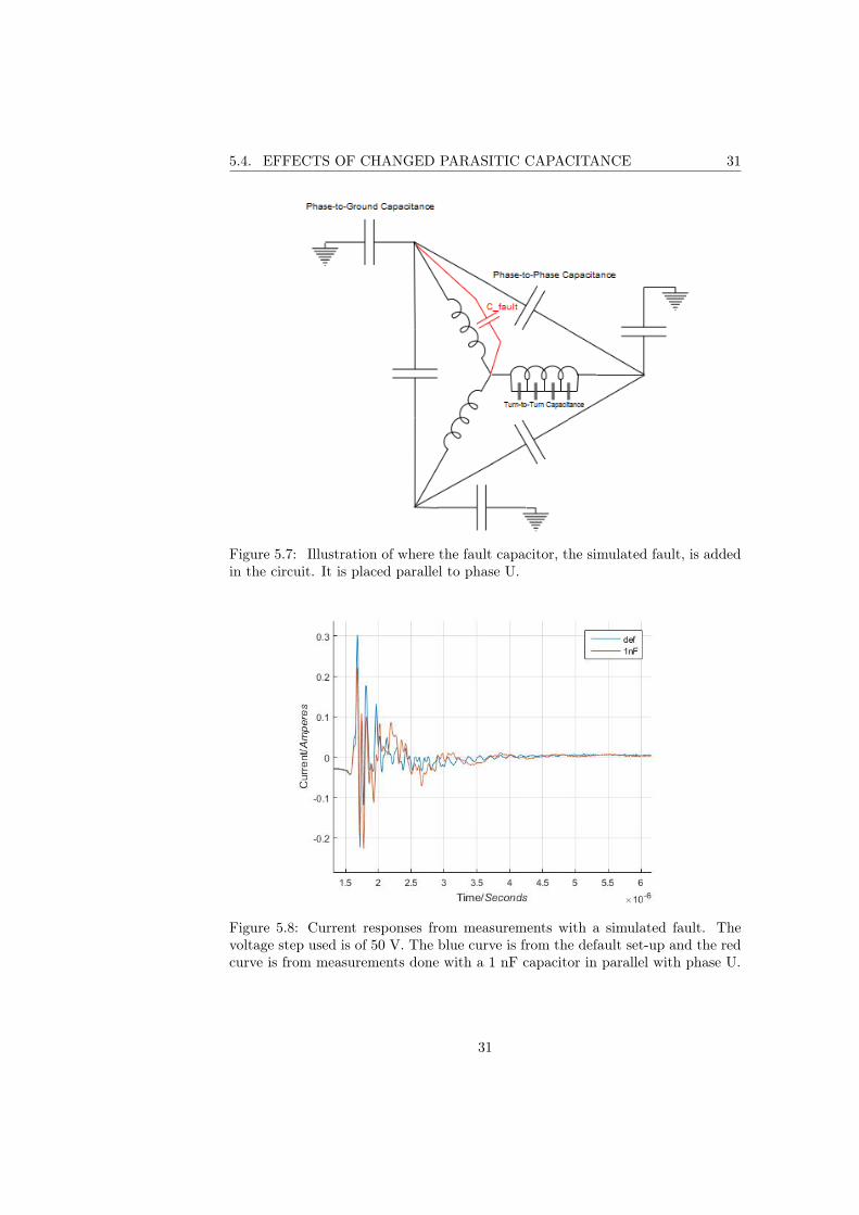
5.7 Illustration of where the fault capacitor, the simulated fault, isadded in the circuit. It is placed parallel to phase U. . . . . . . . . 31

5.8 Current responses from measurements with a simulated fault. Thevoltage step used is of 50 V. The blue curve is from the defaultset-up and the red curve is from measurements done with a 1 nFcapacitor in parallel with phase U. . . . . . . . . . . . . . . . . . . 31

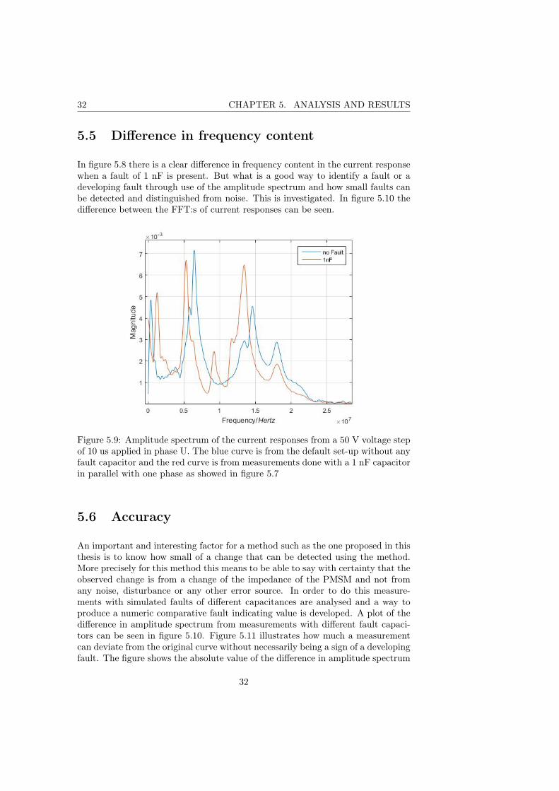
5.9 Amplitude spectrum of the current responses from a 50 V voltagestep of 10 us applied in phase U. The blue curve is from the defaultset-up without any fault capacitor and the red curve is from mea-surements done with a 1 nF capacitor in parallel with one phase asshowed in figure 5.7 . . . . . . . . . . . . . . . . . . . . . . . . . . 32

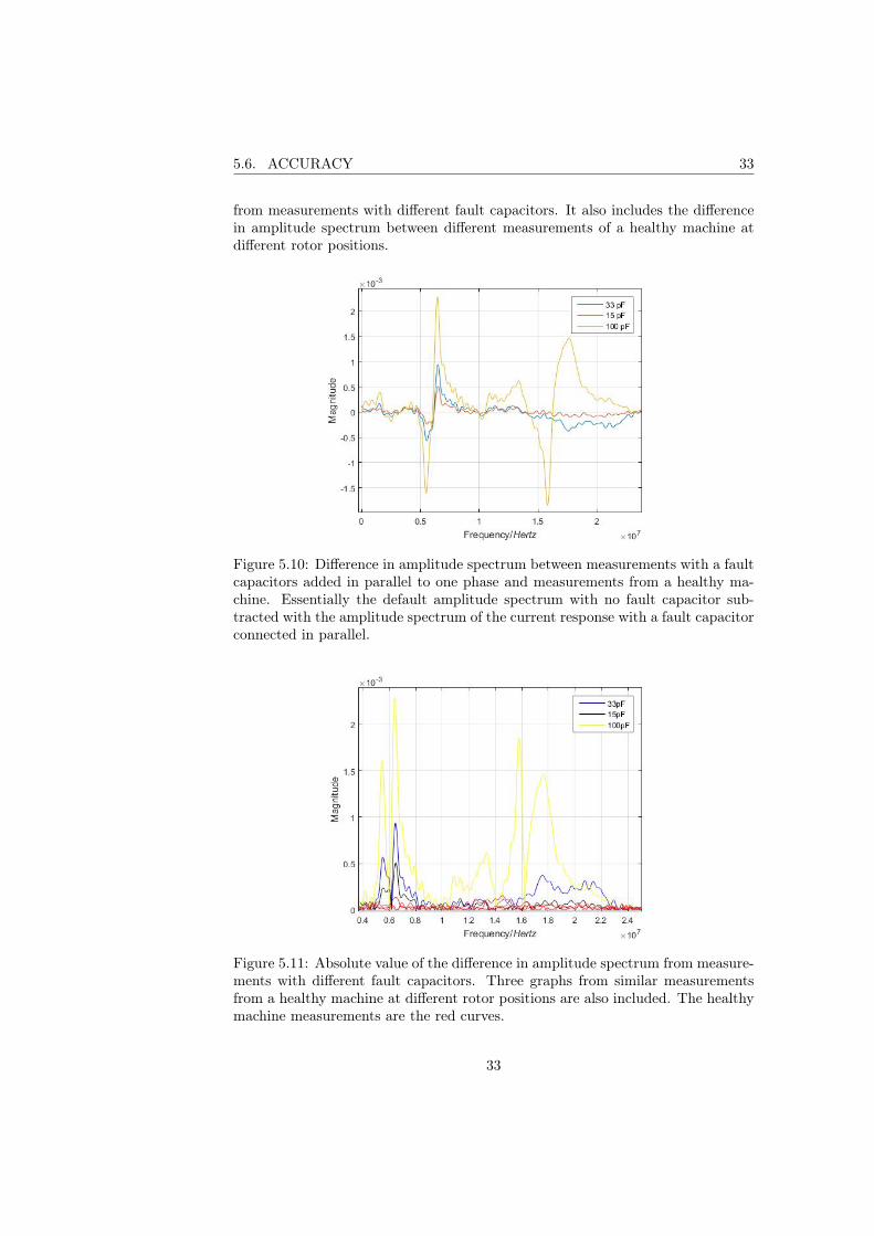
5.10 Difference in amplitude spectrum between measurements with afault capacitors added in parallel to one phase and measurementsfrom a healthy machine. Essentially the default amplitude spectrumwith no fault capacitor subtracted with the amplitude spectrum ofthe current response with a fault capacitor connected in parallel. . 33

5.11 Absolute value of the difference in amplitude spectrum from mea-surements with different fault capacitors. Three graphs from similarmeasurements from a healthy machine at different rotor positionsare also included. The healthy machine measurements are the redcurves. . . . . . . . . . . . . . . . . . . . . . . . . . . . . . . . . . . 33

5.12 High frequency current response right before the electric machine(usual) and right after the power converter (cabinet). The wordcabinet refers to that the current probe was placed inside the cab-inet containing the power converter etcetera. In the plot there aremeasurements from two series of measurements from the cabinet. . 36

5.13 Amplitude spectrum of the current response right before the electricmachine (usual) and right after the power converter (cabinet). . . 36

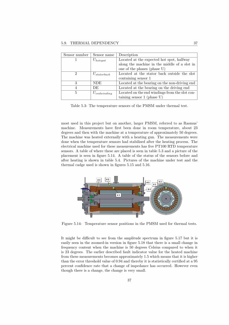
5.14 Temperature sensor positions in the PMSM used for thermal tests. 37

vi


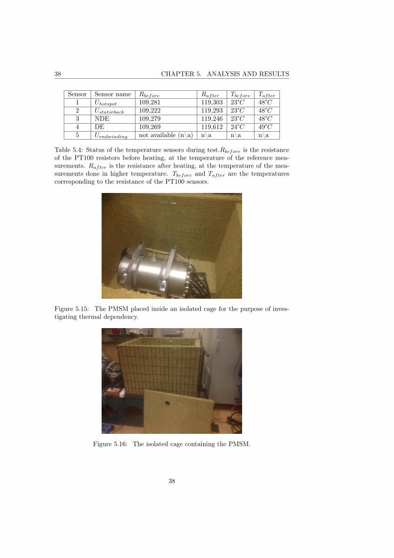
5.15 The PMSM placed inside an isolated cage for the purpose of inves-tigating thermal dependency. . . . . . . . . . . . . . . . . . . . . . 38

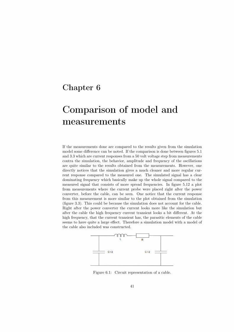
5.16 The isolated cage containing the PMSM. . . . . . . . . . . . . . . 385.17 Amplitude spectrum from measurements in room temperature and

at approximately 50 degrees Celsius. . . . . . . . . . . . . . . . . 395.18 Amplitude spectrum from measurements in room temperature and

at approximately 50 degrees Celsius, zoomed in. . . . . . . . . . . 39

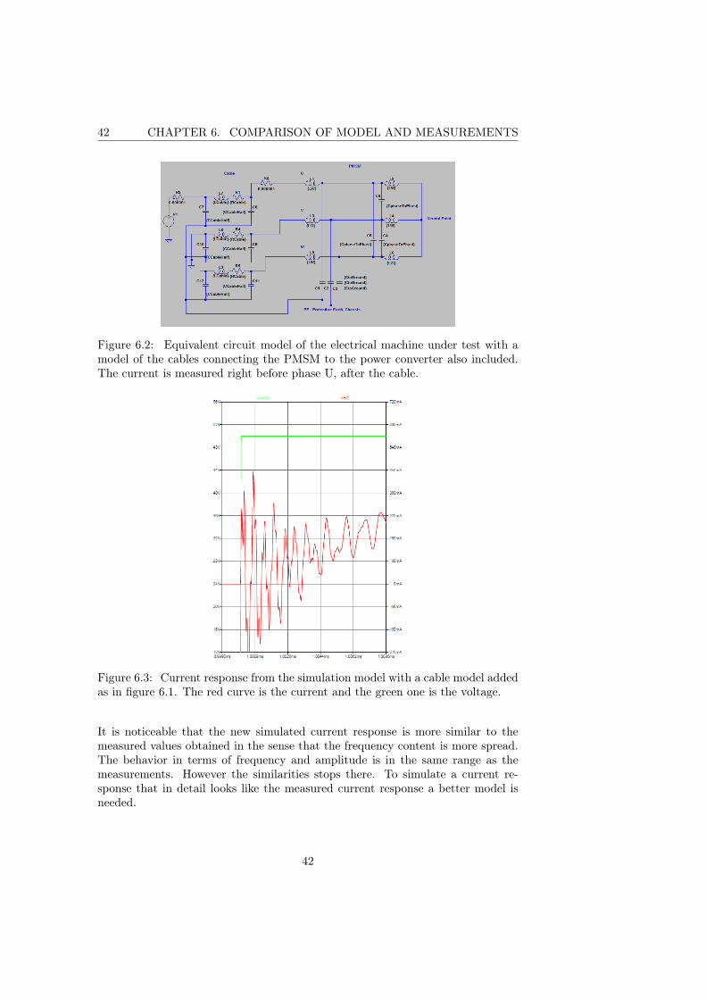
6.1 Circuit representation of a cable. . . . . . . . . . . . . . . . . . . . 416.2 Equivalent circuit model of the electrical machine under test with

a model of the cables connecting the PMSM to the power converteralso included. The current is measured right before phase U, afterthe cable. . . . . . . . . . . . . . . . . . . . . . . . . . . . . . . . . 42

6.3 Current response from the simulation model with a cable modeladded as in figure 6.1. The red curve is the current and the greenone is the voltage. . . . . . . . . . . . . . . . . . . . . . . . . . . . 42

vii


viii

List of Tables

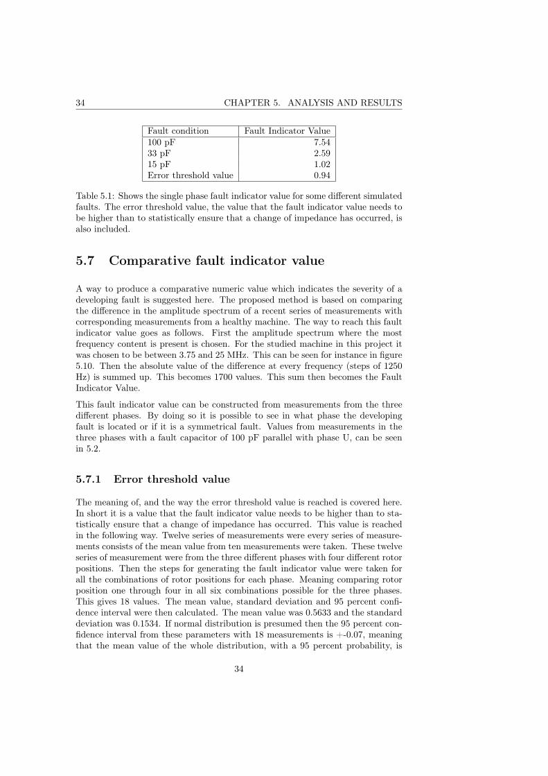
5.1 Shows the single phase fault indicator value for some different sim-ulated faults. The error threshold value, the value that the faultindicator value needs to be higher than to statistically ensure thata change of impedance has occurred, is also included. . . . . . . . . 34

5.2 Shows the Fault Indicator Value from measurements from the threedifferent phases from a simulated fault of 100 pF parallel to phase U. 35

5.3 The temperature sensors of the PMSM under thermal test. . . . . 375.4 Status of the temperature sensors during test.Rbefore is the resis-

tance of the PT100 resistors before heating, at the temperature ofthe reference measurements. Rafter is the resistance after heating,at the temperature of the measurements done in higher tempera-ture. Tbefore and Tafter are the temperatures corresponding to theresistance of the PT100 sensors. . . . . . . . . . . . . . . . . . . . 38

ix

LIST OF TABLES LIST OF TABLES

x

Contents

Abstract . . . . . . . . . . . . . . . . . . . . . . . . . . . . . . . . . . . iiAcknowledgements . . . . . . . . . . . . . . . . . . . . . . . . . . . . iiiList of Abbreviations . . . . . . . . . . . . . . . . . . . . . . . . . . . ivList of Figures . . . . . . . . . . . . . . . . . . . . . . . . . . . . . . . viiList of Tables . . . . . . . . . . . . . . . . . . . . . . . . . . . . . . . . ix

1 Introduction 11.1 Background . . . . . . . . . . . . . . . . . . . . . . . . . . . . . . . 11.2 Disposition . . . . . . . . . . . . . . . . . . . . . . . . . . . . . . . 21.3 Working methodology . . . . . . . . . . . . . . . . . . . . . . . . . 21.4 Previous Work . . . . . . . . . . . . . . . . . . . . . . . . . . . . . 3

1.4.1 Today existing diagnostic methods . . . . . . . . . . . . . . 31.4.2 On-line diagnostic methods . . . . . . . . . . . . . . . . . . 4

1.5 Purpose . . . . . . . . . . . . . . . . . . . . . . . . . . . . . . . . . 41.6 Delimitations . . . . . . . . . . . . . . . . . . . . . . . . . . . . . . 4

2 Method description and theory 52.1 Theory . . . . . . . . . . . . . . . . . . . . . . . . . . . . . . . . . . 5

2.1.1 Inverter fed electrical machines . . . . . . . . . . . . . . . . 52.1.2 Stator of an electrical machine . . . . . . . . . . . . . . . . 62.1.3 Stator insulation . . . . . . . . . . . . . . . . . . . . . . . . 6

2.2 Insulation degradation . . . . . . . . . . . . . . . . . . . . . . . . . 72.2.1 Parasitic capacitance . . . . . . . . . . . . . . . . . . . . . . 82.2.2 Parasitic capacitances in a PMSM . . . . . . . . . . . . . . 82.2.3 Relation between insulation state and capacitance . . . . . 92.2.4 Equations . . . . . . . . . . . . . . . . . . . . . . . . . . . . 10

2.3 Description of the Method . . . . . . . . . . . . . . . . . . . . . . . 102.3.1 Idea . . . . . . . . . . . . . . . . . . . . . . . . . . . . . . . 102.3.2 How it works . . . . . . . . . . . . . . . . . . . . . . . . . . 112.3.3 Need for high sampling frequency . . . . . . . . . . . . . . . 11

3 Electrical model 133.1 Construction of equivalent circuit . . . . . . . . . . . . . . . . . . . 13

3.1.1 Parasitic capacitance calculation . . . . . . . . . . . . . . . 133.1.2 Description of the model . . . . . . . . . . . . . . . . . . . . 153.1.3 Mutual Inductance . . . . . . . . . . . . . . . . . . . . . . . 16

xi

CONTENTS CONTENTS

3.2 Simulated current response . . . . . . . . . . . . . . . . . . . . . . 17

4 Experimental Procedure 194.1 Implementation . . . . . . . . . . . . . . . . . . . . . . . . . . . . . 19

4.1.1 Test Set-up . . . . . . . . . . . . . . . . . . . . . . . . . . . 194.1.2 Test object 1 . . . . . . . . . . . . . . . . . . . . . . . . . . 204.1.3 Test object 2 . . . . . . . . . . . . . . . . . . . . . . . . . . 204.1.4 Motor Control . . . . . . . . . . . . . . . . . . . . . . . . . 204.1.5 Current measurement . . . . . . . . . . . . . . . . . . . . . 214.1.6 Data logging . . . . . . . . . . . . . . . . . . . . . . . . . . 224.1.7 Equipment used . . . . . . . . . . . . . . . . . . . . . . . . 224.1.8 Performed tests . . . . . . . . . . . . . . . . . . . . . . . . . 22

4.2 Data Analysis . . . . . . . . . . . . . . . . . . . . . . . . . . . . . . 23

5 Analysis and results 255.1 Characteristics of the current response . . . . . . . . . . . . . . . . 255.2 Repeatability and comparison with oscilloscope . . . . . . . . . . . 265.3 Rotor position dependency . . . . . . . . . . . . . . . . . . . . . . 295.4 Effects of changed parasitic capacitance . . . . . . . . . . . . . . . 305.5 Difference in frequency content . . . . . . . . . . . . . . . . . . . . 325.6 Accuracy . . . . . . . . . . . . . . . . . . . . . . . . . . . . . . . . 325.7 Comparative fault indicator value . . . . . . . . . . . . . . . . . . . 34

5.7.1 Error threshold value . . . . . . . . . . . . . . . . . . . . . 345.8 Influence of current sensor location . . . . . . . . . . . . . . . . . . 355.9 Thermal dependency . . . . . . . . . . . . . . . . . . . . . . . . . . 36

5.9.1 Larger machine . . . . . . . . . . . . . . . . . . . . . . . . . 39

6 Comparison of model and measurements 41

7 Conclusion and future work 437.1 Conclusion . . . . . . . . . . . . . . . . . . . . . . . . . . . . . . . 43

7.1.1 Hardware requirements . . . . . . . . . . . . . . . . . . . . 447.2 Suggestions for Future work . . . . . . . . . . . . . . . . . . . . . . 44

7.2.1 More extensive testing . . . . . . . . . . . . . . . . . . . . . 447.2.2 Better electrical model . . . . . . . . . . . . . . . . . . . . . 44

References 45Appendix A, Winding inductance and capacitance measure-

ments with LCR-meter . . . . . . . . . . . . . . . . . . . . . . . 47

xii

Chapter 1

Introduction

1.1 Background

Electrical machines are generally highly reliable. However, the electrical machinethat acts as motor or generator in Electric Vehicles (EVs) is used at different,much more varied, load conditions compared to a traditional electrical machinein a factory. The operation of the EV is often such that the electrical machine init is used at quickly altered load conditions and is subjected to multiple stressessuch as thermal, mechanical and ambient stresses. The fast switching of modernpower electronics such as Insulated-Gate Bipolar Transistors (IGBTs) in the powerconverter also puts further stress on the electrical machine. The electrical machinein EVs is also required to provide as high power density as possible in order toget a high return on investment. Since the weight and size of the electric machineis designed to be as small as possible, while still maintaining its function, theelectrical machine is often used near its rated values. This includes both the ratedvalues for continuous as well as peak torque and power. At the same time theEV is required to deliver high up-time and an unscheduled stop of a machine isunacceptable and is associated with large economic losses and safety issues.

With this in mind a reliable method for monitoring the SoH of electrical machineswould be of great interest in this aspect. If a fault can be detected before it occursit would certainly be beneficial compared to detecting it by noticing the machinenot working. It would also be beneficial if this monitoring could be done on linewithout needing to take the vehicle to a workshop or disconnect the electricalmachine.

A critical aspect of electric traction motor drives is the stator insulation system.According to different studies stator winding insulation failures account for abouta third of all electric motor failures. In particular the most comprehensive studydone on the subject, that surveyed 7500 large Induction Motors (IMs), found that37 % of all failures were related to stator winding problems[10][p131]. For thisreason, monitoring of the stator insulation is deemed highly interesting.

1

2 CHAPTER 1. INTRODUCTION

The stator insulation is subjected to mechanical, thermal, ambient and electricalstresses and the lifetime of the stator depends heavily on how much it is subjectedto these stresses. The degradation of the stator insulation is often a slow process.However, as the stator insulation deteriorates, the parasitic insulation capacitanceschange [7][9]. An ability to monitor the parasitic capacitances, namely the phase-to-phase, phase-to-core and turn-to-turn capacitances of the electrical machine,would consequentially result in an ability to be able to detect degradation of thestator insulation. The method proposed in this thesis relies on measuring thesecapacitances indirectly from measuring the high frequency current response thatappears when a voltage step is applied over the motor windings.

1.2 Disposition

Below follows a list that gives a short introduction to the content of all chaptersin this thesis.

• Chapter 1, Introduction, gives a background and motivation to the proposedfault detection technique and presents previous work.

• Chapter 2, Method description and theory, explains the proposed fault de-tection method and the relevant theory behind it.

• Chapter 3, Electrical model, presents a simulation model that has been de-veloped in order to simulate the proposed method in Lt-SPICE.

• Chapter 4, Experimental procedure , presents how the tests and experimentswere carried out, the experimental set-up and equipment that was used.

• Chapter 5, Analysis and results, goes through the results, the post processingof data, the accuracy of the measurements and addresses how to interpretthe data.

• Chapter 6, Comparison of model and measurements, compares the experi-mental results obtained with the simulated results gathered from the elec-trical model.

• Chapter 7, Conclusion and future work, concludes the thesis and suggestsfuture work.

1.3 Working methodology

The working methodology used during this master thesis project is divided intophases. These phases are listed and shortly described below:

• After a goal document and a project plan were approved this master the-sis project started with a literature study. The literature studied consistsof presented articles that address fault detection techniques and diagnosticsmethods for electrical machines. The literature study also includes reading

2

1.4. PREVIOUS WORK 3

up on relevant theory.

• Phase two of this master thesis project consists of making measurements onthe PMSM tested during this project with lab equipment such as impedanceanalyser, oscilloscope etcetera. The purpose of these measurements were tobe a basis for the construction of an equivalent circuit model of the test ob-ject in LtSPICE. These measurements also provided basis for the choosingof what components to use for the construction of the measuring equipment.This phase also include programming of the motor control software in Lab-view.

• The third phase consists of building and programming the equipment usedfor making measurements. The programming of the Red Pitaya that is usedfor making and storing the measurements are written in MATLAB.

• The fourth phase includes the actual measuring and the analysis of the mea-sured data. Lots of different measurements under different conditions aremade and the data analysis is done in MATLAB. After the data analysisa comparison between the obtained measurement results and the LtSPICEsimulation model is done. This is followed by evaluation and improvementof the simulation model.

• The fifth and last phase consists of writing the final report. This was tosome extent done in parallel with earlier phases, especially the data analysisphase, but most of the report writing is done last when all data was gatheredand analysed.

1.4 Previous Work

1.4.1 Today existing diagnostic methods

On the market today there are some methods for determining the SoH of an electri-cal machine. However the methods that are used today are often either expensiveor require disconnection of the motor and thus has to be done in a workshop.Methods like these that require out-take and/or has to be done in a workshopare called off-line methods. According to [14] most of the industrially acceptedtest are off-line fault detection methods and include the off-line surge test, theDirect Current (DC)-conductivity test, the insulation resistance test,polarisationindex and the DC/AC HIPot test [14]. Those methods are as stated off-line meth-ods and if possible an on-line method would certainly be preferable to an off-linemethod since less or no intervention is needed in an on-line method. An indus-trially accepted on-line test is the Partial Discharge Test (PD-test). This test

3

4 CHAPTER 1. INTRODUCTION

unfortunately also has disadvantages. One of them is that the method requiresexpensive measurement equipment.

1.4.2 On-line diagnostic methods

There are some on-line fault detection techniques that have been presented but notconsidered industrially accepted. A selection of these are: a method for detectingturn faults through Current Signature Analysis (CSA) investigated in [5], an on-line version of the Surge Test investigated in [4] and a method which involvesmeasuring and evaluating the leakage current between connector and ground todetermine phase-to-ground insulation, presented in [13]. These methods are notdiscussed further in this thesis but are all available on the web at Institute ofElectrical and Electronics Engineers (IEEE)-explorer which is IEEEs database forpublished articles and writings.

Different authors have published articles where the test methods are quite similarto the one proposed in this thesis. All of the methods presented however, that I,the author of this thesis have found, are made on IMs. In this thesis the proposedmethod is instead applied on a PMSM. In [14] experiments somewhat similar tothe ones made in this thesis on a PMSM are done on a 5.5 kW, 2-pole, squirrel-cageinduction machine.

1.5 Purpose

The purpose of this master thesis project is to evaluate the proposed fault detec-tion method and determine if the method can be implemented on a PMSM. Thework includes making experimental tests and modelling in a simulation program(LtSPICE). The work will also include an investigation on what the minimumhardware requirements would be for implementing the method in a vehicle. Theequipment in a vehicle today is most likely too slow to be able to make the mea-surements required. However the development of this equipment goes forward andthe costs get lower. In the future there could be a high possibility that this methodis deemed economically viable.

1.6 Delimitations

This thesis project is about evaluating the specific fault detection method that isinvestigated in this thesis. It does not include comparing this method with otherfault detection methods. This thesis does neither include any FEM analysis oradvanced modelling of the detailed impedance structure at turn-to-turn level ofthe stator insulation.

4

Chapter 2

Method description andtheory

2.1 Theory

There is no limit to how long this chapter could be made if everything relatedto fault detection techniques and electric machine construction regarding statorinsulation were to be addressed. For this I refer to any book on the subject forinstance "Electrical insulation for rotating Machines - Design, Evaluation, Testingand Repair"[10].Great effort has been taken to keep this chapter rather short butstill, in a short way, give an answer to what actually is measured and how that isrelated to the SoH of the electrical machine. This chapter shortly addresses thedefinition of parasitic capacitances in a PMSM , the stator insulation of a PMSMas well as the equations used in this thesis project.

2.1.1 Inverter fed electrical machines

As stated in the introduction, electrical machines are generally highly reliable.However an electrical three phase machine in a vehicle is subjected to more elec-trical stress of a transient nature compared to a machine that is connected tothe conventional sinusoidal voltage from the power grid. A three phase electricalmachine in a vehicle is instead controlled with a switched power supply. Thisswitched power supply is often Pulse Width Modulated (PWM) with a VoltageSource Converter (VSC). When the electrical machine in the vehicle acts as a mo-tor the VSC is used as an inverter to convert DC from the battery into AlternatingCurrent (AC) which is then converted by the electrical machine into mechanicalenergy used for traction of the vehicle. However, an inverter does not producean ideal sinusoidal voltage but rather one with high voltage derivatives, commonmode voltages and currents as a result of its operating principals [8]. These high

5

6 CHAPTER 2. METHOD DESCRIPTION AND THEORY

current derivatives, common mode voltages and currents puts further electricalstress on the electrical machine and produce unwanted harmonics.

2.1.2 Stator of an electrical machine

In a PMSM and in most electrical machines which can act as a motor and a gener-ator the stator includes three main components. These are the copper conductors,the stator core and the stator insulation.

When a PMSM rotates, the rotating magnetic field created by the rotor inducesa voltage in the copper conductors. When acting as a motor or a generator, acontrolled external voltage is sent through the copper conductors creating a torquethat together with an external torque on the machine axle makes the rotor rotate.The dimensions of the copper conductors are highly related to the performanceof the electric machine and the copper conductors need to be able to carry allcurrent required without overheating. The stator core concentrates the magneticfield created by the rotor.

The copper conductors and the stator core are thus active components in the sensethat they make the electric machine function and sizing of these two components ishighly related to the maximum power output of the machine. The stator insulationis instead passive. It does not produce a magnetic field nor does it guide a path ofone. Its purpose is instead to prevent short circuits and separate conductors fromother conductors or from the stator core. Increasing the size of the insulation doesnot help in producing torque or current but increases the machine size and costand lowers the efficiency of the machine. The insulation is still very much neededbut from a design point of view one would want it to be as small as possible [10,p131].

2.1.3 Stator insulation

The stator winding insulation system has as previously mentioned the task ofpreventing short circuits from occurring. The insulation system also has otherpurposes one being to keep the copper conductors from vibrating due to the mag-netic forces that are applied. In electrical machines that are not actively cooledin another way the stator insulation also has the task to transport heat from theconductors. This means that the stator insulation should have low electric con-ductivity but high thermal conductivity. The stator insulation is primarily madeup of three components. Groundwall insulation which is insulation between thestator core and the windings, turn insulation, which is insulation between turnsand strand insulation, which is insulation between different strands. Additional tothese forms of insulation some machines also have an insulation form called slotdivider [10, p12].

6

2.2. INSULATION DEGRADATION 7

Strand insulation

The strand insulations purpose in mainly to reduce skin effect which is a tendencyfor current not to flow through the centre of the conductor and not using the wholesurface area of it. To reduce this effect a common way is to split a large conductorinto many thin ones. This effect is only in play for large conductors and thus largemachines. By replacing larger conductors with more smaller ones like this, Eddycurrents are also reduced which also is a source for loses [10, p13-14].

Turn insulation

The main purpose of the turn insulation is to separate the turns from each otherand prevent short circuits between turns. If a short circuit between turns wereto occur, a similar effect as the one in an autotransformer will take place and theshorted turn will appear as the secondary side winding in an autotransformer. Forexample, if a winding has 100 turns and a dead short occurs across one turn then100 times normal current will flow in the shorted turn [10, p17].

Groundwall insulation

The main purpose of the groundwall insulation is to separate and prevent shortcircuits between the copper conductors in the windings and the grounded statorcore. In a random-wound stator the ground insulation is sometimes the same asthe turn insulation meaning that the wire insulation of the turns serves as bothturn and groundwall insulation. The turn insulation is designed to handle the fullphase-to-phase voltage which is commonly a maximum of 600 volts. In electricalmachines rated higher than 250 volts however, random-wound stators most oftenhave sheets of insulating material along the inside of the slot walls. This of courseprovides additional ground insulation and make up the groundwall insulation [10,p19].

Slot divider

Many random-wound stators also have sheets of insulating material, similar to theground wall insulation, between coils of different phases that share the same slot.This is called slot divider.

2.2 Insulation degradation

The degradation of the stator insulation is often a slow process. The stator in-sulation can be affected and suffer degradation from different kinds of stresses.The main stresses are electrical, mechanical, ambient and thermal stress. In gen-eral, if insulation failure is caused as a consequence of constant stress the time

7


until failure is proportional to the number of operating hours of the electricalmachine. If the stress is of a more transient nature, such as motor starting, out-of-phase synchronisation of a generator or a lightning strike the time until failureis principally proportional to the number of transients the electrical machine ex-periences.[10]

2.2.1 Parasitic capacitance

Everywhere where there is electricity there is also parasitic capacitance. Parasiticcapacitance or stray capacitance is a usually unwanted, unavoidable capacitancethat exists between electrically conducting materials because of the proximity ofthe materials. The parasitic capacitance is often small and can in most cases beignored. However the effects of the parasitic capacitance increase with frequencyand at higher frequencies the parasitic capacitance at some point needs to beaccounted for. [2, p199].

Figure 2.1: Principal drawing of the stator of a PMSM or particularly the PMSMmost used during the experiments conducted during this master thesis (H5M1).This machine has 24 slots (only six drawn here). The windings are so calledrandom wound and every winding contains eight round turns. Every slot containstwo windings from different phases that are separated by a slot divider.

2.2.2 Parasitic capacitances in a PMSM

The detailed impedance structure of an electrical machine is complex. Basicallythere are parasitic capacitances between all conducting materials in the machine.In this thesis the parasitic capacitances are generally divided into phase-to-phase,phase-to-ground and turn-to-turn capacitance. These capacitances are mean val-ues and should one make a complete representation and include all individualcapacitances the model quickly becomes large and complicated. For instance the

8

2.2. INSULATION DEGRADATION 9

turn-to-turn capacitance is not the same between all turns. It depends on a num-ber of factors such as the distance between the turns, the position of the turns inrespect to other turns, where between the turns the measurement is done etcetera.A detailed model which includes many parameters and account for many effectsis presented in [1]. However for the purpose of this thesis with a strategy to keepthe equivalent circuit model rather simple and because of the fact that many ofthe units used, such as individual turn-to-turn capacitance is difficult to measure(would require disassembling of the PMSM) an extremely detailed circuit modelwith many components has not been used. Instead the focus has been to use amodel that contains as few parameters as possible but still account for all effectsthat has a large influence of how the current response from a voltage step, gen-erated by a power converter, will behave. Representations of where the parasiticcapacitances are located in a PMSM are seen in figures 2.1 and 2.2.

Figure 2.2: Circuit diagram representation of the parasitic capacitances in aPMSM. The electric machine is star connected and the stator windings are rep-resented by an inductance only for simplicity. The capacitances included are thephase-to-ground capacitance; between the windings and the stator core, the phase-to-phase capacitances; amongst the windings and the turn-to-turn capacitance;between the turns of a winding.

2.2.3 Relation between insulation state and capacitance

There is a correlation between the insulation capacitance and the stator insulationquality. According to inter alia [12] the insulation capacitances decrease when theelectric machine is subjected to ageing or accelerated ageing tests. How much thecapacitances change when subjected to a particular ageing cycle or how much thecapacitance change before a machine breakdown occurs varies between machines.

9


This is not that strange since different machines have different insulation thick-ness and materials. To know the exact relationship between these parameters, onewould have to investigate the particular electrical machine in question. With thisin mind, it is not unreasonable to assume that the percentage change of insula-tion capacitance before machine breakdown would not dramatically differ betweenmachines. In [12], the phase-to-ground capacitance before machine breakdownhad decreased by roughly 30 percent. In the same study it was also concludedthat the insulation capacitance gave the most consistent result for insulation stateindication when compared to insulation resistance and dissipation factor.

2.2.4 Equations

v(t) = Ldi

dt(2.2.1)

Equation 2.2.1 describes the relationship between the self-inductance, L, the volt-age, v(t) and the current i(t) through an electric circuit.

C = εrε0A/d (2.2.2)

Equation 2.2.2 describes the capacitance between two flat conducting plates. Cis the capacitance in farads. εr is the relative static permittivity of the materialbetween the conducting materials also called the dielectric constant. ε0 is theelectrical constant 8.854∗10−12F/m. A is the area of the two conducting materialsand d is the distance between the conducting materials.

2.3 Description of the Method

The method investigated in this thesis project is as previously stated an on-linemethod for monitoring the SoH of a PMSM. More precisely the method monitorsthe stator insulation system. According to different studies about a third of themachine failures of electrical machines are related to the stator [11, p131]. Byonly using this method one will not find all kinds of faults. Faults relating tothe rotor, even though they are much less common than stator related faults, willgo undetected. Faults that are related to bearings, which are the most commonreason for machine failure [11, p131], are also not detected.

2.3.1 Idea

The investigated method’s idea is to be simply applicable with little alterationto the hardware already used in hybrid or electric vehicles today. The idea is touse the vehicles battery and power electronics, which normally are used as energystorage and power converter to operate the vehicles electrical machine acting asmotor or generator, to also diagnose the electrical machine and detect developingfaults early. The measurements done would only take a fraction of a second and

10

2.3. DESCRIPTION OF THE METHOD 11

could for instance be done automatically every time the key is inserted in the igni-tion. This thus means that the user of the vehicle would not notice or experienceany inconvenience from the use of the method.

2.3.2 How it works

The method works in the following way. First a short voltage step is applied overthe phases of the electrical machine in the vehicle. This voltage step can be asshort as 10 µs.The voltage step is generated by the power converter going fromthe switch state lower short circuit (0,0,0) to, for instance, switch state (1,0,0).This corresponds to applying the DC-link voltage over the phases as depicted infigure 2.3. The transient current response that occurs as a result of this voltagestep is then measured. The exact place of where the current is measured is alsoshown in figure 2.3.

The same measurement procedure is also done in the other phases. The onlydifference being that the voltage step comes from switch state lower short circuit(0,0,0) to (0,1,0) or (0,0,1) instead of (1,0,0) and that the current is measured in thecorresponding phase. This makes it possible to pinpoint the insulation degradationto a specific phase or note that it is a symmetric insulation degradation in all thephases.

As previously mentioned the measurement could be done for instance every timea key is inserted into the ignition. The measurements are then stored and thechanges over time can be studied. This makes it possible to see how the currentresponse, there by the parasitic capacitances in the electrical machine and their bythe stator insulation quality has changed over time. By comparing these resultsto a library of data stored from other similar vehicles one could see how fast thestator insulation is deteriorating and detect developing faults.

2.3.3 Need for high sampling frequency

One difficulty with this measurement is that this current transient has a highfrequency. This frequency depends on the motor but the largest frequency com-ponent of the electrical machine used for measurements in experiments used inthis project was about 6.7 MHz. This means that the current sensor used, for thiselectrical machine, has to be able to measure currents that are in the range of thisfrequency. It also means that the other components used such as the Analogue toDigital (AD)-converter also has to be able to handle such high frequencies. Thisfrequency of 6.7 MHz is a lot higher than what standard current sensors usedin traction machines today can measure. Upgraded or additional current sensorswould thus be needed for implementation of this method.

11


Figure 2.3: Illustration of where a voltage step is applied in the electrical machine.To the left is a representation of the status of the switches (transistors) in the powerconverter when a voltage step is generated. The left picture also includes how theelectrical machine’s windings are connected to the power converter and where thecurrent is measured. The right circuit is equivalent with the left and shows theresult of setting the switches as in the left picture.

12

Chapter 3

Electrical model

3.1 Construction of equivalent circuit

When constructing a circuit model for use in this project the aim was that themodel should be as simple as possible but still include all significant effects thatinfluence the behavior of the current response. The motivation and reasoningbehind the electrical model’s parameters is described in this chapter, startingwith the calculation of the parasitic capacitances in the PMSM depicted in figure2.2.

3.1.1 Parasitic capacitance calculation

This section contains calculations of the parasitic capacitances from phase toground and phase to phase from the geometry of the stator of the PMSM un-der test.

C = εrε0A/d (3.1.1)

Where:C is the capacitance in faradsεr is the relative static permittivity of the material between the conducting mate-rials also called the dielectric constantε0 is the electrical constant 8.854 ∗ 10−12F/mA is the area of the two conducting materials ,and d is the distance between theconducting materials.

To calculate the capacitance between a phase and the iron core of the stator allthe area where the two are in close contact are considered. The used dimensionsand material constants are listed below.

13

14 CHAPTER 3. ELECTRICAL MODEL

Figure 3.1: Segment of the stator from a FEM-model of the electrical machineused. Three slots are seen on this segment which is an eighth on the stator (24slots in total). Every slot contains two coils from different phases (not seen in thepicture).

• the circumference of a slot is approximately O = 0.0525 m.

• the number of slots in the stator is n = 24.

• the axial length of the slots are L = 0.080 m.

• the liner thickness, the distance between the winding and the slot wall, is0.48 mm.

• Of the liner thickness, the slot insulation consisting of d1 = 0.31 mm NomexMylar Nomex (NMN) triple layer insulation which is presumed to have a εrof 3.1. The rest of the liner thickness (d2 = 0.17mm) is air which has εr=1.

• The slot divider thickness sd = 0.24 mm. The slot divider is also made ofNMN.

• Each slot contains two coils from different phases.

• Each coil contains eight turns.

• Each turn contains eight strands.

The total Area between one winding and the iron core is calculated as A = O ∗L ∗ n ∗ 1

3 = 0.0336 m2.

14

3.1. CONSTRUCTION OF EQUIVALENT CIRCUIT 15

The fact that it is two materials between the conducting materials makes twocapacitances in parallel. The first of those with NMN insulation with a εr of 3.1is calculated to C1 = 3.1ε0∗A

d1= 1.75 nF.

The second of these two parallel capacitances which have air (εr = 1) between theconducting materials is calculated to C2 = ε0∗A

d2= 2.7830 nF.

This gives the total phase to core capacitance 1Cphasetocore

= 1C1

+ 1C2

− > Cphase−to−core =

1.0744 nF.

The phase to phase capacitance is calculated in a similar manner. The area be-tween the conductors in this case is calculated to Aptp = 0.01929 ∗ n 1

3L = 0.02469mm2. The total phase to phase capacitance is then calculated to Cphasetophase =ε0∗Aptp

/sd = − > Cphasetophase = 1.3208 nF

Some assumptions and simplifications are made in these calculations. One beingthat the coil in the used model is flat rather than consisting of eight round turnsas it does in reality. This simplification influence the distance between the ironcore and the coil which in reality is a bit different around the coil. For this reason,to get an idea of how much this will influence the result, the calculations has alsobeen done with the distance of air between the conductors being 0.05 and 0.1 mmgreater. This results in the following :0.17 mm of air distance (default) gives Cphasetocore = 1.074 nF.0.22 mm of air distance gives Cphasetocore = 0.910 nF.0.27 mm of air distance gives Cphasetocore = 0.789 nF.

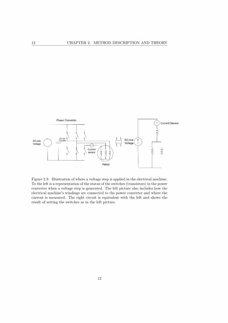
Figure 3.2: Equivalent circuit model of the electrical machine under test. Not seenin this picture is the mutual inductive coupling factor between the phase windings.Also not seen in the picture are the series resistance of the winding inductances.

3.1.2 Description of the model

The electrical simulation model can be seen in figure 3.2. The model includes thethree phases of the electrical machine in star configuration. The power converter

15


is represented by a voltage source that is set to produce a voltage step with thesame properties as the voltage step in reality in terms of magnitude, rise timeand pulse width. Every phase winding is represented by two inductances in series.The main reason for this compared to only having every phase represented by oneinductance is that the parasitic capacitances in the model now can be connected inthe middle of the winding instead of at the beginning or in the end of a winding.This influences the behavior of the circuit. The inductances also have a seriesresistance. The values used for the inductances and series resistances are takenfrom measurements done with an impedance analyser. The measurements withthe impedance analyser are attached to this report and can be seen in (ApendixA).

The phase-to-ground parasitic capacitance is connected between the mid points ofeach winding to a common node in the model representing the chassis. The phase-to-phase parasitic capacitances are connected directly between the mid points ofthe phase windings, equivalent with a delta connection. Both the phase-to-groundand phase-to-phase capacitances used in the model have both been measured withan impedance analyser and calculated from the known geometry of the stator. Themeasurements with the impedance analyser are attached to this report and canbe seen in (Apendix A). The calculations of the capacitances can be seen earlierin this chapter under the section Parasitic capacitance calculation.

3.1.3 Mutual Inductance

The developed electrical model also accounts for the mutual inductance betweenthe phases of the electrical machine. The mutual inductance is represented by amagnetic coupling factor between all of the phases. The coupling factor betweenthe two inductances that belongs to the same phase is presumed to be high, k =0.99. The coupling factor between the first phase and the other two are set to-0.5. This comes from the assumption that all windings magnetomotive forceare ideally sinusoidally distributed. This makes the phase windings shifted 120electrical degrease from each other which corresponds to a coupling factor of k =Cos(120°) = −0.5. The coupling factor between the two last phases in the modelis k = cos(−120°) = cos(240°) = −0.5.

16

3.2. SIMULATED CURRENT RESPONSE 17

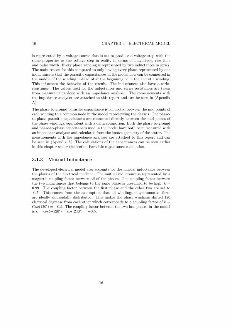
Figure 3.3: Current response from the simulation model without any simulatedfault. The green curve is the current and the blue one is the voltage.

3.2 Simulated current response

The final developed circuit is seen in 3.2. A simulated current response from a50 volt voltage step is seen in figure 3.3. The step is chosen to be 50 volts in thesimulation model and in the measurements. The same voltage level for all carriedout test was kept at 50 volts to have consistency and to be able to compare resultsbetween measurements as easy as possible. The exact amount of 50 volt is chosenbecause the capacitors used for the simulated faults are rated to 50 volts. Thevoltage level is in no way limited to be this low and could just as easily have beenchosen to another value.

17


18

Chapter 4

Experimental Procedure

4.1 Implementation

The experiments conducted during this master thesis project were done in theM-building at Faculty of Engineering - Lund University (LTH) in Lund in theelaboration room named Lab 6. The tests have mainly been performed on aPMSM referred to as H5M1 Hägglunds BAE. If nothing else is mentioned thenthat means that this electric machine was used. Some additional tests has alsobeen carried on a similar, but not exactly alike, machine referred to as H5M2 IEALTH and some tests has been done on a different, larger PMSM referred to asRasmus’ machine. The purpose of these additional test has been mainly to try themethod on other machines and compare the results. The equipment used is foundin list-form under the header Equipment used 4.1.7.

4.1.1 Test Set-up

The test set-up consists of the PMSM itself, motor control as well as high frequencycurrent sensing and logging. A block diagram of the set-up is seen i figure 4.1.The PMSM is placed on an a large iron foundation which is grounded (ProtectiveEarth). The electric machine is star connected through a connection box to thepower converter which is located inside an electrical cabinet. The cables used areshielded except for a short distance of approximately one decimetre before andafter the connection box. The cable length between the PMSM and the powerconverter is proximately three meters. The cable is of the type ölflex classic 110cy 4 g 16 rohs, 1135624. The power converter that runs the PMSM is controlledwith a Compact Reconfigurable Input Output (cRIO). The current sensor usedis placed around one of the phase cables between the power converter and thePMSM. When measurements are conducted in another phase the current sensor ismoved to that particular phase cable. The current logging is done on a Red Pitaya

19

20 CHAPTER 4. EXPERIMENTAL PROCEDURE

which for the intents and purposes of this thesis basically is a fast AD-converter,a Field-Programmable Gate Array (FPGA) and a memory.

Figure 4.1: Block diagram of the test set-up.

4.1.2 Test object 1

As stated in the introduction to this section the main test object is called H5M1Hägglunds BAE. A picture of this machine can be seen in figure 4.2. It is asix pole, three phase PMSM with the power ratings 12 kW continuous and 22 kWpeak power. It has a maximum speed rated to 15000 revolutions per minute (rpm)and a peak torque of 100 Nm. Furthermore the stator contains 24 slots with twowindings per slot. Each winding consists of eight turns which in turn consists ofeight strands of copper. [6].

4.1.3 Test object 2

For some additional test a larger eight pole, 18 slots PMSM has been used. Apicture of this machine can be seen in 5.15. This machine is rated to 80 kWcontinuous and 180 kW peak power. It has a peak torque of 250 Nm and amaximum speed of 15000 rpm. The machine is a prototype build and designed byRasmus Andersson and is referred to as Rasmus’ machine. This machine has beenused to carry out tests to evaluate temperature dependency since this machineis equipped with five Pt-100 temperature sensors. It has also been used in thepurpose of trying out the method on a larger machine and a machine with sixinstead of eight poles.[3]

4.1.4 Motor Control

The PMSM is run by a 3-phase power converter controlled by a cRIO system. Aspecific program for control of the PMSM for the purpose of this fault detection

20

http://www.ni.com/compactrio/

4.1. IMPLEMENTATION 21

Figure 4.2: Picture of the PMSM under test.

method has been developed and programmed in Labview. Both the cRIO systemand the Labview software are products of National Instruments. The developedcontrol program is written so that voltage pulses of variable pulse width can begenerated corresponding to going from switch state (0,0,0,) to (1,0,0,), (0,1,0,)and (0,0,1,) respectively. The pulse width can be varied from one tenth of amicro second and up. The limit of this tenth of a micro second is a consequenceof how the program is written and the internal clock of the cRIO FPGA. Theprogram uses four ticks of the internal FPGA clock for one loop and one ticktakes 25 nano seconds. The dc-link voltage, that for these active switch statesalso becomes the voltages over the windings, can be manually regulated througha variable transformer. The dc-link voltage can be varied at least between 15 and400 volts.

4.1.5 Current measurement

The phase current is measured with the current probe A6303 and the current probeamplifier Tektronix AM 503 when the machine is subjected to a voltage step. Thiscurrent sensor is able to measure currents up to 60 MHz. The current sensor isconnected to a Red Pitaya which is a circuit board containing among other thingsan FPGA , a processor and Random Access Memory (RAM) . The Red Pitayaalso has fast Analogue to Digital Converters (ADCs) and their by fast analogueinputs. The Red Pitaya’s analogue inputs has a sample rate of 125 Mega Samplesper second (MS\s). It was also tried to measure the current response with a CWTRogowski current probe named CWT3B but it proved to have to low resolutionto accurately display the current response.

21

http://sweden.ni.com/labview

http://www.ni.com

http://redpitaya.com/


4.1.6 Data logging

The Red Pitaya which is programmed in MATLAB is programmed in such a waythat it triggers on a rising voltage slope on one channel and measure the highfrequency current on a second channel. The program is written so that whenthe data buffer is filled with data, which takes 131 micro seconds, the programis automatically directly ready to trigger on a new voltage pulse and take newmeasurements. This makes it very easy to quickly do, for instance, a series often measurements just by applying ten fast voltage pulses with the motor controlprogram written in Labview. For the purpose of verifying the function of theRed Pitaya measurements was done were data gathered by the Red Pitaya wascompared with the data obtained from an oscilloscope.

4.1.7 Equipment used

Most of the equipment used is described more thoroughly in other sections. Hereis the most relevant equipment used in list form.

• Red Pitaya

• Current probe A6303 and the current probe amplifier Tektronix AM 503

• cRIO system

• Cable of the type Ölflex classic 110 cy 4 g 16 rohs, 1135624.

4.1.8 Performed tests

A large number of tests are performed. All of the test results that are used comesfrom a mean value of ten different current responses from ten different measure-ments done with the same settings. Firstly the current response is measuredseparately in each of the three phases; U,V and W. Then, the current response isalso measured in all the three phases separately for four different rotor positions.These measurements only becomes 10 ∗ 3 ∗ 4 = 120 measurements. Measurementswith different dc-link voltage of 50 and 100 volts are also made. In order to simu-late a fault or a developing fault measurements are done with different capacitorsplaced in parallel with one phase. Measurements are then performed and analysedfor both the phase parallel with the fault and the other phases. To study theinfluence of the cables used measurements with the current probe placed as closeto the inverter as possible, instead of right before the electrical machine, are alsodone. Measurements with an electrical machine in higher temperature are alsodone to study if a warmer machine effects the results of the measurements.

22

http://redpitaya.com/

http://www.ni.com/compactrio/

4.2. DATA ANALYSIS 23

4.2 Data Analysis

The data analysis is done in MATLAB. A program is written that stores the datacollected by the Red Pitaya on a computer. The data is analysed in the time andfrequency domain. The MATLAB-program does some post processing of the dataand is able to produce a comparative fault indicator value that is based on thedifference in frequency content from healthy measurements and the recently takenmeasurements. The MATLAB program is also able to plot the current responsein the time and frequency domain. More details of what post processing the datagoes through is found in the chapter 5 Analysis and results .

23


24

Chapter 5

Analysis and results

5.1 Characteristics of the current response

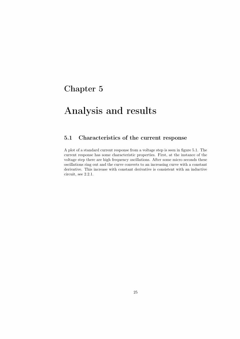
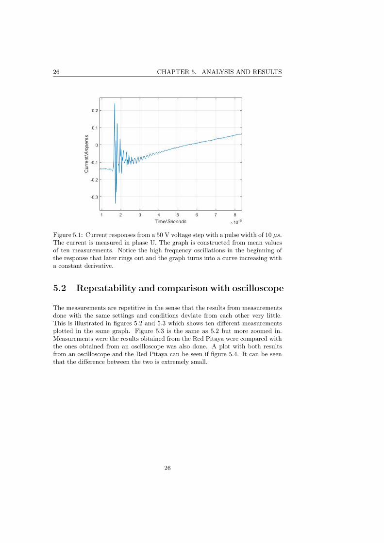
A plot of a standard current response from a voltage step is seen in figure 5.1. Thecurrent response has some characteristic properties. First, at the instance of thevoltage step there are high frequency oscillations. After some micro seconds theseoscillations ring out and the curve converts to an increasing curve with a constantderivative. This increase with constant derivative is consistent with an inductivecircuit, see 2.2.1.

25

26 CHAPTER 5. ANALYSIS AND RESULTS

Figure 5.1: Current responses from a 50 V voltage step with a pulse width of 10 µs.The current is measured in phase U. The graph is constructed from mean valuesof ten measurements. Notice the high frequency oscillations in the beginning ofthe response that later rings out and the graph turns into a curve increasing witha constant derivative.

5.2 Repeatability and comparison with oscilloscope

The measurements are repetitive in the sense that the results from measurementsdone with the same settings and conditions deviate from each other very little.This is illustrated in figures 5.2 and 5.3 which shows ten different measurementsplotted in the same graph. Figure 5.3 is the same as 5.2 but more zoomed in.Measurements were the results obtained from the Red Pitaya were compared withthe ones obtained from an oscilloscope was also done. A plot with both resultsfrom an oscilloscope and the Red Pitaya can be seen if figure 5.4. It can be seenthat the difference between the two is extremely small.

26

5.2. REPEATABILITY AND COMPARISON WITH OSCILLOSCOPE 27

Figure 5.2: Plot with 10 measurements of current responses from 50 V voltagesteps with a pulse width of 10 µs.

Figure 5.3: Plot with 10 measurements of Current responses from 50 V voltagesteps with a pulse width of 10 µs. Same as 5.2 but more zoomed in.

27


Figure 5.4: Plot with measurements from both the Red Pitaya and an oscilloscope.

28

5.3. ROTOR POSITION DEPENDENCY 29

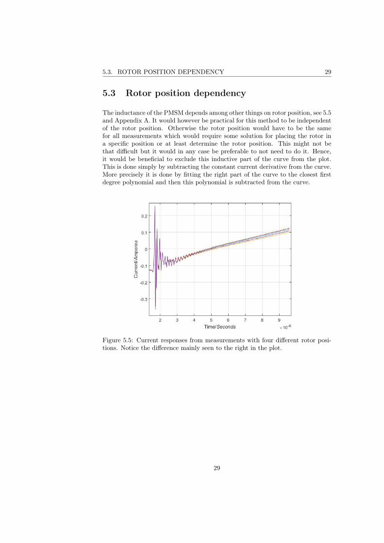
5.3 Rotor position dependency

The inductance of the PMSM depends among other things on rotor position, see 5.5and Appendix A. It would however be practical for this method to be independentof the rotor position. Otherwise the rotor position would have to be the samefor all measurements which would require some solution for placing the rotor ina specific position or at least determine the rotor position. This might not bethat difficult but it would in any case be preferable to not need to do it. Hence,it would be beneficial to exclude this inductive part of the curve from the plot.This is done simply by subtracting the constant current derivative from the curve.More precisely it is done by fitting the right part of the curve to the closest firstdegree polynomial and then this polynomial is subtracted from the curve.

Figure 5.5: Current responses from measurements with four different rotor posi-tions. Notice the difference mainly seen to the right in the plot.

29


Figure 5.6: Current responses from measurements with four different rotor po-sitions after the subtraction of the constant current derivative. Notice that theearlier difference between the for curves, seen in figure 5.5,now is difficult to observeat all.

5.4 Effects of changed parasitic capacitance

The current response can be studied either in the time or frequency domain. Boththese approaches are pursued. In figures 5.8 and 5.9 the effects of a simulatedfault of 1 nF parallel with one phase can be observed in the time and frequencydomain respectively. An illustration of where the fault capacitor is placed is seenin figure 5.7. In both plots, but perhaps most easily in 5.9, it can be seen that themain frequency is lower when a 1 nF capacitor is connected in parallel with onephase. This is expected since a capacitor in parallel corresponds to an increase incapacitance which leads to a decrease in resonance frequency. One way to noticea change of the parasitic capacitances could thus be to look at what frequency thehighest peak in the amplitude spectrum is through Fast Fourier Transform (FFT).Another way is look at the difference in amplitude spectrum at a certain frequencyband.

30

5.4. EFFECTS OF CHANGED PARASITIC CAPACITANCE 31

Figure 5.7: Illustration of where the fault capacitor, the simulated fault, is addedin the circuit. It is placed parallel to phase U.

Figure 5.8: Current responses from measurements with a simulated fault. Thevoltage step used is of 50 V. The blue curve is from the default set-up and the redcurve is from measurements done with a 1 nF capacitor in parallel with phase U.

31


5.5 Difference in frequency content

In figure 5.8 there is a clear difference in frequency content in the current responsewhen a fault of 1 nF is present. But what is a good way to identify a fault or adeveloping fault through use of the amplitude spectrum and how small faults canbe detected and distinguished from noise. This is investigated. In figure 5.10 thedifference between the FFT:s of current responses can be seen.

Figure 5.9: Amplitude spectrum of the current responses from a 50 V voltage stepof 10 us applied in phase U. The blue curve is from the default set-up without anyfault capacitor and the red curve is from measurements done with a 1 nF capacitorin parallel with one phase as showed in figure 5.7

5.6 Accuracy

An important and interesting factor for a method such as the one proposed in thisthesis is to know how small of a change that can be detected using the method.More precisely for this method this means to be able to say with certainty that theobserved change is from a change of the impedance of the PMSM and not fromany noise, disturbance or any other error source. In order to do this measure-ments with simulated faults of different capacitances are analysed and a way toproduce a numeric comparative fault indicating value is developed. A plot of thedifference in amplitude spectrum from measurements with different fault capaci-tors can be seen in figure 5.10. Figure 5.11 illustrates how much a measurementcan deviate from the original curve without necessarily being a sign of a developingfault. The figure shows the absolute value of the difference in amplitude spectrum

32

5.6. ACCURACY 33

from measurements with different fault capacitors. It also includes the differencein amplitude spectrum between different measurements of a healthy machine atdifferent rotor positions.

Figure 5.10: Difference in amplitude spectrum between measurements with a faultcapacitors added in parallel to one phase and measurements from a healthy ma-chine. Essentially the default amplitude spectrum with no fault capacitor sub-tracted with the amplitude spectrum of the current response with a fault capacitorconnected in parallel.

Figure 5.11: Absolute value of the difference in amplitude spectrum from measure-ments with different fault capacitors. Three graphs from similar measurementsfrom a healthy machine at different rotor positions are also included. The healthymachine measurements are the red curves.

33


Fault condition Fault Indicator Value100 pF 7.5433 pF 2.5915 pF 1.02Error threshold value 0.94

Table 5.1: Shows the single phase fault indicator value for some different simulatedfaults. The error threshold value, the value that the fault indicator value needs tobe higher than to statistically ensure that a change of impedance has occurred, isalso included.

5.7 Comparative fault indicator value

A way to produce a comparative numeric value which indicates the severity of adeveloping fault is suggested here. The proposed method is based on comparingthe difference in the amplitude spectrum of a recent series of measurements withcorresponding measurements from a healthy machine. The way to reach this faultindicator value goes as follows. First the amplitude spectrum where the mostfrequency content is present is chosen. For the studied machine in this project itwas chosen to be between 3.75 and 25 MHz. This can be seen for instance in figure5.10. Then the absolute value of the difference at every frequency (steps of 1250Hz) is summed up. This becomes 1700 values. This sum then becomes the FaultIndicator Value.

This fault indicator value can be constructed from measurements from the threedifferent phases. By doing so it is possible to see in what phase the developingfault is located or if it is a symmetrical fault. Values from measurements in thethree phases with a fault capacitor of 100 pF parallel with phase U, can be seenin 5.2.

5.7.1 Error threshold value

The meaning of, and the way the error threshold value is reached is covered here.In short it is a value that the fault indicator value needs to be higher than to sta-tistically ensure that a change of impedance has occurred. This value is reachedin the following way. Twelve series of measurements were every series of measure-ments consists of the mean value from ten measurements were taken. These twelveseries of measurement were from the three different phases with four different rotorpositions. Then the steps for generating the fault indicator value were taken forall the combinations of rotor positions for each phase. Meaning comparing rotorposition one through four in all six combinations possible for the three phases.This gives 18 values. The mean value, standard deviation and 95 percent confi-dence interval were then calculated. The mean value was 0.5633 and the standarddeviation was 0.1534. If normal distribution is presumed then the 95 percent con-fidence interval from these parameters with 18 measurements is +-0.07, meaningthat the mean value of the whole distribution, with a 95 percent probability, is

34

5.8. INFLUENCE OF CURRENT SENSOR LOCATION 35

Fault condition Measured phase Fault Indicator Value100 pF parallel phase U U 8.22100 pF parallel phase U V 2.06100 pF parallel phase U W 2.24

Table 5.2: Shows the Fault Indicator Value from measurements from the threedifferent phases from a simulated fault of 100 pF parallel to phase U.

within the interval 0.5633+-0.07. Then if normal distribution again is presumedthe fault indicator value has to be over 0.5633 + 0.07 + 2*0.1534 = 0.9401 to witha 95 percent certainty guarantee that a change of impedance has occurred. Thisvalue is called the error threshold value. The factor two in the calculation comesfrom that two standard deviations corresponds to the 95.4 percent percentile innormal distribution.

5.8 Influence of current sensor location

To study if and how much the measurements would be affected if the current probewas placed closer to the power converter, measurements with the current probeplaced as close to the power converter as possible were done. This means thatthe current probe was placed at the same cable but roughly three meters closerto the converter. The results of the series of measurements done showed that thethe current response indeed was significantly different. The two different currentresponses can be seen in figure 5.12 and the amplitude spectrum of the signalscan be seen in figure 5.13. The biggest reason for this large difference in highfrequency current is probably the parasitic capacitance of the cable itself. Eventhough the capacitance between the different conductors and between the conduc-tors and ground is small it still has a rather great influence at the high frequencies(approximately 7 MHz) that are studied. An equivalent circuit representation ofa cable can be seen in figure 6.1. This makes the accuracy of the, in this thesis,suggested fault detection technique susceptible to moving of the current sensors orchanging of the cables between the power converter an the electric machine.

35


Figure 5.12: High frequency current response right before the electric machine(usual) and right after the power converter (cabinet). The word cabinet refers tothat the current probe was placed inside the cabinet containing the power converteretcetera. In the plot there are measurements from two series of measurements fromthe cabinet.

Figure 5.13: Amplitude spectrum of the current response right before the electricmachine (usual) and right after the power converter (cabinet).

5.9 Thermal dependency

To analyse the thermal dependency a series of measurements have been done witha PMSM placed inside an isolated cage. These test was not done on the PMSM

36

5.9. THERMAL DEPENDENCY 37

Sensor number Sensor name Description1 Uhotspot Located at the expected hot spot, halfway

along the machine in the middle of a slot inone of the phases (phase U)

2 Ustatorback Located at the stator back outside the slotcontaining sensor 1

3 NDE Located at the bearing on the non-driving end4 DE Located at the bearing on the driving end5 Uendwinding Located on the end windings from the slot con-

taining sensor 1 (phase U)

Table 5.3: The temperature sensors of the PMSM under thermal test.

most used in this project but on another, larger PMSM, referred to as Rasmus’machine. Measurements have first been done in room temperature, about 23degrees and then with the machine at a temperature of approximately 50 degrees.The machine was heated externally with a heating gun. The measurements weredone when the temperature sensors had stabilised after the heating process. Theelectrical machine used for these measurements has five PT100 RTD temperaturesensors. A table of where these are placed is seen in table 5.3 and a picture of theplacement is seen in figure 5.14. A table of the status of the sensors before andafter heating is shown in table 5.4. Pictures of the machine under test and thethermal cadge used is shown in figures 5.15 and 5.16.

Figure 5.14: Temperature sensor positions in the PMSM used for thermal tests.

It might be difficult to see from the amplitude spectrum in figure 5.17 but it iseasily seen in the zoomed-in version in figure 5.18 that there is a small change infrequency content when the machine is 50 degrees Celsius compared to when itis 23 degrees. The earlier described fault indicator value for the heated machinefrom these measurements becomes approximately 1.5 which means that it is higherthan the error threshold value of 0.94 and thereby it is statistically certified at a 95percent confidence rate that a change of impedance has occurred. However eventhough there is a change, the change is very small.

37


Sensor Sensor name Rbefore Rafter Tbefore Tafter1 Uhotspot 109,281 119,303 23°C 48°C2 Ustatorback 109,222 119,293 23°C 48°C3 NDE 109,279 119,246 23°C 48°C4 DE 109,269 119,612 24°C 49°C5 Uendwinding not available (n\a) n\a n\a n\a

Table 5.4: Status of the temperature sensors during test.Rbefore is the resistanceof the PT100 resistors before heating, at the temperature of the reference mea-surements. Rafter is the resistance after heating, at the temperature of the mea-surements done in higher temperature. Tbefore and Tafter are the temperaturescorresponding to the resistance of the PT100 sensors.

Figure 5.15: The PMSM placed inside an isolated cage for the purpose of inves-tigating thermal dependency.

Figure 5.16: The isolated cage containing the PMSM.

38

5.9. THERMAL DEPENDENCY 39

Figure 5.17: Amplitude spectrum from measurements in room temperature andat approximately 50 degrees Celsius.

Figure 5.18: Amplitude spectrum from measurements in room temperature andat approximately 50 degrees Celsius, zoomed in.

5.9.1 Larger machine

The results from the tests done on Rasmus’ machine can also be compared withthe test done on the smaller machine. Compare for instance figures 5.17 with 5.9.It can be seen that the amplitude spectrum of the larger Rasmus’ machine containslower frequencies compared to the usual machine. The largest frequency contentin the smaller machine’s amplitude spectrum is found around the frequency 6.7MHz compared to 4.5 MHz for Rasmus’ machine. This means that the currentsensor and the data logging equipment needed can be slightly slower for Rasmus’machine.

39


40

Chapter 6

Comparison of model andmeasurements

If the measurements done are compared to the results given from the simulationmodel some difference can be noted. If the comparison is done between figures 5.1and 3.3 which are current responses from a 50 volt voltage step from measurementscontra the simulation, the behavior, amplitude and frequency of the oscillationsare quite similar to the results obtained from the measurements. However, onedirectly notices that the simulation gives a much cleaner and more regular cur-rent response compared to the measured one. The simulated signal has a cleardominating frequency which basically make up the whole signal compared to themeasured signal that consists of more spread frequencies. In figure 5.12 a plotfrom measurements where the current probe were placed right after the powerconverter, before the cable, can be seen. One notice that the current responsefrom this measurement is more similar to the plot obtained from the simulation(figure 3.3). This could be because the simulation does not account for the cable.Right after the power converter the current looks more like the simulation butafter the cable the high frequency current transient looks a bit different. At thehigh frequency, that the current transient has, the parasitic elements of the cableseems to have quite a large effect. Therefore a simulation model with a model ofthe cable also included was constructed.

Figure 6.1: Circuit representation of a cable.

41

42 CHAPTER 6. COMPARISON OF MODEL AND MEASUREMENTS

Figure 6.2: Equivalent circuit model of the electrical machine under test with amodel of the cables connecting the PMSM to the power converter also included.The current is measured right before phase U, after the cable.

Figure 6.3: Current response from the simulation model with a cable model addedas in figure 6.1. The red curve is the current and the green one is the voltage.

It is noticeable that the new simulated current response is more similar to themeasured values obtained in the sense that the frequency content is more spread.The behavior in terms of frequency and amplitude is in the same range as themeasurements. However the similarities stops there. To simulate a current re-sponse that in detail looks like the measured current response a better model isneeded.

42

Chapter 7

Conclusion and future work

7.1 Conclusion

This method for detecting developing faults in the stator insulation looks promis-ing. It is shown that small changes of insulation (corresponding to a 15 pF ca-pacitor parallel with a phase) can be detected with the method and equipmentused in this thesis project. This small of an impedance change is estimated tooccur long before a stator insulation fault is present. In this sense the methodworks satisfactory. There is no reason for this method not to work that has beenfound during this master thesis project. There are however some aspects that theimplementer of this method needs to be aware of. These are listed below.

• First of all the method does not detect all kinds of faults but only faultsrelating to the stator insulation. It does not detect rotor or bearing relatedfaults. However a method that detects 37 % of all failures, which is theapproximate number of how many failures that are related to stator windingproblems according to [10][p131], before they occur, is still highly interesting.

• It is difficult to, with precision, relate how much the current response canchange before a fault occurs. To do this one would need data from othersimilar machines that has been run until breakdown. One can however makea less exact estimation based on simulated faults.

• The proposed method is highly sensible to movement of the current sensor toanother place on a cable or changing anything that influences the impedancestructure of the circuit consisting of the power converter, the electrical ma-chine and the cables between them. Knowing this one could however workaround this issue.

• The method requires that current of a high frequency can be measured and

43

44 CHAPTER 7. CONCLUSION AND FUTURE WORK

logged.

7.1.1 Hardware requirements

One of this thesis project purposes was to look into what the minimumhardware requirements would be to implement this method in a vehicle.This basically comes down to one thing. The current needs to be measuredand logged at a high frequency which require a fast current sensor as wellas a fast ADC. Other than this the equipment needed for implementation isbasically already present in a hybrid or electric vehicle today. Exactly howhigh of a frequency that needs to be measured varies between machines. Forthe machine most tested in this thesis project, currents at at least five MHzneeds to be able to be measured. This is illustrated for example in figure 5.11where it can be seen that the frequency content difference between a healthymachine and one with a simulated fault is significantly smaller below circa5 MHz. This means that the sampling needs to be significantly faster thanthis and thereby the current sensor and the ADC needs to be significantlyfaster than 5 MHz.

7.2 Suggestions for Future work

7.2.1 More extensive testing

To fully evaluate this method a good approach would be to do the measurementson some healthy, identical, electrical machines and then subject the machines toenhanced ageing while taking measurements along the way. This would have tobe done until machine breakdown occurs for the machines. This would generatea library of data that could be compared with other machines. Then hopefullyit could be determined with high precision and likelihood how long a particularmachine is from insulation break down.

7.2.2 Better electrical model

With more knowledge and time it would be possible to improve the electricalmodel. With a more sophisticated model it might be possible to , amongst otherthings, analyse certain small changes in the current response and be able to seewhich type of impedance change in the electrical machine a particular change ofthe current response corresponds to.

44

References

[1] Fadi Abdallah. “EMC Analysis of Electric Drives”. Licentiate Thesis. LundUniversity, 2012.

[2] Kenneth W. Alley Charles L.; Atwood. Electronic Engineering, 3rd Ed. NewYork John Wiley & Sons., 1973. isbn: 0-471-02450-3.

[3] Rasmus Andersson. “Electric Traction Machine Design for Heavy HybridVehicles”. Licentiate Thesis. Lund University, 2014.

[4] S. Grubic, J. Restrepo, J. M. Aller, Bin Lu, and T. G. Habetler. “A NewConcept for Online Surge Testing for the Detection of Winding InsulationDeterioration in Low-Voltage Induction Machines”. In: IEEE Transactionson Industry Applications 47.5 (Sept. 2011), pp. 2051–2058. issn: 0093-9994.doi: 10.1109/TIA.2011.2161972.

[5] G. M. Joksimovic and J. Penman. “The detection of inter-turn short circuitsin the stator windings of operating motors”. In: IEEE Transactions on In-dustrial Electronics 47.5 (Oct. 2000), pp. 1078–1084. issn: 0278-0046. doi:10.1109/41.873216.

[6] F. J. Márquez-Fernández, Z. Huang, and M. Alaküla. “Redesign of an Electri-cal Rear Wheel Drive (E-RWD) for a hybrid vehicle in a given drive cycle”.In: Electrical Machines (ICEM), 2012 XXth International Conference on.Sept. 2012, pp. 2702–2708. doi: 10.1109/ICElMach.2012.6350268.

[7] P. Nussbaumer, T.M. Wolbank, and M.A. Vogelsberger. “Separation of dis-turbing influences on induction machine’s high-frequency behavior to en-sure accurate insulation condition monitoring”. In: Applied Power Electron-ics Conference and Exposition (APEC), 2013 Twenty-Eighth Annual IEEE.Mar. 2013, pp. 1158–1163. doi: 10.1109/APEC.2013.6520445.

[8] José Rodríguez. Senior Member. IEEE. Luis Morán. Senior Member. IEEE. JorgePontt. Member. IEEE. Ruben Osorio and Samir Kouro. “Modeling andanalysis of common-mode voltages generated in medium voltage PWM-CSI drives”. In: Power Electronics, IEEE Transactions on 18.3 (May 2003),pp. 873–879. issn: 0885-8993. doi: 10.1109/TPEL.2003.810855.

45

http://dx.doi.org/10.1109/TIA.2011.2161972

http://dx.doi.org/10.1109/41.873216

http://dx.doi.org/10.1109/ICElMach.2012.6350268

http://dx.doi.org/10.1109/APEC.2013.6520445

http://dx.doi.org/10.1109/TPEL.2003.810855

46 REFERENCES

[9] F. Perisse, P. Werynski, and D. Roger. “A New Method for AC Machine TurnInsulation Diagnostic Based on High Frequency Resonances”. In: Dielectricsand Electrical Insulation, IEEE Transactions on 14.5 (Oct. 2007), pp. 1308–1315. issn: 1070-9878. doi: 10.1109/TDEI.2007.4339494.

[10] G. C. Stone, E. A. Boulter, I. Culbert, and H. Dhirani. Electrical insula-tion for rotating machines-design, evaluation, aging, testing, and repair. theInstitute of Electrical and Electronics Engineer Inc., 2004.

[11] G. C. Stone, E. A. Boulter, I. Culbert, and H. Dhirani. Electrical insula-tion for rotating machines-design, evaluation, aging, testing, and repair. theInstitute of Electrical and Electronics Engineer Inc., 2004, p. 131.

[12] S. J. Williamson, R. Wrobel, J. D. Booker, J. Yon, and P. H. Mellor. “Effectsof Insulation Ageing on the Conductive Heat Transfer from the WindingBody into Machine Periphery/Stator Core Pack”. In: - - (2016).

[13] J. Yang, J. Cho, S. B. Lee, J. Y. Yoo, and H. D. Kim. “An Advanced Sta-tor Winding Insulation Quality Assessment Technique for Inverter-Fed Ma-chines”. In: IEEE Transactions on Industry Applications 44.2 (Mar. 2008),pp. 555–564. issn: 0093-9994. doi: 10.1109/TIA.2008.916753.

[14] C. Zoeller, M.A. Vogelsberger, R. Fasching, W. Grubelnik, and T.M. Wol-bank. “Evaluation and current-response based identification of insulationdegradation for high utilized electrical machines in railway application”. In:Diagnostics for Electrical Machines, Power Electronics and Drives (SDEMPED),2015 IEEE 10th International Symposium on. Sept. 2015, pp. 266–272. doi:10.1109/DEMPED.2015.7303700.

46

http://dx.doi.org/10.1109/TDEI.2007.4339494

http://dx.doi.org/10.1109/TIA.2008.916753

http://dx.doi.org/10.1109/DEMPED.2015.7303700

Appendix

47

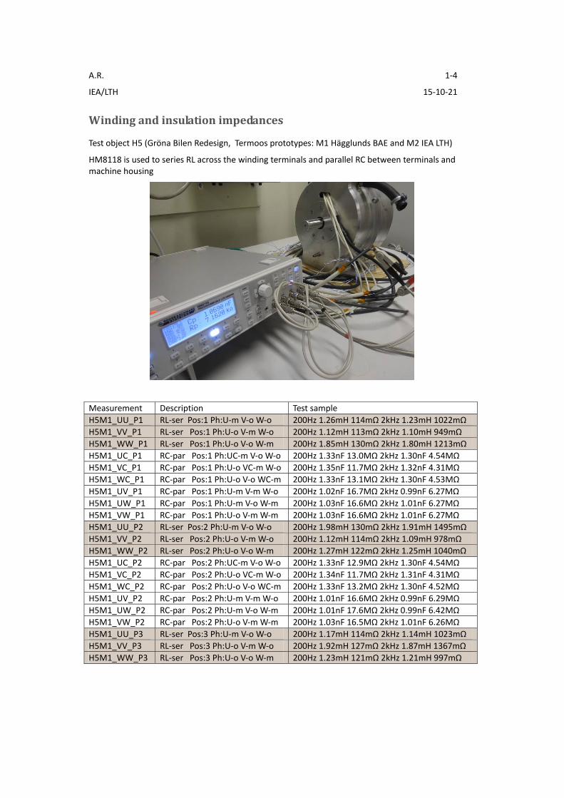
A.R. 1‐4

IEA/LTH 15‐10‐21

Winding and insulation impedances

Test object H5 (Gröna Bilen Redesign, Termoos prototypes: M1 Hägglunds BAE and M2 IEA LTH)

HM8118 is used to series RL across the winding terminals and parallel RC between terminals and machine housing

Measurement Description Test sample

H5M1_UU_P1 RL‐ser Pos:1 Ph:U‐m V‐o W‐o 200Hz 1.26mH 114mΩ 2kHz 1.23mH 1022mΩ

H5M1_VV_P1 RL‐ser Pos:1 Ph:U‐o V‐m W‐o 200Hz 1.12mH 113mΩ 2kHz 1.10mH 949mΩ

H5M1_WW_P1 RL‐ser Pos:1 Ph:U‐o V‐o W‐m 200Hz 1.85mH 130mΩ 2kHz 1.80mH 1213mΩ

H5M1_UC_P1 RC‐par Pos:1 Ph:UC‐m V‐o W‐o 200Hz 1.33nF 13.0MΩ 2kHz 1.30nF 4.54MΩ

H5M1_VC_P1 RC‐par Pos:1 Ph:U‐o VC‐m W‐o 200Hz 1.35nF 11.7MΩ 2kHz 1.32nF 4.31MΩ

H5M1_WC_P1 RC‐par Pos:1 Ph:U‐o V‐o WC‐m 200Hz 1.33nF 13.1MΩ 2kHz 1.30nF 4.53MΩ

H5M1_UV_P1 RC‐par Pos:1 Ph:U‐m V‐m W‐o 200Hz 1.02nF 16.7MΩ 2kHz 0.99nF 6.27MΩ

H5M1_UW_P1 RC‐par Pos:1 Ph:U‐m V‐o W‐m 200Hz 1.03nF 16.6MΩ 2kHz 1.01nF 6.27MΩ

H5M1_VW_P1 RC‐par Pos:1 Ph:U‐o V‐m W‐m 200Hz 1.03nF 16.6MΩ 2kHz 1.01nF 6.27MΩ













A.R. 2‐4

IEA/LTH 15‐10‐21

102

103

104

105

0.4

0.6

0.8

1

1.2

1.4

1.6

1.8

2x 10

-3in

duct

ance

, L

[H]

102

103

104

105

10-1

100

101

102

103

resi

stan

ce,

R [

Ohm

]

frequency, f [Hz]

H5M1UU

P1.txt

H5M1V

VP1.txt

H5M1W

WP1.txt

H5M1UU

P2.txt

H5M1V

VP2.txt

H5M1W

WP2.txt

H5M1UU

P3.txt

H5M1V

VP3.txt

H5M1W

WP3.txt

102

103

104

105

1.25

1.3

1.35

1.4

1.45

1.5

1.55x 10

-9

capa

cita

nce,

C [

F]

102

103

104

105

103

104

105

106

107

108

resi

stan

ce,

R [

Ohm

]

frequency, f [Hz]

H5M1UC

P1.txt

H5M1V

CP1.txt

H5M1W

CP1.txt

H5M1UC

P2.txt

H5M1V

CP2.txt

H5M1W

CP2.txt

102

103

104

105

0.98

1

1.02

1.04

1.06

1.08

1.1

1.12

1.14

1.16

1.18x 10

-9

capa

cita

nce,

C [

F]

102

103

104

105

103

104

105

106

107

108

resi

stan

ce,

R [

Ohm

]

frequency, f [Hz]

H5M1UV

P1.txt

H5M1V

WP1.txt

H5M1V

WP1.txt

H5M1UV

P2.txt

H5M1UW

P2.txt

H5M1V

WP2.txt

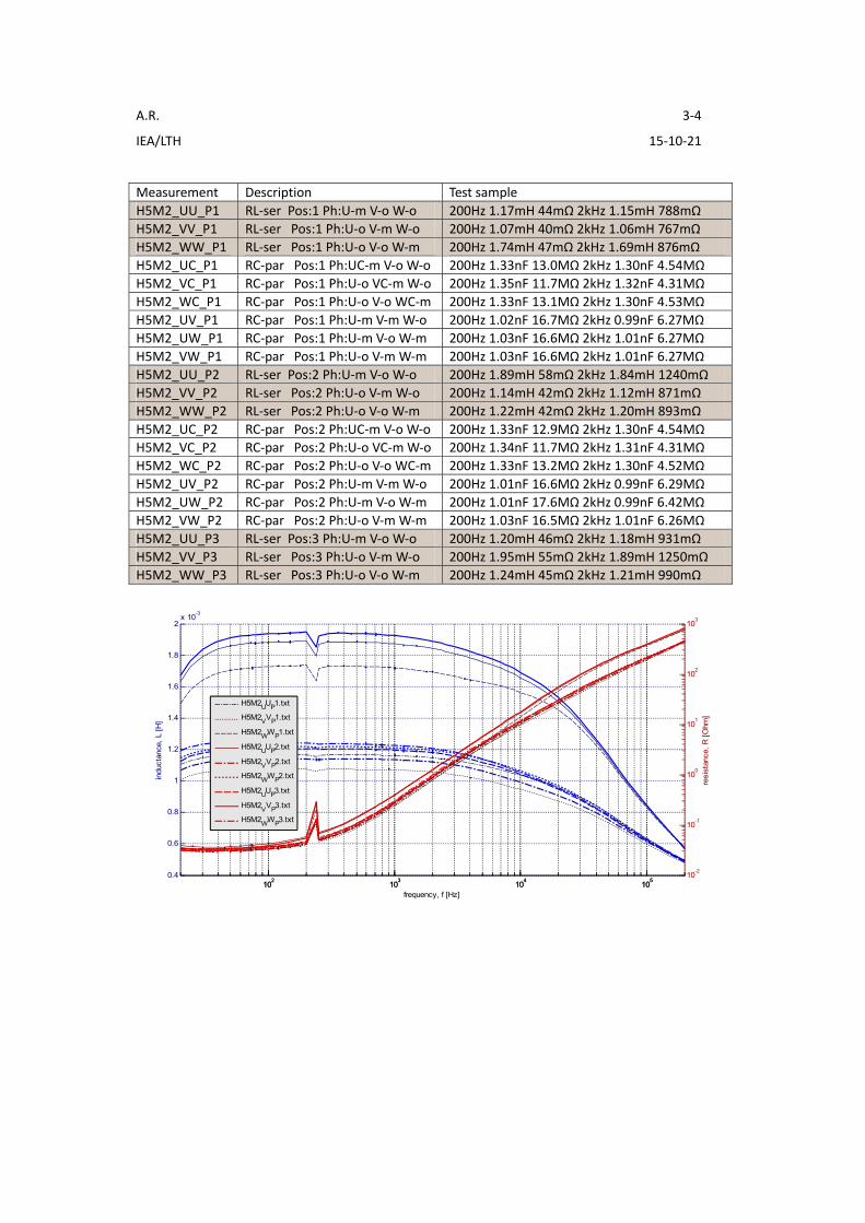
A.R. 3‐4

IEA/LTH 15‐10‐21

Measurement Description Test sample






















102

103

104

105

0.4

0.6

0.8

1

1.2

1.4

1.6

1.8

2x 10

-3

indu

ctan

ce,

L [H

]

102

103

104

105

10-2

10-1

100

101

102

103

resi

stan

ce,

R [

Ohm

]

frequency, f [Hz]

H5M2UU

P1.txt

H5M2V

VP1.txt

H5M2W

WP1.txt

H5M2UU

P2.txt

H5M2V

VP2.txt

H5M2W

WP2.txt

H5M2UU

P3.txt

H5M2V

VP3.txt

H5M2W

WP3.txt

A.R. 4‐4

IEA/LTH 15‐10‐21

102

103

104

105

6

6.5

7

7.5

8

8.5

9

9.5

10x 10

-10ca

paci

tanc

e, C

[F

]

102

103

104

105

103

104

105

106

107

108

109

resi

stan

ce,

R [

Ohm

]

frequency, f [Hz]

H5M2UV

P1.txt

H5M2V

WP1.txt

H5M2V

WP1.txt

H5M2UV

P2.txt

H5M2UW

P2.txt

H5M2V

WP2.txt

0-3-DIAGNOSTICSANDPROGNOSTICS - Lund … document/5373_full...0-3-DIAGNOSTICSANDPROGNOSTICS...

Documents

Transcript of 0-3-DIAGNOSTICSANDPROGNOSTICS - Lund … document/5373_full...0-3-DIAGNOSTICSANDPROGNOSTICS...