[Cathy hasn’t seen this version 54]

Predicting Future Years of Life, Health, and Functional Ability:

A Healthy Life Calculator for Older Adults

Paula Diehr, Depts of Biostatistics and Health Services, University of Washington, Seattle, WA. (pdiehr@uw.edu)

Michael Diehr, Dept of Psychology, California State University, San Marcos (mdiehr@csusm.edu)

Alice M. Arnold, Department of Biostatistics, University of Washington (arnolda@uw.edu)

Laura Yee, Department of Biostatistics, University of Washington (laurayee@uw.edu)

Michelle C Odden, College of Public Health and Human Sciences, Oregon State University (michelle.odden@oregonstate.edu)

Calvin H Hirsch, Departments of Internal Medicine and Public Health Sciences, UC Davis Medical Center, Sacramento, CA (chhirsch@ucdavis.edu)

Stephen Thielke, Department of Psychiatry, University of Washington; Geriatric Research, Education, and Clinical Center, Seattle VA Medical Center (sthielke@uw.edu)

Bruce M Psaty, Departments of Medicine, Epidemiology and Health Services, University of Washington; Group Health Research Institute of Group Health Cooperative, Seattle, WA (pasty@uw.edu)

W. Craig Johnson, Department of Biostatistics, University of Washington (wcraigj@uw.edu)

Jorge Kizer, Albert Einstein College of Medicine / Montefiore Medical Center (jorge.kizer@einstein.yu.edu)

Anne Newman, Graduate School of Public Health, University of Pittsburgh (anewman+@pitt.edu)

Corresponding Author Paula Diehr, pdiehr@uw.edu, box 34922, University of Washington, Seattle, WA, 98195

Key words: Prediction; aged; years of healthy life; activities of daily living; validation

Word count: Abstract 305; body of paper 5520. 4 tables. 8 appendices.

1

Predicting Future Years of Life, Health, and Ability:a Healthy Life Calculator for Older Adults

Abstract

Introduction

Planning for the future would be easier if we knew how long we will live and, more importantly, how many years we will be healthy and able to enjoy it. There are few well-documented aids for predicting our future health. We attempted to meet this need for persons 65 years of age and older.

Methods

Data came from the Cardiovascular Health Study, a large longitudinal study of older adults that began in 1990. Years of life (YOL) were defined by measuring time to death. Years of healthy life (YHL) were defined by an annual question about self-rated health, and years of able life (YABL) by questions about activities of daily living. Years of healthy and able life (YHABL) were the number of years the person was both Healthy and Able. We created prediction equations for YOL, YHL, YABL, and YHABL based on the demographic and health characteristics that best predicted outcomes. Internal and external validity were assessed. The resulting CHS Healthy Life Calculator (CHSHLC) was created and underwent three waves of beta testing.

Findings

A regression equation based on 11 variables accounted for about 40% of the variability for each outcome. Internal validity was excellent, and external validity was satisfactory. As an example, a very healthy 70-year-old woman might expect an additional 20 YOL, 16.8 YHL, 16.5 YABL, and 14.2 YHABL. The CHSHLC also provides the percent in the sample who differed by more than 5 years from the estimate, to remind the user of variability.

Discussion

The CHSHLC is currently the only available calculator for YHL, YABL, and YHABL. It may have limitations if today’s users have better prospects for health than persons in 1990. But the external validity results were encouraging. The remaining variability is substantial, but this is one of the few calculators that describes the accuracy of the estimates. Dissemination of this information requires a different approach than simply publishing the paper and presenting results at meetings.

Conclusion

2

The CHSHLC, currently at https://healthylifecalculator.org, meets the need for a straightforward and well-documented estimate of future years of healthy and able life that older adults can use in planning for the future.

Note: This paper has been published here:

http://journals.sagepub.com/doi/pdf/10.1177/2333721415605989

Most of the text in the body of this report is the same as the published paper. Section 4.4 about dissemination is new, as is section 4.5 about extrapolation to ages less than 65. The ten technical appendices contain new material, which may be of interest. The table of contents for the appendices is shown on about page 24. Appendices 1-6 were referred to in the published paper. The remainder are all new work, including the consideration of Cognition as an additional outcome (appendix 8). The appendices also address the inclusion of some “obvious” variables that did not satisfy the initial screening criteria, such as socio-economic status, obesity, and others (appendix 9); an estimate of the number of users of the web application (appendix 10); and comparison of several methods for generalizing the estimates to persons under age 65 (appendix 11).

3

1.0 Introduction

Older adults often need to make decisions about the future, including possible relocation from their current home. Those who expect a long and healthy life may plan for an active retirement and consider moving to a resort community. Those with worse prospects may choose instead to move near their children or to a retirement community with assisted care. It would help to have an estimate of how many healthy and active years older adults could anticipate, but there are no documented tools for doing so.

United States life tables (such as from the Social Security Administration 1 ) show the expected number of additional years of life, based on a person’s age and sex, but they do not incorporate health characteristics. There are no well-documented tools for estimating a person’s future years of healthy life, or years in which they will be able to perform basic activities of daily living (ADL).

Our goal was to develop useful and accessible estimates of total years of life, years of healthy life and years of life free of ADL difficulty, based on data from the Cardiovascular Health Study (CHS), a large longitudinal study of persons aged 65-99 at baseline. This manuscript describes the process of creating and evaluating the CHS Healthy Life Calculator (CHSHLC). Additional detail is available in the detailed methods appendices, described below.

2.0 Methods

2.1 Data

Description of CHS

The Cardiovascular Health Study (CHS), funded by the National Heart and Lung Blood Institute, recruited 5201 older adults in 1990 from Medicare eligibility lists in four U.S. communities. Persons who used wheelchairs at home, were under treatment for cancer, or were not expected to participate for 3 years after baseline were ineligible. More details about the study design can be found elsewhere. 2 CHS followed enrollees’ health from baseline in 1990 to the analysis date (2013), providing 23 years of follow-up. A second cohort of 687 African Americans began in 1993 and now has 20 years of follow-up. Participants were contacted every six months and were seen in the field centers annually through 1999, and again in 2005-06. Hundreds of health-related variables were collected at baseline and at the annual clinic visits and a fewer number were collected annually or semi-annually by phone throughout follow-up.

Dependent Variables

Two health-related variables were measured every year after baseline. Self-rated health was a single question, “is your health excellent, very good, good, fair, or poor?”, and “Healthy”

4

was defined as being in excellent, very good, or good health (as opposed to fair or poor health). Activities of daily living were defined as self-reported difficulty in walking around the house, getting out of a bed or chair, feeding, dressing or bathing oneself, and getting to and using the toilet. A person who had no difficulties with any of those activities was defined as “Able”. We summed the number of years when a person was Alive (YOL), Healthy (YHL), Able (YABL), and both Healthy and Able (YHABL). 3 These variables have been used as outcomes in other publications. 4 5 6 7 8 9 10

For the 85% of enrollees who died before 2013, the observed data were complete. We estimated the additional years for the remaining 15%. For example, for a person who was 65 at baseline and still alive 20 years later, the number of remaining years was estimated from persons who were age 85 and of the same sex, Healthy and Able status at baseline. (See Appendix 1). These estimates were added to the sum of the observed data to provide lifetime data for everyone. The lifetime sums were the outcome variables for the analyses.

Potential Predictor Variables

CHS collected hundreds of variables at the baseline intake. We sought to identify predictors that were associated with the outcomes, and to limit the total number so that they could be asked in a short questionnaire designed for lay persons. Here, we limited potential predictors to about 200 variables that had almost no missing values at baseline and that could be self-reported by the user. These requirements excluded laboratory test results, clinic measurements and lengthy questionnaires, as well as variables asked of only one sex. The variables also needed to be available at the baseline of each of the 4 waves. Space limitations do not permit listing all of the variables initially considered, but they included measures of personal history, medical history, physical function, cognitive function, physical activity, social support, quality of life, and stressful life events. (See Appendix 7).

Waves of Data

Missing values of self-reported health and activities of daily living during follow-up were imputed by linear interpolation of a person’s observed values over time. In brief, available data were transformed to a scale that included a value for death. Missing values were linearly interpolated over time for each person, and the resulting variables were transformed back to the original scale. Details are available elsewhere. 11 About 14% of the possible self-rated health data (when person was alive) had to be imputed, and about 29% of the ADL data. The latter number was large because ADL was not collected in the appropriate format from 2000 to 2004.

For this analysis, we created four waves of data, where wave 0 consisted of the baseline year and 20 years of follow-up for both cohorts. Wave 1, for the first cohort only, started 1 year after baseline and had 20 years of follow-up from year 1 to 21, and similarly for Waves 2 and 3

5

which started 2 and 3 years after the first cohort’s baseline, respectively and included 20 years of follow-up. There were thus 5201*4 + 687 = 21,491 potential baseline observations, and because some enrollees died in the first 3 years, there were actually 20,876 baseline observations. This approach allowed us to use all of the data, while maintaining the same number of years of follow-up for both cohorts, increased the number of the oldest persons available for analysis, and potentially reduced the likelihood of “healthy volunteer bias” because only about a fourth of the waves started at the true baseline. The disadvantage is that observations were not statistically independent (most persons were in the dataset four times). As described below, that was handled by restricting analyses where independence was required to a single wave of data.

2.2 Analysis

Selection of Predictor Variables

The goal was to predict YOL, YHL, YABL, and YHABL for a person with certain attributes. The prediction equations, separate for men and women, needed to include age and the baseline values of Healthy and Able. We next screened the potential baseline variables to identify a small set of variables that improved prediction. The variables were screened in two stages. The first stage screened the 200 or so potential variables, as described below and listed in Appendix Table 7.1. The second stage re-screened a subset of variables that users might expect to be included (see below), to improve the face validity of the eventual calculator. Stepwise multiple regressions were used for screening.

Screening for good predictors

The first screening forced baseline age, Healthy and Able into the regression, and then performed a forward selection regression among all of the remaining eligible baseline variables, with an alpha to enter of 0.0001. This screening used only Wave 0 data, so that observations were statistically independent and the significance levels had some meaning. Variables that were selected in all 8 of the regressions (4 outcomes for two sexes) were retained. The likelihood of false discovery was limited by the small alpha level and the requirement that the predictor be selected for both men and women.

Screening to improve face validity

The second screening forced in the regression variables chosen above, and then performed a forward selection among variables commonly associated with mortality, self-reported health or functional status in CHS, even though they were not selected in the first screen. A less stringent alpha level of 0.01 was used. The following variables were considered in the second screen: bed days in past two weeks, blocks walked in the previous week, hospitalization in the previous year, myocardial infarction, stroke, feeling about life as a whole, # of difficulties with instrumental activities of daily living (IADL), previous angioplasty, coronary bypass surgery, current diagnosis of cancer, taking insulin or hypoglycemic agents, renal disease

6

or failure, and body mass index. Variables were retained if they were selected in all or most of the 8 regressions. This screen was restricted to the Wave 3 data (which began 3 years after baseline) to ensure statistical independence and to reduce the healthy cohort bias. The variables selected at this stage were included in the main prediction equation.

In order to estimate years of healthy and able life, the final prediction equations used all of the selected variables, and were calculated using all waves of the dataset, because statistical significance was no longer an issue and the larger sample was important for estimation at the oldest ages.

2.3 Internal and External Validation

Internal validation involved random assignment of 80% of the enrollees into a “training” sample and the remaining 20% into a “validation ” sample. The 2-stage variable screening was repeated in the training sample only, and the resulting prediction equations were applied to the validation sample. The root mean squared error, defined as the square root of the average squared difference between observed and predicted values, was calculated. We also calculated the % of estimates that were within plus or minus 5 (or 3) years of the observed values. This process addressed the issues of over-fitting because the validation sample was not used in creating the prediction equations. Note that this type of validation does not test the specific variables chosen or the regression coefficients, but rather whether the methods used to create the estimates provided good estimates for the validation sample.

The external validation used two outside sources of data: the current U.S. lifetable [1] and unpublished data from a different cohort study. The life expectancies from the current U.S. lifetable are estimates of YOL. We compared the lifetable to the CHS estimates of YOL, and also to the observed data. There are no national estimates of YHL, and we found no study that was strictly comparable to CHS, which had nearly lifetime follow-up on self-rated health and activities of daily living. Instead, we used unpublished data from the Multi-Ethnic Study of Atherosclerosis (MESA), also funded by the NHLBI. 12 MESA enrollees, required to be free of heart disease at baseline, have been followed for 10 years to date. Self-rated health was collected at each survey wave. Using the approach outlined above, we calculated 10-year prediction equations for YOL and YHL in CHS, limiting to variables that were available in both CHS and MESA, plus a variable indicating heart disease that was set to 0 for all MESA enrollees (see findings section). We applied the new CHS equations to the MESA enrollees aged 65 and older, and compared the mean observed and predicted values.

2.4 Creation, Documentation and Beta Testing of the CHS Healthy Life Calculator (CHSHLC)

We created a web-based calculator (the CHSHLC) that requested the user to provide the information for the prediction equations, and then calculated the user’s lifetime expected values. The web page includes documentation in a frequently asked question (FAQ) format. Three

7

convenience samples of older adults were invited to use the calculator and provide feedback. After each wave we modified the calculator to reflect the user comments. See Appendix 2 for more detail.

3.0 Findings

3.1 Predictor Variables Chosen for the CHSHLC

Histograms of the four outcome variables are given in Appendix 1. Descriptive statistics are shown in the first four lines of Table 1, and are discussed below.

The eligible variables were entered into the regression several stages, as previously described. Analyses were done separately for men and women. In the first stage, baseline age was included both as a linear and a log term, to allow the relationship to be nonlinear where it was warranted. For baseline self-reported health, we included both the binary “Healthy” variable (1 if excellent, very good, or good; 0 if fair or poor) and also a recode of excellent through poor to 95, 90, 80, 30, and 15 respectively. 13 Baseline Able was coded as 0 if the person had difficulty with any of the ADLs, and 1 otherwise. (CHS had relatively few enrollees with 2 or more ADL difficulties). Baseline HABLE was coded as 1 if the person was both Healthy and Able, 0 otherwise.

The first screen of about 200 baseline variables selected four predictors: smoking, shortness of breath, diabetes, and number of prescription drugs. Smoking was coded as never, former, or current smoker. After the beta test we added the number of years since quitting for former smokers. Shortness of breath was based on self-report of the symptom when hurrying on the level or walking up a slight hill. It was significantly correlated with longer indices measuring COPD, CHF, and lack of fitness (not shown) and may be in part a proxy for those conditions. Diabetes was coded 1 for persons whose doctor had told them they had diabetes and 0 otherwise. Although fasting glucose was also measured at baseline, we used only the self-reported data because the calculator would also be based on self-report. The number of prescription drugs was not actually self-reported in CHS. Rather, enrollees brought their prescription drugs to the initial and annual interviews, where they were counted and classified. The variable was such a strong predictor, however, that we created a self-report question for the CHSHLC.

The second screen, meant to improve face validity chose 4 more variables: a history of MI or stroke, blocks walked in the last week, instrumental activities of daily living (IADL), and feeling about life as a whole. MI and Stroke were combined to a single question in the calculator. Number of blocks walked in the last week is a simple measure of physical activity. We changed the wording somewhat from the original questionnaire because nowadays many people know how many miles they walk, and the beta testers suggested this change. The variable was significantly related to the over-all physical activity scale (not shown) which was too lengthy to collect for this application. Instrumental activities of daily living (IADLs) were defined as any difficulty with housework, shopping, meal preparation, money management, or

8

using the telephone. The number of reported IADL difficulties, used on the log scale, was significantly correlated with the Modified Mini-Mental State Exam (not shown), which was available but too lengthy to collect for this application. Feeling about life as a whole (rated from delighted (1) to terrible (6)) was not as strong a predictor as the others (was not selected for all 8 regressions). But it has the added benefit of being significantly related to the CESD depression scale (not shown), which was too long for this application.

The descriptive statistics for the variables selected for the calculator and the 4 outcome variables are in Table 1. The first two columns are for Wave 0 (true baseline) only, and columns 3 and 4 show waves 0-3 combined. YOL through YHABL are the dependent variables; for example, in the complete data set, women averaged 13.43 YOL but only 6.87 YHABL. The averages for men were a little lower. Mean age at baseline was 73.8 for women and 74.6 for men. Only 48 enrollees were age 90 or older at the true baseline, but the extra waves of data provided a total of 245 persons over 90 for analysis (data not shown).

[Table 1 about here]

3.2 Predictions

The proportion of variability explained, R2, was .37 for YOL, and .41, .40, and .41 for YHL, YABL, and YHABL respectively. In the sex-specific regressions, age alone accounted for about 17% of the variability, baseline Healthy and Able for another 13%, the Screen 1 variables for 5 or 6%, and the Screen 2 variables account for another 2 or 3%. Additional information about R2 is shown in Appendix Table 3.

The 8 regression equations are shown in Table 2. “Coeff” is the regression coefficient and p is the significance level in the final equation. The coefficients should not be over-interpreted because the variables were chosen by screening for the most significant predictors rather than based on theory. The coefficient for age is not easily interpretable because ln(age) is also in the equation. Similarly, Healthy (binary) and self-rated health are both included, as are Able and “Healthy and Able”. None of those coefficients is directly interpretable because of multicollinearity. Three of the remaining variables were used on the log scale (ln(IADL+1) , ln(blocks walked + 1), and ln(# of medications+1)), also making their coefficients difficult to interpret directly.

The remaining coefficients are more directly interpretable. For example, for women, shortness of breath was associated with .6 fewer YOL, 1.2 fewer YHL, 1.0 fewer YABL, and 1.3 fewer YHABL, after controlling for the other variables in the equation. For women, diabetes was associated with 1.9 fewer YHL, current smoking with 3.1 fewer YHL, and so on. Variables were highly statistically significant except in the few cases that can be attributed to

9

multicollinearity. The significance levels are not surprising because of the way the variables were chosen.

[Table 2 about here]

Example of Predictions at Age 70

Table 3 provides an example of the predictions for 70-year-old women and men at several percentiles of health. For example, in row 1, for 70-year-old CHS women, mean observed YOL was 16.04 years, comparing favorably to a mean predicted value of 15.82 years. Unlike the lifetable estimate (16.33 years for all 70-year-old-women), we obtained a range of estimates based on personal characteristics. The fifth percentile of the predicted values was 10.80 years, the median was 16.32 years, and the 95th percentile was 18.98 years. For 70-year-old men the estimates of YOL were lower than for women, and the mean was slightly less than the lifetable estimate.

There is no national standard for YHL, YABL, or YHABL. The tabled results show that the mean observed and predicted values are close to each other, and that there is a large range of predicted values for both men and women. The CHSHLC estimates are thus close to the national standard (for YOL) and to the observed data, and produce a wide range of estimates rather than estimating everyone at the mean.

[Table 3 about here]

3.3 Internal and External Validity

Internal validity

To assess internal validity we repeated the process for creating the prediction rules in the training sample and applied the resulting rules to the validation sample. The same four variables were selected in the first screen of the training sample as in the over-all analysis. Although a few variables were different in the second screen, that is to be expected because those were not the most consistent predictors. The root mean squared error (RMSE), defined as the square root of the mean squared difference between the observed and expected values, was nearly identical in the training and validation samples. For example, RMSE for YOL was 5.96 years in the training sample and 6.05 years in the validation sample. The prediction was thus nearly as good in the validation sample as in the training sample. (See Appendix 4 for the complete RMSE data).

Because few of the potential users of the calculator will have any intuition for RMSE, we instead present Table 4, which shows the % of estimates that were within plus or minus 5 (or 3) years of the observed data. First consider YOL. Only 42% of the predicted values for 65-69-

10

year-olds were within + 5 years of the observed values, but the results improved with age. Prediction was better for YHL, YAL, and YHABL than for YOL. Similar results are given in the lower part of the table which shows the percent of estimates within 3 years of the observed values. Related tables for the % more than 5 years away from the observed are in Appendix 5. The percent above and below the 5-year interval were roughly comparable, and so can be approximated from Table 4 as (100-% within 5 years)/2. Personalized percentages are presented in the CHSHLC, taken from a regression of a binary variable “within 5 years” on age, sex, and the estimate (equation not shown).

[Table 4 about here]

External Validity

We first compared predicted YOL to the lifetable estimates. For the entire CHS sample, the mean lifetable values were about .07 years higher than the predicted YOL for men and were about .4 years lower for women, which is reasonably close. (But in Table 3, at age 70, the mean lifetable values were about .76 years higher for men and about .51 years higher for women, suggesting worse agreement at younger ages.) In Table 4, only 36% of the lifetable values for 65-year-olds were within + 5 years of the observed values, as compared to 42% for YOL. Agreement between YOL and the lifetable values was quite good on average. Thus, today’s lifetable applied reasonably well to the CHS cohort in 1990. Predicted YOL had a slightly smaller RMSE than the lifetable estimates, probably because it included covariates (data not shown).

We calculated new 10-year CHS prediction regressions using only the variables that were available in both the MESA and CHS datasets, and applied the prediction equations to the MESA data. Those variables, and their mean values, are shown in Appendix Table 6.1. The MESA population was healthier than the CHS population, because of the difference in eligibility criteria described above. The 10-year CHS predictions underestimated observed MESA data by .3 years for YOL and .6 years for YHL for women, and by .6 and .5 years respectively for men. The fit was better at the younger ages. MESA began data collection in about 2000, ten years later than CHS. This under-prediction may suggest that the CHSHLC will be a little conservative for today’s users, on the order of 6 months in the first 10 years. These results did not involve the actual variables or equations used in the CHSHLC. The MESA comparison was primarily a demonstration that the method used to create the CHSHLC could provide reasonable predictions in a later dataset.

3.4 The CHS Healthy Life Calculator (CHSHLC)

The CHSHLC is currently available at https://healthylifecalculator.org . It will be moved to the CHS webpage upon final approval, and will be referenced that way in the published version of this manuscript. Dissemination will be through the web page, through the published paper, and through word of mouth.

11

For an example of the CHSHLC, consider “Mary”, who is 70 years old and would like to put off making any major changes until she is about 80 (10 years). Mary is quite healthy, giving the best possible answers to all of the CHSHLC questions. Her prediction results are here.

You answered that you are a woman, 70 years old. In our database, people like you (who gave similar answers on these questions) lived, on average, to be 90.0 years old. During these remaining 20.0 years of life, these people enjoyed 16.8 years of Healthy life, 16.5 years of Able life, and 14.2 years in which they were both Healthy and Able.

▼How likely is it that I'll do better?

About half of the people like you did better than their estimates.Furthermore...

29%had more than 25.0years of life (YOL)28%had more than 21.8years of healthy life (YHL)29%had more than 21.5years of able life (YAL)26%had more than 19.2years of healthy and able life (YHABL)

▼How likely is it that I'll do worse?

About half of the people like you did worse than their estimates.Furthermore...

29%had fewer than 15.0years of life (YOL)28%had fewer than 11.8years of healthy life (YHL)29%had fewer than 11.5years of able life (YAL)26%had fewer than 9.2years of healthy and able life (YHABL)

4.0 Discussion

We created prediction equations for lifetime YOL, YHL, YABL, and YHABL using a unique dataset that had 200 potential predictors and 23 years of follow-up. From them we created a usable calculator, the CHS Healthy Life Calculator, for persons aged 65 and older. Documentation is provided about the methods used and the probable accuracy of the predictions.

The predictions should be useful for planning. For example, Mary, who wants to avoid making any plans for 10 years, might reason that she will be both healthy and able for 14.2 years, which would allow her to defer making changes until she is 80. But she also has about a 26% chance of having fewer than 9.2 YHABL, and so might prefer to make her plans sooner.

4.1 Other calculators

12

We have compared our YOL estimates to the U.S. lifetable. There are other predictors of life expectancy available on the internet, but there is no formal way to compare them to the CHSHLC predictions, because of their lack of documentation or their use of variables not in the CHS dataset. We have found no other individual-level predictions of YHL or YABL.

4.2 Limitations

The CHS data were well-suited for the development of a health-prediction calculator because few assumptions needed to be made about lifespan and years of healthy life. That is, the outcomes were completely observed for 85% of the sample, and only the final few years needed to be estimated for the others. But the CHS enrollees may not have been representative of all older adults. People under active treatment for cancer, wheelchair users, or unable to cognitively respond to questionnaires at baseline were ineligible, and the likely healthy volunteer effect may also have contributed to a healthier sample. If so, predictions based on them could be too optimistic. Because CHS did not start out with many people who were very old or very sick, predictions may be less accurate for such people. Our inclusion of later waves of data may have mitigated these effects. Since our average YOL predictions were close to the values in the current U.S. lifetable, these potential problems may not have existed, or their effects may have averaged out.

We restricted the prediction analyses to CHS variables that could be self-reported and were rarely missing. Some important features specific to the health of users may not have been taken into account. Their parents may have lived well into their 90s, or they may have a serious disease that was not known in the CHS dataset. Those specific features may have been accounted for by the health and medication information that were used. The small improvement in the overall R2 at each step suggests that additional variables would not have had much overall effect, even if they did improve predictions for some users.

We could instead have chosen predictor variables in advance, based on theory, and emphasized mutable health behaviors. But that approach might have missed the strongest predictors, such as shortness of breath, or required a much longer calculator. Our approach does not allow us to make individual recommendations about how a user might improve her health, but such recommendations were never our intent. Ample health advice is available from other sources.

Other screening approaches might have selected different or even better predictors. We eliminated a large number of variables from consideration, and some of them might have been strong predictors in some of the regressions. We might have used a more complex regression model. Interactions with age were considered but not used because they seemed to contribute to over-fitting. Linear regression was used because our goal was to estimate average YOL, YHL, YABL, and YHABL on the original scale.14 Forward selection was a practical approach for screening the hundreds of variables available here. For comparison, we considered another

13

screening approach with an alpha level of only 0.01 for inclusion and no restriction that the variables be the same in all 8 regressions. This approach ended up with about 3 times as many predictor variables in each equation, probably included more variables that were significant by chance alone, and improved R2 by only about 0.02. (See Appendix 6). We feel that the approach used here was appropriate for our purposes.

The CHSHLC assumes that a user who is 70 years old today is similar to a person in CHS who was 70 in 1990. There have been many improvements in public health, health behaviors, and health care since then, suggesting that the CHSHLC may be pessimistic. On the other hand, changes such as the increases in obesity and in antibiotic resistant bacteria could have the opposite effect. (Lifetables rely on a related assumption that mortality rates calculated for persons currently aged 70 will still apply when a person born today reaches 70.) The strong agreement between the current lifetable and YOL suggests that this concern may not be serious, although the MESA comparison may suggest some underestimation.

4.3 Are YHL and YABL important to older adults?

Older adults may disagree about the relative importance of YOL and YHL. For example, in one recent study of heart failure, about half of patients preferred treatments that prolonged survival while a different group favored strategies that reduced survival time but improved quality of life. 15 Persons for whom survival is the main consideration might obtain predictions elsewhere. But persons who want to estimate their YHL and YABL will need to use our calculator.

Older adults are also concerned about cognitive decline. Being healthy and able does not guarantee that a person will be Lucid. CHS enrollees had to be sufficiently Lucid to be enrolled, and we can assume that users of the CHSHLC will also be reasonably Lucid now. So the issue is how many remaining years of Lucid life there were. On average, cognitive function declines at a slower rate than do physical health and ADL ability. 16 17 Based on data collected in the first 9 years of the study, the great majority of older adults (62% at age 90, and about 75% at younger ages) have more future years of “Lucid life“ than years of ”healthy and able” life. (see appendix 8 of the technical report). In a second calculation, using 20 years of data on cognition (some years using a different cognition instrument, with many years imputed) we also found that about 75% of the CHS enrollees had more YLUCID than YHABL. Therefore, estimated YHABL is usually a lower bound on years of Lucid life, and most users may use YHABL for planning purposes.

In a final analysis we checked whether a selection of variables that were excluded from making the calculator might have made better predictions. Technical report appendix 9 shows these results of re-screening or newly screening the following variables: CHF, subclinical disease, depression score, previous treatment for cancer, 3MSE, brachial pressure, glucose, APOE4, race, income, and education. A few would have been screened in for one sex only.

14

Most of them did not add to the calculator in a meaningful way, and many of them would have been difficult for self-report. See Appendix 9. The methods that we used here were probably satisfactory.

15

4.4 Dissemination of the CHSHLC

Research results are typically disseminated by publication in a peer-reviewed journal, presentations at scientific meetings, and encouragement of appropriate citations by other researchers. That approach is reasonable when the intended audience for the research is other researchers. We have presented several seminars for other researchers.

The published paper is now here:

http://journals.sagepub.com/doi/pdf/10.1177/2333721415605989

The on-line calculator is available here:

https://healthylifecalculator.org/

The calculator is linked to the CHS page at NHLBI

https://chs-nhlbi.org/CHSCalculator

And the paper was reported to faculty and students who read the School of Public Health News

http://sph.washington.edu/news/article.asp?content_ID=5476

We have thus disseminated the calculator and the published paper to other researchers.

Unfortunately, the target audience for the CHSHLC is not researchers, but senior citizens, a group that does not include many students and researchers. We have taken several approaches to make the calculator available to the intended audience. I sent the references to everyone in my personal network, most of whom are in the right age range. There has also been an article in a local newsletter for seniors, given here:

http://northwestprimetime.com/news/2016/apr/01/how-many-healthy-and-able-years-do-you-have-left/

and the calculator was mentioned in a newsletter for a randomized trial in which I participate as a subject, sample size 60,000:

http://www.vitalstudy.org/images/VITAL_Signs_10.pdf

We have had no luck with AARP or TIAA, despite several approaches, although there is still a possibility with CALPERS. The only remaining arrow in my quiver is “business cards” for the CHSHLC that I hope are being distributed by my friends to new contacts. The early promotion was probably more effective than the current promotion, and the number of new users may have entered steady state.

16

How can we measure the success of the dissemination? Citations of the paper will provide one measure, but only for how well it reached researchers. The tiny print at the bottom of the web page as of 4-5-2017 said:

This page has been viewed : 11999 times. The Calculator has been used 70 times with 10 attempts with missing data

Most of the accesses are from “robots” which index and re-index the page for various search engines. A crude estimate of the total uses is 325 + the number of uses, or 325 + 70 in this case. (The 325 is the estimate for the earlier period, and is probably an underestimate because this was the time of maximum promotion). Further detail is in Appendix 10.

The number of uses are increasing, but only gradually, unless we determine another dissemination approach. Suggestions are welcome.

4.5 Estimates for younger ages.

It seems reasonable to extend the estimates for a few years lower than 65, even though we had no data in this age range. Appendix 11 discusses this possibility.

Conclusion

We created a personalized and well-documented calculator for years of life, years of healthy life, and years of able life. The YOL estimates from the CHSHLC are, on average, comparable to the current US Life tables but give a wider range of estimates. Most important, the calculator also estimates the number of years in which the user will be healthy and/or able to perform the activities of daily living, which are relevant to many life decisions. This seems to be the only published calculator for years of healthy, able, or healthy and able life. It is also one of the few that provides information about the accuracy of the estimates. For that reason, the CHSHLC should be a useful planning tool for older adults.

17

Table 1: Descriptive Statistics for Prediction and Outcome Variables

Baseline Wave All WavesWomen Men Women Men SD(all)

Sample Size 3393 2495 12047 8829YOL, years 14.29 11.52 13.43 10.69 7.25YHL, years 9.71 8.36 9.11 7.69 6.66YABL, years 9.96 8.88 9.21 8.04 6.92YHABL, years 7.47 6.79 6.87 6.12 6.32Age, years 72.52 73.28 73.80 74.62 5.61Healthy at baseline, % 0.73 0.76 0.76 0.77 0.42Able at baseline, % 0.90 0.94 0.87 0.91 0.32Healthy and Able at baseline, % 0.70 0.74 0.70 0.73 0.45Short of Breath, % 0.42 0.34 0.41 0.32 0.48Diabetes, % 0.11 0.14 0.10 0.14 0.32# Prescription Meds 2.48 2.17 2.55 2.29 2.23Current smoker, % 0.12 0.11 0.12 0.09 0.31Former smoker, % 0.30 0.57 0.30 0.58 0.49Never smoked, % 0.57 0.32 0.58 0.33 0.50Yrs since quitting, * 19.08 22.62 19.01 22.81 13.70Blocks walked /wk, 32.00 49.38 29.57 45.85 52.59# of IADL Difficulties 0.44 0.26 0.49 0.36 0.90Feeling about Life (1-7) 2.36 2.17 2.46 2.31 0.91MI or Stroke, % 0.12 0.24 0.12 0.24 0.38

*former smokers onlyEntries in table are mean values unless otherwise denoted. The variables marked “%” are actually proportions, but the % symbol was used for succinctness.

18

Table 2

Prediction Equations (Regression Coefficients and p-values)

COEFFICIENTS FOR WOMEN

YOL YHL YABL YHABLcoeff p coeff p coeff p coeff p

(Constant) 357.818 0.000 523.610 0.000 646.474 0.000 544.266 0.000Age 0.651 0.002 1.523 0.000 1.918 0.000 1.686 0.000ln(age) -91.579 0.000 -146.703 0.000 -181.743 0.000 -154.581 0.000Healthy -1.070 0.029 -3.225 0.000 -2.855 0.000 -4.555 0.000SRH (0 to 100) 0.052 0.000 0.111 0.000 0.059 0.000 0.094 0.000Able 0.269 0.307 -0.709 0.004 1.106 0.000 -0.632 0.005HABLE -0.051 0.881 1.864 0.000 1.737 0.000 3.330 0.000Shorness of Breath -0.590 0.000 -1.173 0.000 -1.044 0.000 -1.280 0.000Diabetes -1.993 0.000 -1.923 0.000 -1.721 0.000 -1.521 0.000ln(# of meds) -0.606 0.000 -0.834 0.000 -0.907 0.000 -0.975 0.000Current smoker -3.479 0.000 -3.141 0.000 -2.841 0.000 -2.505 0.000quit < 5 years -2.222 0.000 -2.338 0.000 -1.813 0.000 -1.613 0.000quit 5-9 years -1.969 0.000 -1.630 0.000 -1.588 0.000 -1.238 0.000quit 10-14 years -1.669 0.000 -1.563 0.000 -1.635 0.000 -1.269 0.000quit 15-19 years -1.596 0.000 -1.228 0.000 -1.202 0.000 -1.009 0.000quit 20+ years -0.755 0.000 -0.406 0.005 -0.598 0.000 -0.462 0.000ln(blocks + 1) 0.381 0.000 0.351 0.000 0.487 0.000 0.402 0.000ln (# IADL difficulties) -1.026 0.000 -0.935 0.000 -1.650 0.000 -1.162 0.000Feeling about Life as a Whole -0.175 0.006 -0.387 0.000 -0.110 0.063 -0.305 0.000MI or Stroke -2.139 0.000 -1.592 0.000 -1.403 0.000 -1.006 0.000

COEFFICIENTS FOR MEN

YOL YHL YABL YHABLcoeff p coeff p coeff p coeff p

(Constant) 300.339 0.000 405.229 0.000 468.808 0.000 422.927 0.000Age 0.518 0.022 1.092 0.000 1.253 0.000 1.201 0.000ln(age) -76.107 0.000 -111.684 0.000 -128.981 0.000 -117.919 0.000Healthy -0.475 0.402 -3.333 0.000 -2.641 0.000 -4.445 0.000SRH (0 to 100) 0.035 0.000 0.099 0.000 0.051 0.000 0.084 0.000Able 0.053 0.871 -0.976 0.001 1.062 0.001 -0.653 0.019HABLE 0.255 0.545 1.744 0.000 1.816 0.000 3.216 0.000Shorness of Breath -0.635 0.000 -1.118 0.000 -0.845 0.000 -1.082 0.000Diabetes -1.643 0.000 -1.611 0.000 -1.609 0.000 -1.473 0.000ln(# of meds) -1.263 0.000 -1.155 0.000 -1.214 0.000 -1.044 0.000Current smoker -3.631 0.000 -3.179 0.000 -3.250 0.000 -2.825 0.000quit < 5 years -2.731 0.000 -2.361 0.000 -2.131 0.000 -1.992 0.000quit 5-9 years -2.652 0.000 -2.265 0.000 -2.205 0.000 -1.902 0.000quit 10-14 years -1.728 0.000 -1.169 0.000 -1.406 0.000 -1.030 0.000quit 15-19 years -1.032 0.000 -0.795 0.000 -1.199 0.000 -0.959 0.000quit 20+ years -0.436 0.002 -0.511 0.000 -0.521 0.000 -0.508 0.000ln(blocks + 1) 0.388 0.000 0.281 0.000 0.389 0.000 0.284 0.000ln (# IADL difficulties) -1.205 0.000 -0.845 0.000 -1.181 0.000 -0.834 0.000Feeling about Life as a Whole -0.269 0.000 -0.411 0.000 -0.180 0.007 -0.329 0.000MI or Stroke -1.806 0.000 -1.442 0.000 -1.466 0.000 -1.224 0.000

19

Table 3

Descriptive Statistics for Observed and Predicted Variables

for Men and Women aged 70 at Baseline

WOMEN (Lifetable = 16.33 YOL)

MEAN PERCENTILES of Predicted

Observed Predicted 5% 50% 95%

YOL 16.04 15.82 10.80 16.32 18.98

YHL 11.03 10.96 3.57 11.72 15.22

YABL 11.65 11.48 5.49 12.05 15.18

YHABL 8.71 8.67 2.13 9.40 12.70

MEN (Lifetable = 14.03 YOL)

MEAN PERCENTILES OF PREDICTED

Observed Predicted 5% 50% 95%

YOL 13.47 13.27 7.69 13.68 17.11

YHL 9.76 9.52 2.74 10.21 13.78

YABL 10.69 10.52 4.32 11.04 14.39

YHABL 8.36 8.18 1.88 8.84 12.06

20

Table 4

Percent of predictions within 5 (or 3) years of observed data

By Age and Outcome Measure

Percent of Predictions within 5 years of Observed

36 42 55 48 5849 55 68 62 7359 67 78 76 8373 76 85 88 9188 82 84 89 9198 78 78 84 86

100 100 100 100 100100 100 100 100 100

65.0070.0075.0080.0085.0090.0095.00100.00

Lifetable YOL YHL YAL YHABL

Percent of Predictions within 3 years of Observed

25 29 34 29 3632 35 46 40 5039 42 54 52 6149 51 63 63 7059 61 65 73 7376 60 62 61 6567 80 67 80 87

100 100 100 75 75

65.0070.0075.0080.0085.0090.0095.00100.00

Lifetable YOL YHL YAL YHABL

21

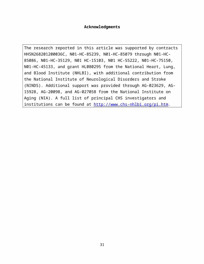
Acknowledgments

The research reported in this article was supported by contracts HHSN268201200036C, N01-HC-85239, N01-HC-85079 through N01-HC-85086, N01-HC-35129, N01 HC-15103, N01 HC-55222, N01-HC-75150, N01-HC-45133, and grant HL080295 from the National Heart, Lung, and Blood Institute (NHLBI), with additional contribution from the National Institute of Neurological Disorders and Stroke (NINDS). Additional support was provided through AG-023629, AG-15928, AG-20098, and AG-027058 from the National Institute on Aging (NIA). A full list of principal CHS investigators and institutions can be found at http://www.chs-nhlbi.org/pi.htm.

22

METHODS APPENDICES*

1 Creation of dependent variables (24)

2 Beta tests of the CHSHLC (30)

3 More about R2 (31)

4 Root Mean Square Error for Training and Validation Samples (34)

5 % of Predictions more than 5 years from the Observed (35)

6 CHS versus MESA (External Validation) (36)

7 List of variables used in Screen 1 of “all the variables in the world” (38)

8 Comparison of Years of Lucid Life to Years of Healthy and Able Life (40)

9 “What if” we had forced additional variables into the predictor? (43)

10 Estimated Number of Users of the Web Application (53)

11 Possible Estimates for persons under 65 (54)

The first 6 appendices were mentioned in the published paper. The remainder represent new research.

23

1

Appendix 1

Creation of Dependent Variables

The main text describes YOL, YHL, YABL, YHABL. These quantities were created as follows.

A variable named YOL_20 was calculated as the number of years that each person (wave) lived during his/her 20 years of follow-up. YHL_20 is the number of years in which she was Healthy. YABL_20 is the number of years in which she was Able. YHABL_20 is the number of years in which she was both Healthy and Able. The outcomes as a group are referred to as “Years_20”.

We needed lifetime values (Years_life). For the 85% of persons who died before 2013, Years_life was known. We estimated the remaining years for the 15% of persons who were still alive in 2013, as follows. Using all waves of data, we regressed Years_20 on baseline age, sex, Healthy and Able (including some transformations). This equation was used to estimate the remaining years. Thus, for a person who was 65 at baseline and still alive 20 years later, the estimated number of remaining years for a person age 85 and of the same sex, Healthy and Able status at baseline was used to generate a random variable from the Poisson distribution with the same mean as that estimate. That random value was then added to Years_20 to provide Years_life. These estimates should have been reasonable, on average.

The resulting lifetime summary variables were named YOL_life, YHL_life, YABL_life and YHABL_life. These were the outcome variables used for the prediction analysis. In the main text, “_life” is dropped, and for instance YHL_life is referred to simply as YHL.

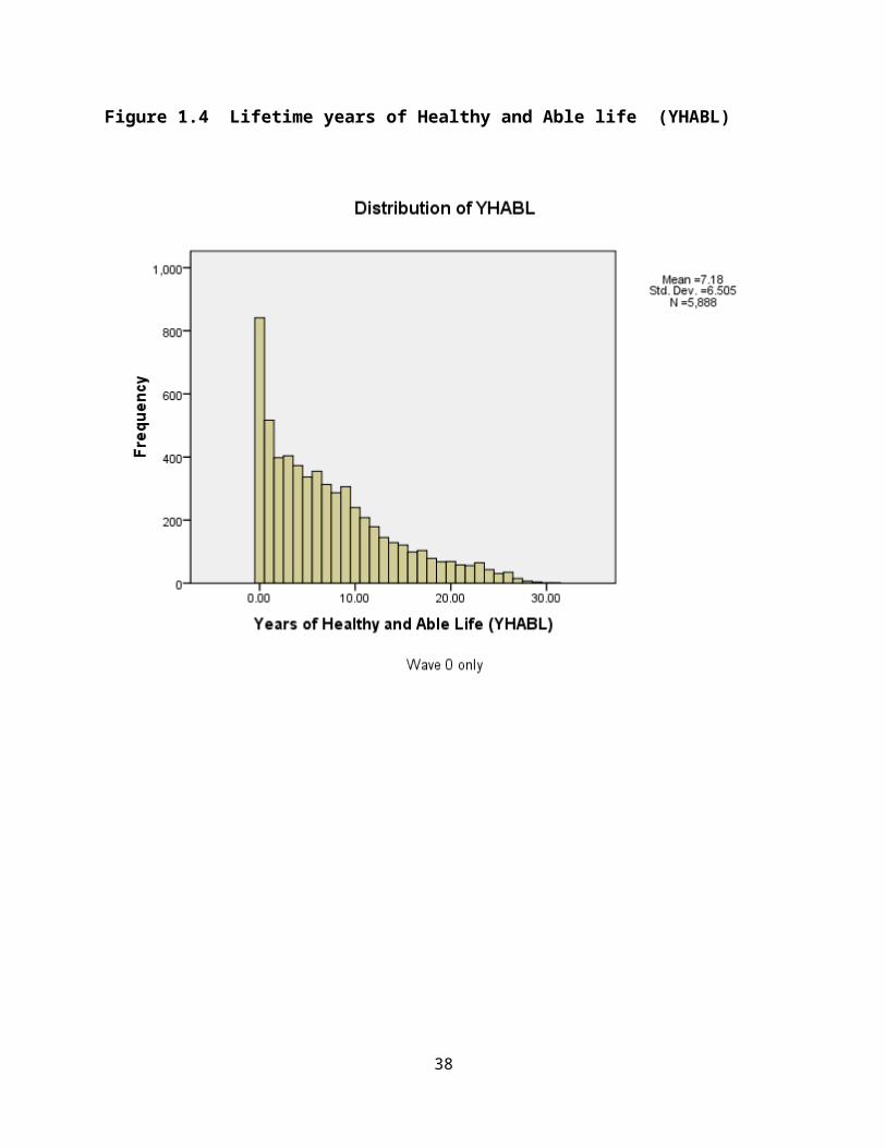
Histograms of the four dependent variables are shown below, for wave 0 only (the true baseline). The histograms have attractive distributions except at year 20.0, for YOL, where too many of the people still alive at year 20 were estimated to survive exactly 20 years. We tried various means to correct this anomaly, but each attempt caused a different problem. The problem may be due to the extrapolation to year 20 that was necessary in some cases. Or perhaps the regression estimates used to extend the data worked less well for YOL. This is the version used, and we believe that the averages of the extensions are reasonable, since they were calculated from real data. They affect only the last few years for 15% of the cases. The histograms for YHL and YHABL are the most attractive. The histogram for YAL (YABL) probably reflects that we had to impute years 10-14 entirely (except for the deaths) because the variable was not collected in a usable form in those years.

It may be surprising that about 800 persons in this (presumably) positively selected sample have no years of healthy and able life (YHABL = 0). At baseline, the here is the

24

distribution of Healthy and Able for those persons. Only 198 were neither Healthy or able; 73 were Healthy but not Able; 364 were Able but not Healthy; and 206 were both healthy and able, for a total of 841. How can people with no YHABL have been both healthy and able at baseline? That is because the graph calls all persons with 0 to .999 as 0. So if they were healthy and able at baseline but because unhealthy and/or unable and/or dead 1 year later, then would have a fraction, and be included in the zero category.

25

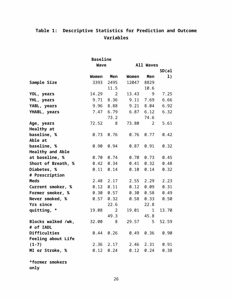
Figure 1.1 Years of Life (life expectancy) (YOL)

26

Figure 1.2 Lifetime years of Healthy Life (YHL)

27

Figure 1.3 Lifetime Years of Able Life (YABL)

28

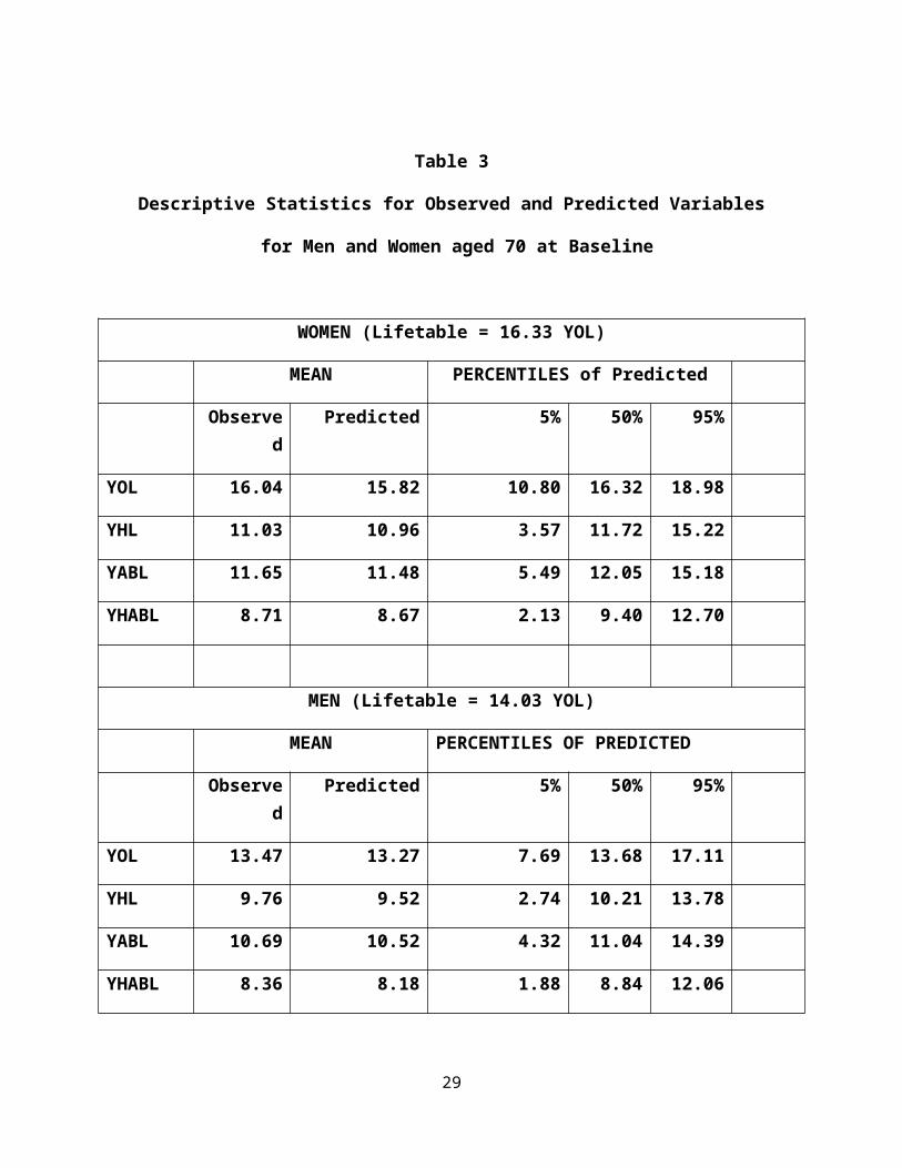
Figure 1.4 Lifetime years of Healthy and Able life (YHABL)

29

Appendix 2

Beta Tests of the CHSHLC

We conducted three waves of beta tests on different convenience samples. A few of the insights gained were mentioned in the main paper. We had intended to make the questions on the CHSHLC identical to those on the 1990 baseline questionnaire. However, beta testers had problems with the wording of some of the questions, felt that there was not enough credit given for walking and length of smoking cessation, etc. More detailed response categories were added for some of the questions.

We believe that the main value of the CHSHLC is that it is well-documented, but beta testers did not usually read the documentation. (The page count for the documentation page is less than 40% of the page count on the main page). As a response, we added more detail to the predictions themselves, to emphasize the amount of possible variability in the predictions.

We originally took a user-friendly tone. However, the beta testers did not seem to treat the CHSHLC seriously, and so we changed the tone to be more serious and professional.

Finally, beta testers usually mentioned their YOL estimate, rather than discussing their YHL and YABL estimates which we thought were a major contribution of this research. We changed the text somewhat to further emphasize the non-mortality outcomes. If older adults are not interested in being healthy and able, then the use of the CHSHLC may be limited, since the U.S. Lifetable is readily available and seemed to be about as accurate as our YOL estimates.

Some users questioned why certain variables were not used as predictors. Some variables were never collect in CHS. Others were ineligible because they could not easily be self-reported. The remainder did not enter because they were not strong predictors after controlling for the variables already in the equation. This is explained in detail in the documentation.

30

Appendix 3,

More about R2

Table 3.1 provides additional R2 information. The top half (first column) is for regression of the predicted value on the observed value ( R2 from .37 to .408). This gives the total R2 including the effect of sex, which doesn’t show up in the sex-specific calculations. The next column shows that a regression with only age and sex and interactions accounts for 22.9% of the variability in R2, 15.6 for YHL, etc. Thus, the CHSHLC explains about 40% of the variability, and on the order of half of the explained variability is due to age and sex.

Appendix Table 3.1

The lower part of the table shows the R2 at each step in the sex-specific regressions. For example, in YOL for women, 21.2% of the variability was explained by age (and log age), which rises to 27.2% when the Healthy and Able variables were added, to .311 when the screen 1

31

variables were added, and to .377 overall. The rightmost four columns show the change in R2 at each step, and the bottom line shows the mean across the four regressions. For YHL for women , 14.5% of the variability is accounted for by age alone, another 18.2% from healthy and able, another 4.7% for the screen 1 variables, and another 2.2% for the screen 2 variables. Averaging across the four equations, for women, Screen 1 and Screen 2 accounted for similar amounts of variability, while for men, the screen 1 variables accounted for twice as much additional variability as the screen 2 variables. A general conclusion is that there were diminishing returns at the four steps.

We might have used a different screening strategy. For example, what if we had not required the same variables to enter in all 8 regressions during the first screening? In Appendix Table 3.2, the first column shows that if alpha = .0001, only 4 to 6 variables would have entered, and they were not always the same variables. The R2 was not much higher than shown in Appendix Table 3.1.

The next columns show what would have happened if we did not require variables to be the same in all 8 regressions, and used an alpha = .01 instead of .0001. Two or three times as many variables entered. The increase in R2 , shown in the final column, however, was quite small. The improvement was on the order of .01 or .02, and there would undoubtedly be considerable slippage due to the large number of variables considered and the lack of restrictions.

We conclude that a different screening strategy would have required a much longer questionnaire, possibly including more variables significant by chance alone, and that this revised strategy not have explained much more variability than the strategy that we used.

32

Appendix Table 3.2

Effects of Alternate Screening Strategies

Alpha = .0001 Alpha = .01

# VARS

ENTEREDR2 # VARS

ENTEREDR2 INCREASE

IN R2

FEMALE

YOL 4 .296 12 .315 .019

YHL 5 .369 10 .380 .011

YABL 5 .347 11 .361 .014

YHABL 6 .377 10 .386 .009

MALE

YOL 4 .298 13 .324 .026

YHL 4 .366 11 .387 .021

YABL 4 .321 13 .346 .025

YHABL 4 .361 12 .386 .025

33

Appendix 4

Root Mean Square Error for Training and Validation Samples

The root mean square error for the two samples is in the following table. For example, RMSE for YOL was 5.8868 in the training sample and 5.9635 in the validation sample, only slightly larger. The RMSE for the validation sample is about .1 years larger than that for the training sample, on the order of 2% larger. This indicates very little slippage or overfitting.

Report

training YOL YHL YAL YHABL

validation sample Mean 5.9635 5.0742 5.5083 4.8278

N 7364 7364 7364 7364

Std. Deviation .00000 .00000 .00000 .00000

training sample Mean 5.8868 4.9314 5.4033 4.6987

N 13512 13512 13512 13512

Std. Deviation .00000 .00000 .00000 .00000

Total Mean 5.9139 4.9817 5.4404 4.7442

N 20876 20876 20876 20876

Std. Deviation .03664 .06824 .05017 .06166

34

Appendix 5

% of Predictions more than 5 years from the Observed

Table 4 in the main paper showed the % of predictions that were within plus or minus 5 years of the observed values. Appendix Table 5.1 shows the % of predictions that were more than 5 years away from the observed values. For example, at age 65, 28% of the Lifetable estimates were 5 years higher than the observed, as were 26% of the YOL estimates, 21% of the YHL estimates, and so on. These percentages became smaller with age. (Those for 90 and above should probably be ignored because of the small sample size at those ages). Appendix Table 5.2 is the % of predictions more than 5 years lower than the observed. It is notable that the % above and below are quite similar. As a simplification, then, we can approximate these quantities from the % data in Table 4, as (100-%)/2. This approximation was used in the CHSHLC.

Appendix Table 5.1

Percent of Predictions more than 5 years higher than Observed

Lifetable YOL YHL YAL YHABL65.00 28 26 21 25 2070.00 25 21 15 18 1275.00 20 17 10 10 680.00 11 12 6 5 385.00 2 6 7 5 490.00 0 9 8 5 595.00 0 0 0 0 0100.00 0 0 0 0 0

Appendix Table 5.2

Percent of Predictions more than 5 years lower than Observed

Lifetable YOL YHL YAL YHABL65.00 32 29 22 24 2170.00 25 23 16 19 1475.00 21 16 12 13 1080.00 15 11 8 6 585.00 10 10 8 5 390.00 2 10 11 7 595.00 0 0 0 0 0100.00 0 0 0 0 0

35

APPENDIX 6

CHS versus MESA (External Validation)

The external validity check applied estimates developed in the CHS data to the MESA data, which began about ten years later than CHS. As MESA had only 10 years of follow-up, we calculated ten-year outcomes, YOL10 and YHL10. We were also restricted to predictor variables available in both CHS and MESA. The means of the outcomes and of the predictors are in appendix Table 6.1. There were 3900 persons 65 and older in MESA as compared with 20876 in the 4 waves of CHS. MESA enrollees had higher YOL and YHL. This is partially explained by the eligibility criteria, as seen in the fact that on average MESA enrollees were younger, healthier, less short of breath, less diabetic, and (by requirement) none had had a previous MI or stroke. Smoking rates were similar, and CHS had slightly lower depression scores (less depressed).

Appendix Table 6.1

Mean of Regression Variables in CHS and MesaExternal Validity Check

20876 39008.54 9.756.45 7.97

74.14 69.64.77 .89

72.72 79.90.37 .14.12 .15.42 .41.11 .09

5.36 7.01.17 .00

SumSample SizeMeanYOL (10)MeanYHL (10)MeanAgeMeanHealthyMeanHealthMeanShort of BreathMeanDiabetesMeanFormer SmokerMeanCurrent SmokerMeanDepressionMeanMI or Stroke

CHS Mesa

For the validation, a regression of YOL10 and YHL10 on these prediction variables was performed in the CHS sample and then applied to the MESA sample. The observed and predicted values in the MESA dataset are shown in Appendix Table 6.2.

36

Appendix Table 6.2

Predicted versus Observed in the MESA sample

YOL10 YHL10

Predicted Observed Predicted Observed

MESA female 9.56 9.80 7.12 7.71

MESA male 8.87 9.42 7.31 7.80

MESA all 9.23 9.62 7.20 7.76

The observed values were close to the predicted values, but were a little higher, on average. For example, for YOL10, MESA females were predicted to average 9.56 YOL but

actually averaged 9.80 YOL. Differences averaged about half a year. That the MESA cohort did a little better than would have been predicted from the CHS data might be taken as evidence that

the CHS estimates in the main analysis will underestimate YOL and YHL for current users. However, prediction equations in the main paper and here have different predictors and different

outcome variables, suggesting it is unwise to over-interpret these apparent biases.

37

Appendix 7

List of variables used in Screen 1 of “all the variables in the world”

The initial screen was based on all of the variables available at baseline. The datafile we used (called ATVITW for All the Variables in the World) was created for a different paper, published in 1999. 18 That paper required all of the variables to be dichotomized, with any coding inconsistencies corrected before dichotomization. Continuous variables were dichotomized at the mean. The process also, unfortunately, lost the variable labels, and the software used at that time required that all variable names be short, and the names were often not very interpretable. Since that time, the baseline files have changed somewhat, and it is not simple to re-attach all of the labels. We chose instead to screen the variables in the ATVITW file to find good predictors and then to attach the labels only to the chosen variables. After the first screening, the full (non-dichotomized) version of each selected variable was used for further analysis.

In the current prediction paper, we kept only those variables with at least 5800 known cases, because a “forward selection” first removes all of the people with missing data on any variable and can result in a very small analysis file. Requiring that 5800/5888 cases of each variable be known allowed resulted in a dataset of 4198 persons for screening 1. Once the variables were selected, the number of complete cases for the final model was much larger (n=5813 persons). Finally, we used only variables that could easily be self-reported by the user of the CHSHLC. This of course removed most of the laboratory results and measurements made in the clinic, in addition to lengthy scales that could not easily be collected in a brief on-line questionnaire. Clearly, other choices could have been made, and might have resulted in different variables being chosen for the calculator.

The variables used in the screen 1 regression are listed in Table 7.1. This listing will probably not be useful to persons who are not CHS investigators. Also note that a few variables are listed more than once (e.g., several variants of age), due to different choices for the coding (original scale and log scale).

38

Appendix Table 7.1

39

Appendix 8

Cognition: Comparison of Years of Lucid Life to Years of Healthy and Able Life.

In addition to concern about their future Health and Ability, older adults also have concern about cognitive decline. CHS did not collect lifetime data on cognition, but it did collect the Modified Mini Mental State Exam (a.k.a. 3MSE) from 1990 to 1999. The original 30-point MSE, with a cutpoint of 23, has 88% sensitivity and 86% specificity to detect dementia, although it is less sensitive to mild cognitive impairment.19 (Other cognition data, collected later, are described below).

We used two approaches to examine how “healthy and able” was related to “Lucid”, defined here as a 3MSE score of 80 or above. We chose the cut-off of 80 because 94% of the CHS enrollees had a score above 80 at baseline. (More specifically, 63% had a score above 89 and another 31% had a score from 80 to 89.) While a score above 80 does not guarantee that a person had no cognitive impairment (the 3MSE is a screener for dementia that is usually followed up by other tests), it does suggest that the person was considered sufficiently lucid to be able to participate in CHS for 3 years.

Two approaches were used. The first used only data from chs year 2 to chs year 11, when the 3MSE was measured for everyone. The second approach used data that were collected later on, but using a different instrument (the telephone interview for cognitive status, or TICS). 20 No cognition data at all were collected in CHS years 12 through 17, or year 19, so that information plus any missing values had to be imputed. We used the general approach given elsewhere 21 with the addition that the “Lucid/not Lucid” dummy variables were post-adjusted during CHS years 12-15 to force the average population value to lie on a straight line drawn from year 11 to year 18, when data were available. (This post-adjustment was probably needed because a large number of persons died in years 12-17, and the imputation method we used tended to over-state the terminal drop in cognition).

Approach 1. Data from CHS years 2 through 11 only.

We used the available information to examine the relationship between Years of Healthy and Able Life (YHABL) and the number of years with a 3MSE score greater than 80 (Years of “Lucid” life (YLUCID)).

We calculated the number of years in which a person was Lucid (had a 3MSE>80) in the 9 years of follow-up available. We compared YLUCID to YHABL, calculated over the same time period, noting how often YLUCID was better (higher), about the same, or worse (lower) than YHABL. Table 8.1 shows the results. The distribution varies by age. YLUCID was

40

greater than or equal to YHABL in all but 8.5% of the cases for ages 65-74. Even at the oldest age, all but 36.8% had YLUCID>YHABL. Over-all, only 13.9% had lower YLUCID less than YHABL.

Table 8.1

Percent where YLUCID is better, same, or worse than YHABL

1 U/S. Lifetable from Social Security Administration: http://www.ssa.gov/oact/STATS/table4c6.htm 2 Fried LP, Borhani NO, Enright PL, et al. The Cardiovascular Health Study: design and rationale. Annals of Epidemiology 1991. 1:263-276.

3 Diehr P, Patrick D, Hedrick S, Rothman M, Grembowski D, Raghunathan TE, Beresford S: Including deaths when measuring health status over time. Medical Care 33:AS164-AS172, 1995. (PMID: 7723444)

4 Diehr P, Patrick DL, Bild DE, Burke GL, Williamson JD: Predicting future years of healthy life for older adults. J Clin Epidemiology 51:343-353, 1998. (PMID: 9539891)

5 Diehr P, Patrick D, Burke G, Williamson J: Survival versus years of healthy life: which is more powerful as a study outcome? Control Clin Trials 20:267-279, 1999. (PMID: 10357499)

6 Diehr P, O’Meara ES, Fitzpatrick A, Newman AB, Kuller L, Burke G. Weight, mortality, years of healthy life and active life expectancy in older adults. J American Geriatric Soc. 2008; 56:76-83. (PMID: 18031486)

7 Hirsch CH, Diehr P, Newman AB, Gerrior SA, Pratt C, Lebowitz MD, Jackson SA. Physical activity and years of healthy life in older adults: results from the Cardiovascular Health Study. Journal of Aging and Physical Activity 2010; 18:313-334. (PMID: 20651417)

8 Diehr P, Thielke S, O’Meara E, Fitzpatrick A, Newman A. Comparing Years of Healthy Life, Measured in 16 Ways, for Normal Weight and Overweight Older Adults. Journal of Obesity 2012 (on-line only); doi:10.1155/2012/894894. http://www.hindawi.com/journals/jobes/2012/894894/ 9

? Locke E, Thielke S, Diehr P, Wilsdon AG, Graham Barr R, Hansel N, Kapur VK, Krishnan J, Enright P, Heckbert SR, Kronmal RA, Fan VS. Effects of respiratory and non-respiratory factors on disability among older adults with airway obstruction: the Cardiovascular Health Study. COPD 10: 588-596. 2013.

10 Longstreth , Diehr PH, Yee L, Newman AB, Beauchamp N. Brain imaging findings in the elderly and years of life, healthy life, and able life over the ensuing 16 years: the Cardiovascular

41

Better, Same, Worse * agecat10 Crosstabulation

agecat10

65-74 75-84 85-95 95+ Total

Better, Same, Worse yhabl < ylucid 54.4% 56.2% 52.3% 39.3% 54.8%

yhabl = ylucid 37.0% 30.1% 22.9% 23.9% 31.3%

yhabl>ylucid 8.5% 13.7% 24.8% 36.8% 13.9%

Total 100.0% 100.0% 100.0% 100.0% 100.0%

Health Study. JAGS 62: 1838-1843, 2014.

11 Diehr, Paula, "Methods for Dealing with Death and Missing Data, and for Standardizing Different Health Variables in Longitudinal Datasets: The Cardiovascular Health Study" ( July 2013). UW Biostatistics Working Paper Series. Working Paper 390. http://biostats.bepress.com/uwbiostat/paper390

12 Protocol for the Multi-Ethnic Study of Atherosclerosis (MESA). http://www.MESA-nhlbi.org/publicDocs/Protocol/MESAProt000225-updated.doc

13 Diehr P, Patrick DL, Spertus J, Kiefe CI, McDonell M, Fihn SD. Transforming self-rated health and the SF-36 Scales to include death and improve interpretability. Medical care 39:670-680, 2001. (PMID: 11458132)

14 Lumley T, Diehr P, Emerson S, Chen L. The importance of the normality assumption in large public health data sets. Annual Review of Public Health 23:151-169, 2002. (PMID: 11910059)

15 MacIver J1, Rao V, Delgado DH, Desai N, Ivanov J, Abbey S, Ross HJ. Choices: a study of preferences for end-of-life treatments in patients with advanced heart failure. J Heart Lung Transplant. 2008 Sep;27(9):1002-7. Epub 2008 Jul 26.

16 Diehr PH, Thielke SM, Newman AB, Hirsch CH, Tracy R. Decline in health for older adults: 5-year change in 13 key measures of standardized health. J Gerontol A Biol Sci Med Sci. 2013 May 10. [epub ahead of print] doi:10.1093/gerona/glt038 [PMID:23666944]

17 Diehr P, Williamson J, Burke G, Psaty B. The aging and dying process and the health of older adults. Journal of Clinical Epidemiology 55:269-278, 2002. (PMID: 11864798)

18 Diehr P, Patrick D, Burke G, Williamson J: Survival versus years of healthy life: which is more powerful as a study outcome? Control Clin Trials 20:267-279, 1999. (PMID: 10357499)

19 Lin JS, O’Connor E, Rossom RC, Perdue LA, Burd BU, Thompson M, Eckstrom E. Screening for cognitive impairment in older dults: an evidence update for the U.S. Preventive Services Task Force. Rockville (MD): Agency for Healthcare Research and Quality (US); 2013 Nov.

42

A crude multi-state lifetable calculation

We used the numbers in Table 8.1 for a crude calculation. From the table, for persons starting out at age 95+, 36.8% have YLUCID<YHABL, and 63.2% have YLUCID >YHABL. There were few people at this age at baseline, and this number is unreliable.

Now consider 100,000 women starting at age 85-94. By the tabled numbers (assuming dementia data are similar for men and women), 24.8% will have YLUCID<YHABL in the next 10 years, leaving 75,200 with YLUCID >YHABL. Of these, 68.943 would die in the 10 year period, meaning that YLUCID >YHABL for all of them. Of the 6527 still alive, according to the table, 2302 would have YLUCID<YHABL, and 3954 would have YLUCID >YHABL. Thus, the total of the original 100,000 who had YLUCID >YHABL throughout their remaining lives is 68,943 + 3,954 = 72, 897, or about 73%. Through increasingly tedious calculations, we estimated the % for whom YLUCID >YHABL throughout their remaining lives at younger ages. Table 8.2 shows that for about 63% to 74% of the persons, depending on initial age, YLUCID >YHABL.

Report No.: 14-05198-EF-1. U.S. Preventive Services Task Force Evidence Synthesis, formerly Systematic Evidence Reviews.

20 Arnold AM, Newman AB, Dermond N, Haan M, Fitzpatrick A. Using telephone and informant assessments to estimate missing Modified Mental-Mental State Exam scores and rates of cognitive decline. The Cardiovascular Health Study. Neuroepidemiology 2009:33;55-65.

21 Diehr, Paula, "Methods for Dealing with Death and Missing Data, and for Standardizing Different Health Variables in Longitudinal Datasets: The Cardiovascular Health Study" ( July 2013). UW Biostatistics Working Paper Series. Working Paper 390. http://biostats.bepress.com/uwbiostat/paper390

43

Table 8.2

Crude estimate of lifetime percentage with YLUCID >YHABL

Age

Wome

n

Men

70 73 7780 74 7790 73 74

100 63 63

These calculations required several strong assumptions. First, we used age-specific mortality rates, but combined dementia data. (Results were slightly better for men because they died sooner). Second, we assumed that mortality and the onset of dementia were statistically independent. Third, we assumed that the percentages in Table 8.1 were for a decade when they were really only for 9 years. And finally, we assumed that a single decade where YLUCID<YHABL cancelled out any positive results in any other decade. The results in Table 8.2 clearly should not be over-interpreted, but they do justify the statement in the CHSHLC that YLUCID is usually greater than YHABL.

Thus, based on these numbers, the great majority of older adults should have more lifetime YLUCID than lifetime YHABL. This was true for 100-37 = 63% of persons starting at age 95, and that number will be higher for persons starting at younger ages. Therefore, it is reasonable to assume that n the years in which a person is both healthy and able she will also be Lucid. This is consistent with other research showing that cognition declines at a slower rate than do self-rated health and ADL abilities.

Approach 2. Using the observed and imputed longitudinal 3MSE and TICS data

for 20-year cognition.

We used the 20-year longitudinal cognitive data to calculate YLUCID20, which is the number of years (in the 20 years after baseline) when the person had a 3MSE score (either real, estimated from TICS, or imputed) >80. We then compared YLUCID20 to YHABL20. For 75%

44

of the CHS enrollees, YLUCID20 > YHABL20. We take that to mean that YLUCID > YHABL for most people, and that because of that, it is usually safe to use YHABL to plan for the future.

Appendix 9

“What if” we had forced additional variables into the predictor?

Introduction

The CHS Healthy Life Calculator (to be found at https://healthylifecalculator.org/) was created by screening all of the appropriate baseline variables, and choosing the best predictors. Clearly, there are many ways that “appropriate” and “best” could be defined. Here are the restrictions we used:

a. Only variables that could easily be answered by a person in a short questionnaireb. Only variables that were observed for 5800 or more CHS enrollees (98.5%)c. Only variables that were highly statistically significant (p<.0001 for stage 1, p<.01 for

stage 2) for all eight of the outcomes: YOL, YHL, YAL, YABL for men and for women.

These exclusions thus removed from consideration all of the lab and physical exam results, as well as any scales that were calculated from lengthy questionnaires, or variables that performed differently for men and women. Here is what happened when we relaxed some of those restrictions.

Methods

We chose the additional variables to check for eclectic reasons, including whether early CHSHLC users had asked about them, whether they had been used in Mini Jacob’s paper, whether they had been excluded from the original analysis as too hard to answer, or just for our own curiosity. Variables that were binary were used as-is. Variables with more than two categories were dichotomized to indicate approximately the “top third” of the distribution. (The actual proportions are shown in Table 9.0a and 9.0b.)

For each new variable, we ran 8 regressions, for 4 outcomes (YOL, YHL, YAL, YHABL) and both genders. The dependent variable was the residual of the CHSHLC (observed minus estimated). We computed a regression with no constant term, so that the regression coefficient would correspond to the adjustment to the predicted value that could be reasonable for this variable.

The regression coefficients (the increases) and their p-values are shown in Tables 9.1 – 9.3. To aid in discussion, we highlighted coefficients > .5 years (6 months) and p-values < 0.01.

45

Results

0.0 Descriptive statistics

Tables 9.0a and 9.0b give descriptive statistics for all of the variables in this analysis, separate for women and for men. The N is the number of known observations for each variable. The first four variables are the dependent variables, and the remainder are the new variables that are examined here (all coded 0/1). The mean of the binary variables can be interpreted as the proportion who have that characteristic; i.e., 30.21% of the women were in the KCAL_high group (defined below).

Table 9.0A Female Descriptive Statistics

Descriptive Statistics

N Minimum Maximum Mean Std. Deviation

YOL_LIFE 3393 .25 28.87 15.2669 7.66468

YHL_LIFE 3393 .00 26.11 9.7661 7.01442

YAL_LIFE 3393 .00 27.01 10.7513 7.52845

YHABL_LIFE 3393 .00 25.38 7.9309 6.79222

KCAL_HIGH 3032 .00 1.00 .3021 .45925

BLOCKS_HIGH 3393 .00 1.00 .0754 .26415

healthyeating 3393 .00 1.00 .2756 .44687

OBESEBASE 3393 .00 1.00 .2293 .42044

chfbase 3393 .00 1.00 .0239 .15267

anysubth 3393 .00 1.00 .6281 .48339

depscr05 3386 .00 1.00 .4616 .49860

diag01 3387 .00 1.00 .1411 .34820

Lucid 3M > 90 3393 .00 1.00 .6110 .48760

brach 3329 .00 1.00 .4533 .49789

glu44 3337 .00 1.00 .2298 .42080

black 3393 .00 1.00 .1712 .37677

anyapoe4 3018 .00 1.00 .2545 .43564

Valid N (listwise) 2632

46

Table 9.0B Male Descriptive Statistics

Descriptive Statistics

N Minimum Maximum Mean Std. Deviation

YOL_LIFE 2495 .25 27.52 12.1757 7.20514

YHL_LIFE 2495 .00 25.21 8.3924 6.54287

YAL_LIFE 2495 .00 25.79 9.4018 6.95087

YHABL_LIFE 2495 .00 24.57 7.2349 6.32798

KCAL_HIGH 2294 .00 1.00 .3766 .48465

BLOCKS_HIGH 2495 .00 1.00 .1427 .34982

healthyeating 2495 .00 1.00 .2593 .43835

OBESEBASE 2495 .00 1.00 .1555 .36246

chfbase 2495 .00 1.00 .0333 .17937

anysubth 2495 .00 1.00 .7431 .43702

depscr05 2492 .00 1.00 .3258 .46878

diag01 2491 .00 1.00 .1453 .35250

Lucid 3M > 90 2495 .00 1.00 .5603 .49645

brach 2471 .00 1.00 .4379 .49623

glu44 2471 .00 1.00 .2906 .45412

black 2495 .00 1.00 .1375 .34442

anyapoe4 2222 .00 1.00 .2516 .43402

Valid N (listwise) 2007

47

1.0 Table 9.1 shows the results for 4 variables related to exercise and diet. Exercise was already represented in the CHSHLC by “blocks walked” but some users did not think it gave enough credit for serious exercisers. No dietary variables were screened for the published calculator.

KCAL_high (from KCAL, total KCALS of physical activity) is a variable that indicates being in the top third of energy expenditure, and includes more activities than walking. The first entry in Table 9.1 shows that the coefficient of YOL for men was 0.59 years, and the p-value was .002. That is, a reasonable “fix” for a man who believed he was in the top tertile of energy expenditure would be to add .59 years (7 months) to the calculator estimate. Values >.5 years or p<.01 are highlighted throughout. Note that for men, the coefficient was always >.5 and the p-value was always less than .01, suggesting that a highly active man could probably justify adding about half a year to each of his calculator estimates. There was no evidence that women needed any adjustment, because their coefficients were small and the p-values non-significant. The gender difference may be because in 1990 women mainly exercised by walking, and/or did not exercise as much as men.

Blocks_high is a binary variable that is 1 if the person walked more than 100 blocks per week (the calculator limit was 72 blocks), and 0 otherwise. Although Blocks was already in the calculator, it was used there on the log scale, so that there was a diminishing return on walking built into the model. (The log scale was chosen to reduce the effect of outliers, and was also a slightly better predictor than blocks measured on the linear scale.) Coefficients in table 9.1 were not large, were actually negative for women, and were never significantly different from zero. No adjustment is indicated, for men or for women.

HEI_high refers to being in the top third of the healthy eating index. This variable was not originally screened, because it was not available for cohort 2. In Mini’s paper22, HEI was significantly related to YAL/YOL% (% of remaining life that was Able). Table 9.1 shows that HEI_high would be a good additional predictor only for YHL for women. (Mini’s analysis controlled for potential confounders, while the CHSHLC controlled for the variables that were the best predictors.) This could suggest adding half a year of YHL for women who “eat right”, but the inconsistency of the results suggests that this is most likely a chance finding.

Obesity was not specifically considered in screening for the original calculator variables, although the continuous BMI value was screened. Here, we screened a specific indicator for obesity. Table 9.1 shows that obese persons might reasonably decrease their YAL and YHABL predictions by about half a year. In a second analysis, we defined obesity by recalled BMI at age 50 , to account somewhat for weight loss due to illness.23 This different definition made no difference for men, but

22 Jacob ME, Yee LM, Diehr PH, Arnold AM, Thielke SM, Chaves HM, Del Gabbo L, Hirsch C, Siscovick D, Newman, AB. Can a healthy lifestyle compress the disabled period in older adults? JAGS 2016. J Am Geriatr Soc. 2016 Sep 7. doi: 10.1111/jgs.14314. [Epub ahead of print].

48

seemed to be meaningful for women. Again, Obese 50 would not have satisfied our original requirements, but if we had allowed different variables for men and women it might have entered for women. The coefficients of the significant variables are large enough to be interesting.

23 Yu E, Ley SH, Manson JE, Willett W, Satija A, Hu FB, Stokes A. Weight history and all-cause and cause-specific mortality in three prospective cohort studies.

49

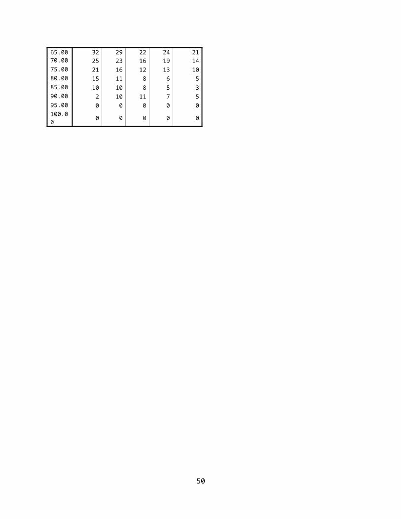
Table 9.1

Exercise and Diet

KCAL_HIGH YOL YHL YAL YHABLM 0.59 0.002 0.69 0.000 0.61 0.001 0.69 0.000F 0.00 0.982 0.02 0.902 0.11 0.557 0.06 0.717

BLOCKS_HIGH YOL YHL YAL YHABLM 0.15 0.627 0.06 0.816 0.02 0.940 0.13 0.607F -0.54 0.139 -0.06 0.877 -0.53 0.131 -0.21 0.515

HEI_HIGH YOL YHL YAL YHABLM 0.21 0.363 0.29 0.149 0.18 0.402 0.21 0.269F 0.37 0.058 0.55 0.003 0.15 0.402 0.33 0.052

OBESE YOL YHL YAL YHABLM 0.08 0.794 -0.28 0.284 -0.66 0.018 -0.55 0.026F -0.05 0.818 -0.34 0.104 -0.66 0.001 -0.60 0.001

OBESE 50 YOL YHL YAL YHABLM -0.36 0.304 -0.36 0.260 -0.67 0.045 -0.46 0.121F -0.76 0.015 -0.49 0.109 -1.04 0.000 -0.66 0.016

50

2.0 The variables in Table 9.2 were originally either unscreened or were screened but failed.

CHFbase was originally screened and did not enter then. (Some other heart variables were included in the calculator). In the current check, although the coefficients are quite large and the signs make sense for all outcomes, there was only a “significant” result for YOL. The user who asked us about his CHF said that medication suppresses most of his symptoms, and so he had a fairly good prognosis for YHL and YAL based on the calculator. Perhaps the results are due in part to the small number of CHS enrollees who had CHF at baseline (2% of women, 3% of men). It might have been wise to include CHF with the other heart variables in the calculator, for completeness.

ANYSUBTH (subclinical disease from the baseboth variables, not including echo) notes whether a person had any subclinical findings (about 70% did). ANYSUBTH was not originally screened because the user would not have been able to answer this question. In Table 9.2 ANYSUBTH is always a statistically significant predictor, but the coefficients (and thus the recommended amount of adjustment) would all be less than half a year.

Depression (CESD scale) was not originally screened because it required a lengthy questionnaire. The calculator did, however, include a rating of the user’s feeling about her life as a whole, from Terrible to Delighted, which was correlated with the CESD (not shown). Table 9.2 shows the results of being in the highest (worst) third of the responses. The results are not very consistent, but YHABL might reasonably be decreased by about half a year for people in the worst third of the depression scale.

Diag01 is a history of previous cancer (currently being treated for cancer was a baseline exclusion for CHS). Table 9.2 suggests that it may be reasonable to decrease scores for women (but not for men) by about 6 to 12 months. The inconsistency of the findings by sex is unexplained.

Lucid here indicates a baseline 3MSE of 90 or higher (we used a threshold of 80 elsewhere). We chose a high threshold to ensure that there were enough people in the lower group for this analysis. Scores below 90 do not necessarily indicate dementia, especially since all CHS enrollees were lucid enough to participate in the demanding baseline clinic visits. Lucid was significantly associated with YHL and YHABL, although the coefficient is only about 3 months. The result is consistent by sex, but does not hold as strongly for YOL or YAL.

51

Table 9.2

Conditions not in the Calculatorchfbase YOL YHL YAL YHABLM -1.47 0.019 -0.58 0.306 -0.78 0.191 -0.40 0.456F -1.55 0.018 -0.53 0.403 -0.64 0.303 -0.03 0.962

ANYSUBTH YOL YHL YAL YHABLM -0.47 0.000 -0.39 0.001 -0.35 0.006 -0.30 0.009F -0.46 0.000 -0.40 0.001 -0.35 0.004 -0.35 0.002

DEPRESSION SCORE YOL YHL YAL YHABLM 0.05 0.785 -0.37 0.040 -0.25 0.183 -0.46 0.006F -0.04 0.809 -0.46 0.001 -0.30 0.035 -0.50 0.000

diag01 YOL YHL YAL YHABLM -0.10 0.737 0.10 0.718 -0.12 0.680 0.12 0.625F -0.99 0.000 -0.65 0.013 -0.80 0.002 -0.55 0.021

lucid 3MSE > 90 YOL YHL YAL YHABLM 0.27 0.073 0.36 0.008 0.30 0.037 0.35 0.007F 0.29 0.026 0.33 0.008 0.29 0.016 0.28 0.014

52

3.0 A few more variables

In Table 9.3, BRACH (average brachial pressure for AAI) was found to be one of the best predictor variables in this new analysis; it was originally excluded because it couldn’t be self-reported. Noting whether the person was in the top 45% of BRACH (coded from a previous analysis) could have been a meaningful additional factor (coefficient was about 9 months for men, but not for women).

GLU44 (baseline glucose in about the top quarter) was a strong predictor which was not originally screened because people would not be able to self-report it. Glucose was meaningful here, even though self-reported diabetes was already in the calculator. Perhaps GLU44 reflects untreated diabetes. There were consistent results for men and women, although YHL was not as strongly statistically significant for women. A decrease of 9 months for all outcomes would be reasonable.

APOE allele 4. This variable represents “any allele 4”, and combines APOE categories 3 (2,4), 5 (3,4) and 6 (4,4). It is the genetic variable measured on the most CHS enrollees. The significance level was never <.01, and the coefficients were only on the order of 3 months. This genetic variable would not have made any difference to the calculations.

Table 9.3

Other variablesBRACH YOL YHL YAL YHABLM -0.75 0.000 -0.80 0.000 -0.73 0.000 -0.73 0.000F -0.37 0.014 -0.32 0.030 -0.38 0.008 -0.33 0.015

glu44 YOL YHL YAL YHABLM -0.77 0.000 -0.80 0.000 -0.74 0.000 -0.77 0.000F -0.55 0.010 -0.54 0.009 -0.53 0.009 -0.44 0.018

APOE 4 YOL YHL YAL YHABLM 0.32 0.023 0.28 0.024 0.30 0.021 0.26 0.026F 0.22 0.071 0.22 0.064 0.24 0.038 0.19 0.085

53

4.0 SES Variables

Socio-economic status is often a meaningful correlates of health and activity. To be sure we hadn’t missed anything, we re-considered race, income, and education. Table 9.4 shows that being black and being a high school graduate were almost never meaningful or statistically significant. Low income (defined as <$35k, which Is the bottom 2/3), was meaningful and significant for men, but not for women. The coefficients for men were a decrease of about 6 months for being in the lower 2/3. This variable did not meet the criteria because it was not relevant for women, but one could justify a post-adjustment for men only. It might have been better to use a smaller low income group, assuming that the adjustments would be even larger.

Table 9.4

SES VARIABLES

BLACK YOL YHL YAL YHABLM -0.06 0.857 -0.43 0.132 0.04 0.892 0.59 0.018F -0.11 0.640 -0.24 0.309 -0.43 0.051 -0.03 0.962

LOW INCOME YOL YHL YAL YHABLM -0.47 0.003 -0.56 0.000 -0.53 0.000 -0.57 0.000F -0.19 0.135 -0.24 0.053 -0.30 0.012 -0.31 0.006

HSGRAD YOL YHL YAL YHABLM 0.21 0.130 0.24 0.051 0.22 0.092 0.25 0.033F 0.02 0.861 0.09 0.421 0.04 0.745 0.08 0.455

Conclusions

Many CHS variables were excluded from the CHS Healthy Life Calculator because of the selection requirements listed in the introduction to this appendix. We examined whether a selection of additional variables could have made a meaningful and significant improvement to the CHSHLC.

Most of the variables checked would not have contributed in a meaningful way to the Healthy Life Calculator, which is an encouraging finding for the calculator. Based on this analysis, it might have been reasonable to adjust the calculator results for KCAL, Obesity, ANYSUBTH, Brach, and Glu44, if

54

there were any easy way for people to self-report these variables . Their coefficients were meaningful (>.5 years) and statistically significant (p<.01), though not always for both sexes. It isn’t clear, however, how we could have included them in a user-friendly way.

Some preliminary work (not shown) found that the R2 values for prediction were not much higher when the larger set of variables (including those not previously allowed) was screened. There seems to be a natural limit of about 0.4 for R2. This would suggest that adding more variables would not make a meaningful change in the variance of the prediction.

It may be surprising that some of these variables, known from other studies to be strong determinants of health, did not enter the calculator. It may be helpful to think of determinants of health as distal or proximal. The distal variables, such as SES, often exert a causal effect on the proximal variables, such as diabetes. Once the proximal variables are included in the prediction equation, the distal variables often have much less effect.

Three of the four outcomes (all but YOL) were based on self-ratings of health or function. Perhaps that explains why the new, non-self-rated variables did not add much to the predictions.

In nearly all cases, the new variables checked would not have improved the calculator. This suggests that the methods used to choose predictor variable were acceptable.

55

Appendix 10. Estimated number of users of web application.

How can we measure the success of the dissemination? Citations of the paper will provide one measure, but only for how well it reached researchers. The tiny print at the bottom of the web page as of 4-5-2017 said:

This page has been viewed : 11999 times. The Calculator has been used 70 times with 10 attempts with missing data

Most of the accesses are from “robots” which index and re-index the page for various search engines. A crude estimate of the total uses at that time is 325 + 70. (The 325 is the estimate for the earlier period, and is probably an underestimate because this was the time of maximum promotion). About 3.3% of the total views are actual uses.

We didn’t count the actual uses (number of times someone used the Calculate button) until later, when the previous number of accesses was 9870 (P). On April 5, 2017 we had 11999 cumulative accesses (C ), and 70 “uses” (U) from the 11999-9870=2129 new accesses, or put another way, only about 3.3% of the views represented actual uses in this second period. A simple estimate for the total usage (including the earlier period) is 70 + (70/2129)*9870 = 70 + 325 = 395). (Algebraically, estimated total usage to date is UC/(C-P), referring to Uses, Cumulative count, and Previous count, respectively). Previous usage is probably higher than 325 because of all the promotion we did during the first period, meaning that 70/2129*9870 is probably too low for the first period. Perhaps total usage is 500-ish to date. If we assume that 3.3% is correct for the first period, then we can simplify the estimate to Total uses = U + ~325.

On 3-27-2017 we had 50 uses. OnApril 5 (8 days later), we had 70. Perhaps our steady state will be (70-50)/8 per day, or 2.5 uses per day. On April 17, we had 95 uses, 95 +”325”=420 uses. Or, UC/(C-P) = 95*12444/(12444-9870) = 459. On 6-1-17 (71 days later), the numbers are 14322 and 142, respectively. 14322*.033 = 473 total; (142-50)/71 = 1.3 extra uses per day since the counter was added;C = 14322, U = 142, P = 9870, UC/(C-P) = 142*14322/(14322-9870)=456.

The number of uses are increasing, but only gradually, unless we come up with another dissemination approach. Suggestions are welcome.

56

Appendix 11 Estimates for persons younger than 65

What can we tell a younger person, say at age 60? Strictly speaking, we should not give any estimate because we have no data for persons under 65. On the other hand, it may be reasonable to extrapolate the equations a little beyond the range of the data. Age is represented in the prediction equations by a linear and a logarithmic term, and so should not behave badly a little outside the range of data as, for example, a quadratic term might.

We consider two possible approaches. The simplest would be to calculate the estimates for age 65 and then add 5 years to each one. If the person is healthy and able at age 65, he is likely to have been the same at age 60. (The reverse is not true, unfortunately, because a person’s condition may decline in the 5 years to reach age 65.) The “add 5” approach is likely to be an over-estimate. The second approach is to apply the equations for age 60. That is not possible in the online version of the calculator (age limited to 65+), but there are spreadsheets for males and females available at

http://faculty.washington.edu/pdiehr/blank_female.xls and

http://faculty.washington.edu/pdiehr/blank_male.xls .

Consider a woman who is 60 and is like “Mary” above, having the best possible answer for everything in the questionnaire.

The 65 and add 5 approach gives the numbers in columns 1 and 2 of table 11.1. The spreadsheet for female, for the same person at age 60, gives the results column 3. Note that, as expected, the “add 5” estimates were about a year higher than the “extrapolate to 60” estimates (column 4). Table 11.2 gives similar results for men in perfect health, with the difference in the two estimates about a year and a half. It might be interesting to make these comparisons for sicker people, but we have not done so.

The two estimates are based on different assumptions. Both assume that the regression equations are appropriate at age 65. The “add 5” method assumes that the person’s health will not change between age 60 and 65, and so may over-estimate. The “spreadsheet” method assumes that the equations can be extrapolated a few years outside the range of the data. Based on the similarity of the results, the “add 5” method may be simple and reasonable for persons in perfect health at age 60.

57

Table 11.1

Comparison of Estimates for Age 60, for a woman in perfect Health

Age 65 “add 5” Age 60 from spreadsheet

Add 5 minus spreadsheet

YOL 23.6 28.6 27.6 1.0

YHL 20.0 25.0 24.2 0.8

YABL 20.4 25.4 25.3 0.1

YHABL 17.3 22.8 21.2 1.6

Table 11.2

Comparison of Estimates for Age 60, for a Man in perfect Health

Age 65 “add 5” Age 60 from spreadsheet

Add 5 minus spreadsheet

YOL 21.0 26.0 24.5 1.5

YHL 17.8 22.8 21.2 1.6

YABL 18.6 23.6 22.6 1.0

YHABL 15.8 20.8 19.3 1.5

58

We performed a similar exercise to estimate the years for a person age 50. This seems quite dangerous, since 50 is 15 years below the range of the data. As shown in tables 11.2 and 11.3, some of the discrepancies between the estimates are larger, and for women the spreadsheet estimate is sometimes higher than the “add 15” estimate. The patterns are not the same for men and women. This does seem too dangerous.

Table 11.3

Comparison of Estimates for Age 50, for a woman in perfect Health

Age 65 “add 15” Age 50 from spreadsheet

Add 5 minus spreadsheet

YOL 23.6 38.6 37.8 .8

YHL 20.0 35.0 35.7 -.7

YABL 20.4 35.4 39.3 -3.9

YHABL 17.3 32.3 32.5 -.2

Table 11.4

Comparison of Estimates for Age 50, for a Man in perfect Health

Age 65 “add 15” Age 50 from spreadsheet

Add 5 minus spreadsheet

YOL 21.0 36.0 33.2 2.8

YHL 17.8 32.8 30.7 2.1

YABL 18.6 33.6 33.6 0

YHABL 15.8 30.8 28.8 2

59

60

References

61