Christina Clark & Jingkang GaoORF 467 Fall 2012

MyCity Final Report

The City of Pension Heaven: Land Use Characteristics

Character of Pension Heaven

Pension Heaven, a retirement utopia, is a self-sustaining city of population 250,000. The city sits on a square plot of land of size 102.4 square miles, and it is divided into 75 rectangular zones (TAZs) of various sizes, 10 of which are undeveloped (open space and lakes) and 65 are developed.

An unzoned river runs diagonally through the city. There are four zones for lakes; the largest lake occupies 2.5 square miles and the other three lakes are 0.6 square miles in size. Each of the small lakes borders an open space zone. The total area of water (river and lakes) is 14.2 square miles. The city also contains 14 square miles of open space, most of which border the edges of the city. Thus nearly 30% of the city is undeveloped.

Residential areas occupy about a third of the city and they are classified as light residential (~9%), medium residential (~17%), and heavy residential (~9%).

Six zones allocated for education include one research university that does not provide housing to students, two K-8 school districts, two high school districts, and one private day school. The university is located between a strip of open land and the largest lake, which are utilized for university athletic events. Each school district borders at least one residential zone.

There is an airport along the northern border of Pension Heaven. The net population flow for the airport is zero. The airport occupies 4.8 square miles, which is based on a city of comparable size, St. Paul, MN, which has population 290,000 and an airport of size 5.3 square miles.

One large park sized 1.4 square miles (comparable to Central Park, 1.3 square miles) borders a lake near the center of the city. A much smaller park is located in the middle of a residential district in the eastern part of the city.

A football stadium (capacity 100,000) and soccer stadium complex (capacity 100,000)—the complex includes the stadiums and surrounding entertainment and retail as well as parking—is located along the western edge of the city next to the large lake. A baseball stadium (capacity 40,000) and basketball/hockey arena (capacity 20,000) complex (including surrounding parking and retail) is located on the northeastern corner of the city. These sports complexes would be excessive for a normal American city of 250,000 but appropriate for a retirement city where the elderly have the time and financial means to attend sporting events almost daily.

The center of the city consists of a town hall zone—which includes the town hall and other government office buildings—as well as a large retail zone, professional office zone, and light commercial zone. Our public buildings include other types of government office buildings, police stations, and fire stations.

Most industrial zones (total area of about 5 square miles) are located along the river or in the outskirts of the city. Industrial zones include not only factories and plants but also hospitals.

Land Use Map

Zone Information

Summary Tables of Land Use

Demographics and Quality of Life

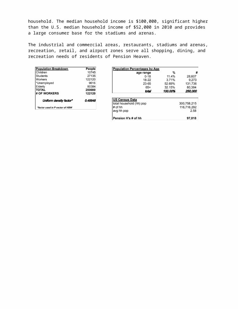
As previously stated, Pension Heaven is a retirement city. A very large portion of the population consists of retirees (we define retires as people age 65 or older), and the working population (we define working population as age 22-65) is much older than the average working population in the United States. Our workers bear children at the same rate as the American population as a whole but since they are older most children no longer live with their parents. Thus the under-18-population ratio (11% of Pension Heaven population) is much lower than that of the entire American population (about 30%); and the over-65-population ratio (32%) is much larger than that of the entire American population (13%), hence the city is named Pension Heaven. 52% of the population in Pension Heaven is female. Pension Heaven attracts the elderly because of the small children population in that local taxes for education are very low compared to other cities.

The population break down and age breakdown correspond as the following. Children population is the same as the under 5 population. Student population consists of the 5-18 population (all 5-18 people attend school) and 9273 university students. Workers include the 18-65 population minus the 9273 university student population and the 9616 unemployed population. *We define our unemployed population not as people seeking work but cannot find work, but as anyone between 18 and 65 who is not working. Thus our unemployment rate cannot be compared to the usual unemployment rates of other cities; it would be much lower (very close to zero) if we defined unemployment as those seeking work but cannot find it.

Workers in Pension Heaven work exclusively in Pension Heaven, and students attending all schools reside in Pension Heaven. Residential density varies from 4,456 per square mile in light residential zones (suburban-like areas) to 10,850 per square mile in heavy residential zones. In Pension Heaven there are no workers in any residential zone.

The population per household number is consistent with that of the 2010 U.S. census. Pension Heaven has 97,018 households; on average each household has 2.58 people. Although Pension Heaven is not similar to the U.S. population in age distribution, the larger number of retirees (who are more likely to be married, thus increasing number of people per household) offsets the small number of children per household. The median household income is $100,000, significant higher than the U.S. median household income of $52,000 in 2010 and provides a large consumer base for the stadiums and arenas.

The industrial and commercial areas, restaurants, stadiums and arenas, recreation, retail, and airport zones serve all shopping, dining, and recreation needs of residents of Pension Heaven.

Demand for Transportation: Trip Generation

Generating the Production and Attraction Vectors1

Home-Based Work (HBW) P&A VectorsProduction: this vector equals the corresponding zone’s residential population multiplied by the uniform distribution constant (since an assumption we must make is that the home-to-work departures are uniform across all zones). This constant was calculated by dividing the total number of workers by the total population.Attraction: this vector must equal the number of workers in each corresponding zone.

Work-Based Home (WBH) P&A VectorsProduction: because 80% of workers go home after work, this vector equals 0.8 multiplied by the total number of workers in each corresponding zone.Attraction: this vector therefore must equal 80% of workers that came from the residential zones. In other words, this equals 0.8 multiplied by the HBW production vector.

Home-Based School (HBS) P&A VectorsProduction: just as we calculated the HBW production vector, this HBS production vector also is uniformly distributed across the residential zones. Therefore, it equals each zone’s residential population multiplied by this uniform distribution constant. The constant was calculated by dividing the total number of students by the total population.Attraction: this attraction vector equals the set number of students in each school zone, as dictated in our Student Breakdown.

School-Based Home (SBH) P&A VectorsProduction: similar to the working population, 80% of the school populations go directly home. Therefore, this production vector equals 0.8 multiplied by the school population (represented by the attraction vector of HBS).Attraction: also similar to the working population, this attraction vector must equal 80% of students that originated from each residential zone. In other words, this vector equals 0.8 multiplied by the HBS production vector.

Home-Based Other (HBO) P&A VectorsProduction: in Pension Heaven, 59.7% of residents go to school or work in the morning. When calculating this HBO production vector we took into account two categories of persons making this trip; we accounted for the remaining 40.3% who do not go to school or work, but also the workers and students who return home then go back out to an "other" zone. Therefore, we decided that 85% of the residential population was a reasonable estimate for this production vector.Attraction: we determined this vector at our own discretion. These attraction values are estimates based on each type of “other” zone.

1 see hyperlinks to Appendix for the Production and Attraction Vectors

Other-Based Home (OBH) P&A VectorsProduction: people must eventually return home after any number of trips to “other” zone(s). Therefore, this production vector equals the sum of the HBO, SBO and WBO attraction vectors.Attraction: the attraction vector here represents the people going home from “other” zones. It must equal the number of people who left from home to "other" (the production vector of HBO) plus the remaining 20% of people coming from work or school that didn't go directly home (0.2 times the HBW production vector plus 0.2 times the HBS production vector).

School-Based Other (SBO) P&A VectorsProduction: this production vector accounts for the remaining 20% of students that did not go straight home after school. Therefore, it equals 0.2 multiplied by the attraction vector of HBS (which as said above, equals the number of students enrolled in each school).Attraction: as dictated by the Gravity Model, this attraction vector must equal the production vector. For consistency, this vector follows the same relative attractiveness among the "other" zones which was estimated in the HBO attraction vector. So, a constant was determined to follow both these constraints (found to equal .0255). Therefore this SBO attraction vector equals .0255 multiplied by the HBO attraction vector.

Work-Based Other (WBO) P&A VectorsProduction: similar to SBO above, this production vector accounts for the remaining 20% of workers that did not go straight home after work. Therefore, it equals 0.2 multiplied by the total number of workers in each zone.Attraction: again dictated by constraints of the Gravity Model and our estimated relative attractiveness of each “other” zone, a constant was determined for this attraction vector (found to equal to 0.2). Therefore, this WBO attraction vector equals 0.2 multiplied by the HBO attraction vector.

Other-Based Other (OBO) P&A VectorsProduction: logically, this OBO production vector must equal the OBO attraction vector for an equal flow in and out of each “other” zone – else, there would be a net number of people remaining in a zone which would compound over time (which is obviously impossible).Attraction: this vector was also determined mostly by our discretion. Because all people must return home eventually, we calculated this attraction vector by multiplying the OBH attraction vector by a constant. In order to hold the constraint that there should be 1M trips per day (~4 per person), we chose our constant to be 1.02. In practical terms, this means that on average every person who traveled an "other" zone made 1.02 other-to-other trips. In other words, most people traveling to an "other" zone from any origin will go to 2, sometimes 3 "other" zones.

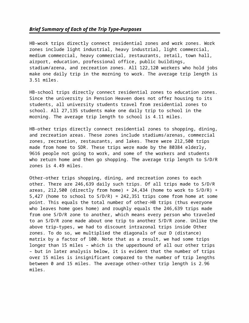
Brief Summary of Each of the Trip Type-Purposes

HB-work trips directly connect residential zones and work zones. Work zones include light industrial, heavy industrial, light commercial, medium commercial, heavy commercial, restaurants, retail, town hall, airport, education, professional office, public buildings, stadium/arena, and recreation zones. All 122,120 workers who hold jobs make one daily trip in the morning to work. The average trip length is 3.51 miles.

HB-school trips directly connect residential zones to education zones. Since the university in Pension Heaven does not offer housing to its students, all university students travel from residential zones to school. All 27,135 students make one daily trip to school in the morning. The average trip length to school is 4.11 miles.

HB-other trips directly connect residential zones to shopping, dining, and recreation areas. These zones include stadiums/arenas, commercial zones, recreation, restaurants, and lakes. There were 212,500 trips made from home to SDR. These trips were made by the 80384 elderly, 9616 people not going to work, and some of the workers and students who return home and then go shopping. The average trip length to S/D/R zones is 4.49 miles.

Other-other trips shopping, dining, and recreation zones to each other. There are 246,639 daily such trips. Of all trips made to S/D/R areas, 212,500 (directly from home) + 24,434 (home to work to S/D/R) + 5,427 (home to school to S/D/R) = 242,351 trips come from home at some point. This equals the total number of other-HB trips (thus everyone who leaves home goes home) and roughly equals the 246,639 trips made from one S/D/R zone to another, which means every person who traveled to an S/D/R zone made about one trip to another S/D/R zone. Unlike the above trip-types, we had to discount intrazonal trips inside Other zones. To do so, we multiplied the diagonals of our D (distance) matrix by a factor of 100. Note that as a result, we had some trips longer than 15 miles – which is the upperbound of all our other trips – but in later analysis below, it is evident that the number of trips over 15 miles is insignificant compared to the number of trip lengths between 0 and 15 miles. The average other-other trip length is 2.96 miles.

Demand for Transportation: Trip Distribution

Overview of Trip Array Generation2

The trip distribution for Pension City is based on the Gravity Model. This model is in fact similar to Newton’s theory of gravity; it assumes that trips produced at an origin and attracted to a destination are directly proportional to the total trip productions at the origin and the total attractions at the destination. The calibrating term—in our case, the “friction factor” (F) – represents the reluctance or impedance of persons to make trips of various duration or distances. The general friction factor indicates that as travel times increase, travelers are increasingly less likely to make trips of such lengths. Calibration of the gravity model involves adjusting the friction factor. The other adjustment factor associated with the Gravity Model is the socioeconomic adjustment factor (K), but in our case we have this factor equal to 1 and therefore has no impact.

A crucial consideration in following the Gravity Model is the “balancing” production and attraction vectors. This means that the sum of the productions must equal the sum of the attractions for each trip-type. In the trip distribution for Pension Heaven, the Gravity Model is as follows:

T ij=A jF ijK ij

∑all zones

AxF ijK ixx Pi

Where:T ij = trips produced in zone i and attracted to jPi = total trip production in zone iA j = total trip attraction to zone jF ij = friction factor; a calibration term for spatial separation between zones ijK ij = a socioeconomic adjustment factor for interchange ij = 1i = origin zonen = number of zones

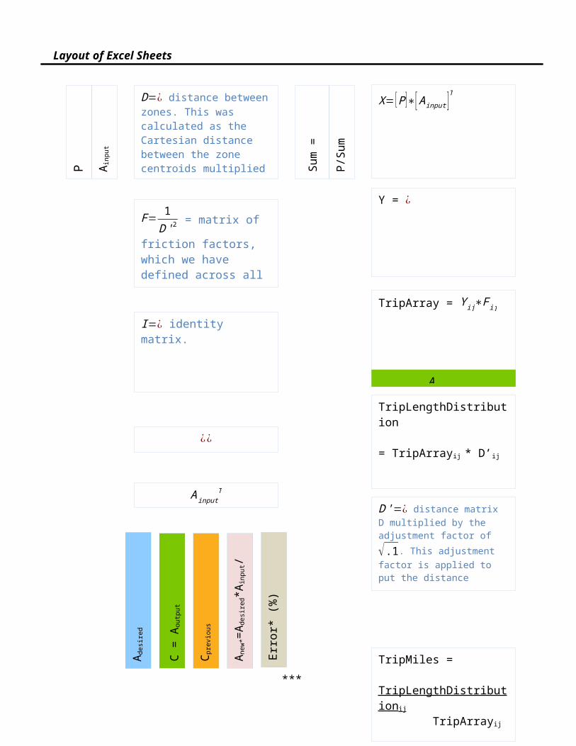
We used this above Gravity Model to generate the TripArray matrices for all nine types of trips between Home, Work, School, and Other. Our excel sheets are consistent in their calculations, as laid out below:

2 http://www.princeton.edu/~alaink/Orf467F12/The%20Gravity%20Model.pdf

Layout of Excel Sheets

***

P A inp

ut

D=¿ distance between zones. This was calculated as the Cartesian distance between the zone centroids multiplied by 1.2 which is a factor accepted as a good estimate of the circuitry.

X=[P ]∗[ Ainput ]T

Sum

=

P/Su

m

Y = ¿F= 1D' 2

= matrix of friction

factors, which we have defined across all trip purposes as the inverse of the distance squared.

I=¿ identity matrix. TripArray = Y ij∗F ij

Aoutput

TripLengthDistribution

= TripArrayij * D’ij

D '=¿ distance matrix D multiplied by the adjustment factor of √ .1. This adjustment factor is applied to put the distance between cells in terms of miles (since the centroids are in an improper coordinate system).

TripMiles =

TripLengthDistributionij TripArrayij

¿¿

AinputT

A des

ired

C =

A out

put

C pre

viou

s

A new

*=A d

esire

d*A i

nput

/Cpr

evio

us

Erro

r* (%

)

blue = constant matrix

**To compute the iterations dictated by the Gravity Model, we used the colored vectors above.

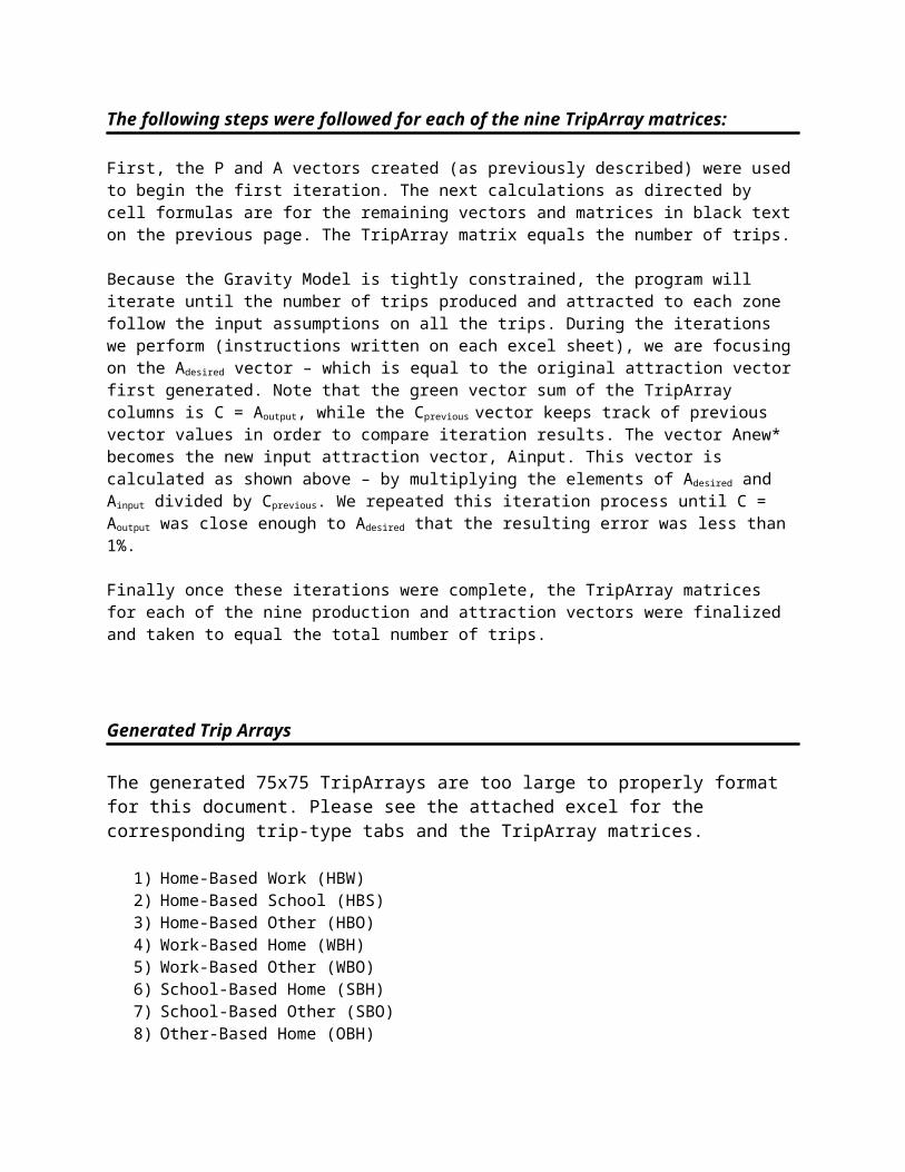
The following steps were followed for each of the nine TripArray matrices:

First, the P and A vectors created (as previously described) were used to begin the first iteration. The next calculations as directed by cell formulas are for the remaining vectors and matrices in black text on the previous page. The TripArray matrix equals the number of trips.

Because the Gravity Model is tightly constrained, the program will iterate until the number of trips produced and attracted to each zone follow the input assumptions on all the trips. During the iterations we perform (instructions written on each excel sheet), we are focusing on the Adesired vector – which is equal to the original attraction vector first generated. Note that the green vector sum of the TripArray columns is C = Aoutput, while the Cprevious vector keeps track of previous vector values in order to compare iteration results. The vector Anew* becomes the new input attraction vector, Ainput. This vector is calculated as shown above – by multiplying the elements of Adesired and Ainput divided by Cprevious. We repeated this iteration process until C = Aoutput was close enough to Adesired that the resulting error was less than 1%.

Finally once these iterations were complete, the TripArray matrices for each of the nine production and attraction vectors were finalized and taken to equal the total number of trips.

Generated Trip Arrays

The generated 75x75 TripArrays are too large to properly format for this document. Please see the attached excel for the corresponding trip-type tabs and the TripArray matrices.

1) Home-Based Work (HBW)2) Home-Based School (HBS)3) Home-Based Other (HBO)4) Work-Based Home (WBH)5) Work-Based Other (WBO)6) School-Based Home (SBH)7) School-Based Other (SBO)8) Other-Based Home (OBH)9) Other-Based Other (OBO)

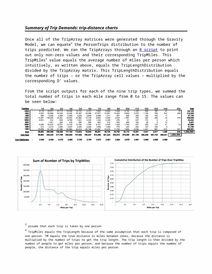
Summary of Trip Demands: trip-distance charts

Once all of the TripArray matrices were generated through the Gravity Model, we can equate3 the PersonTrips distribution to the number of trips predicted. We ran the TripArrays through an R script to print out only non-zero values and their corresponding TripMiles. This TripMiles4 value equals the average number of miles per person which intuitively, as written above, equals the TripLengthDistribution divided by the TripArray matrix. This TripLengthDistribution equals the number of trips – or the TripArray cell values – multiplied by the corresponding D’ values.

From the script outputs for each of the nine trip types, we summed the total number of trips in each mile range from 0 to 15. The values can be seen below:

3 assume that each trip is taken by one person

4 TripMiles equals the TripLength because of the same assumption that each trip is composed of one person. TM equals the true distance in

miles between zones, because the distance is multiplied by the number of trips to get the trip length. The trip length is then divided by the number of people to get miles per person, and because the number of trips equals the number of people, the distance of the trip equals miles per person

Below are the nine TripLength distributions for the number of trips vs. trip miles:

As expected, the shape of the Home-Based Work distribution is the same as the return trip home. The two graphs differ in their Number of Trips – this makes sense, because only 80% of the HBW trips become WBH trips. This distribution jumps quickly at low Trip Miles values, and quickly decreases as the Trip Miles increases. This distribution seems logical, as often people choose their residence based on proximity to place of work. We can see a steep s-curve in the cumulative distribution, and the right tail is also is what we expect for this trip distribution.

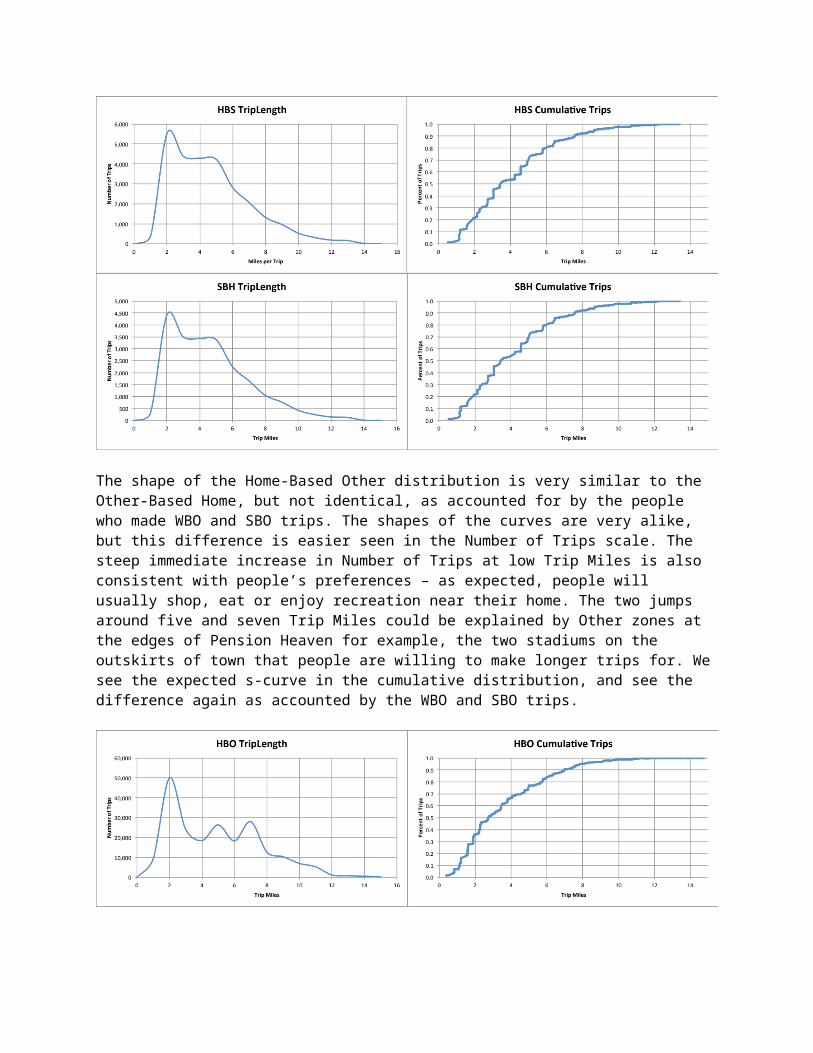
Also as expected, the shape of the Home-Based School distribution is the same as the return trip home. Just as above, the two graphs differ in their Number of Trips – which also makes sense, because only 80% of the HBS trips become SBH trips. The steep increase in number of trips at low Trip Miles makes sense, as children attend the public school in their designated district. The tail of this distribution is less severe than the above distribution for the work-commute—this, and the temporary flat line in the graph could be explained by the distances people are willing to travel to take their children to the private day school. In the cumulative distribution graph, we can again see an s-curve and a right tail – not as extreme as the HBW right tail, which is accounted for by the above reasons.

The shape of the Home-Based Other distribution is very similar to the Other-Based Home, but not identical, as accounted for by the people who made WBO and SBO trips. The shapes of the curves are very alike, but this difference is easier seen in the Number of Trips scale. The steep immediate increase in Number of Trips at low Trip Miles is also consistent with people’s preferences – as expected, people will usually shop, eat or enjoy recreation near their home. The two jumps around five and seven Trip Miles could be explained by Other zones at the edges of Pension Heaven for example, the two stadiums on the outskirts of town that people are willing to make longer trips for. We see the expected s-curve in the cumulative distribution, and see the difference again as accounted by the WBO and SBO trips.

The WBO distribution has the two most drastic jumps in Number of Trips. We expect every graph to have the first significant, steep peak in the low Trip Miles values, but the second peek around four Trip Miles is after a significant trough. This can logically be explained; those leaving work for Other zones (ie a restaurant or commercial zone) would most likely prefer a zone close to their place of business – purely out of convenience. The second peak could be explained by trips that workers have to make – in other words, the zone is not selected based on proximity but on the specific, perhaps necessary, destination. These two peaks are also seen in the drastic jumps of the s-curve in the cumulative distribution graph.

The SBO distribution is unique in that after the first expected peak at low Trip Miles, the Number of Trips increases. This could be explained by what types of Other zones are congregated around the six different schools. For example, the school in zone 74 is far from the restaurant and retail zones as compared to the other five schools. The cumulative distribution is still an s-curve, but is not as steep as the previous charts. This is expected from the TripLength graph’s dispersion of trips.

This OBO distribution graph is essentially unimodel, with a large peak around two Trip Miles. This is not out of place because the layout of Pension Heaven is such that most of the Other zones are clustered around each other, as are the Residential and Work zones. Intrazonal trips inside Other zones were discounted by multiplying diagonals of the D (distance) matrix by a factor of 100. Although some trips were longer than 15 miles – the upperbound of all our other trip-types – the graphs below demonstrate that the number of trips over 15 miles is insignificant compare to those between 0 and 15 miles. The cumulative trips distribution only appears to be the steepest s-curve, but that is only a result of the scaling; when we take the x-values between 0 and 15, the s-curve is more similar to previous distributions.

*note that for comparison purposes in the tables below, we included any OBO trips over 15 miles long in the 15 TripMiles.

TripLength Distribution Analysis

When we transform each trip-type into percentage of trips across the different trip lengths, we can better compare the different distributions. The shapes are relatively similar among all the series with the slight exception of the OBO and WBO trips. The first peaks of OBO and WBO line are both at low miles and account for the largest percent of their trip-type counts, which seems appropriate. People traveling from work-to-other and other-to-other and more inclined to go to an Other zone in close proximity; both because of preference and also the clustering of Other zones around Work zones and different Other zones.

In the cumulative distribution graph below, we also see that the OBO and WBO curves are slightly different from the other distributions, in their high occurrence of trips in the low mile category.

Appendix

R Script used to cycle out zeros in TripArray matrices for each of the nine different trip types

#HBW #HBWTripArray.csv is a file containing only the 75x75 TripArray matrix HBWTripArray<-read.csv("HBWTripArray.csv",header=FALSE);HBWTripMiles<-read.csv("HBWTripMiles.csv",header=FALSE);

#finding indices of non-zero valuesX<-which(HBWTripArray!=0,arr.ind=T);

#creating new matrix of non-zero [TripMiles, Trips]HBW_PTMvsT<-matrix(0,length(X[,1]),2)HBW_PTMvsT[,1]<-HBWTripMiles[X];HBW_PTMvsT[,2]<-HBWTripArray[X];HBW_PTMvsT<-round(HBW_PTMvsT,digits=4);

write.matrix(HBW_PTMvsT,file="HBW",sep=",")

The above script was used for all nine trip-types