Ex. No: TOKEN BUS PROTOCOL

Aim: To create the scenario and study the performance of token BUS LAN protocol through

simulation and using trainer kit

Apparatus Required:-LAN Trainer KitSimulation software & PC

Theory:-IEE standard 8024 describes a LAN called a token bus physically, the token bus is a

linear(or) three shaped cables on to which the simulation are attached logically the stations are organized into rings, with each station knowing the address of the station to its left and right when the logical ring is initialized the highest numbered station may send the first frame. After it is done it passes permission to its immediate neighbors a special context.Experimental Procedure:

The physical connection was shown in fig.Step 1:-

Connect RS-232 LANs cables from PC to converter codes. Select RS-485 LAN BUS cable to the converter card

Step 2:- Connect the other ends of the bus to connect Ib on the ended nodes. Run the LAN trains software

Step 3:-Choose the serial port settings as shown in fig. below by selecting a serial communication port parameter on the embedded node.

Step 4:-Connect all the three boards and a PC interface to the respective power

supply following message. “LAN Tr node”.The following message appears on the LCD, “waiting for SCF”. SCF

means “Start us check Frame”Step 5:-

Inter electro technologies- network concept trainer (LAN) service. Start LAN demo serial port setting help exit. The following “Addressing nodes and address” window opens.

Figure 1:-Addressing nodes and address

Select number of nodes : 3 Help

Address of network monitor

Node address cancel

Select node address:1

Select node address:3 next

Select node address:4

Step 6:- Specify the parameter node address it you connected three address select the node

address. The address of network monitor is taken as 2 by default which can not be changedObservation:-

The network monitor transmits 01c2# to node1 where,

SD DA Frame type© SA ED

0 is the start delineator1 is the destination addressc is the frame type2 is the source address#--> is the end delineator.

Figure 2:- The response received for frame

Status check frame Help

Send status check frame to : 1

Send status check frame to : 3 cancel

Send status check frame to : 4 back

Frame 02x1H02x3#02x1# Next

Experimental procedure:-

On clicking next in the screen 3 that is sending the status check frame to all the nodes and receiving the next frames will enter to send successor predecessor frames screen.

Status check frame Help

Send status check frame to : 1

Send status check frame to : 3 cancel

Send status check frame to : 4 back

Response received next

Click on next to enter into network monitor screen for network and local management.

Observation

SD DA Frame type©

Succ address

Pree addr

ED

Status check frame Help

Send status check frame to : 1

Send status check frame to : 3 cancel

Send status check frame to : 4 back

Response received 02H1#02H3#02H4# next

The acknowledgment to the transmitted frame like 02H1#,02H3#, 02H4# are received frame node 1,3, 4 respectively

The embedded node comes to the main menu after transmitting the acknowledgementMain menu on embedded system:-

1. status2. transmit message3. Display message4. Disconnects

To check the staus of the embedded node key ‘1’ is pressed To transmit the message of the embedded node key ‘2’ is pressed To disconnect of the embedded node key ‘4’ is pressed,

Result:Thus the performances of token bus protocol were studied through simulation.

Ex. No: TOKEN RING PROTOCOL

Aim: To create the scenario and study the performance of token ring LAN protocol through simulation

and using trainer kit

Apparatus Required:-LAN Trainer KitSimulation softwarePC

Theory:-Token ring allows each station to send frame per turn the mechanism that to-ordinate

a simple place folder frame that is passed from station to station around the ring. Whenever the network is uncoupled it circulates a sample three byte token. It keeps the token and sets a bit inside it. NIC as a reminder that it has done said to one data frame. This data frame proceeds around the ring. The sender receivers the frame and recognize itself in the source address bits. It they are set it knows that frames were received the sender and release the token back to the ring.

Experimental Procedure:

Step 1:-Turn on the embedded node. Connect all the tree nodes and PC to the respective power supplies. Switch on the power supply to all the nodes

Step 2:- After the embedded node completes the self test on the peripheral phase, Enter the target address accept address‘s’ because this address is embedded to network motion.

Example:- user can enter address’5’ ‘2’’4’ on the embedded nodes.Address nodes to the token ring objective

To add embedded nodes to the token ring network by transmitting duplicate check frame.Experimental Procedure:

Step 3:- Click on “start token ring” on the network monitor frames. Click the initialized ring button to transmit DCF to the nodes

Step 4:-

On the embedded node one can a bserved the following message received DCF. Once all the nodes receive the DCF to acknowledgement can be seen on the screen

0 is the staring decimeter1is the access control fieldA is the Board casting treeU is the frame type DCFZ is the source address network monitor.

Transmit token frame:-Step 5:-

Token will start rotating through the entire nodes infinitely token an LED glass on the real switch.

Step 6:- One complete plate rotation of the cycle (or) when the network monitor receiver the token bus.

Step 7:- Click the next button to go the next screen to check the status of the embedded node ‘1’ on the embedded node screen.

If the node ‘1’ it shows1 staus2 transmit message3 display4 disconnect

Frame:- SD frame type

This is control frame generated by the network monitor end and passed in a ring. The nodes after receives the frame from the previous node.

It check any data on control frame to the transmit otherwise. Release the token to next station is the ring frame format

0 start of frame1-Access contro fieldq- end decimeter

there are two types of communication1. point to point

To transmit data from one point to another2. Broad cast

To Broad cast data from one node to all node

Result:

Thus the performance of token ring protocol was studied through simulation.

Ex. No: STOP & WAIT ARQ PROTOCOL

Aim: To conduct an experiment to demonstrate the working of the basic stop and wait protocol.

Apparatus Required:-Simulation softwarePC

Theory:-DataLink Layer:-The data link layer transforms the physical layer is a raw transmission facility to a reliable link and is responsible for node to node delivery

Framing Physical addressing Flow control Error control Access control

Stop and wait (Flow control)In a stop and wait method of flow control the sender waits for an acknowledgement

has been received is the next frame send. This process of alternatively sending and waiting repeats until the sender transmits an end to transmission frame. The advantage of stop and wait protocol is simplify and disadvantage is inefficiency.

Stop and wait AR2(Error control)AR2 means automatic request is a form of stop and wait flow control extended to

conclude retransmission of data in case of lost (or) damaged frames.

When a frame is discovered by the receiver to contain on error it returns a NAK frame and the sender retransmit the past frame.

Normal operation:-In the normal operation the sender sends frame 1 and waits to receive Ack, when

Ack1 is recived it sends frame1 and the wait ti avk 0 and so on. The ack must be retained before the timer expeies.

Lost (or) Damage:-A lost frame is handled in the same way by the receiver, when the receiver a damaged

frame, it discards.

Lost Ack:-A lost (or) damaged ack is handled in the same way by the sender, the waiting

sender doesn’t know if frame1 has been received when the timer for frame1 expires the sender retransmit frame1.

Delayed Ack:-An Ack can be delay at the receiver. The delay of ack it is received after the timer

frame 0 has already expired. The sender has already transmitted a copy of frame0. Therefore it discards the duplicate frame the stop and wait mechanisms id unidirectional We have this the two parties have two separate channels. In this case, the data frame frame has made it is the receiver transmit.

Experimental Procedure:

Step 1:- Power up the systems.

Step 2:-change to the directory where CD Contents are copied (example: cd NLSBackup / layers /Phy_lyr)

Step 3:- Execute the file “./runmod main” (dot slash runmod main)

Step 4:- From main menu Choose Layers _ Data Link Layer _ Stop and Wait Protocol.

Step 5:-After choosing the stop and wait protocol, Click on “Let’s Begin” button on both systems the following screen1 will be displayed.

Step 6:- Choose the number of frames to transmit in first node.

Step 7:-Choose the Start char, End char and Pad char of frames in both the systems, by default other than data and these three characters should be same in both the systems.

Step 8:- Send maximum of 8 bytes of data and click on send.

Step 9:- The receiving section will receive the frame as shown in Screen2.

Step 10 :- Click on Send ACK on the second node.

Step 11:-The sending section (first node) will receive the acknowledgement as Shown in

Screen3.

Observation:

The following observations can be made with the above experiment:1. With the RS-232 connection, frame can be transmitted between systems and

simple build up of protocol process is established.2. The working of the stop and wait protocol is understood in this experiment.3. Start, end, pad characters must be same on both ends to achieve error free

communication.4. The data in data link layer is in the form of frames and hence the start and end

characters are required to mark the start and end of a frame. Since the min no of data bytes in a frame is also fixed, the padding characters will be filled into the frame, of user entered data is less than the frame size.

Output:-

Result:Thus the experiment to demonstrate the working of basic stop & wait protocol was

conducted.

Ex. No: GO BACK - N & SELECTIVE REPEAT PROTOCOL

Aim: To conduct an experiment to demonstrate the working of the sliding window protocol.

Apparatus Required:-Simulation softwarePCRS232 cable

Theory:-In sliding window technique, there ere 2 types

Go back to N protocol Selective & repeat protocol

The feature are add to basic flow control mechanism generally sliding window means sender can transmit several frames before needing an Ack. In this sliding window Go back to N ARQ method if one frame is lost (or) damaged all frames send. Since the last frame acknowledged are retransmitted. So consider if frame 0 to 4 have been transmitted before a NAK is received for frame 2 As soon as received discovers an error its stop accepting subsequently the frames until the damaged frame has been replaced.

Correctly data 2 arrives damaged and so is discarded as are data 3 and data 4, whether or not the have arrived infect data 1 and data1 which where received before the damaged frame have already accepted a fault indicated to the sender by the NAK 1 frame.

Selective Repeat ARQ:

In selective repeat, some specific operation was performed.Lost frame:

Frame 0 & frame 1 are accepted because they are in the range specification by this receivers window when frame3 is received sends a NACK 2 to show that frame 2 has not been received then the sender receiver NAK2 its sends only frame 2 which is then accepted.Lost and delayed Ack’s and Nak’s

There is a possibility for lost and delayed Ack’s and NAK’s for that the sender sets a timer for each frame sent

Experimental Procedure:

Step 1:- Power up the systems.

Step 2:- Change to the directory where CD Contents are copied (example: cd NLSBackup / layers /Phy_lyr)

Step 3:- Execute the file “./runmod main” (dot slash runmod main)Step 4:- Choose Layers _ Data Link Layer _ Sliding Window Protocol.

Step 5:- After choosing Sliding Window Protocol, Click on “Let’s Begin” button on both the system screen1 will be displayed.

Step 6:-Enter the start, end and pad characters of frame in both sections, by default other than data.

Step7:- Enter a maximum of 8 bytes of data on the first system and click on send.Step 8:-

The receiving area will receive the frame.Step 9:-

The receiving end receives all 7 frames.Step:- 10

Send sequence number and click on RR N button in the receiving section, to get more than 7 frames; the sending end will receive the RR N sequence number as shown in Screen2.

Step 11:- After receiving RR N sequence number sending end will be transmitted the remaining frames as shown in Screen3.

Observation:The following observations can be made with the above experiment:

With the RS-232 connection, frame can be transmitted between systems and simple build up of protocol process is established.

Start, end, pad characters must be same on both ends to achieve error free communication.

The working of the sliding window protocol is understood in this experiment for link utilization and acknowledgement scheme with reference to Stop and Wait Protocol.

Output:-

Go back N:-

In stop and wait ARQ at any time for a sender there is only one format that is send and waiting to be Ack. To improve the efficiency multiple frames should be in transmission while waiting for a Acks. In Go back N ack2 we can send up to 10 frame, before ack we keep a copy of these formats frames until the acknowledgement.

Damaged (or) lost framesThere frame 2 is lost note that when the receiver receives frames 3 it is discarded

because the receiver is expecting frame 2 expires at the sender sends frame 2 & 3.

Experimental procedure:

Step 1:- Power up the systems.

Step 2:-Change to the directory where CD Contents are copied (example: cd NLSBackup / layers /Phy_lyr)

Step 3:- Execute the file “./runmod main” (dot slash runmod main)

Step 4:- Choose Layers _ Data link layer _ Sliding window.

Step 5:-Choose Program _ go-back-n form the menu.

Step 6:-After choosing the go-back-n protocol, Click on “Let’s Begin” button on both systems the following screen1 will be displayed.

Step 7:-Choose number of frames to transmit.

Step 8:- Choose start, end and pad characters, by default other the data.

Step 9:-Enter a maximum of 8 bytes of data on the first system, click on the SEND button.

Step 10:- If user wants to include error click on ERROR button, include the error in the frame then click on the SEND button.

Step 11:-The receiving section (second node) receives 7 frames.

Step 12:-Then receiver enters sequence number and click on the REJ button, the sending end will receive the warning as shown in Screen2.

Step 13:-The frames will be retransmitted from specified sequence number to all frames as shown in Screen3.

Observation:

The following observations can be made with the above experiment: With the RS-232 connection, data can be transmitted between systems. The port parameters are enhanced to handle more complicated, detailed associated

with the port. Start, end, pad characters must be same on both ends to achieve error free

communication. The working of sliding window- Go- Back- N protocol is understood in this

experiment. In this mechanism the data will retransmitted from the frame for which the REJ-N frame is received.

Result:- Thus the performance of sliding Window protocol was demonstrated and output was verified.

Ex. No: SHORTEST PATH ALGORITHMS

Aim:To conduct an experiment to demonstrate the working of the shortest path algorithm.

Apparatus Required:-Simulation software4 no. of PC RS232 cable

Theory:- The idea of shortest path routing is to build in graphs of the submit with each node

representing is router and each graph represents a communication time. To choose a route between a given pair of returns the algorithm just finds the shortest path between them on the graph.

The concepts of a shortest path deserve some explanation an way of meaning path length in the number of hops. Another metric in the geographic distance longer than ABE.

Initially no paths are labeled with infinity. As the algorithm processed and path are found the labels may rejecting better paths.

A label may be either tentative initially all labels are tentative when is discovered that a label represent.

The reason for searching backward in that each node is labeled with its predecessor rather. The cost of the arc from network to router is always Zero.

Shortest Path Tree The dijikstras algorithm follows four steps to discover what is called the shortest path tree for

each router. The algorithm begins to build the tree by identifying its root, the root at each routers tree is

the router it self Nodes and reached from that roots nodes and arcs are temporary at this step. The last two steps are represented until every node in the network has become a permanent

part of the tree. The steps of the dijikstras algorithm applied by node of our sample internets. The cost

number next to each node represent.

Routing Table: Each router now uses the shortest path tree to construct its routing table each router use the

same algorithm and the same link state data base to calculate its own shortest path tree and routing table these are different for each router.

For each router two common modes are used to calculate the shortest path between two routers distance vector routing and link state routing so, the path way with the lowest cost is considered the best.

As long as the cost of each link is known a router can find several routing algorithm exists for making these calculations.

The most popular are distance vector routing and link state routing. In this the cost should be provided in the way.

Procedure:-

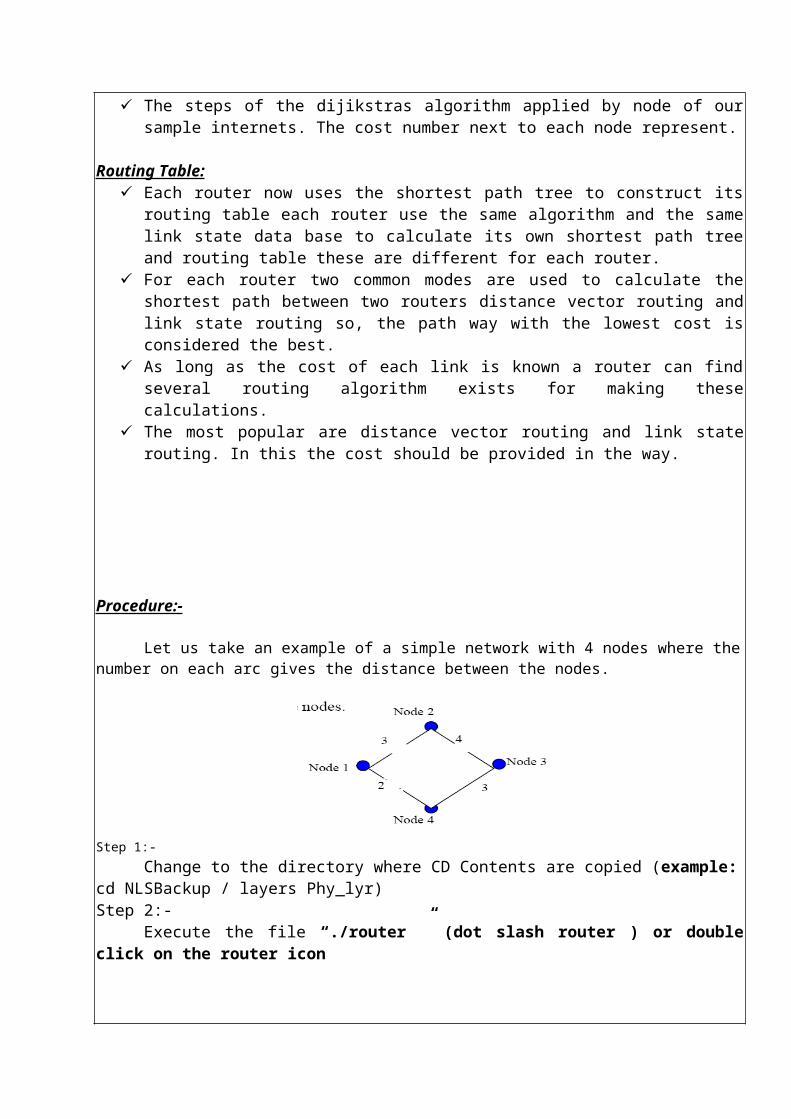
Let us take an example of a simple network with 4 nodes where the number on each arc gives the distance between the nodes.

Step 1:-

Change to the directory where CD Contents are copied (example: cd NLSBackup / layers Phy_lyr)Step 2:-

Execute the file “./router ” (dot slash router ) or double click on the router icon

Select Shortest Path Algorithm menu option from the main menu

After selecting Shortest Path, the shortest path Window opens and here we need to enter the values as explained below to configure it

Enter the own node (The node number assigned to this Pc, On Pc1 the own node would be 1 and on 2 it would be 2 and so on…).

Enter the no of nodes in the network. In the example that we have taken, there are 4 nodes in the network.

Now we need to enter the distances between nodes in the distance matrix as shown in the figure below. In the example network the distance between node 1 and node 2 is 3 and node 1 and node 4 is 2… similarly we fill in the distances between nodes in the matrix as shown in the figure below.

Once the above information is entered check the info and click on ok button. The same steps need to be followed on all the 4 pc’s (node 1, 2, 3, 4). The only

difference being the value in ‘own node’ field.

Step 3:-After clicking OK, in the router window, the Messenger Window will open, In this window to see the shortest distance click on the Show Table Button as shown in the below figure

After clicking on the show table the result of shortest distance is displayed as shown in figure

1 = 0 (This represents Path from Node1 to Node 1 and the distance is 0)12 = 3 (This represents Path from Node 1 to Node 2 and the distance is 3)143 = 5 (This represents Path from node 1 to Node 3 shortest path is through Node 4 and the distance is 5..14 = 2 (This represents path from Node 1 to Node 4 and the distance is 2).Once the above process is over, we can send the message from node to node .For example suppose if you want to send a message from Node 1 to Node 2. Enter the Destination Node number in the Destination block and the message in the text area at the bottom of the window. Then click send to send the message as shown in below Figure.

Once all the nodes are configured messages can be sent from any Node to any other Node in the network. We can see that the message will take the path calculated by shortest path algorithm. If a message is sent form node 1 to node 3 then the message is first received by node 4 and then node 4 forwards the message to node 3.

Result:-

Thus the working of shortest path routing was conducted and output was verified.

Ex. No: LINK STATE ROUTING

Aim: To conduct an experiment to demonstrate the working of the link state routing algorithm.

Apparatus Required:-Simulation software4 no. of PC Telnet connection

Theory:- The keys to understanding link state routing are different from those in distance vector

routing. In link state routing each router shares its knowledge of its neighbourhood with every other router in the network.

Information sharing when there is a change. In link state routing each router shares its knowledge of its neighbourhood will all router in the internet work

Packet cost:-

Both distance vector and link state routing are lowest cost algorithm. In distance vector routing cost refers tp help count in link state routing cost is a weighted value based on a varieties of factors such as security levels.

State at the link, the cost from router A to N. therefore might be different from the cost from A to 23. cost is applied only by routers and not by another stations on a network member the link from one router to the next.

Cost is applied as a packet leaves the router than as it enters most of network are broad cast network when packet is in the network every station including the router can pickup.

There fore we cannot when it goes from a network to a routerLink state Packet

When a router floods the network with information about its neighbour hood it is said to be advertising the basic of this advertising is a short packet called a link state packet.

An LSP usually contains four field. The ID of the advertiser the ID of the destination network the cost of the ID of the neighbour router.

Initialization Imagine that all routers in our sample internet work come up at the same time each router

sends a greeting packet to its neighbour to find out the state of each link. In the prepare, an LSP based on the results of these greetings and floods the network with it.

The same steps are performed by every router in the network as each comes Up.Link state Data Base

Every router receives every LSP and puts the information in to a link state data base. Because every router receives the same LSPs every router builds the same database.

It stores this data base on its disks must be stored for fast updating.

Procedure:-

Let us take an example of a simple network with 4 nodes.

Step 1:- Select the Link State routing algorithm from the menu or by selecting the shortcut icon

Step 2:-After selecting on the Link State algorithm, the Link State Window will open and we need to enter the values as explained below to configure it.

Enter the own node (The node number assigned to this Pc, On Pc1 the own node would be 1 and on 2 it would be 2 and so on…).

Enter the no of nodes in the network. In the example that we have taken, there are 4 nodes in the network.

Also we need to select the neighboring nodes .For the above example Node 1 is connected to Node 2 so we tick on that particular Node.

Step 3:- After configuring and clicking on the O.K button the messenger window will open. Click on

the Show table you can see the path to all other nodes is unknown initially.Once the other nodes come up the path will be obtained automatically by sending hello

packets and neighbor info to all other nodes. Here this algorithm is different from distance vector.In distance vector the neighbour info is sent to only other neighbours whereas in link state routing neighbour info is sent to all other nodes

Step 4:- Similarly you configure for other systems by clicking the Executable Routers with the same

procedure as explained above.

Once all the nodes come up, they will exchange their neighbor information with all other nodes and calculate the shortest to all the nodes in the network. The shortest path from a given node to all other network can be seen by clicking on the show table button on the messenger window. The below figure explains the passing message from Node 1 to Node 4. The message from node 1 to node 4 will have to pass through node 2 as the path from 1 to 4 is 1-2-4 as shown in the below figure.

When the message is sent to node 4, the packet will first be sent to the node is the path column. In this case the packet is first sent to node 2, which will then forward the packet to node 4.

Result:-

Thus the working of link state routing was constructed and the output was verified

Ex. No: DISTANCE VECTOR ROUTING

Aim: To conduct an experiment to demonstrate the working of the Distance vector routing algorithm.

Apparatus Required:-Simulation software4 no. of PC Telnet connection

Theory:-In distance vector routing each router periodically shares its knowledge about the entire

network its neighbors’. The tree keys to understanding how this algorithm work are follows as. Knowledge about the whole network Routing only to neighbours Information sharing at regular intervals

Sharing information:- To understand how distance vector routing works, examine the interest shown. The

inside each close is that LAN s network. These LANs can be any type the LAN s are connected bores labeled A,B,C,D,E,F. A

router sends its knowledge to its neighbour the neighbour add Enentuallu every states knows about every other router in the internet work.

Routing Table:- Now lets examine how each router sets its initial knowledge of the interval worn is

sparse. All number of LANs it also knows the ID of each station. A routing table was columns for at least three and the next router is the router to

which a packet must be delivered to which a packet must be delivered on its way to a particular destination.

Updating the table:- When A receives a routing table from B it uses the information to update its own table. It

says to itself B has sent a table get to network ss &14. Router ‘\A--------finds which even version shows the lower lost. This selection process is the reason for the cost column the lost the save reservation.

Every router receives information from neighbour and update its routing table.Udating Algorithm:-

The updating algorithm requires that the router first add one hop to hop count field for each advertised router. The router should then apply the following rules to each advertising destination is in the routing table.

If a next hop field it the same. The router should replace entry in the table because the near information invalidated the old.

If the next hop field is not the same. If the advertised hop count is smaller than the one in the table, the router should replace the entry in the table with the network.

Procedure:-Let us take an example of a simple network with 5 nodes.

We will take the above example distance vector entering the values. The values need to beentered on all the pc’s that is to be used as nodes. Here we are taking the number of hops as the metrics for calculating best path to the destination node.

1. Select the Distance vector routing algorithm from the menu or click on the on the shortcut for distance vector.

2. After selecting the Distance Vector algorithm, the Distance Vector Window will open and we need to enter the values as explained below to configure it.

Enter the own node (The node number assigned to this Pc, On Pc1 the own node would be 1 and on 2 it would be 2 and so on…).

Enter the no of nodes in the network. In the example that we have taken, there are 5 nodes in the network.

Also we need to select the neighboring nodes .For the above example Node 1 is connected to Node 2 and Node 5 so we tick on that particular Nodes.

Step 3:- After configuring and clicking on the O.K button the messenger window will open. Click on

the Show table you can see the path to all other nodes is unknown initially. Once the other nodes come up the path will be obtained automatically by sending hello packets and neighbor info to other neighbors

4. Similarly you configure for other systems by providing correct information as explained above

Similarly configure nodes 4 and 5.

Once all the nodes come up, they will exchange their neighbor information with their neighbors and calculate the next hop for the packet as well as the number of hops to destination. The path with least number of hops is selected.

In this algorithm also we can understand the algorithm and the path taken by packet by sending messages from one node to another. Below figure explains the passing message from Node 1 to Node 3 through Node 2, since we are explaining the example from above Figure it will choose less No of hops to travel from node 1 to node 3 as shown below

When the message is sent to node 3, the packet will first be sent to the node is the path column. In this case the packet is first sent to node 2, which will then forward the packet to node 3

Result:-

Thus the working of distance vector routing was constructed and the output was verified.

Ex. No: STUDY OF NETWORK SIMULATOR Aim :

To Study the Network simulator (NS)Introduction :

NS (from Network Simulator) is a name for series of discrete event network simulators, specifically ns-1, ns-2 and ns-3. All of them are discrete-event computer network simulators, primarily used in research and teaching. ns-3 is free software, publicly available under the GNU GPLv2 license for research, development, and use.The goal of the ns-3 project is to create an open simulation environment for computer networking research that will be preferred inside the research community:

It should be aligned with the simulation needs of modern networking research.

It should encourage community contribution, peer review, and validation of the software.

Since the process of creation of a network simulator that contains a sufficient number of high-quality validated, tested and actively maintained models requires a lot of work, ns-3 project spreads this workload over a large community of users and developers.History:

ns-1The first version of ns, known as ns-1, was developed at Lawrence Berkeley National Laboratory (LBNL) in the 1995-97 timeframe by Steve McCanne, Sally Floyd, Kevin Fall, and other contributors. This was known as the LBNL Network Simulator, and derived from an earlier simulator known as REAL by S. Keshav. The core of the simulator was written in C++, with Tcl-based scripting of simulation scenarios.ns-2Ns began as a variant of the REAL network simulator in 1989 and has evolved substantially over the past few years. In 1995 ns development was supported by DARPA through the VINT project at LBL, Xerox PARC, UCB, and USC/ISI. Currently ns development is support through DARPA with SAMAN and through NSF with CONSER, both in collaboration with other researchers including ACIRI. Ns has always included substantial contributions from other researchers, including wireless code from the UCB Daedelus and CMU Monarch projects and Sun Microsystems. For documentation on recent changes, see the version 2 change log.ns-3A team led by Tom Henderson, George Riley, Sally Floyd, and Sumit Roy, applied for and received funding from the U.S. National Science Foundation (NSF) to build a replacement for ns-2, called ns-3. This team collaborated with the Planete project of INRIA at Sophia Antipolis, with Mathieu Lacage as the software lead, and formed a new open source project.

In the process of developing ns-3, it was decided to completely abandon backward-compatibility with ns-2. The new simulator would be written from scratch, using the C++ programming language. Development of ns-3 began in July 2006. A framework for generating Python bindings (pybindgen) and use of the Waf build system were contributed by Gustavo Carneiro.

The first release, ns-3.1 was made in June 2008, and afterwards the project continued making quarterly software releases, and more recently has moved to three releases per year. ns-3 made its twenty first release (ns-3.21) in September 2014.

Current status of the three versions is:

ns-1 is no longer developed nor maintained,

ns-2 is not actively maintained,

ns-3 is actively developed (but not compatible for work done on ns-2).

Installing NS2:

There are two ways of using NS2: On Linux Operating System or on Windows Operating System.On Linux, after downloading NS2 follow these steps:

1. Copy ns-allinone-2.35.tar.gz file to your home directory.

2. Run terminal by pressing Ctrl+Alt+T .

3. Execute "tar -xzvf ns-allinone-2.35.tar.gz" command.

4. Execute "cd ns-allinone-2.35" command.

5. Execute "./install" command.

6. Execute "cd ns2.35" command.

7. Execute "./validate" command.

On Windows 7, first install Cygwin. After that go through the following steps:1. Copy ns-allinone-2.35.tar.gz file to cygwin folder

2. Execute "cd /" command.

3. Execute "tar -xzvf ns-allinone-2.35.tar.gz" command.

4. Execute "cd ns-allinone-2.35" command.

5. Execute "./install" command.

6. Execute "cd ns2.35" command.

7. Execute "./validate" command.

Design:

ns-3 is built using C++ and Python with scripting capability. The ns-3 library is wrapped by Python thanks to the pybindgen library which delegates the parsing of the ns-3 C++ headers to gccxml and pygccxml to automatically generate the corresponding C++ binding glue. These automatically-generated C++ files are finally compiled into the ns-3 Python module to allow users to interact with the C++ ns-3 models and core through Python scripts. The ns-3 simulator features an integrated attribute-based system to manage default and per-instance values for simulation parameters. All of the configurable default values for parameters are managed by this system, integrated with command-line argument processing, Doxygen documentation, and an XML-based and optional GTK-based configuration subsystem.The large majority of its users focuses on wireless simulations which involve models for Wi-Fi, WiMAX, or LTE for layers 1 and 2 and routing protocols such as OLSR and AODV.

Components :

ns-3 is split over couple dozen modules containing one or more models for real-world network devices and protocols.ns-3 has more recently integrated with related projects: The Direct Code Execution extensions allowing the use of C or C++-based applications and Linux kernel code in the simulations.

Simulation workflow:

The general process of creating a simulation can be divided into several steps:1. Topology definition: To ease the creation of basic facilities and define their

interrelationships, ns-3 has a system of containers and helpers that facilitates this process.

2. Model development: Models are added to simulation (for example, UDP, IPv4, point-to-point devices and links, applications); most of the time this is done using helpers.

3. Node and link configuration: models set their default values (for example, the size of packets sent by an application or MTU of a point-to-point link); most of the time this is done using the attribute system.

4. Execution: Simulation facilities generate events, data requested by the user is logged.

5. Performance analysis: After the simulation is finished and data is available as a time-stamped event trace. This data can then be statistically analysed with tools like R to draw conclusions.

6. Graphical Visualization: Raw or processed data collected in a simulation can be graphed using tools like Gnuplot, matplotlib or XGRAPH.

Result:Thus the Network Simulator was studied.