DEVELOPMENTS IN UPPER ATMOSPHERIC SCIENCEDURING THE IQSY

BY FRANCIS S. JOHNSON

SOUTHWEST CENTER FOR ADVANCED STUDIES, DALLAS, TEXAS

During the IQSY, there were of course many advances in the area of upper atmo-spheric science, and it would take a great deal of time and space to describe them alladequately. It is therefore necessary to arbitrarily select just a few of the advancesthat were, in my view, among the more important.

Neutral Upper Atmosphere.-The vertical structure of the atmosphere is in largedegree controlled by its temperature distribution, and the largest variations intemperature occur above 200-km altitude. This is illustrated in Figure 1, whichshows a typical temperature distribution up to 100 km, and three distributions athigher altitudes. The three distributions shown indicate near-extreme conditionsand an in-between, or average, situation. The range of variation can be seen to bevery great, far more than a factor of 2 at the highest altitudes. The biggest portionof the variation is governed by the solar cycle, with the highest temperatures oc-curring near sunspot maximum. The constant temperature above about 300 km isfrequently referred to as the exospheric temperature.The total amount of atmosphere above any location on the earth's surface at sea

level, as indicated by the barometric pressure, is nearly constant (within about 5 percent of its mean value); this near constancy apparently results from the mete-orological circulation of the lower atmosphere. The vertical extension of the atmos-phere is governed by its temperature and molecular weight. Where the temper-ature is high, the atmosphere is more extended in the vertical direction than whereit is not. The effect of temperature becomes especially pronounced above 100 km,where the extreme variations indicated in Figure 1 occur. Part of the variationshown in Figure 1 is a diurnal variation, where the afternoon exospheric temperaturemaximum is about 30 per cent greater than the nighttime minimum. This causes theatmosphere to develop an afternoon bulge that affects satellite orbital decay. Theafternoon bulge has been mapped several times, making use of satellite orbital decaydata. Figure 2 shows a result obtained by Jacchia (1964) for the northern hemi-sphere summer. This shows the bulge lagging about two hours behind the sub-solar point on the earth's surface. The concept was that the bulge moved back andforth across the equator with season, following the overhead sun in latitude, butlagging about two hours behind it. This roughly describes the thermal structure ofthe upper atmosphere as it was understood at the beginning of the IQSY.The early mapping of the diurnal bulge was accomplished using data from rel-

atively low-inclination satellites, so the north-south extent of the bulge was notprecisely determined. Data from the higher-inclination orbits of Injun 3 (700 in-clination, 250 km apogee) and Explorers 19 (17.60, 592 km) and 24 (81.40, 526 km)became available during the IQSY. At first the new data did not clarify the situa-tion. Jacchia and Slowey (1966) decided on the basis of the new data that the di-urnal bulge remained centered on the geographic equator, but that it was consid-erably elongated in the north-south direction. The analysis was made difficult bythe circumstance that the periods for the precession of the apogees around the orbitswere nearly a year or a half year for the satellites concerned, making them rel-

2162

VOL. 58, 1967 N. A. S. SYMPOSIUM: F. S. JOHNSON 2163

400 NIGHTTIME, MINIMUM -AVERAGE DAYTIME, MAXIMUMOF SUNSPOT CYCLE ATMOSPHERE OF SUNSPOT CYCLE

7 300

-_ 200

0 500 1000 1500 1900

TEMPERATURE (-K)

FIG. 1. Typical temperature distributions through the atmosphere representative ofdaytime conditions near solar maximnum, nighttimne conditions near solar minimumn, and anin-between situation.

atively poorly suited for the separation of any seasonal effects from an elongation ofthe bulge in the north-south direction.Anderson (1966) has argued that the upper atmospheric densities are much

greater over the summer polar region than over the winter polar region, which is

EXOSFHERIC TEMPERATUR oiS>ITiBi AT StiMMER SOLSTICEFOR Ton KW10 K

N

Waft

FIG. 2.-The distribution of exospheric temperature over the earth during the northern hemispheresummer when the nighttime minimum temperature is 1000'K (after Jacchia, 1964).

2164 N. A. S. SYMPOSIUM: F. S. JOHNSON PROC. N. A. S.

inconsistent with Jacchia and Slowey's conclusion. Although Anderson's conclu-sion sounds eminently plausible on the basis of solar heating of the upper atmo-sphere, his presentation of data does not provide very convincing support for hishypothesis. Further, Keating and Prior (1966) reached a still different conclusion.On the basis of data from Explorers 19 and 24, they at first concluded that the di-urnal bulge is in the winter hemisphere. Although at first they believed on thisbasis that the temperature maximum occurs in the winter hemisphere, they laterconcluded, using additional data from Explorer 9 and Echo 2, that the winter bulgeis due to increased helium content in the winter upper atmosphere, and that thetemperature maximum occurs in the summer hemisphere in accordance with earlierconcepts (Keating and Prior, 1967). This is basically a reasonable suggestion thatcan be understood in terms of the physics that controls the composition of the upperatmosphere; the necessary concepts will be discussed next.Up to an altitude of about 100 km, the atmosphere is generally well mixed, but at

higher altitudes it tends to be in a condition of diffusive equilibrium in the grav-itational field. With diffusive equilibrium, each atmospheric constituent is distrib-uted independently of the others. The atmosphere reaches this condition when itis mixed infrequently enough to permit molecular diffusion to accomplish this re-sult, and this occurs preferentially at high altitudes because the molecular diffusioncoefficient varies inversely as the atmospheric density and hence increases exponen-tially with altitude. Between the well-mixed region of the atmosphere and thediffusive-equilibrium region, there is a transition region in which the effects of mix-ing compete with those of molecular diffusion. Above the transition region, mo-lecular diffusion dominates over the mixing, and below the transition region, mixing

dominates over molecular diffusion.2500 This is concisely stated by saying that

the molecular diffusion coefficient ismuch larger than the eddy diffusion

2000 H - coefficient above the transition region,and vice versa below it; in the transitionregion they are comparable. Some-

E 1500 - - - - - times the altitude at which they are\ equal is called the turbopause, indi-

cating that at this altitude turbulence1000 ,ooo\;_ __ceasesto be important in many atmos-

pheric phenomena. From informationN2'N on heat transfer in the atmosphere, it502 < _ asp tappears that eddy diffusion also in-A4 = = < \ creases exponentially with altitude, but

at a much slower rate than moleculardiffusion. Between 15 and 105 km,

10 105 1010 eddy diffusion increases from about 104LOG CONCENTRATION (particles/cm3 to 107 cm2 sec-1, or three orders of

FIG. 3.-The distribution with altitude of at- magnitude, while molecular diffusionmospheric constituents in a condition of diffusive increases by six orders of magnitudeequilibrium. The distributions shown are repre- over this altitude range.sentative of nighttime condition near solar mini- F 3 smum. Figure 3 shows typical distributions

VOL. 58, 1967 N. A. S. SYMPOSIUM: F. S. JOHNSON 2165

of atmospheric constituents in the diffusive equilibrium condition. Note thatthe slopes vary inversely with the atomic weight, as each constituent is dis-tributed in the gravitational field independently of the others, and the lightconstituents fall off with altitude less rapidly than the heavy constituents. Theconcentrations shown are for conditions near the minimum of the solar cycle.As the slopes are changed to correspond to different temperatures, the curvesmore or less rotate about their lower end points; the relative change in con-centration at the higher altitudes for a given change in temperature is muchsmaller for the distributions whose slopes are steep than for distributions whoseslopes are small. As a result, densities just below 500 km, where atomic oxygenis the principal constituent, change much more than just above 500 km, wherehelium is the principal constituent. It was just this effect which led to the recog-nition of the importance of helium in the upper atmosphere by Nicolet (1961), atwhich time the transition between atomic oxygen and helium occurred at a some-what higher altitude than occurs near solar minimum. A constituent which is solight that its concentration falls very slowly with altitude cannot have its concen-trations at very high altitudes greatly increased by increasing its already large slopewhile keeping the low-altitude concentration unchanged. The atomic hydrogendistribution has not been shown in Figure 3, but it is probably the principal atmos-pheric constituent above about 700 km.

Figure 4 shows distributions of atmospheric constituents in the lower part of thediffusive equilibrium region and in the transition region. Distributions are shownfor atomic and molecular oxygen, molecular nitrogen, helium, and argon, where the

320

80~~~~~~~~

280 - He5 I

A NC TI1300(M K CM

240'x1 E

---K~.5xI0SEC

~200-a

160-

120-

80'3 4 5 6 7 8 9 10 II 12 13 14 IS

LOG CONCENTRATION (CM-3)

FIG. 4.-The distributions with altitude of atmospheric constituentscalculated taking into account molecular diffusion, eddy diffusion character-ized by a coefficient equal to 5 X 106 cm2 sec-' (solid curves only), photo-dissociation of molecular oxygen, and recombination of atomic oxygen.The dashed curves show the calculated distributions of helium and argontaking into account molecular diffusion and eddy diffusion characterizedby a coefficient equal to 5.5 X 10O cm2 see-',

2166 N. A. S. SYMPOSIUM: F. S. JOHNSON PROC. N. A. S.

eddy mixing coefficient is 5 X 106 cm2 sec'. Also shown (dashed curves) are dis-tributions for helium and argon where the eddy mixing coefficient is 5.5 X 105 cm2sec1; note the factor of 5 increase in helium and factor of 2 decrease in argon at thehigher altitudes when the eddy mixing coefficient is reduced. The relative distri-butions of argon and helium are unchanged in the diffusive equilibrium region, andthe same factors apply at all altitudes since the same vertical temperature distribu-tion was assumed for the two different rates of eddy mixing. By contrast, if a tem-perature change in the thermosphere were assumed, the changes in concentration ofeach species would change with altitude. With a 100'K change above 200 km de-creasing to no change at 120 km, the distributions are not changed perceptibly be-low about 250 km, but noticeable changes occur at 300 km and greater changesoccur at higher altitudes.The changes that may occur in the winter hemisphere can be described in terms of

the distributions shown in Figure 4. The helium and argon concentrations asso-ciated with the smaller eddy mixing coefficient may apply in the winter polar region;this would occur if the lower thermosphere (80-100 km) were less turbulent in winterthan in summer. Even if the temperature were somewhat lower in the winter hemi-sphere, the increased helium concentration could still cause the maximum density ofthe atmosphere at altitudes above 500 km to occur in the winter hemisphere. Ataltitudes below 500 km, where the atomic oxygen concentrations dominate overhelium and control the atmospheric density, the maximum densities would occur inthe summer hemisphere where the temperature maximum occurs. Near sunspotmaximum, the transition altitude to helium is much higher, perhaps 1000 km, andthe winter bulge would be confined to this higher-altitude region.

Distributions for atomic and molecular oxygen calculated, using the lower valueof 5.5 X 105 cm2 sec-1 for the eddy mixing coefficient, are not shown in Figure 4.A lesser mixing rate would allow a greater degree of oxygen dissociation to occur, withincreased atomic and decreased molecular concentrations, provided the rate ofphotodissociation were unchanged. This arises because the pattern of behavior isfor eddy mixing to transport molecular oxygen upward into the regions where it isphotodissociated; the reaction rates for recombination of atoms into molecules aretoo slow to permit recombination to occur at the altitudes where photodissociationoccurs, and molecular diffusion and eddy mixing must transport the atomic oxygendownward into regions of greater atmospheric concentration where recombinationcan take place. Obviously, due to less sunlight, the rates of photodissociation mustdecrease in the winter hemisphere, acting to decrease the atomic oxygen concentra-tion and increase the molecular oxygen concentrations. The consequences of thiscannot at present be calculated, because horizontal transport acts to maintain thedegree of oxygen dissociation, and the rates of horizontal transport are not known.Some rocket and satellite measurements suggest that the degree of dissociation at120 km does not change greatly with latitude and season, so only the atomic andmolecular oxygen calculations calculated on the basis of an eddy mixing rate of5 X 106 cm2 sec1 are shown in Figure 4, as these results are in fair agreement withthe observations. At the present time, these are our best estimates of the verticaldistributions of atomic and molecular oxygen over the winter polar region.

Ionosphere.-(a) Improved morphology: During the IQSY, an improved descrip-tion of the general pattern of ionospheric behavior has emerged. Although several

VOL. 58, 1967 N. A. S. SYMPOSIUM: F. S. JOHNSON 2167

new features have been observed or better defined, there has not been a correspond-ing improvement in the understanding of the physical causes of those new features.There have been notable improvements during the IQSY in the physical under-standing of some physical features of the ionosphere, but these generally were fea-tures that were well described before the IQSY; some of these will be discussed lateron.Although the atmosphere is generally well stratified, so that changes in the hori-

zontal direction take place only slowly and solar radiation falls uniformly on theearth, there are sometimes some surprisingly rapid changes in ionization with lo-

8

I0

80 75 0 60 503

7-

0 1-

0- IL I I-IIIII.

23 0 21 .26- 0~~~~~

D W-i 0

2 -- 0 I-

D~~~~~~~~~~NVRA TIE N-T24,!

0 04II 4-..J

I. h m i0~~~~1l

3 V0

2-

GEOGRAPHIC LATITUDE (degrees)80 75 70 60 50 40 30

2310 2315 2320 2325 2330UNIVERSAL TIME ON OCT. 24, 1962

FIG. 5.-The maximum electron concentration in the ionosphere, expressed in terms of the plasmafrequency in MHz, as a function of geographic latitude near 750W longitude (after Muldrew, 1965).

cation over the earth's surface. Muldrew (1965) has described an east-west troughof greatly depressed F-region electron concentration that occurs at night near ageomagnetic latitude of 600. Figure 5 shows Muldrew's results. At higher lat-itude, some narrower troughs sometimes exist, also indicated in Figure 5, but theone near 600 geomagnetic latitude (about 450 geographic latitude near 750W longi-tude where these observations were made) is a particularly regular phenomenon.Data on this trough have been acquired primarily from polar-orbit topside-soundersatellites. There is no general agreement as to the cause of this trough, but it isprobably due to a persistent pattern in the upper atmospheric wind system.

2168 N. A. S. SYMPOSIUM: F. S. JOHNSON PROC. N. A. S.

SUN Another sudden drop in electron and

ion concentration has been observed inBOUNDARY GNEUx the magnetosphere, well above the iono-

-I et/cc By sphere. Carpenter (1966) has foundPLASMA TROUGH, from radio whistler data that the elec-

'x X\-SMAPAUSE \\ tron concentration often falls suddenly/, j\,"-C> lo!if \ \ from a value near 100 cm-3 to less than

REGION OF , X 1 cm-3; the place where this occurs isNEW'PASM,, /X usually referred to as the "whistler\\~t// knee" or "plasmapause," and it fre-

quently occurs near the magnetic fieldline that leaves the earth near a geo-magnetic latitude of 600. This sug-

FIG. 6.-The location of the plasmapause as gests that the geomagnetic field is onlyseen in an equatorial cross section. The line ofcrosses does not represent a physical boundary; partially filled with thermal plasma (seeit only indicates the region within which a signi- Fig. 5, p 2158) The portion of theficant number of observations has been made(after Carpenter, 1966). geomagnetic field containing thermal

plasma is called the plasmasphere, andits outer boundary is the plasmapause; the region just beyond the plasmapausejoins, at least roughly, the nighttime trough in F-region ionization. Carpenter hasalso recognized a pattern of diurnal motion for the plasmapause, and this is shownin Figure 6. There is a slow inward nighttime movement, providing a minimumgeocentric distance near dawn, followed by a slight outward movement during themorning and early afternoon and then a rapid outward shift in the late afternoon.The dashed line in Figure 6 shows the approximately six-hour period of rapid vari-ation during which the details of motion are not well known. During periods ofgeomagnetic activity, the plasmapause position moves inward with at most a fewhours' delay. The region in Figure 6 bounded by the crosses is that within which asignificant number of observations has been made-it does not represent a physicalboundary. Carpenter interprets a portion of the plasmapause motion as due toplasma drift under action of an electric field. However, the absence of plasma be-yond the plasmapause remains essentially unexplained.Another strange property of the ionosphere is the presence of irregularities with

scale sizes ranging from possibly a few meters to a few tens of kilometers. Calvertand Van Zandt (1966) have measured some of these irregularities in a satellite andhave found depressions in electron concentration of a few per cent over distances of afew kilometers. Such irregularities must have a field-aligned structure, and theyare presumably responsible for the guidance of radio whistlers from hemisphere tohemisphere along the magnetic field lines. Such ducting of radio waves has alsobeen observed at high frequency (Van Zandt et al., 1965).

(b) Diffusion and drift: Probably the most significant increases in under-standing of the ionosphere that have occurred recently have involved plasma diffu-sion and drift under the action of electric fields. Three particularly significantadvances are concerned with the formation of the equatorial anomaly in the Fregion, the persistence of the F region at night, and the formation of midlatitudesporadic E layers.The maximum electron concentrations in the F region do not occur at the equator,

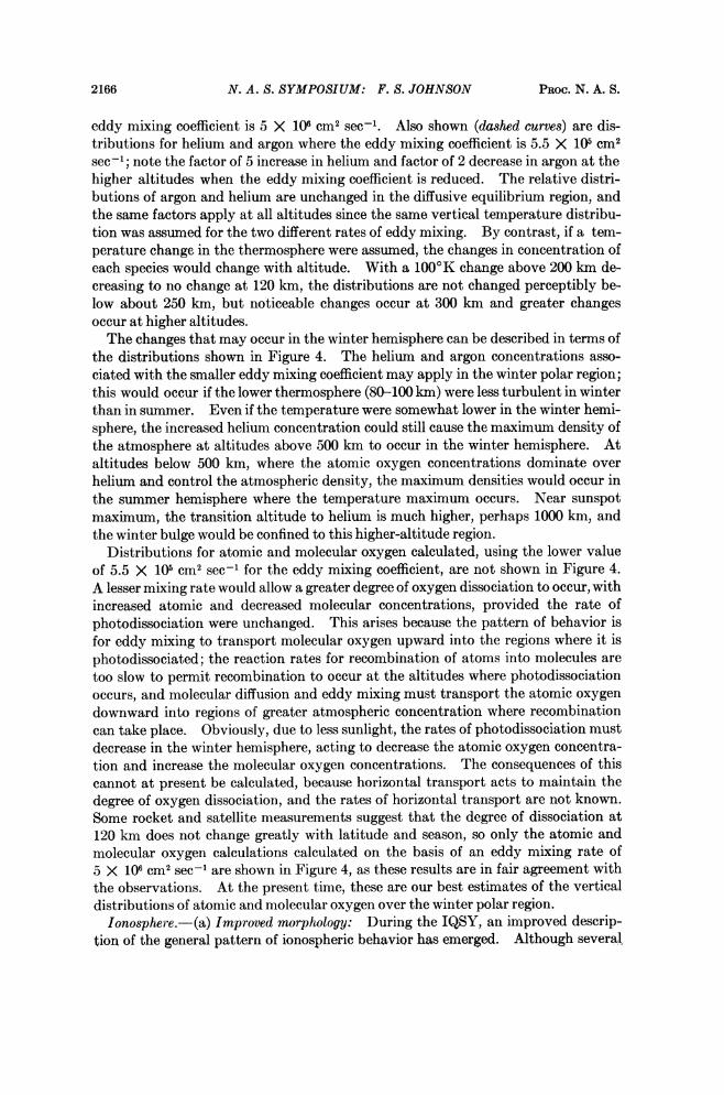
VOL. 58, 1967 A. S. SYMPOSIUM: F. S. JOHNSON 2169

but on either side of th( geomagnetic equator. A rather pronounced trough or rel-ative minimum exists along the geomagnetic equator during the afternoon, and theregions of maximum electron concentration occur as two somewhat elongatedmaxima symmetrically located about 150 north and south of the geomagnetic equator.Hanson and Moffett (1966) have explained this in terms of an eastward-directedelectric field that produces an upward drift of ionospheric plasma of about 10 msec'. The plasma then diffuses downward in the gravitational field along thegeomagnetic equator towards higher latitudes. Figure 7 shows the pattern oftransport, and Figure 8 shows the calculated ionization contours when photoion-ization, recombination, diffusion, and electromagnetic drift are taken into accountfor daytime conditions near the minimum of the solar cycle.The F region persists throughout the night. To explain this in terms of recom-

bination processes, the rate coefficients would have to be unreasonably small.Hanson and Patterson (1964) showed how the F region could be maintained throughthe course of the night with acceptable rate coefficients provided an electric fieldwere present that would cause an upward drift; the lesser densities that prevail atthe higher altitudes reduce the loss rate to a value that is consistent with the night-time persistence of the F region. This also provides a ready explanation for the F-region trough at 60° geomagnetic latitude if there is a mechanism to reverse theelectric field direction there. Since the electric fields are generated by motionsarising in the neutral atmosphere, the question resolves itself into one of a pattern ofatmospheric circulation.

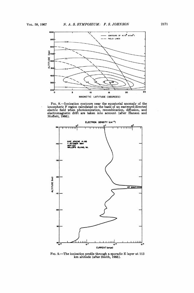
Sporadic E at temperate latitude has been identified as consisting of thin layers ofgreatly enhanced electron concentration, as indicated in Figure 9 (Smith, 1966). Amechanism to explain the formation of such a layer has been recognized by Axfordand Cunnold (1966). This depends upon the existence of a strong wind shear thatcauses the plasma above and below the shear to drift into the shear zone and in-crease in concentration there. Where several ion species are present, the morerapidly combining species are preferentially removed by recombination in the regionof the concentration increase, leaving the most slowly recombining species as theprincipal ion constituents in the thin sporadic E layer. The most slowly recom-bining ions in the ionosphere are metallic ions, probably of meteoric origin, but theyare normally of relatively minor importance. However, they become the predomi-nant ion in the sporadic E layer because of the selective removal of the ions thatnormally predominate in the E region-molecular oxygen and nitric oxide.

(c) Chemistry: There has been frequent disagreement in past years between re-combination rates and reaction rates derived from ionospheric data and those ob-tained from laboratory measurements for reactions that were thought to be perti-nent. Norton et al. (1963) have presented ionospheric evidence for reaction rates;in particular they noted the importance of the reaction

O+ + N2 -- NO+ + N

and that its reaction rate should be near 10-12 cm3 sec'. This has now been con-firmed by laboratory measurements by Ferguson et al. (1965a), who obtained avalue of 3 X 10-12 cm3 sec-. Ferguson et al. (1965b) have also measured the ratefor the reaction

N2+ + O- NO+ + N,

2170 N. A. S. SYMPOSIUM: F. S. JOHNSON PROC. N. A. S.

"0

0~~~~~~

eq~~~~0_0 0

0W~l) 3anl~lrv "

"0

0~~~~~~~~~~~~~~~

2 0~~~~~~~~I

C,-~~~~~~~~~~~~

Al~~~ ~ ~ ~ ~ ~ ~ ~ ~ ~ .00o~~~~~~~~~~~~~~~~~~~~~~~~~~~~~~~~~~~~~~~~~~~~~~~~~~~~~~~~~~~~~~~~~~~~~~~

0~~~~~~~~~~~~~~~~

o

K)~ ~ ~ ~ ~ (M ail

VOL. .58, 1967 N. A. S. SYMPOSIUM: F. S. JOHNSON 2171

1000 '\CONTOURS OF NO{1 el/cm3 )

900 \ - FIELD LINES-

80\-

E70i0:3600-

400-

aW_ 0.0

200)0 5 10 Is 20 25

MAGNETIC LATITUDE (DEGREES)

FIG. 8.-Ionization contours near the equatorial anomaly of theionospheric F region calculated on the basis of an eastward-directedelectric field when photoionization, recombination, diffusion, andelectromagnetic drift are taken into account (after Hanson andMoffett, 1966).

ELECTRON DENSITY (cm'a)

ISO so}10 106

NIKE APACHE 14.195140- 7 OCTOBER 9%

1804 ESTWALLOPS ISLAND, VA.

130C

120-

110

100 _

90

10.4 10' IO-$ 0-3CURRENT (amps)

FIG. 9.-The ionization profile through a sporadic E layer at 113km altitude (after Smith, 1966).

2172 N. A. S. SYMPOSIUM: F. S. JOHNSON PROC. N. A. S.

obtaining a value of 2.5 X 10-"' cm' see-'; this108000 ' \EL.ECTRON WHISTLER is the main loss process for N2+ between 120

6 - PROTON WHISTLER and 220 km, and it provides the main source of400 - __as NO+near140km.

L :200 z Plasma Properties.-(a) Ion whistlers: Ion0 > 2 3 cyclotron whistlers have been observed in satel-

TIME (secd lites (Gurnett and Shawhan, 1965). These are

FIG. 10.-The frequency-time char- signals that propagate below the ion gyro fre-acteristics of a proton whistler (after quency in the left-handed polarized mode. AnGurnett et al., 1966). Q, is the proton example is shown in Figure 10. The electrongyrofrequency and W12 is the cross-overfrequency. whistler in Figure 10 is a short fractional-hop

electron whistler propagating in the right-handpolarized whistler mode. At a cross-over frequency that occurs below the protongyrofrequency, the upgoing right-hand polarized whistler signal undergoes a polari-zation reversal to become a proton cyclotron whistler. Because of the presence ofheavier ions that would not permit the propagation of ion cyclotron waves withfrequencies greater than the heavy-ion cyclotron frequency, the mode can be ex-cited only by the polarization reversal mechanism at the cross-over frequency. Incommon with other whistlers, the maximum frequency is the gyrofrequency.

(b) Plasma line observation in Thomson scatter: Incoherent radar backscatter, orThomson scatter, from the ionosphere can be observed when powerful transmittersare used at frequencies far above the plasma frequency of the ionosphere. M\ost ofthe returned energy is in a narrow central line where the line width is governed bythe Doppler spread for the ion thermal velocities. However, a small amount of

30

50y\ a 6.2 MC/S - 20k A A ~~~~~scale40 __ M 10

30@ \ V * ~5.2 M/SS

CL10t - 40E

0or- 30

Z 50 _ - 20V *4.3 MdC / FIG. 11.-Plasma line observations in

.Z 40 -_ 10 Thomson scatter (after Perkins et al.,1965). The responses shown are those

z obtained through filters offset from the\0 0transmitter frequency by the amountsshown. Two peaks are seen for each

20 - \ uV3.9 MC/$ filter; these come from the two regions,scale one above and one below the ionization

lo _ maximum, where the plasma frequencyequals the difference between the trans-

X . |mitter frequency and the filter frequency.I00 200 300 400 500

Altitude - km

Vot. 58, 1967 N. A. S. SYMPOSIUM: F. S. JOHNSON 2173

power is returned in a pair of sharp lines separated from the transmitter frequencyby the plasma frequency. This has been observed by Perkins et al. (1965), andtheir results are shown in Figure 11. A filter is used which is offset from the trans-mitter frequency by the indicated amount. Two regions, one above the ion concen-tration maximum and one below it, give responses that fall within the bandpass ofthe filter, so two peaks are seen.The response seen in Figure 11 is greater than predicted by the theory for a

thermal plasma. Perkins and Salpeter (1965) have explained the enhancement interms of photoelectrons. Recently, they have observed differences between theupshifted and the downshifted frequencies that result from the greater number ofupward-moving (escaping) photoelectrons than downgoing photoelectrons thathave come from the magnetically conjugate point in the other hemisphere; this ob-servation indicates that there is significant scattering of photoelectrons in the mag-netosphere and that they cannot pass from one hemisphere to the other withoutsignificant attenuation.

Anderson, A. D., "An hypothesis for the semi-annual effect appearing in satellite orbital decaydata," Planet. Space Sci., 14, 849-861 (1966).

Axford, W. I., and D. M. Cunnold, "The wind shear theory of temperature zone sporadic E,"Radio Science, 1 (n.s.), 191-198 (1966).

Calvert, W., and T. E. Van Zandt, "Fixed frequency observation of plasma resonances in thetopside ionosphere," J. Geophys. Res., 71, 1799-1813 (1966).

Carpenter, D. L., "Whistler studies of the plasmapause in the magnetosphere, 1. Temporalvariations in the position of the knee and some evidence on plasma motions near the knee," J.Geophys. Res., 71, 693-709 (1966).

Ferguson, E. E., F. C. Fehsenfeld, P. D. Golden, and A. L. Schmeltekopf, "Positive ion-neutralreactions in the ionosphere," J. Geophys. Res., 70, 4323-4329 (1965a).

Ferguson, E. E., F. C. Fehsenfeld, P. D. Golden, A. I. Schmeltekopf, and H. I. Schiff, "Labora-tory measurements of the rate of the reaction N2 + +0 -O NO + + N at thermal energy," Planet.Space Sci., 13, 823-827 (1965b).

Gurnett, D. A., and S. D. Shawhan, "Ion cyclotron whistlers," J. Geophys. Res., 70, 1665-1688(1965).Hanson, W. B., and R. J. Moffett, "Ionization transport effects in the equatorial F region,"

J. Geophys. Res., 71, 5559-5572 (1966).Hanson, W. B., and T. N. L. Patterson, "The maintenance of the nighttime F-layer," Planet.

Space Sci., 12, 979-997 (1964).Jacchia, L. G., The Temperature above the Thermopause (Smithsonian Astrophysical Observa-

tory Special Report No. 150, 1964), 32 pp.Jacchia, L. G., and J. Slowey, The Shape and Location of the Diurnal Bulge in the Upper Atmo-

sphere (Smithsonian Astrophysical Observatory Special Report No. 207, 1966), 22 pp.Keating, G. M., and E. J. Prior, "Latitudinal and seasonal variations in atmospheric densities

obtained during low solar activity by means of the inflatable air density satellites," Seventh In-ternational Space Science Symposium of COSPAR, Vienna, 1966.

Keating, G. M. and E. J. Prior, "The distribution of helium and atomic oxygen in the exo-sphere," Trans. Am. Geophys. Union, 48, 188 (1967) (abstract).Muldrew, D. B., "F-layer ionization troughs deduced from Alouette data," J. Geophys. Res.,

70, 2635-2650 (1965).Nicolet, M., "Helium, an important constituent of the lower exosphere," J. Geophys. Res., 68,

2263-2264 (1961).Norton, R. B., T. E. Van Zandt, and J. S. Denison, "A model of the atmosphere and ionosphere

in the E and F, regions," in Proceedings of the International Conference on the Ionosphere, ed. A. C.Strickland (London: Inst. Phys. and Phys. Soc., 1963), pp. 26-34.

2174 N. A. S. SYMPOSIUM: F. S. JOHNSON PROC. N. A. S.

Perkins, F. W., and E. E. Salpeter, "Enhancement of plasma density fluctuations by non-thermal electrons," Phys. Rev., 139, A55-A62 (1965).

Perkins, F. W., E. E. Salpeter, and K. 0. Yngvesson, "Incoherent scatter from plasma oscilla-tions in the ionosphere," Phys. Rev. Letters, 14, 579-581 (1965).

Smith, L. G., "Rocket observations of sporadic E and related features of the E region," RadioScience, 1 (n.s.), 178-186 (1966).Van Zandt, T. E., B. T. Leftres, and W. Calvert, "Explorer XX observations at conjugate

ducts," in Report on Equatorial Aeronomy, ed. F. de Mendonga (Sio Paulo, Brasil: SAo Jos6 dosCampas, 1965), pp. 325-327.