research.engr.oregonstate.eduresearch.engr.oregonstate.edu/mpcl/resources/Paper_PersonalCopy.pdf ·...

1 23

The International Journal ofAdvanced Manufacturing Technology ISSN 0268-3768 Int J Adv Manuf TechnolDOI 10.1007/s00170-014-6386-2

A curvature optimal sharp cornersmoothing algorithm for high-speed feedmotion generation of NC systems alonglinear tool paths

Burak Sencer, Kosuke Ishizaki & EijiShamoto

1 23

Your article is protected by copyright and

all rights are held exclusively by Springer-

Verlag London. This e-offprint is for personal

use only and shall not be self-archived

in electronic repositories. If you wish to

self-archive your article, please use the

accepted manuscript version for posting on

your own website. You may further deposit

the accepted manuscript version in any

repository, provided it is only made publicly

available 12 months after official publication

or later and provided acknowledgement is

given to the original source of publication

and a link is inserted to the published article

on Springer's website. The link must be

accompanied by the following text: "The final

publication is available at link.springer.com”.

ORIGINAL ARTICLE

A curvature optimal sharp corner smoothing algorithmfor high-speed feed motion generation of NC systemsalong linear tool paths

Burak Sencer & Kosuke Ishizaki & Eiji Shamoto

Received: 30 April 2014 /Accepted: 10 September 2014# Springer-Verlag London 2014

Abstract Conventional tool paths for computer numerical-controlled (CNC) machine tools or NC positioning systemsare mainly composed of linear motion segments, or the so-called G1 commands. This approach exhibits serious limita-tions in terms of achieving the desired part of geometry andproductivity in high-speed machining. Velocity and accelera-tion discontinuities occur at the junction points of consecutivesegments. In order to generate smooth and continuous feedmotion, a geometric corner smoothing algorithm is proposedin this paper, which fits quintic B-splines to blend adjacentstraight lines together. The proposed transition scheme en-sures G2 continuity transitions and optimal curvature geome-try delivering fast cycle time without violating the axis accel-eration limits. The cornering error is controlled analyticallyallowing the user to set the desired cornering tolerance. Thefeed profile along the corner-blended tool path is generatedbased on S-curve-type acceleration profile, and it is scheduledfor minimum cycle time. At last, the corner-blended tool pathis interpolated in real-time with minimum feed fluctuation foraccurate and smooth feed motion. Proposed algorithms areimplemented, and their effectiveness is tested on a CNCmachine tool.

Keywords Machine tools . NC system . Trajectorygeneration . Bezier curve . Curvature

1 Introduction

With recent advances in part design and manufacturing tech-nologies, computer-aided design (CAD) systems are utilizedto design complex geometries compromised of smooth

parametric splines such a NURBS or B-splines [1]. Directinterpolation of these curves is proven to be superior in termsof providing smoother and faster motion [2–4]. However, vastmajority of numerical control (NC) units of machine tools orrobotic systems do not accept reference tool paths defined byhigh order parametric curves. One main reason for this is thelack of an established convention for the data transfer betweenCAD and NC. Another reason is implementation issues withinthe NC. Real-time interpolation of parametric curves stillexhibits some bottlenecks in terms of accurate computationof curve lengths [5] or the suppression of feed fluctuations [6,7]. Instead, given the tolerance, computer-aided manufactur-ing (CAM) systems are used to generate cutter location filescompromised of numerous short line segments, and NC sys-tems simply interpret these linear “point-to-point” motioncommands. Interpolating along those linear segments exhibitsserious limitations in terms of achieving the desired produc-tivity. The motion has to stop between each linear segmentblock due to the lack of higher order geometric continuity.This leads to elongated cycle times since the motion has toaccelerate and decelerate along each linear segment. On theother hand, if linear segments are travelled in constant feedmotion, there will be severe discontinuities in velocity andacceleration at junction points. This may excite motion sys-tems’ lightly damped structural modes and cause trackingerrors, both of which severely deteriorate the positioningquality [8].

In an attempt to generate smooth continuous motion alongseries of discrete linear motion commands, two major tech-niques have been proposed for modern NC systems. The firstone is geometric path smoothing where curve-fitting tech-niques are utilized to smoothen the discrete tool-path data.Advanced NC systems utilize approximate or exact splineinterpolation techniques to generate continuous trajectoriesfrom batch of linear point-to-point motion commands [9,10]. There exist several shortcomings when these methods

B. Sencer (*) :K. Ishizaki : E. ShamotoNagoya University, Nagoya, Aichi, Japane-mail: [email protected]

Int J Adv Manuf TechnolDOI 10.1007/s00170-014-6386-2

Author's personal copy

are applied. Firstly, higher order such as cubic (3rd) or quintic(5th) splines is necessary to generate C2, i.e. accelerationcontinuous, tool paths from given discrete data.Nevertheless, higher order splines may exhibit “wiggles”or “curls” when fitted along densely placed short linearmotion segments due to numerical conditioning. Thiscould be addressed utilizing some heuristic methods [11,12], or some energy functions based on pseudo jerk or thecurvature can be considered [13–15] for smoothness. Analternative is to approximate the discrete tool path byparametric splines. However, in this case, the control ofthe fitting error becomes computationally expensive forreal-time implementation.

Next, “corner blending,” also called the “corner smooth-ing,” techniques have been proposed to achieve nonstop con-tinuous motion. The idea is straightforward. Sharp corner isreplaced with a smooth parametric curve, as has already beenapplied in robotics literature [16]. Jouaneh et al. [17] replacedthe corner with a circular arc for fast cornering. However, acircular arc only delivers velocity continuous motion transi-tion. They later used a double (two) clothoid curves to furthersmoothen the motion transition [18]. These techniques arecomputationally less stringent and lead to more efficientreal-time implementation in the NC system. But, the order ofthe blending curve must be increased to control the fittingtolerance and the corner geometry at the same time. Yutkowitzand Chester [19] utilized two 4th order polynomials to realizecorner blending for Cartesian motion systems. This methoddelivers C2 continuous corner transition in the expense ofsignificant computational load. Pateloup et al. [20] proposeda 2-D path-smoothing method, which employs cubic B-splines with eight control points to round pocket profiles.Similarly, Zhang et al. [21] proposed a more general methodutilizing double cubic B-splines. Others [22, 23] also utilizedsimilar transition methods to achieve acceleration continuousfeed motion.

One of the vital aspects of corner smoothing is the design ofthe corner blend so that it can be traveled at high speed andthus the total cycle time could be minimized. In practice, aconventional tool path may contain thousands of linear seg-ments. Minimizing the cornering time spent at each corneractually presents a great potential to reduce overall machiningtime. However, limited effort has been directed toward thedesign of optimal corner geometry. Erkorkmaz et al. [24]considered dynamics of the servo system while designingthe corner blend. They found that over-corner spline deliversless cornering error but a longer cornering time. Beudaert et al.[25] addressed the problem of sharp corners in 5-axis motionutilizing a pair of B-spline curves. Zhao et al. [23] proposed areal-time cornering scheme where the curvature extremumcould be computed for fitted corner splines. They concludedthat optimization of the curvature in real-time is computation-ally stringent and unfeasible. Similarly, authors [26] have tried

to find real-time efficient optimization techniques. This paperproposes a “curvature optimal cornering scheme” wherethe maximum curvature of the corner is minimized in acomputationally efficient strategy that is suitable forreal-time implementation. This results in a high-speedcornering scheme and thus significant reduction in the totalcycle time.

Once the discrete tool path is blended with cornersplines, it becomes a mixture of linear segments contin-uously connected with blending splines. The next prob-lem is scheduling of the feedrate profile along the toolpath. Due to curved corner profile, tangential feed mustbe lowered so that axis velocity and acceleration limitsare not violated at corner sections. Therefore, high-speed feed sections of linear segments must be stitchedtogether with low-speed cornering segments while en-suring that the kinematic compatibility conditions be-tween position, velocity, acceleration, and jerk are notviolated. Several feed profiles have been suggested inthe literature to smoothly schedule the tangential speed[27, 28]. Comprehensive feedrate optimization tech-niques have also been introduced for complex splinetool paths [29–31] to minimize the cycle time whilerespecting physical limits of the drives. As comparedto the current literature, the work in this paper utilizessmooth S-curve-type acceleration transitions while con-sidering the kinematic compatibility conditions betweenadjacent feed segments. An efficient algorithm is pro-posed for federate scheduling along the entire tool pathconsidering the maximum cornering speed while re-specting the acceleration limits of the drives.

At last, the tool path must be interpolated with respect tothe feedrate profile in real-time to generate axis referencecommands. In order to smoothly interpolate the referencetrajectory without any feedrate fluctuations, the recursive in-terpolation scheme developed in a previous study [7] forparametric splines is applied on quintic Bezier cornerblends.

This paper presents methods to overcome some of theinefficiencies in current corner smoothing techniques andpresents a computationally efficient curvature optimal cornersmoothing algorithm for high-speed machine tools and mo-tion systems to attain minimum cycle time motion. The over-all corner smoothing scheme is summarized in Fig. 1. Oncethe discrete tool path is generated by CAM systems, proposedcorner smoothing algorithm utilizes a single quintic Bezierspline to ensure G2 continuous motion transition betweenlinear segments. The corner curvature is optimized to deliverminimum curvature extremum and thus realizes rapidcornering speed using less acceleration/torque capacities ofthe axes in motion. Next, S-curve-type acceleration transientsare designed to stitch feed segments smoothly along multi-segmented tool path, and a feedrate-scheduling algorithm is

Int J Adv Manuf Technol


presented to plan the feed motion along multi-segmented toolpath. Finally, it is interpolated in real-time and validatedexperimentally on a 3-axis Cartesian machine tool.

2 Smoothening of sharp corners

Two consecutive linear segments are blended withBezier splines as shown in Fig. 2a to deliver a smoothtransition of feed motion from one linear segment to thenext. A quintic Bezier segment (see in Fig. 2b) inCartesian coordinates can be defined parametrically asfollows:

B uð Þ ¼Bx uð ÞBy uð ÞBz uð Þ

24

35 ¼ 1−uð Þ5P0 þ 5u 1−uð Þ4P1 þ 10u2 u−1ð Þ3P2

þ10u3 1−uð Þ2P3 þ 5u4 1−uð ÞP4 þ u5P5

� �and

P0 ¼P0;x uð ÞP0;y uð ÞP0;z uð Þ

24

35;P1 ¼

P0;x uð ÞP0;y uð ÞP0;z uð Þ

24

35;…;P5 ¼

P5;x uð ÞP5;y uð ÞP5;z uð Þ

24

35

ð1Þ

where Bx, By, and Bz are the axis position polynomials. P0,P1,…, P5 are the vectors containing control points for eachaxis coordinate. u is the Bezier curve parameter, u∈[0,1]. Asobserved from Eq. 1, there are six control points in the

proposed Bezier blend that needs to be determined to ensurethe following:

(i) Smooth transition between linear segments, namely G2

continuous motion

(ii) Minimum curvature extremum for the fastest corneringspeed

(iii) Accurate control of the cornering error to respect themanufacturing tolerances

2.1 Design of the quintic Bezier blend

The quintic Bezier blend is applied in transition of twopoint-to-point linear motion segments as shownin Fig. 2c. Pstart is the starting point of the kth linearsegment, Ptrans is the ending point, which becomes thetransition point to the (k+1)th segment, and θ is thecornering angle. In blending two consecutive linearsegments, G2 continuity is ensured so that twosuccessive segments share the same tangent and normaldirections at the junction points. Combined withaccurate interpolation presented in later sections,this allows the realization of C2 motion. Differen-tiating Eq. 1 with respect to the spline parameter ugives the 1st and 2nd derivative profiles along the Bezierblend:

Fig. 1 Proposed corner smoothing scheme



Bu ¼ dB uð Þdu

¼ 5 1−uð Þ4 P1−P0ð Þ þ 20u 1−uð Þ3 P2−P1ð Þ þ 30u2 u−1ð Þ2 P3−P2ð Þþ20u3 1−uð Þ P4−P3ð Þ þ 5u4 P5−P4ð Þ

Buu ¼ d2B uð Þdu2

¼ 20 1−uð Þ3 P2−2P1 þ P0ð Þ þ 60u 1−tð Þ2 P3−2P4 þ P5ð Þ

9>>>>=>>>>;

ð2ÞEvaluating the profiles from Eqs. 1 and 2, at the start u=0

and end u=1 of the Bezier blend reveals

Bju¼0 ¼ P0;Buju¼0 ¼ 5 P1−P0ð Þ

Buuju¼0 ¼ 20 P2−2P1 þ P0ð Þ

9=; and

Bju¼1 ¼ P5;Bujuu¼1 ¼ 5 P5−P4ð Þ

Buuju¼1 ¼ 20 P5−2P4 þ P3ð Þ

9=; ð3Þ

As observed fromEq. 3, P0 and P5 define junction points ofthe Bezier blend to linear segments. In this design, they areplaced at a Euclidian distance, 2c+d away from the cornertransition point, Ptrans as

P0 ¼ Ptrans− 2cþ dð Þts and P5 ¼ Ptrans þ 2cþ dð Þtegð4Þ

where ts and te are the unit tangent vectors along linearsegments,

ts ¼ Ptrans−Pstart

Ptrans−Pstartk k and te ¼ Pend−Ptrans

Pend−Ptransk k ð5Þ

Tangent vectors on the junction points of the Bezier can bealigned to linear segment by simply placing P1 and P4

anywhere along ts and te. They are placed at a distance of cfrom the junction points as

P1 ¼ P0 þ cts andP4 ¼ P5−cteg ð6Þ

Please note that this only ensures G1 continuity since onlythe tangent directions are matched but not their magnitude.Next, in order to satisfy curvature continuity, normal vectors atthe junction points, Buu|u=0 and Buu|u=1, must be zero.According to Eq. 3, this can be achieved by satisfying

Buuju¼0 ¼ 20 P2−2P1 þ P0ð Þ ¼ 0 → P1−P0 ¼ P2−P1

Buuju¼1 ¼ 20 P5−2P4 þ P3ð Þ ¼ 0 → P4−P5 ¼ P3−P4

�ð7Þ

Substituting Eq. 7 into Eq. 4 yields

P0 þ 2cts ¼ P2; and P5−2cte ¼ P3 g ð8Þ

which reveals that the control points P1 must be placedcollinear with P0 and P2, and P3 with P4 and P5. FromEqs. 6 and 8, all six control points of the Bezier blendare determined as

P0 ¼ Ptrans− 2cþ dð Þts P5 ¼ Ptrans þ 2cþ dð ÞteP1 ¼ P0 þ c ts P4 ¼ P5− c tsP2 ¼ P0 þ 2 c ts P3 ¼ P5− 2 c ts

9=; ð9Þ

making the corner blend symmetric with respect to the angularbisector of the two lines PstartPtrans and PtransPend, and G2

continuous to the neighboring segments.

2.2 Curvature optimization

Curvature is solely a function of the path geometry, and it isintegrally tied to the acceleration and jerk required to track thecorner geometry. In high-speed machining, it is desirable tomaximize the total cornering speed while still respecting theactuator acceleration. The curvature along the path is definedas follows [32]:

κ ¼ dTds

��; T ¼ tx; ty; tz

� �T3�1 ð10Þ

where T is the unit tangent vector and s is the arc displace-ment. The relationship between the differential arc displace-ment ds and the Bezier parameter increment du can be derivedas

ds ¼ Buk kdu ð11Þ

Furthermore, as the curve is traveled along, change in theunit tangent vector as a function of time can be expressed byapplying the chain rule to Eq. 10:

Fig. 2 Quintic Bezier corner blending



dTdt

�� ¼ dT

ds

ds

dt

�� ¼ κv ð12Þ

where v ¼ s ¼ ds=dt is the tangential or the path velocity.Please note that the derivative of the unit tangent vector, dT/dt,is orthogonal to itself. Therefore, the path normal can also bewritten as a function of time:

N ¼ 1

dT=dtk kdTdt

ð13Þ

Axis velocity v=[vx,vy,vz]T and acceleration a=[ax,ayaz]

T

components are written from Eqs. 12 and 13 as

v ¼ vTand

a ¼ d

dtvTð Þ ¼ dv

dtTþ v

dTdt

9=; ð14Þ

and from Eq. 14 the effect of curvature on the axis accelera-tions is derived as

a ¼ �vTþ v2κN ð15Þ

The �v ¼ s:: ¼ dv=dt term represents tangential or the so-called path acceleration. Assuming that the corners are turnedat constant speed, that term vanishes relating the axis acceler-ations directly to the path velocity, v and the curvature as

a ¼axayaz

24

35 ¼ v2κN ð16Þ

Thus, the objective hereby is to minimize curvature extre-mum, i.e., the maximum of the curvature along the Bezierblend, so that the cornering speed can be increased while stillstaying within the acceleration limits of drives.

In the proposed Bezier corner blend design, the shape ofthe Bezier, i.e., the control point locations, is controlled by theEuclidian distances c and d. Figure 3 shows the effect of c andd on the Bezier shape for a cornering angle of 60° whenjunction points (P0 and P5) are fixed. As illustrated, by keep-ing the junction points fixed and increasing d, control pointsare pushed away from corner transition point Ptrans leading tolarger cornering errors. Increasing c leads to smaller fittingerrors but in contrary may generate larger curvature radiusdepending on d. Thus, the optimal ratio of c/d is searched forminimizing the curvature extremum. Curvature along theBezier can be written analytically from Eqs. 2, 10, and 11 asa function of the curve parameter, u:

κ ¼ −12nusinθ 2nþ 1ð Þ u−1ð Þ nu−2u−2nu3 þ nu4 þ 4u3−2u4 þ 1ð ÞLTA

32

ð17Þ

where n=c/d, LT=2c+d, and A=A(u) is an 8th order polyno-mial. Please refer to the Appendix section for detailed deriva-tion of Eq. 17. As noted, curvature is affected by the corneringangle, θ, n, and also the total transition length LT, which simplyscales the curvature in this design. The optimal n value forvarious cornering angles can be searched to minimize thecurvature extremum from Eq. 17. Nevertheless, this operationmay be computationally expensive considering the fact that itneeds to be implemented in real-time for each and everycorner. This bottleneck has also been stated previously in thedesign of corner blends [22, 23]. Instead of solving the opti-mization problem in real-time, a more practical approach ispursued here.

Since the cornering distance LT simply functions as ascaling factor in the proposed design, it is set to unity

LT ¼ 2cþ d ¼ 1 ð18Þ

and only the effect of n=c/d considered. The corner angle θ isfixed, and n is interpolated in the range of n∈[0,2]. Curvatureis computed along the Bezier, at 100 discrete points propor-tional to the spline parameter, and its maxima is detected.

Figure 4 shows the change of maximum curvature, κmax.As shown, since Bezier blend is symmetric with respect to theangular bisector of the neighboring segments, maximum cur-vature occurs either in the middle of the Bezier, or twoidentical curvature extrema are observed. This vaguely indi-cates that the problem is convex, and there is a global optimaln value, which minimizes the maximum value of the curva-ture. The process is repeated for various cornering angles torecord the optimal n. Figure 5 shows the n value for a widerange of cornering angles θ=10….150°, which minimizes themaximum curvature. A simple power regression is applied toobtain the following relation to estimate the curvature optimaln value for a wide range of cornering angles as

n θð Þ ¼ 1

2:0769θ0:9927 ð19Þ

Equation 19 can be used in real-time to efficiently lookupthe optimal control point ratio, n, to fit the curvature optimalBezier blend.

2.3 Control of the cornering errors

As shown in Fig. 2c, proposed corner smoothing algorithmintroduces geometric errors, ε, around the corner, which has tobe limited by a given tolerance so that the dimensional integ-rity of the produced part is ensured. The Bezier blend issymmetric, and hence the maximum deviation from originalpath occurs in the middle at u=0.5,

ε ¼ Ptrans−Bju¼0:5

�� ð20Þ



The midpoint of the BezierB|u=0.5 is evaluated from Eqs. 1and 9 as

Bju¼0:5 ¼ Ptrans þ 7cþ 16d

32ts þ teð Þ ð21Þ

The maximum cornering error is then computed fromEqs. 20 and 21 as

ε ¼ 7nþ 16

32d ts þ tek k ð22Þ

Equation 22 is further expanded, and actual values of c andd for a curvature optimum Bezier blend at a given corneringtolerance ε and corner angle θ are obtained as

d ¼ 32ε

7nþ 16ð Þ ffiffiffiffiffiffiffiffiffiffiffiffiffiffiffiffiffiffiffiffiffiffiffi2þ 2cos θð Þp

c ¼ 32ε

7nþ 16ð Þ ffiffiffiffiffiffiffiffiffiffiffiffiffiffiffiffiffiffiffiffiffiffiffi2þ 2cos θð Þp n

ð23Þ

The actual transition length can then be evaluated asLT=2c+d.

3 Jerk-limited trajectory generation

Based on the developed corner smoothing algorithm inSection 2, a jerk-limited trajectory generation algorithmis proposed in this section. The objective is to modulatethe path speed in such a way that the velocity isreduced at corners i.e. along Bezier segments and againraised at linear segments to reach the programmedspeed. The proposed trajectory generation algorithmcan be implemented in real-time within a look-aheadscheme, or it can be used off-line for simulating themotion of computer numerical-controlled (CNC) sys-tems. The overall algorithm has three sections. At first,corners are rounded with Bezier blends, and the maxi-mum feedrate for each corner is determined. Next, thejerk-limited feedrate profile with S-curve-type accelera-tion transients is planned, and it is optimized so that thetotal cycle time is minimized while respecting the axisvelocity and acceleration limits. At last, the geometrictool path is interpolated in real-time without any feedfluctuation.

3.1 Determination of the maximum cornering speed

Conventional tool paths contain series of linear segmentswhere each segment has its Euclidian length and afeedrate assigned to it. Once the proposed corner smooth-ing approach is implemented, corners are blended andsegment lengths are altered. Figure 6 illustrates a planartool path consisting of linear segments. The total length SLof a tool path with Ns linear segments is computed con-sidering length of each block:

SL ¼X1

Ns

Pkþ1−Pkk k ð24Þ

Due to corner blending, tool-path length is updated bysubtracting corner transition length, LT, and adding the lengthof the Bezier blend, LB, as

SΣ ¼ SL þXNs−1

1

LB;k−2LT ;k� ð25Þ

where LB is computed through numerical integration as fol-lows. The Bezier blend is divided intoM (>100) subdivisionsproportional to its parameter u, and the corresponding axispositions are computed as

Fig. 4 Corner curvature for various cornering angles and control pointratios

Fig. 3 Effect of n on the Bezier curvature (θ=60°)



x j ¼ 1−jΔuð Þ5P0;x þ 5jΔu 1−jΔuð Þ4P1;x þ…þ jΔu5P5;x

y j ¼ 1−jΔuð Þ5P0;y þ 5jΔu 1−jΔuð Þ4P1;y þ…þ jΔu5P5;x

z j ¼ 1−jΔuð Þ5P0;z þ 5jΔu 1−jΔuð Þ4P1;z þ…þ jΔu5P5;z

9>=>;;

Δu ¼ 1

M; j ¼ 0; 1…M

The resulting arc increments are then summed up:

LB ¼Xj¼1

M

Δsk; j

¼Xj¼1

Mffiffiffiffiffiffiffiffiffiffiffiffiffiffiffiffiffiffiffiffiffiffiffiffiffiffiffiffiffiffiffiffiffiffiffiffiffiffiffiffiffiffiffiffiffiffiffiffiffiffiffiffiffiffiffiffiffiffiffiffiffiffiffiffiffiffiffiffiffiffiffiffiffiffiffiffiffiffiffiffiffiffiffiffiffiffiffiffixk; j−xk; j−1� 2 þ yk; j−yk; j−1

�2þ zk; j−zk; j−1� 2r

ð27Þ

Next, due to curvature of the Bezier blend, axis accelera-tion limits may be violated if the curved sections were also tobe traveled at the same speed of neighboring linear segments.The highest cruise speed along a Bezier blend is bounded bythe acceleration limits Ax,max, Ay,max, and Az,max of the drives.Equation 16 is used to determine the highest cornering speedas

Fcorner ¼ minAx;max

κmax;Ay;max

κmax;Az;max

κmax

� �ð28Þ

A case study is shown in Fig. 6. The desired feedrate for thelinear tool path is given as F=35 mm/s. The tool path issmoothened at two different cornering tolerances namely,100 and 150 μm. As shown, depending on the corner toler-ance, the transition length LT changes. For tighter corneringtolerance, LT becomes smaller and thus the maximum

curvature is larger. Figure 6b shows the highest corneringspeed for different cornering tolerances. It can be noted thatthe maximum cornering speed reduces as the cornering toler-ance becomes tighter.

3.2 Feedrate scheduling

As presented in the previous section, when linear segments arejoined with Bezier blends, corners can only be traveled at amuch lower speed then their neighboring segments. The mo-tion system has to slow down when approaching to a corner,cruise the Bezier blend and accelerate to the programmed feedof the successive linear segment. In order to achieve smoothmotion, feed commands of consecutive segments must bestitched together smoothly. Speed transitions across blocksare achieved through a jerk-limited acceleration profile.Compatibility of the feedrates with respect to accelerationand jerk constraints given by the process planner are consid-ered, and a practical feed planning scheme is developed asfollows.

A jerk-limited motion profile or the so-called S-curve-type acceleration profile is utilized to generate smoothspeed transition between the two adjacent feed blocks.The feedrate profile for velocity transition is shown inFig. 7, and the corresponding acceleration function isdefined as

a tð Þ ¼ 30ΔVt4

t5e−60ΔV

t3

t4eþ 30ΔV

t2

t3eð29Þ

where ΔV=Fk+1−Fk is the velocity difference to be coveredfrom current kth segment to the consecutive (k+1)th and te istotal time spend in speed transition. Position (s), velocity (v),acceleration (a), and jerk (j) profiles can be obtained fromEq. 29 as

s tð Þ ¼ Fkt þ 5

2ΔV

t4

t3e−3ΔV

t5

t4eþΔV

t6

t5e

v tð Þ ¼ Fk−10ΔVt3

t3eþ 15ΔV

t4

t4eþ 6ΔV

t5

t5e

a tð Þ ¼ 30ΔVt2

t3e−60ΔV

t3

t4e−30ΔV

t4

t5e

j tð Þ ¼ 60ΔVt

t3e−180ΔV

t2

t4eþ 120ΔV

t3

t5e

9>>>>>>>>>>>=>>>>>>>>>>>;

ð30Þ

The total transition time, te, needs to be determined insuch a way that the tangential acceleration and jerk limits,Amax and Jmax, are not exceeded. As observed from Fig. 7,

Fig. 5 Optimal n w.r.t. cornering angle

ð26Þ



tangential acceleration peaks at t=½te. Thus, the speed tran-sition interval te

Amax with respect to acceleration limit can becomputed from Eq. 30 as

Amax ¼ 15

8

ΔVj jte

→tAmaxe ¼ 15

8

ΔVj jAmax

ð31Þ

Similarly, tangential jerk prolife peaks at t=¼te, and thespeed transition interval w.r.t. jerk limit is calculated as

Jmax ¼ 45

8

ΔVj jt2e

→t Jmaxe ¼

ffiffiffiffiffiffiffiffiffiffiffiffiffiffiffiffiffi45

8

ΔVj jJmax

sð32Þ

In order to respect both limits, the transition interval isdetermined as

te ¼ max tAmaxe ; t Jmax

e

� ð33Þ

Finally, the total displacement spent during a speed transi-tion is computed from Eqs. 30 and 33 as

ΔS ¼ Fkþ1 þ Fk

2te ð34Þ

Feed transitions are dictated by desired speeds of theneighboring segments and the total displacement traveledwithin the speed transition. The “kinematic compatibility”is defined here as having sufficient travel length tosmoothly change the feedrate, i.e., accelerate or decelerate,between segments [31]. If kinematic compatibility is

achieved, then displacement, feedrate, and accelerationprofiles will be continuous, and along with the jerk pro-file, they will be limited. Figure 8 illustrates the impor-tance of the kinematic compatibility. In Fig. 8a, speedincrease from low- to high-speed segment is shown whereFk<Fk+1. Please note that speed cannot be increased fromwithin the current, kth segment, since the current segmentfeed is lower. In other words, acceleration can only beplanned after slow feed segment is traveled. Thus, speedtransition is planned in the successive (k+1)th segment,and the compatibility condition is checked as

Lkþ1−Fk þ Fkþ1

2te;k ≥0;

where te;k ¼ max15

8

ΔVkj jAmax

;

ffiffiffiffiffiffiffiffiffiffiffiffiffiffiffiffiffiffiffi45

8

ΔVkj jJmax

s !ð35Þ

Fig. 6 Corner smoothened tool path

Fig. 7 S-curve-type acceleration profile for velocity transition



and ΔVk=Fk+1−Fk and Lk+1 is the length of the (k+1)th

segment. Figure 8b shows a velocity transition from high tolow speed. In this case, all the planning is performed withinthe current kth segment, and the compatibility conditions arechecked as

Lk−Fk þ Fkþ1

2te;k ≥0 ð36Þ

In general cases, feed transitions spread across seg-ment boundaries, and two adjacent segments may affectkinematic compatibility in the kth segment. In order toascertain whether kinematic compatibility is satisfiedacross the segment boundaries, previous and next seg-ments also need to be tested against the feed compati-bility conditions. Figure 8c simply illustrates this wherea high-speed block is neighbored by two low-speedsegments, which could be either linear or Bezier seg-ment. In this case, all the acceleration transition must beplanned within the kth segment, and the compatibilityconditions can be written as

Lk−Fk−1 þ Fk

2te;k−1 þ Fk þ Fkþ1

2te;k

� ≥0 ð37Þ

If Eq. 37 cannot be satisfied, achievable speed of thesegment k must be lowered so that the speed transitionfrom and to the segments k−1 and k+1 is achieved. Insimple cases, maximum speed along the Bezier blendscan be computed in a forward traversal search algo-rithm, and the compatibility conditions from the startto the end of the tool path are checked. If a violationoccurs, feedrate of the current block is reduced until itsatisfies the compatibility conditions with its neighbor-ing blocks. However, in a large-scale tool path compro-mised of many blocks, a compatible solution may notbe acquired given the commanded feed, acceleration,and jerk values. In such circumstances, violations canonly be corrected by tracing back the feedrate throughthe planned feed values and perform adjustment toearlier segments. A practical search algorithm is imple-mented here to efficiently generate a kinematically com-patible feed profile. The proposed algorithm can be usedoffline for the entire tool path all at once, or it can beimplemented in a windowing fashion for real-time exe-cution. The feed planning algorithm is presented asfollows:

Step 1 All the feeds in a scheduling window are initiated to aconservative feed value, Fk=vstart where k=1…N.

Step 2 Compatibility conditions are checked for each blockcounting in forward and backward directions simul-taneously. If the there is no kinematic violation in anyblock, all the block feeds are updated gradually bythe amount of dv, Fk=Fk+dv and the velocity incre-ment for the next round is doubled, dv=2dv.However, if there is any kinematic violation for ablock, the velocity increment is reduced by half,dv=dv/2 and the feedrates are updated.

Step 3 If the kinematic violation persists in a segment, itsfeedrate is frozen, and the rest of the blocks areupdated with the current feed increment, dv. If theviolation still persists at a certain block, in this case,the neighboring block feedrates are also frozen, andthe remaining feedrates are updated.

Step 4 The feed update continues, and the final feed profileis generated when all the block feedrates are frozenand cannot be updated.

The proposed feedrate scheduling technique is appliedon the tool path shown in Fig. 6a. The cornering toleranceis set to 25 μm and desired feedrate is set to F=35 mm/s.Tangential acceleration and jerk limits are set to1,500 mm/s2 and 20 × 104 mm/s3, respectively.Acceleration limits of the drives are also set to Ax,max=Ay,max=1,500 mm/s2, and the resultant feed profile isshown in Fig. 9a. As observed, segments are connectedto each other with smooth acceleration transients, andcorner segments are traveled at lower speeds consideringacceleration limits of the drives. Furthermore, due to lowacceleration and jerk limits, desired tangential feedratecould not be reached along the tool path. In Fig. 9b, thelimits are increased to Amax=Ax,max=Ay,max=2,000 mm/s2

and Jmax=40×104 mm/s3. In this case, desired feed could

be reached.

3.3 Real-time interpolation

After smoothing the given discrete path with Bezier blends,the new tool path is composed of linear and Bezier segments,and care must be taken while interpolating the mixed trajec-tory. Linear segments can simply be interpolated with linearinterpolation:

x kTsð Þy kTsð Þz kTsð Þ

24

35 ¼ Pk þ Pkþ1−Pk

Pkþ1−Pkk ks kTsð Þ; k ¼ 0…N ð38Þ

where s(kTs) is the displacement profile sampled at samplingtime of the interpolator, Ts, and N is the number of interpola-tion samples. However, since Bezier curves are not arc lengthparameterized [31], feedrate fluctuations will occur if it is



interpolated by applying constant parameter increments Δu,which are proportional to the desired arc increment Δs in theform

Δu ¼ 1

LBΔs ð39Þ

Furthermore, only G2 continuity is pursued while fitting theBezier curve to the sharp corners. As a result, while traveling atconstant speed, severe feed fluctuations may occur at thetransition points from linear to Bezier segments since themagnitude of tangent vector of the Bezier at the junction pointsis not matched. Such discontinuity will result in high frequencyacceleration and jerk harmonics and will cause unwanted vi-brations exciting structural modes of the drive system. Taylorapproximation has been used in general practice to interpolateparametric curves, which may fail to work when crossing fromthe linear segment to the Bezier segments at high speed [31]. Inorder to avoid such problems, the iterative spline parametercomputation technique from Erkorkmaz and Altintas [7] isapplied to accurately interpolate the Bezier blends. The ideais to solve the value of Bezier parameter Δu to realize thedesired arch displacement Δs. The arc increment Δstest corre-sponding to the tested spline parameter utest is estimated bycomputing the resulting axis increments:

Δstest ¼ffiffiffiffiffiffiffiffiffiffiffiffiffiffiffiffiffiffiffiffiffiffiffiffiffiffiffiffiffiffiffiffiffiffiffiffiffiffiffiffiffiffiffiffiffiffiffiffiffiffiffiffiffiffiffiffiffiffiffiffiffiΔxtestð Þ2 þ Δytestð Þ2 þ Δytestð Þ2

qwhere :Δxtest ¼ xtest−xprev ; Δytest ¼ ytest−yprev; Δztest ¼ ztest−zprevxtest ¼ 1−uð Þ5P0;x þ 5u 1−uð Þ4P1;x þ…þ u5P5;x

ytest ¼ 1−uð Þ5P0;y þ 5u 1−uð Þ4P1;y þ…þ u5P5;x

ztest ¼ 1−uð Þ5P0;z þ 5u 1−uð Þ4P1;z þ…þ u5P5;z

9>>>>>>>>=>>>>>>>>;

ð40Þ

where xprev, yprev, and zprev are the axis commands applied inthe previous control sample. The error between the desiredand tested arc increments is

e ¼ Δsdes−Δstest ð41Þ

and its gradient with respect to the tested spline parameter isderived using Eqs. 39 and 41 as

de

dutest¼

ΔxtestΔxtestΔu

� þΔytest

ΔytestΔu

� þΔztest

ΔztestΔu

� Δstest

ð42Þ

where (dxtest/du), (dytest/du), and (dztest/du) are simply obtain-ed by substituting the calculated value of utest into the deriv-ative expressions given in Eq. 2. The correct value of thespline parameter is computed with regard to the convergenceof the below iteration (i):

utestð Þiþ1 ¼ utestð Þi−ei

de=dutestð Þið43Þ

The desired convergence is achieved when the arc incre-ment error e is below 10−8 in Eq. 43. Since the Bezier blend issmooth and does not show sharp changes in the curvature, theinitial guess for utest can be obtained through linear approxi-mation of the nonlinear relationship between the arc length sand spline parameter u from Eq. 38. Depending on the avail-ability of a close initial guess and an analytical gradientenables Eq. 43 to converge reliably, within five iterations, ateach trajectory interpolation cycle.

4 Simulation and experimental results

The proposed corner smoothing technique is tested throughsimulations and experimentally validated. At first, a simula-tion study is performed to illustrate the effect of curvatureoptimized corner smoothing. Experimental tracking experi-ments are then conducted on a conventional CNC machinetool controlled by in-house developed NC system.

4.1 Simulation results

A 2-D rectangular tool path shown in Fig. 10 is smoothenedwith quintic Bezier blends. The cornering tolerance is selectedas 150 μm, and the corner points are indicated as Pk, k=0,

Fig. 8 Compatibility conditions along successive segments



1,…, 4. All the corner angles are 90° for this tool path,and they are smoothed with both using curvature optimaland nonoptimal Bezier blends. In the proposed curvatureoptimal Bezier blending method, the optimal controlpoint ratio, n=1.3265, is looked up efficiently fromEq. 19. In the remaining two cases, n is selected greaterand smaller than the optimal value. Figure 10b shows thechange in the curvature. As noted, proposed blendingtechnique ensures G2 continuity where curvature at thejunction points is zero for any n. In addition, when theoptimal corner ratio is utilized, it delivers the smallestcurvature extremum. The feedrate profile along the toolpath is then generated as presented in Section 3, andpresented in Fig. 11. As observed, when the curvatureis not optimized along the Bezier, the cornering feedratesare conservative. Total cycle time for the proposed cur-vature optimized method is the smallest TΣ=0.3655 s ascompared to the nonoptimal cases where the cycle timesare TΣ=0.3874 s at n=0.6878 and TΣ=0.3691 s at n=1.9652. This proves that the proposed Bezier cornersmoothing method can deliver curvature continuous cor-ner smoothing with minimum curvature extremum for thefastest cornering.

4.2 Experimental results

A commercial CNC machine tool is retrofitted to imple-ment the proposed corner smoothing algorithms shown inFig. 12. The conventional NC system is cancelled byswitching the amplifiers of the machine into torque mode

and modifying the PLC. Encoder feedback is taken fromthe motor side rotary encoders, and torque commands aredirectly send to the amplifiers. dSpace® real-time controlsystem is utilized and P-PI cascade controllers are imple-mented for each axis for accurate position control. Thetrajectory is generated off-line in MATLAB® environ-ment, and it is interpolated in real-time at the closed loopcontrol interval of 10 kHz.

A realistic case study is presented to validate the effec-tiveness of the proposed sharp corner smoothing algorithmon a complex planar tool path shown in Fig. 13. The toolpath consists of 126 linear segment lengths varying from3 mm to 13 mm. The desired travel speed for each line isF=100 mm/s, maximum path acceleration is Amax=2,500 mm/s2 and jerk is set to be maximum Jmax=20×104 mm/s3. The x- and y-axis acceleration limits are select-ed identical to the tangential acceleration Amax=Ay,max=Amax=2,500 mm/s2.

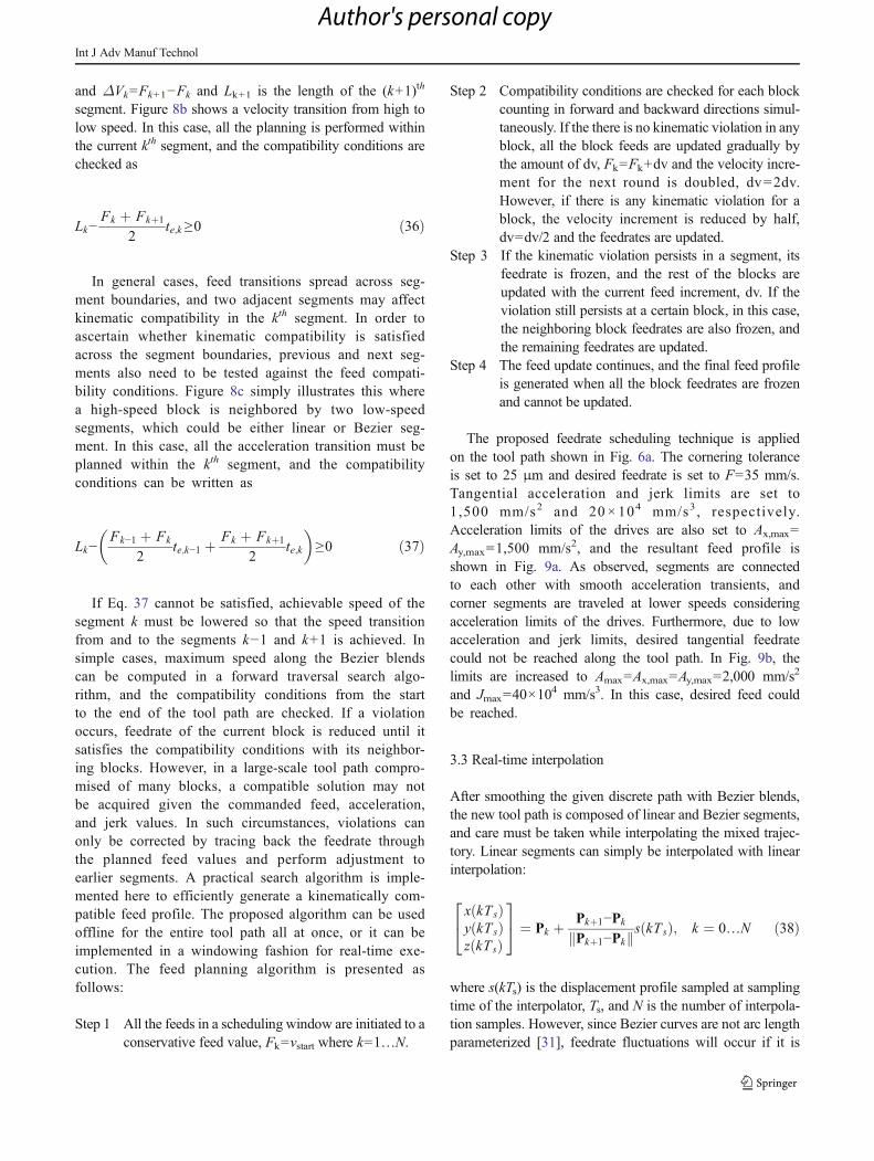
The tool path is traveled at three different trajectorygeneration strategies. Firstly, if the proposed cornersmoothing technique is not applied, the motion mustbe commanded to perform an instantaneous stop at theend of each linear segment since the linear segmentsonly ensure position continuity. In this case, the jerk-limited acceleration profile is utilized to plan the feedmotion along each linear segment individually, and thepoint-to-point trajectory is generated. The resultant tan-gential feed profile and axis kinematics are shown inFig. 14. As shown, servo system undergoes instanta-neous stops at the junction points (see Fig. 14a).Please note that the path speed only reaches thecommanded feed at longer linear segments due to thelimited acceleration of the drives. Since linear tool pathhas zero curvature, axis accelerations and velocities nev-er exceed given bounds as shown in Fig. 14b. The totalcycle time is 13.39 s.

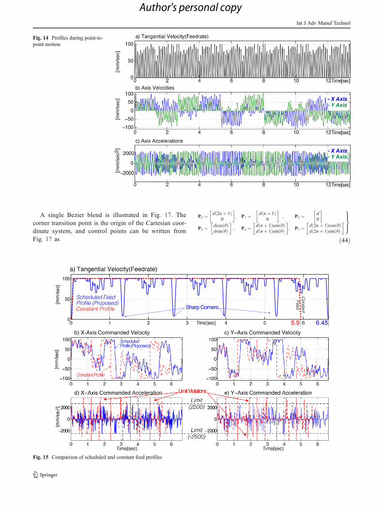
Next, the proposed corner smoothing technique is im-plemented. The cornering tolerance is set to ε=100 μm,and the tool path shown is smoothened. Since the tool pathis blended with the curvature continuous Bezier blends, itcan be traveled at a constant speed without stopping. Inother words, a “nonstop” constant feed motion can beachieved. The reference tangential feed profile is shownin Fig. 15. The dashed line presents the “constant feedprofile.” As observed, the path speed is constant alongthe entire tool path, and total cycle time can be reduceddown to 5.8 s. This cycle time is less than half of theconventional case. However, when the tool path is traveledat constant feedrate, axis acceleration limits are exceeded(see dashed lines in Fig. 15d, e). This is simply due tocurvature of Bezier blends and requires the feedrate to belowered in order to avoid axis acceleration or actuatorsaturation.

Fig. 9 Scheduled feedrate along corner smoothened tool path



At last, feedrate along the smoothed tool path is sched-uled where the tangential velocity is reduced down to re-spect the acceleration limits of the drives, Ax,max and Ay,max.The “scheduled feed profile” is presented in Fig. 15a by thesolid line. As shown, the feed is lowered before enteringBezier blend sections so that the axis acceleration limits arerespected. Particularly, the feedrate is lowest at the foursharp corners, i.e., legs of the Starfish. It is increased alongthe linear sections to minimize the cycle time. Solid lines inFig. 15d, e show that the axis acceleration limits arerespected in the proposed method. The total cycle time iscomputed to be 6.64 s. This cycle time is slightly higher thanthe “constant feed” case since the feedrate is lowered atBezier sections. Nevertheless, it is almost half of the

point-to-point case. This proves that the developed systemeffectively schedules the feedrate to achieve highest pro-ductivity in high-performance motion stages while utilizingphysical limits of the machines.

The tracking responses of x- and y-axes are compared inFig. 16. Largest tracking errors occur when high accelera-tion is demanded from the drives. This is mostly due to thefact that motion controllers cannot fully cancel the driveinertia in the feed-forward control loop. Since axis acceler-ations are bounded in the proposed scheme, it deliverstracking errors similar to the point-to-point motion.However, when the tool path is traveled at constant speed,the acceleration limits are exceeded at the corner sectionsand the tracking performance is degraded severely as shownin Fig. 16b, c.

5 Conclusions

A practical smooth motion generation algorithm for linearsegmented tool paths is presented in this paper. QuinticBezier blends with six control points are designed to blendthe discrete linear segments with curvature continuous transi-tions. The feedrate along the multi-segmented tool path isscheduled efficiently to minimize the total cycle time andinterpolated smoothly.

Compared to the previous works, the proposed algo-rithms in this paper have the following advantages: (1)The transition scheme can realize G2 continuity, optimumcurvature for high-speed cornering, and also control of the

Fig. 10 Rectangular tool path

Fig. 11 Scheduled feedrate profile along rectangular tool path



cornering errors. (2) The feed motion planning algorithmutilizes S-curve-type acceleration profile and schedules thefeedrate efficiently along corner-blended tool path to respectthe acceleration limits of the drives. (3) Feedrate transitionfrom linear to Bezier segments and also the feed motion alongthe Bezier curve are interpolated accurately eliminating un-wanted fluctuations. Finally, proposed algorithms are validat-ed in simulations and also implemented for complex 2-D toolpath contouring on the in-house controlled CNCmachine tool.

Appendix

Curvature along the Bezier blend can be derived analyticallyfrom the well-known expression,

κ uð Þ ¼ Bu uð Þ � Buu uð Þj jBu uð Þj j3

Fig. 12 Experimental setup

Fig. 13 Experimental planar tool path



A single Bezier blend is illustrated in Fig. 17. Thecorner transition point is the origin of the Cartesian coor-dinate system, and control points can be written fromFig. 17 as

P0 ¼ d 2nþ 1ð Þ0

� �; P1 ¼ d nþ 1ð Þ

0

� �; P2 ¼ d

0

� �

P3 ¼ dcos θð Þdsin θð Þ� �

; P4 ¼ d nþ 1ð Þcos θð Þd nþ 1ð Þsin θð Þ� �

; P5 ¼ d 2nþ 1ð Þcos θð Þd 2nþ 1ð Þsin θð Þ� �

9>>=>>;

ð44Þ

Fig. 14 Profiles during point-to-point motion

Fig. 15 Comparison of scheduled and constant feed profiles



where n=c/d, and the Quintic Bezier Blend is parame-terized by plugging the control points from Eq. 44 intoEq. 1 as

B uð Þ ¼

Bx ¼ L cosθu4−5u−3cosθþ 10u3−10u4 þ 3u5 þ 2ð Þ2

−5Lu u−1ð Þ uþ 4u2cosθ−3cosθu3−5u2 þ 3u3 þ 1ð Þ

2nþ 1

By ¼ Lusinθ 5nu−15u−3nu2 þ 6u2 þ 10ð Þ2nþ 1

8>>>>><>>>>>:

9>>>>>=>>>>>;

ð45Þ

where LT=2c+d, θ is the inner cornering angle, and u∈[0,1].The 1st and 2nd derivatives, B ¼ dB uð Þ

du and Buu ¼ dB uð Þdu2 , can

be computed from Eq. 45 to evaluate the curvature along theBezier blend as

κ uð Þ ¼ −12 2nþ 1ð Þnusinθ u−1ð Þ nu−2u−2nu3 þ nu4 þ 4u3−2u4 þ 1ð ÞLTA

32

ð46Þ

where

A ¼ a1u8 þ a2u

7 þ a3u6 þ a4u

5 þ a5u4 þ a6u

3 þ a7u2 þ n2

a1 ¼ 1−cosð Þ 72−72nþ 18n2�

a2 ¼ 288cosθþ 288n 1−cosθð Þ−72n2 1−cosθð Þa3 ¼ 432 1−cosð Þ þ 432ncosþ n2 116−100cosθð Þa4 ¼ 288 cosθ−1ð Þ þ 288n 1−cosθð Þ þ 48n2 cosθ−2ð Þa5 ¼ 72 1−cosθð Þ−60n 1−cosθð Þ þ 6n2 5þ cosθð Þa6 ¼ 24n cosθ−1ð Þ þ 8n2 2−cosθð Þa7 ¼ 12n 1þ cosθð Þ þ 12n2

9>>>>>>>>>>>>=>>>>>>>>>>>>;

ð47Þ

References

1. Piegl L, TillerW (2003) The NURBS book, 2nd edn. Springer, BerlinHeidelberg

2. Koren Y, Lin R-S (1995) Five-axis surface interpolators. Ann CIRP44(1):379–382

3. Zhang QG, Greenway RB (1998) Development and implementationof a NURBS curve motion interpolator. Robot Comput Integr Manuf14(1):27–36

Fig. 16 Experimentally recordedtracking errors of the axes

Fig. 17 Single Bezier blend



4. Langeron JM, Duc E, Lartigue C, Bourdet P (2004) A new format for5-axis tool path computation, using Bspline curves. Comput AidedDes 36(12):1219–1229

5. Timar S, Farouki R, Smith T, Boyadjieff C (2005) Algorithms fortime-optimal control of CNC machines along curved tool paths.Robot Comput Integr Manuf 21:37–53

6. Wang F-C, Wright PK, Barsky BA, Yang DCH (1999)Approximately arc-length parameterized C3 quintic interpolatorysplines. J Mech Des-T ASME 121(3):430–439

7. Erkorkmaz K, Altintas Y (2005) Quintic spline interpolation withminimal feed fluctuation. J Manuf Sci E-T ASME 127(2):339–349

8. Barre PJ, Bearee R, Borne P, Dumetz E (2005) Influence of a jerkcontrolled movement law on the vibratory behaviour of high-dynamics systems. J Intell Robot Syst 42(3):275–293

9. FANUC (2006) 5-axis machining features FANUC series 30i-modela/31i-model A5. Int J Mach Tool Manu 46:235–242

10. Siemens (2009) Milling with SINUMERIK: 5-axis machiningmanual

11. Wang J-B, Yau H-T (2009) Real-time NURBS interpolator: applica-tion to short linear segments. Int J Adv Manuf Technol 41(11–12):1169–1185

12. Tsai M-S, Nien H-W, Yau H-T (2010) Development of a real-timelook-ahead interpolation methodology with spline-fitting technique forhigh-speed machining. Int J Adv Manuf Technol 47(5–8):621–638

13. Fleisig RV, Spence AD (2001) Constant feed and reduced angularacceleration interpolation algorithm for multi-axis machining.Comput Aided Design 33(1):1–15

14. Goldenthal R, Bercovier M (2004) Spline curve approximation anddesign by optimal control over the knots. Computing 72(1–2):53–64

15. Werner H, Thomas R (2004) Smoothing rational B-spline curvesusing the weights in an optimization procedure. Comput AidedGeom D 12(8):837–848

16. Macfarlane S, Croft EA (2001) Design of jerk bounded trajectoriesfor on-line industrial robot applications. Proc IEEE Int Conf RobotAutom 1:979–984

17. Jouaneh MK, Wang Z, Dornfeld DA (1990) Trajectory planning forcoordinated motion of a robot and a positioning table. Part 1. Pathspecification. IEEE Trans Robot Autom 6:735–745

18. Jouaneh MK, Dornfeld DA, Tomizuka M (1990) Trajectory planningfor coordinated motion of a robot and a positioning table. Part 2.Optimal trajectory specification. IEEE Trans Robot Autom 6:746–759

19. Yutkowitz SJ, Chester W (2005) Apparatus and Method for SmoothCornering in a Motion Control System. United States, SiemensEnergy & Automation, Inc, Alpharetta, GA, (US Patent 6922606)

20. Pateloup V, Duc E, Ray P (2010) B-spline approximation of circle arcand straight line for pocket machining. Comput Aided Design 42:817–827

21. Zhang L, You Y, He J, Yang X (2011) The transition algorithm basedon parametric spline curve for high-speed machining of continuousshort line segments. Int J Adv Manuf Technol 52:245–254

22. Zhao H, Zhu L-M, Ding H (2013) A real-time look-ahead interpola-tion methodology with curvature-continuous B-spline transitionscheme for CNC machining of short line segments. Int J Mach ToolManu 65:88–98

23. Bi Q, Wang Y, Zhu L, Ding H (2011) A practical continuous-curvature Bezier transition algorithm for high-speed machining oflinear tool path. J Intell Robot Syst 7102:465–476

24. Ekorkmaz K, Yeung C-H, Altintas Y (2006) Virtual CNC system.Part II. High speed contouring application. Int J Mach Tool Manu46(10):1124–1138

25. Beudaert X, Lavernhe S, Tournier C (2013) 5-axis local corner roundingof linear tool path discontinuities. Int J Mach Tool Manu 73:9–16

26. Sencer B, Susumu I, Shamoto E (2014) Curvature-continuous SharpCorner Smoothing Scheme for Cartesian Motion Systems. 13th IEEEInternationalWorkshop onAdvancedMotion Control, Yokohama, Japan

27. Erkorkmaz K, Altintas Y (2001) High speed CNC system design.Part I: jerk limited trajectory generation and quintic spline interpola-tion. Int J Mach Tool Manu 41(9):1323–1345

28. Lin R-S (2000) Real-time surface interpolator for 3-D parametricsurface machining on 3-axis machine tools. Int J Mach Tool Manu40(10):1513–1526

29. Sencer B, Altintas Y, Croft E (2008) Feed optimization for five-axisCNC machine tools with drive constraints. Int J Mach Tool Manu48(7–8):733–745

30. Altintas Y, Altintas Y, Erkorkmaz K (2003) Feedrate optimization forspline interpolation in high speed machine tools. CIRPAnn 52:297–302

31. HengM, Erkorkmaz K (2010) Design of a NURBS interpolator withminimal feed fluctuation and continuous feed modulation capability.Int J Mach Tool Manu 50:281–293

32. Kreyszig E (1991) Differential geometry, 1st edition. DoverPublications



research.engr.oregonstate.eduresearch.engr.oregonstate.edu/mpcl/resources/Paper_PersonalCopy.pdf ·...

Documents

Transcript of research.engr.oregonstate.eduresearch.engr.oregonstate.edu/mpcl/resources/Paper_PersonalCopy.pdf ·...