Machine learning basics Types of learning Principles of learning for game design Learning Distinctions How the (natural) brain works Neural networks Perceptrons Training a perceptron Evaluating a perceptron The problem with perceptrons

1

Nature shows that oganisms do better if they can change their behaviour in reponse to their environments, and thus profit from experience

Learning is “Any change in a system that allows it to perform better the second time on repetition of the same task or on another task drawn from the same population.” (Simon, 1983)

Researchers distinguish a lot of different types of machine learning:

- rote learning (memorisation) – have the machine store new behaviour-controlling data

- taking advice (direct instruction) – communicate procedures to the machine, and have it follow them

- learning for problem solving – generating new ways of problem solving from own experience ie without an instructor/advisor

- learning from examples (induction) – observe examples of solutions to problems, then adapt these to own problems

- discovery (deduction) – Like learning from problem solving, but focussed on logical inference from facts to answers

- explanation-based learning - extracts the concept behind the explanation for one example, then generalize to other instances. Requires domain-specific knowledge.

- analogy – similar to inductions, but uses analogical knowledge

structures eg “infectious desease is like an enemy invasion”

- neural nets and genetic algorithms (more on these later)

Here we will take a fairly pragmatic, engineering approach, distinguishing two goals of learning - adaption vs optimisation

adaption – the nature and goal of the problem changes over time, and the behaviour continues to change incrementally (dynamic)

optimisation – attempts to find a solution to a known problem, usually by adjusting some parameters to an ideal value; the nature and goals of problem do not change (static)

Learn what? What might an animat need to learn to play better?

Facts e.g. “behind the gold door there’s a dangerous monster”

Behaviours e.g. swimming when in water so as not to drown

Sometimes it’s not clear whether the knowledge we are interested in is about facts (declarative), behaviours (procedures), or both

For example, shooting is partly about knowing where to aim, and partly about the skill required to aim properly

From a technology point of view, it’s possible to use a good representation system for both. For example, a frame can be used both to store facts and to launch actors, which generate behaviour

To make sensible distinctions between these things, one has to get specific about a particular representation technique

4

In practice games developers generally allow factual knowledge acquired during the game to be queried by a process that’s fixed at design-time e.g. with a problem-solving RBS, the rules are learned but the reasoning process is programmed in

Behaviours, on the other hand, are generally learned continuously and dynamically as the game is played, possibly with a different kind of AI technique, such as a neural network

The important distinction here is at what stage of game development is the learning applied – offline, while the game is being written vs online, while the game is being played

Optimisation is most naturally associated with offline learning, while adaption is most naturally carried out online

Both should be considered for any animat, but Chapandard argues that offline learning is underused and should be considered first for many behaviours

5

Another distinction is that of batch learning, in which facts or learned representations are extracted all at once from a historical record of many experiences...

...vs incremental learning, in which sample experiences are processed one by one, with small changes to facts or learned representations are made at each turn

Batch and incremental learning are independent of online or offline methods (but batch learning is generally done offline, while incremental learning is generally online)

Yet another distinction is that of supervised vs unsupervised learning

In supervised learning, example data is provided in the form of pairs, mapping input to output of the form x->y, where y is the desired output

In unsupervised learning, general mathematical principles are applied to the input data so as to allow a representation to self-organise. This representation may then be interpreted by other AI methods for meaning

6

A neural network can be thought of as a model of the human brain

The brain consists of a very densely interconnected set of nerve cells, called neurons

The human brain incorporates nearly 10 billion neurons and 60 trillion connections, called synapses, between them

Our brain can be considered as a highly complex, non-linear and massively parallel information processing system

Information is stored and processed in a neural network simultaneously throughout the whole network, rather than at specific locations

Learning is a fundamental and essential characteristic of biological neural networks

The ease with which they can learn led to attempts to emulate a biological neural network in a machine

7

8

The neuron

A neural network consists of a number of very simple processing units which are like the biological neurons in the brain. Today this is almost always simulated in software, using a conventional computer

The ‘neuron’ units are connected by a network of weighted links passing signals from one neuron to another

The outgoing connection splits into a number of branches that all transmit the same output signal. The outgoing branches are the incoming connections of other neurons in the network

Neural networks generally have inputs that come from sensory cells in the outside world. Others send their output to the outside world. Processor units deep in the network that are connected to neither inputs nor outputs are called hidden units

The weighted links can be made to change systematically in response to patterns of input applied to machine by means of an algorithm – hence the machine can exhibit a kind of learning

One can experiment with different activation functions for the neurons, with different network architectures, and with different learning algorithms

9

A typical architecture is shown here

10

• There are three (vertical) layers: input, output and one hidden layer. Each neuron in a layer is connected to the layer before it

• In a typical experiment, we might want the network to learn to classify patterns arriving from input ie it would output a code representing the class it chose for its current input pattern

• Each processing unit would be set to compute a neuronal function• First, the network would be put into training mode, meaning the

weights between neurons would be allowed to change• Then a set of training patterns – consisting of pairs (example

inputs and their correct outputs) would be applied, and the weights incrementally changed by a learning algorithm.

A B C D

output code

class

input patternsfrom sensors

11

• After the network had been trained, the weights would be fixed, and the learning algorithm turned off – this is recognition mode

• Old or new patterns arriving at the imputs would then be allowed to generate a class code. The performance score of the network would be the proportion of patterns correctly classified

• For example, we might feed a 8 x 10 black-and-white ‘retina’ in as input, and ask the network to distinguish numbers, upper-case characters and lower-case characters

6aQ

num

bers

upp

er c

ase

low

er c

ase

no m

eani

ng

80 inputs

inputs ‘retina’

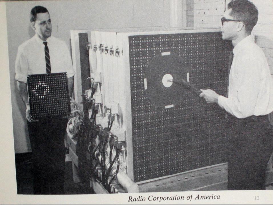
• The earliest type of network to be studied was the perceptron, a single layer of processing elements (Rosenblatt, 1959)

• Data type for inputs, outputs may be binary (0,1) or continuous (real numbers). Weights are generally continuous (typically 0.0-1.0)

• Networks in FEAR use 32-bit floating point numbers for weights• Now that we have a network architecture, we need to specify an

activation function for neurons, an algorithm for recognition mode, and a weight change algorithm for training mode

y

X1

X2

X3

X4

x1

x2

x3

x4

w1

w2

w3

w4

w0

Input vector ->x = [x1...xn]Weight vector ->w = [w0...wn] (w0 is a bias)Output vector ->x = [y1...ym] can have multiple outputs; here this is only one

13

14

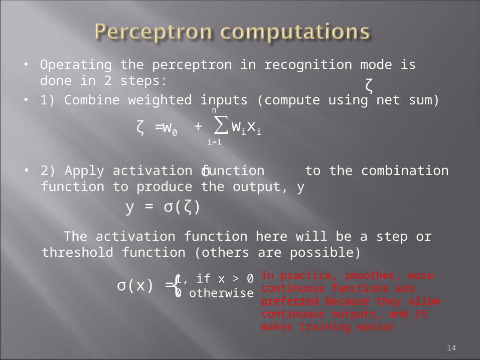
• Operating the perceptron in recognition mode is done in 2 steps: • 1) Combine weighted inputs (compute using net sum)

• 2) Apply activation function to the combination function to produce the output, y

σ

y = σ(ζ)

The activation function here will be a step or threshold function (others are possible)

σ(x) = {1, if x > 00 otherwise

ζ

ζ = w0 + ∑ wixi

n

i=1

In practice, smoother, more continuous functions are preferred because they allow continuous outputs, and it makes training easier

• So the following algorithm may be applied to simulate the output of a

single perceptron. Assume initialised vectors input and weight

For convenience we treat w0 as a (fixed) input at input[0]

netsum = 0 for all i netsum = netsum + input [i] * weight [i] endoutput = activation (netsum)

•With a random set of weights, the perceptron will do a poor job of approximating the function we want. There will be an ideal set of weights that makes it approximate the required function well

•We find those weights by repeatedly clamping the input and output of the perceptron to a known good example pair, then somehow changing the weights to get closer to that mapping. This is supervised learning.

16

• One way of doing this is using the delta rule to optimise the weights incrementally as good training pairs are applied

• The delta rule works on the principles that

- each weight contributes to the output by a variable amount

- The scale of this contribution depends on the input

- The error of the output can be assigned to (blamed on) the weights

• At each example pair, we compare the output of the perceptron y with the ideal output t which gives a relative error E. This is computed by an error function, which is commonly least mean square (LMS) E = ½ (t - y)2

• Then adjust each weight so that the actual output will be slightly closer to the ideal (lower LMS) next time

• If the error function is well-behaved (descends monotonically as we get closer to the ideal perceptron function) we can use this to learn

17

• The delta rule

• Algorithm to apply delta rule. The objective function is a test which determines the overall quality of output (eg total weight adjustment > some threshold)

∂E∆wi = -η∂wi

= ηx1(t-y), where η is a small learning rate

initialise weights randomlywhile (objective function is unsatisfied)

for each sample pairsimulate the perceptronif result is invalid //eg E > some small value for all inputs i

delta = desired - outputweight[i] += eta * delta * input[i]

end for end if

end forend while

• But there is an entire family of patterns which perceptrons cannot learn at all

• In 1969, Minsky & Papert published an influential book in which they proved mathematically that a perceptron cannot learn functions which involve patterns that are linearly seperable eg XOR

• In essence, the argument from these classical AI supporters was that if a function as simple as XOR could not be learned, neural networks were not worth persuing

• The book was very influential, and for a decade, funding for neural net projects all but evaporated

• With an extra (hidden) layer, a neural network could handle such functions – but then there would be no way of computing an error term for the weights of the hidden layer, so the network could not be made to learn

• That is, there was no solution to the credit assignment problem

19

• Minsky, M. & Papert, S, Perceptrons, An Introduction to

Computational Geometry. Cambridge: MIT Press, 1969

• Rosenblatt, F. Principles of Neurodynamics. Spartan Books, 1958

• Simon, H. "Why should machines learn?", in Machine Learning: An Artificial Intelligence Approach, R. S. Michalski, J. G. Carbonell and T. M. Mitchell, Editors 1983, Berlin: Springer-Verlag pp. 25-37. 1983.