ç½ã®Ý ½ M ÖÖ®Ä¦ Modeling Local Scaling Proper for Mul ...

www.vadosezonejournal.org · Vol. 7, No. 2, May 2008 525

T surface soil proper-

ties and estimating soil properties has been signifi cantly

advanced by developments of various types of new space-borne,

airborne, and ground-based sensor technologies. In some areas,

however, due to time and cost constraints, mapping techniques

with point-based fi eld observation and measurement is still com-

monly used. Recently, a suffi cient amount of high-precision data

have become available in mapping properties of soils; for example,

hyperspectral and multispectral remote sensing images with mul-

tiple spatial resolutions are available for mapping soil properties

including humidity, surface roughness, surface crusting, and water

storage (Sullivan et al., 2005). To investigate the scale dependence

of these types of estimation often requires multiple-resolution

images. Representation of such images at multiple scales can be

eff ective for information extraction and map processing. Digital

maps and digital map processing techniques such as geographic

information systems (GIS) and remote sensing image processing

systems have made this possible not only for visualization pur-

poses for maps of various forms and at multiple scales but also for

quantitative digital image processing to analyze data and extract

new information. For example, fusing images with high frequency

but low spatial resolution and images with low frequency but

high spatial resolution to generate new images with both high

frequency and high spatial resolution involves downscaling image

processing. Image fi ltering techniques, commonly used for digital

image processing, enhance some features of interest and reduce

the infl uences of other features considered as noise. For example,

for the purpose of estimation of soil properties, high-frequency

variability of the data caused by local features may be considered

noise that must be removed from the estimation; however, if the

purpose of image processing is to detect anomalies caused by

special features such as water contamination, soil erosion, surface

crusting, and surface roughness, then the high-frequency variabil-

ity of the images must be retained. Th e method introduced here

is useful for mapping these types of properties by separating the

background values with local singularity removed for estimation

of soil properties from anomalous values showing local singularity

for detection of local variability of soil properties.

Th e development of fractal and multifractal theory has pro-

vided the means for describing the regularity of change of spatial

patterns as map scale changes (Mandelbrot, 1972, 1974; Feder,

1988). Th e scale-invariant property (scaling) has not only been

observed from many types of map patterns but also proved to be

useful for characterizing the variability refl ected in a map. Several

multifractal models have been used in geoscience to analyze maps

Modeling Local Scaling Proper esfor Mul scale MappingQiuming Cheng*

State Key Laboratory of Geological Processes and Mineral Resources, China Univ. of Geosciences, Wuhan 430074, Beijing 100083, China; and Dep. of Earth and Space Science and Engineering and Dep. of Geography, York Univ., 4700 Keele St., Toronto, ON M3J 1P3, Canada. Received 13 Feb. 2007. *Corresponding author ([email protected]).

Vadose Zone J. 7:525–532doi:10.2136/vzj2007.0034

© Soil Science Society of America677 S. Segoe Rd. Madison, WI 53711 USA.All rights reserved. No part of this periodical may be reproduced or transmi ed in any form or by any means, electronic or mechanical, including photocopying, recording, or any informa on storage and retrieval system, without permission in wri ng from the publisher.

A : GIS, geographic information systems; IDW, inverse distance weighting.

S S

: M M

Mapping surface soil proper es and es ma ng soil parameters with mul resolu on data has been signifi cantly advanced by newly developed mul scale mapping technologies, which incorporate the concept and models of scaling analysis in data processing. This study was conducted to develop a new mul scale mapping technique on the basis of a power-law model characterizing local singularity of exploratory data for mapping surface soil proper es. A fi eld with singularity due to self-organiza on or self-similarity proper es of the underlying processes can be modeled by mul -fractal models. These types of data may not have the sta s cal sta onary property required by ordinary geosta s cal mapping techniques. The new mapping technique u lizes a scaling property for data interpola on and for downscaling image processing. The inputs, either point data or an image, can be separated into a nonsingular background compo-nent for es ma on purposes and an anomalous component of singularity for mul scale high-pass fi ltering purposes. When used for the purpose of data interpola on, this new method assigns weights for data interpola on by taking into account not only the distance between neighborhood points but also local structures and singularity of the fi eld. The results of applica on of the method to a data set of geochemical concentra on values of Ag from 1172 lake sediments in the Gowganda area of Ontario, Canada, have delineated favorable target areas with strong singularity of Ag concen-tra ons caused by mineraliza on in lake sediments.


or patterns observed on the surface or near the surface of the

Earth or remotely sensed from space (Frisch and Parisi, 1985;

Grassberger, 1983; Hentschel and Procaccia, 1983; Badii and

Politi, 1984, 1985; Halsey et al., 1986; Schertzer and Lovejoy,

1987; Evertsz and Mandelbrot, 1992; Agterberg, 1995, 2005;

Cheng et al., 1994; Cheng, 2007b).

Mapping a feature of interest of an area from point observa-

tion data often involves data interpolation to assign values at the

locations where no measurements are being made. Th e assump-

tion taken for most data interpolation methods is that the values

at known locations are associated with the values at the unknown

locations where the values must be interpolated. Th e association

between the values at diff erent locations is usually related to the

distance between the locations. Th ere have been a number of tech-

niques developed under this assumption for data interpolation.

Th ree common interpolation techniques have been imple-

mented in ArcGIS software (ESRI, 2000), called the spline

method, inverse distance weighting, and kriging. Th e spline

method fi ts a surface to point data with a predetermined spline

function with a certain degree of smoothness, and assumes that

the values for known and unknown locations follow the same

mathematical model and thus can be fi tted with the same type of

function. Th e main advantage of the spline method is the ability to

generate deterministic surfaces from only a few sample points. Th e

main disadvantage of this method is that the spline method applies a

predetermined function that may not fi t the real shape of the data.

Inverse distance weighting (IDW) is a moving-average

technique based on the assumption that the values of the neigh-

boring observations contribute more to the interpolated values

than the values of distant observations. Th e infl uence of the data

at a known point on the interpolation is inversely related to the

distance between the known location and the unknown loca-

tion where values must be estimated. Th e inverse distance decay

rate is determined by a predetermined function parameter. Th e

advantage of the IDW method is that it is intuitive and imple-

mentation is straightforward. Its main disadvantage is related to

the determination of the weights based only on the location and

ignoring the variance of the property of the values themselves.

Kriging is a more sophisticated method that assigns weights

for the location of points by taking into account not only the

distance between the known and unknown locations but also

the spatial association of the values, which is characterized by a

semivariogram function. Kriging is a core subject in the fi eld of

geostatistics, a discipline primarily dedicated to mapping with

spatial statistical and stochastic models. Kriging has long been

applied in the geosciences for data estimation and simulation.

Th e semivariogram is a function measuring the spatial variance

between values at locations separated by a distance (Journel

and Huijbregts, 1978). Th e semivariogram has also been used

for characterizing the structural property of a landscape. As a

second-order moment statistic, the semivariogram requires the

data to have an intrinsic stationary property. Assuming that the

data come from a random process with a constant mean, and

a semivariogram that only depends on the distance and direc-

tion separating any two locations independently, one can fi t a

semivariogram with a mathematical model that can be used as a

global model for assigning associations to any two locations. Th is

is needed to form the normal equations from which the weights

can be obtained for those locations involved for moving averaging

in kriging. Th e major advantage of kriging in comparison with

IDW is estimating weights for locations based not only on the

distance between separated locations but also on the global semi-

variogram model fi tted to the data. One of the main drawbacks

of this method, however, is that it requires data with a stationary

property. Th e stationarity condition may not be met by most

exploratory data with anomalies and extreme values.

A common drawback of the moving average methods,

including IDW and kriging, is that these methods do not take

into account the local properties of the data. Th e method intro-

duced here attempts to overcome the preceding drawbacks by

incorporating local singularity into the basic model of moving

averaging. A power-law model is established for quantifi cation of

local singularity. According to this method, the weights for the

moving average are assigned on the basis of the local scaling prop-

erty of the data. Th e application of this method is demonstrated

using a data set of geochemical element concentration values in

lake sediment samples from the Gowganda area of northeastern

Ontario. Similar applications can be used to map surface soil

properties such as surface crusting, roughness, erosion, and soil

moisture contents.

Materials and MethodsStudy Area and Material Descrip ons

Th e study area is located in the Gowganda–Cobalt area of

northeastern Ontario and is mainly underlain by the Proterozoic

rocks of the Huronian Supergroup (Fig. 1). Th e Huronian rocks

in the area are composed of the Lorrain Formation (quartz sand-

stone, minor conglomerate, and siltstone) and the Gowganda

Formation (mostly diamictite and argillite). Archean-aged supra-

crustal rocks composed of intercalated felsic to mafi c metavolcanic

fl ows with minor ultramafi c to mafi c rocks underlie approxi-

mately 8% of the study area. Felsic intrusive rocks with variable

composition cover approximately 12% of the area (Hamilton,

1997). Diabase intrusions as sills and steeply dipping dikes and

plugs, known as the Nipissing diabase, are quite abundant and

intrude the Archean basement and most of the Huronian rocks.

Approximately 50% of the study area is covered by exposed bed-

rock or relatively thin overburden. Th e Quaternary geology of

the area is mostly characterized by ice-contact stratifi ed drift with

associated sandy glaciofl uvial deposits. Th e dominant ice fl ow is

believed to be an older southwest fl ow superimposed by a younger

south–southeast fl ow (Hamilton, 1997; Panahi et al., 2003).

The Silver Deposits

The Ag sulpharsenide vein deposits in the Cobalt and

Gowganda areas of northeastern Ontario occur along the north

and northeastern margins of the Cobalt Embayment. Th e vein

systems are generally fault controlled, with mineralization occur-

ring adjacent to or within the Nipissing diabase sills, in close

proximity to the Huronian–Archean unconformity (Andrews et

al., 1986). Th e chemistry of the veins indicate Ag, As, Co, Pb,

and rare earth elements among the components introduced with

the hydrothermal fl uids.

Lake Sediment Data

A total of 1172 lake sediment samples were collected from

an area of 2700 km2 by the Ontario Geological Survey in 1997


(Hamilton, 1997), providing a relatively uniform coverage and

regular distribution. To avoid edge eff ects, a smaller area with 925

samples was chosen as the actual area for mapping. Th e sample

locations are shown in Fig. 2. Lake sediment samples were ana-

lyzed by instrumental neutron activation analysis for Au, As, Na,

and Br and by inductively coupled plasma–mass spectrometry

for another 51 elements. Quality control procedures and reports

are found in Hamilton (1997). Th is data set was used by Panahi

et al. (2003) for mapping the mineral potential for Ag and Au

in the area.

Spa al Associa ons, Sta onarity, and Singularity

To discuss spatial association vs. singularity of map values,

we will fi rst introduce several notations and concepts of point

location, point data, pixel, and pixel value. In the GIS context,

a point is represented as a location with two coordinates in

vector format or as a pixel in raster format. Points have no size

but pixels do. Raster maps are built up with pixels and the pixel

size determines the spatial resolution of the map. Th e conver-

sion from point data (vector data) to pixel value (raster data) is

an upscaling process. Assigning values to pixels from point data

often involves data interpolation. How reasonable the estimated

values are for the pixel depends on the complexity of the pixel

values and how many point data can be used to calculate the

pixel values. Diff erentiating these two types of information is

helpful for understanding the concepts of spatial association and

singularity. Th e former is usually calculated directly from the

point data using the distance between sample locations, whereas

the latter is calculated from sets of pixels (or other shapes of

windows) with multiple sizes. Denote the value at point loca-

tion x as Z(x) and the value of a pixel of size ε centered at

location x as μ(x, ε). Th e distance between two points x and y or between pixels centered at x and y can be denoted as ||x − y||.

Th e unit of the distance can be a metric unit or pixels. Th ese

notations help us to discuss the indices of spatial association

and local singularity.

Spa al Associa on

Th e spatial association involved in data interpolation often

represents a type of statistical dependency of values at separate

locations. If the value at a location is considered to be a realization

of a so-called regionalized random variable, the spatial association

or variability can be measured by means of a semivariogram, which

can be expressed as follows (Journel and Huijbregts, 1978):

( ) ( ) ( )[ ]22 ,x Z x Z xγ = − +h h [1]

where γ(x, h) is a function of vector distance h separating

locations x and x + h, and < > is the expectation. Th e semivar-

iogram measures the symmetrical variability between Z(x) and

Z(x + h). Under an assumption of second-order stationarity,

the semivariogram Eq. [1] becomes a function of h indepen-

dent of location x. Th is strong assumption of the regionalized

random variable is generally required in kriging. Th e function

Eq. [1] has been commonly used for structural analysis and for

interpolation in geostatistics (Journel and Huijbregts, 1978).

It has also been applied for texture analysis in image process-

ing (Herzfeld, 1993; Herzfeld and Higginson, 1996; Atkinson

and Lewis, 2000).

F . 1. Simplifi ed geology of the Gowganda area.

F . 2. Loca ons of 925 lake sediment samples from the Gowganda area (data from Hamilton, 1997).


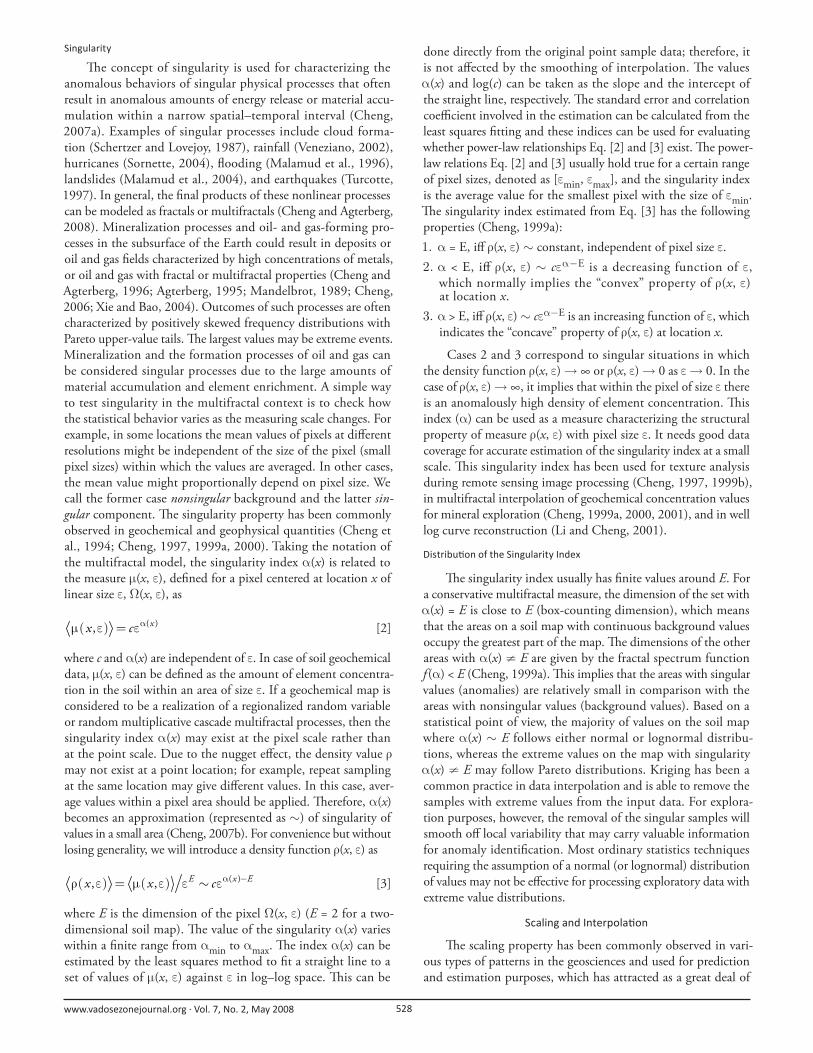
Singularity

Th e concept of singularity is used for characterizing the

anomalous behaviors of singular physical processes that often

result in anomalous amounts of energy release or material accu-

mulation within a narrow spatial–temporal interval (Cheng,

2007a). Examples of singular processes include cloud forma-

tion (Schertzer and Lovejoy, 1987), rainfall (Veneziano, 2002),

hurricanes (Sornette, 2004), fl ooding (Malamud et al., 1996),

landslides (Malamud et al., 2004), and earthquakes (Turcotte,

1997). In general, the fi nal products of these nonlinear processes

can be modeled as fractals or multifractals (Cheng and Agterberg,

2008). Mineralization processes and oil- and gas-forming pro-

cesses in the subsurface of the Earth could result in deposits or

oil and gas fi elds characterized by high concentrations of metals,

or oil and gas with fractal or multifractal properties (Cheng and

Agterberg, 1996; Agterberg, 1995; Mandelbrot, 1989; Cheng,

2006; Xie and Bao, 2004). Outcomes of such processes are often

characterized by positively skewed frequency distributions with

Pareto upper-value tails. Th e largest values may be extreme events.

Mineralization and the formation processes of oil and gas can

be considered singular processes due to the large amounts of

material accumulation and element enrichment. A simple way

to test singularity in the multifractal context is to check how

the statistical behavior varies as the measuring scale changes. For

example, in some locations the mean values of pixels at diff erent

resolutions might be independent of the size of the pixel (small

pixel sizes) within which the values are averaged. In other cases,

the mean value might proportionally depend on pixel size. We

call the former case nonsingular background and the latter sin-gular component. Th e singularity property has been commonly

observed in geochemical and geophysical quantities (Cheng et

al., 1994; Cheng, 1997, 1999a, 2000). Taking the notation of

the multifractal model, the singularity index α(x) is related to

the measure μ(x, ε), defi ned for a pixel centered at location x of

linear size ε, Ω(x, ε), as

( ) ( ), xx c αμ ε = ε [2]

where c and α(x) are independent of ε. In case of soil geochemical

data, μ(x, ε) can be defi ned as the amount of element concentra-

tion in the soil within an area of size ε. If a geochemical map is

considered to be a realization of a regionalized random variable

or random multiplicative cascade multifractal processes, then the

singularity index α(x) may exist at the pixel scale rather than

at the point scale. Due to the nugget eff ect, the density value ρ

may not exist at a point location; for example, repeat sampling

at the same location may give diff erent values. In this case, aver-

age values within a pixel area should be applied. Th erefore, α(x)

becomes an approximation (represented as ∼) of singularity of

values in a small area (Cheng, 2007b). For convenience but without

losing generality, we will introduce a density function ρ(x, ε) as

( ) ( ) ( ), , E x Ex x c α −ρ ε = μ ε ε ∼ ε [3]

where E is the dimension of the pixel Ω(x, ε) (E = 2 for a two-

dimensional soil map). Th e value of the singularity α(x) varies

within a fi nite range from αmin to αmax. Th e index α(x) can be

estimated by the least squares method to fi t a straight line to a

set of values of μ(x, ε) against ε in log–log space. Th is can be

done directly from the original point sample data; therefore, it

is not aff ected by the smoothing of interpolation. Th e values

α(x) and log(c) can be taken as the slope and the intercept of

the straight line, respectively. Th e standard error and correlation

coeffi cient involved in the estimation can be calculated from the

least squares fi tting and these indices can be used for evaluating

whether power-law relationships Eq. [2] and [3] exist. Th e power-

law relations Eq. [2] and [3] usually hold true for a certain range

of pixel sizes, denoted as [εmin, εmax], and the singularity index

is the average value for the smallest pixel with the size of εmin.

Th e singularity index estimated from Eq. [3] has the following

properties (Cheng, 1999a):

α1. = E, iff ρ(x, ε) ∼ constant, independent of pixel size ε.α2. < E, iff ρ(x, ε) ∼ cεα−E is a decreasing function of ε,

which normally implies the “convex” property of ρ(x, ε) at location x.

α3. > E, iff ρ(x, ε) ∼ cεα−E is an increasing function of ε, which

indicates the “concave” property of ρ(x, ε) at location x.

Cases 2 and 3 correspond to singular situations in which

the density function ρ(x, ε) → ∞ or ρ(x, ε) → 0 as ε → 0. In the

case of ρ(x, ε) → ∞, it implies that within the pixel of size ε there

is an anomalously high density of element concentration. Th is

index (α) can be used as a measure characterizing the structural

property of measure ρ(x, ε) with pixel size ε. It needs good data

coverage for accurate estimation of the singularity index at a small

scale. Th is singularity index has been used for texture analysis

during remote sensing image processing (Cheng, 1997, 1999b),

in multifractal interpolation of geochemical concentration values

for mineral exploration (Cheng, 1999a, 2000, 2001), and in well

log curve reconstruction (Li and Cheng, 2001).

Distribu on of the Singularity Index

Th e singularity index usually has fi nite values around E. For

a conservative multifractal measure, the dimension of the set with

α(x) = E is close to E (box-counting dimension), which means

that the areas on a soil map with continuous background values

occupy the greatest part of the map. Th e dimensions of the other

areas with α(x) ≠ E are given by the fractal spectrum function

f (α) < E (Cheng, 1999a). Th is implies that the areas with singular

values (anomalies) are relatively small in comparison with the

areas with nonsingular values (background values). Based on a

statistical point of view, the majority of values on the soil map

where α(x) ∼ E follows either normal or lognormal distribu-

tions, whereas the extreme values on the map with singularity

α(x) ≠ E may follow Pareto distributions. Kriging has been a

common practice in data interpolation and is able to remove the

samples with extreme values from the input data. For explora-

tion purposes, however, the removal of the singular samples will

smooth off local variability that may carry valuable information

for anomaly identifi cation. Most ordinary statistics techniques

requiring the assumption of a normal (or lognormal) distribution

of values may not be eff ective for processing exploratory data with

extreme value distributions.

Scaling and Interpola on

Th e scaling property has been commonly observed in vari-

ous types of patterns in the geosciences and used for prediction

and estimation purposes, which has attracted as a great deal of


attention. A statistical prop-

erty derived at one scale may

be used to estimate the prop-

erty at another scale (Agterberg,

2005). A data interpolation

process that estimates values

for small pixels without obser-

vation of the values available in

surrounding locations can be

considered a type of downscal-

ing process. How to apply the

scaling property in the process

is obviously of general interest.

Th e multifractal interpolation

method developed by Cheng

(1999a, 2000) for construction

of curves (one-dimensional

problem) and surfaces (two-dimensional problem) on the basis of

point observations provides an example of using the scaling proper-

ties of map data for data interpolation. Here we briefl y introduce

the mathematical model of the method.

Equation [3] shows that the average density function defi ned

in a pixel size ε centered at a given location x follows a power-

law relationship with the scale unit (pixel size ε). Th is relation

shows a simple situation of the isotropic scaling property of pixel

value. In a more complex situation when the scaling is anisotropic,

variable window shapes should be used (Cheng, 2004, 2006).

Here we will only deal with the isotropic scaling case, so squares

for windows are applicable. Th e exponent α(x) − E characterizes

the local singularity of the function—how the value changes as

the scale unit decreases. At the singular location α(x) ≠ E, the

density is dependent on the scale unit. In this case, the constant c becomes a useful quantity independent of pixel size and remains

unchanged when pixel size reduces. Th is value of c (c = μ/εα) can

be considered as the measure of the density ρ(x, ε) in the space of

α(x) dimension; for example, if μ stands for metal weight (g) in an

area of linear size ε (cm), then c has the unit (g/cm)α. It becomes

the ordinary density value in nonsingular locations where α = 2.

Th is decomposition is reasonable from the point of view of the

Lebesgue decomposition theorem, which ensures that any com-

plex measure decomposes into an absolutely continuous measure

and a singular measure (Rudin, 1988). Local singularity can also

be characterized in a time series signal by the wavelet transform

method and is related to the Hölder exponent or Lipschitz expo-

nent (Arneodo et al., 1992, 1995, 1998).

If we choose a given pixel size ε0 in Eq. [3] at which the

value of ρ(x, ε0) is calculated as the average density value of the

pixel, then the value for any smaller pixels with size ε < ε0 can be

determined by ρ(x, ε) = (ε/ε0)α(x)−Eρ(x, ε0). Th is property can

be used for downscaling interpolation. For example, we can fi rst

estimate the average value ρ(x, ε0) at a resolution ε0 from the

known values of points within a large window of maximum size

εmax using the moving average weighting model or kriging:

( ) ( ) ( )0 max

0 0 0( , )

,

i

i ix x

x x x Z x∈Ω ε

ρ ε = λ −∑ [4]

where λ(||xi −x0||) is the weighting factor of location xi, which is

a function of the distance from xi to x0, Σ[λ(||xi −x0||)] = 1. Th e

value of λ can be estimated using inverse distance weighting or

kriging methods, usually based on a global model that can deter-

mine the spatial association of the sample locations. Th erefore,

the value of the center pixel at a fi ner resolution ε (ε < ε0) can

be estimated from

( ) ( ) ( ) ( )0

0 max

( )

0 0 0( , )

,

i

x E

i ix x

x x x Z xα −

∈Ω ερ ε = ε ε λ −∑

[5]

Th e factor 0( )0( / ) x Eα −ε ε modifi es the ordinary average in such a

way that if α(x0) < E, then the new result is increased by a factor 0( )

0( / ) x Eα −ε ε given ε < ε0, whereas if α(x0) > E, then the new

result is reduced by a factor 0( )0( / ) x Eα −ε ε . Th is modifi cation is

reasonable because α(x) < E and α(x) > E correspond to convex

and concave properties, respectively, of surface ρ(x, ε) around

the location x. For small pixel size, the average density value ρ(x,

ε) estimated using Eq. [5] with α(x) < E is greater than the esti-

mated value of ρ(x, ε0) obtained by Eq. [4], whereas the value of

ρ(x, ε) with α(x) > E is smaller than the estimated value of ρ(x, ε0).

Th e model not only involves the spatial association refl ected in

the calculation of weight λ but also incorporates the singularity

characterized by the singularity index α(x). Th e main advantages

of the new model in comparison with other ordinary moving

average methods include the use of scaling properties to estimate

pixel values with multiple resolutions, and values of pixels that are

the function of the local singularity measuring the local structure

of the property of the map. Th is property will be demonstrated

with a case study of the concentration value of Ag in lake sedi-

ment samples. Equations [4] and [5] are illustrated in Fig. 3.

Results and DiscussionBoth the ordinary IDW Eq. [4] and the scaling interpola-

tion method Eq. [5] were applied to map the concentration

value of Ag in lake sediments in the entire study area from the

1172 lake sediment samples (925 in the mapping area). Figure

4 shows the map generated from 1172 Ag values by means

of ordinary IDW with a search distance of 11 km, minimum

number of interpolation points of 12, and an inverse distance

decay rate of 2. Th e resultant map is of pixel size = 1 km (1-km

resolution). Figure 5 illustrates the distribution of α(x) values of

pixels of 1-km size estimated from a set of average values of Ag

calculated in squares of sides ε = 1, 3, 5, 7, 9, and 11 km. For

any given pixel (x) on the map, six squares of consecutive sizes

F . 3. Illustra ons showing the processes of the downscaling interpola on Eq. [5] introduced here and the ordinary moving averaging model Eq. [4]: (A) boxes with variable sizes (1–4) were used to calculate the average values from point data (solid dots), while the box labeled εxε is a smaller pixel for which the aver-age value was es mated using Eq. [5]; (B) a plot showing the rela onship between the average element concentra on values μ(x, ε) and box size ε at a log–log scale (solid dots represent the calculated values and the circle for the value to be es mated from Eq. [5]); and (C) the value es mated from neighbor point data to the center using Eq. [4].


were created and the average values μ(x, ε) of Ag were calculated.

Th en a straight line was fi tted to the log-transformed values

logμ(x, ε) and log(ε). Its slope and intercept were chosen as the

α(x) value and log(c), respectively. Th e values of the correlation

coeffi cients and standard errors involved in the estimation of

the α(x) value are >0.975 and <5%, respectively, for most of

the locations, implying that signifi cant linear relationships exist

between logμ(x, ε) and log(ε). Superimposing the locations of

the known Ag deposits on the distribution of α(x) values has

shown that most Ag deposits are located in the areas with α(x) <

2, which indicates a strong spatial association between the areas

of local singularity and the locations of deposits. In many other

areas, similar relationships were found between local singularity

and locations of mineral deposits of Au, Sn, Cu, Pb, and Zn

(Cheng, 2006, 2007a). Th is type of relationship in a mineral

district is common because the areas with low α(x) values may

indicate the areas with enriched geochemical values due to min-

eralization. Comparing the distribution of Ag values in Fig. 4

and the distribution of α(x) values in Fig. 5, we can see that

the moving average values shown in Fig. 4 highlight the general

trends of the Ag values, which may refl ect the general eff ect of

lithology units and structures favorable for Ag mineralization.

Th e distributions usually show continuous and smooth trends

that can be interpolated by various methods including kriging

and IDW. On the contrary, the anomalous values of α(x) shown

in Fig. 5 are the singular component corresponding to a high-

pass fi ltered component that enhances the details related to the

local anomalies of Ag mineral deposits. Th e latter provides a

new way to delineate local anomalies caused by mineralization

in the fractal space of the α dimension. Th is has been demon-

strated to be eff ectively useful for delineating favorable targeting

areas for further mineral exploration; for example, several areas

in the southern part of the map with strong singularity [α(x) <

2] but without discovered Ag mineral deposits can be treated as

target areas for further exploration. In addition, the following

example shows that the local singularity can be used to further

interpolate the IDW map to form a fi ner resolution map. For

example, an α(x) value map at a fi ner resolution, say 200-m

resolution, can be formed by moving-averaging the map in Fig.

5. Th en according to Eq. [5], with the IDW values in Fig. 4 and

the α(x) value at the 200-m resolution, we can generate new

values for Ag at a fi ner resolution, which provides more detail

as shown in Fig. 6 (compare with Fig. 4). Similar results were

obtained from applying the new data interpolation method to

other elements (results not shown).

ConclusionsTh e scaling interpolation method introduced here can be

used for mapping fi elds and downscaling analysis from point

data or an image with local singularity. Th e processed results

using this method contain two separate components: a nonsingu-

lar background component with singularity eliminated that can

be used for estimation purposes and an anomalous component

with strong singularity that can be used for multiscale high-pass

fi ltering purposes. Compared with the ordinary moving average

methods, this new method considers the distance between neigh-

F . 4. Results obtained using the inverse distance weigh ng (IDW) interpola on method for Ag. Pixel size is 1 km, searching distance is 11 km, and inverse distance decay rate was 2.

F . 5. Distribu on of the singularity index α value obtained using Eq. [2] for Ag. Searching scales are 1, 3, 5, 7, 9, and 11 km.


borhood point values and takes local structures and singularity

into account in assigning weights for data interpolation. Th is

example suggests a new direction for improving interpolation

results by utilizing the scaling property quantifi ed by fractal and

multifractal models.

ATh anks are due to Dr. Alireza Ghaff ari for constructive com-

ments. Th is research has been fi nancially supported by a Distinguished Young Researcher Grant (40525009) and a Strategic Research Grant (40638041) awarded by the Natural Science Foundation of China and a High-Tech Research and Development Grant (2006AA06Z115) by the Ministry of Science and Technology of China.

ReferencesAgterberg, F.P. 1995. Multifractal modeling of the sizes and grades of giant and

supergiant deposits. Int. Geol. Rev. 37:1–8.

Agterberg, F.P. 2005. Application of a three-parameter version of the model of

de Wijs in regional geochemistry. p. 291–296. In Q. Cheng and G.F. Bon-

ham-Carter (ed.) GIS and spatial analysis, Proc. IAMG2005, Toronto. Int.

Assoc. Mathmatical Geol., Kingston, ON, Canada.

Andrews, A.J., L. Owsiacki, R. Kerrich, and D.F. Strong. 1986. Th e silver depos-

its at Cobalt and Gowganda, Ontario: I. Geology, petrology, and whole-

rock geochemistry. Can. J. Earth Sci. 23:1480–1506.

Arneodo, A., F. Argoul, E. Bacry, J. Elezgaray, E. Freysz, G. Grasseau, J.F. Muzy,

and B. Pouligny. 1992. Wavelet transform of fractals. p. 287–352. In Y.

Meyer (ed.) Wavelets and applications: Proc. Int. Conf., Marseille, France.

May 1989. Springer-Verlag, Paris.

Arneodo, A., B. Audit, E. Bacry, S. Manneville, J.F. Muzy, and S.G. Roux. 1998.

Th ermodynamics of fractal signals based on wavelet analysis: Applica-

tion to fully developed turbulence data and DNA sequences. Physica A

254:24–45.

Arneodo, A., E. Bacry, and J.F. Muzy. 1995. Th e thermodynamics of fractals

revisited with wavelets. Physica A 213:232–275.

Atkinson, P.M., and P. Lewis. 2000. Geostatistical classifi cation for remote sens-

ing: An introduction. Comput. Geosci. 26:361–371.

Badii, R., and A. Politi. 1984. Hausdorff dimension and uniformity of strange

attractors. Phys. Rev. Lett. 52:1661–1664.

Badii, R., and A. Politi. 1985. Statistical description of chaotic attractors: Th e

dimension function. J. Stat. Phys. 40:725–750.

Cheng, Q. 1997. Multifractal modeling and lacunarity analysis. Math. Geol.

29:919–932.

Cheng, Q. 1999a. Multifractal interpolation. p. 245–250. In S.J. Lippard et

al. (ed.) Proc. Annu. Conf. Int. Assoc. for Mathematical Geol., Trond-

heim, Norway. 6–11 Aug. 1999. Vol. 1. Norw. Univ. of Sci. and Technol.,

Trondheim.

Cheng, Q. 1999b. Multifractality and spatial statistics. Comput. Geosci.

25:949–961.

Cheng, Q. 2000. Interpolation by means of multiftractal, kriging and moving

average techniques. In GeoCanada 2000, Proc. GAC/MAC Meeting, Cal-

gary, AB, Canada [CD-ROM]. 29 May–2 June 2000. Geol. Assoc. Can.,

St. John’s, NF, Canada.

Cheng, Q. 2001. A multifractal and geostatistical method for modeling geo-

chemical map patterns and geochemical anomalies. (In Chinese with Eng-

lish abstract.) J. Earth Sci. 26:161–166.

Cheng, Q. 2004. A new model for quantifying anisotropic scale invariance and

for decomposition of mixing patterns. Math. Geol. 36:345–360.

Cheng, Q. 2006. A new model for incorporating spatial association and singu-

larity in interpolation of exploratory data. p. 1017–1026. In D. Leuangth-

ong and C.V. Deutsch (ed.) Geostatistics Banff 2004. Quantitative Geol.

and Geostat. 14. Springer, New York.

Cheng, Q. 2007a. Mapping singularities with stream sediment geochemical data

for prediction of undiscovered mineral deposits in Gejiu, Yunnan Province,

China. Ore Geol. Rev. 32:314–324.

Cheng, Q. 2007b. Multifractal imaging fi ltering and decomposition methods

in space, Fourier frequency, and eigen domains. Nonlinear Processes Geo-

phys. 14:293–303.

Cheng, Q., and F.P. Agterberg. 1996. Multifractal modeling and spatial statistics.

Math. Geol. 28:1–16.

Cheng, Q., and F.P. Agterberg. 2008. Singularity analysis of ore-mineral and

toxic trace elements in stream sediments. Comput. Geosci. (in press).

Cheng, Q., F.P. Agterberg, and S.B. Ballantyne. 1994. Th e separation of geo-

chemical anomalies from background by fractal methods. J. Explor. Geo-

chem. 51:109–130.

ESRI. 2000. ArcMap, Annual of ArcGIS. ESRI, Redlands, CA.

Evertsz, C.J.G., and B.B. Mandelbrot. 1992. Multifractal measures. p. 922–953.

In H.-O. Peitgen et al. (ed.) Chaos and fractals. Springer, New York.

Feder, J. 1988. Fractals. Plenum Press, New York.

Frisch, U., and G. Parisi. 1985. On the singularity structure of fully developed

turbulence. p. 84–88. In M. Ghil et al. (ed.) Turbulence and predictability

in geophysical fl uid dynamics and climate dynamics. North-Holland, New

York.

Grassberger, P. 1983. Generalized dimensions of strange attractors. Phys. Lett.

A 97:227–230.

Halsey, T.C., M.H. Jensen, L.P. Kadanoff , I. Procaccia, and B.I. Shraiman. 1986.

Fractal measures and their singularities: Th e characterization of strange sets.

Phys. Rev. A 33:1141–1151.

Hamilton, S.M. 1997. A high density lake sediment and water geochemical sur-

vey of 32 geographic townships in the Montreal River headwaters area,

centered on Gowganda area. Open File Rep. 5962. Ontario Geol. Surv.,

Sudbury, ON, Canada.

Hentschel, H.G.E., and I. Procaccia. 1983. Th e infi nite number of generalized

dimensions of fractals and strange attractors. Physica D 8:435–444.

Herzfeld, U.C. 1993. A method for seafl oor classifi cation using directional var-

iogram, demonstrated for data from the western fl ank of the Mid-Atlantic

Ridge. Math. Geol. 25:901–924.

Herzfeld, U.C., and C.A. Higginson. 1996. Automated geostatistical seafl oor

classifi cation: Principles, parameters, feature vectors, and discrimination

criteria. Comput. Geosci. 22:35–52.

Journel, A.G., and Ch.J. Huijbregts. 1978. Mining geostatistics. Academic Press,

New York.

F . 6. A map of Ag created using the scaling interpola on model Eq. [5] with values of the constant c taken from Fig. 4 and singular-ity values es mated for pixels of 200-m size. Triangles represent Ag mineral deposits.


Li, Q., and Q. Cheng. 2001. Fractal correction of well logging curves. J. China

Univ. Geosci. 12:272–275.

Malamud, B.D., D.L. Turcotte, and C.C. Barton. 1996. Th e 1993 Mississippi

River fl ood: A one hundred or a one thousand year event? Environ. Eng.

Geosci. 2:479–486.

Malamud, B.D., D.L. Turcotte, F. Guzzetti, and P. Reichenbach. 2004. Land-

slide inventories and their statistical properties. Earth Surf. Processes Land-

forms 29:687–711.

Mandelbrot, B.B. 1972. Possible refi nement of the lognormal hypothesis con-

cerning the distribution of energy dissipation in intermittent turbulence.

p. 333–351. In M. Rosenblatt and C. Atta (ed.) Statistical models and

turbulence. Lecture Notes in Physics 12. Springer, New York.

Mandelbrot, B.B. 1974. Intermittent turbulence in self-similar cascades: Di-

vergence of high moments and dimension of the carrier. J. Fluid Mech.

62:331–358.

Mandelbrot, B.B. 1989. Multifractal measures, especially for the geophysicist.

Pure Appl. Geophys. 131:5–42.

Panahi, A., Q. Cheng, and G.F. Bonham-Carter. 2003. Modelling lake sediment

geochemical distribution using principal component, indicator kriging

and multifractal power-spectrum analysis: A case study from Gowganda,

Ontario. Geochem. Explor. Environ. Anal. 4:1–12.

Rudin, W. 1988. Real and complex analysis. 3rd ed. Prentice Hall, New York.

Schertzer, D., and S. Lovejoy. 1987. Physical modeling and analysis of rain and

clouds by anisotropic scaling of multiplicative processes. J. Geophys. Res.

92:9693–9714.

Sornette, D. 2004. Critical phenomena in natural sciences: Chaos, fractals, self-

organization, and disorder. 2nd ed. Springer, New York.

Sullivan, D.G., J.N. Shaw, and D. Rickman. 2005. IKONOS imagery to esti-

mate surface soil property variability in two Alabama physiographies. Soil

Sci. Soc. Am. J. 69:1789–1798.

Turcotte, D.L. 1997. Fractals and chaos in geology and geophysics. 2nd ed.

Cambridge Univ. Press, Cambridge, UK.

Veneziano, D. 2002. Multifractality of rainfall and scaling of intensity–dura-

tion–frequency curves. Water Resour. Res. 38:1–12.

Xie, S., and Z. Bao. 2004. Fractal and multifractal properties of geochemical

fi elds. Math. Geol. 36:847–864.

ç½ã®Ý ½ M ÖÖ®Ä¦ Modeling Local Scaling Proper for Mul ...

Documents

Transcript of ç½ã®Ý ½ M ÖÖ®Ä¦ Modeling Local Scaling Proper for Mul ...