6.1 Estimating with Confidence

Inference Statistical confidence Confidence intervals Confidence interval for a population mean Choosing the sample size

1

Introduction Distinguish chance variations from permanent

features of a phenomenon:

◦ Give SAT test to a SRS of 500 Indiana seniors sample mean = 461 What does it say about µ(the mean SAT score of all HS

seniors in Indiana)?

◦ Is 12/20 vs. 8/20 improvements in treatment vs. control group strong enough evidence in favor of a drug?

General principles Methods of formal inference rely on the

assumption that the data come from properly randomized experiment◦ For example an SRS

The field of Statistics gives methods that give correct results a high percentage of times (if repeated many times)

Two most prominent methods are: 1. confidence intervals2. tests of significance (hypothesis testing)

Estimating with confidence

Example 1: ◦Observe 15 plots of corn with yields in

bushels: 138, 139.1, 113, 132.5, 140.7, 109.7, 118.9, 134.8, 109.6,

127.3,115.6, 130.4, 130.2, 111.7, 105.5

◦Sample Mean = 123.8 What can be said about the mean

yield of this variety of corn for the population?

Statistical confidence:

Assume that yield is N(µ, σ) with unknown µ and σ=10 (just assume σ is known)

Then

68-95-99.7% rule: 95% of time sample mean is within 2 standard deviations of population mean◦ 2×2.58 = 5.16 from µ

Thus, 95% of time:

10, , ( , 2.58)

15

X N N Nn

5.16 5.16 X

Put differently: 95% of time

The random interval covers the unknown (but nonrandom) population parameter µ 95% of time.

Our confidence is 95%. We need to be extremely careful when

observing this result.

5.16 5.16 X X

Example 1 (cont):

This particular confidence interval may contain µ or not…

However, such a systematic method gives intervals covering the population mean µ in 95% of cases.

is between 5.16

123.8 5.16

(118.64, 128.96)

X

Confidence Interval

A level C confidence interval for a parameter has two parts:

An interval calculated from the data, which has the form:

estimate ± margin of error

A confidence level C, where C is the probability that the interval will capture the true parameter value in repeated samples. In other words, the confidence level is the success rate for the method.

It does not give us the probability that our parameter is inside the interval.

estimate ± margin of error

The Big Idea: The sampling distribution of tells us how close to µ the sample mean is likely to be. All confidence intervals we construct will have a form similar to this:

Choose an SRS of size n from a population having unknown mean µ and known standard deviation σ. A level C confidence interval for µ is:

The critical value z* is found from the standard Normal distribution.

Confidence Interval for the Mean of a Normal Population

nzx

*

Confidence Interval for a Population Mean

How to find z*:

Example:

C= 95%. Find z* from table A.

See also last row in Table D.

Finding Specific z* Values

We can use a table of z/t values (Table D). For a particular confidence level, C, the appropriate z* value is just above it.

14

Example 2: Tim Kelley weighs himself once a week for

several years. Last month he weighed himself 4 times with an average of 190.5. Examination of Tim’s past data reveals that over relatively short periods of time, his weight measurements are approximately normal with a standard deviation of about 3. Find a 90% confidence interval for his mean weight for last month. Then, find a 99% confidence interval.

Width of CI increases with confidence level:

More confidence wider interval Less confidence narrower interval

Example 2 (cont):

Suppose Tim had only weighed himself once last month and that his one observation was x=190.5 (the same as the mean before). Estimate µ with 90% confidence.

Width of the CI decreases with sample size:

More sample size narrower interval Less sample size wider interval

19

How Confidence Intervals BehaveThe z confidence interval for the mean of a Normal population illustrates several important properties that are shared by all confidence intervals in common use. The user chooses the confidence level and the margin of error follows. We would like high confidence and a small margin of error.

High confidence suggests our method almost always gives correct answers. A small margin of error suggests we have pinned down the parameter

precisely.

The margin of error for the z confidence interval is:

To decrease the margin of error we can: Make z* smaller (the same as a lower confidence level C). Get a bigger n! Since n is under the square root sign, we must take

four times as many observations to cut the margin of error in half. Make σ smaller. Usually not possible.

Impact of Sample Size

Sample size n

Sta

ndar

d er

ror ⁄

√n

The spread in the sampling distribution of the mean is a function of the number of individuals per sample.

The larger the sample size, the smaller the standard deviation (spread) of the sample mean distribution.

The spread decreases at a rate equal to √n.

20

Choosing sample size:

To have a desired margin of error

Take sample (at least) of

*m zn

2*zn

m

Choosing the Sample SizeYou may need a certain margin of error (e.g., in drug trials or manufacturing specs). In most cases, we have no control over the population variability (s), but we can choose the number of measurements (n).

The confidence interval for a population mean will have a specified margin of error m when the sample size is:

m z *n

n z *

m

2

Remember, though, that sample size is not always stretchable at will. There are typically costs and constraints associated with large samples. The best approach is to use the smallest sample size that can give you useful results.

22

Example 2 (cont):

Tim wants to have a margin of error of only 2 pounds with 95% confidence. How many times must he weigh himself to achieve this goal?

Some Cautions

The data should be an SRS from the population. The confidence interval and sample size formulas are

not correct for other sampling methods. Inference cannot rescue badly produced data. Confidence intervals are not resistant to outliers. If n is small (<15) and the population is not Normal, the

true confidence level will be different from C.

The standard deviation of the population must be known. We will learn what to do when is unknown in chapter 7.

24

6.2 Tests of Significance

The reasoning of tests of significance Stating hypotheses Test statistics P-values Statistical significance Test for a population mean Two-sided significance tests and confidence intervals

25

Confidence intervals are one of the two most common types of statistical inference. Use a confidence interval when your goal is to estimate a population parameter. The second common type of inference, called tests of significance, has a different goal: to assess evidence in the data about some claim concerning a population.

26

Statistical Inference

A test of significance is a formal procedure for comparing observed data with a claim (also called a hypothesis) whose truth we want to assess. The claim is a statement about a parameter, like the population proportion

p or the population mean µ. We express the results of a significance test in terms of a probability,

called the P-value, that measures how well the data and the claim agree.

27

The Reasoning of Tests of Significance

We can use software to simulate 400 sets of 50 shots each on the assumption that the player is an 80% free-throw shooter.

Assuming that the actual parameter value is p = 0.80, the observed statistic is so unlikely that it gives convincing evidence that the player’s claim is not true.

You can say how strong the evidence against the player’s claim is by giving the probability that he would make as few as 32 out of 50 free throws if he really makes 80% in the long run.

Suppose a basketball player claimed to be an 80% free-throw shooter. To test this claim, we have him attempt 50 free throws. He makes 32 of them. His sample proportion of made shots is 32/50 = 0.64.

What can we conclude about the claim based on this sample data?

Examples for hypothesis testing:

1. Are Tim Kelly’s weight measurements compatible with the claim that his true mean weight is 187 pounds?

2. In a random sample of 100 light bulbs, 7 are found defective. Is this compatible with the manufacturer’s claim of only 5% of the light bulbs produced are defective?

Example 1: Follow the Tim Kelly Example

What are we in favor of or against? How do we stat this in terms of an appropriate

hypothesis?

Stating Hypotheses

The hypothesis is a statement about the parameters in a population or model – not about the data at hand.◦ We usually have the data and can answer questions directly

about it.

The results of a test are expressed in terms of a probability that measures how well the data and the hypothesis agree.◦ This is similar to confidence but altogether different as well.

In hypothesis testing, we need to state 2 hypotheses:◦ The null hypothesis: H0

◦ The alternative hypothesis: Ha

Null hypothesis: The null hypothesis is the claim which is initially

favored or believed to be true. Often default or uninteresting situation of “no effect” or “no difference”.

THEN, we usually need to determine if there is strong enough evidence against it.

The test of significance is designed to assess the strength of the evidence against the null hypothesis.

Alternative hypothesis:

The alternative hypothesis is the claim that we “hope” or “suspect” something else is true instead of H0.

Sometimes it is easier to begin with the alternative hypothesis Ha and then set up H0 as the statement that the hoped-for effect is not present.

Example 1 cont. (interpretation):

H0: μ = 187

In words: true weight is 187 pounds.

Ha: μ > 187

In words: He weighs more than 187 pounds.

A so-called one-sided alternative Ha.

(Looking for a departure in one direction.)

Example 1 cont. (other possible settings):

H0: μ = 187 vs. Ha: μ <187Suspect the weight is lower. One-sided Ha.

H0: μ = 187 vs. Ha: μ >187Suspect the weight is higher. One-sided Ha. H0: μ =187 vs. Ha: μ ≠187Suspect weight is different. Two-sided Ha.

Note: you must decide on the setting, based on general knowledge, before you see the data or other measurements.

More Examples Translate each of the following research

questions into appropriate hypotheses.

Census Bureau data show that the mean household income in the area served by a shopping mall is $62,500 per year. A market research firm questions shoppers at the mall to find out whether the mean household income of mall shoppers is higher than that of the general population.

Last year, your company’s service technicians took an average

of 2.6 hours to respond to trouble calls from business customers who had purchased service contracts. Do this year’s data show a different average response time?

Example 1 (cont):

Tim Kelley has a driver’s license that gives his weight as 187 pounds. Recall that last month’s mean weight was 190.5, with a sample size of 4. Also the population standard deviation is 3. What is the probability of observing a sample mean of 190.5 or larger when the true population mean is 187?

P-value… the probability, computed assuming that H0 is

true, that the test statistics would take as extreme or more extreme values as the one actually observed.

◦ Example 1 (Tim Kelley): p-value =

This is the P-value of the test (or of the data, given the testing procedure). If it is small, it serves as evidence against H0.

Need to know the distribution of the test statistics under H0 to calculate P-value.

More about P-value…

When the P-Value is small, there are 2 choices:◦ 1—The null hypothesis is true and our observed effect is

extremely rare!OR more likely…◦ 2—The null hypothesis is false and our data is

telling us this by the small P-value! So…

Significance Level We need a cut-off point (decisive value) that we

can compare our P-value to and draw a conclusion or make a decision.◦ In other words, how much evidence do we need to reject

H0 ?

This cut-off point is the significance level. It is announced in advance and serves as a standard on how much evidence against H0 we need to reject H0. Usually denoted α.

Typical values of α: 0.05, 0.01.◦ If not stated otherwise, assume α=0.05.

40

There is no ironclad rule for how small a P-value should be in order to reject H0—it’s a matter of judgment and depends on the specific circumstances. But we can compare the P-value with a fixed value that we regard as decisive, called the significance level. We write it as , the Greek letter alpha. When our P-value is less than the chosen , we say that the result is statistically significant.

If the P-value is smaller than , we say that the data are statistically significant at level . The quantity is called the significance level or the level of significance.

When we use a fixed level of significance to draw a conclusion in a significance test,

P-value < → reject H0 → conclude Ha (in context)

P-value ≥ → fail to reject H0 → cannot conclude Ha (in context)

Statistical Significance

The conclusion/decision: If the P-value is smaller than a fixed significance level α,

then we reject the null hypothesis (in favor of the alternative).

Otherwise we don’t have enough evidence to reject the null.◦ If we don’t reject the null, do we accept it?

Guidelines:◦ IF p-value < α Reject H0

◦ IF p-value > α Fail to Reject H0

Note: Should always report a P-value with your conclusion and write the conclusion in terms of the problem.◦ Conclusion for Example 1 (Tim Kelley):

42

Four Steps of Tests of Significance

1. State the null and alternative hypotheses.

2. Calculate the value of the test statistic.

3. Find the P-value for the observed data.

4. State a conclusion.

Tests of Significance: Four Steps

We will learn the details of many tests of significance in the following chapters. The proper test statistic is determined by the hypotheses and the data collection design.

43

Tests for a Population Mean

z Test for a Population Mean Decision

Reject H0 when the P-value is smaller than significance level α.

Otherwise: Do not reject.

This rule is valid in other settings, too.

One-sided vs. two-sided

If, based on previous data or experience,we expect “increase”, “more”, “better”, etc. (“decrease”, “less”, “worse”, resp.), then we can use a one sided test.

Otherwise, by default, we use two-sided. Key words: “different”, “departures”, “changed”…

A group of 72 male executives in age group 35-44 has mean systolic blood pressure 126.07. Is this career group’s mean pressure different than that of the general population of males in this age group, which is N(128, 15)?

(α not given?? Assume α = 0.05)

Example 2:

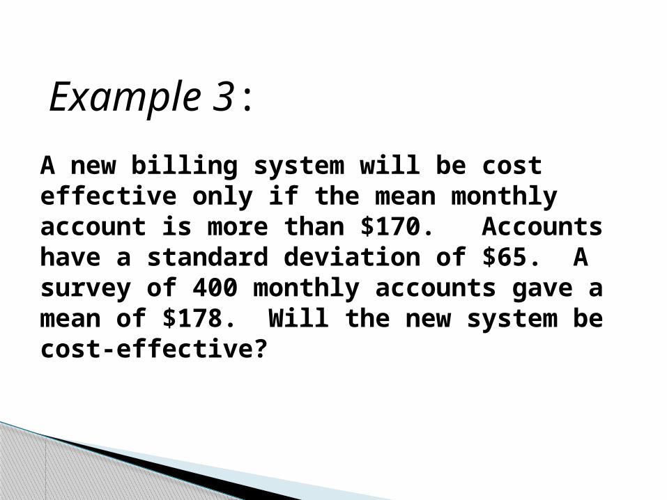
A new billing system will be cost effective only if the mean monthly account is more than $170. Accounts have a standard deviation of $65. A survey of 400 monthly accounts gave a mean of $178. Will the new system be cost-effective?

Example 3:

50

Test StatisticA test of significance is based on a statistic that estimates the parameter that appears in the hypotheses. When H0 is true, we expect the estimate to be near the parameter value specified in H0.

Values of the estimate far from the parameter value specified by H0 give evidence against H0.

A test statistic calculated from the sample data measures how far the data diverge from what we would expect if the null hypothesis H0 were true.

Large values of the statistic show that the data are not consistent with H0.

z estimate - hypothesized value

standard deviation of the estimate

51

More About P-Values

A significance test can be done in a black-and-white manner: We

reject H0 if P < a, and otherwise we do not reject H0.

Reporting the P-value is a better way to summarize a test than

simply stating whether or not H0 is rejected. This is because P quantifies how strong the evidence is against H0. The smaller the

value of P, the greater the evidence. On the other hand, P does not provide specific information about the

true population mean µ. If you desire a likely range of values for the parameter, use a confidence interval.

The p-value is the smallest level α at which the data are significant

Two-sided test and CIs

A level α two-sided significance test rejects H0: µ=µ0 exactly when µ0 falls outside a level 1- α confidence interval for µ.

◦ If µ0 is in the CI fail to reject H0

◦ If µ0 is not in the CI reject H0

◦ NOTE: must have “≠” in Ha!

Example:

An agro-economist examines the cellulose content of a variety of alfalfa hay. Suppose that the cellulose content in the population has a standard deviation of 8 mg. A sample of 15 cuttings has a mean cellulose content of 145 mg. A previous study claimed that the mean cellulose content was 140 mg. The 95% confidence interval is (140.95, 149.05). ◦ Use the confidence interval to determine if the mean

cellulose content is different from 140 mg.

Example (cont):

Now try the test using a test statistic instead of the confidence interval, just for practice. (The result should be the same.)

6.3 Use and Abuse of Tests

Choosing a significance level What statistical significance does not mean Don’t ignore lack of significance Beware of searching for significance

56

Choosing the level of significance

α=0.05 is accepted standard, but… if the conclusion that Ha is true has “costly”

implications, smaller α may be appropriate not always need to make a decision: describing

the evidence by P-value may be enough no sharp border between statistically significant

and insignificant

Statistical vs. practical significance

Statistically significant effect may be small:◦Example (“Executive” blood pressure):

µ0 = 128 σ = 15 n = 1000 obs. sample mean = 127

◦ Z = (127-128)/ (15/sqrt(1000)) = -2.11◦P-value for two sided Ha = 2*0.0174=0.0348

Significant??Stat. significance is not necessarily practical

significance.

Significance vs. practical significance Plot your results and confidence interval, to see if

the effect is worth your attention.

Important effects may have large P-value if sample size too small. Converse also true.

Outliers may produce or destroy statistical significance.

Don’t ignore lack of significance Consider this provocative title from the British Medical Journal: “Absence

of evidence is not evidence of absence.” Having no proof that a particular suspect committed a murder does not

imply that the suspect did not commit the murder.

Indeed, failing to find statistical significance in results means that “the null hypothesis is not rejected.” This is very different from actually accepting the null hypothesis. The sample size, for instance, could be too small to overcome large variability in the population.

When comparing two populations, lack of significance does not imply that the two populations are the same. The populations might be different but have similar statistical properties.

Cautions About Significance Tests

60

Statistical Inference—Not valid for all sets of data!

Statistical Inference, no matter how well done, cannot fix basic flaws in the design◦ Bias due to:

Sampling (like voluntary response, etc) incorrect experimental design Poorly worded questions Etc.

◦ Any other problems we discussed in chapter 3 can affect the validity of the Inference.

Dangers of searching for significance

Example: Take 100 executive rank employees. Measure: blood pressure, height, weight, bone

density, metabolism rate, etc. ◦Test if their blood pressure is different, using α=0.05◦Test if their height is different, using α=0.05◦Test if their weight is different, using α=0.05◦…

If we perform 40 significance tests, how many do we expect to be statistically significant, just by chance?

Dangers of searching for significance

Remember, the significance level controls what we call a “rare” result.

In normal practice, rare results do occur, but rarely!! If α=0.05, then we will rarely (5% of the time) get a rare

result but this is also what we call statistical significance!

In summary, if you are searching for significance by running tests over and over, you will find it! But this is terrible statistics…

We’d much rather have 1 significance test that we are interested in at a single α=0.05!

Cautions (apply both to confidence intervals and tests of significance):

Data: an SRS Formulas for other randomized designs available Haphazard data = unreliable CI Population need not be normal but outliers pose a

threat to validity of conclusions Will learn how to estimate σ in Chapter 7