University of Southampton Research Repository

ePrints Soton

Copyright © and Moral Rights for this thesis are retained by the author and/or other copyright owners. A copy can be downloaded for personal non-commercial research or study, without prior permission or charge. This thesis cannot be reproduced or quoted extensively from without first obtaining permission in writing from the copyright holder/s. The content must not be changed in any way or sold commercially in any format or medium without the formal permission of the copyright holders.

When referring to this work, full bibliographic details including the author, title, awarding institution and date of the thesis must be given e.g.

AUTHOR (year of submission) "Full thesis title", University of Southampton, name of the University School or Department, PhD Thesis, pagination

http://eprints.soton.ac.uk

University of Southampton Faculty of Engineering, Science and Mathematics School of Civil Engineering and the Environment

The role of frictional heating in the development of catastrophic landslides

By

Francesco Cecinato

Thesis for the degree of Doctor of Philosophy

February 2009

ii

Era lo loco ov'a scender la riva

venimmo, alpestro e, per quel che v'er'anco,

tal, ch'ogne vista ne sarebbe schiva.

Qual e` quella ruina che nel fianco

di qua da Trento l'Adice percosse,

o per tremoto o per sostegno manco,

che da cima del monte, onde si mosse,

al piano è sì la roccia discoscesa,

ch'alcuna via darebbe a chi sù fosse;

[The place where to descend the bank we came

Was alpine, and from what was there, moreover

Of such a kind that every eye would shun it

Such as that ruin is which in the flank

Smote, on this side of Trent, the Adige

Either by earthquake or by failing stay

For from the mountain's top, from which it moved,

Unto the plain the cliff is shattered so,

Some path 'twould give to him who was above;]

(Dante Alighieri, The Divine Comedy, Hell, canto XII)

iii

UNIVERSITY OF SOUTHAMPTON

ABSTRACT

FACULTY OF ENGINEERING, SCIENCE & MATHEMATICS SCHOOL OF CIVIL ENGINEERING & THE ENVIRONMENT Doctor of Philosophy THE ROLE OF FRICTIONAL HEATING IN THE DEVELOPMENT OF CATASTROPHIC LANDSLIDES by Francesco Cecinato In this work, a new thermo-mechanical model is developed by improving on an existing one, applicable to large deep seated landslides and rockslides consisting of a coherent mass sliding on a thin clayey layer. The considered time window is that of catastrophic acceleration, starting at incipient failure and ending a few seconds later, when the acquired displacement and velocity are such that the sliding material begins to break up into pieces. The model accounts for temperature rise in the slip zone due to the heat produced by friction, leading to thermoplastic collapse of the soil skeleton and subsequent increase of pore water pressure. This in turn drastically decreases the resistance to motion and allows the overlying mass to move downslope ever more freely. The proposed model is implemented numerically and validated by back-analysing the two well-documented catastrophic landslide case histories of Vajont and Jiufengershan. The model is then employed to carry out a parametric study to systematically investigate the development of catastrophic failure in uniform slopes. It was found that the most influential parameters in promoting catastrophic collapse are (1) the static friction-softening rate a1, (2) the slope inclination β, (3) the soil permeability kw, (4) the dynamic residual friction angle rdφ and (5) the overburden thickness H. The most

dangerous situation is when a1, β and H are very large and kw and rdφ are very low. Of

the above, the ‘thermo-mechanical parameters’ kw and H deserve more attention as they have been introduced by the thermo-mechanical model and are not normally considered in standard stability analyses of uniform slopes. A second parametric study was performed to demonstrate that thermo-mechanical parameters alone can make a difference between a relatively non-catastrophic event and a catastrophic one. Hence, further insight into the design of landslide risk mitigation measures can be gained if, in addition to the standard site investigations, the permeability of the soil is measured and the depth of an existing or expected failure surface is measured or estimated respectively.

iv

Contents

ABSTRACT iii List of figures vii List of tables xii Declaration of authorship xiii Acknowledgements xiv Notation xv

CHAPTER 1. INTRODUCTION 1 1.1. BACKGROUND 1 1.2. AIMS AND OBJECTIVES 2 1.3. STRUCTURE OF THESIS 3

CHAPTER 2. A REVIEW OF LANDSLIDE CASE STUDIES AND MODELLING 5 2.1. SUB-AERIAL LANDSLIDE CASES 5

2.1.1. Classification of sub-aerial slope movements 5 2.1.2. From generic ‘slope movements’ to ‘catastrophic landslides’ 9 2.1.3. Two important sub-cases: Deep-seated and flow-like movements 12 2.1.4. Landslide case studies 13

2.1.4.1. Large masses sliding in a coherent state with long run-out 15 2.1.4.2. Large masses with short run-out 16 2.1.4.3. Large masses achieving a long run-out after evolving into a flow-like phenomenon 17 2.1.4.4. Smaller masses with high destructive potential 18 2.1.4.5. Some catastrophic landslide cases 18

2.2. SUBMARINE LANDSLIDE CASES 23 2.2.1. Classification of submarine landslides 23 2.2.2. Typical environments and causes of submarine landslides 25 2.2.3. Similarities and differences between terrestrial and submarine landslides 27 2.2.4. Data availability and trends in submarine mass wasting phenomena 28

2.2.4.1. Observations from the available literature 28 2.2.4.2. Data collection 31 2.2.4.3. Relevance of submarine landslides to our research 33

2.3. CATASTROPHIC LANDSLIDES. REVIEW OF EXISTING THEORIES 34 2.3.1. Field evidence of frictional heating 35 2.3.2. Some theories on the thermal collapse of landslides 37 2.3.3. The mechanism of thermal pressurisation 39 2.3.4. A comprehensive thermo-poro-mechanical model 41

2.3.4.1. The shearband equations 45 2.3.4.2. The dynamical equation 47 2.3.4.3. The landslide equations 47 2.3.4.4. Vardoulakis’ computational results and discussion 48

CHAPTER 3. THERMO-PLASTICITY IN CLAYS. REVIEW OF EXISTING MODELS 51 3.1. THE NEED FOR THERMOPLASTIC CONSTITUTIVE MODELLING 51 3.2. THE ‘INGREDIENTS’ OF SOIL ELASTO-PLASTICITY 51 3.3. HUECKEL’S CONSTITUTIVE MODEL 52

3.3.1. Thermoelasticity 53 3.3.2. Yield surface 53 3.3.3. Hardening relationship 54 3.3.4. Flow rule 54 3.3.5. Consistency condition and plastic multiplier 55 3.3.6. Loading/unloading and hardening/softening conditions 55 3.3.7. Associative flow rule 58

3.4. LALOUI’S CONSTITUTIVE MODEL 59 3.4.1. Introduction 59 3.4.2. Thermoelasticity 60 3.4.3. Multi-mechanism thermoplasticity 60

3.4.3.1. Isotropic yield mechanism and flow rule 61 3.4.3.2. Deviatoric yield mechanism and flow rule 61

v

3.4.3.3. Thermal dependency of the soil’s friction angle 62 3.4.3.4. Volumetric strain coupling and consistency conditions 64

3.5. OTHER AUTHORS’ CONTRIBUTIONS TO THERMO-MECHANICAL SOIL MODELLING 64 3.5.1. Sultan’s model 65 3.5.2. Robinet’s model 66

3.6. DISCUSSION 67 CHAPTER 4. AN IMPROVED THERMO-MECHANICAL CONSTITUTIVE MODEL 68

4.1. INTRODUCTION 68 4.2. PROBLEM FORMULATION 68 4.3. THERMOELASTICITY 71 4.4. THERMOPLASTICITY 72

4.4.1. Calculation of the plastic multiplier 72 4.4.2. Thermo-elasto-plastic stress-strain rate equations 74 4.4.3. Hardening law and final thermoplastic equations 74

4.5. NUMERICAL INTEGRATION SCHEME 76 4.5.1. Overview of integration algorithms 76

4.5.1.1. Explicit methods 77 4.5.1.2. Implicit methods 78 4.5.1.3. A refined explicit scheme 79

4.5.2. Strain-controlled integration scheme 80 4.5.3. Elasticity domain and yield surface intersection 81 4.5.4. Elasto-plasticity domain 84

4.6. NUMERICAL RESULTS 87 CHAPTER 5. MODIFIED LANDSLIDE MODEL 91

5.1. MODEL ASSUMPTIONS AND OVERVIEW 91 5.2. HEAT EQUATION 93

5.2.1. Material softening law 96 5.2.2. Thermal hardening law defining the stress state 98 5.2.3. Plastic multiplier 100 5.2.4. Final form of heat equation 101

5.3. PORE PRESSURE EQUATION 102 5.3.1. Consolidation coefficient 103 5.3.2. Pressurisation coefficient and thermal volumetric behaviour of clay 105

5.3.2.1. Determination of λm according to Vardoulakis 106 5.3.2.2. Determination of λm consistently with the new constitutive model 110 5.3.2.3. Compressibility coefficient and mean stress 113

5.4. DYNAMICAL EQUATION 115 5.5. NUMERICAL IMPLEMENTATION 118

5.5.1. Discussion on integration methods 118 5.5.2. Discretisation 121 5.5.3. Choice of parameters for the Vajont case study 122

5.5.3.1. Void ratio 122 5.5.3.2. Isothermal preconsolidation stress 123 5.5.3.3. Plastic compressibility 124 5.5.3.4. Thermo-elastic expansion 124 5.5.3.5. Thermal friction sensitivity 124 5.5.3.6. Thermal softening parameter ‘γ’ and resulting values of the pressurisation coefficient 125

5.5.4. Well-posedness of the heat equation 126 5.5.5. Time-step analysis 127 5.5.6. Initial and boundary conditions 129 5.5.7. Numerical results for Vajont 130

5.5.7.1. Vaporisation threshold 130 5.5.7.2. Case of thermal-only friction softening 131 5.5.7.3. Case of ‘full’ friction softening 134 5.5.7.4. Case of absent thermal friction softening 138 5.5.7.5. Discussion on numerical results 140

CHAPTER 6. GENERALISATION TO INFINITE SLOPE GEOMETRY 142 6.1. INFINITE SLOPE ANALYSIS 142

6.1.1. Static analysis to determine incipient failure conditions 142

vi

6.1.2. Dynamic analysis 144 6.1.3. Stress state assumptions 145

6.2. NUMERICAL IMPLEMENTATION 146 6.3. BACK-ANALYSIS OF THE JIUFENGERSHAN SLIDE 147

6.3.1. Overview of the slide 148 6.3.2. Selection of parameters 148 6.3.3. Seismic triggering phase: undrained failure 151 6.3.4. Catastrophic collapse phase 153 6.3.5. Cases of friction-softening soil and thinner shearband 161

CHAPTER 7. PARAMETRIC ANALYSIS TO DETERMINE THE CRITICAL CONDITIONS TO CATASTROPHIC FAILURE 167

7.1. ON THE DEFINITION OF ‘CATASTROPHIC’ SLIDE 167 7.2. CHOICE OF PARAMETERS AND THEIR RANGE 169

7.2.1. Selected parameters 169 7.2.2. Range of selected parameters 170 7.2.3. Parameters that are kept constant 171

7.3. GENERALISATION OF INITIAL CONDITIONS 171 7.4. PARAMETRIC ANALYSIS 174

7.4.1. Factorial vs. Taguchi analysis 174 7.4.2. A general Taguchi analysis 176

7.4.2.1. Level average analysis 178 7.4.2.2. Reliability check 180 7.4.2.3. Discussion of the results 181

7.4.3. A Taguchi analysis focusing on thermo-mechanical effects 184 7.4.3.1. Level average analysis 185 7.4.3.2. Results and discussion 186

7.5. LIMITATIONS OF THE INFINITE SLOPE MODEL 188 CHAPTER 8. CONCLUSIONS AND FUTURE WORK 190

8.1. GENERAL CONCLUSIONS 190 8.2. RECOMMENDATIONS FOR FURTHER RESEARCH 191

APPENDIX 193 REFERENCES 212

vii

List of figures

Figure 1. Residual friction angles from ring shear tests on different soils (Skempton 1985). ..............................................................................................................................14 Figure 2. Overview of the Vajont valley after the disaster. Photo from Schrefler (2005)..........................................................................................................................................19 Figure 3. Historical photo of the location where the village of Longarone once stood, taken shortly after the disaster. Photo from Bojanowski (2007).....................................19 Figure 4. From Shou and Wang (2003). The planar slide of Jiufengershan, occurred in Taiwan in 1999................................................................................................................20 Figure 5. From Thuro et al. (2005). the Goldau landslide in a painting by H. Keller, 1806.................................................................................................................................21 Figure 6. From Yueping (2008). Overview of Qiangjiangping slide, occurred in 2003 in China. ..............................................................................................................................21 Figure 7. From Yueping (2008). Qiangjiangping landslide: (a) Sections of the slope before and after the slide and (b) photo of the slip surface.............................................22 Figure 8. Classification of submarine slides by Prior (1988). ........................................24 Figure 9. Classification of submarine slides by Lee et al. (1988)...................................25 Figure 10. Events that are likely to trigger submarine slides by reducing their safety factor (Locat and Lee, 2000)...........................................................................................25 Figure 11. From Legros, 2002. Relationships between geometrical properties plotted for sub-aerial volcanic and non-volcanic slides, submarine slides and martian slides. (a) Ratio of total fall height/runout vs volume, (b) runout vs volume, (c) fall height vs runout, (d) fall height vs volume, (e) area covered by the landslide deposit vs volume, (f) Author’s legend..........................................................................................................29 Figure 12. Percentages of disintegrative and non-disintegrative submarine landslides (Booth et al., 1991) .........................................................................................................30 Figure 13. Frequency of occurrence of different types of submarine landslides. ...........30 Figure 14. Soil properties deduced from four marine sediment cores (Lykousis et al., 2002) ...............................................................................................................................32 Figure 15. Example of submarine core logs data (Urgeles et al, 2006). .........................33 Figure 16. Frictionite samples from Koefels rockslide: on the left, typical porous pumice-like piece (Erismann and Abele, 2001); on the right, twin-phased pumice as evidence of turbulence in the liquid state of the rock (Erismann, 1979). .......................35 Figure 17. From Erismann and Abele (2001). Glassy frictionite (vein across the picture diagonal) from a secondary sliding surface in Koefels slide. .........................................36 Figure 18. From Lin et al. (2001). Glass matrix with irregular shaped clasts (left) and vescicles (right) within the pseudotachylite found in the slip plane of Jiufengershan landslide. .........................................................................................................................36 Figure 19. From Zhang et al. (2002). Muscovite flakes oriented parallel to shear direction taken from the rupture plane of Sale Mountain Landslide. .............................37 Figure 20. ‘Section 5’ of Vajont landslide and schematic enlargement of the shearband area, where all deformation is concentrated during sliding (after Vardoulakis, 2002a). 43 Figure 21. Scheme of the Mohr-Coulomb constitutive model from Vardoulakis (2002a). Compressive stress is taken negative in this plot. ...........................................................44 Figure 22. Displacement softening data from ring shear tests (Tika and Hutchinson, 1999) and hyperbolic interpolation law (Vardoulakis, 2002a). ......................................44 Figure 23. Velocity softening data from ring shear tests (Tika and Hutchinson, 1999) and hyperbolic interpolation law (Vardoulakis, 2002a)..................................................45

viii

Figure 24. Temperature (a) and excess pore pressure (b) isochrones along the domain thickness as computed by Vardoulakis (2002a)..............................................................48 Figure 25. Computed landslide velocity over time, for the Vajont case (Vardoulakis, 2002a)..............................................................................................................................49 Figure 26. Computed landslide displacement over time, for the Vajont case (Vardoulakis, 2002a).......................................................................................................50 Figure 27. Sample thermo-plastic yield locus in three dimensions, with sample stress-temperature rate vector Δv. .............................................................................................57 Figure 28. Projections of the stress-temperature rate vector Δv (Figure 27) on the deviatoric stress vs. temperature plane and on the deviatoric stress vs. mean effective stress plane. .....................................................................................................................58 Figure 29. Isotropic yield locus (Laloui et al., 2002)......................................................62 Figure 30. Experimental data on the influence of temperature on the friction angle at critical state of some clays (Laloui et al., 2001). ............................................................63 Figure 31. From Marques et al. (2004). Temperature effect on the critical state line for the St-Roch-de-l’Achigan Canadian clay........................................................................64 Figure 32. From Laloui et al., 2005. Coupled yield loci enclosing the thermo-elastic domain in terms of mean isotropic stress (p’), deviatoric stress (q) and temperature (T)..........................................................................................................................................65 Figure 33. From Cui et al. (2000). Yield surface in 3 dimensions. On the temperature (T) vs. isotropic stress (p’) plane, TY represents the newly introduced thermal yield curve, while LY corresponds to Hueckel’s hardening law. ............................................66 Figure 34. Qualitative shape of the thermo-plastic yield locus at critical state, demonstrating temperature dependence of the apparent preconsolidation stress and thermal-friction softening. ..............................................................................................69 Figure 35. Scheme of the Forward Euler method. This is the simplest and least accurate method for the integration of an ODE. To find the next function value (2), the derivative at the start of the interval (1) is used. After Press at al., 1988. .......................................78 Figure 36. Fourth-order Runge-Kutta method. The derivative at point n+1 is calculated from the known value at 1 (filled-in dot) and three trial values at 2,3,4 (open dots). After Press at al., 1988. ............................................................................................................79 Figure 37. Geometry of the yield surface intersection problem. Comparison between isothermal case (dotted lines) and the more complicated case of thermo-mechanical loading (dashed lines): segments σ0B and σ0D represent the total ‘secant’ stress increment, OA and OC the ‘elastic portion’ to be calculated. ........................................82 Figure 38. Numerical simulations with our code of isothermal oedometric compression of a soil element. Loading path in deviatoric plane (p’, q) .............................................89 Figure 39. Numerical simulations with our code of isothermal oedometric compression of a soil element. Loading path in compression plane (ln(p’), e). ..................................89 Figure 40. Numerical simulation of some thermo-mechanical isotropic paths. The dashed line represents isothermal loading (at 20°C), the solid line thermo-mechanical loading where temperature is increased from 20°C to 60°C, the dash-dotted path was obtained by applying a higher temperature rate (a 40°C increase during the first 1/20 of total loading), followed by mechanical loading only......................................................90 Figure 41. Simulation of isothermal loading and combined thermo-mechanical loading compared to experimental data of isothermal isotropic compression at different temperatures (data points from Laloui and Cekerevac, 2003). The black line simulates thermo-mechanical loading until temperature reaches 60 °C, followed by mechanical loading only. It can be seen how the state path moves between the two sets of data corresponding to isothermal compression at the respective temperatures. .....................90

ix

Figure 42. Scheme of the shearband with axis reference system. The out-of-plane direction is y. ...................................................................................................................93 Figure 43. Sample stress state in critical state conditions, ‘locked’ at the peak point of the Modified Cam Clay ellipse. ......................................................................................93 Figure 44. Effective stress paths of material points inside the shearband. .....................99 Figure 45. Experimental results showing the variation of the consolidation coefficient of a saturated clay with temperature (Delage et al., 2000)................................................104 Figure 46. Vardoulakis’ interpolation of experimental data (bottom-right line) and calculations according to the landslide model’s assumptions (over-lying line) for the consolidation coefficient. From Vardoulakis (2002a). .................................................104 Figure 47. Experimentally observed volume changes from isotropic heating tests, at different OCRs, for a kaolin clay (from Laloui and Cekerevac, 2003).........................107 Figure 48. From Baldi et al. (1991). Volumetric response of Boom clay to drained isotropic heating/cooling tests, for different OCRs.......................................................108 Figure 49. From Vardoulakis (2002a). Isotropic thermal volumetric deformation of an over-consolidated ‘Boom clay’ (OCR=12). The experimental data by Sultan (1997) have been interpolated with a bi-linear law by Vardoulakis (2002a). A-B represents the thermoelastic expansion, at B the ‘transition’ or ‘critical’ temperature is reached after which thermoplastic collapse (B-C) follows. CD represents the cooling phase and shows thermoelastic contraction. .............................................................................................108 Figure 50. Data points from Sultan (1997) showing the dependency of the elasto-plastic thermal expansion coefficient (a) and critical temperature (b) on the soil’s OCR; and relative interpolating lines (Vardoulakis 2002a). It can be noticed that, while the data on critical temperature show a clear trend, those regarding the elasto-plastic coefficient are rather scattered. .............................................................................................................109 Figure 51. From Vardoulakis (2002a). Critical failure circle for ‘section 6’ of the Vajont slide. The epicentric angle represents the immersed part of the circular failure surface, and corresponds to the portion α- α1=(37°-11°) in this case. ........................................117 Figure 52. Sample finite difference grid, defining the discretised solution domain for a parabolic PDE. ..............................................................................................................118 Figure 53. From Hoffman (2001). Numerical domain of dependence for explicit methods, for 1-D propagation PDEs. The spatial coordinate is x. ................................120 Figure 54. From Hoffman (2001). Numerical domain of dependence for implicit methods, for 1-D propagation PDEs. The spatial coordinate is x. ................................120 Figure 55. Calculation of pressurisation coefficient λm as a function of temperature, for four different values of the thermal softening parameter γ. .........................................125 Figure 56. Calculation of the sign of coefficient Di for mid-range values of involved parameters (whose typical ranges are listed in the framed box) and temperature ranging between 0 and 1000 °C. ................................................................................................127 Figure 57. Finite difference grid showing the thickness domain of integration. The shearband is a strain localisation zone of thickness d, embedded in an otherwise homogeneous soil layer of total thickness 10d. The soil below the shearband is still, while the soil at the top of the shearband moves at the velocity vd, characteristic of the landslide overburden. ....................................................................................................130 Figure 58. Temperature isochrones within the shearband and its surroundings, for the case of thermal-only friction softening. The shearband area, where strain localisation takes place, is shaded. ...................................................................................................132 Figure 59. Pore pressure isochrones within the shearband and its surroundings, for the case of thermal-only friction softening. The shearband area, where strain localisation takes place, is shaded. ...................................................................................................133

x

Figure 60. Slide velocity profile for the case of thermal-only friction softening. ........133 Figure 61. Slide displacement profile for the case of thermal-only friction softening. 134 Figure 62. Temperature isochrones within the shearband and its surroundings, for the case of full friction softening. The shearband area, where strain localisation takes place, is shaded. .......................................................................................................................136 Figure 63. Pore pressure isochrones within the shearband and its surroundings, for the case of full friction softening. The shearband area, where strain localisation takes place, is shaded. .......................................................................................................................136 Figure 64. slide velocity profile for the case of full friction softening. ........................137 Figure 65. Slide displacement profile for the case of full friction softening. ...............137 Figure 66. Temperature isochrones within the shearband and its surroundings, for the case of displacement and velocity softening only. The shearband area, where strain localisation takes place, is shaded.................................................................................138 Figure 67. Pore pressure isochrones within the shearband and its surroundings, for the case of displacement and velocity softening only. The shearband area, where strain localisation takes place, is shaded.................................................................................139 Figure 68. slide velocity profile for the case of displacement and velocity softening only................................................................................................................................139 Figure 69. Slide displacement profile for the case of displacement and velocity softening only................................................................................................................140 Figure 70. Infinite slope geometry. The shearband (shaded) has negligible thickness compared to that of the overburden, i.e. H»d. The slope inclination with respect to horizontal is β. ...............................................................................................................143 Figure 71. From Chang et al. (2005a). Simulation of the time evolution of shear stress (τ), displacement (d), temperature (T) and pore pressure (Up) for the Jiufengershan slide in the catastrophic case scenario (avalanche regime). The seismic triggering phase, where the increase of pore pressure and temperature is not significant, lasts up to about 50 seconds, after which the drastic build-up of both T and Up determines catastrophic collapse due to rapid vanishing of the shear strength. The vertical dashed line marks the approximate boundary between the two phases............................................................154 Figure 72. Sample stress paths of undrained failure from the initial undisturbed state (I) to the final critical state (F) in the compression plane, for the two cases of (a) initially NC soil and (b) initially OC soil. ..................................................................................155 Figure 73. Temperature isochrones from our calculations to interpret the catastrophic collapse phase of Jiufengershan. ...................................................................................156 Figure 74. Excess pore pressure isochrones from our calculations to interpret the catastrophic collapse phase of Jiufengershan................................................................156 Figure 75. Computed shear stress and excess pore pressure at the shearband mid-plane as a function of time......................................................................................................157 Figure 76. Computed velocity profile to simulate the catastrophic collapse phase of the Jiufengershan slide. .......................................................................................................157 Figure 77. Computed displacement profile to simulate the catastrophic collapse phase of the Jiufengershan slide. .................................................................................................158 Figure 78. Computed velocity and displacement of the Jiufengershan slide, plotted against time for the first 40 seconds of catastrophic collapse. The vertical dashed line marks the reaching of 1km of displacement, roughly corresponding to a velocity of 80 m/s. ................................................................................................................................158 Figure 79. Comparison between our simulations and those of Chang et al. (2005a) of the temperature profile at the shearband mid-plane of the Jiufengershan landslide...........159

xi

Figure 80. Comparison between our simulations and those of Chang et al. (2005a) of the total pore pressure profile at the shearband mid-plane of the Jiufengershan landslide.160 Figure 81. Comparison between our simulations and those of Chang et al. (2005a) of the shear stress profile at the shearband mid-plane of the Jiufengershan landslide............160 Figure 82. Temperature isochrones from our calculations to interpret the catastrophic collapse phase of Jiufengershan, in the case of friction-softening soil. ........................162 Figure 83. Excess pore pressure isochrones from our calculations to interpret the catastrophic collapse phase of Jiufengershan, in the case of friction-softening soil.....162 Figure 84. Computed shear stress and excess pore pressure at the shearband mid-plane as a function of time, in the case of friction-softening soil...........................................163 Figure 85. Computed temperature at the shearband mid-plane as a function of time, in the case of friction-softening soil..................................................................................163 Figure 86. Computed velocity and displacement of the Jiufengershan slide, plotted against time for the first 20 seconds of catastrophic collapse, in the case of friction-softening soil. ................................................................................................................164 Figure 87. Temperature isochrones from our calculations to interpret the catastrophic collapse phase of Jiufengershan, in the case of thinner shearband (d=1mm instead of 1cm). .............................................................................................................................164 Figure 88. Excess pore pressure isochrones from our calculations to interpret the catastrophic collapse phase of Jiufengershan, in the case of thinner shearband (d=1mm instead of 1cm)..............................................................................................................165 Figure 89. Computed shear stress and excess pore pressure at the shearband mid-plane as a function of time, in the case of thinner shearband (d=1mm instead of 1cm). .......165 Figure 90. Computed velocity profile to simulate the catastrophic collapse phase of the Jiufengershan slide, in the case of thinner shearband (d=1mm instead of 1cm). .........166 Figure 91. Preliminary study on the effect of the overburden thickness H on the slide velocity..........................................................................................................................169 Figure 92. Scheme of an infinite slope of inclination β through which water is flowing at inclination αs. An open-end standpipe is represented to highlight the equipotential level relevant to points situated along segment AB...............................................................173

xii

List of tables

Table 1. From Shuzui (2000). Classification method based on the history of landslide movements and the properties of the slip surface. ............................................................9 Table 2. IUGS (1995) landslide velocity classification. .................................................11 Table 3. Selected catastrophic landslide cases................................................................18 Table 4. Material and system parameters chosen to back-analyse the Vajont landslide........................................................................................................................................123 Table 5. Field data of Jiufengershan slide.....................................................................149 Table 6. Choice of parameters for Jiufengershan slide. ................................................150 Table 7. Combinations of parameters for which the excess pore pressure to failure is calculated. .....................................................................................................................153 Table 8. Parameters selected for the parametric study and their levels. .......................174 Table 9. Sample orthogonal array containing the settings for a 3-parameter, 2-level analysis..........................................................................................................................176 Table 10. Orthogonal array for a 7-parameter, 2-level analysis where the levels in three samples columns are shaded with different tones to illustrate the feature of orthogonality between columns...........................................................................................................177 Table 11. Orthogonal array for the infinite slide parametric analysis..........................182 Table 12. Response table of our 13-parameter landslide model Taguchi analysis. ......183 Table 13. Parameter settings for the confirmation run of our general Taguchi analysis........................................................................................................................................183 Table 14. Parameter levels for the 4-parameter Taguchi analysis. ...............................185 Table 15. Orthogonal array for the infinite slide 4-parameter analysis. .......................186 Table 16. Response of the level average analysis. ........................................................186

xiii

Declaration of authorship

I, FRANCESCO CECINATO, declare that the thesis entitled THE ROLE OF FRICTIONAL HEATING IN THE DEVELOPMENT OF CATASTROPHIC LANDSLIDES and the work presented in the thesis are both my own, and have been generated by me as the result of my own original research. I confirm that:

• this work was done wholly or mainly while in candidature for a research degree at this University;

• where any part of this thesis has previously been submitted for a degree or any

other qualification at this University or any other institution, this has been clearly stated;

• where I have consulted the published work of others, this is always clearly

attributed;

• where I have quoted from the work of others, the source is always given. With the exception of such quotations, this thesis is entirely my own work;

• I have acknowledged all main sources of help;

• where the thesis is based on work done by myself jointly with others, I have

made clear exactly what was done by others and what I have contributed myself;

• parts of this work have been published as: F. Cecinato, A. Zervos, E. Veveakis, I. Vardoulakis (2008). Numerical modelling of the thermo-mechanical behaviour of soils in catastrophic landslides. Proceedings of the 10th

International Symposium on Landslides and Engineered Slopes, Chen et al. (Ed), Xi’An, China, 615-621. F. Cecinato, A. Zervos (2008). Thermo-mechanical modelling of catastrophic landslides. Proceedings of the 16th Conference of the Association of Computational Mechanics in Engineering, M. Rouainia (Ed), Newcastle, UK, 144-147. F. Cecinato, A. Zervos (2008). Thermo-mechanical modelling for velocity prediction in catastrophic landslides. Geophysical Research Abstracts, Vol. 10, EGU2008-A-02745. EGU General Assembly, Vienna, 13-18 April 2008. Signed: ……………………………………………………………………….. Date:…………………………………………………………………………….

xiv

Acknowledgements

I would like to thank the following people or organisations who have, in one form or

another, provided precious help, support and advice over the last three and a half years.

Dr. Antonis Zervos for his constant, invaluable supervision and the motivation and

encouragement that made it overall possible to carry out this research.

Manolis Veveakis (NTU of Athens) for his help in tackling the constitutive modelling

part of this work and for his comradeship.

Prof. Ioannis Vardoulakis for his advice, along with all the fellows at the geomaterials

lab for having both scientifically and socially welcomed me during my 4-month visit at

the NTU of Athens.

Prof. Chris Clayton and Prof. William Powrie for their comments and advice on my 9-

month report and 18-month report respectively.

Prof. Guido Gottardi for having always encouraged me in pursuing research in soil

mechanics since my undergrad times at the University of Bologna.

The Engineering and Physical Sciences Research Council that provided the

studentship for carrying out this research.

Alessia, for her irreplaceable all-round support, the countless beautiful and the few

troublesome, yet worthwhile, moments; and for having caught that plane.

My housemates Ale, Davide, Iain and Nino for their friendship and spirit of

participation that made me experience a sense of common life like never before.

All the friends that I have luckily encountered during my English years, who have

made my PhD life fuller, among which: Arturo, to whom I owe an awful lot, Argyro for

her support in crucial moments and Filippo who has become a brother to me both in

music and in life.

My family, who have always provided me with plenty of unbiased love.

All my ‘older’ Italian friends who have kept an eye on me from the distance,

constantly providing sound advice, notably Ceci, Dippo, Lalla and Paolino.

xv

Notation

General Symbols

a1 rate of static friction softening

a2 rate of dynamic friction softening

a Hueckel’s hardening coefficient

c compressibility

C specific heat

Cf thermal constant

CTe stress-independent thermo-elastic tensor

cv consolidation coefficient

d shearband thickness

D dissipation

Di temperature-dependent thermal diffusivity meD elastic tensor teD thermo-elastic tensor

e void ratio

E Young’s modulus

f yield locus

fTd thermal deviatoric yield locus

fTi thermal isotropic yield locus

F1,F2 heat equation (non-constant) coefficients

G shear modulus

g plastic potential

g thermal friction sensitivity

H depth of rupture surface (slide thickness)

H hardening modulus

hw height of water table above the slip plane

Ip polar moment of inertia

J stress deviator

j mechanical equivalent of heat

xvi

K bulk modulus

KT temperature-dependent bulk modulus

km thermal diffusivity

kw soil permeability

LA(BC) standard orthogonal array nomenclature

M critical state parameter

m mass

M̂ evolution law of critical state parameter

MJ generalised critical state parameter

n porosity

Np specific volume intercept of iso-NCL line

p’ mean effective stress

q deviatoric stress

R radius of failure circle

t time

u excess pore pressure

uH pore pressure in static conditions

Umax maximum total pore pressure

v velocity

vd landslide velocity

v specific volume

v overall average velocity

v ∗ predicted average velocity

W block weight

x,y,z spatial coordinates

xd landslide displacement

α, βs thermo-elastic expansion coefficients tpcα thermo-plastic contraction coefficient

αs seepage angle

β slope angle

β compressibility modulus

γ rate of thermal softening

xvii

γ shear strain rate

sγ unit weight of soil

wγ unit weight of water

γij shear strain components

γs, γw unit weights of soil and water

Γ specific volume intercept of critical state line

ijδ Kronecker delta

ε strain vector p

vε volumetric plastic strain

εij strain components

εq deviatoric strain

θ temperature

θL Lode angle

κ slope of unloading-reloading line

λ slope of isotropic normal compression line

mλ pore pressure coefficient

λ plastic multiplier

Fμ incipient failure friction coefficient

mμ mobilised friction coefficient

μ̂ evolution law of friction coefficient

rsμ′ residual static friction coefficient

rdμ′ residual dynamic friction coefficient

pμ′ initial or peak friction coefficient

ν Poisson’s ratio

ρ density

σ stress vector

σij stress components

σ1, σ2, σ3 principal stress components

cσ ′ apparent isotropic preconsolidation stress

nσ ′ normal effective stress

xviii

mσ ′ isothermal value of apparent preconsolidation stress

τ pseudo-time for thermo-elasto-plasticity integration

τij shear stress components

csφ′ critical state friction angle

rsφ′ residual static friction angle

rdφ′ residual dynamic friction angle

mobφ′ friction angle at limit equilibrium

pφ′ initial or peak friction angle

0ω constant with dimensions of angular velocity

Abbreviations

ATS absent thermal-friction softening

CS critical state

CSL critical state line

FFS full friction softening

LHS left hand side

MCC modified Cam Clay

NC normally-consolidated

NCL normal-consolidation line

OC over-consolidated

OCC original Cam Clay

OCR over-consolidation ratio

RHS right hand side

TFS thermal-friction softening

URL unloading-reloading line

Subscripts

0 at initial state

crit critical

cs at critical state

xix

d at the shearband-block interface

f relative to the pore fluid

int at intersection

max maximum

n relative to the pore volume

q deviatoric

ref at reference state

s relative to the soil

sk relative to the soil skeleton

v volumetric

vap vaporisation

w relative to the water

Superscripts

d deviatoric

e elastic

ep elasto-plastic

me mechanical-elastic

p plastic

te thermo-elastic

tep thermo-elasto-plastic

tot total

tp thermo-plastic

1

Chapter 1. Introduction

1.1. Background

The mechanics of the final collapse of large slope failures are still poorly understood,

and have constituted a challenge to physicists, engineers and geologists over the last 40

years. The reasons why some observed catastrophic landslides moved so fast and so far

cannot always be explained using standard analyses. Recent examples of such slope

failures include the disastrous 1963 Vajont slide that occurred in northern Italy and

claimed more than 2,000 victims, and the 1999 Jiufengershan slide, triggered by the

Chi-Chi earthquake in Taiwan which killed 2,400 people in total.

Much better understanding is needed to facilitate risk assessment for existing slopes and

the design of appropriate hazard mitigation measures. This need will keep growing, as

the climatic changes and extreme weather conditions of recent years will exacerbate any

tendency of existing slopes towards instability and the search for new oil and gas

reserves spreads into deeper and more difficult ocean environments.

Frictional heating of the slip zone has long been considered a possible explanation for

the unusually high velocities and long run-outs of some large-scale landslides (Habib,

1975, Anderson, 1980, Voight and Faust, 1982). Pore pressure in soils increases with

temperature due to thermal expansion, but also because water adsorbed on clay particles

is released as free pore water, eventually leading to thermal collapse of the skeleton

(Hueckel and Pellegrini, 1991, Modaressi and Laloui, 1997). Under conditions of slow

or no drainage, like the ones occurring in the rapidly deforming slip zone of a landslide,

thermal collapse leads to pore pressure buildup (Hueckel and Baldi, 1990, Hueckel and

Pellegrini, 1991). Furthermore, heating reduces the soil’s apparent overconsolidation

ratio, shrinks its elastic domain and lowers its peak stress ratio (Hueckel and Baldi,

1990, Laloui and Cekerevac, 2003). Thermoplastic friction-softening (i.e. decrease of

the friction angle with temperature) may also take place, depending on the

mineralogical composition of the soil (Modaressi and Laloui, 1997, Laloui, 2001). The

importance of increased pore pressure and thermoplastic softening at the slip zone of a

landslide is that they lead to decreased effective stress and declining soil strength,

causing the sliding mass to accelerate and potentially making the difference between a

relatively small-scale event and a catastrophic one.

2

For any particular site, the impact of frictional heating in the development of a landslide

will depend on the in-situ conditions (i.e. the geometry of the slope, the thermo-

mechanical properties of the soil and the pore pressure regime). Currently there is

limited understanding regarding the combinations of these parameters that are critical,

hence it is difficult to assess the associated risk and design prevention or mitigation

measures for particular areas. However, insight can be gained by means of a systematic

parametric study, using an appropriate model.

Such a model was presented by Vardoulakis (2000, 2002a). This was a one-dimensional

model for a uniform slope, and was validated by back-analysing the Vajont landslide.

However, the specialised constitutive law used for the soil restricts its applicability. In

particular:

• It cannot capture the full range of temperature-dependent soil behaviour

observed experimentally.

• It cannot be easily generalised to include the behaviour of the soil prior to

failure, or to two- or three-dimensional problems. So the existing model cannot

form the basis of a general predictive tool, for assessing the risk that specific

initiation events pose to existing slopes.

In this work, we will improve the above model by adopting a more general and more

realistic constitutive assumption for the soil, applicable to a wider range of soils. As a

first approximation, uniform slopes will be considered. The model will take into

account:

• Heat generation due to friction, and heat diffusion.

• Pore pressure generation due to heating, and pore pressure dissipation due to

flow.

• The temperature dependence of the mechanical behaviour of soil.

The modified landslide model will be employed to simulate the dynamic evolution of

landslides occurring in slopes of different geometry, soil properties and in-situ pore

pressure regimes, to gain insight into the relative importance of these parameters, and

combinations that are potentially critical in promoting catastrophic failure.

1.2. Aims and objectives

The general aims of our research are to:

• Investigate the role of frictional heating in the development of catastrophic

landslides, in uniform slopes, for different slope inclinations and soil properties.

3

• Determine combinations of relevant soil parameters and in-situ conditions which

can make a slope prone to catastrophic failure.

The objectives through which the aims will be achieved are:

• A review of published data on large-scale landslides and the thermo-mechanical

behaviour of soils, to determine the range of relevant in-situ conditions and soil

parameters.

• The development of a landslide model which accounts for thermal

pressurisation, and includes a general thermo-elasto-plastic constitutive law for

the soil.

• The development and implementation of a numerical discretisation of the above

model, followed by a validation stage by back-analysing any sufficiently

documented catastrophic landslide case histories.

• A parametric numerical study, using the discretised model, to systematically

investigate the development of catastrophic failure in uniform slopes of various

soil properties and in-situ conditions.

1.3. Structure of thesis

In Chapter 2 of this work, large-scale landslides occurring on land are analysed.

Available classification methods are reviewed, catastrophic sliding cases are identified

and available data from published case studies are critically reviewed and collated, with

the aim of gathering information on the typical ranges of the slope properties involved.

A review of landslides occurring under sea follows, and their similarities and

differences with their terrestrial counterparts are analysed. Finally, insight on existing

‘non-standard’ theories to interpret catastrophic landslides is provided and the

mechanisms of frictional heating and thermal pressurisation are discussed, with special

attention given to the landslide model adopted in this work.

The third Chapter consists of a critical review of the available thermo-mechanical

models for soils, which have been developed mainly in the context of nuclear repository

design. The suitability of these models for implementation in our subsequent work is

discussed, in order to identify an appropriate constitutive framework where the

landslide model equations can be developed.

Chapter 4 deals with the mathematical generalisation of a thermoplastic constitutive

model chosen among those mentioned in Chapter 3, so that it can be subsequently

incorporated into the landslide model and applied in the future in 2- and 3-D analyses.

4

The model is then discretised, integrated numerically and validated by simulating some

experimentally observed thermo-mechanical loading paths.

In Chapter 5 we describe in detail the mathematical development of a new landslide

model, consisting of a set of three equations describing the time evolution of three

quantities: the temperature and the excess pore pressure developing within the slip zone,

and the velocity of the slide. The modified equations are then discretised numerically

and the model is applied for predicting the dynamic evolution of rotational landslides.

As an example the Vajont slide is treated, and it is shown that, using relevant data

available in the literature, realistic values for the observed final velocity are obtained.

In Chapter 6, the above described model is generalised to the infinite slope geometry, in

order to provide a simple enough tool that will allow us to explore the impact of

frictional heating and the role of different parameters. A new form of dynamical

equation is derived and numerically implemented. The infinite slope model is then

validated by back-analysing the catastrophic evolution of the Jiufengershan rockslide

case history.

In Chapter 7 a parametric analysis is carried out, with the aim of identifying the most

important parameters in making a slope prone to catastrophic failure. This is done by

carrying out a number of simulations using the infinite slope model while exploring all

significant combinations of the relevant geometrical and geomechanical properties of

the slope. The properties are then ranked in order of importance according to their

influence in catastrophic sliding, and the significance of this outcome in the landslide

prevention practice is discussed.

In Chapter 8 the conclusions are outlined, alongside with suggestions for further work

on this subject.

5

Chapter 2. A review of landslide case studies and modelling

In the first part of this chapter, we will present a literature review of landslide case

studies, both occurring on land and under sea, with the aim of gathering field data on

catastrophic cases. An overview of all landslide types is provided first, to then focus on

the study of those kinds which are more likely to evolve catastrophically. Then the most

relevant documented case histories are discussed and categorised (The full list of the

examined cases can be found in the Appendix, alongside with the relevant field data and

references).

The second part of this chapter deals with a review of the available models in the

literature to interpret catastrophic landsliding, with particular attention to those invoking

the mechanisms of frictional heating and thermal pressurisation.

2.1. Sub-aerial landslide cases

2.1.1. Classification of sub-aerial slope movements

Sub-aerial (or terrestrial) landslides are widespread throughout the world and constitute

a major natural hazard. Hundreds of documented cases can be found in literature, but

several different phenomena lie under the general term ‘landslide’. Here follows an

overview of the main existing types and classification criteria of landslides, in order to

be able to discern, among the many available case studies, the most relevant phenomena

to our research.

As a first, classic categorization outline, we introduce the one proposed by Hutchinson

(1988), which applies to mass movements on natural or man-made slopes and excludes

very large-scale gravity tectonic movements and subsidence. This classification, which

draws particularly on the work of Varnes (1978), is based principally on morphology.

• Rebound.

When ground is unloaded, either artificially or naturally, the unloaded area

responds with upwards movements of its base and inward movements of its

sides. These displacements lead to fractures and other fabric changes.

• Creep.

6

Extremely slow movements which are imperceptible except through long-period

measurements. The resulting displacements tend to be diffuse rather than

concentrated upon distinct slip-surfaces. ‘Superficial creep’ is a predominantly

seasonal phenomenon due to ground changes in volume, unlike ‘deep-seated

creep’, which occurs at an essentially constant stress below the ultimate strength

of the material involved. ‘Progressive’ or ‘pre-failure’ creep is an accelerating

form of creep which normally presages overall shear failure.

• Sagging of mountain slopes.

‘Sagging’ is a general term for deep-seated deformations of mountain slopes

which, in their present state of development, do not justify classification as

landslides. The features of these phenomena represent either an early stage of

landsliding or an expression of multiple toppling.

• Landslides.

Relatively rapid downslope movements of soil and/or rock, taking place in one

or more slip surfaces which define the moving mass. An initial failure stage is

followed by a run-out.

‘Confined failures’ are those exhibiting a rear scarp and a slip surface, but the

displacements do not develop sufficiently to produce a continuous failure

surface emerging at the toe.

‘Rotational slips’ occur principally in slopes incorporating a rather thick deposit

of clay or shale, but also in slopes of granular material and jointed rock. These

slips can be single, successive or multiple. Failure takes place usually at a

moderate speed. ‘Compound slides’ are intermediate in overall proportions and

characterised by slip surfaces formed of a combination steep rearward part and a

flatter sole. They are normally locked in place as a result of their slip surface

geometry, and can move only when the slip mass is transformed into a

cinematically admissible mechanism. Compound slides can be released by

internal shearing towards the rear of slide mass, which normally takes place as a

single event, or they can be progressive.

‘Translational slides’ represent a very large family. They involve shear failure

on a fairly planar surface, and can be divided into a series of sub-types. ‘Sheet

slides’ are very shallow failures affecting slopes of dry, cohesionless material.

‘Slab slides’ involve coherent but unlithified soils, while ‘rock slides’ involve

relatively monolithic masses of soil, slipping on approximately planar slip

7

surfaces formed by discontinuities which are frequently occupied by

argillaceous fillings.

‘Slides of debris’ are translational slides affecting debris mantling a slope. The

slipping mass has generally low cohesion, they are divided into ‘non-periglacial’

and ‘periglacial’ type.

• Flow-like movements.

‘Mudslides’ are rather slow-moving masses of debris in a softened clayey

matrix, sliding on distinct bounding shear surfaces, while ‘periglacial mudslides’

arise through a process of periglacial solifluction, involving repeated freezing

and melting of clayey materials.

‘Flow slides’ involve the sudden collapse and rapid run-out of a mass of

granular material following some disturbance. The sudden loss of strength gives

the failing material a semi-fluid character and allows a flow-slide to develop.

They can occur, with different features, in loose materials, lightly cemented silts

or weak rocks.

‘Debris flows’ are very rapid flows of wet debris, and are normally associated

with sudden access of water which mobilises debris mantling the slopes in

mountainous areas; they involve rock debris and/or peat.

‘Sturzstroms’ are extremely rapid flows of dry debris, and take sometimes origin

from the evolution of some large rockslides or rockfalls.

• Toppling failures.

Topplings are common in rock masses with steeply inclined discontinuities, and

can be bounded by pre-existing discontinuities or released by tension failure in

previously intact material.

• Falls.

Rapid descent of masses of soil or rock of any size from steep slopes.

• Complex slope movements.

Any combination of two or more of the above described slope movements is

called a complex movement. It is worth mentioning the case of landslides

breaking down into mudslides of flows at the toe. In the case of ‘slump-

earthflows’, for example, the toes of landslides, disrupted by the slide

movements, break down to form a mudslide or earthflow under the influence of

the weather.

8

One of the key features to be considered when landslide hazard assessment is concerned

is the run-out of the sliding mass. A much simpler classification, based on the manner of

progression of movement rather than on the failure mechanism can be more useful on

this matter. It was presented by Corominas (1996), based again on a rearrangement of

the classification of Varnes (1978), and it comprises four categories:

• Rockfalls and rockfall avalanches, where at least part of the run-out path shows

free fall;

• Translational slides, in which the mass is principally displaced by basal shearing

and the translated materials maintain their stratigraphic order in the landslide

deposit;

• Earthflows, mudflows and mudslides, of lobate shape and mostly composed of

clayey material or heavily fractured claystones, shales, schists or flysch; in

which the movement involves flowing.

• Debris flows, debris slides and debris avalanches, in which cohesionless

material flows through a channel, or moves as a debris sheet.

This kind of grouping, in which the categories include one or more mechanisms of

motion, has the purpose of providing explanation for the run-out distance of landslides.

The author proposed attributes regarding the sliding path and its topographic constraints

that can be used to refine this landslide categorization. For example, ‘Unobstructed

landslides’ are movements of any type progressing downslope without obstacles or

restrictions, while ‘bends’ and ‘deflections’ are obstacles on the path causing a change

in former direction of progression of respectively less than 60° and more than 60°.

‘Channelling’ involves debris confinement into a channel, and the presence of an

‘opposite wall obstruction’ causes over-thickening or splitting of the sliding mass.

When repeated landsliding phenomena are to be considered, Shuzui (2000) proposed a

classification method based on the history of landslide movements and the properties of

the slip surface. This classification is restricted to cases of rock or earth slides moving

downslope coherently, and is focused on the study of sliding surfaces. Based on field

investigations on landslides of different movement history, the author suggests that the

amount of displacement of the landslide reflects the properties of the slip surface,

ranging from the shortest-reaching ‘striation’ type to ‘brecciated’ type, followed by the

‘mylonite’ type and finally by the farthest-reaching ‘clay’ type. The author also suggests

that the content of smectite within the clayey slip surface increases as the sliding

proceeds with larger displacements, while the content of siliceous minerals decreases.

9

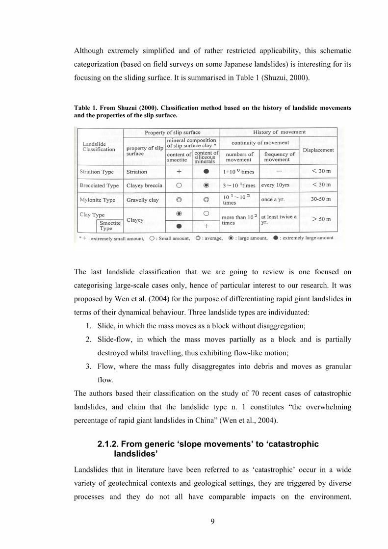
Although extremely simplified and of rather restricted applicability, this schematic

categorization (based on field surveys on some Japanese landslides) is interesting for its

focusing on the sliding surface. It is summarised in Table 1 (Shuzui, 2000).

Table 1. From Shuzui (2000). Classification method based on the history of landslide movements and the properties of the slip surface.

The last landslide classification that we are going to review is one focused on

categorising large-scale cases only, hence of particular interest to our research. It was

proposed by Wen et al. (2004) for the purpose of differentiating rapid giant landslides in

terms of their dynamical behaviour. Three landslide types are individuated:

1. Slide, in which the mass moves as a block without disaggregation;

2. Slide-flow, in which the mass moves partially as a block and is partially

destroyed whilst travelling, thus exhibiting flow-like motion;

3. Flow, where the mass fully disaggregates into debris and moves as granular

flow.

The authors based their classification on the study of 70 recent cases of catastrophic

landslides, and claim that the landslide type n. 1 constitutes “the overwhelming

percentage of rapid giant landslides in China” (Wen et al., 2004).

2.1.2. From generic ‘slope movements’ to ‘catastrophic landslides’

Landslides that in literature have been referred to as ‘catastrophic’ occur in a wide

variety of geotechnical contexts and geological settings, they are triggered by diverse

processes and they do not all have comparable impacts on the environment.

10

Nevertheless, it is possible to outline a series of features that characterise catastrophic

slope failures and may cause extensive damage, including loss of human life and

property:

• Large masses and volumes involved in sliding

• Long travel distances

• High sliding speed

• Sudden acceleration

Case studies in which one or more of the above attributes are present, but no destruction

occurs (e.g. when they take place in deserted areas) are often not referred to as

catastrophic phenomena, although they often embody the same sliding mechanisms as

destructive cases. Thus, any available field data from such cases is equally important to

the study of catastrophic landslides.

Of the reported characteristics, the primary factors on which the dangerousness of a

slope failure depends are probably the post-failure velocity and acceleration. Rapid

landslides, even those not involving large masses, have the greatest potential to cause

loss of life, because of the lack of time for the population to evacuate. A high speed

(thus corresponding to a high kinetic energy) will increase the destructive potential of

the slide, as well as the likelihood to trigger secondary and possibly more catastrophic

events. Sadly famous are the cases when slides occurred in mountainous, almost

uninhabited areas but nevertheless killed hundreds of people indirectly, by quickly

plunging into a lake and triggering devastating surge waves (Hendron and Patton, 1985,

Wieczorek et al., 2003, Yueping, 2008). If occurring underwater, the suddenness of a

landslide might trigger a violent tsunami (e.g. see Tinti et al., 2007).

Long travel distance is another dangerous characteristic, and it is very often associated

with rapid sliding. Moreover, there is a documented higher tendency for larger volumes

to reach further than expected from their energy of mass (Corominas, 1996, De Blasio et

al., 2008). On the other hand, a massive volume of soil or rock which is creeping or

sagging does not necessarily constitute a major natural hazard: certain deep-seated

alpine slides have crept for centuries before coming to a final rest, stopped for example

by topographical constraints.

It is now useful to discuss typical ranges of velocity, volume and run-out of landslides,

in an attempt to possibly establish threshold values between catastrophic and non-

catastrophic cases that may guide us in choosing the most relevant case studies.

11

Regarding the range of sliding velocities within the definition of ‘rapid’, there is no

unanimous agreement in literature. As a guidance, we can refer to the IUGS (1995)

velocity classification, reported in Table 2. While the post-failure sliding velocity, for

fast landslides, is normally measured or back-calculated as a unique average value, great

attention is given to the changes shown in slow sliding regimes, especially if

intermittent sliding (Van Genuchten, 1988) and/or accelerating displacements (Sornette

et al., 2004, Chihara et al., 1994) are observed.

Concerning the volume of the sliding mass, it is not possible to decide a critical value

enabling us to discern between catastrophic and non-catastrophic landslides, but in line

with the experience gained in reviewing several case studies (Section 2.1.4), we propose

here to consider ‘large’ any sliding mass whose volume is ≥106 m3.

At last, regarding the landslide run-out, it seems to us rather arbitrary to establish a

general threshold distinguishing between short-reach and long-reach phenomena: the

maximum ‘safe’ sliding distance will depend on the characteristics of the region (e.g.

location of inhabited areas). As a general rule, this attribute will depend on the

landslide’s volume and its vertical drop. A useful index to describe the mobility of

landslides is the angle of reach, expressed as the angle of the line connecting the head of

the landslide source to the distal margin of the displaced mass (Corominas, 1996). As

mentioned above, larger landslides usually show lower angles of reach, and because of

this they are considered more mobile. However, due to the heterogeneity of the

landslide data available in the literature it will not be possible to calculate the angle of

reach for all the case studies reviewed in Section 2.1.4.

Table 2. IUGS (1995) landslide velocity classification.

Description of velocity Velocity limits 7. Extremely rapid > 5 m/sec

6. Very rapid 3 m/min to 5 m/sec

5. Rapid 1.8 m/hour to 3 m/min

4. Moderate 13 m/month to 1.8 m/hour

3. Slow 1.6 m/year to 13 m/month

2. Very slow 16 mm/year to 1.6 m/year

1. Extremely slow ≤ 16 mm/year

12

2.1.3. Two important sub-cases: Deep-seated and flow-like movements

“In spite of their apparent diversity, deep-seated and flow-like movements may be

studied jointly. The basic impressions suggest that the two mass movement types

occupy end members of the classification spectrum , but there is a reasonable possibility

that many deep-seated landslides, now slowly moving, may represent only the initial

stage of slope movements that eventually may be transformed into accelerated sliding

and finally into large-scale, devastating rock avalanches” (Oyagi et al., 1994). Hence,

every case study in which an initial stage of coherent sliding is present, regardless of the

possible final evolution into a flow-like phenomenon, will be relevant to our landslide

data collection.

According to the literature, not exclusive diagnostic features of deep-seated slope

deformations are (Agliardi et al., 2001):

• Morpho-structures (ridges, scarps etc.) similar to those observed, at a smaller

scale, landslides occurring in cohesive soils;

• Scale of the phenomenon comparable to the size of the slope;

• Present very low rate of displacement (mm/year);

• Presence of minor landslides inside the deformed mass and ancient collapses of

the lower part of the slope.

Most of these slides do not have a macroscopically clear sliding surface, but many of

them just do not show it until final collapse. On the other hand, many observed deep-

seated slides in the Alps are in fact characterised by a basal sliding surface (Agliardi et

al., 2001), which is normally very difficult to reach.

The model that will be developed in the forthcoming chapters aims to interpret the

dynamics of sliding phenomena whilst displacing in a coherent manner, which can be

schematised by a rigid mass sliding on a basal shear localisation zone. This type of

behaviour is best represented by the early sliding stages (i.e. before breaking up into

pieces) of earth and rock slides, but our analysis will also be relevant to large landslides

whose mass, despite disintegrated, is displaced downslope for long distances whilst

preserving its stratigraphic order. For example, in sturzstroms (Section 2.1) the upper

part (often called “cap”) is “capable of travelling unmixed on top of a relatively thin

shear region, where the shear rate must become very large to account for the high

velocity of the sturzstrom” (De blasio and Elverhoi, 2008).

13

It does not appear an easy task to gather quantitative data about the coherent sliding

stage of long run-out landslides, since in most case histories geotechnical data are

available, if at all, for the final debris; i.e. after the slide has disaggregated.

Nevertheless, not only will we focus our attention on coherent sliding phenomena in our

search for data, but also on flow-like movements resulting from the transformation of an

initially coherent landslide/rockslide.

2.1.4. Landslide case studies

In this section we identify and discuss a number of terrestrial landslide case studies

found in the literature, with the aim of determining, wherever possible, relevant soil

parameter ranges that may be useful in the parametric analysis that will be developed in

Chapter 7. In the Appendix, each landslide case is summarised in a table and is assigned

a number for convenience of reference in this section. The accuracy of the cited data

relies on the quality of the drawings, plots and numbers furnished by the referenced

authors.

The examples reported in the Appendix show the extremely wide range of different

morphologies, sliding mechanisms and materials involved in fast and long run-out

landsliding, hence the difficulty in finding characteristic trends of behaviour. The

mobilisation of large rock and soil masses (>106 m3) is usually crucial to achieving

coherent long-reach sliding (in a fashion analogous to the Vajont case, n. 29, or the

Jiufengershan case, n. 1), while smaller volumes can have extended run-outs, even on

gently inclined slopes, only after transforming into flow-like slides.

Regarding sliding velocity, little data is available for the reported case studies, but the

travel classification of the majority of fast slides (i.e. belonging to categories 5, 6 or 7 of

Table 2) is ‘debris flow’ or ‘flow slide’. In fact, this is a typical evolution of large slope

movements, and it appears easier to calculate the final average sliding velocity rather

than to infer the velocity evolution during the early and intermediate sliding phases,

when the masses may still retain their original integrity. As a trend we may indicate that

for all types of landslides, all other things being equal, increasing velocities are obtained

for higher slope angles, which as common sense suggests is due to greater gravity-

dependent driving forces. On this matter Wen et al. (2004) proposed a first-

approximation power function correlating velocity and slope angle of giant landslides

occurring in China, most of which according to the authors take place on slopes dipping

between 20° and 30°.

14

On the topic of shear strength determination for the geomaterial in the slip surface, we

will focus our attention on the residual friction angle. If the material involved is clayey,

a drop in shear resistance is likely to occur after large displacements, due to the

reorientation of platy clay particles parallel to the direction of shearing. As guidance, we

refer to the experimental findings outlined by Skempton (1985) (Figure 1). If the clay

fraction (percentage in weigth of particles smaller than 0.002 mm) in the shear plane is

less than about 25%, the soil does not show significant strength drop and it behaves

much like a sand or silt, with a friction angle larger than 20°. On the contrary, when the

clay fraction is about 50%, residual strength is controlled almost entirely by sliding

friction of clay minerals. When the clay fraction is 25%-50% there is a ‘transitional’

type of behaviour, residual strength being dependent on the percentage of clay particles

as well as on their nature.

Figure 1. Residual friction angles from ring shear tests on different soils (Skempton 1985).

It is convenient to divide the treated case histories into four sub-categories, in order to

discuss them separately (the numbering adopted below refers to the landslide case

studies listed in the Appendix):

• Large masses sliding in a coherent state with long run-out

• Large masses with short run-out

• Large masses achieving a long run-out after evolving into a flow-like

phenomenon

15

• Smaller masses with high destructive potential.

2.1.4.1. Large masses sliding in a coherent state with long run-out

Erismann (1979) reports as an enigmatic feature the fact that “in many large landslides

the displaced mass, although sometimes disintegrated into small fragments, shows a

surprising congruence of its sequential order before and after the event”. This behaviour

can be mainly observed in deep-seated rotational or translational slides, especially

when the slip plane occurs in a weaker clayey layer; but also in large scale dry debris

slides (sturzstroms, cf. De Blasio et al., 2008). Such cases need to be studied with

particular concern on the frictional heat production within the slip surface, and are listed

below.

In addition to Vajont (landslide n.29), in seven more cases (landslides n. 1, 10, 24, 30,

31, 32, 33) frictional heating has been proposed as the main mechanism behind the

observed loss of shear strength, and other non-standard hypotheses have been

formulated to explain the long run-out have been formulated in 3 further cases (n. 12,

13, 26). The materials involved in these landslides are mainly sedimentary rocks (apart

from n. 10), and sliding occurs on either joint sets of unknown mineralogy (n.10, 12,

13) or on weaker clayey layers (n. 1, 9, 11, 24). The volumes involved are all large,

ranging from 106 to 109 m3. The range of residual friction angle when slip occurs on

rock joints is 27°-32°, while it can be as low as 5-10° when sliding occurs on thin clay

layers (n. 6, 9, 11, 29).

It has been widely observed in the literature (Hunter and Fell, 2003, Skempton, 1985)

that rapid sliding often occurs in strain-softening soils, such as over-consolidated clays.

Most soils with clay fraction percentage greater than 30-40% have their peak friction

angle (φp’) in the range of 22° to 30°, but they may experience a significant loss of

strength in shearing as static and dynamic friction softening occur (Tika and

Hutchinson, 1999). Skempton (1985) observed that the angles of (static) residual

shearing resistance of the three most commonly occurring clay materials are

approximately 15° for kaolinite, 10° for illite or clay mica and 5° for montmorillonite.

The special case is also contemplated where the particles smaller than 0.002 mm are

non-platy clay minerals (such as halloysite, gibbsite, bauxite, brucite, or rock flour

consisting of finely divided quartz etc.) which have high residual friction angles (>25°)

and therefore do not experience significant strain weakening (Hunter and Fell, 2003).

16

For a few case histories (n. 1, 9, 11, 29) some information about the slip surface is

given. In general in this type of slides, shear localisation occurs (e.g. see Vardoulakis,

2002a, Puzrin and Germanovich, 2005, Troncone, 2005): all deformation takes place

within a thin band of thickness of the order of some millimetres, embedded in an

otherwise thicker clay layer of homogeneous characteristics. Such clay layers where the

shearbands are localised have thicknesses of 1-10 cm, and the prevalent minerals are

chlorite, illite (n. 1, 11, 29) and montmorillonite (n. 9).

Unfortunately, little information is available on the permeability, the dynamic residual

angle and the friction-softening behaviour of the shearband materials, except for case n.

29 which appears to be the best documented one in the literature.

2.1.4.2. Large masses with short run-out

Other case histories, mostly consisting of large scale and deep seated slides, have

similar characteristics to the above type of slides; but rather than collapsing

catastrophically with sudden acceleration they exhibit a slow, creeping movement for

decades, or even centuries, before completely stopping their movement. Their final rest,

when artificial stabilisation is not carried out, can be often brought about by topographic

and morphological constraints, such as the presence of obstacles and specific shear

surface dipping conditions. On the other hand, sometimes a creeping slide is no other

than the (possibly extremely protracted in time) initial stage of a catastrophic landslide

of the type described in Section 2.1.4.1, hence deserving more consideration.

A few quantitative studies have been proposed to interpret the creeping movement of

certain deep-seated landslides such as La Clapiére (n. 2): Sornette et al. (2004) and

Helmstetter et al. (2004) proposed a “velocity law” to estimate the lifetime of the slide,

i.e. the time at which the slide will eventually collapse. Vardoulakis (2002b) and

Veveakis et al. (2007) interpreted the initial, creeping phase of Vajont (n. 1) with a

thermal-softening and velocity-strengthening law, leading to an estimation of the

collapse time of the slide. For La Frasse landslide (n. 36), Tacher et al. (2005)

developed a model able to reproduce the creeping movements during some recent

acceleration phases brought about by groundwater movement. A similar analysis was

also employed to model the mechanical behaviour of the creeping Triesenberg slide (n.

37), by Francois et al. (2007).

Due to the economical inconveniency of drilling deep core samples, less data are

available for the shear plane characteristics of deep-seated creeping slides; the attention

of researchers is usually more focused on sliding velocity and its changes over time.

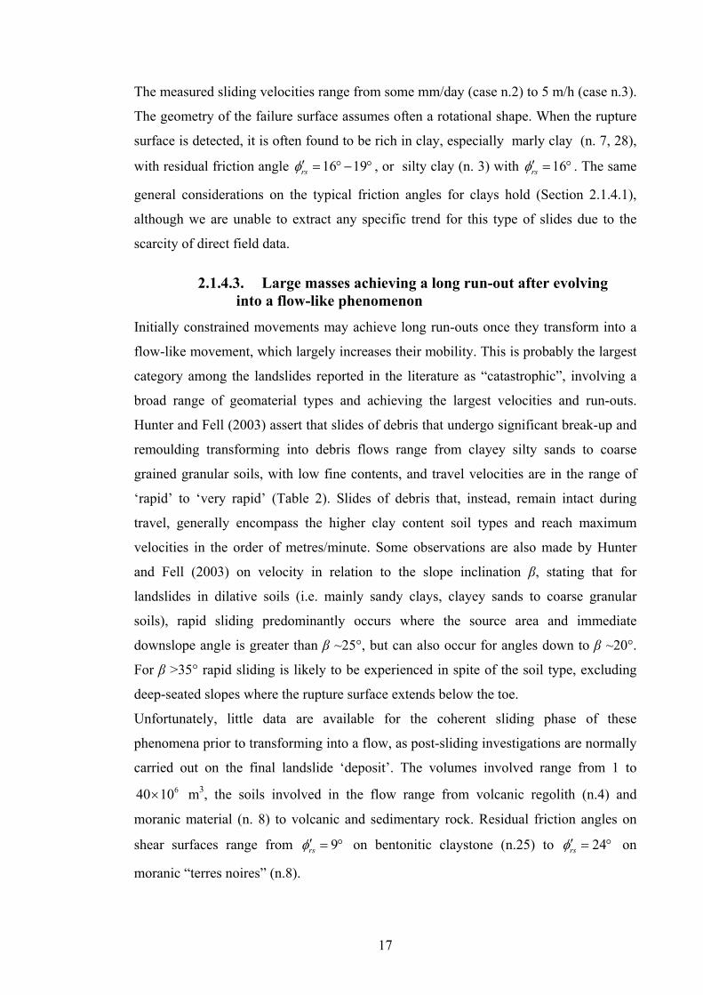
17

The measured sliding velocities range from some mm/day (case n.2) to 5 m/h (case n.3).

The geometry of the failure surface assumes often a rotational shape. When the rupture

surface is detected, it is often found to be rich in clay, especially marly clay (n. 7, 28),

with residual friction angle 16 19rsφ′ = °− ° , or silty clay (n. 3) with 16rsφ′ = ° . The same

general considerations on the typical friction angles for clays hold (Section 2.1.4.1),

although we are unable to extract any specific trend for this type of slides due to the

scarcity of direct field data.

2.1.4.3. Large masses achieving a long run-out after evolving into a flow-like phenomenon

Initially constrained movements may achieve long run-outs once they transform into a

flow-like movement, which largely increases their mobility. This is probably the largest

category among the landslides reported in the literature as “catastrophic”, involving a

broad range of geomaterial types and achieving the largest velocities and run-outs.

Hunter and Fell (2003) assert that slides of debris that undergo significant break-up and

remoulding transforming into debris flows range from clayey silty sands to coarse

grained granular soils, with low fine contents, and travel velocities are in the range of

‘rapid’ to ‘very rapid’ (Table 2). Slides of debris that, instead, remain intact during

travel, generally encompass the higher clay content soil types and reach maximum

velocities in the order of metres/minute. Some observations are also made by Hunter

and Fell (2003) on velocity in relation to the slope inclination β, stating that for

landslides in dilative soils (i.e. mainly sandy clays, clayey sands to coarse granular

soils), rapid sliding predominantly occurs where the source area and immediate

downslope angle is greater than β ~25°, but can also occur for angles down to β ~20°.

For β >35° rapid sliding is likely to be experienced in spite of the soil type, excluding

deep-seated slopes where the rupture surface extends below the toe.

Unfortunately, little data are available for the coherent sliding phase of these

phenomena prior to transforming into a flow, as post-sliding investigations are normally

carried out on the final landslide ‘deposit’. The volumes involved range from 1 to 640 10× m3, the soils involved in the flow range from volcanic regolith (n.4) and

moranic material (n. 8) to volcanic and sedimentary rock. Residual friction angles on

shear surfaces range from 9rsφ′ = ° on bentonitic claystone (n.25) to 24rsφ′ = ° on

moranic “terres noires” (n.8).

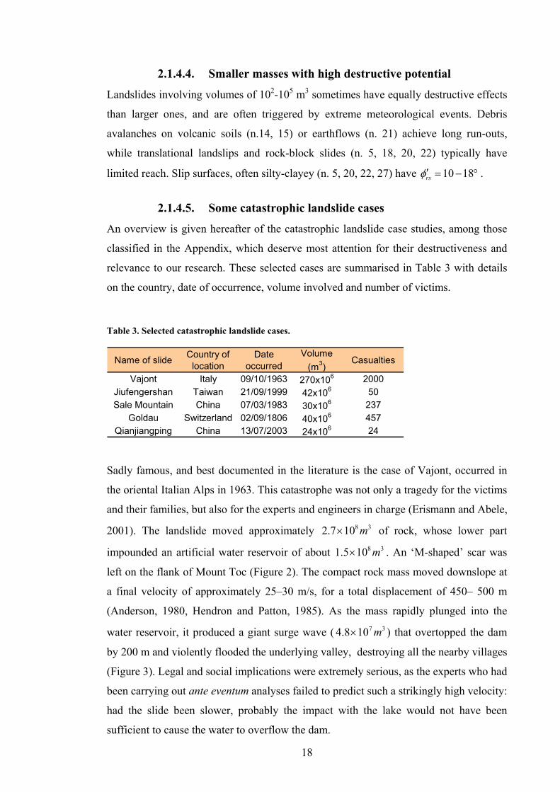
18

2.1.4.4. Smaller masses with high destructive potential

Landslides involving volumes of 102-105 m3 sometimes have equally destructive effects

than larger ones, and are often triggered by extreme meteorological events. Debris

avalanches on volcanic soils (n.14, 15) or earthflows (n. 21) achieve long run-outs,

while translational landslips and rock-block slides (n. 5, 18, 20, 22) typically have

limited reach. Slip surfaces, often silty-clayey (n. 5, 20, 22, 27) have 10 18rsφ′ = − ° .

2.1.4.5. Some catastrophic landslide cases

An overview is given hereafter of the catastrophic landslide case studies, among those

classified in the Appendix, which deserve most attention for their destructiveness and

relevance to our research. These selected cases are summarised in Table 3 with details

on the country, date of occurrence, volume involved and number of victims.

Table 3. Selected catastrophic landslide cases.

Name of slide Country of location

Date occurred

Volume (m3)

Casualties

Vajont Italy 09/10/1963 270x106 2000Jiufengershan Taiwan 21/09/1999 42x106 50Sale Mountain China 07/03/1983 30x106 237

Goldau Switzerland 02/09/1806 40x106 457Qianjiangping China 13/07/2003 24x106 24

Sadly famous, and best documented in the literature is the case of Vajont, occurred in

the oriental Italian Alps in 1963. This catastrophe was not only a tragedy for the victims

and their families, but also for the experts and engineers in charge (Erismann and Abele,

2001). The landslide moved approximately 8 32.7 10 m× of rock, whose lower part

impounded an artificial water reservoir of about 8 31.5 10 m× . An ‘M-shaped’ scar was

left on the flank of Mount Toc (Figure 2). The compact rock mass moved downslope at

a final velocity of approximately 25–30 m/s, for a total displacement of 450– 500 m

(Anderson, 1980, Hendron and Patton, 1985). As the mass rapidly plunged into the

water reservoir, it produced a giant surge wave ( 7 34.8 10 m× ) that overtopped the dam

by 200 m and violently flooded the underlying valley, destroying all the nearby villages

(Figure 3). Legal and social implications were extremely serious, as the experts who had

been carrying out ante eventum analyses failed to predict such a strikingly high velocity:

had the slide been slower, probably the impact with the lake would not have been

sufficient to cause the water to overflow the dam.

19

Scar

DamLandslide deposit

Vajont gorge

Piave valley

Figure 2. Overview of the Vajont valley after the disaster. Photo from Schrefler (2005).

Formerly Longarone village (Piave valley)

Dam

Vajont gorge

Figure 3. Historical photo of the location where the village of Longarone once stood, taken shortly after the disaster. Photo from Bojanowski (2007).

20

A similar case history to Vajont is the slide of Jiufengershan, triggered by the 1999 Chi-

Chi earthquake in Taiwan. A 6 350 10 m× mass of sandstone and shale detached from a

mountain flank (Figure 4) and travelled downslope at high velocity in a translational

fashion for a total displacement of about 1 km. The debris deposit dammed two creeks

and created three small lakes upstream (Chang et al., 2005). Several post eventum

investigations were carried out on this slide, so that an adequate amount of data on the

soil properties and in-situ conditions of the slope is available in the literature.

The Sale Mountain compound landslide, occurred in China in 1985, is yet another

example of a giant rockslide that moved in a coherent fashion at an unexpectedly high

velocity: in less than one minute the mass travelled 1 km (Zhang et al., 2002). Similarly

to Vajont, deformation was found to be localised in a 2 mm thick shear band while the

overburden moved as a rigid block, to the extent that an eyewitness of the event saved

his life by hanging on to a tree and travelling with it for about 960m on the surface of

the sliding mass. Even though a quantitative back-analysis of this event has been

published (Miao et al., 2001), there is a certain lack of essential geotechnical data in the

literature.

Figure 4. From Shou and Wang (2003). The planar slide of Jiufengershan, occurred in Taiwan in 1999.

Despite having happened two centuries ago, the Goldau landslide is one of the best

known ones of the Swiss Alps (Figure 5). Historical documents report the suddenness

21

and large size of the event, although the availability of quantitative data is very limited.

Nevertheless, the sliding mode and conjectures of frictional heating in the slip plane

(Erismann, 1979) make Goldau an interesting case to our research.

Figure 5. From Thuro et al. (2005). the Goldau landslide in a painting by H. Keller, 1806.

Figure 6. From Yueping (2008). Overview of Qiangjiangping slide, occurred in 2003 in China.

22

(a)

(b)

Figure 7. From Yueping (2008). Qiangjiangping landslide: (a) Sections of the slope before and after the slide and (b) photo of the slip surface.

It is finally worth mentioning the recent Qiangjiangping case (Figure 6), which

analogously to Vajont was a reactivated slide, triggered by reservoir filling during the

completion of the renowned Three Gorges hydro-electric project. A fast slip rate (1 m/s

on average according to Wen et al., 2004) was reported for this event, which (unlike

23

Vajont) was not enough to generate significant waves by impacting the water.

Unfortunately though, the debris rapidly dammed the underlying river, and a 30 m high

surge was created subsequently upon dam breaching, killing 24 people in the

surrounding shores. The geometry of this slide is clear (Figure 7), but no geotechnical

data are available at the time of writing.

2.2. Submarine landslide cases

2.2.1. Classification of submarine landslides

Submarine landslides in the world are as frequent as their terrestrial counterparts. They

are often cause of major disasters, involving loss of property and life, notably when they

act as triggers of tsunamis or they impact on inhabited coastal areas. Many other

submarine landslides go unnoticed, but the potential impact of these phenomena is

increasing as Man is expanding in the oceans, building new oil and gas platforms and

searching areas to dispose of nuclear waste. Moreover, undersea slope failures are of

great interest to the scientific research community in understanding some still obscure

mechanisms of movement, leading to substantial modification of continental margins.

Most of the terminology applied to submarine slides normally comes from that applied

to terrestrial slides, but it is necessary to make distinctions to avoid confusion, as

submarine phenomena are different in some aspects. Besides, it is difficult to provide an

ad hoc classification as sub-oceanic movements have hardly ever been directly

observed, thus it is extremely uncertain to infer deformational mechanisms and

processes from the landslide geometry observed after the particular event. In fact, it may

happen that many different deformational characteristics involved in the movement

which are not preserved in the final configuration of the landslide.

Many authors, among which Canals et al. (2004), Lee et al. (1991) and Prior (1988)

point out the aforementioned confusion in terms commonly used in underwater geology,

for example in the overuse of the term ‘slump’, which should correctly only indicate the

specific kind of sliding with rotational movement.

A brief and simple classification (Prior 1988), following concepts developed from

terrestrial landslides is schematised in Figure 8, and comprises a continuum of slides

and flows. The movement types can be described as follows.

• Slides consist of a mass sliding over one or more discrete basal shear planes,

often occurring on slopes of less than 5 degrees. They often involve very large

volumes, and can be subdivided according to the geometry of shear surfaces into

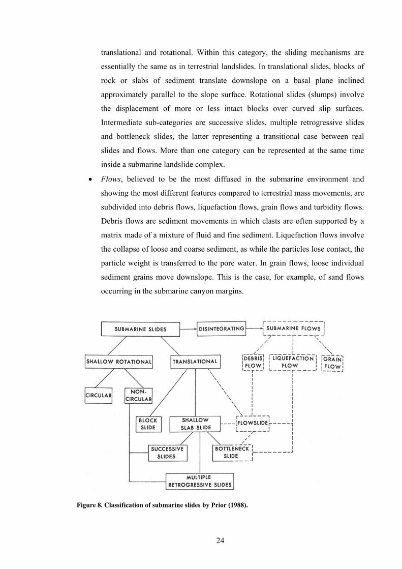
24

translational and rotational. Within this category, the sliding mechanisms are

essentially the same as in terrestrial landslides. In translational slides, blocks of

rock or slabs of sediment translate downslope on a basal plane inclined

approximately parallel to the slope surface. Rotational slides (slumps) involve

the displacement of more or less intact blocks over curved slip surfaces.

Intermediate sub-categories are successive slides, multiple retrogressive slides

and bottleneck slides, the latter representing a transitional case between real

slides and flows. More than one category can be represented at the same time

inside a submarine landslide complex.

• Flows, believed to be the most diffused in the submarine environment and

showing the most different features compared to terrestrial mass movements, are

subdivided into debris flows, liquefaction flows, grain flows and turbidity flows.

Debris flows are sediment movements in which clasts are often supported by a

matrix made of a mixture of fluid and fine sediment. Liquefaction flows involve

the collapse of loose and coarse sediment, as while the particles lose contact, the

particle weight is transferred to the pore water. In grain flows, loose individual

sediment grains move downslope. This is the case, for example, of sand flows

occurring in the submarine canyon margins.

Figure 8. Classification of submarine slides by Prior (1988).

25

Another classification of subaqueous landslides was proposed by Lee et al. (1991),

based on the modification of that by Varnes (1978), effectively synthesised in Figure 9.

While the ‘slides’ part, which in turn mirrors the terrestrial slides case, is analogous to

the previous classification, the ‘mass flows’ part contains more detailed observations.

Slides can often transform into flows as the sliding mass progressively disintegrates

while moving downslope. Mudflows are similar to debris flows, but they involve

muddy sediments. Turbidity currents, represented in the last drawing on the right in

Figure 9, involve the transport of a relatively diluted suspension of sediment grains

supported by an upward component of fluid turbulence.

Figure 9. Classification of submarine slides by Lee et al. (1988).

Figure 10. Events that are likely to trigger submarine slides by reducing their safety factor (Locat and Lee, 2000).

2.2.2. Typical environments and causes of submarine landslides

A schematic list of possible factors which are prone to initiate submarine landslides

based on conventional stability analysis can be seen in Figure 10 (Locat and Lee, 2000).

26

It can be noted, first of all, that some of the causes, such as gas charging and wave

loading, are peculiar to the subaqueous environment. In general, a landslide occurs

when the downslope driving stress exceeds the resisting strength of the material. The

action of gravity is obviously common to all environments, as the seafloor is always

relatively inclined, but gravity is not the unique factor.

Hampton et al. (1996) proposed a comprehensive account of the typical “submarine

landslide territory”, consisting of five environments, listed below.

• Fjords. These submerged glacially eroded valleys usually have a sediment-laden

river delta at the head. The sediment deposition rate on the delta can outpace the

expulsion of pore water, which determines a low static shear strength due to

under-consolidation. The typically rocky sediment is also predisposed to loss of

strength under the load of waves and possible earthquakes.

• River deltas on the continental margin. Subaqueous slope failures are common

in those areas of the continental margin where a river mouth provides a point

source entry of sediment. Specific conditions are needed for slope failure to

occur in deltas. High sedimentation rate is necessary in order to accumulate a

sufficiently thick bed of sediment. The sediment is often fine-grained or plastic,

so that the low permeability can allow to retain pore pressure and as a result to

produce under-consolidation as in the above case. Key factors to trigger these

processes are environmental loads, such as wave storms and earthquakes.

• Submarine Canyons. Canyons are very frequent underwater and their tall and

steep side walls facilitate the insurgence of landslides, which in turn are

responsible for the continuous shape evolution of canyons. Mass movements are

caused by gravity and internally derived seepage forces.

• Open continental margin. Typical slopes of 3-6 degrees determine a tendency

for gravity-driven mass movements in these areas, off the continents and larger

islands. Apart from some areas of high tectonic steepening, gravity is not

normally reputed to be great enough to cause failure. Causes can be earthquake

shaking, effects of rapidly changing sea level and gas hydrate dissociation.

• Oceanic volcanic islands and ridges. Some of the biggest existing landslides

occur on the flanks of volcanic islands, caused by still poorly understood factors.

Earthquakes in this case are more a consequence than a cause of volcanic

27

landslides, and the mechanisms may be related to the inherently unstable

structure of volcanic islands.

Other causes listed by Hampton et al. (1996) which have been proposed for the

occurrence of submarine landslides are tectonic processes, such as faults and

subduction, oversteepening of tall carbonate slopes and biologic weakening processes.

2.2.3. Similarities and differences between terrestrial and submarine landslides

The morphology and mechanics of the two kind of landslides have many similarities,

but also important differences.

Firstly, subaqueous landslides can be much larger than their sub-aerial counterparts, the

largest of which displace masses of the order of 20-25 cubic kilometres. By comparison,

the largest submarine mass movements have involved volumes up to 20,000 km3 as a

single failure event (Hampton et al., 1996). As an example, the well-documented

Storegga slide off the coast of Norway (Bugge et al. 1988) has a volume of 5000 km3.

Secondly, the sliding run-out is also normally much larger for underwater events, often

being of the order of hundredths of km.

Thirdly, gravity has a less significant role as a driving force, under water. Submarine

landslides can originate on virtually flat surfaces. Examples of low slope angle failures

include the Mississipi river delta slide and Klamath river delta slide, characterised by

slope angles of 0.1-0.4° and 0.25° respectively (Leroueil, 1996 and Locat et al., 1996).

Legros (2002) compared terrestrial and submarine slides in graphs representing the ratio

of the total drop height Hmax and the runout distance Lmax plotted against the mass

volume V (Figure 11a). The difference is striking as subaqueous slides show a much

lower ratio Hmax/Lmax. This is explained by Legros (2002) with the larger mobility of

submarine landslides as a consequence of their mixing with large amounts of water.

Plotting Lmax against V (Figure 11b) shows, however, that the two types of landslides

follow exactly the same trend. A possible interpretation of this is that Lmax is essentially

a function of V, with Hmax only being of minor influence; which suggests the similarity

in the emplacement mechanisms of the two types of landslides, despite the different

environments. There is a documented higher tendency for underwater phenomena to

transform into flows, hence the longer run-outs. Some submarine debris flows convert

into turbidity currents by incorporating overlying sea water, so that the remoulded shear

strength of the material in the starting zone can be much higher than the strength of the

flowing debris flow (Leroueil et al 1996). In such cases, the surrounding water plays an

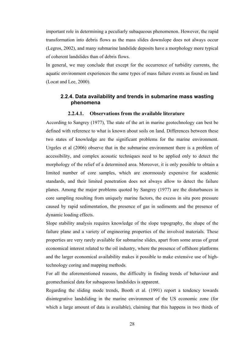
28

important role in determining a peculiarly subaqueous phenomenon. However, the rapid

transformation into debris flows as the mass slides downslope does not always occur

(Legros, 2002), and many submarine landslide deposits have a morphology more typical

of coherent landslides than of debris flows.

In general, we may conclude that except for the occurrence of turbidity currents, the

aquatic environment experiences the same types of mass failure events as found on land

(Locat and Lee, 2000).

2.2.4. Data availability and trends in submarine mass wasting phenomena

2.2.4.1. Observations from the available literature

According to Sangrey (1977), The state of the art in marine geotechnology can best be

defined with reference to what is known about soils on land. Differences between these

two states of knowledge are the significant problems for the marine environment.

Urgeles et al (2006) observe that in the submarine environment there is a problem of

accessibility, and complex acoustic techniques need to be applied only to detect the

morphology of the relief of a determined area. Moreover, it is only possible to obtain a

limited number of core samples, which are enormously expensive for academic

standards, and their limited penetration does not always allow to detect the failure

planes. Among the major problems quoted by Sangrey (1977) are the disturbances in

core sampling resulting from uniquely marine factors, the excess in situ pore pressure

caused by rapid sedimentation, the presence of gas in sediments and the presence of

dynamic loading effects.

Slope stability analysis requires knowledge of the slope topography, the shape of the

failure plane and a variety of engineering properties of the involved materials. These

properties are very rarely available for submarine slides, apart from some areas of great

economical interest related to the oil industry, where the presence of offshore platforms

and the larger economical availability makes it possible to make extensive use of high-

technology coring and mapping methods.

For all the aforementioned reasons, the difficulty in finding trends of behaviour and

geomechanical data for subaqueous landslides is apparent.

Regarding the sliding mode trends, Booth et al. (1991) report a tendency towards

disintegrative landsliding in the marine environment of the US economic zone (for

which a large amount of data is available), claiming that this happens in two thirds of

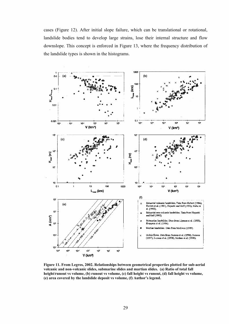
29

cases (Figure 12). After initial slope failure, which can be translational or rotational,

landslide bodies tend to develop large strains, lose their internal structure and flow

downslope. This concept is enforced in Figure 13, where the frequency distribution of

the landslide types is shown in the histograms.

(a) (b)

(c) (d)

(e)

(f)

Figure 11. From Legros, 2002. Relationships between geometrical properties plotted for sub-aerial volcanic and non-volcanic slides, submarine slides and martian slides. (a) Ratio of total fall height/runout vs volume, (b) runout vs volume, (c) fall height vs runout, (d) fall height vs volume, (e) area covered by the landslide deposit vs volume, (f) Author’s legend.

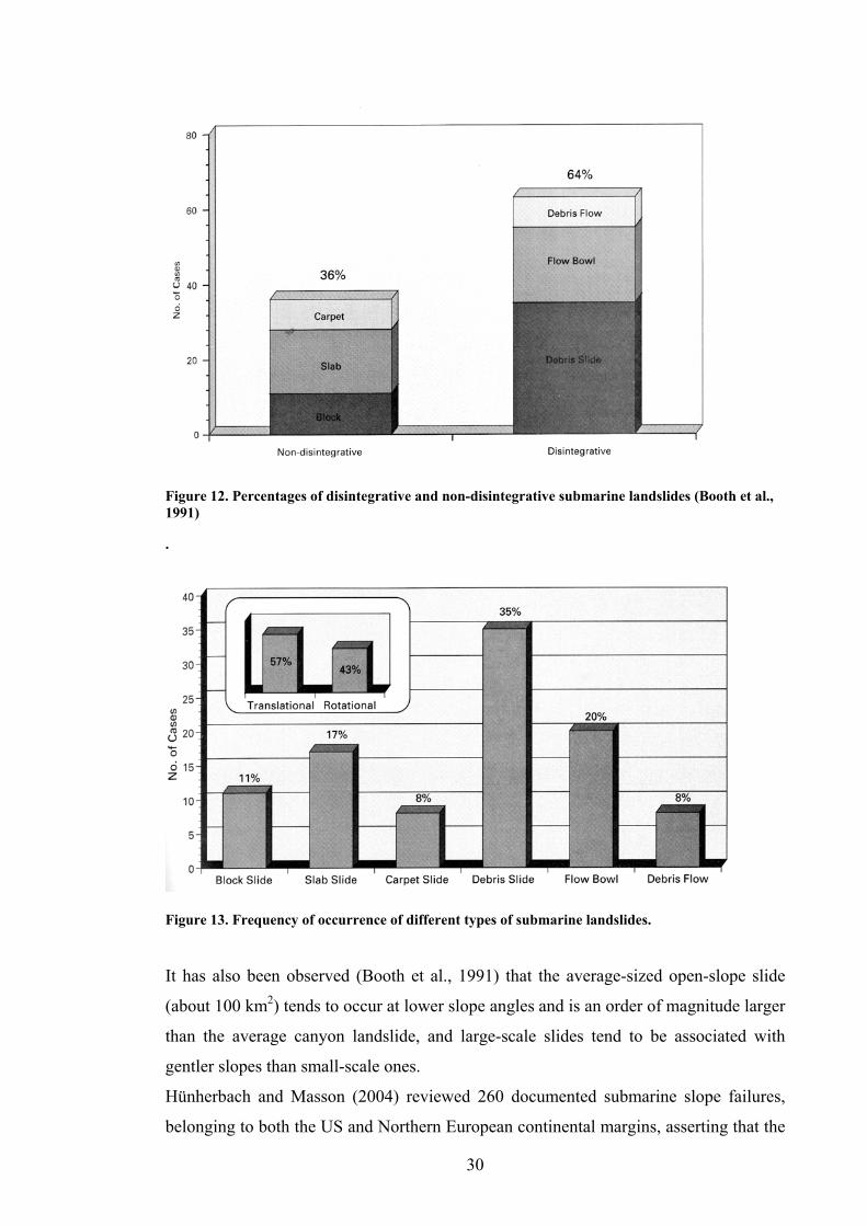
30

Figure 12. Percentages of disintegrative and non-disintegrative submarine landslides (Booth et al., 1991)

.

Figure 13. Frequency of occurrence of different types of submarine landslides.

It has also been observed (Booth et al., 1991) that the average-sized open-slope slide

(about 100 km2) tends to occur at lower slope angles and is an order of magnitude larger

than the average canyon landslide, and large-scale slides tend to be associated with

gentler slopes than small-scale ones.

Hünherbach and Masson (2004) reviewed 260 documented submarine slope failures,

belonging to both the US and Northern European continental margins, asserting that the

31

only parameters that are sufficiently available to be discussed in detail are (a)

dimensions, (b) slope angle, (c) total height, (d) headwall height and (e) water depth.

After a statistical analysis of not always complete database entries, the authors could

conclude the following:

• The slope angle does not influence the occurrence of subaqueous landslides, also

given that the largest ones appear to occur on the lowest slopes.

• On both sides of the Atlantic continental margin, there appears to be a peak in

landslide headwall location at a depth of about 1000-1300 m, suggesting the

presence of specific weak layers prone to failure.

• Landslides in fjords tend to be disintegrative.

• Geotechnical measurements and sediment rheology are seldom available.

It is finally worth reporting here the observation of Silva et al. (2004) that one of the

most important differences between marine and terrestrial sediments is the generally

less significant spatial variation of engineering properties in marine sediments, implying

that soil properties of subaqueous deposits are often similar over large areas. This

means that the need for systematic sampling can be smaller.

2.2.4.2. Data collection

We have collected as many case studies of submarine slides as possible in which

geomechanical properties were measured or deducted, in an attempt to collate data and

associate soil properties and mineralogy with landslide behaviour.

Some of the best documented case studies, among those occurring in deep-water, are the

Storegga slide off the coast of Norway (Bugge et al., 1988, Kvalstad et al., 2005a,

2005b, Forsberg and Locat 2005), the Gebra, Finneidfjord and Afen slides (Canals et

al., 2004), the Gulf of Mexico slides (Silva et al., 2004), the Canary slide (Roberts and

Cramp, 1996, Canals et al., 2004), the Ebro Slope slide (Urgeles et al. 2006), the North

Aegean trough slide (Lykousis et al. 2002) and the Hudson Apron flowslide (Desgagnes

et al. 2000). Better documented, for obvious practical reasons, are the few case studies

of landslides which initiated on the coast and terminated under water, or those involving

parts of coast due to retrogressive behaviour of the submarine landslide (Cornforth and

Lowell 1996). Some examples of the kind of available data follow below.

Mineralogy is known for the Hudson Apron slide (silty clay, clay fraction 37-60%,

composed of illite, chlorite and little smectite), the undrained shear strength is measured

(0.5 to 15 kPa) and a probable failure plane was detected at a depth of 20 metres;

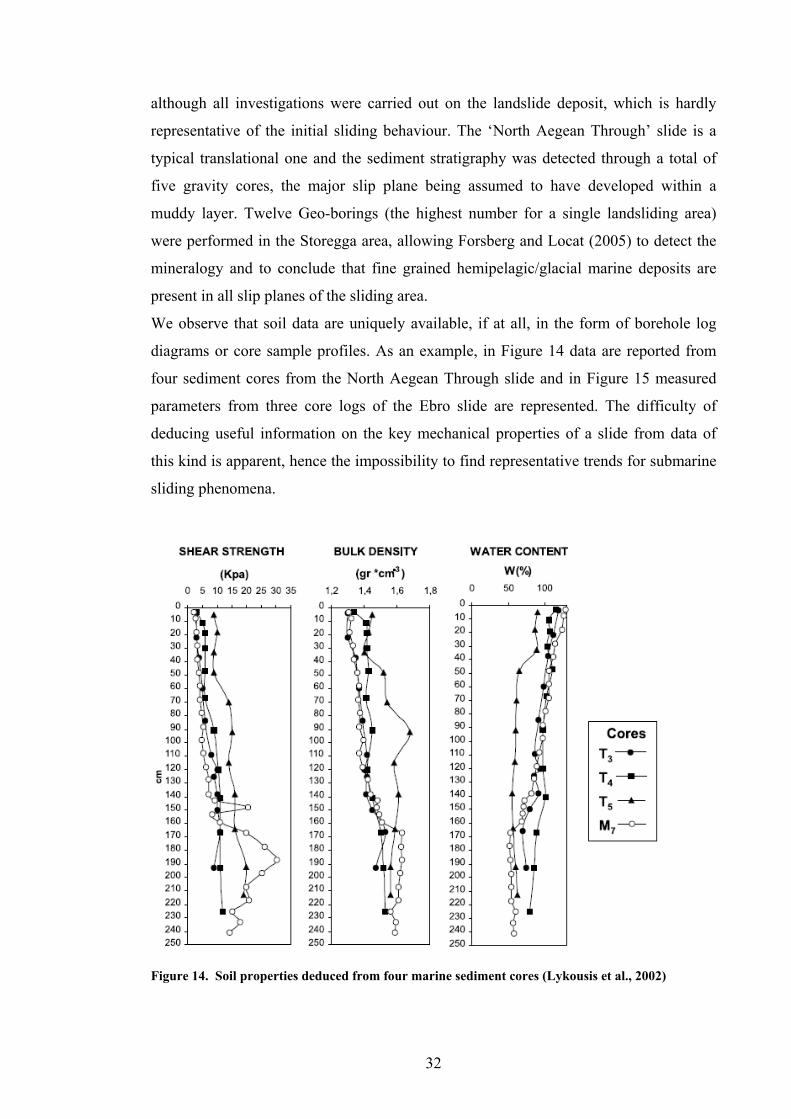
32

although all investigations were carried out on the landslide deposit, which is hardly

representative of the initial sliding behaviour. The ‘North Aegean Through’ slide is a

typical translational one and the sediment stratigraphy was detected through a total of

five gravity cores, the major slip plane being assumed to have developed within a

muddy layer. Twelve Geo-borings (the highest number for a single landsliding area)

were performed in the Storegga area, allowing Forsberg and Locat (2005) to detect the

mineralogy and to conclude that fine grained hemipelagic/glacial marine deposits are

present in all slip planes of the sliding area.

We observe that soil data are uniquely available, if at all, in the form of borehole log

diagrams or core sample profiles. As an example, in Figure 14 data are reported from

four sediment cores from the North Aegean Through slide and in Figure 15 measured

parameters from three core logs of the Ebro slide are represented. The difficulty of

deducing useful information on the key mechanical properties of a slide from data of

this kind is apparent, hence the impossibility to find representative trends for submarine

sliding phenomena.

Figure 14. Soil properties deduced from four marine sediment cores (Lykousis et al., 2002)

33

Figure 15. Example of submarine core logs data (Urgeles et al, 2006).

2.2.4.3. Relevance of submarine landslides to our research

For submarine landslides, unlike their sub-aerial counterparts, it has not been possible to

find reasonable ranges of soil parameters which could be considered representative of

particular submarine sliding modes and used for the calibration of the new landslide

model (cf. Chapters 5, 6 and 7), as the available properties are scattered, uncertain and

too small in number.

We have seen, however, some subaqueous mass displacement phenomena exhibiting

coherent sliding, like submarine ‘block slides’ and ‘slab slides’ (Lee et al., 1991). Even

flow-like phenomena and turbidity currents can have a relatively short phase,

immediately after failure, of coherent sliding.

Regarding the most relevant phenomena to us, we would exclude river delta slides, and

probably fjord landslides as well, as these are normally brought about by sediment

underconsolidation which constitutes a unique marine mechanism. All other marine

mass wasting phenomena on the contrary, especially slides occurring in the open

continental margin, are to be considered of maximum significance to our research, as a

dynamic landslide model accounting for frictional heating could in principle be

employed interpret the initial (coherent) phase of their sliding.

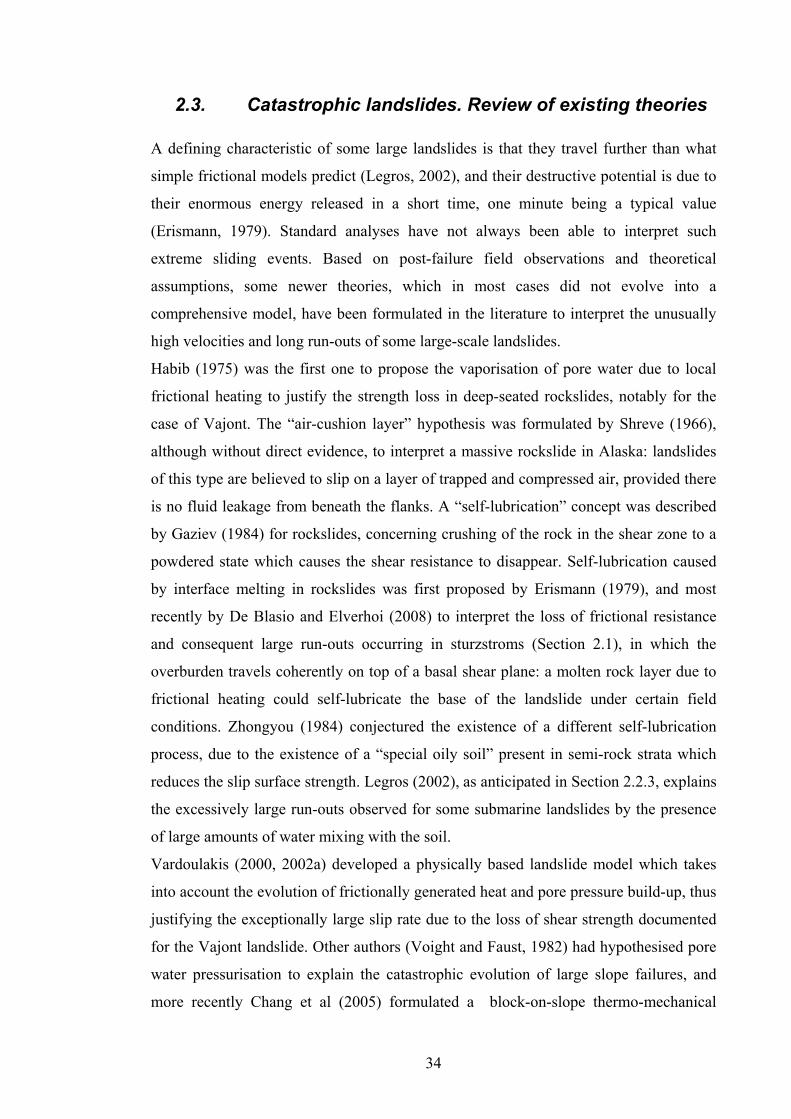
34

2.3. Catastrophic landslides. Review of existing theories

A defining characteristic of some large landslides is that they travel further than what

simple frictional models predict (Legros, 2002), and their destructive potential is due to

their enormous energy released in a short time, one minute being a typical value

(Erismann, 1979). Standard analyses have not always been able to interpret such

extreme sliding events. Based on post-failure field observations and theoretical

assumptions, some newer theories, which in most cases did not evolve into a

comprehensive model, have been formulated in the literature to interpret the unusually

high velocities and long run-outs of some large-scale landslides.

Habib (1975) was the first one to propose the vaporisation of pore water due to local

frictional heating to justify the strength loss in deep-seated rockslides, notably for the

case of Vajont. The “air-cushion layer” hypothesis was formulated by Shreve (1966),

although without direct evidence, to interpret a massive rockslide in Alaska: landslides

of this type are believed to slip on a layer of trapped and compressed air, provided there

is no fluid leakage from beneath the flanks. A “self-lubrication” concept was described

by Gaziev (1984) for rockslides, concerning crushing of the rock in the shear zone to a

powdered state which causes the shear resistance to disappear. Self-lubrication caused

by interface melting in rockslides was first proposed by Erismann (1979), and most

recently by De Blasio and Elverhoi (2008) to interpret the loss of frictional resistance

and consequent large run-outs occurring in sturzstroms (Section 2.1), in which the

overburden travels coherently on top of a basal shear plane: a molten rock layer due to

frictional heating could self-lubricate the base of the landslide under certain field

conditions. Zhongyou (1984) conjectured the existence of a different self-lubrication

process, due to the existence of a “special oily soil” present in semi-rock strata which

reduces the slip surface strength. Legros (2002), as anticipated in Section 2.2.3, explains

the excessively large run-outs observed for some submarine landslides by the presence

of large amounts of water mixing with the soil.

Vardoulakis (2000, 2002a) developed a physically based landslide model which takes

into account the evolution of frictionally generated heat and pore pressure build-up, thus

justifying the exceptionally large slip rate due to the loss of shear strength documented

for the Vajont landslide. Other authors (Voight and Faust, 1982) had hypothesised pore

water pressurisation to explain the catastrophic evolution of large slope failures, and

more recently Chang et al (2005) formulated a block-on-slope thermo-mechanical

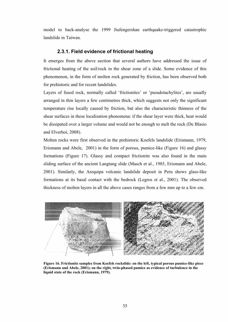
35

model to back-analyse the 1999 Jiufengershan earthquake-triggered catastrophic

landslide in Taiwan.

2.3.1. Field evidence of frictional heating

It emerges from the above section that several authors have addressed the issue of

frictional heating of the soil/rock in the shear zone of a slide. Some evidence of this

phenomenon, in the form of molten rock generated by friction, has been observed both

for prehistoric and for recent landslides.

Layers of fused rock, normally called ‘frictionites’ or ‘pseudotachylites’, are usually

arranged in thin layers a few centimetres thick, which suggests not only the significant

temperature rise locally caused by friction, but also the characteristic thinness of the

shear surfaces in these localisation phenomena: if the shear layer were thick, heat would

be dissipated over a larger volume and would not be enough to melt the rock (De Blasio

and Elverhoi, 2008).

Molten rocks were first observed in the prehistoric Koefels landslide (Erismann, 1979,

Erismann and Abele, 2001) in the form of porous, pumice-like (Figure 16) and glassy

formations (Figure 17). Glassy and compact frictionite was also found in the main

sliding surface of the ancient Langtang slide (Masch et al., 1985, Erismann and Abele,

2001). Similarly, the Arequipa volcanic landslide deposit in Peru shows glass-like

formations at its basal contact with the bedrock (Legros et al., 2001). The observed

thickness of molten layers in all the above cases ranges from a few mm up to a few cm.

Figure 16. Frictionite samples from Koefels rockslide: on the left, typical porous pumice-like piece (Erismann and Abele, 2001); on the right, twin-phased pumice as evidence of turbulence in the liquid state of the rock (Erismann, 1979).

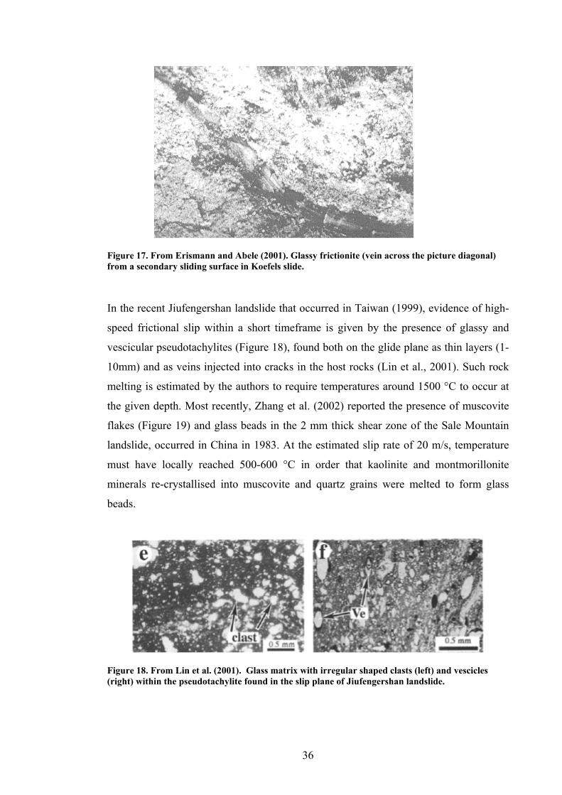
36

Figure 17. From Erismann and Abele (2001). Glassy frictionite (vein across the picture diagonal) from a secondary sliding surface in Koefels slide.

In the recent Jiufengershan landslide that occurred in Taiwan (1999), evidence of high-

speed frictional slip within a short timeframe is given by the presence of glassy and

vescicular pseudotachylites (Figure 18), found both on the glide plane as thin layers (1-

10mm) and as veins injected into cracks in the host rocks (Lin et al., 2001). Such rock

melting is estimated by the authors to require temperatures around 1500 °C to occur at

the given depth. Most recently, Zhang et al. (2002) reported the presence of muscovite

flakes (Figure 19) and glass beads in the 2 mm thick shear zone of the Sale Mountain

landslide, occurred in China in 1983. At the estimated slip rate of 20 m/s, temperature

must have locally reached 500-600 °C in order that kaolinite and montmorillonite

minerals re-crystallised into muscovite and quartz grains were melted to form glass

beads.

Figure 18. From Lin et al. (2001). Glass matrix with irregular shaped clasts (left) and vescicles (right) within the pseudotachylite found in the slip plane of Jiufengershan landslide.

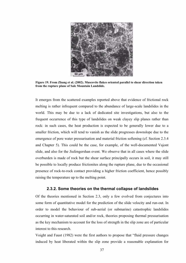
37

Figure 19. From Zhang et al. (2002). Muscovite flakes oriented parallel to shear direction taken from the rupture plane of Sale Mountain Landslide.

It emerges from the scattered examples reported above that evidence of frictional rock

melting is rather infrequent compared to the abundance of large-scale landslides in the

world. This may be due to a lack of dedicated site investigations, but also to the

frequent occurrence of this type of landslides on weak clayey slip planes rather than

rock: in such cases, the heat production is expected to be generally lower due to a

smaller friction, which will tend to vanish as the slide progresses downslope due to the

emergence of pore water pressurisation and material friction softening (cf. Section 2.3.4

and Chapter 5). This could be the case, for example, of the well-documented Vajont

slide, and also for the Jiufengershan event. We observe that in all cases where the slide

overburden is made of rock but the shear surface principally occurs in soil, it may still

be possible to locally produce frictionites along the rupture plane, due to the occasional

presence of rock-to-rock contact providing a higher friction coefficient, hence possibly

raising the temperature up to the melting point.

2.3.2. Some theories on the thermal collapse of landslides

Of the theories mentioned in Section 2.3, only a few evolved from conjectures into

some form of quantitative model for the prediction of the slide velocity and run-out. In

order to model the behaviour of sub-aerial (or submarine) catastrophic landslides

occurring in water-saturated soil and/or rock, theories proposing thermal pressurisation

as the key mechanism to account for the loss of strength in the slip zone are of particular

interest to this research.

Voight and Faust (1982) were the first authors to propose that “fluid pressure changes

induced by heat liberated within the slip zone provide a reasonable explanation for

38

dynamic problems implied by some high-speed landslides”. While Habib (1967) had

theorised vaporisation of pore water and subsequent creation of a gas cushion to justify

the loss of shear strength in the slip plane, Voight and Faust (1982) proposed that

substantial strength loss would happen due to a mere rise in pore water pressure,

without the need for water to change phase. The authors presented a first-attempt model

for evaluating the pore pressure changes and temperature rise during a rapid land sliding

event. Under the substantially simplifying assumptions that due to high slip rate, heat

and excess pore pressure do not have the time to diffuse away of the slip zone, the

mathematical model was solved analytically and a parametric study was presented to

qualitatively highlight the basic implications of frictional heating and pore pressure

build-up:

• As the effective stress across the fault vanishes, so also does the increase in

frictional heat, due to the concurrent reduction of friction.

• The temperature rise during sliding is greater for larger initial effective normal

stresses.

• The temperature and pore pressure rise depend on the ratio between slide

displacement and shear zone thickness.

Calculations were also made alongside the parametric study in an attempt to match the

final velocity of the Vajont case, showing that despite the strong simplifications, a

model involving pressurisation and frictional heating can provide a rational explanation

for the observed extremely low values of apparent kinetic friction. Nevertheless, in the

description of the strength loss mechanism no account was taken for displacement and

velocity softening (i.e. the decrease in the soil friction coefficient with increasing

displacement and velocity), while this phenomenon is widely acknowledged and was

subsequently shown to occur in the clayey soil of Vajont (Tika and Hutchinson, 1999).

More recently, Chang et al. (2005) presented a quantitative analysis of earthquake-

triggered landsliding by resorting to thermo-mechanics. Thermal pressurisation, whose

occurrence is possible in low permeability shear zones (e.g. clayey materials),

determines the evolution of the shear strength during the sliding process. Starting from

some field evidence of high pore pressures developed within the sliding body (near the

main shear zone, mud injections infilling pre-existing fractures and joints had been

observed in the landslide material), the authors formulated a block-on-slope model to

study both the triggering and the propagation phase of the Jiufengershan catastrophic

landslide. The model accounts for the partial transformation of frictional energy into

39

heat through a parameter called “thermal absorption coefficient”, and subsequent

temperature rise within the shearing zone. A parametric analysis is then presented, in

which the kinematical parameters of a sliding block are calculated and different

scenarios are examined depending on selected values of pore pressure and thermal

absorption coefficient. In the “avalanche regime” case, representing the catastrophic

sliding scenario which matches the field observations for the Jiufengershan slide, the

block acquires a maximum velocity of 80 m/s and the final fault plane temperature

reaches 113 °C. The time evolution of pore pressures and shear stress within the slip

plane is also calculated. These results confirm the importance of the thermal

pressurisation mechanism in interpreting high-speed sliding, as emerged in the

preceding literature. Nevertheless, the proposed model equations are not able to

interpret in a self-consistent manner the landslide motion coupled with the equations for

heat flow and pore pressure evolution across the shear zone, and do not therefore appear

as suitable a basis for constitutive improvements and future generalisation as the

governing equations of Vardoulakis (2002a), which will be presented with more detail

in Section 2.3.4.

2.3.3. The mechanism of thermal pressurisation

Frictional heating and thermal pressurisation are believed to be responsible for the

weakening of shear resistance in a variety of contexts, when the material under

consideration is subjected to relatively rapid temperature changes: from the reservoir

rock involved in petroleum drilling and deep geological formations destined to store

radioactive waste to rapid fault slip events, either due to tectonic (seismic) forces within

the Earth crust or driven by gravity (landsliding) on the Earth surface. While the reason

for heat production due to friction in the slip plane is rather intuitive, the mechanism of

pressurisation deserves more attention since it manifests itself in different forms

depending on the geomaterial in question.

Thermal pressurisation has been largely studied, especially when it occurs in rock

leading to shear failure or hydraulic fracturing. Thermal weakening of rock faults during

co-seismic slip has been extensively reviewed by Rice (2006), while Wibberley and

Shimamoto (2005) and Sulem et al. (2007) have dealt with the thermal collapse of clay

materials in fault zones. Vardoulakis (2000, 2002a), as mentioned in Section 2.3, has

studied thermal pressurisation in clayey gouges with application to the dynamic

behaviour of rapid landslides. Some experimental evidence of thermal pressurisation in

40

both rocks and soils has been collected, among others, by Campanella and Mitchell

(1968), Baldi et al. (1988), Sultan (1997), Sultan et al. (2002), Ghabezloo and Sulem

(2008).

Efforts have been made in the literature to measure or calculate an average value for the

key parameter that governs thermal pressurisation, which is the pressurisation

coefficient λm, defined as the pore pressure increase due to a unit temperature increase

under undrained conditions (at constant specific volume). It has emerged that this

coefficient is far from being constant but depends on the considered material, in

addition to the temperature and the stress level. Different average values for λm have

been proposed, ranging two of orders of magnitude. For clay, Campanella and Mitchell

(1968) found λm=0.01 MPa/°C, Vardoulakis (2002a) proposed λm=0.06 MPa/°C while

Sulem et al. (2007) suggested λm=0.1 MPa/°C. For sandstone, Campanella and Mitchell

(1968) proposed λm=0.05 MPa/°C while Rice (2006) estimated λm=0.92 MPa/°C for a 7

km deep fault in rock with intact walls.

A substantial difference in the thermal pressurisation mechanisms emerges between clay

and rock materials: while rocks essentially behave elastically and λm is found to depend

on thermo-elastic coefficients only, clays may undergo plastic straining upon thermal

loading, giving rise to an additional dependency for λm on the soil’s thermo-plastic

contraction coefficient.

For rocks, the coefficient λm can be expressed as

( ) ( )m f n f nc cλ α α= − + (1.1)

(Rice, 2006), where the α’s are thermo-elastic expansion coefficients, the c’s

compressibility coefficients and the subscripts f and n denote the pore fluid and the pore

volume respectively. By looking at the numerator of Equation (1.1), the physics behind

thermo-elastic pressurisation are evident: pore pressure increases due to the fluid

exhibiting a higher thermal volume increase than the pore space, i.e. the pressurisation

mechanism depends on the differential expansion of the fluid and the pore space.

Experimental results for granular rock (Ghabezloo and Sulem, 2008) draw attention to

the dependency of the pressurisation coefficient on stress and temperature. The latter

has an influence on λm mainly due to the thermal increase of expansion coefficients, the

former is important due to the stress-dependent character of the pore volume

compressibility cn. As a consequence of this variability Ghabezloo and Sulem (2008)

calculated for Rothbach sandstone, by using a non-linear elastic model, that λm increases

with both temperature and confining effective stress, ranging from 0.02 to 0.72 MPa/°C.

41

In clayey soils, as opposed to rocks, drained isotropic thermal loading tests have shown

that the material, when heated in normally consolidated state, exhibits an irreversible

contraction representing a structural collapse, and the corresponding overall (elasto-

plastic) contraction coefficient is negative. Such contraction appears to be due to the

change in thickness of the clay particles’ double layer, where the increase in

temperature eventually causes a breakdown of the adsorbed water (Sulem et al., 2007).

Under conditions of slow or no drainage, such as those practically occurring during the

rapid deformation of a thin, low-permeability shear zone, pore water pressure may

develop as a result of heating (Hueckel and Pellegrini, 1991). In fact, the collapse of

adsorbed water promotes the rearrangement of the soil skeleton, whose volume would

tend to contract but given the isochoric conditions, pressurisation occurs instead.

Based on standard poro-mechanics and relevant assumptions, Sulem et al. (2007)

deduced the expression of pressurisation coefficient for a clayey gouge at relatively low

depth:

( )e

m cα α

λ−

= − (1.2)

where α is the (negative) soil’s elasto-plastic contraction coefficient, eα the thermo-

elastic contraction coefficient and c the compressibility of the material.

The pressurisation phenomenon essentially consists in an increase of pore pressure

while the confining stress is constant, thus inducing a decrease of the effective stress:

this induces elastic unloading for the geomaterial, and prescribes the choice of the

elastic ‘swelling’ (unloading) value for the compressibility modulus of the pore space

(Vardoulakis 2002a, Sulem et al. 2007, Ghabezloo and Sulem 2008). The topic of

pressurisation coefficient for clays is expanded in Section 5.3.2.

2.3.4. A comprehensive thermo-poro-mechanical model

Vardoulakis (2002a) presented a physically based 1-D dynamic analysis able to

interpret the post-failure regime of large landslides and rockslides consisting of a

coherent mass sliding on a thin clayey layer, by considering the soil as a two-phase

mixture of solids and fluid, and deriving the equations that govern the motion of the

deforming shear band from the conservation laws of mass, momentum and energy. The

considered time window is that of catastrophic acceleration, which starts at incipient

failure and ends a few seconds later, when the acquired displacement and velocity are

such that the landslide begins to break up into pieces. The model takes into account

42

frictional heating, pore pressure build-up and thermoplastic collapse of the soil skeleton,

leading to the vanishing of shear resistance and unconstrained acceleration. The

problem variables evolve over time and vary only along the landslide thickness, since

the model is one-dimensional.

The problem geometry is schematically divided up into two sub-units:

• The failure plane consisting of a thin shearband, where all the deformation is

concentrated and frictional heating takes place,

• The overlying soil and rock mass, which at early stages of the sliding process

can be considered as a rigid block (Figure 20).

The thickness of the shearband cannot be calculated from the model parameters and

needs to be imposed a priori. Based on studies on the microscopic structure of clay

(Morgenstern and Tschalenko, 1967), it has been estimated that the shearband thickness

has to be in the order of a few hundreds of micrometers. Vardoulakis (2002a) thus

suggests to impose a factor of 200 between particle size and shearband thickness,

leading to an estimated thickness of d=1.4mm for a clay soil with d50%=0.007mm. This

value highlights the remarkable difference between the characteristic lengths of the two

sub-structures. Considering an average height of h=150m for the Vajont slide (Hendron

and Patton, 1985), the geometrical scaling factor between slide and shearband thickness

is 105, which justifies the need of splitting the problem into two sub-problems. In fact,

being the characteristic dimensions and weights so different, inertial forces will have a

different relative importance in the dynamical evolution of the two structures.

The shearband equations, which are derived from first principles, are coupled with the

dynamical equation, which is derived from moment balance considerations and

describes the movement of the overlying rigid block. The coupling variable between the

two sub-units is the velocity at the upper boundary of the shearband, which also

represents the sliding velocity of the whole rigid mass.

The model consists of a set of coupled partial differential equations describing the time

evolution of temperature, pore pressure and velocity within the shearband. As the rigid

mass starts moving downslope, strain and strain-rate softening occur within the

shearband. At the same time, temperature within the slip zone is increased due to the

heat produced by friction. As soon as a critical value of temperature is reached, the soil

skeleton experiences thermo-plastic collapse showing volumetric contraction, thus

feeding pore water pressure build-up. This in turn drastically decreases the shear

resistance, and allows the overlying mass to move downslope ever more freely.

43

Shearband ~1.4mm thick

Landslide rigid body

Figure 20. ‘Section 5’ of Vajont landslide and schematic enlargement of the shearband area, where all deformation is concentrated during sliding (after Vardoulakis, 2002a).

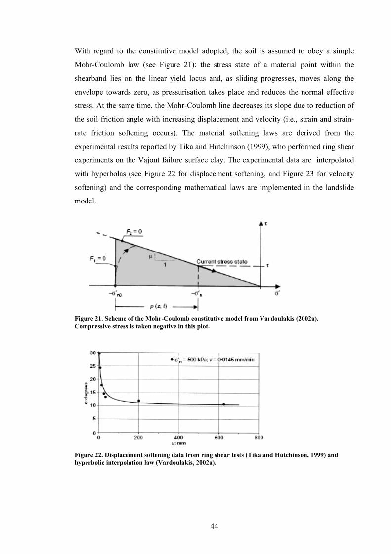
44

With regard to the constitutive model adopted, the soil is assumed to obey a simple

Mohr-Coulomb law (see Figure 21): the stress state of a material point within the

shearband lies on the linear yield locus and, as sliding progresses, moves along the

envelope towards zero, as pressurisation takes place and reduces the normal effective

stress. At the same time, the Mohr-Coulomb line decreases its slope due to reduction of

the soil friction angle with increasing displacement and velocity (i.e., strain and strain-

rate friction softening occurs). The material softening laws are derived from the

experimental results reported by Tika and Hutchinson (1999), who performed ring shear

experiments on the Vajont failure surface clay. The experimental data are interpolated

with hyperbolas (see Figure 22 for displacement softening, and Figure 23 for velocity

softening) and the corresponding mathematical laws are implemented in the landslide

model.

Figure 21. Scheme of the Mohr-Coulomb constitutive model from Vardoulakis (2002a). Compressive stress is taken negative in this plot.

Figure 22. Displacement softening data from ring shear tests (Tika and Hutchinson, 1999) and hyperbolic interpolation law (Vardoulakis, 2002a).

45

Figure 23. Velocity softening data from ring shear tests (Tika and Hutchinson, 1999) and hyperbolic interpolation law (Vardoulakis, 2002a).

2.3.4.1. The shearband equations

The first model equation, derived by Vardoulakis (2000) from the local form of the

energy balance law within the shearband, describes the 1-D time evolution of

temperature θ within the shearband:

( )2

02

ˆ ,( )n

mm

uk

t z j Cσ γθ θ μ γ γ

ρ′ −∂ ∂

= +∂ ∂

. (2.1)

The first term on the right-hand side is a heat diffusion term, where km is a constant

diffusivity coefficient, and the second one is a heat generation term, where

( ) 0ˆ , n u Dμ γ γ σ γ′ − = is the dissipation term, taken equal to the plastic work.

Dissipation depends on the plastic shear strain rate γ (conditions of simple shear inside

the shearband are assumed), the initial effective stress 0nσ ′ , the excess pore pressure u

and the strain- and strain rate-dependent friction coefficient μ̂ . The expression 0n uσ ′ −

reflects the effective stress principle: any generated excess pore pressures need to be

subtracted from 0nσ ′ , the initial vertical effective stress (i.e., the effective stress acting

on the shearband in static conditions). Finally, ( )m fj C Cρ = is a thermal constant that

derives from the energy balance (Vardoulakis, 2000), where j is the mechanical

equivalent of heat, ( )mCρ the product of the density and the specific heat of the soil-

water mixture.

The second equation describes the time evolution of excess pore pressure u generated

within the shearband:

v mu uct z z t

θλ∂ ∂ ∂ ∂⎛ ⎞= +⎜ ⎟∂ ∂ ∂ ∂⎝ ⎠. (2.2)

46

The first term on the right-hand side is a diffusion term, where cv is a temperature-

dependent consolidation coefficient. If this was the only nonzero term on the right hand

side, Equation (2.2) would correspond to a classic one-dimensional consolidation

equation (e.g. see Powrie, 1997) describing the dissipation of excess pore water

pressures in a porous medium. The second term describes pore pressure generation,

which depends on the heat produced, thus providing the cause of the occurrence of

excess pore pressures. The term λm is the temperature- and pore pressure-dependent

pressurisation coefficient (cf. sections 2.3.3 and 5.3.2), equal to the ratio between the

thermoplastic contraction coefficient and the compressibility of the soil. Coefficient λm

is set to zero until the temperature reaches the critical value for thermal collapse of the

soil skeleton, which in turn is determined from experimental data collected by Sultan

(1997). The determination of pressurisation coefficient nevertheless remains for the

author rather uncertain, due to a lack of direct experimental data (Vardoulakis, 2002a).

The third equation, derived from momentum balance inside the shear band, describes

the velocity profile therein:

( )2

0 2

1 ˆ , nv u vH ut z z

μ γ γ σρ⎡ ⎤⎛ ⎞∂ ∂ ∂′= − + −⎢ ⎥⎜ ⎟∂ ∂ ∂⎝ ⎠⎣ ⎦

, (2.3)

where ˆ

H μγ∂

=∂

is the “frictional rate sensitivity”. Since the structure of this equation

would lead to mathematical ill-posedness in the case H≤0 (Vardoulakis, 2001 and

2002a), a “second-gradient regularisation” (Vardoulakis and Sulem, 1995) of the

softening law was applied, leading to express (2.3) as a function of the fourth-order

spatial derivative of velocity. On the other hand, since after integration of the

momentum equation the resulting spatial profile of velocity within the shearband is very

close to a linear one (Vardoulakis 2001), the author suggests that a “linear

approximation” for the shearband velocity could be adopted instead of Equation (2.3).

This enables us to replace (2.3) with the expression

( )dzv v td

= (2.4)

(Vardoulakis 2000), where z is the coordinate defining the spatial position along the

domain thickness, d the (imposed) shearband thickness and ( )dv t is the time evolution

law for the velocity of the landslide, which coincides with the shearband velocity at its

upper boundary (cf. Figure 20). The governing equations for the shearband are therefore

reduced to the first two, and (2.4) can be expressed in function of the landslide velocity,

47

as soon as we proceed to consider the second sub-structure, constituted by the landslide

overburden.

2.3.4.2. The dynamical equation

Vardoulakis (2002a) presented a dynamic slip-circle analysis in order to apply the above

shearband model to the case history of Vajont, of which many field data are available

(Muller, 1964, Hendron and Patton, 1985, Tikka and Hutchinson 1999). Assuming a

rigid-body rotational failure mechanism, as can be seen from the drawings of ‘section

5’ of the Vajont slide (cf. Hendron and Patton, 1985 and Figure 20), the dynamical

equation is obtained from the moment balance of the involved driving and resisting

forces:

( ) ( )( )

20

ddm

c m

u tdv R Adt p

ω μμ

⎛ ⎞= +⎜ ⎟⎜ ⎟

⎝ ⎠ (2.5)

where 0ω is a constant depending on the landslide geometry, A and pc two functions of

both the mobilised friction coefficient and the friction coefficient for incipient failure

for the considered critical failure circle. The variable du is the excess pore pressure at

z d= , i.e. at the shearband-rigid block interface, whose evolution law is described by

Equation (2.2). Equation (2.5) was derived with the fundamental assumption that the

normal effective stress is constant along the whole failure circle, and set equal to a mean

value.

2.3.4.3. The landslide equations

The above governing equations form a system whose solution yields the time evolution

of temperature, pore pressure and slide velocity:

( )

( ) ( )

( ) ( )

2

2

20

,(I)

(II) ,

(III)

mf

v m

d dm

c m

D uk

t z C

u uc ut z z t

dv uR Adt p

γθ θ

θθ λ θ

ω μμ

⎧ ∂ ∂= +⎪

∂ ∂⎪⎪ ∂ ∂ ∂ ∂⎪ ⎛ ⎞= +⎨ ⎜ ⎟∂ ∂ ∂ ∂⎝ ⎠⎪⎪ ⎛ ⎞⎪ = +⎜ ⎟⎜ ⎟⎪ ⎝ ⎠⎩

. (2.6)

Several couplings (i.e. interdependencies between variables) appear in the above

equations: Equation (2.6)-(I) contains pore pressure-, displacement- and velocity-

dependency through the dissipation term, Equation (2.6)-(II) includes temperature-

dependency in the nonlinear coefficients and the second addend and Equation (2.6)-(III)

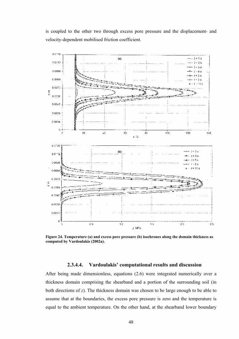
48

is coupled to the other two through excess pore pressure and the displacement- and

velocity-dependent mobilised friction coefficient.

(a)

(b)

Figure 24. Temperature (a) and excess pore pressure (b) isochrones along the domain thickness as computed by Vardoulakis (2002a).

2.3.4.4. Vardoulakis’ computational results and discussion

After being made dimensionless, equations (2.6) were integrated numerically over a

thickness domain comprising the shearband and a portion of the surrounding soil (in

both directions of z). The thickness domain was chosen to be large enough to be able to

assume that at the boundaries, the excess pore pressure is zero and the temperature is

equal to the ambient temperature. On the other hand, at the shearband lower boundary

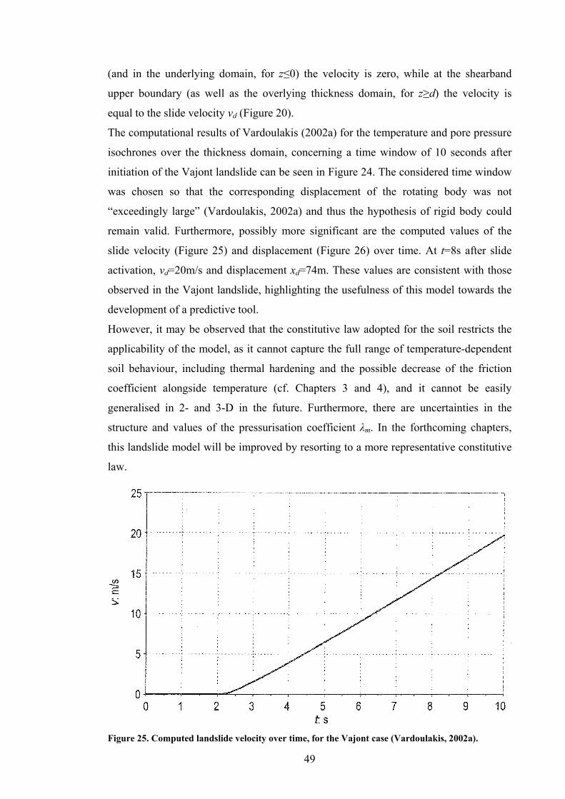
49

(and in the underlying domain, for z≤0) the velocity is zero, while at the shearband

upper boundary (as well as the overlying thickness domain, for z≥d) the velocity is

equal to the slide velocity vd (Figure 20).

The computational results of Vardoulakis (2002a) for the temperature and pore pressure

isochrones over the thickness domain, concerning a time window of 10 seconds after

initiation of the Vajont landslide can be seen in Figure 24. The considered time window

was chosen so that the corresponding displacement of the rotating body was not

“exceedingly large” (Vardoulakis, 2002a) and thus the hypothesis of rigid body could

remain valid. Furthermore, possibly more significant are the computed values of the

slide velocity (Figure 25) and displacement (Figure 26) over time. At t=8s after slide

activation, vd=20m/s and displacement xd=74m. These values are consistent with those

observed in the Vajont landslide, highlighting the usefulness of this model towards the

development of a predictive tool.

However, it may be observed that the constitutive law adopted for the soil restricts the

applicability of the model, as it cannot capture the full range of temperature-dependent

soil behaviour, including thermal hardening and the possible decrease of the friction

coefficient alongside temperature (cf. Chapters 3 and 4), and it cannot be easily

generalised in 2- and 3-D in the future. Furthermore, there are uncertainties in the

structure and values of the pressurisation coefficient λm. In the forthcoming chapters,

this landslide model will be improved by resorting to a more representative constitutive

law.

Figure 25. Computed landslide velocity over time, for the Vajont case (Vardoulakis, 2002a).

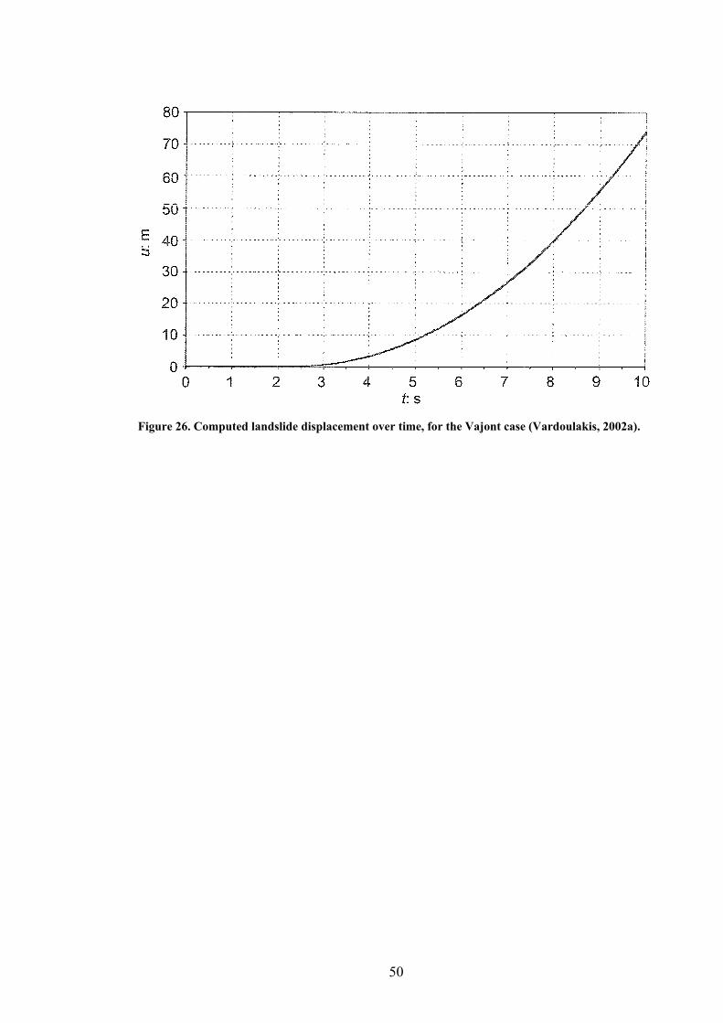
50

Figure 26. Computed landslide displacement over time, for the Vajont case (Vardoulakis, 2002a).

51

Chapter 3. Thermo-plasticity in clays. Review of existing models

3.1. The need for thermoplastic constitutive modelling

In Chapter 1, we have examined landslide case histories and existing models which

have been proposed in the literature to explain the unexpected loss in shear strength

observed in some catastrophic landslide cases. It emerged that a possible explanation to

these phenomena can be given by taking into account frictional heating and thermal

pressurisation. Vardoulakis (2002a) presented a comprehensive thermo-poro-

mechanical model, able to provide an effective back-analysis of the final collapse phase

of the Vajont slide. Nevertheless, the specialised constitutive law used for the soil

restricts the model’s applicability. In particular, it cannot capture the full range of

temperature-dependent soil behaviour observed experimentally, and it cannot be easily

generalised to two- or three-dimensional problems. In order to improve the model,

account should be taken for the temperature dependence of the mechanical behaviour of

soil, since whenever heat production is involved, different mechanisms may arise that

lead the soil-water mixture to alter its volumetric behaviour and show plastic yield in

unexpected conditions. As a first step towards the development of a more realistic

constitutive law, it is necessary to gather data and insight into the existing theories on

the thermoplastic behaviour of soils.

3.2. The ‘ingredients’ of soil elasto-plasticity

The main notions of soil elasto-plasticity are briefly recalled hereafter, for ease of

reference in the forthcoming sections.

The yield locus defines the combinations of mean effective stress and deviatoric stress

at which plastic yield begins to occur in the soil (e.g. see Muir Wood, 1990). When a

plastic loading state is attained, irrecoverable deformations develop (plastic flow

occurs), alongside a change in size of the yield curve itself. Consistently with the

Modified Cam-Clay theory (MCC) of Roscoe and Burland (1968), in isothermal

conditions the size of the yield locus

( )( ), , pc vf f p q′ ′= σ ε (3.1)

52

is a function of plastic volumetric strain through the ‘hardening relationship’, defining

the variation of apparent preconsolidation stress c′σ with volumetric strain pvε . When

plastic loading occurs, the elastic domain, enclosed within the yield surface, expands in

case of hardening, at positive (compactive) volumetric strain rates; and shrinks in case

of softening, at negative (dilative) volumetric strain rates. When temperature variations

θΔ occur, experimental evidence indicates that the elastic domain contracts with

0θΔ > and enlarges with 0θΔ < .

The generalisation of the Critical State model to introduce explicit dependency on

temperature consists of rewriting of the following classic “ingredients of elasto-

plasticity” (Muir Wood, 1990):

• Elasticity law, describing the recoverable deformations;

• Yield condition, describing the boundary of the stress region within which it is

possible to describe the deformation as elastic and recoverable;

• Hardening rule, describing the way in which the absolute magnitude of the

plastic deformation is linked with the changing size of the yield locus.

• Plastic potential (flow rule), to specify the relative magnitudes of various

components of plastic deformation that occurs when the soil is yielding.

3.3. Hueckel’s constitutive model

A thermo-elasto-plastic constitutive model for saturated soils was developed by

Hueckel and co-workers, based on experimental evidence, modification of the well-

known Critical State Soil Mechanics elasto-plastic theory (Roscoe and Schofield 1963,

Schofield and Wroth 1968, Roscoe and Burland 1968) and on Prager’s thermoplasticity

theory (Prager, 1958). The original model interprets the thermoplastic behaviour of the

soil skeleton and is used to describe drained failure (Hueckel and Baldi, 1990 and

Hueckel and Borsetto, 1990), while a second model for thermal volume change of pore

water (Baldi et al., 1988, Hueckel and Pellegrini, 1991) is used in combination with the

former to interpret undrained failure.

Hueckel’s model is described hereafter in terms of the four components of elasto-

plasticity described in Section 3.2.

53

3.3.1. Thermoelasticity

It has been experimentally shown (Hueckel and Peano, 1987), mainly from carrying out

temperature-controlled triaxial tests, that elastic thermal expansion tends to occur at low

effective confining stress (i.e., mainly in overconsolidated samples), and elasto-plastic

thermal compaction tends to occur at higher effective confining stress (i.e., mainly in

normally-consolidated samples).

Thermoelastic volumetric strains, tevε , in thermal conditions at constant isotropic stress,

are non-linearly dependent on the mean effective stress p’ and the temperature θ .

The thermoelastic deviatoric strain, teqε , is on the contrary purely mechanical (despite its

name, due to reasons of consistency of notation in a model that accounts for temperature

effects), and proportional to deviatoric stress. The elastic constitutive laws, expressed in

‘triaxial’ notation (i.e., in terms of isotropic and deviatoric stress), are

0 0

ln1

tev

K pe p

θ′

ε = −αΔ′+

(3.2)

( )01

3teq q q

Gε = − (3.3)

where:

3'2'

' 31 σσ +=p

'' 31 σσ −=q

K = bulk modulus at reference temperature,

G = shear modulus at reference temperature,

p0’, q0 = values of p’ and q at initial state,

α = coefficient of thermal expansion of clay, which includes the coefficient of

expansion of the clay solid mineral and that of porous skeleton, for an overall

dependency on four coefficients of “thermoplastic sensitivity” (Hueckel and Pellegrini,

1991).

3.3.2. Yield surface

The elliptical yield locus, derived from that of MCC, is expressed as:

( ) ( )

22

22 41 1

, ,tp tp

c v c v

p qfMθ θ

⎛ ⎞′⎜ ⎟= − + −⎜ ⎟′σ ε Δ ⎡ ⎤′σ ε Δ⎝ ⎠ ⎣ ⎦

(3.4)

54

In the above, the change in size of the yield surface is expressed through the change of

the temperature-dependent apparent preconsolidation stress c′σ , i.e. by the hardening

rule. The critical state parameter M is here considered to be independent of temperature.

3.3.3. Hardening relationship

The evolution law of the apparent preconsolidation isotropic stress is given by

( ) ( ) 21 0 1 2

12 exp 1 signtpc v

T

a e e a aK

θ θ θ⎛ ⎞⎧ ⎫

′ ⎡ ⎤σ = + + ε + Δ + Δ Δ⎜ ⎟⎨ ⎬⎣ ⎦⎜ ⎟λ −⎩ ⎭⎝ ⎠ (3.5)

where:

( )1 301T

KKe

θ θ= + α +α Δ Δ+

is a temperature dependent bulk modulus,

λ is the slope of the isotropic normal-compression line,

a = coefficient with the dimensions of a pressure,

e0, e1 = reference void ratio values,

a1, a2 = coefficients of thermal sensitivity of the yield surface.

3.3.4. Flow rule

The flow rule defines the mode of plastic deformation through the plastic potential

function, which specifies the relative magnitudes of shear and volumetric strain. Both

elastic and plastic strains occur at yielding, and their rates follow the additivity principle

(Hueckel and Pellegrini, 1991):

te tp

v v vte tp

q q q

ε ε ε

ε ε ε

= +

= + (3.6)

In general plasticity, the flow rule has the form p gλ ∂ε =∂σ

, where pε is the plastic strain

rate, g the plastic potential, σ the stress tensor and λ the scalar-valued plastic

multiplier, whose expression needs to be determined by the conditions which exist when

plastic loading continues (Section 3.3.5).

Hueckel and Borsetto (1990) proposed a non-associative flow rule, consisting of a

single plastic potential function g, but two distinct plastic multipliers, a ‘volumetric’

one, vλ , and a ‘deviatoric’ one, qλ so that:

tpv v

gp

ε λ ∂=

′∂ (3.7)

55

tpq q

gq

ε λ ∂=

∂ (3.8)

where the multipliers, postulated by to be positive at plastic yielding and zero otherwise,

are functions of the stress and temperature rates.

3.3.5. Consistency condition and plastic multiplier

The multiplier vλ is obtained through the so-called consistency condition. This equation

expresses an important postulate of theoretical plasticity, stating that if a stress

increment causes plastic loading and a corresponding change of plastic volumetric

strains, it must lie again on the new updated yield surface, which obeys the yield locus

equation expressed now in terms of the updated values of stress and plastic strain.

Analytically, the consistency condition can be expressed as

0tpvtp

v

f f f ff p qp q

θ εθ ε

∂ ∂ ∂ ∂′= + + + =′∂ ∂ ∂ ∂

(3.9)

(Hueckel and Borsetto, 1990), where f is the yield locus expressed in this case by (3.4).

The plastic multiplier can be calculated by substituting (3.7) in the above (3.9), thus

obtaining

v

f f fq pq p

H

θθλ

∂ ∂ ∂+ +

∂ ∂ ∂= (3.10)

where the ‘hardening modulus’ H has expression

pv

f gHpε

∂ ∂= −

′∂ ∂. (3.11)

Experimental observations led the authors to decide a different general form for the

multiplier Λq, which reflects the “deviation of thermoplastic strain rate from the normal

to mechanical plastic potential” (Hueckel and Borsetto, 1990):

1q v

fH

λ λ θ= + (3.12)

where f1 is a function of stress, temperature and plastic strain.

3.3.6. Loading/unloading and hardening/softening conditions

To complete the description of their constitutive model, Hueckel and Borsetto (1990)

specified the loading and unloading criteria, as these will differ from classic

‘isothermal’ plasticity due to the presence of temperature as an additional variable

featuring in the yield locus expression.

56

The condition of elastic unloading requires that 0f < , or 0f = and

0f f fq pq p

θθ

∂ ∂ ∂′+ + <′∂ ∂ ∂

(or equivalently, 0f < from the consistency condition (3.9),

since at elastic states 0tpvε = ), at 0vλ = .

Plastic loading, instead, requires 0f = and 0tpvtp

v

f f f ff p qp q

θ εθ ε

∂ ∂ ∂ ∂′= + + + =′∂ ∂ ∂ ∂

, at

0vλ > . At plastic loading we can have the two cases of hardening (increase of elastic

domain) and softening (decrease of elastic domain).

The condition of hardening is

0f f fq pq p

θθ

∂ ∂ ∂′+ + >′∂ ∂ ∂

, at 0H > , 0'>

∂∂pg

while the condition for softening is

0f f fq pq p

θθ

∂ ∂ ∂′+ + <′∂ ∂ ∂

, at 0H < , 0'<

∂∂pg .

It can be seen above that the same condition, 0f f fq pq p

θθ

∂ ∂ ∂′+ + <′∂ ∂ ∂

, represents both

the situation of elastic unloading and that of thermoplastic loading at softening. To

distinguish between the two cases, it is sufficient to look at the plastic multiplier vλ and

check whether this is positive or zero, as specified in the conditions above.

We observe that in order to gain a better understanding of the relationship between the

sign of the expression f f fp q pq p

θθ

⎛ ⎞∂ ∂ ∂′= + +⎜ ⎟′∂ ∂ ∂⎝ ⎠ and the loading/unloading condition,

it is perhaps more convenient to look at its geometrical meaning. The sign of p

determines the direction of the ‘stress-temperature rate’ vector ( ), ,p q θ′ by revealing

the angle formed between the direction of loading increment and the normal to the yield

surface. In fact, in contrast with isothermal plasticity, the yield function now depends on

three variables ( ), ,p q θ′ and may be visualised in three dimensions. In this framework,

0p > is the mathematical condition for which the stress-temperature rate vector points

outside the yield locus, while the condition 0p < means an inward orientation of the

stress-temperature rate vector with respect to the yield surface. We can now understand

why in thermal plasticity the distinction between hardening and softening cannot be

uniquely defined by the orientation of the two-dimensional ‘stress rate’ vector ( ',p q )

57

(Hueckel and Borsetto 1990): the stress rate vector ( ),p q′ is no other than the

projection of the stress-temperature rate vector ( ), ,p q θ′ into the ( )',p q plane. Thus,

the stress rate vector (in two dimensions) can point inwards at hardening, while the

stress-temperature rate vector (in three dimensions) still points outwards. As an

example, in Figure 27 this situation is visualized in three dimensions, where the

modified Cam-Clay ellipse shrinking with increasing temperature describes a ‘saddle-

shaped’ function in (p,q,θ) space. A sample stress-temperature increment vector

( )v , ,p q θ′Δ = Δ Δ Δ has been drawn in Figure 27, which can be shown to represent a

case of hardening by projecting it both in the (q, θ) plane (2-D section at p’=constant)

and in the ( )',p q plane (2-D section at θ=constant), in Figure 28: despite its projection

on the ( )',p q plane points inwards, the ( ),q θ projection reveals that the stress-

temperature rate vector ( ), ,p q θ′ actually points outwards.

The above depicted situation is illustrated analytically by Hueckel and Borsetto (1990),

together with the opposite and symmetric situation of having an outward stress rate at

softening.

p’

q

p’

q

p’

q

θ

θ0

θ 1> θ 0

θ 2> θ 1

Δv

Figure 27. Sample thermo-plastic yield locus in three dimensions, with sample stress-temperature rate vector Δv.

58

Δv

Δθ>0

Δq<0

p’

q

Δq<0Δv

Δp’<0

θ

q

θ0 θ1 θ2

p’=p1’

θ=θ1

p1’

Figure 28. Projections of the stress-temperature rate vector Δv (Figure 27) on the deviatoric stress vs. temperature plane and on the deviatoric stress vs. mean effective stress plane.

3.3.7. Associative flow rule

Despite the non-associative flow rule assumed in the formulation of the constitutive

model by Hueckel and Borsetto (1990), and despite the experimental evidence of some

non-associative behaviour (Hueckel and Baldi, 1990), the model adopted by the authors

for carrying out numerical simulations (Hueckel and Pellegrini, 1991) is associative.

Furthermore, to our knowledge no explicit formulation is given for the plastic potential

g in any of the authors’ publications on the subject. Adopted for simplicity, the

associative rule prescribes that the yield and plastic potential functions coincide, i.e.

g f= , and also v qλ λ= . The flow rule (Section 3.3.4) may be thus simplified as

tpv

tpq

fpfq

ε λ

ε λ

∂=

′∂∂

=∂

(3.13)

59

where λ is expressed in the same way as vλ in Equation (3.10).

3.4. Laloui’s constitutive model

3.4.1. Introduction

The second thermoplastic model that we are going to review was developed by Laloui et

al. (2002, 2005) and Laloui and Cekerevac (2003) and includes the description of an

isotropic and a deviatoric yield mechanism. Laloui and co-workers also proposed more

sophisticated cyclic thermoplastic and thermo-viscoplastic orthotropic models in order

to take soil anisotropy into account (Modaressi and Laloui 1997, Laloui 2001);

however, we will not extend our review to these models since treating anisotropic soils

is outside the scope of this work.

Laloui’s thermo-mechanical model, similarly to Hueckel’s model, mainly explores the

volumetric behaviour and the isotropic yield mechanism of clays subjected to

temperature changes. In a more recent paper, a theoretical formulation including a

separate deviatoric mechanism was added to complete the constitutive framework

(Laloui et al., 2005). Experiments were performed by the authors using a standard

triaxial apparatus, modified to enable temperature control. Laboratory tests involved

either thermal loading of clay samples at constant confining stress, or isothermal

isotropic compression tests carried out at different (constant) temperatures.

The structure of this model is similar to that of Hueckel’s model, but appears simpler in

that it involves fewer material parameters and the yield locus is assumed to coincide

with the plastic potential (associative flow rule). On the other hand, the authors resort to

concepts from the theory of ‘multi-mechanism plasticity’ (Koiter 1960, Mandel 1965)

to formulate the equations describing the deviatoric thermoplastic behaviour, resulting

in the need for two separate plastic multipliers, despite the assumption of associative

flow rule.

The total strain rate tensor due to thermo-mechanical loading is composed of a thermo-

elastic part, teε , and thermo-plastic part, tpε :

te tpij ij ijε ε ε= + . (3.14)

the elastic and plastic contributions to the total strain rate are discussed separately

hereafter.

60

3.4.2. Thermoelasticity

The volumetric thermoelastic strain rate is the sum of a reversible thermal strain and a

mechanical strain component:

tev s

pK

ε β θ′

= + (3.15)

where sβ is the elastic thermal expansion coefficient of the solid skeleton, which is

allowed to vary non-linearly with temperature and pressure (Laloui and Cekerevac,

2003). The elastic bulk modulus depends on the stress value according to

n

refref

pK Kp

⎛ ⎞′= ⎜ ⎟⎜ ⎟

⎝ ⎠ (3.16)

where n is a material constant.

The (purely mechanical) deviatoric elastic strain rate is written as

d

ed G

σε = (3.17)

where dσ is the deviatoric effective stress tensor, and the shear elastic modulus is given

by

n

refref

pG Gp

⎛ ⎞′= ⎜ ⎟⎜ ⎟

⎝ ⎠. (3.18)

3.4.3. Multi-mechanism thermoplasticity

Laloui et al. (2005) propose to formally sub-divide their plastic framework into an

isotropic and a deviatoric mechanism, giving rise to two different flow relationships and

two consistency conditions. The total plastic strain rate is presented as the sum of two

partial strain rates:

2

, , ,1

tp tp tp tpij ij k ij iso ij dev

kε ε ε ε

=

= = +∑ (3.19)

(Laloui et al., 2005), where each strain rate occurs if the stress state reaches the

corresponding yield function. The isotropic yield surface fTi is identified with the curve

describing the temperature dependency of apparent preconsolidation stress in the ( ),p θ′

plane, while the deviatoric yield surface fTd coincides with the original Cam Clay (OCC)

yield envelope (Roscoe and Schofield, 1963) in the ( ),p q′ plane. In this multi-

mechanism framework, a general form of flow rule can be written as:

61

2

1

tp kij k

k ij

gε λσ=

∂=

′∂∑ (3.20)

where one plastic potential and one plastic multiplier per mechanism are employed.

The two yield functions can be represented together, in a 3-dimensional space in order

to define a closed domain representing the elastic region (Figure 32).

3.4.3.1. Isotropic yield mechanism and flow rule

The expression of the isotropic yield limit is

( ),pTi c vf p rσ ε θ′ ′= − (3.21)

(Laloui et al., 2005). In the above, cσ ′ is the apparent isotropic preconsolidation stress

and r represents the “degree of plastification” to account for “progressive evolution of

the yield limit during loading” (Laloui et al., 2005).

The apparent preconsolidation stress is expressed as a function of volumetric plastic

strain and temperature (Laloui and Cekerevac, 2003):

( ) ( ) ( )0 0 01 log exp pc c vσ σ θ γ θ θ βε′ ′= −⎡ ⎤⎣ ⎦ . (3.22)

In the above, ( )0 0cσ θ′ is the preconsolidation stress at reference temperature, γ is a

material parameter defining the rate of decrease of cσ ′ with θ and β is the plastic

compressibility modulus.

By substituting expression (3.22) into the yield locus expression, we obtain the final

form of the isotropic thermoplastic yield locus:

( ) ( ) ( )0 0 01 log exp pTi c vf p rσ θ γ θ θ βε′ ′= − −⎡ ⎤⎣ ⎦ . (3.23)

Laloui’s isotropic yield limit is represented in Figure 29 along with some experimental

data points. At the left of the curve, any stress or temperature change causes reversible

strains. As soon as the curve is attained by an increase in mean stress and/or

temperature, plastic strains occur.

The flow rule proposed by the authors is associated. The ‘isotropic contribution’ to the

total strain rate (Laloui et al., 2005) is:

p Ti Tiv i i i

g fp p

ε λ λ λ∂ ∂= = =

′ ′∂ ∂. (3.24)

3.4.3.2. Deviatoric yield mechanism and flow rule

The deviatoric yield surface proposed by Laloui et al. (2005) is based on the OCC yield

locus:

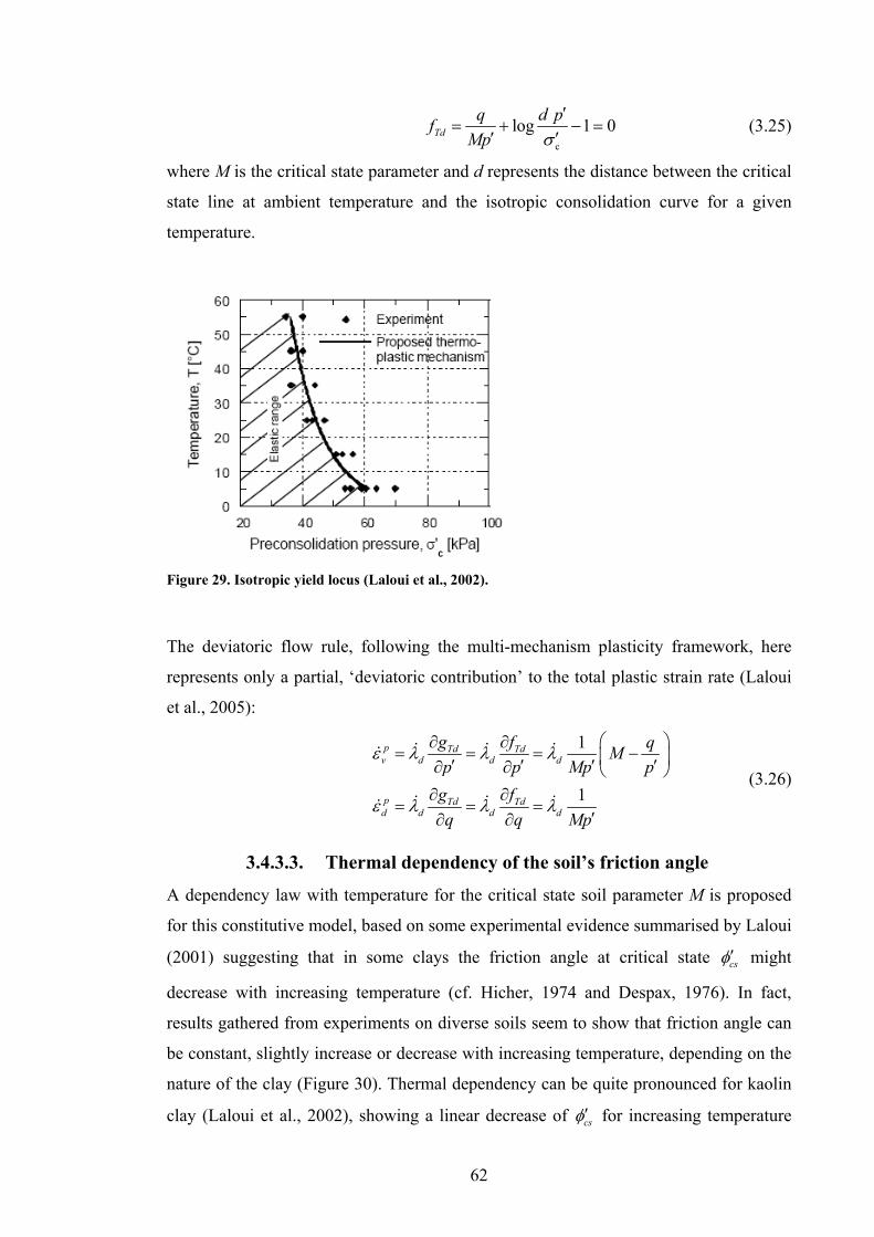
62

c

log 1 0Tdq d pf

Mp σ′

= + − =′ ′

(3.25)

where M is the critical state parameter and d represents the distance between the critical

state line at ambient temperature and the isotropic consolidation curve for a given

temperature.

Figure 29. Isotropic yield locus (Laloui et al., 2002).

The deviatoric flow rule, following the multi-mechanism plasticity framework, here

represents only a partial, ‘deviatoric contribution’ to the total plastic strain rate (Laloui

et al., 2005):

1

1

p Td Tdv d d d

p Td Tdd d d d

g f qMp p Mp p

g fq q Mp

ε λ λ λ

ε λ λ λ

⎛ ⎞∂ ∂= = = −⎜ ⎟′ ′ ′ ′∂ ∂ ⎝ ⎠

∂ ∂= = =

′∂ ∂

(3.26)

3.4.3.3. Thermal dependency of the soil’s friction angle

A dependency law with temperature for the critical state soil parameter M is proposed

for this constitutive model, based on some experimental evidence summarised by Laloui

(2001) suggesting that in some clays the friction angle at critical state csφ′ might

decrease with increasing temperature (cf. Hicher, 1974 and Despax, 1976). In fact,

results gathered from experiments on diverse soils seem to show that friction angle can

be constant, slightly increase or decrease with increasing temperature, depending on the

nature of the clay (Figure 30). Thermal dependency can be quite pronounced for kaolin

clay (Laloui et al., 2002), showing a linear decrease of csφ′ for increasing temperature

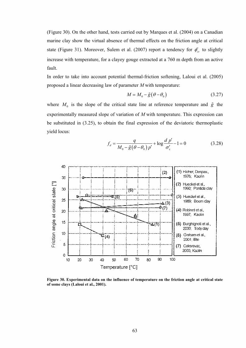
63

(Figure 30). On the other hand, tests carried out by Marques et al. (2004) on a Canadian

marine clay show the virtual absence of thermal effects on the friction angle at critical

state (Figure 31). Moreover, Sulem et al. (2007) report a tendency for csφ′ to slightly

increase with temperature, for a clayey gouge extracted at a 760 m depth from an active

fault.

In order to take into account potential thermal-friction softening, Laloui et al. (2005)

proposed a linear decreasing law of parameter M with temperature:

( )0 0M M g θ θ= − − (3.27)

where 0M is the slope of the critical state line at reference temperature and g the

experimentally measured slope of variation of M with temperature. This expression can

be substituted in (3.25), to obtain the final expression of the deviatoric thermoplastic

yield locus:

( )0 0 c

log 1 0dq d pf

M g pθ θ σ′

= + − =′ ′− −

(3.28)

Figure 30. Experimental data on the influence of temperature on the friction angle at critical state of some clays (Laloui et al., 2001).

64

3.4.3.4. Volumetric strain coupling and consistency conditions

The two above presented mechanisms are coupled through the hardening relationship

(3.22), since both yield loci depend on the apparent overconsolidation stress. The total

volumetric strain rate results from the sum of the two ‘partial’ contributions:

p Td Tiv d i

f fp p

ε λ λ∂ ∂= +

′ ′∂ ∂. (3.29)

It is finally worth mentioning the expressions of the consistency conditions, determined

by two distinct equations as required by the multi-mechanism approach, allowing us to

calculate the two plastic multipliers:

0pTi Ti Ti TiTi vp

v

f f f ff p rp r

θ εθ ε

∂ ∂ ∂ ∂′= + + + =′∂ ∂ ∂ ∂

(3.30)

0pTd Td Td TdTd vp

v

f f f ff p qp q

θ εθ ε

∂ ∂ ∂ ∂′= + + + =′∂ ∂ ∂ ∂

. (3.31)

As a summary of Laloui’s model, the coupled isotropic and deviatoric yield loci are

visualised a three-dimensional space in Figure 32.

Figure 31. From Marques et al. (2004). Temperature effect on the critical state line for the St-Roch-de-l’Achigan Canadian clay.

3.5. Other authors’ contributions to thermo-mechanical soil modelling

We are now going to briefly present two further constitutive thermo-mechanical models

which have been recently presented, both based on the modification of Hueckel’s

model, in an attempt to better represent the volumetric behaviour of soils, especially

focusing on the thermal behaviour of overconsolidated clays.

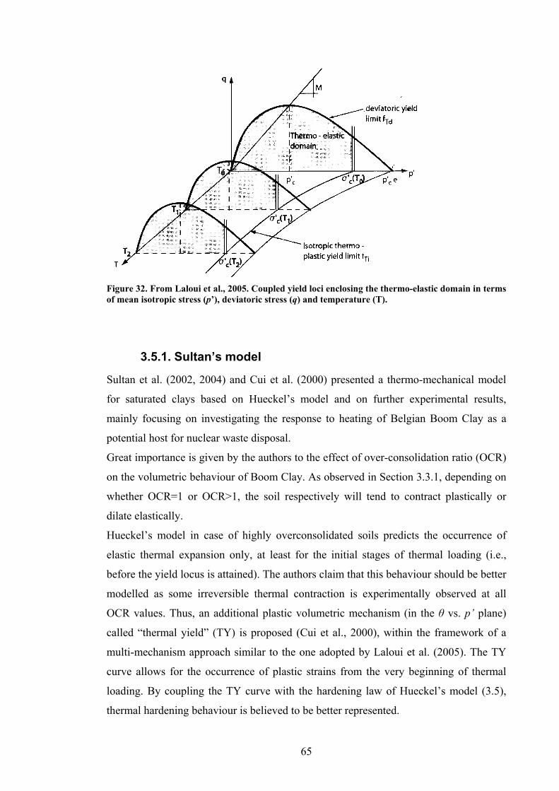
65

Figure 32. From Laloui et al., 2005. Coupled yield loci enclosing the thermo-elastic domain in terms of mean isotropic stress (p’), deviatoric stress (q) and temperature (T).

3.5.1. Sultan’s model

Sultan et al. (2002, 2004) and Cui et al. (2000) presented a thermo-mechanical model

for saturated clays based on Hueckel’s model and on further experimental results,

mainly focusing on investigating the response to heating of Belgian Boom Clay as a

potential host for nuclear waste disposal.

Great importance is given by the authors to the effect of over-consolidation ratio (OCR)

on the volumetric behaviour of Boom Clay. As observed in Section 3.3.1, depending on

whether OCR=1 or OCR>1, the soil respectively will tend to contract plastically or

dilate elastically.

Hueckel’s model in case of highly overconsolidated soils predicts the occurrence of

elastic thermal expansion only, at least for the initial stages of thermal loading (i.e.,

before the yield locus is attained). The authors claim that this behaviour should be better

modelled as some irreversible thermal contraction is experimentally observed at all

OCR values. Thus, an additional plastic volumetric mechanism (in the θ vs. p’ plane)

called “thermal yield” (TY) is proposed (Cui et al., 2000), within the framework of a

multi-mechanism approach similar to the one adopted by Laloui et al. (2005). The TY

curve allows for the occurrence of plastic strains from the very beginning of thermal

loading. By coupling the TY curve with the hardening law of Hueckel’s model (3.5),

thermal hardening behaviour is believed to be better represented.

66

Deviatoric effects, in analogy with Hueckel, are described by Cui et al. (2000) following

the Modified Cam-Clay framework, adopting an associated flow rule and assuming the

critical state friction parameter M as constant, due to the scarce availability of

experimental evidence able to show differently. The 3-D visualization of the yield locus

is shown in Figure 33.

3.5.2. Robinet’s model

Robinet et al. (1996) also proposed a modification of Hueckel’s model with the

introduction of a further thermo-plastic mechanism to better interpret thermal softening.

An additional isotropic yield surface is proposed, associated with a threshold

temperature, beyond which both reversible and irreversible thermal strains may develop.

Furthermore, a different hardening rule to those described so far is proposed, in the

form of product of two exponential functions, with the purpose of not allowing the yield

surface size to change at cooling (in contrast with Hueckel’s and Laloui’s models),

when the temperature is below a threshold value.

Regarding the deviatoric part, modified Cam-Clay is adopted, in analogy with the

models of Hueckel and Sultan. However, a non-associative flow rule is proposed here,

with the plastic potential implicitly dependent on temperature changes.

Figure 33. From Cui et al. (2000). Yield surface in 3 dimensions. On the temperature (T) vs. isotropic stress (p’) plane, TY represents the newly introduced thermal yield curve, while LY corresponds to Hueckel’s hardening law.

67

3.6. Discussion

The constitutive models reviewed in this chapter depict a fairly comprehensive view of

the thermo-mechanical behaviour of clays, and despite they have all been primarily

developed in the framework of nuclear waste disposal in deep geological formations, it

is reasonable to employ them in other fields, after the necessary modifications.

The first comprehensive thermo-mechanical model suitable for numerical

implementations was developed by Hueckel and co-workers. After them, Sultan,

Robinet and co-workers aimed to improve on the volumetric thermo-plastic mechanism

in response to specific problems arising in the context of nuclear waste repository

design, where the soil undergoes relatively slow temperature changes whilst remaining

at constant confining stress. Laloui and co-workers independently developed a thermo-

mechanical constitutive framework which appears simpler, yet able to realistically

describe the main features of the soil’s deformational response to heating.

Our aim is to incorporate one of the above described constitutive laws into the

governing equations of a model describing the production of heat and excess pore

pressure in a rapidly deforming shearband (Chapter 5). Given the extreme overall

complexity of such model, and the presence of some uncertainties in the determination

of its parameters, the thermo-plastic constitutive model for the soil should be as simple

as possible, i.e. it should contain the least possible number of material parameters and

should be easy to generalise. Among the above reviewed models, Laloui’s one appears

to be the most suitable for the purpose, since its formulation is simpler, there are fewer

material parameters and the elastic law can be easily inverted leading to a strain-

controlled problem, which will more easily allow future generalisations. Nevertheless,

the model will need modifications since adopting a multi-mechanism framework

implying the use of two separate plastic multipliers does not appear necessary to our

purposes, and the OCC yield locus is notoriously awkward for numerical

implementations as compared to MCC, due to the uncertainties in the direction of the

plastic strain increment vector at the tip of the yield envelope (e.g. see Muir Wood,

1990). Furthermore, the stress-strain formulation adopted by Laloui and co-workers is

the classic ‘triaxial’ one, which is appropriate to interpret triaxial testing, but not general

enough for other contexts and for potential Finite Element implementations.

In the next chapter, we will focus on improving and generalising Laloui’s model in

order to make it suitable for the implementation into a thermo-mechanical landslide

model.

68

Chapter 4. An improved thermo-mechanical constitutive model

4.1. Introduction

In this chapter a new generalised thermoplastic model is developed, based on the

isotropic hardening law describing the evolution of apparent preconsolidation stress

with temperature of Laloui & Cekerevac (2003) and adopting the linear thermal-friction

softening law of Laloui et al. (2005). With these ingredients we can re-derive the

constitutive equations from a standard plasticity framework, with a general stress space

formulation in order to facilitate future generalisation of the model in 2- and 3-D.

Furthermore Modified Cam-Clay will be adopted for the deviatoric behaviour, as this is

a widely used model with clear advantages when it comes to numerical implementation

(cf. Section 3.6). The resulting qualitative shape of the yield surface in 3 dimensions is

shown in Figure 34. It can be noticed that the tip of the yield locus, i.e. the apparent

preconsolidation stress, varies with temperature in the (p’,θ) plane (cf. Section 3.4.3.1)

according to the following exponential law (Laloui & Cekerevac 2003):

( )0 0exp( ) 1 logpc c vσ σ βε γ θ θ′ ′= −⎡ ⎤⎣ ⎦ (4.1)

At the same time, if the considered soil shows some thermal-friction sensitivity (i.e.

0g ≠ , cf. Section 3.4.3.3), the critical state parameter M may linearly vary as (Laloui et

al., 2005)

( )0 0M M g θ θ= − − . (4.2)

Starting from a classic plasticity formulation, we will hereafter derive the stress-strain

rate equations including the above thermo-mechanical laws in the framework of

Modified Cam Clay (MCC).

4.2. Problem formulation

Within the range of small deformations and rotations, from standard kinematics we can

assume the validity of additive decomposition of total strain into elastic and plastic part,

as well as the corresponding decomposition of their rates:

e p= +ε ε ε (4.3)

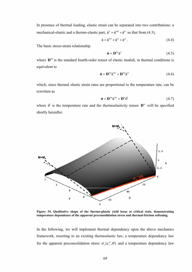
69

In presence of thermal loading, elastic strain can be separated into two contributions: a

mechanical-elastic and a thermo-elastic part, e me te= +ε ε ε so that from (4.3),

me te p= + +ε ε ε ε . (4.4) The basic stress-strain relationship

me e=σ D ε (4.5)

where meD is the standard fourth-order tensor of elastic moduli, in thermal conditions is

equivalent to

me me me te= +σ D ε D ε (4.6) which, since thermal elastic strain rates are proportional to the temperature rate, can be

rewritten as

me me teθ= +σ D ε D (4.7)

where θ is the temperature rate and the thermoelasticity tensor teD will be specified

shortly hereafter.

M=M0

M=Mθ

σc’ (θ)

Figure 34. Qualitative shape of the thermo-plastic yield locus at critical state, demonstrating temperature dependence of the apparent preconsolidation stress and thermal-friction softening.

In the following, we will implement thermal dependency upon the above mechanics

framework, resorting to an existing thermoelastic law, a temperature dependency law

for the apparent preconsolidation stress ( , )pc vσ ε θ and a temperature dependency law

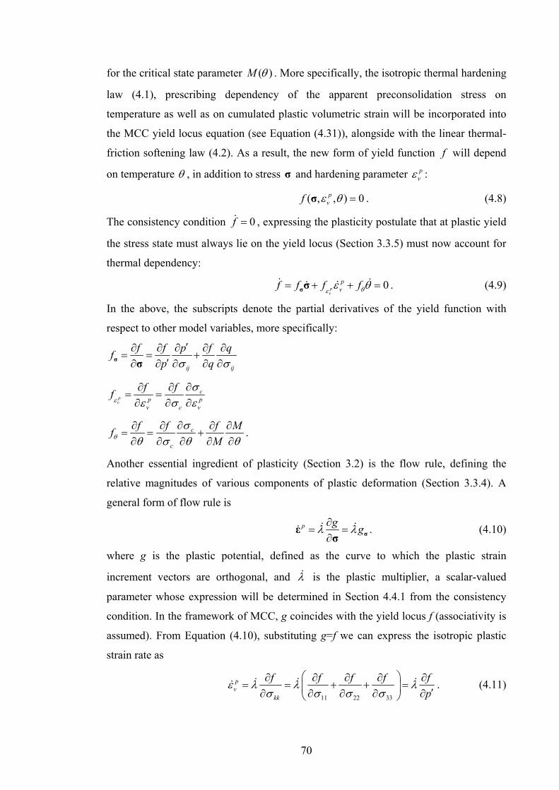
70

for the critical state parameter ( )M θ . More specifically, the isotropic thermal hardening

law (4.1), prescribing dependency of the apparent preconsolidation stress on

temperature as well as on cumulated plastic volumetric strain will be incorporated into

the MCC yield locus equation (see Equation (4.31)), alongside with the linear thermal-

friction softening law (4.2). As a result, the new form of yield function f will depend

on temperature θ , in addition to stress σ and hardening parameter pvε :

( , , ) 0pvf ε θ =σ . (4.8)

The consistency condition 0f = , expressing the plasticity postulate that at plastic yield

the stress state must always lie on the yield locus (Section 3.3.5) must now account for

thermal dependency:

0pv

pvf f f fθεε θ= + + =σσ . (4.9)

In the above, the subscripts denote the partial derivatives of the yield function with

respect to other model variables, more specifically:

ij ij

f f p f qfp qσ σ

′∂ ∂ ∂ ∂ ∂= = +

′∂ ∂ ∂ ∂ ∂σ σ

pv

cp p

v c v

f ffε

σε σ ε

∂∂ ∂= =∂ ∂ ∂

c

c

f f f MfMθ

σθ σ θ θ

∂∂ ∂ ∂ ∂= = +∂ ∂ ∂ ∂ ∂

.

Another essential ingredient of plasticity (Section 3.2) is the flow rule, defining the

relative magnitudes of various components of plastic deformation (Section 3.3.4). A

general form of flow rule is

p g gλ λ∂= =

∂ σεσ

. (4.10)

where g is the plastic potential, defined as the curve to which the plastic strain

increment vectors are orthogonal, and λ is the plastic multiplier, a scalar-valued

parameter whose expression will be determined in Section 4.4.1 from the consistency

condition. In the framework of MCC, g coincides with the yield locus f (associativity is

assumed). From Equation (4.10), substituting g=f we can express the isotropic plastic

strain rate as

11 22 33

pv

kk

f f f f fp

ε λ λ λσ σ σ σ

⎛ ⎞∂ ∂ ∂ ∂ ∂= = + + =⎜ ⎟ ′∂ ∂ ∂ ∂ ∂⎝ ⎠

. (4.11)

71

Based on the above outlined framework, we will now derive the equations of the

thermo-elasto-plastic model. It is necessary to start the description from the constitutive

law of elasticity, which forms the basis of all stress-strain relationships, to which a

description of plasticity will follow. In fact, elastic (i.e., recoverable) strains are always

present when soil is deformed, while plastic (i.e., irrecoverable) strains occur only if the

yield locus is attained by the stress state.

4.3. Thermoelasticity

The thermoelastic relationships imply recoverable volumetric dilation with increased

temperature, and can be obtained from standard continuum mechanics (e.g. Mase, 1970,

Section 6.10). The strain rate components of an isotropic body subjected to thermal

loading are expressed by

teijα θ=ε δ (4.12)

where α is the thermal elastic expansion coefficient and ijδ is the Kronecker delta, a

function of the variables i,j defined as

1 for 0 for ij

i ji j

δ=⎧

= ⎨ ≠⎩ (4.13)

which practically, in Equation (4.12) zeroes all the deviatoric components of strain.

Adding up the mechanical-elastic part (standard Hooke’s law) yields the so-called

Duhamel-Neumann relations, which in turn can be inverted to give the thermoelastic

constitutive equations:

( )2 3 2me meij kk ij ijλ μ λ μ α θ= + − +σ δ ε ε δ (4.14)

where λ and μ are the Lamè constants (Mase, 1970).

On the other hand, Laloui et al. (2005) provided the thermoelastic relations

tev sε β θ= ; (4.15)

in terms of volumetric strain, which can be equivalently written in vector form as

te Teθ=ε C (4.16)

where 13

Tes ijβ=C δ . By comparing (4.12) and (4.16) we deduce

13 sα β= , (4.17)

which allows us to write, from (4.15),

3tevε αθ= . (4.18)

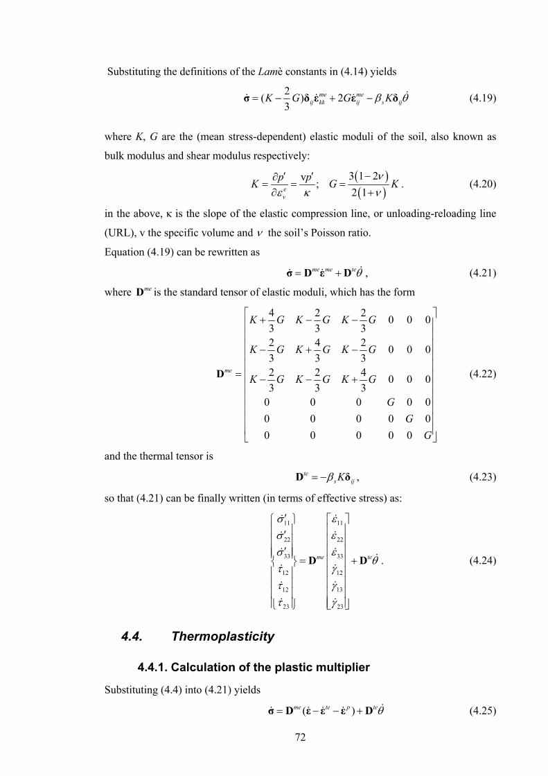
72

Substituting the definitions of the Lamè constants in (4.14) yields

2( ) 23

me meij kk ij s ijK G G Kβ θ= − + −σ δ ε ε δ (4.19)

where K, G are the (mean stress-dependent) elastic moduli of the soil, also known as

bulk modulus and shear modulus respectively:

( )( )

3 1 2v ; 2 1e

v

p pK G Kν

ε κ ν−′ ′∂

= = =∂ +

. (4.20)

in the above, κ is the slope of the elastic compression line, or unloading-reloading line

(URL), v the specific volume and ν the soil’s Poisson ratio.

Equation (4.19) can be rewritten as

me me teθ= +σ D ε D , (4.21)

where meD is the standard tensor of elastic moduli, which has the form

4 2 2 0 0 03 3 32 4 2 0 0 03 3 32 2 4 0 0 03 3 3

0 0 0 0 00 0 0 0 00 0 0 0 0

me

K G K G K G

K G K G K G

K G K G K G

GG

G

⎡ ⎤+ − −⎢ ⎥⎢ ⎥⎢ ⎥− + −⎢ ⎥⎢ ⎥

= ⎢ ⎥− − +⎢ ⎥⎢ ⎥⎢ ⎥⎢ ⎥⎢ ⎥⎣ ⎦

D (4.22)

and the thermal tensor is

tes ijKβ= −D δ , (4.23)

so that (4.21) can be finally written (in terms of effective stress) as:

1111

2222

3333

1212

1312

23 23

me te

εσεσεσ

θγτγτ

τ γ

′ ⎡ ⎤⎧ ⎫⎢ ⎥⎪ ⎪′ ⎢ ⎥⎪ ⎪

′ ⎢ ⎥⎪ ⎪⎪ ⎪ = +⎢ ⎥⎨ ⎬⎢ ⎥⎪ ⎪⎢ ⎥⎪ ⎪⎢ ⎥⎪ ⎪⎢ ⎥⎪ ⎪⎩ ⎭ ⎣ ⎦

D D . (4.24)

4.4. Thermoplasticity

4.4.1. Calculation of the plastic multiplier

Substituting (4.4) into (4.21) yields

( )me te p teθ= − − +σ D ε ε ε D (4.25)

73

or equivalently, by substituting (4.10) and (4.16),

( )me me te te me gθ λ= − − − σσ D ε D C D D . (4.26)

Equation (4.26) can be substituted into the consistency Equation (4.9)

( ) 0pv

me me te te mepf f f g f g fθε

θ λ λ θ− − − + + =σ σ σ σD ε D C D D . (4.27)

Solving this equation for the plastic multiplier yields

( )

pv

me me te te

mep

f f f ff g f g

θ

ε

θλ

′

+ − +=

−σ σ σ

σ σ

D ε D C DD

. (4.28)

In the above, expression me te tef f− +σ σD C D can be algebraically manipulated as:

( )

( )

13

1 2 23 3

1 3 2 23

2 2

te me te te mes kl

tes ij kk ij

s ij s ij

tes ij

f f

f K G G

f K K G G

K f f

β

β

β β

β

⎛ ⎞− = −⎜ ⎟⎝ ⎠

⎧ ⎫⎡ ⎤⎛ ⎞= − − + =⎨ ⎬⎜ ⎟⎢ ⎥⎝ ⎠⎣ ⎦⎩ ⎭⎡ ⎤= − − − + =⎢ ⎥⎣ ⎦

= − =

σ σ

σ

σ

σ σ

D D C D D δ

D δ δ δ

δ δ

δ D

(4.29)

which leads to the final expression:

( ) ( )

2 1 2pv

me teme te

mep

f f ff f f

f g f g Hθ

θε

θλ θ

′

+ +⎡ ⎤= = + +⎣ ⎦−

σ σσ σ

σ σ

D ε DD ε D

D. (4.30)

We may recall here that the MCC yield surface has expression

( )2 2cf q M p pσ′ ′ ′= − − (4.31)

and its derivatives, featuring in Equation (4.30), are described in Section 4.2. In thermal

conditions, we may employ expression (4.1) to describe thermal dependency of the

preconsolidation stress. The critical state parameter M may be allowed to vary

according to the linear thermal-friction softening law (4.2). Substituting equations (4.2)

and (4.1) into (4.31) yields

( ) ( )220 0 0

0

exp 1 logpc vf q M g p pθθ θ σ βε γ

θ

⎧ ⎫⎡ ⎤⎛ ⎞⎪ ⎪′ ′ ′= − − − − −⎡ ⎤ ⎨ ⎬⎢ ⎥⎜ ⎟⎣ ⎦⎝ ⎠⎪ ⎪⎣ ⎦⎩ ⎭

. (4.32)

The partial derivatives of the yield function outlined in Section 4.2 can finally be

calculated, as follows:

74

( ) ( ) ( ){ }( ) ( )

( ) ( ){ }

20 0

0 0 0

20 0 0

20 0 0

2 1 log

1 log

2 1 log

2

pv

mm

m

p p m

q

p M gf gp M g p

f p M g

f g M g p

f q

θ

ε

σ λ θ θθ θ σ γ θ θ

θ

σ β γ θ θ θ θ

θ θ σ γ θ θ′ ′

′ ′ − −⎡ ⎤⎣ ⎦ ′ ′ ′= + − − − −⎡ ⎤ ⎡ ⎤⎣ ⎦ ⎣ ⎦

′ ′= − − − −⎡ ⎤ ⎡ ⎤⎣ ⎦ ⎣ ⎦

′ ′= = − − − −⎡ ⎤ ⎡ ⎤⎣ ⎦ ⎣ ⎦=

(4.33)

In the above equations,

( )0 exp pm c vσ σ βε′ ′= (4.34)

is the ‘isothermal’ value of apparent preconsolidation stress (Laloui and Cekerevac

2003). Equation (4.34) corresponds to the classic MCC hardening law, where thermal

loading is not expected and preconsolidation stress depends on the volumetric plastic

strains developed during the loading history of the considered soil.

4.4.2. Thermo-elasto-plastic stress-strain rate equations

Employing (4.4) into (4.7) yields

( )me te p teθ= − − +σ D ε ε ε D (4.35)

which, by substituting (4.16) leads to

( ) ( )me p te te me θ= − + −σ D ε ε D C D . (4.36)

Substituting (4.10) and (4.30) yields

( ) ( )1 2me me te te te meTf f f g

Hθ θ⎧ ⎫⎡ ⎤= − + + + −⎨ ⎬⎣ ⎦⎩ ⎭

σ σ σσ D ε D ε D D C D (4.37)

By regrouping the terms, the above becomes

( )e me te te me mep tepgλ θ θ= − + − = +σσ σ D D C D D ε D (4.38)

which represents the stress-strain rate equation in the general case of thermo-mechanical

loading.

4.4.3. Hardening law and final thermoplastic equations

The hardening rule describes the way in which plastic deformation is linked with the

change in size of the yield locus, through the value of apparent preconsolidation stress

located at the ‘tip’ of the envelope (i.e. at the intersection of the yield locus with the

isotropic axis), according to modified Cam Clay (e.g. see Muir Wood, 1990). The MCC

hardening law (not accounting for thermal effects) is

v

p cv

c

σλ κεσ

−= (4.39)

75

where v=current specific volume, λ and κ respectively the slopes of the normal

compression line (NCL) and of the unloading-reloading line (URL).

Alternatively, we can express the dependency of apparent preconsolidation stress on

accumulated plastic volumetric strains (in isothermal conditions) by using Equation

(4.34):

( ) ( )0 expp pc v c vσ ε σ βε′ ′= (4.40)

which by differentiation yields

1p cv

c

σεσβ

= . (4.41)

The above coincides with (4.39), providing that the compressibility parameter β has the form

vk

βλ

=−

. (4.42)

In thermal conditions, the hardening relationship corresponding to (4.41) is obtained by

taking the rate of (4.1):

( ) ( )00

, exp 1 logp p pc v c v v

θ θσ ε θ σ βε β γ ε γθ θ

⎧ ⎫⎡ ⎤⎛ ⎞⎪ ⎪′ ′= − −⎨ ⎬⎢ ⎥⎜ ⎟⎝ ⎠⎪ ⎪⎣ ⎦⎩ ⎭

. (4.43)

which, by subsituting (4.34) and (4.10) may be rewritten as

( )0

, 1 logpc v m pfθ θσ ε θ σ β γ λ γ

θ θ

⎧ ⎫⎡ ⎤⎛ ⎞⎪ ⎪′ ′= − −⎨ ⎬⎢ ⎥⎜ ⎟⎝ ⎠⎪ ⎪⎣ ⎦⎩ ⎭

(4.44)

or, more synthetically,

( ),pc v A Bσ ε θ θ λ′ = + (4.45)

where

( )01 log

m

m p

A

B f

γσ θ

βσ γ θ θ

′= −

′= −⎡ ⎤⎣ ⎦. (4.46)

Therefore at plastic yielding, for given total strain and temperature rates it is necessary

to solve the following system of ordinary differential equations (ODEs), composed by

(4.38) and (4.45):

mep Tep

c A B

θ

σ θ λ

⎧ = +⎪⎨

′ = ⋅ + ⋅⎪⎩

σ D ε D (4.47)

76

4.5. Numerical integration scheme

We have so far described the mathematical laws that control the stress-strain

relationship for an element of soil subjected to mechanical and thermal loading. In

order to apply the constitutive equations to the solution of a real case, they need to be

integrated with the relevant initial and boundary conditions. The complexity of the

problem requires the computation of an approximate solution, thus a discretisation of

the constitutive equations is needed, in which the initial continuous problem is replaced

by a discrete problem whose solution is known to approximate that of the continuous

problem. The solution is then found numerically, resorting to a computational scheme

which is chosen among the many available in the literature for its suitability to the

specific problem.

The two ODEs (4.47) contain time derivatives, of general form ( )i idy dt f= . The

underlying idea of discretisation is rewriting the exact differentials , idy dt as finite

steps , iy tΔ Δ . In the limit of making the step-size very small, a satisfactory

approximation to the original differential equation is obtained.

4.5.1. Overview of integration algorithms

The differential equations (4.47) outlined above, after discretisation need to be

integrated to obtain the unknown increment in the stresses. There are several methods

available to perform the task, but they all fall into the two wide sub-categories of

explicit and implicit methods.

As a basis to decide which integration method is more suitable, accuracy, stability and

computational expense are the main criteria. Accuracy is related to the ‘truncation

error’, i.e. to the discrepancy between the true (analytical) answer and the answer

obtained in the calculation, and can be exactly estimated in terms of Taylor expansion

term truncation. Accuracy depends on the specific algorithm used and is therefore

known in advance by the modeller. However, sometimes very accurate schemes can be

numerically unstable. Numerical stability is related to the experienced capability of the

method to perform well in a computer, since due to accumulated round-off errors

(intrinsic errors in the computer representation of real numbers) some algorithms do not

lead to the right answer if some parameters are not carefully controlled. While some

methods are known to be unconditionally stable, some others are not and might not

converge if, for example, the size of the time-step is chosen to be too large. Finally,

77

computational expense reflects the time taken by the computer’s CPU to perform the

calculations, and depends on several factors such as the dimensions of the time and

spatial domains.

In the following, we will briefly review the available integration methods.

4.5.1.1. Explicit methods

Explicit methods calculate the state of a system at a later time from the state of the

system at the current time.

The simplest explicit scheme is the first-order Forward Euler method, which starting

from the discretised derivative

( ) ( )( ) ( ) ( ),y t t y t

y t f t y tt

+ Δ −′ = =

Δ (4.48)

yields the formula

( ) ( ) ( )( ),y t t y t f t y t t+ Δ = + Δ (4.49)

which implies the computation, at each time-step, of the recursive formula

( ),t t t ty y t f t y+Δ = + Δ ⋅ . (4.50)

This method is not normally recommended since it is unsymmetrical, in that the

solution given through the interval tΔ is based only on derivative information at the

beginning of the interval (Figure 35). This implies the accumulation of errors alongside

time integration, leading to generally unacceptable accuracies.

Based on the Euler method, several more accurate explicit schemes have been

developed (e.g. see Press, 1988), all belonging to the family of Runge-Kutta (RK)

methods, the most widespread of which being the fourth-order RK formula (Figure 36):

at each step the derivative is evaluated four times by reproducing the terms in the Taylor

series (up to the fourth order term), once at the initial point, twice at trial points in the

middle of the time interval, and once at a trial endpoint. Despite being old, this method

is not obsolete, since it is stable and robust. In most practical cases though, RK and

other explicit, Euler-based methods should be improved with the adoption of ‘adaptive

step-size control’. In fact, inevitable numerical errors are produced, which need to be

controlled (to remain within a prescribed accuracy) by iterative changing of the time-

step size.

For applications to plasticity problems, explicit methods are straightforward, in that they

imply the evaluation of the relevant unknown quantities (hardening parameter, yield

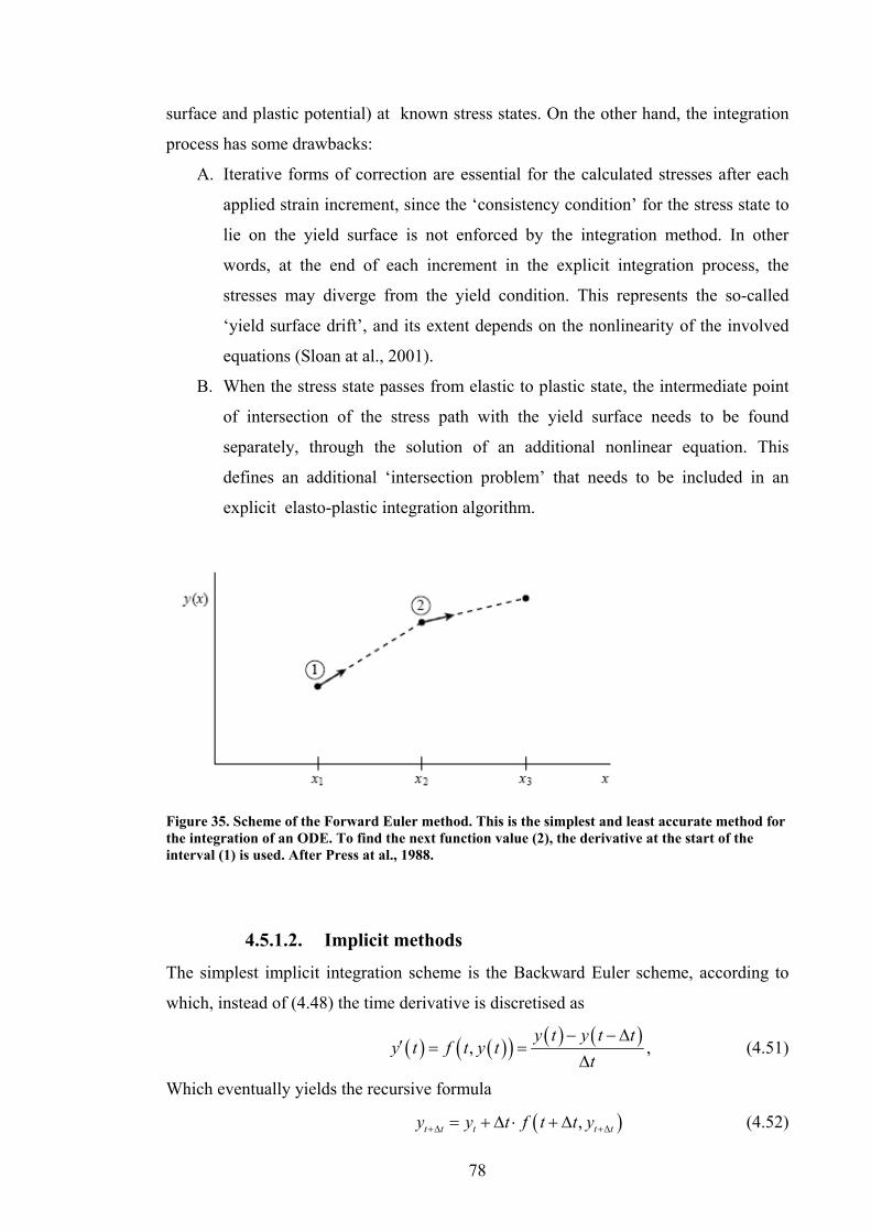
78

surface and plastic potential) at known stress states. On the other hand, the integration

process has some drawbacks:

A. Iterative forms of correction are essential for the calculated stresses after each

applied strain increment, since the ‘consistency condition’ for the stress state to

lie on the yield surface is not enforced by the integration method. In other

words, at the end of each increment in the explicit integration process, the

stresses may diverge from the yield condition. This represents the so-called

‘yield surface drift’, and its extent depends on the nonlinearity of the involved

equations (Sloan at al., 2001).

B. When the stress state passes from elastic to plastic state, the intermediate point

of intersection of the stress path with the yield surface needs to be found

separately, through the solution of an additional nonlinear equation. This

defines an additional ‘intersection problem’ that needs to be included in an

explicit elasto-plastic integration algorithm.

Figure 35. Scheme of the Forward Euler method. This is the simplest and least accurate method for the integration of an ODE. To find the next function value (2), the derivative at the start of the interval (1) is used. After Press at al., 1988.

4.5.1.2. Implicit methods

The simplest implicit integration scheme is the Backward Euler scheme, according to

which, instead of (4.48) the time derivative is discretised as

( ) ( )( ) ( ) ( ),y t y t t

y t f t y tt

− −Δ′ = =

Δ, (4.51)

Which eventually yields the recursive formula

( ),t t t t ty y t f t t y+Δ +Δ= + Δ ⋅ + Δ (4.52)

79

where the function needs to be evaluated at the unknown time-step ( )t t+ Δ . The

dependence of the right-hand side on the variables at ( )t t+ Δ rather than t implies the

inability to solve the equation directly for t ty +Δ .

Implicit methods in plasticity do not require the computation of either the stress

correction (described above, at point A), or the intersection with the yield surface (point

B above), but since the unknown quantities are evaluated at unknown stress states,

integration requires solving iteratively a system of non-linear equations. A well-known

implicit method is the Backward Euler Return scheme, which has been effectively

applied to metal plasticity problems as well as critical state soil mechanics (Borja and

Lee, 1990). Nevertheless, In order to apply an implicit iteration scheme, second

derivatives of the yield function ad plastic potential are required, which is a particularly

difficult and time-consuming task for complex constitutive relations such as those

belonging to the Cam Clay family, especially when thermal effects are included.

Figure 36. Fourth-order Runge-Kutta method. The derivative at point n+1 is calculated from the known value at 1 (filled-in dot) and three trial values at 2,3,4 (open dots). After Press at al., 1988.

4.5.1.3. A refined explicit scheme

We can observe that explicit methods are more suitable to our purpose, since they

require only first derivatives of the involved quantities and are therefore more reliable

and efficient for complex constitutive laws like the ones featuring the thermoplasticity

problem at hand.

A particularly suitable ‘refined explicit’ integration scheme with ‘automatic error

control’ is that proposed by Sloan et al. (2001), which has been shown to be robust and

efficient to integrate constitutive models of the Cam-Clay family. This method is

80

‘refined’ in that the drawbacks of basic explicit schemes are overcome by implementing

additional improvement schemes specifically aimed to the solution of complex soil

elasto-plastic constitutive relationships. Sloan’s scheme is able to deal with non-linear

elasticity, and is easy to generalise since most of the algorithm is independent of the

precise form of the stress-strain relationship.

Key features of this algorithm are:

• Correction of ‘yield surface drift’ (Section 4.5.1.1): stresses are restored to the

yield surface after each integration step, by solving a single nonlinear equation.

• Automatic error control: a local measure of the error in the computed stresses is

estimated with a modified Euler scheme, and used to automatically sub-

increment the imposed strain increment.

• Automatic step-size control (Section 4.5.1.1): The size of each sub-increment

varies throughout the integration process, depending on the non-linearity of the

constitutive relations.

4.5.2. Strain-controlled integration scheme

We hereby propose a general thermoplastic integration scheme for a soil element.

Unlike Laloui et al (2005), we formulate the equations so that we control the strains

(instead of the stresses), to make it easier in the future to generalise the model to 2- and

3-D analyses and to have it ready for a prospective Finite Element implementation.

In order to integrate equations (4.47), it is convenient to define a ‘pseudo-time’ τ:

( )0t t tτ = − Δ (4.53)

where 0t is the time at the start of load increment, 0t t+ Δ the time at the end of load

increment, and [ ]0,1τ ∈ . Applying the chain rule of differentiation to the equations

(4.47) yields

( )mep tep me te te mee

d gd

θ λ θτ= + = Δ −Δ + − Δσ

σ D ε D σ D D C D , (4.54)

cd A Bdσ θ λτ

= ⋅Δ + ⋅Δ , (4.55)

where

( )1 2me tef f fH θλ θ⎡ ⎤Δ = Δ + + Δ⎣ ⎦σ σD ε D . (4.56)

Equations (4.54) and (4.55) can be integrated over the pseudo-time interval [ ]0,1τ ∈ .

81

The known values are the imposed total strain and temperature increments, Δε , θΔ ,

together with the initial values of the stresses (σ0), temperature (θ0), apparent

preconsolidation stress ( 0cσ ′ ) and critical state parameter (M0) at the start of the pseudo-

time increment. The unknown value is the stress increment, to be found once the

increment in preconsolidation pressure (our ‘hardening parameter’) has been computed.

In the following, we will modify Sloan’s (2001) integration scheme to include thermal

effects according to the above presented modified thermo-mechanical constitutive

relations, starting from the above listed initial conditions of our problem.

4.5.3. Elasticity domain and yield surface intersection

Given a vector of externally imposed total strain increment totΔε , a ‘trial’ stress

increment in the elastic domain can be calculated as

me me te θΔ = Δ + Δσ D ε D (4.57) where

me tot teΔ = Δ −Δε ε ε (4.58)

and te te θΔ = Δε C , from Equation (4.16). Nevertheless, since in our case elasticity is

nonlinear, the stress-dependent moduli K and G should be integrated for p′ and vε to

give the secant elastic moduli ( ), vK εΔσ and ( ), vG εΔσ (Sloan, 2001) featuring in the

secant elasticity matrix ( )0 ,me

vεΔD σ , derived from (4.22), where

3

1

totv kk

k

ε ε=

Δ = Δ∑ . (4.59)

In the same way, the secant bulk modulus ( ), vK εΔσ also features in the secant thermo-

elasticity matrix ( )0 ,te

vεΔD σ , derived from (4.23).

By employing the secant elasticity matrices, Equation (4.57) becomes

me teme θΔ = Δ + Δσ D ε D . (4.60)

This stress increment Δσ is used as a check on whether the stress state has changed

from elastic to plastic due to the current strain and temperature increments. If by

applying Δσ the stress state remains within the elastic domain, the new stress state will

be calculated as 0 + Δσ σ , as described in Section 4.5.4 at point (2). If instead the yield

surface is met, it is necessary to calculate the fraction of applied (mechanical and

thermal) strains responsible for the ‘elastic part’ of the stress increment, i.e. the path

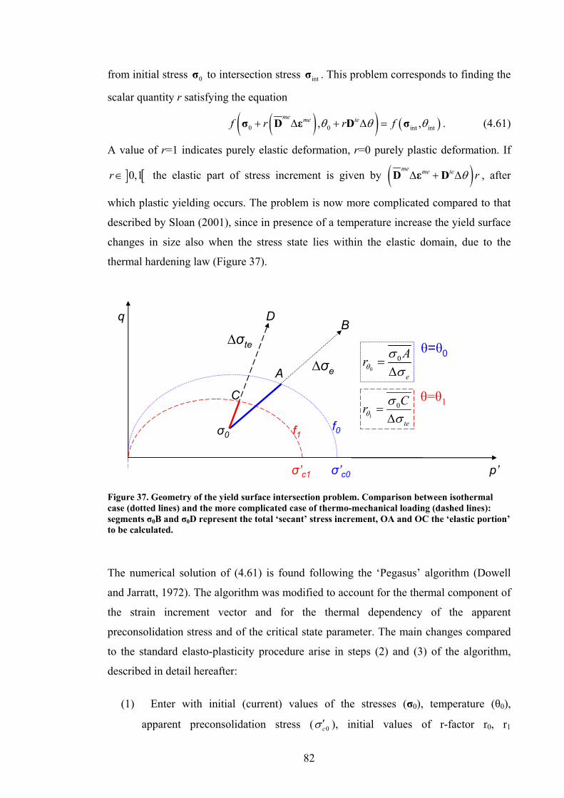
82

from initial stress 0σ to intersection stress intσ . This problem corresponds to finding the

scalar quantity r satisfying the equation

( )( ) ( )0 0 int int, ,me me tef r r fθ θ θ+ Δ + Δ =σ D ε D σ . (4.61)

A value of r=1 indicates purely elastic deformation, r=0 purely plastic deformation. If

] [0,1r∈ the elastic part of stress increment is given by ( )me me te rθΔ + ΔD ε D , after

which plastic yielding occurs. The problem is now more complicated compared to that

described by Sloan (2001), since in presence of a temperature increase the yield surface

changes in size also when the stress state lies within the elastic domain, due to the

thermal hardening law (Figure 37).

σ0

A ∆σe

∆σte

σ’c0σ’c1

f0f1

B

C

D

p’

q

0

0

e

Arθσσ

=Δ

1

0

te

Crθσσ

=Δ

θ=θ0

θ=θ1

Figure 37. Geometry of the yield surface intersection problem. Comparison between isothermal case (dotted lines) and the more complicated case of thermo-mechanical loading (dashed lines): segments σ0B and σ0D represent the total ‘secant’ stress increment, OA and OC the ‘elastic portion’ to be calculated.

The numerical solution of (4.61) is found following the ‘Pegasus’ algorithm (Dowell

and Jarratt, 1972). The algorithm was modified to account for the thermal component of

the strain increment vector and for the thermal dependency of the apparent

preconsolidation stress and of the critical state parameter. The main changes compared

to the standard elasto-plasticity procedure arise in steps (2) and (3) of the algorithm,

described in detail hereafter:

(1) Enter with initial (current) values of the stresses (σ0), temperature (θ0),

apparent preconsolidation stress ( 0cσ ′ ), initial values of r-factor r0, r1

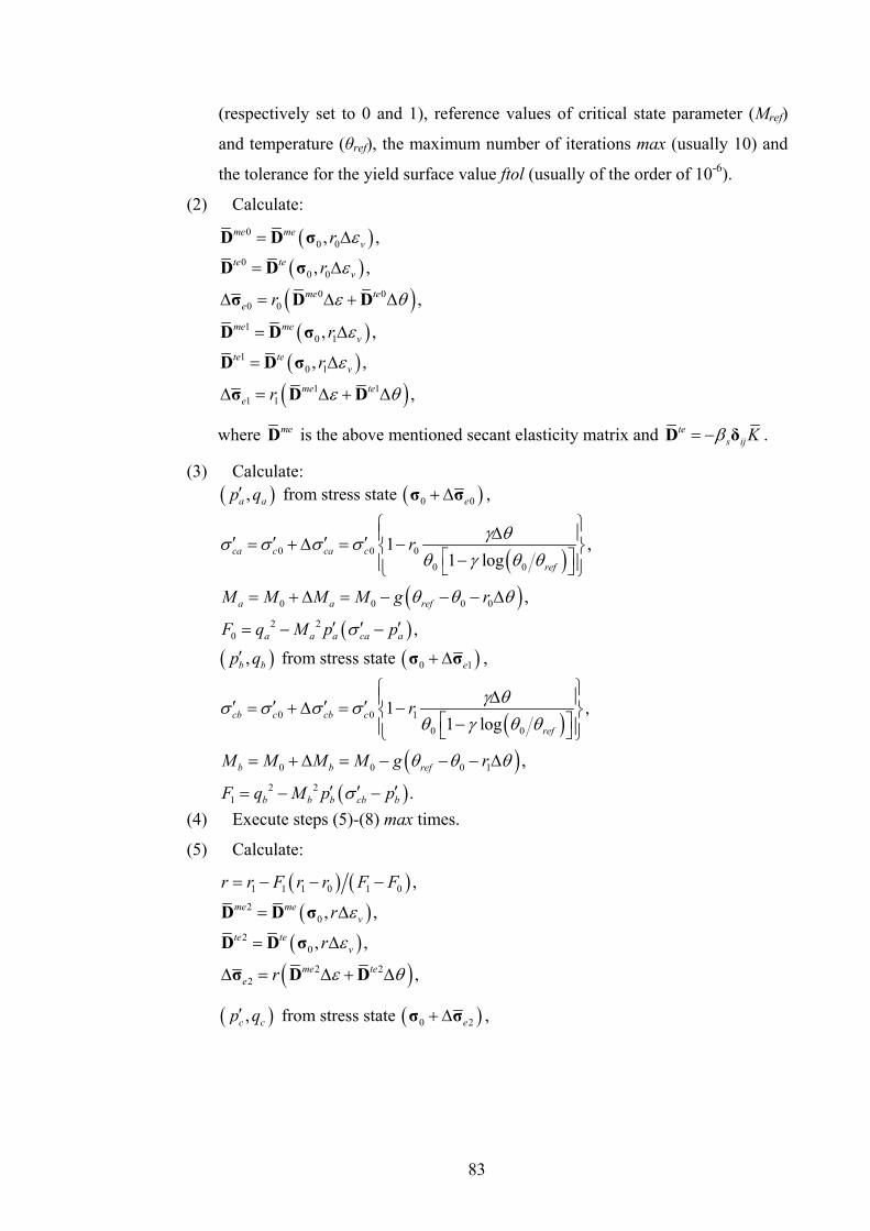
83

(respectively set to 0 and 1), reference values of critical state parameter (Mref)

and temperature (θref), the maximum number of iterations max (usually 10) and

the tolerance for the yield surface value ftol (usually of the order of 10-6).

(2) Calculate:

( )( )( )( )( )( )

00 0

00 0

0 00 0

10 1

10 1

1 11 1

, ,

, ,

,

, ,

, ,

,

me mev

te tev

me tee

me mev

te tev

me tee

r

r

r

r

r

r

ε

ε

ε θ

ε

ε

ε θ

= Δ

= Δ

Δ = Δ + Δ

= Δ

= Δ

Δ = Δ + Δ

D D σ

D D σ

σ D D

D D σ

D D σ

σ D D

where meD is the above mentioned secant elasticity matrix and tes ij Kβ= −D δ .

(3) Calculate: ( ),a ap q′ from stress state ( )0 0e+ Δσ σ ,

( )( )

( )

0 0 00 0

0 0 0 0

2 20

1 ,1 log

,

,

ca c ca cref

a a ref

a a a ca a

r

M M M M g r

F q M p p

γ θσ σ σ σθ γ θ θ

θ θ θ

σ

⎧ ⎫Δ⎪ ⎪′ ′ ′ ′= + Δ = −⎨ ⎬⎡ ⎤−⎪ ⎪⎣ ⎦⎩ ⎭

= + Δ = − − − Δ

′ ′ ′= − −

( ),b bp q′ from stress state ( )0 1e+ Δσ σ ,

( )( )

( )

0 0 10 0

0 0 0 1

2 21

1 ,1 log

,

.

cb c cb cref

b b ref

b b b cb b

r

M M M M g r

F q M p p

γ θσ σ σ σθ γ θ θ

θ θ θ

σ

⎧ ⎫Δ⎪ ⎪′ ′ ′ ′= + Δ = −⎨ ⎬⎡ ⎤−⎪ ⎪⎣ ⎦⎩ ⎭

= + Δ = − − − Δ

′ ′ ′= − −

(4) Execute steps (5)-(8) max times.

(5) Calculate:

( ) ( )( )

( )( )

1 1 1 0 1 0

20

20

2 22

,

, ,

, ,

,

me mev

te tev

me tee

r r F r r F F

r

r

r

ε

ε

ε θ

= − − −

= Δ

= Δ

Δ = Δ + Δ

D D σ

D D σ

σ D D

( ),c cp q′ from stress state ( )0 2e+ Δσ σ ,

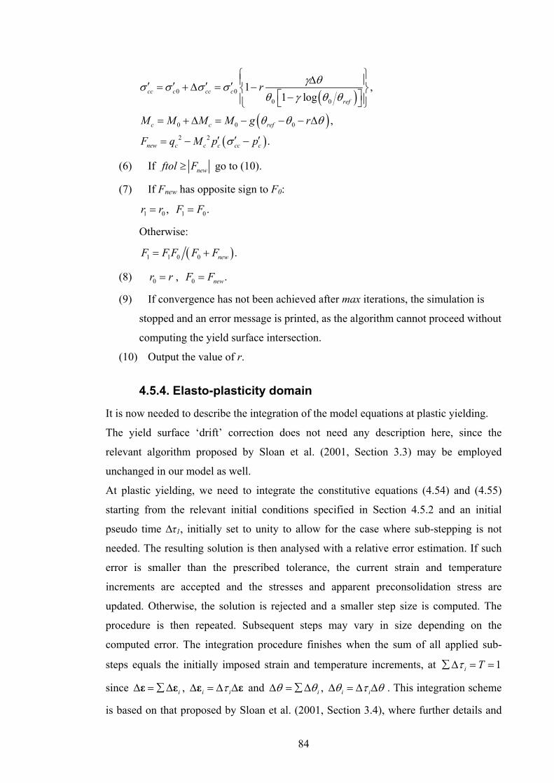
84

( )( )

( )

0 00 0

0 0 0

2 2

1 ,1 log

,

.

cc c cc cref

c c ref

new c c c cc c

r

M M M M g r

F q M p p

γ θσ σ σ σθ γ θ θ

θ θ θ

σ

⎧ ⎫Δ⎪ ⎪′ ′ ′ ′= + Δ = −⎨ ⎬⎡ ⎤−⎪ ⎪⎣ ⎦⎩ ⎭

= + Δ = − − − Δ

′ ′ ′= − −

(6) If newftol F≥ go to (10).

(7) If Fnew has opposite sign to F0:

1 0 1 0, .r r F F= =

Otherwise:

( )1 1 0 0 .newF F F F F= +

(8) 0 0, .newr r F F= =

(9) If convergence has not been achieved after max iterations, the simulation is

stopped and an error message is printed, as the algorithm cannot proceed without

computing the yield surface intersection.

(10) Output the value of r.

4.5.4. Elasto-plasticity domain

It is now needed to describe the integration of the model equations at plastic yielding.

The yield surface ‘drift’ correction does not need any description here, since the

relevant algorithm proposed by Sloan et al. (2001, Section 3.3) may be employed

unchanged in our model as well.

At plastic yielding, we need to integrate the constitutive equations (4.54) and (4.55)

starting from the relevant initial conditions specified in Section 4.5.2 and an initial

pseudo time ∆τ1, initially set to unity to allow for the case where sub-stepping is not

needed. The resulting solution is then analysed with a relative error estimation. If such

error is smaller than the prescribed tolerance, the current strain and temperature

increments are accepted and the stresses and apparent preconsolidation stress are

updated. Otherwise, the solution is rejected and a smaller step size is computed. The

procedure is then repeated. Subsequent steps may vary in size depending on the

computed error. The integration procedure finishes when the sum of all applied sub-

steps equals the initially imposed strain and temperature increments, at 1i Tτ∑Δ = =

since iΔ = ∑Δε ε , i iτΔ = Δ Δε ε and iθ θΔ = ∑Δ , i iθ τ θΔ = Δ Δ . This integration scheme

is based on that proposed by Sloan et al. (2001, Section 3.4), where further details and

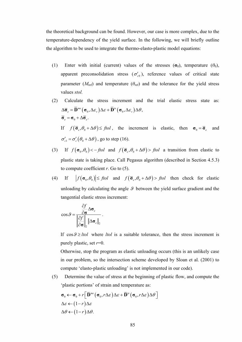
85

the theoretical background can be found. However, our case is more complex, due to the

temperature-dependency of the yield surface. In the following, we will briefly outline

the algorithm to be used to integrate the thermo-elasto-plastic model equations:

(1) Enter with initial (current) values of the stresses (σ0), temperature (θ0),

apparent preconsolidation stress ( 0cσ ′ ), reference values of critical state

parameter (Mref) and temperature (θref) and the tolerance for the yield stress

values stol.

(2) Calculate the stress increment and the trial elastic stress state as:

( ) ( )0 0

0

, , ,.

me tee v v

e e

ε ε ε θΔ = Δ Δ + Δ Δ

= + Δ

σ D σ D σσ σ σ

If ( )0,ef ftolθ θ+ Δ ≤σ , the increment is elastic, then 0 e=σ σ and

( )1 0c cσ σ θ θ′ ′= + Δ , go to step (16).

(3) If ( )0 0,f ftolθ < −σ and ( )0,ef ftolθ θ+ Δ >σ a transition from elastic to

plastic state is taking place. Call Pegasus algorithm (described in Section 4.5.3)

to compute coefficient r. Go to (5).

(4) If ( )0 0,f ftolθ ≤σ and ( )0,ef ftolθ θ+ Δ >σ then check for elastic

unloading by calculating the angle ϑ between the yield surface gradient and the

tangential elastic stress increment:

22

cose

e

f

fϑ

∂Δ

∂=∂

Δ∂

σσ

σσ

.

If cos ltolϑ ≥ where ltol is a suitable tolerance, then the stress increment is

purely plastic, set r=0.

Otherwise, stop the program as elastic unloading occurs (this is an unlikely case

in our problem, so the intersection scheme developed by Sloan et al. (2001) to

compute ‘elasto-plastic unloading’ is not implemented in our code).

(5) Determine the value of stress at the beginning of plastic flow, and compute the

‘plastic portions’ of strain and temperature as:

( ) ( )( )( )

0 0 0 0, ,

1

1 .

me ter r r

r

r

ε ε ε θ

ε ε

θ θ

⎡ ⎤← + Δ Δ + Δ Δ⎣ ⎦Δ ← − Δ

Δ ← − Δ

σ σ D σ D σ

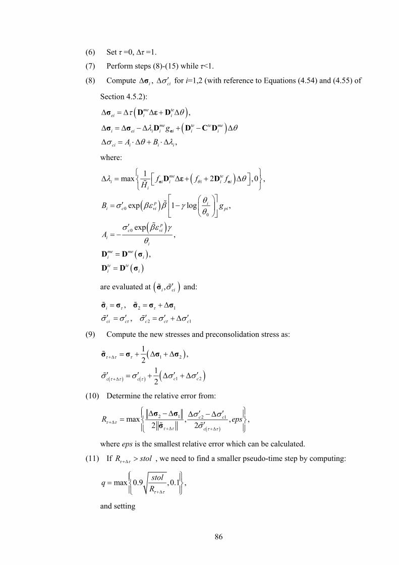
86

(6) Set τ =0, ∆τ =1.

(7) Perform steps (8)-(15) while τ<1.

(8) Compute iΔσ , ciσ ′Δ for i=1,2 (with reference to Equations (4.54) and (4.55) of

Section 4.5.2):

( )( )

,

,

me teei i i

me te te mei ei i i i i i

ci i i i

g

A B

τ θ

λ θ

σ θ λ

Δ = Δ Δ + Δ

Δ = Δ −Δ + − Δ

Δ = ⋅Δ + ⋅Δσ

σ D ε D

σ σ D D C D

where:

( )

( )

( )

( )( )

00

0

1max 2 ,0 ,

exp 1 log ,

exp,

,

me tei i i i i i

i

p ii c vi pi

pc vi

ii

me mei i

te tei i

f f fH

B g

A

θλ θ

θσ βε β γθ

σ βε γ

θ

⎧ ⎫⎡ ⎤Δ = Δ + + Δ⎨ ⎬⎣ ⎦⎩ ⎭⎡ ⎤⎛ ⎞

′= −⎢ ⎥⎜ ⎟⎝ ⎠⎣ ⎦

′= −

=

=

σ σD ε D

D D σ

D D σ

are evaluated at ( ),i ciσ ′σ and:

2 1

2 1

,

, i

ci c c c c

τ τ

τ τσ σ σ σ σ

= = + Δ

′ ′ ′ ′ ′= = + Δ

σ σ σ σ σ

(9) Compute the new stresses and preconsolidation stress as:

( )

( ) ( ) ( )

1 2

1 2

1 ,2

12 c cc c

τ τ τ

τ τ τσ σ σ σ

+Δ

+Δ

= + Δ + Δ

′ ′ ′ ′= + Δ + Δ

σ σ σ σ

(10) Determine the relative error from:

( )

2 1 2 1max , , ,2 2

c c

c

R epsτ ττ τ τ τ

σ σσ+Δ

+Δ +Δ

⎧ ⎫Δ −Δ ′ ′Δ − Δ⎪ ⎪= ⎨ ⎬′⎪ ⎪⎩ ⎭

σ σσ

where eps is the smallest relative error which can be calculated.

(11) If R stolτ τ+Δ > , we need to find a smaller pseudo-time step by computing:

max 0.9 ,0.1 ,stolqRτ τ+Δ

⎧ ⎫⎪ ⎪= ⎨ ⎬⎪ ⎪⎩ ⎭

and setting

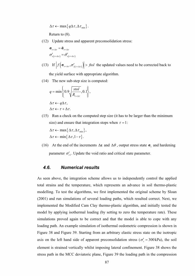
87

{ }minmax ,qτ τ τΔ ← Δ Δ .

Return to (8).

(12) Update stress and apparent preconsolidation stress:

( ) ( )c c

τ τ τ τ

τ τ τ τσ σ+Δ +Δ

+Δ +Δ

=

′ ′=

σ σ

(13) If ( )( ), cf ftolτ τ τ τσ+Δ +Δ′ >σ the updated values need to be corrected back to

the yield surface with appropriate algorithm.

(14) The new sub-step size is computed:

min 0.9 ,0.1 ,stolqRτ τ+Δ

⎧ ⎫⎪ ⎪= ⎨ ⎬⎪ ⎪⎩ ⎭

,.

qτ ττ τ τ

Δ ← ΔΔ ← +Δ

(15) Run a check on the computed step size (it has to be larger than the minimum

size) and ensure that integration stops when 1τ = :

{ }{ }

minmax , ,

min ,1 .

τ τ τ

τ τ τ

Δ ← Δ Δ

Δ ← Δ −

(16) At the end of the increments Δε and θΔ , output stress state 1σ and hardening

parameter 1cσ ′ . Update the void ratio and critical state parameter.

4.6. Numerical results

As seen above, the integration scheme allows us to independently control the applied

total strains and the temperature, which represents an advance in soil thermo-plastic

modelling. To test the algorithms, we first implemented the original scheme by Sloan

(2001) and run simulations of several loading paths, which resulted correct. Next, we

implemented the Modified Cam Clay thermo-plastic algorithm, and initially tested the

model by applying isothermal loading (by setting to zero the temperature rate). These

simulations proved again to be correct and that the model is able to cope with any

loading path. An example simulation of isothermal oedometric compression is shown in

Figure 38 and Figure 39. Starting from an arbitrary elastic stress state on the isotropic

axis on the left hand side of apparent preconsolidation stress ( 300cσ ′ = kPa), the soil

element is strained vertically whilst imposing lateral confinement. Figure 38 shows the

stress path in the MCC deviatoric plane, Figure 39 the loading path in the compression

88

plane. It can be noticed in Figure 38 that the loading path approaches the yield surface,

follows it towards the right for a while, to finally start to exhibit (at about p’=250 kPa,

or Ln(p’)=5.5) plastic hardening (thus determining the enlargement of the yield locus)

which is then indefinitely continued along a constant load path, without reaching the

critical state. We remark that the initial part of the stress path in Figure 38 is not

representative of a standard oedometer test, due to the initial conditions of our

simulation: to reproduce over-consolidation, an isotropic apparent preconsolidation

stress (consistently with the MCC framework) has been imposed as initial condition for

an oedometric loading simulation. Had we also simulated the sample preparation by 1-D

consolidation and subsequent elastic swelling, the loading path would have started at a

higher p’ in the isotropic axis, resulting in a smoother transition between the elastic and

plastic states.

Finally, we tested the full potential of our thermo-elasto-plastic integration algorithm.

The response of a soil element to different strain and temperature paths is demonstrated

in Figure 40. For these example simulations, the following parameter values were

chosen: 0.3ν = , 0.02κ = , 0.2λ = , OCR=5, 0.3γ = , 36 10g −= ⋅ . The initial

temperature, critical state parameter and void ratio were set respectively to 20refθ = °C,

=0.8refM , 0.7refe = . The dashed line represents isothermal loading while the solid line

represents thermo-mechanical loading, experiencing the same total straining as the

isothermal case superimposed with a 40°C total temperature increase. The dash-dotted

path was obtained by applying a higher temperature rate at the beginning (40°C of total

increase concentrated during the first 1/20 of overall straining), followed by mechanical

loading only. It is shown how the apparent preconsolidation stress decreases as

temperature increases, and how the slope of the plastic loading path changes if

temperature and mechanical strains are applied at the same time.

In Figure 41 numerical results are compared to some experimental data on three

isothermal isotropic compression paths carried out at different temperatures (Laloui &

Cekerevac, 2003). In accordance with the experimental data, for these simulations

22refθ = °C, 0.075κ = and 0.11λ = . The red line simulates an isothermal loading path

at ambient temperature. The black line represents a combined thermo-mechanical

loading path to simulate the transition between two isothermal loading data sets, where

temperature is increased from 22°C to 60°C alongside mechanical straining (path 0 to 2)

while experiencing the same void ratio change as that obtained in Laloui and

89

Cekerevac’s (2003) isobaric heating tests (path 0 to 1). After point 2, mechanical

loading only follows. Good agreement with experimental data points is achieved in both

cases.

0

50

100

150

200

250

0 100 200 300 400 500 600 700 800 900 1000 1100

p' (kPa)

q (k

Pa) Stress path

Initial yield surface

odometric path – deviatoric plane

00 100 200 300 400 500 600 700 800 900 1000 1100

p' (kPa)

subsequent yield surface

q (k

Pa)

p’ (kPa)

Figure 38. Numerical simulations with our code of isothermal oedometric compression of a soil element. Loading path in deviatoric plane (p’, q)

0.35

0.4

0.45

0.5

0.55

0.6

0.65

0.7

0.75

3 3.5 4 4.5 5 5.5 6 6.5 7

ln p'

void

rat

io

odometric path – compression plane

Figure 39. Numerical simulations with our code of isothermal oedometric compression of a soil element. Loading path in compression plane (ln(p’), e).

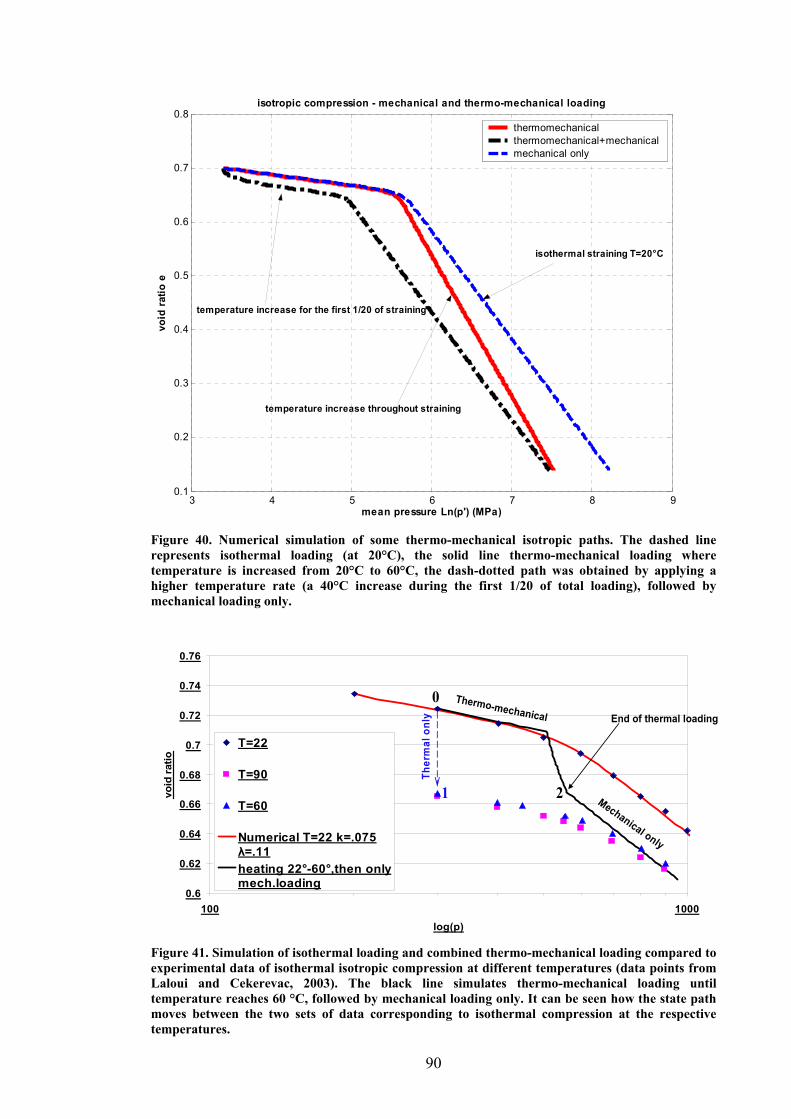
90

3 4 5 6 7 8 90.1

0.2

0.3

0.4

0.5

0.6

0.7

0.8

mean pressure Ln(p') (MPa)

void

rat

io e

isotropic compression - mechanical and thermo-mechanical loading

thermomechanicalthermomechanical+mechanicalmechanical only

temperature increase for the first 1/20 of straining

temperature increase throughout straining

isothermal straining T=20°C

Figure 40. Numerical simulation of some thermo-mechanical isotropic paths. The dashed line represents isothermal loading (at 20°C), the solid line thermo-mechanical loading where temperature is increased from 20°C to 60°C, the dash-dotted path was obtained by applying a higher temperature rate (a 40°C increase during the first 1/20 of total loading), followed by mechanical loading only.

0.6

0.62

0.64

0.66

0.68

0.7

0.72

0.74

0.76

100 1000log(p)

void

ratio

T=22

T=90

T=60

Numerical T=22 k=.075λ=.11heating 22°-60°,then onlymech.loading

Ther

mal

onl

y

Thermo-mechanical End of thermal loading

1

0

Mechanical only

2

Figure 41. Simulation of isothermal loading and combined thermo-mechanical loading compared to experimental data of isothermal isotropic compression at different temperatures (data points from Laloui and Cekerevac, 2003). The black line simulates thermo-mechanical loading until temperature reaches 60 °C, followed by mechanical loading only. It can be seen how the state path moves between the two sets of data corresponding to isothermal compression at the respective temperatures.

91

Chapter 5. Modified landslide model

The system of governing equations for Vardoulakis’ landslide model seen in Section

2.3.4 provides a 1-D analysis of the phenomenon, employing a simple Mohr-Coulomb

yield locus as soil constitutive model. To provide a more realistic constitutive

assumption, which can be more easily generalised for applications to a wider range of

soils, we will now modify the landslide model governing equations to include the

thermoplastic model described in Chapter 4. The three equations forming system (2.6)

will be studied one by one, and changed to take into account the new constitutive law.

After modification, the model will be ready for numerical implementation, and can be

validated through the back-analysis of a catastrophic landslide case history. The large

amount of information on the geological and geomechanical aspects of Vajont (cf.

Section 2.1.4) makes it the ideal case study to back-analyse for this purpose.

5.1. Model assumptions and overview

The two main constitutive assumptions of the modified landslide model which are

essential before a systematic description of the equations are those of plane strain and of

critical state for the soil inside the shearband. Both are consistent with Vardoulakis

(2000, 2002a).

According to the continuum mechanics definition, a state of plane strain exists at a point

when one and only one of the principal strains is zero (Mase, 1970). In an elasto-plastic

problem, plane strain implies in-plane deformation, i.e. the deformation field is identical

in all planes perpendicular to the direction of the zero principal strain. With reference to

Figure 42, in the shearband problem the direction of zero principal strain is the out-of-

plane one, i.e. along axis y, while the x axis points in the direction of movement, and the

z axis is taken perpendicular to it. Therefore, in plane strain the following conditions

hold:

0

0

0

yy

zy yz

xy yx

ε

γ γ

γ γ

=

= =

= =

(5.1)

and the strain tensor is simplified to

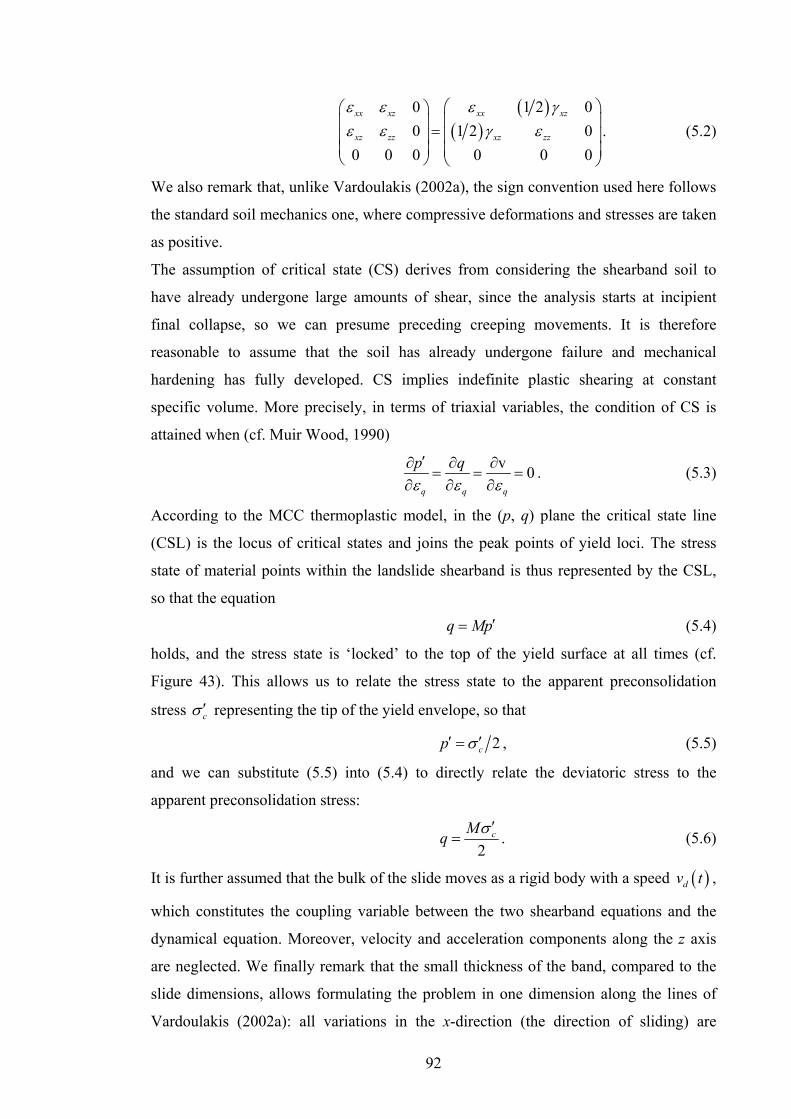
92

( )

( )0 1 2 00 1 2 0

0 0 0 0 0 0

xx xz xx xz

xz zz xz zz

ε ε ε γε ε γ ε

⎛ ⎞⎛ ⎞⎜ ⎟⎜ ⎟ = ⎜ ⎟⎜ ⎟

⎜ ⎟ ⎜ ⎟⎝ ⎠ ⎝ ⎠

. (5.2)

We also remark that, unlike Vardoulakis (2002a), the sign convention used here follows

the standard soil mechanics one, where compressive deformations and stresses are taken

as positive.

The assumption of critical state (CS) derives from considering the shearband soil to

have already undergone large amounts of shear, since the analysis starts at incipient

final collapse, so we can presume preceding creeping movements. It is therefore

reasonable to assume that the soil has already undergone failure and mechanical

hardening has fully developed. CS implies indefinite plastic shearing at constant

specific volume. More precisely, in terms of triaxial variables, the condition of CS is

attained when (cf. Muir Wood, 1990)

v 0q q q

p qε ε ε′∂ ∂ ∂= = =

∂ ∂ ∂. (5.3)

According to the MCC thermoplastic model, in the (p, q) plane the critical state line

(CSL) is the locus of critical states and joins the peak points of yield loci. The stress

state of material points within the landslide shearband is thus represented by the CSL,

so that the equation

q Mp′= (5.4)

holds, and the stress state is ‘locked’ to the top of the yield surface at all times (cf.

Figure 43). This allows us to relate the stress state to the apparent preconsolidation

stress cσ ′ representing the tip of the yield envelope, so that

2cp σ′ ′= , (5.5)

and we can substitute (5.5) into (5.4) to directly relate the deviatoric stress to the

apparent preconsolidation stress:

2

cMq σ ′= . (5.6)

It is further assumed that the bulk of the slide moves as a rigid body with a speed ( )dv t ,

which constitutes the coupling variable between the two shearband equations and the

dynamical equation. Moreover, velocity and acceleration components along the z axis

are neglected. We finally remark that the small thickness of the band, compared to the

slide dimensions, allows formulating the problem in one dimension along the lines of

Vardoulakis (2002a): all variations in the x-direction (the direction of sliding) are

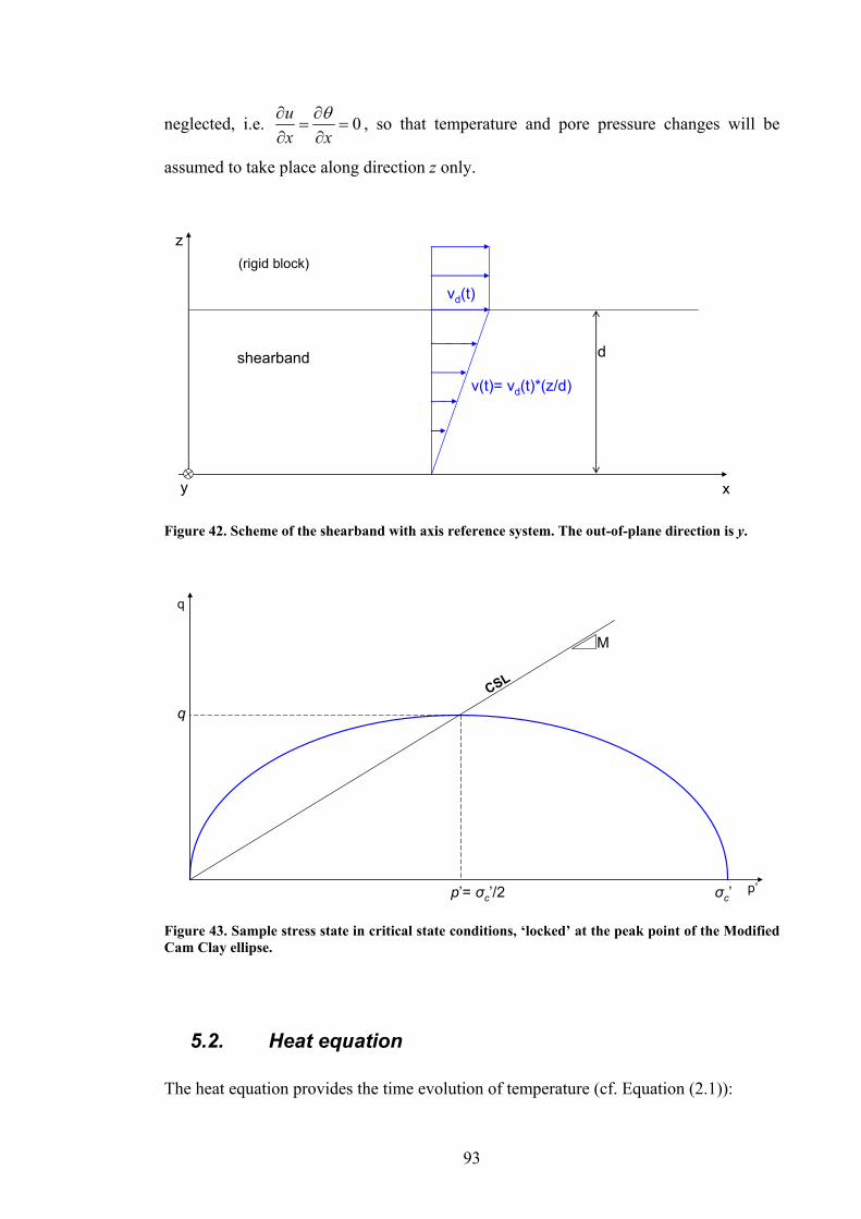
93

neglected, i.e. 0ux x

θ∂ ∂= =

∂ ∂, so that temperature and pore pressure changes will be

assumed to take place along direction z only.

y x

z

d

vd(t)

v(t)= vd(t)*(z/d)

shearband

(rigid block)

Figure 42. Scheme of the shearband with axis reference system. The out-of-plane direction is y.

p’

q

σc

CSL

M

σc’p’= σc’/2

q

Figure 43. Sample stress state in critical state conditions, ‘locked’ at the peak point of the Modified Cam Clay ellipse.

5.2. Heat equation

The heat equation provides the time evolution of temperature (cf. Equation (2.1)):

94

2

2mf

Dkt z Cθ θ∂ ∂= +

∂ ∂ (5.7)

In the following, the modifications to (5.7) necessary to accommodate the new

constitutive model of Chapter 4 are detailed.

The dissipation term, corresponding to the plastic work within the shearband, accounts

for all heat generation, and is expressed as

pD τγ≈ (5.8)

where the shear stress is τ μσ ′= , due to the assumed Mohr-Coulomb constitutive law,

and the plastic shear deformation p vz

γ ∂=∂

. All dissipation within the fluid is neglected.

To employ the CS thermoplastic soil model, dissipation needs to be expressed in a

generalised form.

Dissipation can be reformulated in the principal stress space as:

1 1 2 2 3 3p p pD σ ε σ ε σ ε= + + . (5.9)

Substituting the plastic strain rate components with the flow rule relationship (4.10)

yields

1 2 31 2 3

f f fD λ σ σ σσ σ σ

⎡ ⎤∂ ∂ ∂= + +⎢ ⎥∂ ∂ ∂⎣ ⎦

(5.10)

where 1σ , 2σ and 3σ are the principal stresses, f is the yield locus (used also as a

plastic potential) and λ is the plastic multiplier.

Expression (5.10) now needs to be specified in terms of the constitutive relationship. In

principal stress space, the Modified Cam Clay yield surface f can be written in the

general case of 1 2 3σ σ σ′ ′ ′≠ ≠ in terms of the three stress invariants, i.e. the mean

principal effective stress p’, the stress deviator J and the Lode angle θL (e.g. see Potts

and Zdravkovic, 1999):

( )2 2J cf J M p pσ′ ′ ′= − − (5.11)

where:

( )1 2 313

p σ σ σ′ ′ ′ ′= + + (5.12)

( ) ( ) ( )2 2 22 3 3 1 1 2

16 3

qJ σ σ σ σ σ σ′ ′ ′ ′ ′ ′= − + − + − = (5.13)

2 3

1 3

1arctan 2 13L

σ σθσ σ

⎡ ⎤⎛ ⎞′ ′−= −⎢ ⎥⎜ ⎟′ ′−⎝ ⎠⎣ ⎦

. (5.14)

95

In the above, MJ is a generalised critical state parameter depending on the Lode angle

and the critical state angle of shearing resistance csϕ′ :

sinsin sincos

3

csJ

L csL

M ϕθ ϕθ

′= ′

+ (5.15)

In plane strain conditions, it is normally assumed θL=0, so that (5.15) becomes

sinJ csM ϕ′= . (5.16)

The classic expression for the MCC yield surface adopted in Chapter 4 is

( )2 2cf q M p pσ′ ′ ′= − − , (5.17)

where, consistently with (5.13),

( ) ( ) ( )2 2 22 3 3 1 1 2

12

q σ σ σ σ σ σ⎡ ⎤′ ′ ′ ′ ′ ′= − + − + −⎣ ⎦ . (5.18)

As a consequence, expression (5.17) in terms of ( ),p q′ is equivalent to (5.11) only if

3 sin 3J csM M ϕ′= = . (5.19)

We shall therefore adopt for the yield locus the form (5.17) together with expression

(5.19) for the CS parameter throughout the analysis. The derivative of the yield surface

with respect to the principal stress components can be expressed as a function of the

invariants p and q as

i i i

f f p f qp qσ σ σ

′∂ ∂ ∂ ∂ ∂= +

′∂ ∂ ∂ ∂ ∂. (5.20)

From the definitions (5.12), (5.17) and (5.18) we can calculate the above derivatives as:

( )2 2 cf M pp

σ∂ ′ ′= −′∂

, (5.21)

13i

pσ′∂=

∂, (5.22)

2f qq∂

=∂

, (5.23)

( )32i

i

pqq

σσ

′−∂=

∂. (5.24)

Recalling that the soil is at critical state, substituting (5.5) into Equation (5.21) yields

0fp∂

=′∂

. (5.25)

By using equations (5.22)-(5.25) into (5.20) we get the equations (for i=1,2,3)

( )3 ii

f pσσ∂ ′= −∂

, (5.26)

96

which can be substituted into (5.10) to obtain, by employing the definition of mean

effective stress (5.12):

( ) ( ) ( )

( )( ) ( ) ( )

1 1 2 2 3 3

2 2 21 2 3 1 2 1 3 2 3

2 2 21 2 3 1 2 3

3 3 3

2

.

D p p pλ σ σ σ σ σ σ

λ σ σ σ σ σ σ σ σ σ

λ σ σ σ σ σ σ

′ ′ ′= − + − + − =⎡ ⎤⎣ ⎦⎡ ⎤= + + − − − =⎣ ⎦⎡ ⎤= − + − + −⎣ ⎦

(5.27)

Recalling the definition of deviatoric stress (5.18), (5.27) becomes

22D qλ= , (5.28)

which by substituting the CS condition (5.6) finally yields

( )2

2122 2

cc

MD Mσλ λ σ′⎛ ⎞ ′= =⎜ ⎟

⎝ ⎠. (5.29)

Equation (5.29) represents the dissipation term at CS for plane strain, in general stress

space. It is now needed to specify the terms M, cσ ′ and λ in relation to the

thermoplastic CS model of Chapter 4. This is done in the following subsections, 5.2.1 to

5.2.3.

5.2.1. Material softening law

In CS soil mechanics, parameter M is constant, and in our case corresponds to the soil

(measured) friction angle, sin 3M ϕ′= according to (5.19). On the other hand,

prolonged and fast shearing along a defined failure plane often brings about a drop in

the friction angle of clays, due to the aligning of the platy particles parallel to the

direction of shearing, until the ‘residual state’ is reached. We may now adjust our CS

framework in order to approximate such residual state behaviour, under constant

volume conditions, by accounting for the reduction of friction angle ϕ′ with

displacement and velocity. This can be done following the strain- and strain-rate

softening law proposed by Vardoulakis (2002a). Furthermore, according to the adopted

thermoplastic model we may allow within the CS framework for possible thermal-

friction softening behaviour, as observed in some soils and already discussed in

Sections 3.4.3.3 and 4.4.1.

Regarding strain- and strain-rate friction softening (Section 2.3.4), we shall start from

the simple laws defined by Vardoulakis (2002a) for the Vajont clay based on the ring

shear experimental data of Tika and Hutchinson (1999). Such laws define the evolution

of the friction coefficient μ̂ , related to the soil mobilised friction angle as ˆ tanμ φ′= , as

a hyperbolic function:

97

( )1

1ˆ1

r p rdxa

d

μ μ μ μ= + −+

(5.30)

where

( )2

1

1r rd rs rd

dvad

μ μ μ μ= + −+

. (5.31)

In the above d is the shearband thickness, xd the slide displacement and vd the slide

velocity, so that the (thickness-dependent) shear strain is dxd

γ ≈ and its rate dvd

γ ≈ .

The limiting values rsμ and rdμ are respectively the static and dynamical residual

friction coefficients, while pμ is the initial value of friction coefficient and

1 20.114, 0.103a a= = are numerical factors defining how quickly the static and

dynamic coefficients respectively decrease with displacement and velocity. The

material-friction softening critical state parameter M̂ can be written using (5.30): since

( )ˆarctanϕ μ′ = and sin 3M ϕ′= , we obtain

( )ˆ ˆ3 sin arctanM μ= ⎡ ⎤⎣ ⎦ . (5.32)

An alternative form of (5.32), which could be more convenient for algebraic

manipulation, can be found through the trigonometric identity (e.g. see Abramowitz and

Stegun, 1964)

( )2

arctan arcsin1

yyy

⎛ ⎞⎜ ⎟=⎜ ⎟+⎝ ⎠

(5.33)

which allows us to express (5.32) as

2

ˆˆ 3ˆ1

M μμ

=−

. (5.34)

Furthermore, we will allow for an additional mechanism of thermal-friction softening,

by employing the linear law (4.2). The final expression for the critical state parameter is

the result of superposition of the frictional displacement- ,velocity- and thermal-

softening effects, so that parameter M starts from a reference value and decreases

towards zero according to the following expression:

( ) ( )ˆ( , , ) , refM M gγ γ θ γ γ θ θ= − − (5.35)

98

where refθ is the reference temperature and parameter g is the rate of decrease of M

with temperature, or ‘thermal sensitivity’, which can be calibrated on experimental data

such as those reported in Figure 30.

It must be here observed that the thermal-friction softening mechanism, being linear, is

not bounded from below and may lead to unrealistic negative, or excessively small,

values for the friction coefficient. On the other hand, a linear decrease law is the

simplest and most effective one available to interpret the scarce experimental data

available. We therefore choose to adopt it and impose an arbitrary lower limit for M,

rather than adopt a more complex law such as the exponential one proposed by

Vardoulakis (2002b). In the absence of direct experimental evidence, the lower-bound

value ML is set equal to the dynamic residual value, ( )3 sin arctanL rdM μ= ⎡ ⎤⎣ ⎦ .

5.2.2. Thermal hardening law defining the stress state

The apparent preconsolidation stress cσ ′ , defining the size of the yield envelope,

evolves with temperature and volumetric plastic strain according to the thermo-

mechanical hardening law (4.1). However, at critical state its dependency is reduced to

the thermal component only, since the plastic volumetric strain rate is zero.

We now need to allow for the presence of excess pore pressures within the shearband.

This means adding a pore-pressure dependency to the hardening relationship, which had

not been considered in Laloui’s thermal model (Section 2.3) as that was derived in a

context of fully drained loading. According to the effective stress principle, the mean

effective stress can be written as

0p p u′ ′= − (5.36)

where 0 Hp p u′ = − is the initial effective mean stress in the shearband before the

occurrence of excess pore pressures, Hu being the equilibrium pore pressure. In critical

state conditions, cσ ′ uniquely defines the stress state since the latter is locked at the top

of the yield envelope, at point ( / 2, / 2)c cMσ σ′ ′ in the ( ),p q plane (Section 5.1). We

can therefore rewrite (5.36), in view of (5.5), as

( ) ( ), 2c cHu uσ θ σ θ′ ′= − , (5.37)

where according to (4.1),

( ) ( )0 exp( ) 1 logpcH c v refσ θ σ βε γ θ θ′ ⎡ ⎤′= −⎣ ⎦ . (5.38)

99

From the above we understand that CS conditions allow us to equivalently consider as

the stress variable either the preconsolidation stress or the mean stress. If one wants to

refer, as is more conventional, to the mean stress p’, the stress state during thermo-poro-

mechanical loading can be expressed as

( ) ( ),p u p uθ θ′ ′= − (5.39)

where ( ) ( ) 2cHp θ σ θ′ ′= according to (5.5).

A demonstration of the above constitutive assumptions is given in Figure 44, which

shows a typical (effective) stress path of a material point within the shearband during

catastrophic sliding. For clarity the contributions of the different mechanisms affecting

the stress state are drawn separately, although they occur at the same time. In a generic

time interval Δt during sliding, the stress state, locked at the top of the yield locus,

follows the path 1-4. From state 1 to 2, thermal softening occurs as the locus shrinks

due to a temperature increase, according to the hardening law (5.38). Path 2 to 3 is due

to the occurrence of excess pore pressures, which reduces by uΔ the effective mean

stress (or equivalently, the apparent preconsolidation stress by 2 uΔ ). Finally, from 3 to

4 frictional softening occurs, causing a decrease in the slope of the CSL and a

consequent further change in stress.

q

σc1

12

3

4

σc2

θ= θ1θ= θ2

Δσc(Δθ)2Δu

σc3σc4

Δσc(ΔM)

CSL 1-3

CSL 4

M=M1

M=M2

p’

Figure 44. Effective stress paths of material points inside the shearband.

100

5.2.3. Plastic multiplier

The plastic multiplier in general stress space λ was calculated in Section 4.4.1 from the

consistency condition, as

( )

2

2

pv

me te

mep

f f ff f f

θ

ε

θλ

′

+ +=

−σ σ

σ

D ε DD

. (5.40)

It is now convenient to express (5.40) in terms of stress invariants, for homogeneity of

notation with the rest of the landslide model equations. No loss in generality occurs,

since it is always possible, for isotropic materials, to split the stress tensor into a

spherical and a deviatoric part (Mase, 1970). The terms featuring in (5.40) can be

rewritten as:

3mep v q qf Kf Gfε ε= +σD ε (5.41)

2 2tes pf K fβ= −σD (5.42)

2 2 23mep qf Kf Gf= +σ D (5.43)

where the partial derivatives of the yield function, from Section 4.4.1 are:

( ){ }( )

( ){ }

2

0

20

20

2 1 log

1 log

2 1 log

2

pv

mm

m

p p m

q

p Mf gp M p

f p M

f g M p

f q

θ

ε

σ λ σ γ θ θθ

σ β γ θ θ

σ γ θ θ′ ′

′ ′′ ′ ′= + − −⎡ ⎤⎣ ⎦

′ ′= − −⎡ ⎤⎣ ⎦

′ ′= = − −⎡ ⎤⎣ ⎦=

(5.44)

In CS conditions, the first term on the RHS of (5.41) is zero since 0vε = , so that the

multiplier (5.40) becomes

0 1qF Fλ ε θ= + (5.45)

where

0

1

3

2

q q

s p

GfF

Hf K f

FH

θ

ε

β

=

−=

(5.46)

and

2 23 pv

p q pH Kf Gf f fε ′= + − . (5.47)

The final step towards the incorporation of (5.45) into the landslide model is expressing

the strain rate qε in terms of the variables of the 1-D shearband problem. A general

form for the distortional (or deviatoric) strain rate is (e.g. see Muir Wood, 1990)

101

( ) ( ) ( ) ( )2 22 2 2 21 2 33q yy zz zz xx xx yy xy yz xzε ε ε ε ε ε ε γ γ γ⎡ ⎤= − + − + − + + +⎢ ⎥⎣ ⎦

. (5.48)

In this case, due to plane strain conditions 0yyε = and 0zy xyγ γ= = . Moreover, 1-D

hypotheses (Figure 42) imply that 0xxε = , and since we are at critical state

0v xx yy zzε ε ε ε= + + = , so that also 0zzε = . Equation (5.48) is therefore reduced to

33q zxε γ= (5.49)

where xzx

vz

γ ∂=∂

, and ( ),xv v z t= is the velocity within the shearband in the direction of

motion, which can be written, using the same assumptions discussed in Section 2.3.4.1,

as

( ) ( ), dzv z t v td

= (5.50)

so that (5.49) becomes

( )3 33 3

dxq

v tvz d

ε ∂= =

∂. (5.51)

Substituting (5.51) into (5.45) yields the final expression for the thermo-plastic

multiplier:

1 2xvF F

t zθλ ∂∂

= +∂ ∂

. (5.52)

Coefficients F1 and 2 03

3F F= depend on the current temperature θ and pore pressure u

through equations (5.46).

5.2.4. Final form of heat equation

All terms featuring in the dissipation term are now fully specified. The heat Equation

(5.7), by adopting expression (5.29) for the dissipation, can then be written as

( )22

2 2c

mf

Mk

t z Cλ σθ θ ′∂ ∂

= +∂ ∂

(5.53)

or, by substituting (5.52),

( )22

1 22 2c x

mf

M vk F Ft z C t z

σθ θ θ′ ∂∂ ∂ ∂⎛ ⎞= + +⎜ ⎟∂ ∂ ∂ ∂⎝ ⎠. (5.54)

By collecting the terms multiplying the temperature rate we obtain

102

( ) ( )2 222

1 212 2

c c xm

f f

M M F vF kt C z C z

σ σθ θ⎛ ⎞′ ′ ∂∂ ∂− = +⎜ ⎟

⎜ ⎟∂ ∂ ∂⎝ ⎠ (5.55)

hence,

( )

( )( )

222

2 221

1

21

2

cm x

c f c

f

M Fk vt z zM C M F

FC

σθ θσ σ

′ ∂∂ ∂= +

∂ ∂ ∂′ ′−−

(5.56)

which, in view of (5.50), can be written as

( )2

2d

i i

v tD F

t z dθ θ∂ ∂= +

∂ ∂ (5.57)

where

( )2

112

mi

c

f

kDM

FCσ

=′

−

, (5.58)

( )( )

222

12c

if c

M FF

C M Fσ

σ

′=

′−. (5.59)

Coefficients iD and iF depend on pore pressure u, temperature θ and, if the material

softening law (5.35) is taken into account, also on the shear strain γ and strain rate γ .

The final form for the heat diffusion-generation equation within the framework of

thermal CS soil mechanics is given by (5.57). Compared to the original equation, (5.7),

it can be noticed that the diffusion term is now non-linear: despite the original thermal

diffusivity km being constant, it is divided by the temperature-dependent factor

( )2

112

c

f

MF

Cσ⎛ ⎞′

−⎜ ⎟⎜ ⎟⎝ ⎠

. Hence, defining the term iD as a new thermal diffusivity allows us to

formally define (5.57) a non-linear diffusion-generation equation.

5.3. Pore pressure equation

The pore pressure equation describes the time evolution of excess pore pressures within

the shearband and its surroundings (cf. Section 2.3.4.1):

v mu uct z z t

θλ∂ ∂ ∂ ∂⎛ ⎞= +⎜ ⎟∂ ∂ ∂ ∂⎝ ⎠. (5.60)

the structure of the consolidation coefficient vc and the pressurisation coefficient mλ

will be now discussed in light of the proposed modifications to the constitutive

framework.

103

5.3.1. Consolidation coefficient

The consolidation coefficient vc is a function of soil compressibility and soil

permeability. It can be expressed as

wv

w

kcg cρ

= , (5.61)

where c is the soil compressibility, g the acceleration of gravity, wρ the pore-fluid

density and wk is Darcy’s permeability coefficient, which is an increasing function of

porosity and fluid density and inversely proportional to the dynamic viscosity of the

fluid (see e.g. Powrie, 1997). Experimental results in Boom clay (Delage et al., 2000)

showed that vc for a clay is expected to be a weakly increasing function of temperature

(Figure 45). Such small variation is due to two opposing effects: the soil permeability

(in the sense of Darcy) increases with temperature, as a consequence of the thermal

decrease of viscosity of the pore fluid, but this effect is compensated by a concurrent

decrease of porosity.

Delage et al. (2000) suggest that the aforementioned thermal variation of vc can be

neglected, in line with other authors who investigated the thermal volumetric behaviour

of clays (e.g., Habibagahi, 1977 and Towhata et al., 1995). Vardoulakis (2002a) on the

other hand, to interpolate the experimental data of Delage et al. (2000) reported in

Figure 45, proposes the exponential function

( )0 expv v cc c θ θ= (5.62)

where 8 20 6.346 10 m / svc −= × and 389.15 Ccθ = ° . These experimental results

according to Vardoulakis (2002a) are not representative of a deforming shearband

undergoing pressurisation, and need to be adjusted to the considered ‘elastic unloading’

stress path in the landslide model, so cv is recalculated as a function of the permeability

and compressibility of the soil (Section 5.3.2.3) through Equation (5.61). This yields a

still weakly increase of cv with temperature, but at higher values (Figure 46) compared

to Delage et al.’s (2000) results, given the relatively small value obtained for

compressibility. Based on these data, Vardoulakis suggests a mean value for the

consolidation coefficient of water-saturated clay:

8 27.3 10 m svc −= × . (5.63)

The above considerations suggest that the variation of consolidation coefficient with

temperature is not significant in our context. In fact, the thermal change of cv at thermo-

plastic states is less than an order of magnitude (Figure 45). This is also consistent with

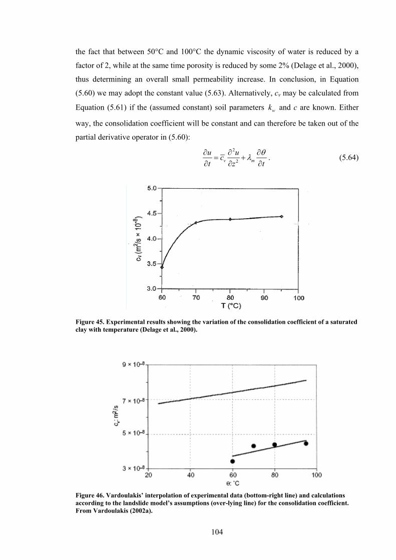
104

the fact that between 50°C and 100°C the dynamic viscosity of water is reduced by a

factor of 2, while at the same time porosity is reduced by some 2% (Delage et al., 2000),

thus determining an overall small permeability increase. In conclusion, in Equation

(5.60) we may adopt the constant value (5.63). Alternatively, cv may be calculated from

Equation (5.61) if the (assumed constant) soil parameters wk and c are known. Either

way, the consolidation coefficient will be constant and can therefore be taken out of the

partial derivative operator in (5.60):

2

2v mu uct z t

θλ∂ ∂ ∂= +

∂ ∂ ∂. (5.64)

Figure 45. Experimental results showing the variation of the consolidation coefficient of a saturated clay with temperature (Delage et al., 2000).

Figure 46. Vardoulakis’ interpolation of experimental data (bottom-right line) and calculations according to the landslide model’s assumptions (over-lying line) for the consolidation coefficient. From Vardoulakis (2002a).

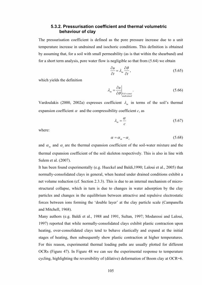
105

5.3.2. Pressurisation coefficient and thermal volumetric behaviour of clay

The pressurisation coefficient is defined as the pore pressure increase due to a unit

temperature increase in undrained and isochoric conditions. This definition is obtained

by assuming that, for a soil with small permeability (as is that within the shearband) and

for a short term analysis, pore water flow is negligible so that from (5.64) we obtain

mut t

θλ∂ ∂=

∂ ∂, (5.65)

which yields the definition

mVol constundrained

uλθ =

∂=∂

. (5.66)

Vardoulakis (2000, 2002a) expresses coefficient mλ in terms of the soil’s thermal

expansion coefficient α and the compressibility coefficient c, as

m cαλ = (5.67)

where:

m cα α α= − (5.68)

and mα and cα are the thermal expansion coefficient of the soil-water mixture and the

thermal expansion coefficient of the soil skeleton respectively. This is also in line with

Sulem et al. (2007).

It has been found experimentally (e.g. Hueckel and Baldi,1990; Laloui et al., 2005) that

normally-consolidated clays in general, when heated under drained conditions exhibit a

net volume reduction (cf. Section 2.3.3). This is due to an internal mechanism of micro-

structural collapse, which in turn is due to changes in water adsorption by the clay

particles and changes in the equilibrium between attractive and repulsive electrostatic

forces between ions forming the ‘double layer’ at the clay particle scale (Campanella

and Mitchell, 1968).

Many authors (e.g. Baldi et al., 1988 and 1991, Sultan, 1997; Modaressi and Laloui,

1997) reported that while normally-consolidated clays exhibit plastic contraction upon

heating, over-consolidated clays tend to behave elastically and expand at the initial

stages of heating, then subsequently show plastic contraction at higher temperatures.

For this reason, experimental thermal loading paths are usually plotted for different

OCRs (Figure 47). In Figure 48 we can see the experimental response to temperature

cycling, highlighting the reversibility of (dilative) deformation of Boom clay at OCR=6.

106

The attainment of a ‘transition temperature’ at which plastic contraction starts in over-

consolidated soils is evident in the change in slope of some of the plots describing

isotropic heating tests at constant confining stress, when the soil’s volumetric behaviour

changes from dilative to contractive (Figure 47 and Figure 49).

As a summary of the important aspects of the thermal volumetric behaviour of clays,

we find it useful to report here the experimental observations by Sultan et al. (2002)

regarding the major thermo-elasto-plastic trends of clay’s behaviour; these are in

agreement with earlier findings (e.g. Demars and Charles, 1982, Baldi et al., 1988):

− The amount of plastic contraction of normally consolidated samples is

independent of the applied mean effective stress;

− Thermal contraction during a test increases when the soil’s OCR is lower,

leading to pure contractive behaviour when OCR=1;

− The slope of the volumetric strain versus temperature curve in the cooling stage

(i.e. the thermo-elastic expansion coefficient) is independent of the applied mean

effective stress;

− The temperature at which transition between thermal expansion and contraction

occurs decreases with OCR.

5.3.2.1. Determination of λm according to Vardoulakis

In light of the above experimental findings, Vardoulakis (2002a) proposes to describe

the thermal volumetric behaviour of clay with a twofold expression for the expansion

coefficient, depending on whether the current temperature is below or above the

transition or “critical” temperature critθ :

if

if

ec crit

c epc crit

α θ θα

α θ θ

⎧ ≤⎪= ⎨>⎪⎩

(5.69)

where ecα denotes the elastic and ep

cα the elasto-plastic thermal expansion coefficients

of the soil skeleton. A constant value for the elastic thermal expansion coefficient is

proposed (slope of A-B in Figure 49) which was found experimentally (Sultan, 1997) to

be practically equal to the thermal expansion coefficient of the soil-water mixture αm,

calculated as

( )1m s wn nα α α= − + . (5.70)

In the above n is the porosity, sα the thermal expansion coefficient of clay particles and

wα that of pore water. Vardoulakis (2002a) suggests that also em cα α≈ (which

107

corresponds to coefficient sβ of Section 4.3), so that at elastic states (i.e. below the

critical temperature), by applying (5.68) the soil’s thermal expansion coefficient

0m cα α α= − = .

At plastic states, by using the additive decomposition of the elasto-plastic coefficient

into elastic and plastic contribution ep e pc c cα α α= + , the thermal expansion coefficient

from Equation (5.68) can be expressed as

( )ep e pc c cα α α α= − − = − (5.71)

where epcα , e

cα and pcα are the elasto-plastic (i.e. slope of B-C in Figure 49), elastic

and plastic expansion coefficients respectively. This leads to the following expression

for the pressurisation coefficient (Vardoulakis 2002a):

0 if

if

crit

pm c

critc

θ θλ α θ θ

≤⎧⎪= ⎨−

>⎪⎩

(5.72)

‘Transition temperature’

Figure 47. Experimentally observed volume changes from isotropic heating tests, at different OCRs, for a kaolin clay (from Laloui and Cekerevac, 2003).

108

Figure 48. From Baldi et al. (1991). Volumetric response of Boom clay to drained isotropic heating/cooling tests, for different OCRs.

‘Transitiontem

perature’

Figure 49. From Vardoulakis (2002a). Isotropic thermal volumetric deformation of an over-consolidated ‘Boom clay’ (OCR=12). The experimental data by Sultan (1997) have been interpolated with a bi-linear law by Vardoulakis (2002a). A-B represents the thermoelastic expansion, at B the ‘transition’ or ‘critical’ temperature is reached after which thermoplastic collapse (B-C) follows. CD represents the cooling phase and shows thermoelastic contraction.

The author also proposes the variation laws with OCR of critical temperature critθ and

plastic contraction coefficient pcα (Vardoulakis, 2002a, equations (27) and (29)), based

on interpolation of the experimental data obtained by Sultan (1997) on the thermal

behaviour of Boom clay (Figure 50). It should be noted here that while for Sultan

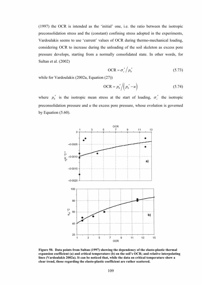
109

(1997) the OCR is intended as the ‘initial’ one, i.e. the ratio between the isotropic

preconsolidation stress and the (constant) confining stress adopted in the experiments,

Vardoulakis seems to use ‘current’ values of OCR during thermo-mechanical loading,

considering OCR to increase during the unloading of the soil skeleton as excess pore

pressure develops, starting from a normally consolidated state. In other words, for

Sultan et al. (2002)

0OCR c pσ ′ ′= (5.73)

while for Vardoulakis (2002a, Equation (27))

( )0 0OCR p p u′ ′= − (5.74)

where 0p ′ is the isotropic mean stress at the start of loading, cσ ′ the isotropic

preconsolidation pressure and u the excess pore pressure, whose evolution is governed

by Equation (5.60).

a)

b)

Figure 50. Data points from Sultan (1997) showing the dependency of the elasto-plastic thermal expansion coefficient (a) and critical temperature (b) on the soil’s OCR; and relative interpolating lines (Vardoulakis 2002a). It can be noticed that, while the data on critical temperature show a clear trend, those regarding the elasto-plastic coefficient are rather scattered.

110

Vardoulakis (2002a), after the above considerations, remarks the yet large uncertainties

in the determination of the value of pressurisation coefficient due to the lack of direct

experimental data and suggests a mean value of 0.06 MPa/°Cmλ = , to be employed

subject to condition (5.72) when the current temperature is above the “critical” one.

5.3.2.2. Determination of λm consistently with the new constitutive model

Within the framework of the constitutive model presented in Chapter 4, the soil’s

thermal behaviour discussed above exhibits some typical features: in purely elastic

conditions the volumetric response of clay to heating is dilative and reversible, and

depends only on coefficient es cβ α= ; in elasto-plastic conditions, the volumetric

response is more complex and is governed by the flow rule (4.11). In this context, the

initial OCR is not a parameter of the problem, but merely an indicator on whether the

state of the soil at the start of loading is elastic or plastic: for a NC soil, further (thermal

or mechanical) loading immediately causes plastic flow, while for an OC soil it initially

causes elastic (reversible) strains until the stress state engages the yield surface.

While Vardoulakis (2002a), in the absence of a constitutive law capable of accounting

for the thermal behaviour of the soil, proposed an expression of mλ based on the

available experimental evidence (Equation (5.72)), this is not an option here. To be

consistent with the thermo-plasticity framework proposed we have to derive the plastic

contraction coefficient (leading to the calculation of mλ according to Equation (5.67))

directly from the assumed constitutive model.

In fact, by definition the thermal expansion (or contraction) coefficient cα in a strain-

temperature constitutive relationship is the factor pre-multiplying the temperature rate:

tepc

d ddt dt

ε θ θε αθ∂

= =∂

(5.75)

where tepε is the thermal contribution to the total thermo-mechanical strain rate

tot tep mepε ε ε= + , (5.76)

and mepε represents the mechanical contribution.

In the elastic regime, coefficient ec cα α= is identified from the elastic volumetric strain

rate expression, as in Equation (4.15), and can be considered either constant, in first

approximation (e.g. the coefficient α used in Mase, 1970, Section 6.9), or pressure- and

temperature-dependent (coefficient βs of Laloui and Cekerevac, 2003). Similarly, at

111

plastic yield the thermo-plastic contraction coefficient tpcα (denoting the thermal only

contribution to the global volumetric strain rate) coincides with the factor pre-

multiplying the temperature rate on the right hand side of the plastic flow expression.

Accordingly, from (4.11) we can write:

( ),pv

fp

λ θ ε ∂=

′∂ε . (5.77)

In the above, the plastic multiplier is given by Equation (5.40), which by substituting

equations (5.41)-(5.43) becomes

( )3 2p v q q s pKf Gf f K f

Hθε ε β θ

λ+ + −

= , (5.78)

where H is specified by (5.47), and the partial derivatives of the yield surface are

expressed by (5.44).

Before elaborating on the above expressions to calculate tpcα , we must impose isotropic

loading conditions in order to be consistent with the experimental evidence and earlier

findings in the literature, as discussed in Section 5.3.2.1. This means prescribing in this

calculation that the stress state must lie at all times on the isotropic axis, at the tip of the

yield envelope, so that

; 0; 0c qp qσ ε′ ′= = = . (5.79)

Substituting conditions (5.79) into (5.78) allows us to reformulate (5.77) as

p mv m vF Fθθ ε= +ε (5.80)

where

22 s pc

f K fF M

Hθ

θ

βσ

−′= (5.81)

is the factor representing the thermal contribution to volumetric plastic strain rates, and

2pm c

KfF M

Hσ ′= (5.82)

represents the isotropic mechanical contribution to volumetric plastic strain rates.

The thermoplastic contraction coefficient is thus equal to factor Fθ . Recalling the

derivatives (5.44) and applying conditions (5.79) yields

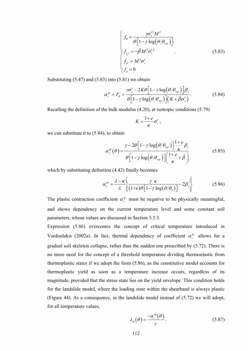
112

( )2 2

2 2

2

1 log

0

pv

c

ref

c

p c

q

Mf

f M

f M

f

θ

ε

γσθ γ θ θ

β σ

σ′

′⎧=⎪ ⎡ ⎤−⎪ ⎣ ⎦

⎪′= −⎨

⎪′=⎪

⎪ =⎩

. (5.83)

Substituting (5.47) and (5.83) into (5.81) we obtain

( )

( ) ( )2 1 log

1 logc ref stp

cref c

KF

Kθ

γσ θ γ θ θ βα

θ γ θ θ βσ

⎡ ⎤′ − −⎣ ⎦= =⎡ ⎤ ′− +⎣ ⎦

. (5.84)

Recalling the definition of the bulk modulus (4.20), at isotropic conditions (5.79)

1c

eK σκ+ ′= ,

we can substitute it to (5.84), to obtain

( )( )

( )

12 1 log

11 log

ref stpc

ref

e

e

γ θ γ θ θ βκα θ

θ γ θ θ βκ

+⎡ ⎤− −⎣ ⎦=

+⎛ ⎞⎡ ⎤− +⎜ ⎟⎣ ⎦ ⎝ ⎠

(5.85)

which by substituting definition (4.42) finally becomes

( ) ( )0

21+e 1 log

tpc s

λ κ γ κα βλ θ γ θ θ

⎧ ⎫− ⎪ ⎪= −⎨ ⎬−⎡ ⎤⎪ ⎪⎣ ⎦⎩ ⎭

(5.86)

The plastic contraction coefficient tpcα must be negative to be physically meaningful,

and shows dependency on the current temperature level and some constant soil

parameters, whose values are discussed in Section 5.5.3.

Expression (5.86) overcomes the concept of critical temperature introduced in

Vardoulakis (2002a). In fact, thermal dependency of coefficient tpcα allows for a

gradual soil skeleton collapse, rather than the sudden one prescribed by (5.72). There is

no more need for the concept of a threshold temperature dividing thermoelastic from

thermoplastic states if we adopt the form (5.86), as the constitutive model accounts for

thermoplastic yield as soon as a temperature increase occurs, regardless of its

magnitude, provided that the stress state lies on the yield envelope. This condition holds

for the landslide model, where the loading state within the shearband is always plastic

(Figure 44). As a consequence, in the landslide model instead of (5.72) we will adopt,

for all temperature values,

( ) ( )tpc

m cα θ

λ θ−

= . (5.87)

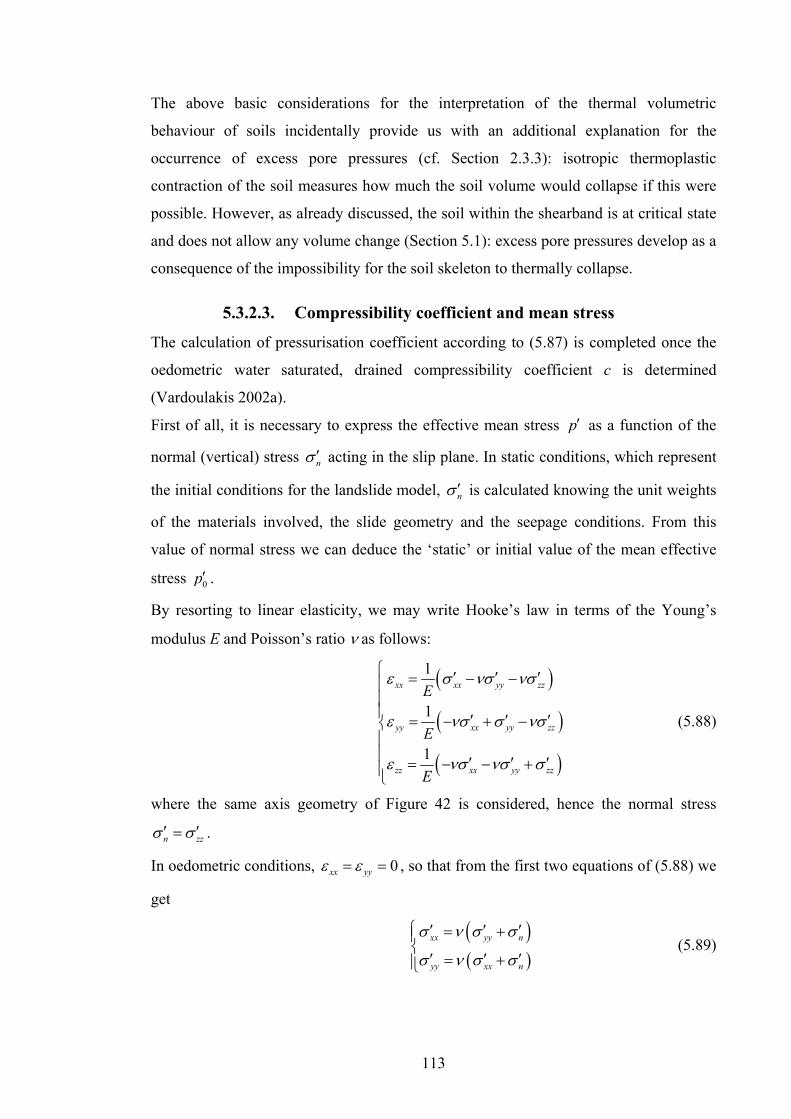
113

The above basic considerations for the interpretation of the thermal volumetric

behaviour of soils incidentally provide us with an additional explanation for the

occurrence of excess pore pressures (cf. Section 2.3.3): isotropic thermoplastic

contraction of the soil measures how much the soil volume would collapse if this were

possible. However, as already discussed, the soil within the shearband is at critical state

and does not allow any volume change (Section 5.1): excess pore pressures develop as a

consequence of the impossibility for the soil skeleton to thermally collapse.

5.3.2.3. Compressibility coefficient and mean stress

The calculation of pressurisation coefficient according to (5.87) is completed once the

oedometric water saturated, drained compressibility coefficient c is determined

(Vardoulakis 2002a).

First of all, it is necessary to express the effective mean stress p′ as a function of the

normal (vertical) stress nσ ′ acting in the slip plane. In static conditions, which represent

the initial conditions for the landslide model, nσ ′ is calculated knowing the unit weights

of the materials involved, the slide geometry and the seepage conditions. From this

value of normal stress we can deduce the ‘static’ or initial value of the mean effective

stress 0p′ .

By resorting to linear elasticity, we may write Hooke’s law in terms of the Young’s

modulus E and Poisson’s ratio ν as follows:

( )

( )

( )

1

1

1

xx xx yy zz

yy xx yy zz

zz xx yy zz

E

E

E

ε σ νσ νσ

ε νσ σ νσ

ε νσ νσ σ

⎧ ′ ′ ′= − −⎪⎪⎪ ′ ′ ′= − + −⎨⎪⎪ ′ ′ ′= − − +⎪⎩

(5.88)

where the same axis geometry of Figure 42 is considered, hence the normal stress

n zzσ σ′ ′= .

In oedometric conditions, 0xx yyε ε= = , so that from the first two equations of (5.88) we

get

( )( )

xx yy n

yy xx n

σ ν σ σ

σ ν σ σ

⎧ ′ ′ ′= +⎪⎨

′ ′ ′= +⎪⎩ (5.89)

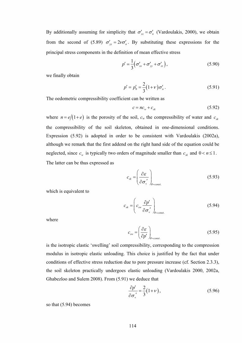
114

By additionally assuming for simplicity that xx nσ σ′ ′= (Vardoulakis, 2000), we obtain

from the second of (5.89) 2yy nσ νσ′ ′= . By substituting these expressions for the

principal stress components in the definition of mean effective stress

( )13 xx yy zzp σ σ σ′ ′ ′ ′= + + , (5.90)

we finally obtain

( )02 13 np p ν σ′ ′ ′= = + . (5.91)

The oedometric compressibility coefficient can be written as

w skc nc c= + (5.92)

where ( )1n e e= + is the porosity of the soil, cw the compressibility of water and skc

the compressibility of the soil skeleton, obtained in one-dimensional conditions.

Expression (5.92) is adopted in order to be consistent with Vardoulakis (2002a),

although we remark that the first addend on the right hand side of the equation could be

neglected, since wc is typically two orders of magnitude smaller than skc and 0 1n< ≤ .

The latter can be thus expressed as

.

sk

v const

cθ

ε

σ=

⎛ ⎞∂= ⎜ ⎟⎜ ⎟′∂⎝ ⎠

(5.93)

which is equivalent to

.

sk sw

v const

pc cθ

σ=

⎛ ⎞′∂= ⎜ ⎟⎜ ⎟′∂⎝ ⎠

(5.94)

where

.

swconst

cp θ

ε

=

⎛ ⎞∂= ⎜ ⎟′∂⎝ ⎠

(5.95)

is the isotropic elastic ‘swelling’ soil compressibility, corresponding to the compression

modulus in isotropic elastic unloading. This choice is justified by the fact that under

conditions of effective stress reduction due to pore pressure increase (cf. Section 2.3.3),

the soil skeleton practically undergoes elastic unloading (Vardoulakis 2000, 2002a,

Ghabezloo and Sulem 2008). From (5.91) we deduce that

( )2 13

v

p νσ

′∂= +

′∂, (5.96)

so that (5.94) becomes

115

( )2 13sk swc cν= + (5.97)

In order to calculate (5.95) consistently with the proposed constitutive framework, we

may resort to the equation of the soil’s unloading-reloading line (URL) in the ( )ln , vp′

compression plane:

( )0v v ln pκ ′= − (5.98)

where ( )v 1 e= + is the specific volume, so that

vddp p

κ= −′ ′

. (5.99)

Since an increment in specific volume produces an increment of volumetric strain

vvv

ddε = − (5.100)

(see e.g. Muir Wood, 1990), where the negative sign comes from the soil mechanics

convention that compressive strains are positive, we may substitute definition

v v vd dε= − ⋅ into (5.99), to obtain

( )v 1

vswc

p p e pε κ κ∂

= = =′ ′ ′∂ +

(5.101)

where we can set as mean effective stress in the shearband the static value, 0p p′ ′= .

By substituting (5.97) and (5.101) into (5.92), compressibility takes the form

( )( )0

2 11 3 1

wec c

e p e

κ ν+⎛ ⎞= +⎜ ⎟+ ′⎝ ⎠ +. (5.102)

5.4. Dynamical equation

The dynamical equation describes the time evolution of the landslide velocity (see also

Section 2.3.4.2), when the soil mass is assumed to rotate as a rigid body with respect to

the centre of a previously defined critical failure circle. By calculating the net driving

moment of the mass assuming a constant normal stress (set equal to a mean value)

acting along the whole failure circle, the linear acceleration of the slide can be

expressed as (Vardoulakis, 2002a):

( ) ( )( )

20

ddm

c m

u tdv R Adt p

ω μμ

⎛ ⎞= +⎜ ⎟⎜ ⎟

⎝ ⎠. (5.103)

Parameter A is expressed as

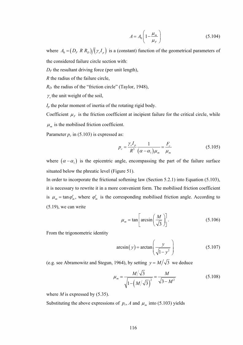
116

0 1 m

F

A A μμ

⎛ ⎞= −⎜ ⎟

⎝ ⎠ (5.104)

where ( ) ( )0 F D s pA D R R Iγ= is a (constant) function of the geometrical parameters of

the considered failure circle section with:

DF the resultant driving force (per unit length),

R the radius of the failure circle,

RD the radius of the “friction circle” (Taylor, 1948),

sγ the unit weight of the soil,

Ip the polar moment of inertia of the rotating rigid body.

Coefficient Fμ is the friction coefficient at incipient failure for the critical circle, while

mμ is the mobilised friction coefficient.

Parameter pc in (5.103) is expressed as:

( )3

1

1s p cc

m m

I FpRγ

α α μ μ= =

− (5.105)

where ( )1α α− is the epicentric angle, encompassing the part of the failure surface

situated below the phreatic level (Figure 51).

In order to incorporate the frictional softening law (Section 5.2.1) into Equation (5.103),

it is necessary to rewrite it in a more convenient form. The mobilised friction coefficient

is tanm mμ ϕ′= , where mϕ′ is the corresponding mobilised friction angle. According to

(5.19), we can write

tan arcsin3m

Mμ⎡ ⎤⎛ ⎞= ⎢ ⎥⎜ ⎟

⎝ ⎠⎣ ⎦. (5.106)

From the trigonometric identity

( )2

arcsin arctan1

yyy

⎛ ⎞⎜ ⎟=⎜ ⎟−⎝ ⎠

(5.107)

(e.g. see Abramowitz and Stegun, 1964), by setting 3y M= we deduce

( )2 2

331 3

mM M

MMμ = =

−− (5.108)

where M is expressed by (5.35).

Substituting the above expressions of pc, A and mμ into (5.103) yields

117

2 00 0 23

d d

F c

dv A uMR Adt FM

ωμ

⎡ ⎤⎛ ⎞= − +⎢ ⎥⎜ ⎟

− ⎝ ⎠⎣ ⎦ (5.109)

where ( ),d z du u z t

== . This is the last one of the set of governing equations for the

landslide model, summarised below:

( )2

2

2

2

2 00 0 2

(I)

(II)

(III) 3

di i

v m

d d

F c

v tD F

t z du uct z t

dv A uMR Adt FM

θ θ

θλ

ωμ

⎧ ∂ ∂⎪ = +∂ ∂⎪

⎪ ∂ ∂ ∂⎪ = +⎨ ∂ ∂ ∂⎪⎪ ⎡ ⎤⎛ ⎞

= − +⎪ ⎢ ⎥⎜ ⎟−⎪ ⎝ ⎠⎣ ⎦⎩

. (5.110)

Figure 51. From Vardoulakis (2002a). Critical failure circle for ‘section 6’ of the Vajont slide. The epicentric angle represents the immersed part of the circular failure surface, and corresponds to the portion α- α1=(37°-11°) in this case.

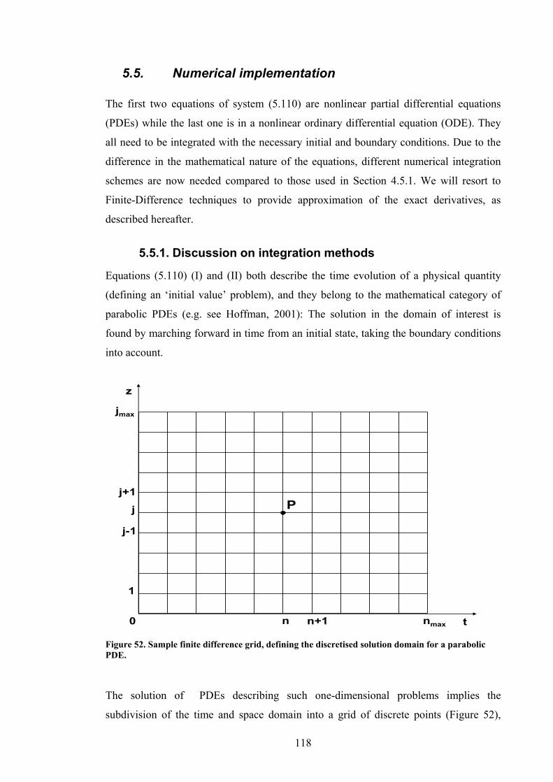
118

5.5. Numerical implementation

The first two equations of system (5.110) are nonlinear partial differential equations

(PDEs) while the last one is in a nonlinear ordinary differential equation (ODE). They

all need to be integrated with the necessary initial and boundary conditions. Due to the

difference in the mathematical nature of the equations, different numerical integration

schemes are now needed compared to those used in Section 4.5.1. We will resort to

Finite-Difference techniques to provide approximation of the exact derivatives, as

described hereafter.

5.5.1. Discussion on integration methods

Equations (5.110) (I) and (II) both describe the time evolution of a physical quantity

(defining an ‘initial value’ problem), and they belong to the mathematical category of

parabolic PDEs (e.g. see Hoffman, 2001): The solution in the domain of interest is

found by marching forward in time from an initial state, taking the boundary conditions

into account.

z

tn n+10

1

j

j-1

j+1

nmax

jmax

P

Figure 52. Sample finite difference grid, defining the discretised solution domain for a parabolic PDE.

The solution of PDEs describing such one-dimensional problems implies the

subdivision of the time and space domain into a grid of discrete points (Figure 52),

119

where the derivatives entering the problem are to be calculated. Similarly to those for

ODEs (Section 4.5.1), existing integration methods for parabolic PDEs can be

subdivided into explicit and implicit ones.

In explicit methods, the solution at a point P at time step n+1 depends only on the

solution at neighbouring points at the previous time step n. Thus, at each integration

step a small triangular area of the integration domain is involved in the calculation

(‘numerical domain of dependence’ in Figure 53). In implicit methods, on the other

hand, the solution at point P at time step n+1 depends on the solution at neighbouring

points, both at time step n+1 and time step n. The numerical domain of dependence is in

this case extended to the whole spatial range enclosed by time levels n and n+1 (Figure

54). While explicit methods involve the solution of a single equation in terms of known

quantities, implicit ones require the solution of a system of equations to be found at

each time-step.

Among the available methods, we consider three potentially suitable ones for the

discretisation of equations (5.110):

• Forward-time centred-space (FTCS), explicit

• Backward-time centred-space (BTCS), implicit

• Crank-Nicholson (CN), implicit.

The FTCS method provides a first-order approximation in time and second-order

approximation in space (cf. Section 4.5.1). This method is very straightforward to

implement, as it does not require the solution of a system, implying less computational

expense. However, stability is not guaranteed for explicit methods and a restriction in

the size of the time-step is needed. In other words, the solution might not be bounded if

the time-step is bigger than a threshold value, to be established through an appropriate

stability analysis (e.g. see Press, 1988). The BTCS method overcomes this difficulty, as

all implicit methods are unconditionally stable, despite requiring a fairly larger

computational effort in order to handle the more complex algebra. The CN method still

retains the stability advantages of BTCS, and improves on the accuracy since it provides

a second-order approximation in time. The mathematical formulation here is more

complicated, but the overall robustness is an undoubted advantage that would make this

method the most suitable one for discretising equations (5.110). Nevertheless, the

convenience of adopting CN should be reconsidered in light of the potential

nonlinearity of the considered equations. In our case, equations (5.110) contain

nonlinear terms as discussed in Sections 5.2 and 5.3.2, which constitute a considerable

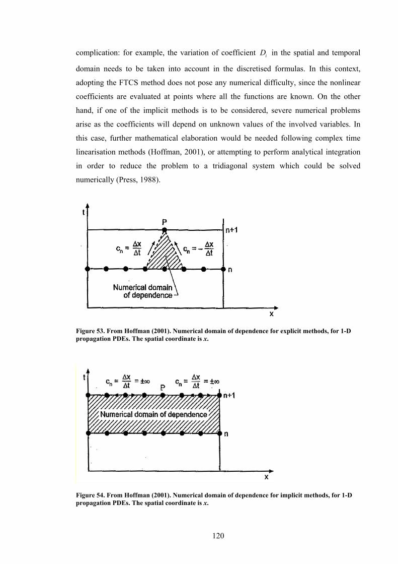
120

complication: for example, the variation of coefficient iD in the spatial and temporal

domain needs to be taken into account in the discretised formulas. In this context,

adopting the FTCS method does not pose any numerical difficulty, since the nonlinear

coefficients are evaluated at points where all the functions are known. On the other

hand, if one of the implicit methods is to be considered, severe numerical problems

arise as the coefficients will depend on unknown values of the involved variables. In

this case, further mathematical elaboration would be needed following complex time

linearisation methods (Hoffman, 2001), or attempting to perform analytical integration

in order to reduce the problem to a tridiagonal system which could be solved

numerically (Press, 1988).

Figure 53. From Hoffman (2001). Numerical domain of dependence for explicit methods, for 1-D propagation PDEs. The spatial coordinate is x.

Figure 54. From Hoffman (2001). Numerical domain of dependence for implicit methods, for 1-D propagation PDEs. The spatial coordinate is x.

121

In conclusion, the presence of nonlinear coefficients, in addition to the existence of

several couplings in equations (5.110), incline us to adopt the FTCS method. In fact, the

additional effort of performing a stability analysis (strongly recommended for explicit

methods) is largely compensated by the mathematical and numerical simplifications that

explicit integration implies, compared to implicit methods.

5.5.2. Discretisation

The heat Equation (5.110)-(I) can be discretised with a FTCS scheme as

( )

11 1

2

2n n n n n nj j j j jn n d

j jvD F

t dz

θ θ θ θ θ++ −− − +

= +Δ Δ

(5.111)

where the subscripts denote the spatial position, superscripts the time value (Figure 52),

tΔ the time-step and zΔ the spatial step amplitude. The ‘current’ values of space and

time are respectively j and n. Since the involved coefficients are not constant but depend

on the current values of temperature, pore pressure and velocity we have

( ) ( ), , ; , ,n n n n n n n nj i j j d j i j j dD D u v F F u vθ θ= = . (5.112)

Similarly, the pore pressure Equation (5.110)-(II) can be approximated as

( )

1 11 1

2

2n n n n n n nj j j j j j jn

v j

u u u u uc

t tz

θ θλ

+ ++ −− − + −

= +Δ ΔΔ

(5.113)

where (5.111) can be substituted, to provide the finite difference approximation of the

temperature rate. The same grid notation as above applies, coefficient vc is taken

constant and the pressurisation coefficient as shown in Section 5.3.2 depends on the

current value of temperature:

( )n nj m jλ λ θ= . (5.114)

The dynamical equation is a uni-dimensional ODE and describes the variation over time

of the problem quantities, while the spatial coordinate is fixed to the shearband-rigid

block interface (z=d). Equation (5.110)-(III) can therefore be discretised using a

standard 4th order Runge-Kutta (RK) method (Section 4.5.1). By defining the value of

the time-derivative of the slide velocity (RHS of Equation (5.109)) at the generic time-

step i as

( )( )

2 00 0 2

, ,

3 , ,

i i i id d di d

i i i F cd d d

M x v A uf R AFM x v

θω

μθ

⎡ ⎤⎛ ⎞⎢ ⎥

= − +⎜ ⎟⎢ ⎥⎝ ⎠⎡ ⎤⎢ ⎥− ⎣ ⎦⎣ ⎦

, (5.115)

we may write the 4th order RK approximation as

122

1

1 2 11 2 16 3 6

n nn n nd dv v f f f

t

++ +−

= + +Δ

(5.116)

where the variables at halfway time-step ( )1 2n + , if the step size is reasonably small,

may be logically calculated as ( )1/ 2 112

n n nd d dθ θ θ+ += + , ( )1/ 2 11

2n n nd d du u u+ += + and so on.

Equations (5.111), (5.113) and (5.116) can be integrated numerically in this same order,

since despite the numerous couplings they may be solved explicitly in sequence: the

first equation provides the value of 1njθ+ , which is used in the second one to obtain the

solution for 1nju + . Both values can then be used into the dynamical equation to find the

slide velocity 1ndv + .

The numerical procedure for solving Equation (5.116) depends on the kind of friction

softening adopted: if all dependencies of the friction-softening law are taken into

account, (5.116) becomes a nonlinear algebraic equation which must be solved

iteratively (Section 5.5.7.3). If on the contrary we ignore the displacement and velocity

dependence of parameter M, we may solve the equation directly (Section 5.5.7.2).

5.5.3. Choice of parameters for the Vajont case study

As an example we back-analyse the Vajont case with the modified landslide model, to

asses its consistency with the available field observations and the calculations

performed by Vardoulakis (2002a). The constant material and system parameters for our

calculations are hence chosen, where possible, consistently with Vardoulakis (2002a).

Our analysis will be hereafter carried out for ‘Section 5’ of the Vajont slide, whose

parameters are summarised in Table 4.

The implementation of the thermoplastic model introduces a few additional parameters

compared to Vardoulakis (2002a) which are separately discussed hereafter.

5.5.3.1. Void ratio

The void ratio at critical state e is calculated through the more conventional critical state

soil parameter Γ, representing the soil’s specific volume intercept at unit mean effective

stress equal to 1 kPa. The CSL in the v-ln(p’) plane is expressed as

v (1 ) lncs cse pλ ′= + = Γ − (5.117)

(e.g. Powrie, 1997) so that we may calculate

1 ln( )cse pλ ′= Γ − − (5.118)

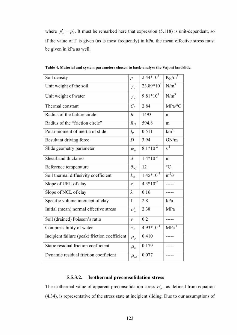
123

where 0csp p′ ′= . It must be remarked here that expression (5.118) is unit-dependent, so

if the value of Γ is given (as is most frequently) in kPa, the mean effective stress must

be given in kPa as well.

Table 4. Material and system parameters chosen to back-analyse the Vajont landslide.

Soil density ρ 2.44*103 Kg/m3

Unit weight of the soil sγ 23.89*103 N/m3

Unit weight of water wγ 9.81*103 N/m3

Thermal constant Cf 2.84 MPa/°C

Radius of the failure circle R 1493 m

Radius of the “friction circle” RD 594.8 m

Polar moment of inertia of slide Ip 0.511 km4

Resultant driving force D 3.94 GN/m

Slide geometry parameter 0ω 8.1*10-2 s-1

Shearband thickness d 1.4*10-3 m

Reference temperature θref 12 °C

Soil thermal diffusivity coefficient km 1.45*10-7 m2/s

Slope of URL of clay κ 4.3*10-2 -----

Slope of NCL of clay λ 0.16 -----

Specific volume intercept of clay Γ 2.8 kPa

Initial (mean) normal effective stress nσ ′ 2.38 MPa

Soil (drained) Poisson’s ratio ν 0.2 -----

Compressibility of water cw 4.93*10-4 MPa-1

Incipient failure (peak) friction coefficient pμ 0.410 -----

Static residual friction coefficient rsμ 0.179 -----

Dynamic residual friction coefficient rdμ 0.077 -----

5.5.3.2. Isothermal preconsolidation stress

The isothermal value of apparent preconsolidation stress mσ ′ , as defined from equation

(4.34), is representative of the stress state at incipient sliding. Due to our assumptions of

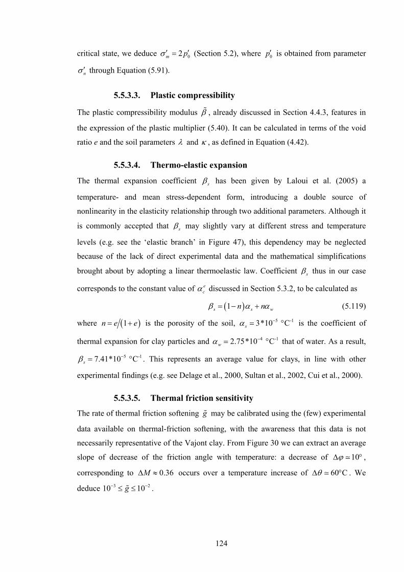
124

critical state, we deduce 02m pσ ′ ′= (Section 5.2), where 0p′ is obtained from parameter

nσ ′ through Equation (5.91).

5.5.3.3. Plastic compressibility

The plastic compressibility modulus β , already discussed in Section 4.4.3, features in

the expression of the plastic multiplier (5.40). It can be calculated in terms of the void

ratio e and the soil parameters λ and κ , as defined in Equation (4.42).

5.5.3.4. Thermo-elastic expansion

The thermal expansion coefficient sβ has been given by Laloui et al. (2005) a

temperature- and mean stress-dependent form, introducing a double source of

nonlinearity in the elasticity relationship through two additional parameters. Although it

is commonly accepted that sβ may slightly vary at different stress and temperature

levels (e.g. see the ‘elastic branch’ in Figure 47), this dependency may be neglected

because of the lack of direct experimental data and the mathematical simplifications

brought about by adopting a linear thermoelastic law. Coefficient sβ thus in our case

corresponds to the constant value of ecα discussed in Section 5.3.2, to be calculated as

( )1s s wn nβ α α= − + (5.119)

where ( )1n e e= + is the porosity of the soil, 5 -13*10 Csα−= ° is the coefficient of

thermal expansion for clay particles and 4 -12.75*10 Cwα−= ° that of water. As a result,

5 -17.41*10 Csβ−= ° . This represents an average value for clays, in line with other

experimental findings (e.g. see Delage et al., 2000, Sultan et al., 2002, Cui et al., 2000).

5.5.3.5. Thermal friction sensitivity

The rate of thermal friction softening g may be calibrated using the (few) experimental

data available on thermal-friction softening, with the awareness that this data is not

necessarily representative of the Vajont clay. From Figure 30 we can extract an average

slope of decrease of the friction angle with temperature: a decrease of 10ϕΔ ° ,

corresponding to 0.36MΔ ≈ occurs over a temperature increase of 60 CθΔ ° . We

deduce 3 210 10g− −≤ ≤ .

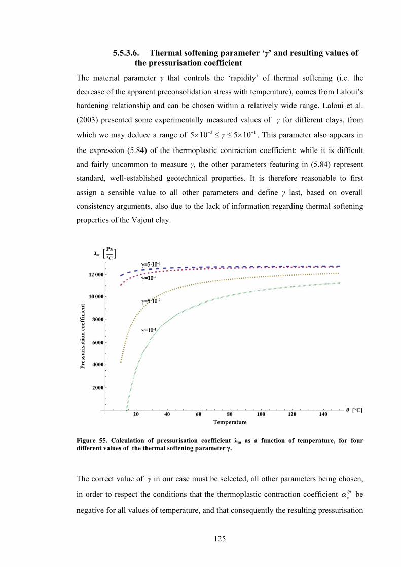
125

5.5.3.6. Thermal softening parameter ‘γ’ and resulting values of the pressurisation coefficient

The material parameter γ that controls the ‘rapidity’ of thermal softening (i.e. the

decrease of the apparent preconsolidation stress with temperature), comes from Laloui’s

hardening relationship and can be chosen within a relatively wide range. Laloui et al.

(2003) presented some experimentally measured values of γ for different clays, from

which we may deduce a range of 3 15 10 5 10γ− −× ≤ ≤ × . This parameter also appears in

the expression (5.84) of the thermoplastic contraction coefficient: while it is difficult

and fairly uncommon to measure γ, the other parameters featuring in (5.84) represent

standard, well-established geotechnical properties. It is therefore reasonable to first

assign a sensible value to all other parameters and define γ last, based on overall

consistency arguments, also due to the lack of information regarding thermal softening

properties of the Vajont clay.

γ=5∙10‐3

γ=10‐2

γ=5∙10‐2

γ=10‐1

Temperature

Pressurisationcoefficient

Figure 55. Calculation of pressurisation coefficient λm as a function of temperature, for four different values of the thermal softening parameter γ.

The correct value of γ in our case must be selected, all other parameters being chosen,

in order to respect the conditions that the thermoplastic contraction coefficient tpcα be

negative for all values of temperature, and that consequently the resulting pressurisation

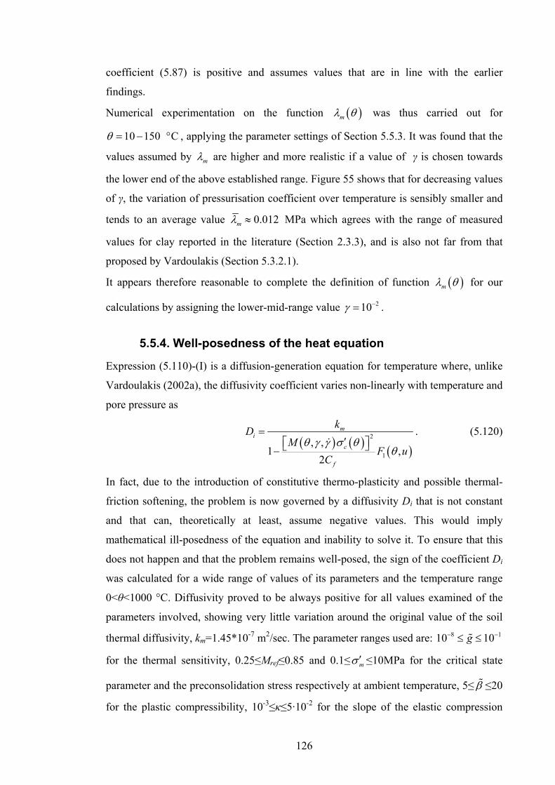
126

coefficient (5.87) is positive and assumes values that are in line with the earlier

findings.

Numerical experimentation on the function ( )mλ θ was thus carried out for

10 150 Cθ = − ° , applying the parameter settings of Section 5.5.3. It was found that the

values assumed by mλ are higher and more realistic if a value of γ is chosen towards

the lower end of the above established range. Figure 55 shows that for decreasing values

of γ, the variation of pressurisation coefficient over temperature is sensibly smaller and

tends to an average value 0.012mλ ≈ MPa which agrees with the range of measured

values for clay reported in the literature (Section 2.3.3), and is also not far from that

proposed by Vardoulakis (Section 5.3.2.1).

It appears therefore reasonable to complete the definition of function ( )mλ θ for our

calculations by assigning the lower-mid-range value 210γ −= .

5.5.4. Well-posedness of the heat equation

Expression (5.110)-(I) is a diffusion-generation equation for temperature where, unlike

Vardoulakis (2002a), the diffusivity coefficient varies non-linearly with temperature and

pore pressure as

( ) ( ) ( )

2

1

, ,1 ,

2

mi

c

f

kDM

F uC

θ γ γ σ θθ

=′⎡ ⎤⎣ ⎦−

. (5.120)

In fact, due to the introduction of constitutive thermo-plasticity and possible thermal-

friction softening, the problem is now governed by a diffusivity Di that is not constant

and that can, theoretically at least, assume negative values. This would imply

mathematical ill-posedness of the equation and inability to solve it. To ensure that this

does not happen and that the problem remains well-posed, the sign of the coefficient Di

was calculated for a wide range of values of its parameters and the temperature range

0<θ<1000 °C. Diffusivity proved to be always positive for all values examined of the

parameters involved, showing very little variation around the original value of the soil

thermal diffusivity, km=1.45*10-7 m2/sec. The parameter ranges used are: 8 110 10g− −≤ ≤

for the thermal sensitivity, 0.25≤Mref≤0.85 and 0.1≤ mσ ′ ≤10MPa for the critical state

parameter and the preconsolidation stress respectively at ambient temperature, 5≤β ≤20

for the plastic compressibility, 10-3≤κ≤5·10-2 for the slope of the elastic compression

127

line, 0.15≤ν≤0.45 for the Poisson’s ratio, 0.2≤e≤1.5 for the void ratio and 0.005≤γ≤0.5

for the parameter-γ of the thermoplastic model. In Figure 56 an example of this

calculation for the given temperature range, at mid-range values of the involved

parameters, is shown.

Di (m2/s)

θ (°C)

0.005 0.5γ = −

8 110 10g − −= −0.25 0.85refM = −

0.1 10 MPamσ′ = −5 20β = −

3 210 5 10k − −= − ⋅0.15 0.45ν = −0.2 1.5e = −

Figure 56. Calculation of the sign of coefficient Di for mid-range values of involved parameters (whose typical ranges are listed in the framed box) and temperature ranging between 0 and 1000 °C.

5.5.5. Time-step analysis

As mentioned in Section 5.5.1, the explicit integration scheme employed will be

numerically unstable if the adopted time-step tΔ is larger than a limit value. A stability

analysis is recommended whenever explicit schemes are employed.

Among the various techniques available for performing stability analysis of a finite

difference approximation of a PDE, the von Neumann method (e.g. see Hoffman, 2002)

is one of the simplest and most widely used. For a 1-D parabolic equation having the

general form like the heat and pore pressure equations at hand,

( ) ( )2

2, ,f fz t g z tt z

β∂ ∂= +

∂ ∂ (5.121)

128

where f is the considered variable, z the spatial coordinate, β the diffusivity and g the

source (generation) term, the corresponding finite difference scheme (cf. Section 5.5.2)

is

( )

11 1

2

n n n n nj j j j jn n

j j

f f f f fg

t zβ

++ −− − +

= +Δ Δ

. (5.122)

The stability condition of the finite difference scheme (5.122) based on the von

Neumann stability analysis is (e.g. see Press, 1988)

( )2

2z

tβ

ΔΔ ≤ . (5.123)

However, the above stability criterion applies to linear PDEs only (Hoffman, 2002), i.e.

when constantnjβ β= = , while nonlinear PDEs need a more complex local linearisation

procedure before being analysed for stability.

Since in our case the governing equations are formally nonlinear, as a first check we

performed some numerical experimentation, by identifying a threshold value for tΔ (at

given xΔ ) below which the numerical results are unaffected by changes in time-step.

For the Vajont back-analysis calculations, a safe, small enough value of the time-step,

for the chosen spatial resolution of 0.02mmzΔ = was found to be 410t −Δ = s.

Nevertheless, by taking a closer look at the results we notice that the coefficients

featuring in the PDEs are constant or virtually so. In fact, on Section 5.3.1 we have

chosen to take the consolidation coefficient vc constant, given the weakness of its

temperature dependence. Moreover, in Section 5.5.4 we have shown the minor

variability of the diffusivity Di: since its magnitude of variation is of the order of 10-12

along a 1000°C temperature span (Figure 56), this coefficient remains for all practical

purposes equal to the original thermal diffusivity value of km=1.45*10-7, i.e. i mD k≅ . In

this context, the need for local linearization disappears and we may directly carry out a

stability analysis, to decide the maximum time-step size that can be employed whilst

respecting condition (5.123).

For the finite difference pore pressure Equation (5.113), the stability condition becomes

( )2

2 v

zt

cΔ

Δ ≤ (5.124)

where vc has the form (5.61) and the spatial step zΔ , for practical purposes, in our

numerical code is a function of the imposed shearband thickness d, z d wΔ = where w

is the (integer) number of spatial subdivisions desired within the shearband thickness.

129

For the finite difference heat Equation (5.111), the stability condition is

( )2

2 m

zt

kΔ

Δ ≤ (5.125)

where zΔ is the same as in (5.124).

The time-step choice is then defined by the condition

( ) ( )2 2

max min ,2 2m v

z zt

k c

⎡ ⎤Δ ΔΔ ≤ ⎢ ⎥

⎢ ⎥⎣ ⎦. (5.126)

By substituting into (5.126) the values chosen for Vajont of -30.02 10zΔ = × m, 7 21.45 10 m smk −= × and 8 27.3 10 m svc −= × (Section 5.3.1) we obtain

3max 10t −Δ ≤

which confirms that indeed the ‘safe’ value 410t −Δ = found through numerical

experimentation respects the stability criterion.

5.5.6. Initial and boundary conditions

The finite difference equations (Section 5.5.2) are integrated in a spatial domain

composed of the shearband thickness and the surrounding clayey soil. In fact, as

anticipated in Section 2.1.4.1 the shearband is assumed to be embedded in a clay layer

of the same characteristics, whose thickness is much larger than the band dimensions. In

other words, the band merely marks the boundaries of strain localisation, in an

otherwise thicker clayey layer. Shear strain and consequent heat production will occur

within the localisation band only. The 1-D spatial domain is here set to be 10 times the

thickness of the shearband and assumed to be uniform in hydraulic and geotechnical

properties. In line with Vardoulakis (2002a), the assumption is made that at large

distance from the band (i.e. at the domain boundaries) the excess pore pressure is zero

and the temperature is equal to the ambient one:

( ) ( ), 0; , refu t tθ θ±∞ = ±∞ = . (5.127)

The velocity profile through the thickness domain (as discussed in Section 2.3.4.1, see

Figure 57) is defined as:

[ ]

( ) [ ]

( ) [ ]

0 z - ,0zt z 0,d

t z ,

d

d

v

v v d

v v d

⎧ = ∈ ∞⎪⎪ = ∈⎨⎪⎪ = ∈ +∞⎩

. (5.128)

Initial conditions are:

130

( ) ( ) ( ),0 ; ,0 0; ,0 0refz u z v zθ θ= = = . (5.129)

In order to initiate the movement, the sliding mass needs to be unbalanced from its limit

equilibrium. This can be achieved numerically by assuming an arbitrarily small

reduction of the limit equilibrium friction angle. Following Vardoulakis (2002a), such

reduction is chosen to be of 0.1%.

For a time window of 10 seconds after movement initiation, corresponding to a

computed value of displacement not exceedingly large ( 120mdx < ) so that the

assumption of rigid-body remains reasonable, the model equations were integrated

numerically. Results are presented hereafter.

z

t

d Strain localisationthickness domain

Tota

l thi

ckne

ssdo

mai

n=10

*dRigid body (in motion)

Rigid body (still)

Figure 57. Finite difference grid showing the thickness domain of integration. The shearband is a strain localisation zone of thickness d, embedded in an otherwise homogeneous soil layer of total thickness 10d. The soil below the shearband is still, while the soil at the top of the shearband moves at the velocity vd, characteristic of the landslide overburden.

5.5.7. Numerical results for Vajont

5.5.7.1. Vaporisation threshold

Before starting the computations, we should here remark that our model ceases to be

valid as soon as the temperature within the shearband reaches the evaporation limit of

the pore water for the current pressure. After this transition point, the governing

equations would need substantial modifications since the energy balance should account

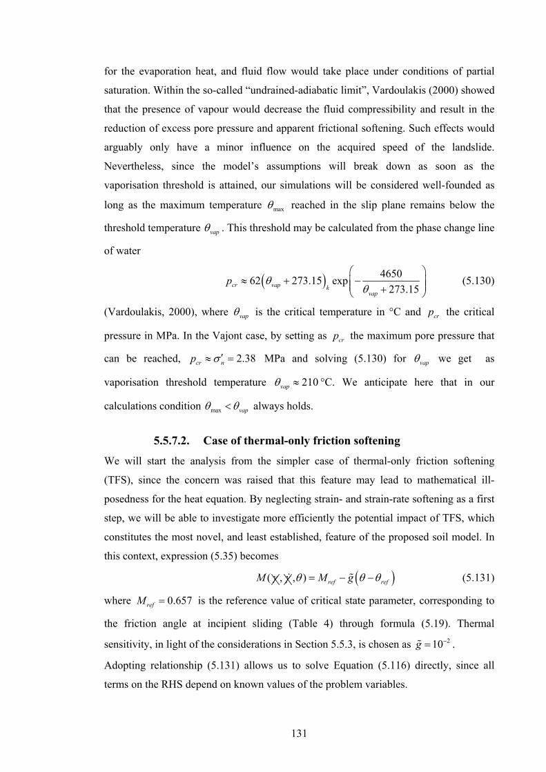
131

for the evaporation heat, and fluid flow would take place under conditions of partial

saturation. Within the so-called “undrained-adiabatic limit”, Vardoulakis (2000) showed

that the presence of vapour would decrease the fluid compressibility and result in the

reduction of excess pore pressure and apparent frictional softening. Such effects would

arguably only have a minor influence on the acquired speed of the landslide.

Nevertheless, since the model’s assumptions will break down as soon as the

vaporisation threshold is attained, our simulations will be considered well-founded as

long as the maximum temperature maxθ reached in the slip plane remains below the

threshold temperature vapθ . This threshold may be calculated from the phase change line

of water

( ) 465062 273.15 exp273.15cr vap k

vap

p θθ

⎛ ⎞≈ + −⎜ ⎟⎜ ⎟+⎝ ⎠

(5.130)

(Vardoulakis, 2000), where vapθ is the critical temperature in °C and crp the critical

pressure in MPa. In the Vajont case, by setting as crp the maximum pore pressure that

can be reached, 2.38cr np σ ′≈ = MPa and solving (5.130) for vapθ we get as

vaporisation threshold temperature 210vapθ ≈ °C. We anticipate here that in our

calculations condition max vapθ θ< always holds.

5.5.7.2. Case of thermal-only friction softening

We will start the analysis from the simpler case of thermal-only friction softening

(TFS), since the concern was raised that this feature may lead to mathematical ill-

posedness for the heat equation. By neglecting strain- and strain-rate softening as a first

step, we will be able to investigate more efficiently the potential impact of TFS, which

constitutes the most novel, and least established, feature of the proposed soil model. In

this context, expression (5.35) becomes

( )( , , ) ref refM M gγ γ θ θ θ= − − (5.131)

where 0.657refM = is the reference value of critical state parameter, corresponding to

the friction angle at incipient sliding (Table 4) through formula (5.19). Thermal

sensitivity, in light of the considerations in Section 5.5.3, is chosen as 210g −= .

Adopting relationship (5.131) allows us to solve Equation (5.116) directly, since all

terms on the RHS depend on known values of the problem variables.

132

With these settings, temperature and pore pressure were computed at each grid-point of

the spatial domain, and isochrones through the domain were produced at significant

time values (Figure 58 and Figure 59). It can be seen that temperature inside the

shearband reaches about 145 °C after 10 seconds (about 8 seconds after the outbreak of

acceleration, as can be seen from the velocity profile in Figure 60). This is well below

the water vaporisation threshold at the given pressure, as pointed out in Section 5.5.7.1.

The overburden corresponds to an initial vertical effective stress of 2.38 MPa which, as

a consequence of the effective stress principle, is also the maximum value that excess

pore pressure can reach. It can be seen that this value is approached as excess pore

pressures overtops 2 MPa after 10 s from slide triggering.

In Figure 60 and Figure 61 the corresponding computed slide velocity and displacement

are plotted. From the velocity plot we can distinguish the slide ‘triggering point’ (at t=0,

due to the 0.1% reduction of the incipient failure friction angle, cf. Section 5.5.6) and

the slide’s (catastrophic) ‘activation point’, here set at 1.8 st ≈ , when the acceleration

of the mass abruptly increases. In fact, the velocity profile shows negligible increase up

to 2t s, followed by a rapid kick at 3t s which corresponds to a substantial increase

in the pressurisation rate, as can be seen in Figure 59.

( )M M θ=

Figure 58. Temperature isochrones within the shearband and its surroundings, for the case of thermal-only friction softening. The shearband area, where strain localisation takes place, is shaded.

133

( )M M θ=

Figure 59. Pore pressure isochrones within the shearband and its surroundings, for the case of thermal-only friction softening. The shearband area, where strain localisation takes place, is shaded.

0 1 2 3 4 5 6 7 8 9 100

5

10

15

20

25landslide velocity

time (s)

velo

city

vd (m

/s)

Figure 60. Slide velocity profile for the case of thermal-only friction softening.

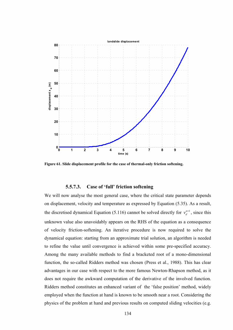
134

0 1 2 3 4 5 6 7 8 9 100

10

20

30

40

50

60

70

80landslide displacement

time (s)

disp

lace

men

t xd (m

)

Figure 61. Slide displacement profile for the case of thermal-only friction softening.

5.5.7.3. Case of ‘full’ friction softening

We will now analyse the most general case, where the critical state parameter depends

on displacement, velocity and temperature as expressed by Equation (5.35). As a result,

the discretised dynamical Equation (5.116) cannot be solved directly for 1ndv + , since this

unknown value also unavoidably appears on the RHS of the equation as a consequence

of velocity friction-softening. An iterative procedure is now required to solve the

dynamical equation: starting from an approximate trial solution, an algorithm is needed

to refine the value until convergence is achieved within some pre-specified accuracy.

Among the many available methods to find a bracketed root of a mono-dimensional

function, the so-called Ridders method was chosen (Press et al., 1988). This has clear

advantages in our case with respect to the more famous Newton-Rhapson method, as it

does not require the awkward computation of the derivative of the involved function.

Ridders method constitutes an enhanced variant of the ‘false position’ method, widely

employed when the function at hand is known to be smooth near a root. Considering the

physics of the problem at hand and previous results on computed sliding velocities (e.g.

135

Vardoulakis, 2002a), we can reasonably assert that ( )dv t is a growing function of time,

so that at each step we may easily set two bracketing values, Lv and Rv within which

the new value of velocity 1ndv + lies: the previous value ( n

L dv v= ), and a reasonably

higher value ( 10 nR dv v= ⋅ ). Numerical implementation of this method ensured

convergence in a few iteration steps.

In Figure 62 and Figure 63 the temperature and pore pressure isochrones are plotted for

this case of ‘full’ friction softening (FFS), in Figure 64 and Figure 65 the velocity and

displacement profiles are plotted for a time window of 10 seconds after triggering. In

comparison with the TFS case, we can observe that:

• Sliding is activated earlier here (after about half a second from triggering as

opposed to 2∼ seconds in TFS case, as can be seen by comparing Figure 64 and

Figure 60), as a result of the ‘full’ softening law providing a quicker decrease of

the friction angle alongside temperature, displacement and velocity.

• A higher final velocity is reached, v(t=10s)=26.3 m/s as opposed to 21 m/s in TFS

case. This depends on the above mentioned earlier ‘activation’ of the slide,

implying a longer overall time of catastrophic sliding for the FFS case. For the

same reason, also displacement after 10 seconds is substantially larger (119.5 m)

• A higher maximum temperature ( maxθ = 147.7°C) is reached within the

shearband at t=10 seconds, due to the larger accumulated shear strain and

consequent larger dissipation, which governs the heat generation term.

Nevertheless, this value is not substantially larger than TFS case

( maxθ = 145.5°C) since at the same time the friction angle decreases more

rapidly, so that the dissipation function is not significantly increased.

• A velocity of about 20 m/s is reached about 7.5 seconds after activation of

catastrophic sliding in both cases.

• A displacement of about 80m is reached about 7.5 seconds after activation of

catastrophic sliding in both cases.

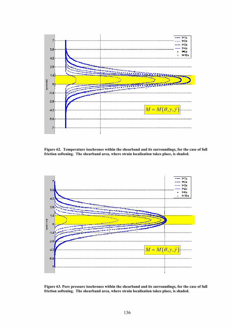
136

( ), ,M M θ γ γ=

Figure 62. Temperature isochrones within the shearband and its surroundings, for the case of full friction softening. The shearband area, where strain localisation takes place, is shaded.

( ), ,M M θ γ γ=

Figure 63. Pore pressure isochrones within the shearband and its surroundings, for the case of full friction softening. The shearband area, where strain localisation takes place, is shaded.

137

0 1 2 3 4 5 6 7 8 9 100

5

10

15

20

25

30landslide velocity

time (s)

velo

city

vd (m

/s)

Figure 64. slide velocity profile for the case of full friction softening.

0 1 2 3 4 5 6 7 8 9 100

20

40

60

80

100

120landslide displacement

time (s)

disp

lace

men

t xd (m

)

Figure 65. Slide displacement profile for the case of full friction softening.

138

5.5.7.4. Case of absent thermal friction softening

In order to assess the relative importance of the two main components of the FFS law

(thermal-dependence and strain-, strain rate- dependence) in the predicted values of

sliding velocity, it is now worth considering the case of absent thermal friction

softening (ATS), as proposed by Vardoulakis (2002a). This is easily achieved by setting

0g = in the friction-softening law (5.35). Results for temperature and pore pressure

isochrones are plotted in Figure 66 and Figure 67, velocity and displacement profiles

are plotted in Figure 68 and Figure 69.

By examining the graphs we cannot notice any appreciable difference with the case of

FFS. The calculated values for maximum temperature, pore pressure, slide velocity and

displacement are in fact smaller than those obtained for full softening by 0.5-1%, which

is negligible for our purposes. The comparison of results obtained for the three

examined friction-softening scenarios highlights the substantially more important role

played by strain- and strain rate-friction softening in determining the slide activation,

and is due to the specific form of the softening law (5.35): the decrease of M towards

the residual value according to the (twofold) hyperbolic law ( )ˆ ,M γ γ is so fast that no

perceptible difference is brought about by superimposing the linear decrease law

( )M θ .

( ),M M γ γ=

Figure 66. Temperature isochrones within the shearband and its surroundings, for the case of displacement and velocity softening only. The shearband area, where strain localisation takes place, is shaded.

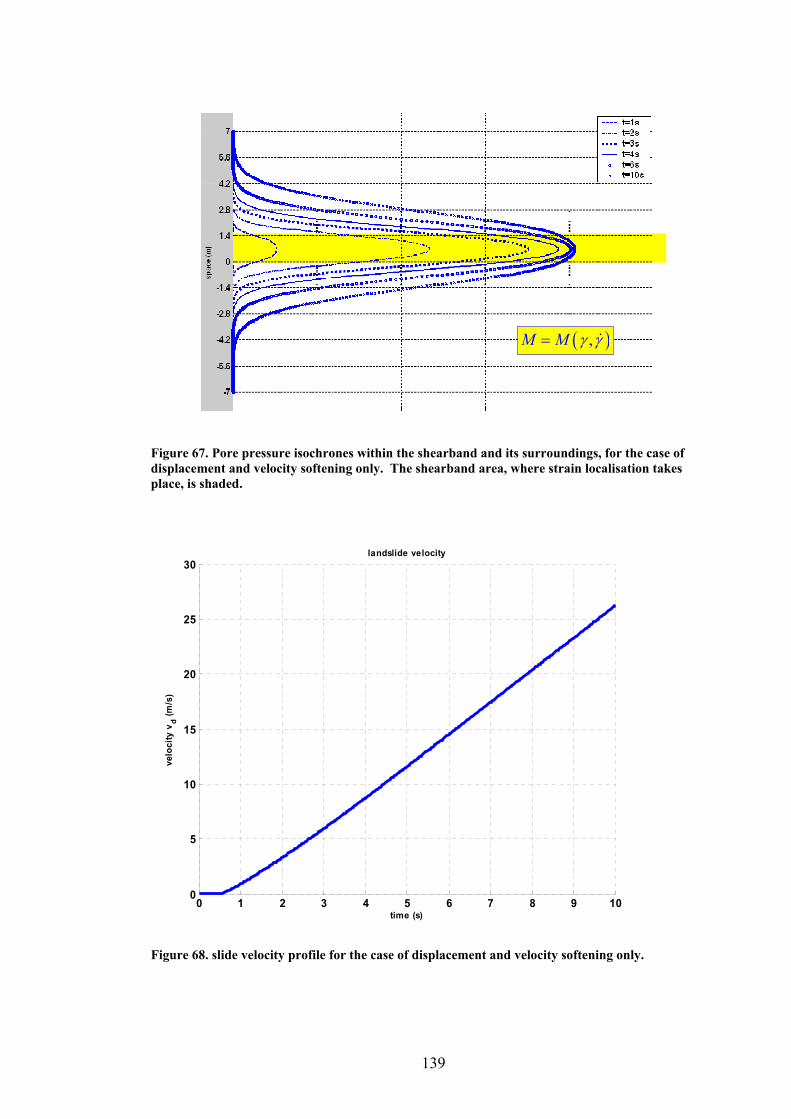
139

( ),M M γ γ=

Figure 67. Pore pressure isochrones within the shearband and its surroundings, for the case of displacement and velocity softening only. The shearband area, where strain localisation takes place, is shaded.

0 1 2 3 4 5 6 7 8 9 100

5

10

15

20

25

30landslide velocity

time (s)

velo

city

vd (m

/s)

Figure 68. slide velocity profile for the case of displacement and velocity softening only.

140

0 1 2 3 4 5 6 7 8 9 100

20

40

60

80

100

120landslide displacement

time (s)

disp

lace

men

t xd (m

)

Figure 69. Slide displacement profile for the case of displacement and velocity softening only.

5.5.7.5. Discussion on numerical results

All simulations reported in the last three sections predict a similar behaviour and

magnitude of results to those observed in Vajont, and are in accordance with those

calculated by the strain and strain-rate softening model of Vardoulakis (2002a). In

particular, a predicted final velocity of 20-25 m/s is in the bulk of the reported

observations for the Vajont slide (Hendron and Patton, 1985).

The TFS simulation shows that thermal-friction softening alone can indeed account for

catastrophic sliding, being potentially an important mechanism. Our choice for thermal

sensitivity of 210g −= proved to be reasonable, as it leads to realistic predictions and

matches with the available data on thermal-friction softening. On the other hand, the

simulations for the case of TFS should be only seen as an example to investigate the

impact of the newly introduced mechanism, since a realistic simulation must account for

the better established strain and strain-rate softening mechanisms. Such mechanisms

were included in the FFS and ATS simulations, which led to almost identical

predictions. By employing the hyperbolic strain- and strain rate-friction softening law

into the modified landslide model, slide activation for the Vajont case is anticipated to

0.5t ∼ seconds, and the influence of an additional thermal friction softening

141

mechanism is negligible. The outbreak of catastrophic acceleration in this case is

anticipated by some 1.5 seconds compared to Vardoulakis’ (2002a) calculations, as a

result of a quicker development of thermal pressurisation brought about by our

constitutive thermo-plastic modifications.

We may conclude that the numerical results presented give realistic predictions for the

final collapse phase of the Vajont case history, thus providing an essential validation

stage for our landslide model. On the other hand, it is worth recalling that the

intermittent, creep-like sliding phases of Vajont that preceded the catastrophic run-out

phase (cf. Section 2.1.4.2) cannot be reproduced by this model.

142

Chapter 6. Generalisation to infinite slope geometry

The results presented in Section 5.5.7 showed that the modified landslide model is

comprehensive and able to predict realistic values for the velocity of the Vajont slide.

The simulation of the Vajont case, which is the best documented catastrophic sliding

event in the literature, was a necessary validation step for the model, which can be now

employed to develop more general analyses.

The dynamical equation presented in Section 5.4 was derived from a friction circle

analysis, which presumes rotational failure for the sliding body and a constant average

vertical stress acting on the slip plane. Such assumptions were necessary to back-

analyse the Vajont case, known to have slid along an approximately circular rupture

surface. However, in order to provide a simple enough model that will allow us to

explore the impact of frictional heating and the role of different parameters, we will

now consider a more general geometry: the infinite slope.

6.1. Infinite slope analysis

The infinite slope or ‘block-on-slope’ idealisation consists of assuming the slope to be

uniform and of infinite extent (see e.g. Powrie, 1997). The slip plane is parallel to the

surface of the slope at a depth H. A unit length of slope is considered in the analysis,

and for a given geometry the gravity and seepage forces acting on it determine its safety

factor, if we are concerned about the stability of the slope (static analysis), or its

acceleration, if we are conducting a post-failure (dynamic) analysis. In Figure 70 the

infinite slope geometry is shown.

6.1.1. Static analysis to determine incipient failure conditions

The landslide model is dynamic and assumes ‘incipient failure’ as initial condition for

the mobilised strength. The limit equilibrium stress state, according to Coulomb’s law

τ μσ ′= is such that

,tan zx ultmob mob

zz

τμ φ

σ′= =

′ (6.1)

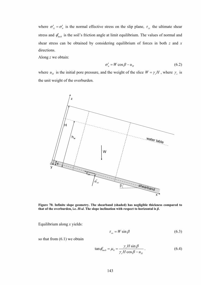
143

where zz nσ σ′ ′= is the normal effective stress on the slip plane, zxτ the ultimate shear

stress and mobφ′ is the soil’s friction angle at limit equilibrium. The values of normal and

shear stress can be obtained by considering equilibrium of forces in both z and x

directions.

Along z we obtain:

cosn HW uσ β′ = − (6.2)

where Hu is the initial pore pressure, and the weight of the slice sW Hγ= , where sγ is

the unit weight of the overburden.

W

τzx

H

d

z

β shearbandx

water tablehw

zzσ′

y

Figure 70. Infinite slope geometry. The shearband (shaded) has negligible thickness compared to that of the overburden, i.e. H»d. The slope inclination with respect to horizontal is β.

Equilibrium along x yields:

sinzx Wτ β= (6.3)

so that from (6.1) we obtain

0sintan

coss

mobs H

HH uγ βφ μ

γ β′ = =

−. (6.4)

144

The value of Hu depends on the groundwater conditions within the slope. As an

example, we will now consider the simple (although not most general, as we will

discuss in Section 7.3) case of groundwater flow parallel to the slope. In this case,

cosH w wu h γ β= (6.5)

where wγ is the unit weight of water and wh the height of the water table above the slip

plane. From (6.4) we may finally calculate the limit equilibrium friction angle as

arctan tansmob

s w w

HH hγφ β

γ γ⎛ ⎞

′ = ⎜ ⎟−⎝ ⎠. (6.6)

With such initial configuration, a small perturbation to equilibrium is needed to trigger

the movement of the slide. This can be done, for example, by reducing the obtained

value of mobφ′ by some 0.1% as it was done for the Vajont simulation (Section 5.5.6).

6.1.2. Dynamic analysis

The considered block is subjected after triggering to an acceleration driven by gravity.

The dynamic equation for the block along the x axis can be derived from Newton’s

second law of motion

xx

dvF mdt

= , (6.7)

where the mass of the 1-D block of Figure 70, knowing its volume ( )1 1 H= ⋅ ⋅ , the

overburden’s unit weight sγ and the acceleration of gravity g, is

sm Hgγ

= . (6.8)

From dynamic equilibrium, the force that applies in the direction of movement is the

result of the imbalance between the gravity component along x and the resisting force in

the slip plane due to friction and pore pressure:

( )sinx s zxF Hγ β τ= − (6.9)

where the shear stress zxτ , taken at mid-plane of the shearband where pressurisation is

expected to be maximum, is derived from Coulomb’s law. We may write

( ) ˆzx ntτ μσ ′= (6.10)

where ( )ˆ ˆ tμ μ= is the (potentially softening) friction coefficient (Section 5.2.1), and

( )n n tσ σ′ ′= the current normal effective stress which depends on the current values of

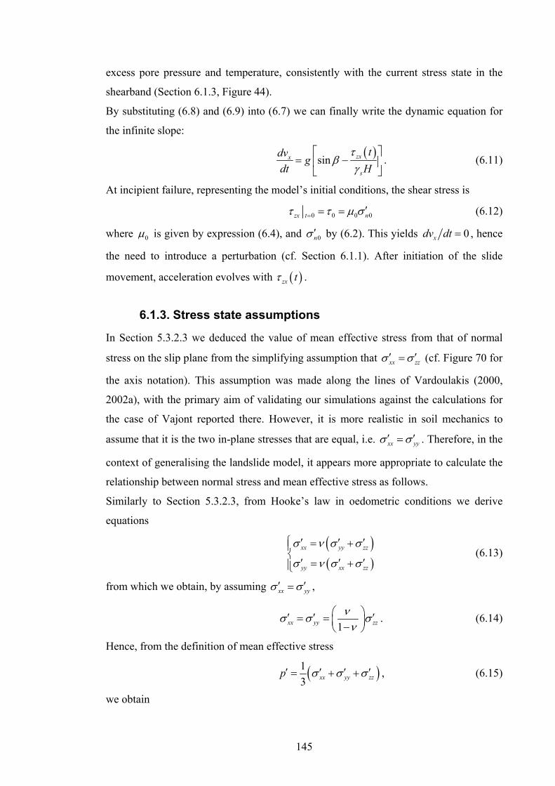
145

excess pore pressure and temperature, consistently with the current stress state in the

shearband (Section 6.1.3, Figure 44).

By substituting (6.8) and (6.9) into (6.7) we can finally write the dynamic equation for

the infinite slope:

( )sin zxx

s

tdv gdt H

τβ

γ⎡ ⎤

= −⎢ ⎥⎣ ⎦

. (6.11)

At incipient failure, representing the model’s initial conditions, the shear stress is

0 0 0 0zx t nτ τ μ σ= ′= = (6.12)

where 0μ is given by expression (6.4), and 0nσ ′ by (6.2). This yields 0xdv dt = , hence

the need to introduce a perturbation (cf. Section 6.1.1). After initiation of the slide

movement, acceleration evolves with ( )zx tτ .

6.1.3. Stress state assumptions

In Section 5.3.2.3 we deduced the value of mean effective stress from that of normal

stress on the slip plane from the simplifying assumption that xx zzσ σ′ ′= (cf. Figure 70 for

the axis notation). This assumption was made along the lines of Vardoulakis (2000,

2002a), with the primary aim of validating our simulations against the calculations for

the case of Vajont reported there. However, it is more realistic in soil mechanics to

assume that it is the two in-plane stresses that are equal, i.e. xx yyσ σ′ ′= . Therefore, in the

context of generalising the landslide model, it appears more appropriate to calculate the

relationship between normal stress and mean effective stress as follows.

Similarly to Section 5.3.2.3, from Hooke’s law in oedometric conditions we derive

equations

( )( )

xx yy zz

yy xx zz

σ ν σ σ

σ ν σ σ

⎧ ′ ′ ′= +⎪⎨

′ ′ ′= +⎪⎩ (6.13)

from which we obtain, by assuming xx yyσ σ′ ′= ,

1xx yy zzνσ σ σν

⎛ ⎞′ ′ ′= = ⎜ ⎟−⎝ ⎠. (6.14)

Hence, from the definition of mean effective stress

( )13 xx yy zzp σ σ σ′ ′ ′ ′= + + , (6.15)

we obtain

146

131zz n pνσ σ

ν−⎛ ⎞′ ′ ′= = ⎜ ⎟+⎝ ⎠

. (6.16)

From (6.16) we may calculate the current vertical effective stress acting on the

shearband from the current mean effective stress, given by expression (5.39).

Furthermore, we may calculate the initial mean effective stress from the initial normal

effective stress (6.2) as

0 01 13 1 np ν σ

ν+⎛ ⎞′ ′= ⎜ ⎟−⎝ ⎠

(6.17)

Following the same reasoning as in Section 5.3.2.3, from (6.17) we obtain a new

expression for the compressibility coefficient. The compressibility of the soil skeleton

from (5.94) becomes

1 13 1sk swc cν

ν+⎛ ⎞= ⎜ ⎟−⎝ ⎠

(6.18)

and (5.92) leads to the following expression for soil compressibility:

( )( )( )0

1

3 1 1wc nc

p e

κ ν

ν

+= +

′ − +. (6.19)

6.2. Numerical implementation

The infinite slope model contains the same heat and pore pressure equations as the

model of the rotational case (Chapter 5), and a new dynamical equation defined by

(6.11). To simulate the time evolution of temperature, excess pore pressure and slide

velocity it is then necessary to integrate numerically the following system:

( )2

2

2

2

(I)

(II)

ˆ(III) sin

di i

v m

b n

s

v tD F

t z du uct z t

dv gdt H

θ θ

θλ

μσβγ

⎧ ∂ ∂= +⎪

∂ ∂⎪⎪ ∂ ∂ ∂⎪ = +⎨ ∂ ∂ ∂⎪⎪ ⎡ ⎤′

= −⎪ ⎢ ⎥⎪ ⎣ ⎦⎩

(6.20)

Discretisation of governing equations (6.20) is done along the lines of Section 5.5.2.

Also in this case, the dynamical Equation (6.20)-(III) is a one-dimensional ODE,

describing the variation over time of the velocity of the block (hence the subscript b).

Similarly to Equation (5.115), the slide acceleration at the generic ith time-step is

expressed by function if :

147

( ) ( )ˆ , , ,

sini i i i i

b b ni

s

x v uf g

Hμ θ σ θ

βγ

⎡ ⎤′⎢ ⎥= −⎢ ⎥⎣ ⎦

. (6.21)

In the general case the stress depends on the current temperature and pore pressure at

the shearband mid-plane, and the friction coefficient depends on temperature, the

displacement and the velocity of the block. We can discretise the dynamical equation

with the 4th order Runge-Kutta approximation as:

1

1 2 11 2 16 3 6

n nn n nb bv v f f f

t

++ +−

= + +Δ

, (6.22)

and proceed to integration in the same way as detailed in Section 5.5.2. Given the

dependence on velocity of function (6.21), the discretised Runge-Kutta Equation (6.22)

cannot be solved directly for 1nbv + . The equation is therefore solved iteratively, using the

Ridders method to advance the solution (cf. Section 5.5.7.3).

The same considerations regarding the well-posedness of the heat equation hold for the

infinite slope model; carrying out the analysis of Section 5.5.4 shows that the infinite

slide model too remains well-posed for a very wide range of possible material values.

Also the stability analysis described in Section 5.5.5 is still relevant and valid for the

infinite slope model, as the heat and pore pressure equations remain unchanged

compared to the circular failure model of Chapter 5. This stability analysis is

implemented in our numerical code in order to automatically choose, before the start of

simulations, the computationally cheapest (i.e., the largest) time-step that complies with

condition (5.125).

6.3. Back-analysis of the Jiufengershan slide

The infinite slope model as presented above can now be applied to back-analyse other

case histories. The landslide of Jiufengershan (Section 2.1.4.5) appears to best suit the

purpose, because a) its planar geometry can be effectively represented by a block-on-

slope model, b) sufficient geomechanical data (although not as abundant as for the case

of Vajont) are available for a first-approximation simulation, and c) a pre-existing

dynamic numerical analisys (Chang et al., 2005a) provides us with some reference

values for a critical comparison.

148

6.3.1. Overview of the slide

The Jiufengershan landslide was triggered by the 1999 Chi-Chi earthquake in Taiwan. It

affected weathered rock and soil materials, which quickly slid along the bedding plane,

initially in a coherent manner and subsequently in a flow-like fashion (Chang et al.,

2005a), for a total of 1 km. The slip surface developed along a pre-existing bedding

fault, constituted of alternating beds of dark gray shale and muddy sandstone. Bedding-

parallel clay seams of 1-6 cm in thickness were found in the slip plane throughout the

slope, with clear slickensides and dip-slip striations (Wang et al., 2003).

The presence of frictionites in the slip plane of this slide (Section 2.3.1) proves the

occurrence of frictional heating which must have locally reached, in areas where direct

rock-to-rock contact was possible, temperatures in excess of 1000 °C (Chang et al.,

2005a). Moreover, the authors observe the possible occurrence of pore pressure build-

up when the permeability of the shear zone is low, as is the case for clay. Evidence of

pore water pressurisation in the shear zone was found through field observations, as

adjacent rock joints were found to be “filled with sheared mud injected from nearby

saturated clay layers that experienced fluidisation during the avalanche” (Chang et al.,

2005a).

Based on the above observations, Chang et al. (2005a) proposed a simple block-on-

slope thermo-mechanical model (cf. Section 2.3.2) which was employed to simulate the

landslide dynamics during the seismic triggering stage and the final collapse phase. The

authors proposed a back-calculation of the slide velocity and of temperature, pore

pressure and shear stress within the slip plane. These calculations show that the

catastrophic evolution of the slide (termed by the authors “avalanche regime”) can be

reproduced as soon as the thermal absorption coefficient, representing the fraction of

frictional energy that is transformed into heat, is above a threshold value. Nevertheless,

as pointed out in Section 2.3.2, the model equations of Chang et al. (2005a) do not seem

able to interpret in a physically well-based manner the landslide motion coupled with

the equations for heat flow and pore pressure diffusion across the shear zone, hence the

need for a more comprehensive understanding that the infinite slope model can provide.

6.3.2. Selection of parameters

The available data on the geometry and relevant geomechanical properties of the

Jiufengershan slide, reported by Chang et al. (2005a), Shou and Wang (2003) and Wang

et al. (2003), are reported in Table 5.

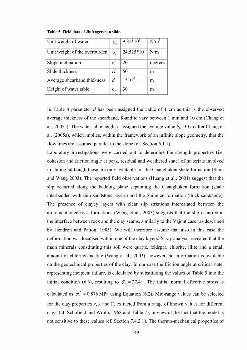
149

Table 5. Field data of Jiufengershan slide.

Unit weight of water wγ 9.81*103 N/m3

Unit weight of the overburden sγ 24.525*103 N/m3

Slope inclination β 20 degrees

Slide thickness H 50 m

Average shearband thickness d 1*10-2 m

Height of water table hw 30 m

In Table 4 parameter d has been assigned the value of 1 cm as this is the observed

average thickness of the shearband, found to vary between 1 mm and 10 cm (Chang et

al., 2005a). The water table height is assigned the average value hw=30 m after Chang et

al. (2005a), which implies, within the framework of an infinite slope geometry, that the

flow lines are assumed parallel to the slope (cf. Section 6.1.1).

Laboratory investigations were carried out to determine the strength properties (i.e.

cohesion and friction angle at peak, residual and weathered state) of materials involved

in sliding, although these are only available for the Changhuken shale formation (Shou

and Wang 2003). The reported field observations (Huang et al., 2001) suggest that the

slip occurred along the bedding plane separating the Changhuken formation (shale

interbedded with thin sandstone layers) and the Shihmen formation (thick sandstone).

The presence of clayey layers with clear slip striations intercalated between the

aforementioned rock formations (Wang et al., 2003) suggests that the slip occurred at

the interface between rock and the clay seams, similarly to the Vajont case (as described

by Hendron and Patton, 1985). We will therefore assume that also in this case the

deformation was localised within one of the clay layers. X-ray analysis revealed that the

main minerals constituting this soil were quartz, feldspar, chlorite, illite and a small

amount of chlorite/smectite (Wang et al., 2003); however, no information is available

on the geotechnical properties of the clay. In our case the friction angle at critical state,

representing incipient failure, is calculated by substituting the values of Table 5 into the

initial condition (6.6), resulting to 27.4csφ′ = ° . The initial normal effective stress is

calculated as 0.876nσ ′ = MPa using Equation (6.2). Mid-range values can be selected

for the clay properties κ, λ and Γ, extracted from a range of known values for different

clays (cf. Schofield and Wroth, 1968 and Table 7), in view of the fact that the model is

not sensitive to these values (cf. Section 7.4.2.1). The thermo-mechanical properties of

150

the soil, namely the thermo-elastic expansion coefficient sβ , the thermal diffusivity mk

and the thermal constant fC do not vary significantly for different types of soil (cf.

Alexandre et al., 1999, Vardoulakis, 2002a and Section 5.5.3.4). In the absence of better

data, they can be assigned the same values as for the Vajont case (Section 5.5.3). The

reference temperature θref can be set to 25°C to match the initial temperature in the

simulations of Chang et al. (2005a, Fig. 5), and appears reasonably higher than that of

Vajont considering the climatic differences between central Taiwan and the Alps.

In absence of direct measurements, the soil permeability can be set to an average value

representative of clayey soils, 1110wk −= m/s, which was adopted also in the case of

Vajont (Section 5.5.3). The thermal softening parameter γ, following the same reasoning

of Section 5.5.3.6 can be assigned the lower-mid-range value 210γ −= . Furthermore,

since no information is available on the friction-softening properties of the

Jiufengershan soil, parameters g , a1 and a2 (Section 5.2.1) are all set to zero for a first-

attempt simulation. The void ratio, isothermal preconsolidation stress and plastic

compressibility may be calculated as explained in Sections 5.5.3.1, 5.5.3.2 and 5.5.3.3

respectively. The above parameters are summarised in Table 6.

Table 6. Choice of parameters for Jiufengershan slide.

Slope of URL of clay κ 4.5*10-2 -----

Slope of NCL of clay λ 0.17 -----

Specific volume intercept of clay Γ 3.2 kPa

Soil (drained) Poisson’s ratio ν 0.3 -----

Compressibility of water cw 4.93*10-4 MPa-1

Reference temperature θref 25 °C

Soil thermal diffusivity coefficient km 1.45*10-7 m2/s

Thermo-elastic expansion coefficient sβ 7.41*10-5 °C-1

Thermal constant Cf 2.84 Mpa/°C

Soil permeability wk 10-11 m/s

Thermal softening parameter γ 10-2 -----

Calculated friction angle at CS csφ′ 27.4 degrees

Calculated initial normal effective stressnσ ′ 0.876 MPa

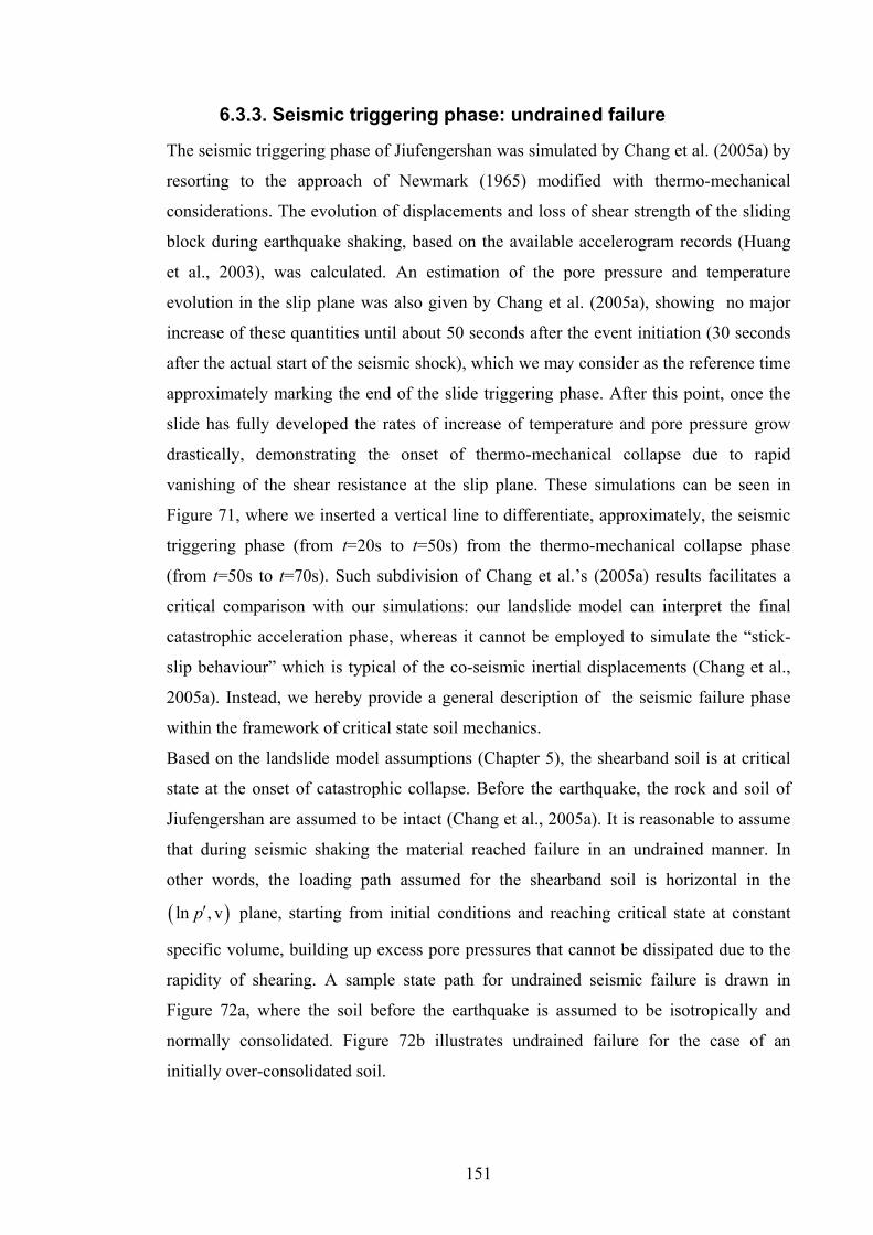
151

6.3.3. Seismic triggering phase: undrained failure

The seismic triggering phase of Jiufengershan was simulated by Chang et al. (2005a) by

resorting to the approach of Newmark (1965) modified with thermo-mechanical

considerations. The evolution of displacements and loss of shear strength of the sliding

block during earthquake shaking, based on the available accelerogram records (Huang

et al., 2003), was calculated. An estimation of the pore pressure and temperature

evolution in the slip plane was also given by Chang et al. (2005a), showing no major

increase of these quantities until about 50 seconds after the event initiation (30 seconds

after the actual start of the seismic shock), which we may consider as the reference time

approximately marking the end of the slide triggering phase. After this point, once the

slide has fully developed the rates of increase of temperature and pore pressure grow

drastically, demonstrating the onset of thermo-mechanical collapse due to rapid

vanishing of the shear resistance at the slip plane. These simulations can be seen in

Figure 71, where we inserted a vertical line to differentiate, approximately, the seismic

triggering phase (from t=20s to t=50s) from the thermo-mechanical collapse phase

(from t=50s to t=70s). Such subdivision of Chang et al.’s (2005a) results facilitates a

critical comparison with our simulations: our landslide model can interpret the final

catastrophic acceleration phase, whereas it cannot be employed to simulate the “stick-

slip behaviour” which is typical of the co-seismic inertial displacements (Chang et al.,

2005a). Instead, we hereby provide a general description of the seismic failure phase

within the framework of critical state soil mechanics.

Based on the landslide model assumptions (Chapter 5), the shearband soil is at critical

state at the onset of catastrophic collapse. Before the earthquake, the rock and soil of

Jiufengershan are assumed to be intact (Chang et al., 2005a). It is reasonable to assume

that during seismic shaking the material reached failure in an undrained manner. In

other words, the loading path assumed for the shearband soil is horizontal in the

( )ln , vp′ plane, starting from initial conditions and reaching critical state at constant

specific volume, building up excess pore pressures that cannot be dissipated due to the

rapidity of shearing. A sample state path for undrained seismic failure is drawn in

Figure 72a, where the soil before the earthquake is assumed to be isotropically and

normally consolidated. Figure 72b illustrates undrained failure for the case of an

initially over-consolidated soil.

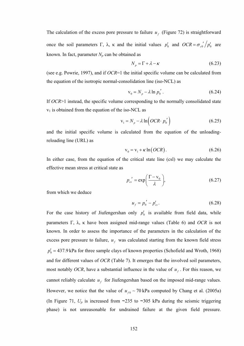
152

The calculation of the excess pore pressure to failure fu (Figure 72) is straightforward

once the soil parameters Γ, λ, κ and the initial values 0p′ and 0 0cOCR pσ ′ ′= are

known. In fact, parameter Np can be obtained as

pN λ κ= Γ + − (6.23)

(see e.g. Powrie, 1997), and if OCR=1 the initial specific volume can be calculated from

the equation of the isotropic normal-consolidation line (iso-NCL) as

0 0v lnpN pλ ′= − . (6.24)

If OCR>1 instead, the specific volume corresponding to the normally consolidated state

v1 is obtained from the equation of the iso-NCL as

( )1 0v lnpN OCR pλ ′= − ⋅ (6.25)

and the initial specific volume is calculated from the equation of the unloading-

reloading line (URL) as

( )0 1v v ln OCRκ= + . (6.26)

In either case, from the equation of the critical state line (csl) we may calculate the

effective mean stress at critical state as

0vexpcspλ

Γ −⎛ ⎞′ = ⎜ ⎟⎝ ⎠

, (6.27)

from which we deduce

0f csu p p′ ′= − . (6.28)

For the case history of Jiufengershan only 0p′ is available from field data, while

parameters Γ, λ, κ have been assigned mid-range values (Table 6) and OCR is not

known. In order to assess the importance of the parameters in the calculation of the

excess pore pressure to failure, fu was calculated starting from the known field stress

0 437.9p′ = kPa for three sample clays of known properties (Schofield and Wroth, 1968)

and for different values of OCR (Table 7). It emerges that the involved soil parameters,

most notably OCR, have a substantial influence in the value of fu . For this reason, we

cannot reliably calculate fu for Jiufengershan based on the imposed mid-range values.

However, we notice that the value of 0 70fu ∼ kPa computed by Chang et al. (2005a)

(In Figure 71, Up is increased from ~235 to ~305 kPa during the seismic triggering

phase) is not unreasonable for undrained failure at the given field pressure.

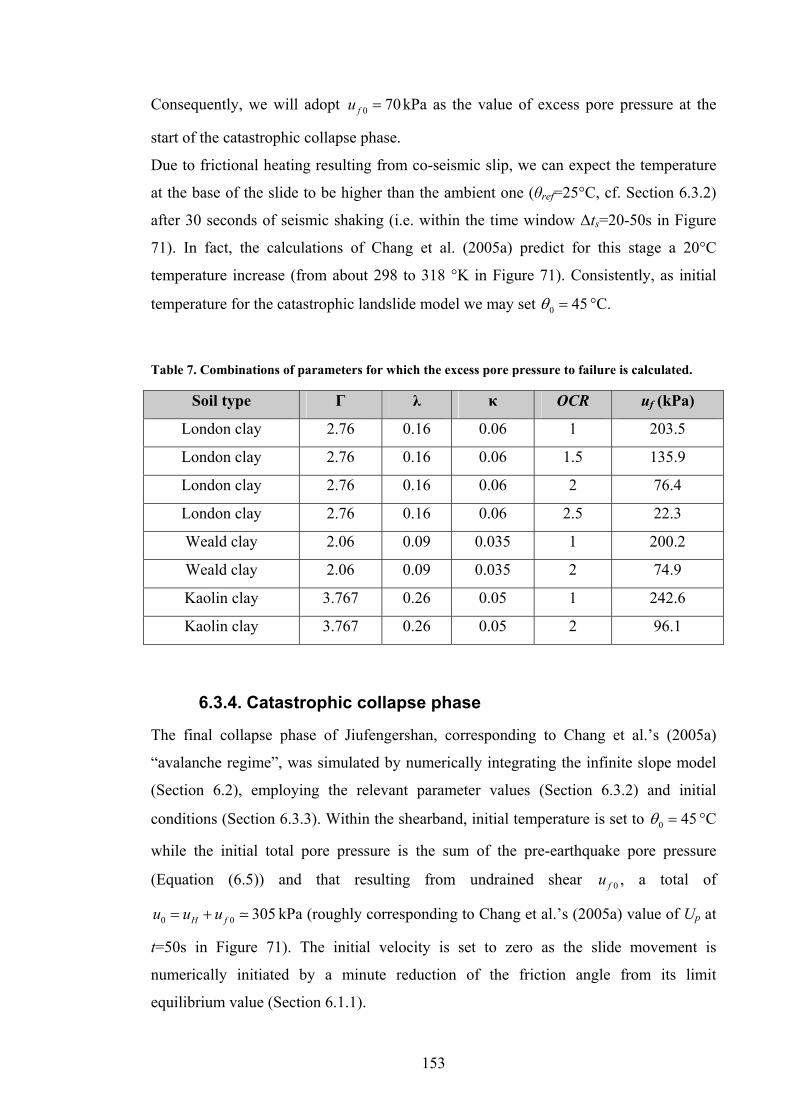
153

Consequently, we will adopt 0 70fu = kPa as the value of excess pore pressure at the

start of the catastrophic collapse phase.

Due to frictional heating resulting from co-seismic slip, we can expect the temperature

at the base of the slide to be higher than the ambient one (θref=25°C, cf. Section 6.3.2)

after 30 seconds of seismic shaking (i.e. within the time window Δts=20-50s in Figure

71). In fact, the calculations of Chang et al. (2005a) predict for this stage a 20°C

temperature increase (from about 298 to 318 °K in Figure 71). Consistently, as initial

temperature for the catastrophic landslide model we may set 0 45θ = °C.

Table 7. Combinations of parameters for which the excess pore pressure to failure is calculated.

Soil type Γ λ κ OCR uf (kPa)

London clay 2.76 0.16 0.06 1 203.5

London clay 2.76 0.16 0.06 1.5 135.9

London clay 2.76 0.16 0.06 2 76.4

London clay 2.76 0.16 0.06 2.5 22.3

Weald clay 2.06 0.09 0.035 1 200.2

Weald clay 2.06 0.09 0.035 2 74.9

Kaolin clay 3.767 0.26 0.05 1 242.6

Kaolin clay 3.767 0.26 0.05 2 96.1

6.3.4. Catastrophic collapse phase

The final collapse phase of Jiufengershan, corresponding to Chang et al.’s (2005a)

“avalanche regime”, was simulated by numerically integrating the infinite slope model

(Section 6.2), employing the relevant parameter values (Section 6.3.2) and initial

conditions (Section 6.3.3). Within the shearband, initial temperature is set to 0 45θ = °C

while the initial total pore pressure is the sum of the pre-earthquake pore pressure

(Equation (6.5)) and that resulting from undrained shear 0fu , a total of

0 0 305H fu u u= + kPa (roughly corresponding to Chang et al.’s (2005a) value of Up at

t=50s in Figure 71). The initial velocity is set to zero as the slide movement is

numerically initiated by a minute reduction of the friction angle from its limit

equilibrium value (Section 6.1.1).

154

Temperature and excess pore pressure were computed at each grid-point of the spatial

domain, and isochrones through the domain were produced at key time values, for a

time window of 20 seconds after initiation (Figure 73 and Figure 74). Compared to the

isochrones computed for Vajont (Figure 66 and Figure 67) where the initial normal

stress was higher (2.38 MPa vs 0.876 MPa of this case), the rate of production of both

temperature and pore pressure is here smaller: after 10s from initiation, at the shearband

mid-plane 55θ °C and 60u kPa. In both graphs, the flat profile of the isochrones

within the shearband for t=20s reveals the asymptotic convergence to a steady state for

heat production: temperature reaches the maximum value max 134θ °C as the

shearband soil liquefies due to full pressurisation and the shear stress tends to zero. This

is best illustrated in Figure 75, where the computed excess pore pressure and shear

stress at the shearband mid-plane are plotted against time: the weakening of shear

resistance is closely related to the raise of excess pore pressure, and the rates of both

functions tend to zero after t=18s.

Figure 71. From Chang et al. (2005a). Simulation of the time evolution of shear stress (τ), displacement (d), temperature (T) and pore pressure (Up) for the Jiufengershan slide in the catastrophic case scenario (avalanche regime). The seismic triggering phase, where the increase of pore pressure and temperature is not significant, lasts up to about 50 seconds, after which the drastic build-up of both T and Up determines catastrophic collapse due to rapid vanishing of the shear strength. The vertical dashed line marks the approximate boundary between the two phases.

155

ln(p’)

Iso-ncl

csl

λ λ

p’=1

Np

Γ

v

v1

p’=pcs’ p’=p0’ p’=σc0’

κ

v0

uf

IF

ln(p’)

Iso-ncl

csl

λ λ

p’=1

Np

Γ

v

v0

p’=pcs’ p’=p0=σc0’

uf

IF

(a) (b)S

peci

fic v

olum

e

Spe

cific

volu

me

Ln of mean effective stress Ln of mean effective stress

Figure 72. Sample stress paths of undrained failure from the initial undisturbed state (I) to the final critical state (F) in the compression plane, for the two cases of (a) initially NC soil and (b) initially OC soil.

In Figure 76 and Figure 77 the slide velocity and displacement are plotted against time.

After 10s from initiation, we obtain 0.9bv m/s and 1.6bx m, denoting a slower

acceleration in comparison to Vajont (Figure 68 and Figure 69). Nevertheless, the

reduction of shear strength is such that only 10 seconds later (at t=20s) also

Jiufengershan attains a velocity of 25 m/s, thus undergoing an equally catastrophic

evolution.

Field observations suggest that the maximum displacement of the Jiufengershan slide

was 1 km, and the maximum velocity reached was about 80 m/s, at a stage when the

mass could have lost its integrity and moved in a flow-like fashion (Chang et al.,

2005a). Nevertheless, this later-stage evolution appears to be well reproduced with the

infinite slope model: by extending our simulations to a time of 40 seconds after

initiation (Figure 78), we calculate a velocity of about 80 m/s after a displacement of

1000m.

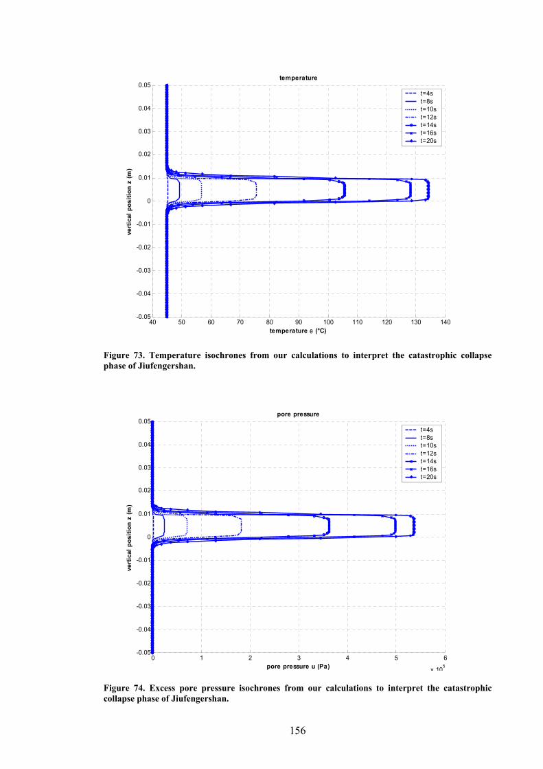
156

40 50 60 70 80 90 100 110 120 130 140-0.05

-0.04

-0.03

-0.02

-0.01

0

0.01

0.02

0.03

0.04

0.05temperature

vert

ical

pos

ition

z (m

)

temperature θ (°C)

t=4st=8st=10st=12st=14st=16st=20s

Figure 73. Temperature isochrones from our calculations to interpret the catastrophic collapse phase of Jiufengershan.

0 1 2 3 4 5 6

x 105

-0.05

-0.04

-0.03

-0.02

-0.01

0

0.01

0.02

0.03

0.04

0.05pore pressure

vert

ical

pos

ition

z (m

)

pore pressure u (Pa)

t=4st=8st=10st=12st=14st=16st=20s

Figure 74. Excess pore pressure isochrones from our calculations to interpret the catastrophic collapse phase of Jiufengershan.

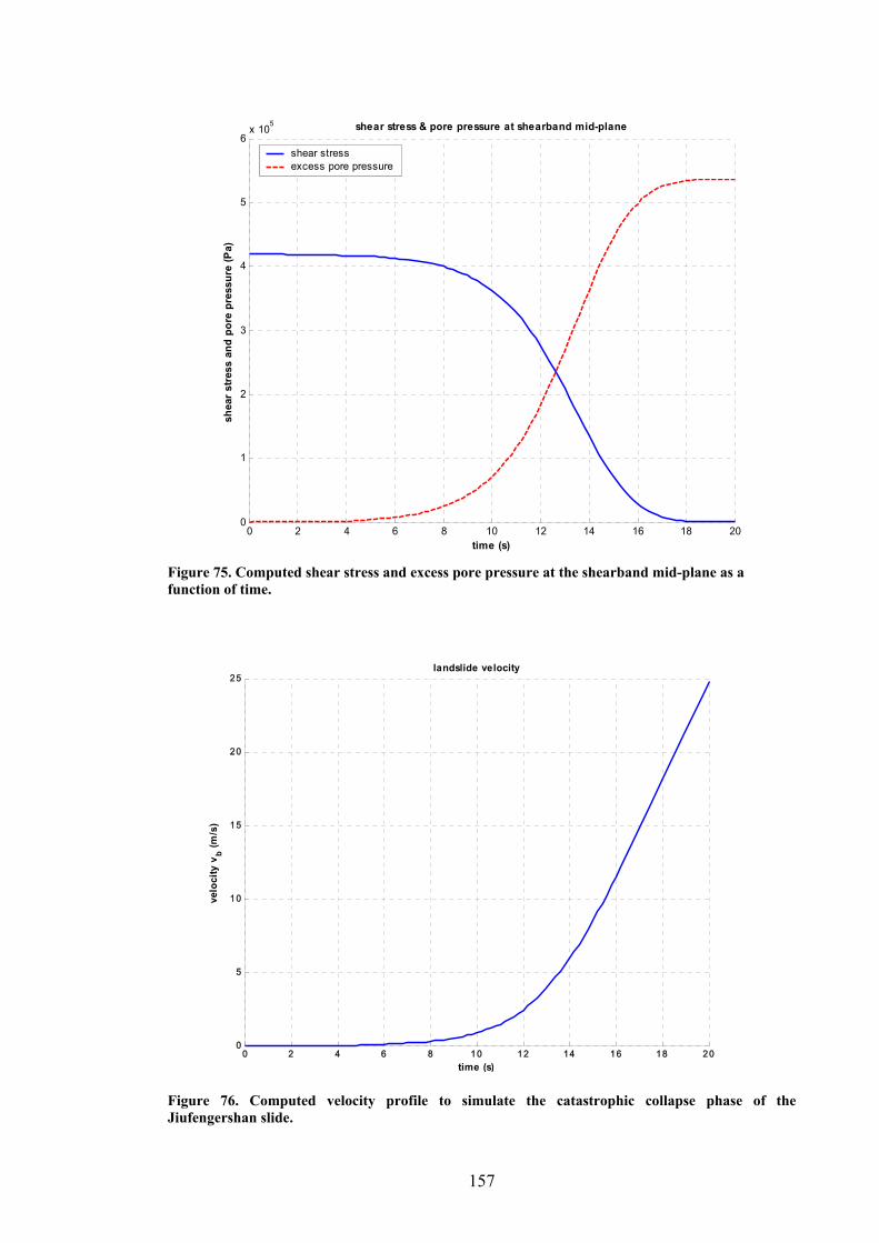
157

0 2 4 6 8 10 12 14 16 18 200

1

2

3

4

5

6x 105 shear stress & pore pressure at shearband mid-plane

time (s)

shea

r st

ress

and

por

e pr

essu

re (P

a)

shear stressexcess pore pressure

Figure 75. Computed shear stress and excess pore pressure at the shearband mid-plane as a function of time.

0 2 4 6 8 10 12 14 16 18 200

5

10

15

20

25landslide velocity

time (s)

velo

city

vb (m

/s)

Figure 76. Computed velocity profile to simulate the catastrophic collapse phase of the Jiufengershan slide.

158

0 2 4 6 8 10 12 14 16 18 200

20

40

60

80

100

120landslide displacement

time (s)

disp

lace

men

t xb (m

)

Figure 77. Computed displacement profile to simulate the catastrophic collapse phase of the Jiufengershan slide.

0 5 10 15 20 25 30 35 400

10

20

30

40

50

60

70

80

90

100landslide velocity and displacement

0 5 10 15 20 25 30 35 400

1000

2000

tim e (s )

disp

lace

men

t (m

)

velo

city

(m

/s)

velocity

displacement

Figure 78. Computed velocity and displacement of the Jiufengershan slide, plotted against time for the first 40 seconds of catastrophic collapse. The vertical dashed line marks the reaching of 1km of displacement, roughly corresponding to a velocity of 80 m/s.

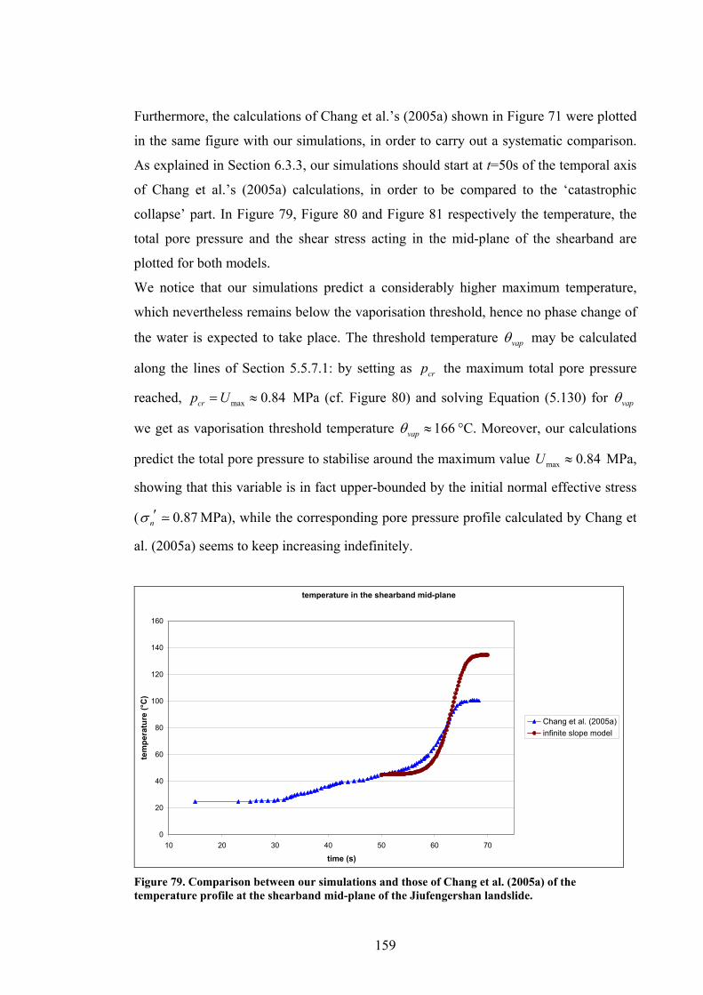
159

Furthermore, the calculations of Chang et al.’s (2005a) shown in Figure 71 were plotted

in the same figure with our simulations, in order to carry out a systematic comparison.

As explained in Section 6.3.3, our simulations should start at t=50s of the temporal axis

of Chang et al.’s (2005a) calculations, in order to be compared to the ‘catastrophic

collapse’ part. In Figure 79, Figure 80 and Figure 81 respectively the temperature, the

total pore pressure and the shear stress acting in the mid-plane of the shearband are

plotted for both models.

We notice that our simulations predict a considerably higher maximum temperature,

which nevertheless remains below the vaporisation threshold, hence no phase change of

the water is expected to take place. The threshold temperature vapθ may be calculated

along the lines of Section 5.5.7.1: by setting as crp the maximum total pore pressure

reached, max 0.84crp U= ≈ MPa (cf. Figure 80) and solving Equation (5.130) for vapθ

we get as vaporisation threshold temperature 166vapθ ≈ °C. Moreover, our calculations

predict the total pore pressure to stabilise around the maximum value max 0.84U ≈ MPa,

showing that this variable is in fact upper-bounded by the initial normal effective stress

( 0.87nσ ′ MPa), while the corresponding pore pressure profile calculated by Chang et

al. (2005a) seems to keep increasing indefinitely.

temperature in the shearband mid-plane

0

20

40

60

80

100

120

140

160

10 20 30 40 50 60 70

time (s)

tem

pera

ture

(°C

)

Chang et al. (2005a)infinite slope model

Figure 79. Comparison between our simulations and those of Chang et al. (2005a) of the temperature profile at the shearband mid-plane of the Jiufengershan landslide.

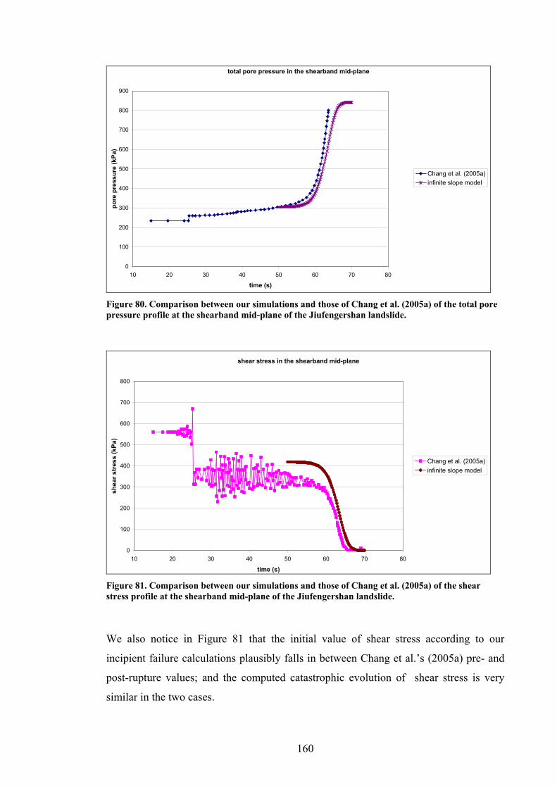
160

total pore pressure in the shearband mid-plane

0

100

200

300

400

500

600

700

800

900

10 20 30 40 50 60 70 80

time (s)

pore

pre

ssur

e (k

Pa)

Chang et al. (2005a)infinite slope model

Figure 80. Comparison between our simulations and those of Chang et al. (2005a) of the total pore pressure profile at the shearband mid-plane of the Jiufengershan landslide.

shear stress in the shearband mid-plane

0

100

200

300

400

500

600

700

800

10 20 30 40 50 60 70 80

time (s)

shea

r str

ess

(kPa

)

Chang et al. (2005a)infinite slope model

Figure 81. Comparison between our simulations and those of Chang et al. (2005a) of the shear stress profile at the shearband mid-plane of the Jiufengershan landslide.

We also notice in Figure 81 that the initial value of shear stress according to our

incipient failure calculations plausibly falls in between Chang et al.’s (2005a) pre- and

post-rupture values; and the computed catastrophic evolution of shear stress is very

similar in the two cases.

161

6.3.5. Cases of friction-softening soil and thinner shearband

As we will show in Section 7.4.2.1, the predictions of catastrophic collapse carried out

with our model are not substantially sensitive to the choice of standard soil parameters

such as Γ, λ, and κ. On the other hand, some parameters that are not always easy to

determine, like the shearband thickness d and the friction softening properties (static

and dynamic residual friction angles and rates of softening) may drastically affect the

predicted values. As an example, we will explore hereafter the effect of allowing for

friction-softening and that of assuming a thinner shearband in the Jiufengershan

simulations.

While the literature lacks information on typical values related to the dynamical

friction-softening of clays, some trends can be found on the static residual friction angle

(Section 2.1.4). For the Jiufengershan clay, we may assume that the latter is around 10°,

as is typical of soils with 50% clay fraction (Skempton, 1985). As an example, in our

simulation we will allow the friction angle to decrease with displacement only,

assuming for the rate of static softening, in the absence of better information, the same

value as for Vajont (cf. Section 5.2.1 and 5.5.3). By using for the other parameters the

same values as in Section 6.3.2, the simulations were run for a total time window of 20

seconds. The resulting temperature and pore pressure isochrones are shown in Figure 82

and Figure 83, and are similar to those in Section 6.3.4 (Figure 73 and Figure 74), but

the effect of the rapid decrease of friction with displacement is evident in the variable

slope of the shear stress plot (Figure 84): an initial, very steep branch due to friction

softening is followed by a relatively milder one, representing the continuation of the

shear resistance weakening due to pressurisation, towards the asymptotic attainment of

a liquefaction state, after t=12s. By comparing the shear stress and excess pore pressure

plots of Figure 84 to those in Figure 75 we notice that pressurisation is now more rapid,

due to more rapid frictional heating (Figure 85). In fact the rates of velocity and

displacement are heavily affected by material softening, as the slide reaches 500m at a

speed of almost 60 m/s after 20 seconds from initiation (Figure 86).

The effect of the shearband thickness on our calculations is shown by choosing for d the

lower-range value of 1mm (Chang et al., 2005a) whilst keeping all other parameters as

described in Section 6.3.2: more localised shearing causes (compared to the results in

Section 6.3.4) heating and pressurisation to be more concentrated around the shearband

mid-plane (Figure 87 and Figure 88). Also, thermal pressurisation is quicker, as in this

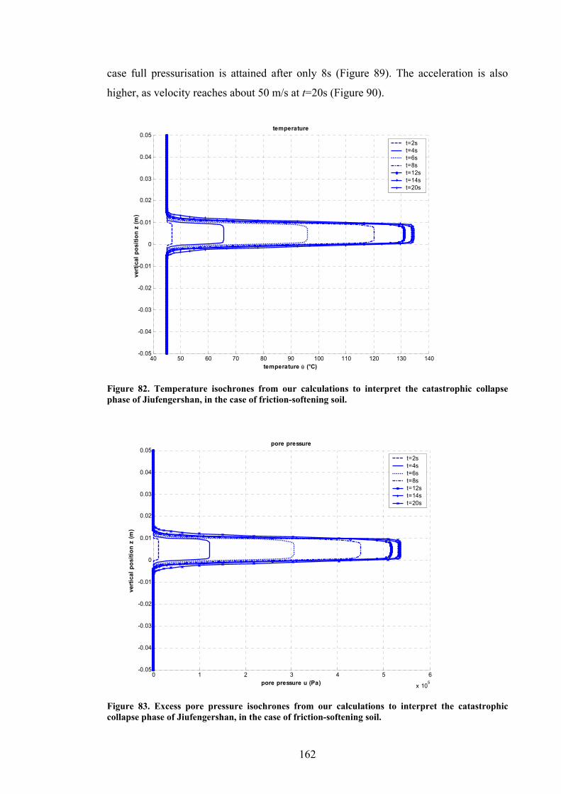
162

case full pressurisation is attained after only 8s (Figure 89). The acceleration is also

higher, as velocity reaches about 50 m/s at t=20s (Figure 90).

40 50 60 70 80 90 100 110 120 130 140-0.05

-0.04

-0.03

-0.02

-0.01

0

0.01

0.02

0.03

0.04

0.05temperature

verti

cal p

ositi

on z

(m)

temperature θ (°C)

t=2st=4st=6st=8st=12st=14st=20s

Figure 82. Temperature isochrones from our calculations to interpret the catastrophic collapse phase of Jiufengershan, in the case of friction-softening soil.

0 1 2 3 4 5 6

x 105

-0.05

-0.04

-0.03

-0.02

-0.01

0

0.01

0.02

0.03

0.04

0.05pore pressure

verti

cal p

ositi

on z

(m)

pore pressure u (Pa)

t=2st=4st=6st=8st=12st=14st=20s

Figure 83. Excess pore pressure isochrones from our calculations to interpret the catastrophic collapse phase of Jiufengershan, in the case of friction-softening soil.

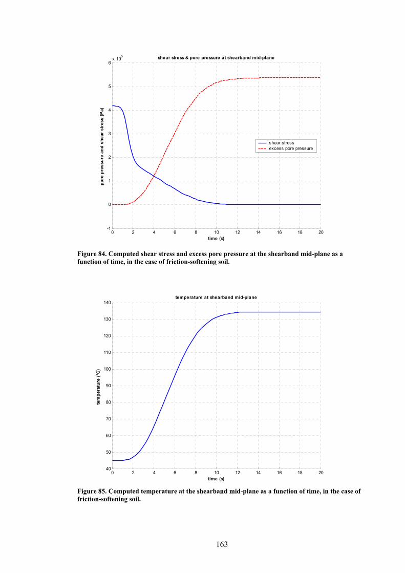
163

0 2 4 6 8 10 12 14 16 18 20-1

0

1

2

3

4

5

6x 105 shear stress & pore pressure at shearband mid-plane

time (s)

pore

pre

ssur

e an

d sh

ear

stre

ss (P

a)

shear stressexcess pore pressure

Figure 84. Computed shear stress and excess pore pressure at the shearband mid-plane as a function of time, in the case of friction-softening soil.

0 2 4 6 8 10 12 14 16 18 2040

50

60

70

80

90

100

110

120

130

140temperature at shearband mid-plane

time (s)

tem

pera

ture

(°C

)

Figure 85. Computed temperature at the shearband mid-plane as a function of time, in the case of friction-softening soil.

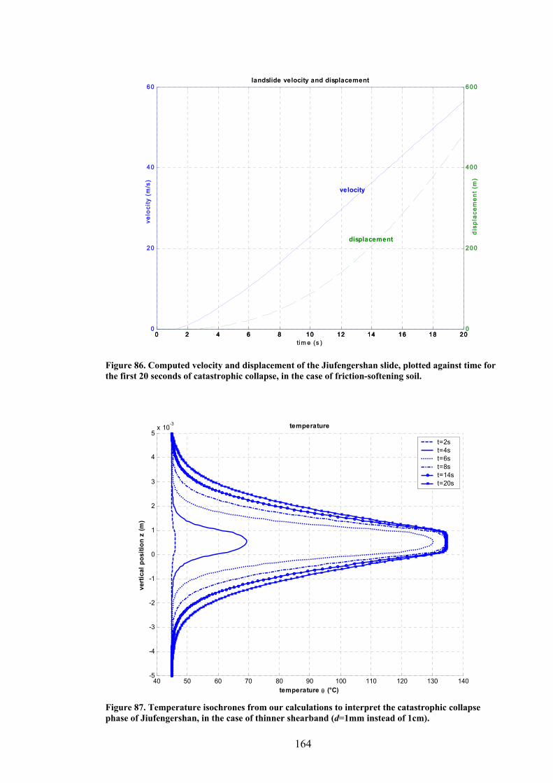
164

0 2 4 6 8 10 12 14 16 18 200

20

40

60landslide velocity and displacement

0 2 4 6 8 10 12 14 16 18 200

200

400

600

tim e (s )

velocity

displacement

velo

city

(m

/s)

dis

pla

cem

ent

(m

)

Figure 86. Computed velocity and displacement of the Jiufengershan slide, plotted against time for the first 20 seconds of catastrophic collapse, in the case of friction-softening soil.

40 50 60 70 80 90 100 110 120 130 140-5

-4

-3

-2

-1

0

1

2

3

4

5x 10

-3 temperature

verti

cal p

ositi

on z

(m)

temperature θ (°C)

t=2st=4st=6st=8st=14st=20s

Figure 87. Temperature isochrones from our calculations to interpret the catastrophic collapse phase of Jiufengershan, in the case of thinner shearband (d=1mm instead of 1cm).

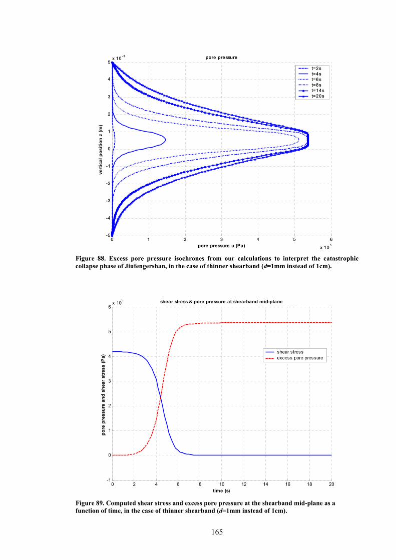
165

0 1 2 3 4 5 6

x 10 5

-5

-4

-3

-2

-1

0

1

2

3

4

5x 10 - 3 pore pressure

verti

cal p

ositi

on z

(m)

pore pressure u (Pa)

t=2st=4st=6st=8st=14st=20s

Figure 88. Excess pore pressure isochrones from our calculations to interpret the catastrophic collapse phase of Jiufengershan, in the case of thinner shearband (d=1mm instead of 1cm).

0 2 4 6 8 10 12 14 16 18 20-1

0

1

2

3

4

5

6x 10

5 shear stress & pore pressure at shearband mid-plane

time (s)

pore

pre

ssur

e an

d sh

ear

stre

ss (P

a)

shear stressexcess pore pressure

Figure 89. Computed shear stress and excess pore pressure at the shearband mid-plane as a function of time, in the case of thinner shearband (d=1mm instead of 1cm).

166

0 2 4 6 8 10 12 14 16 18 200

10

20

30

40

50

60landslide velocity

time (s)

velo

city

vd (m

/s)

Figure 90. Computed velocity profile to simulate the catastrophic collapse phase of the Jiufengershan slide, in the case of thinner shearband (d=1mm instead of 1cm).

167

Chapter 7. Parametric analysis to determine the critical conditions to catastrophic failure

After validating the infinite slope model with the back-analysis of the Jiufengershan

case history (Chapter 6), we may employ it to carry out a more general dynamic

analysis, with the aim of identifying the most important parameters that make a slope

prone to catastrophic failure. This is done by carrying out a number of simulations using

the landslide model while independently varying each relevant geometrical and

geomechanical property of the slide within a realistic range. Exploring all significant

combinations of parameters will allow us to determine the ones which maximise the

predicted slide velocity, i.e. those exacerbating the catastrophic character of the slide.

7.1. On the definition of ‘catastrophic’ slide

It has been shown in Chapter 6 that the infinite slope model is able to interpret the

dynamics of the final collapse phase of a landslide by calculating, among other relevant

quantities, the time evolution of the slide velocity. The velocity that a slide can reach is

indeed one of the key attributes to determine its destructive potential or, in other words,

to define how catastrophic a slide can be. Of particular interest to civil protection issues

is the slide acceleration, as predicting it can be critical to planning evacuation measures.

However, as discussed in Section 2.1.2, there cannot be a unique definition of

‘catastrophic’ slide, due to the wide variety of contexts in which landslides occur.

A criterion enabling us to formally discern between dangerous and non-dangerous cases

could still be established, based on the velocity reached by a slide after a certain

distance. For example, we could consider catastrophic any landslide that after 10 metres

of displacement reaches a velocity of 3 m/min (i.e., 0.05 m/s) or more. The latter value

constitutes the threshold velocity for ‘very rapid’ slides in the IUGS velocity

classification (Table 2); while 10 metres can arguably be considered, in first

approximation, a distance large enough for a slide to be noticed, and maybe small

enough to avoid major damage. Such a criterion can be useful when a potentially

unstable slope is considered and, all relevant field data being available, a prediction of

the dynamic evolution of the slide is attempted. On the other hand, our main aim is to

establish a general rule, enabling us to identify the most important properties that make

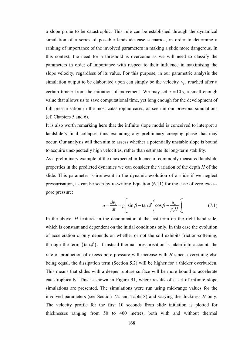
168

a slope prone to be catastrophic. This rule can be established through the dynamical

simulation of a series of possible landslide case scenarios, in order to determine a

ranking of importance of the involved parameters in making a slide more dangerous. In

this context, the need for a threshold is overcome as we will need to classify the

parameters in order of importance with respect to their influence in maximising the

slope velocity, regardless of its value. For this purpose, in our parametric analysis the

simulation output to be elaborated upon can simply be the velocity vτ , reached after a

certain time τ from the initiation of movement. We may set 10τ = s, a small enough

value that allows us to save computational time, yet long enough for the development of

full pressurisation in the most catastrophic cases, as seen in our previous simulations

(cf. Chapters 5 and 6).

It is also worth remarking here that the infinite slope model is conceived to interpret a

landslide’s final collapse, thus excluding any preliminary creeping phase that may

occur. Our analysis will then aim to assess whether a potentially unstable slope is bound

to acquire unexpectedly high velocities, rather than estimate its long-term stability.

As a preliminary example of the unexpected influence of commonly measured landslide

properties in the predicted dynamics we can consider the variation of the depth H of the

slide. This parameter is irrelevant in the dynamic evolution of a slide if we neglect

pressurisation, as can be seen by re-writing Equation (6.11) for the case of zero excess

pore pressure:

sin tan cosx H

s

dv ua gdt H

β φ βγ

⎡ ⎤⎛ ⎞′= = − −⎢ ⎥⎜ ⎟⎝ ⎠⎣ ⎦

(7.1)

In the above, H features in the denominator of the last term on the right hand side,

which is constant and dependent on the initial conditions only. In this case the evolution

of acceleration a only depends on whether or not the soil exhibits friction-softening,

through the term ( )tanφ′ . If instead thermal pressurisation is taken into account, the

rate of production of excess pore pressure will increase with H since, everything else

being equal, the dissipation term (Section 5.2) will be higher for a thicker overburden.

This means that slides with a deeper rupture surface will be more bound to accelerate

catastrophically. This is shown in Figure 91, where results of a set of infinite slope

simulations are presented. The simulations were run using mid-range values for the

involved parameters (see Section 7.2 and Table 8) and varying the thickness H only.

The velocity profile for the first 10 seconds from slide initiation is plotted for

thicknesses ranging from 50 to 400 metres, both with and without thermal

169

pressurisation. Calculations relative to the latter case all lead to the same prediction,

represented by the thin dashed line at the bottom of the plot. The velocity reached after

10s in this case is of the order of metres/hour, while if thermo-mechanical effects are

taken into account the velocity after 10s increases with H by several orders of

magnitude, up to 10 m/s in the extreme case of H=400m.

The above example highlights the need for a systematic study, since in the framework

of the thermo-mechanical infinite slope model other parameters might be unexpectedly

important in the catastrophic evolution of a slide. The parameteric analysis is presented

hereafter.

0 1 2 3 4 5 6 7 8 9 10

0

1

2

3

4

5

6

7

8

9

10landslide velocity

time (s)

velo

city

vd (m

/s)

h=50mh=100mh=200mh=300mh=400mh=50-400m, no pressurisation

Figure 91. Preliminary study on the effect of the overburden thickness H on the slide velocity.

7.2. Choice of parameters and their range

7.2.1. Selected parameters

The main parameters involved in the dynamic analysis of a landslide are listed in

Section 6.3.2. Of these, the properties that are bound to exhibit more variability for

different landslide cases will be chosen hereafter as parameters for our study. A set of

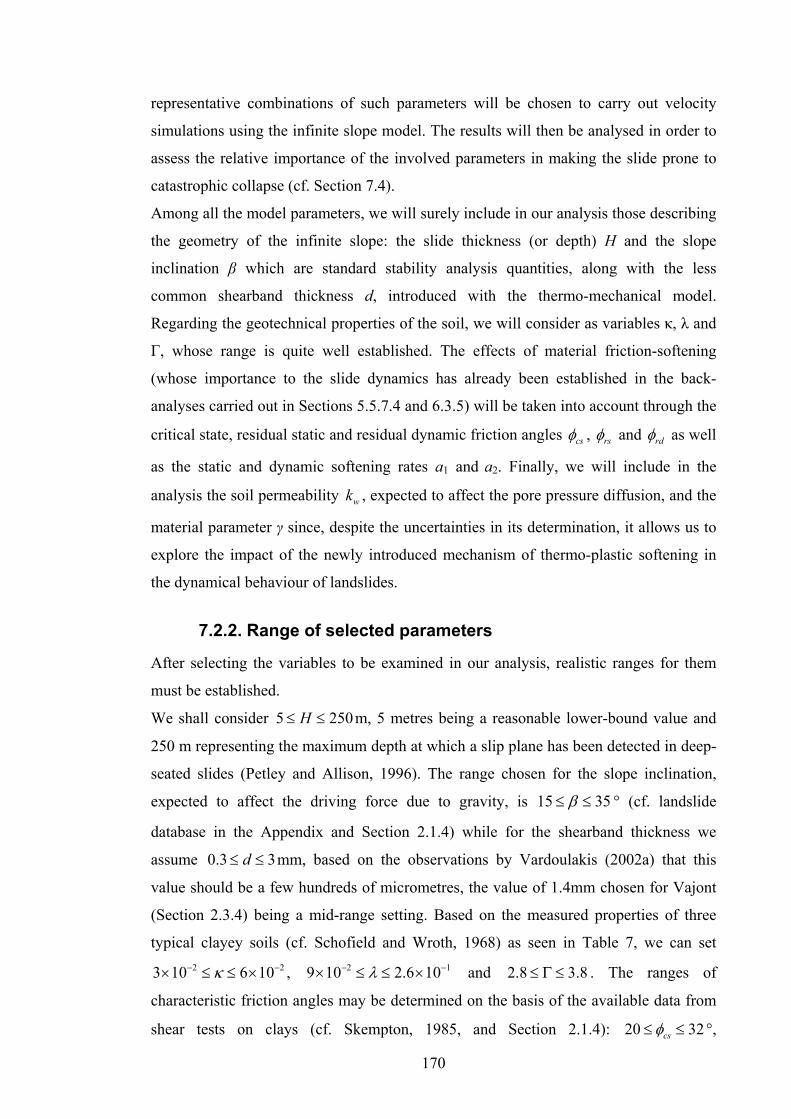
170

representative combinations of such parameters will be chosen to carry out velocity

simulations using the infinite slope model. The results will then be analysed in order to

assess the relative importance of the involved parameters in making the slide prone to

catastrophic collapse (cf. Section 7.4).

Among all the model parameters, we will surely include in our analysis those describing

the geometry of the infinite slope: the slide thickness (or depth) H and the slope

inclination β which are standard stability analysis quantities, along with the less

common shearband thickness d, introduced with the thermo-mechanical model.

Regarding the geotechnical properties of the soil, we will consider as variables κ, λ and

Γ, whose range is quite well established. The effects of material friction-softening

(whose importance to the slide dynamics has already been established in the back-

analyses carried out in Sections 5.5.7.4 and 6.3.5) will be taken into account through the

critical state, residual static and residual dynamic friction angles csφ , rsφ and rdφ as well

as the static and dynamic softening rates a1 and a2. Finally, we will include in the

analysis the soil permeability wk , expected to affect the pore pressure diffusion, and the

material parameter γ since, despite the uncertainties in its determination, it allows us to

explore the impact of the newly introduced mechanism of thermo-plastic softening in

the dynamical behaviour of landslides.

7.2.2. Range of selected parameters

After selecting the variables to be examined in our analysis, realistic ranges for them

must be established.

We shall consider 5 250H≤ ≤ m, 5 metres being a reasonable lower-bound value and

250 m representing the maximum depth at which a slip plane has been detected in deep-

seated slides (Petley and Allison, 1996). The range chosen for the slope inclination,

expected to affect the driving force due to gravity, is 15 35β≤ ≤ ° (cf. landslide

database in the Appendix and Section 2.1.4) while for the shearband thickness we

assume 0.3 3d≤ ≤ mm, based on the observations by Vardoulakis (2002a) that this

value should be a few hundreds of micrometres, the value of 1.4mm chosen for Vajont

(Section 2.3.4) being a mid-range setting. Based on the measured properties of three

typical clayey soils (cf. Schofield and Wroth, 1968) as seen in Table 7, we can set 2 23 10 6 10κ− −× ≤ ≤ × , 2 19 10 2.6 10λ− −× ≤ ≤ × and 2.8 3.8≤ Γ ≤ . The ranges of

characteristic friction angles may be determined on the basis of the available data from

shear tests on clays (cf. Skempton, 1985, and Section 2.1.4): 20 32csφ≤ ≤ °,

171

10 20rsφ≤ ≤ ° and 4 10rdφ≤ ≤ °. The rates of friction-softening, on the other hand, have

hardly ever been estimated in the literature, hence we will select for both a1 and a2 a

broad range, representing all possible scenarios spanning from the extremely slow to the

very sudden softening case: 5 3110 10a− ≤ ≤ , 5 3

210 10a− ≤ ≤ . From the few available data

on the friction-softening behaviour of clays (Skempton, 1985, Lehane and Jardine, 1992

and Tikka and Hutchinson, 1999) we may deduce that a reasonable mid-range value for

both a1 and a2 is 0.1, as proposed by Vardoulakis (2002a) for the Vajont clay.

Permeability is assumed to vary as 13 610 10wk− −≤ ≤ m/s, the upper-bound value

representing fissured clays (cf. Powrie, 1997) and the lower-bound one representing a

uniform clay whose permeability has decreased due to prolonged shearing and

consequent alignment of the platy particles parallel to the direction of motion

(Vardoulakis, 2000). The range chosen for the parameter γ of the thermoplastic model is 3 110 10γ− −≤ ≤ , in agreement with the range experimentally observed whilst ensuring

the calculation of realistic values for the pressurisation coefficient (cf. Section 5.5.3.6).

7.2.3. Parameters that are kept constant

The parameters involved in the landslide model (Section 6.3.2) that do not exhibit in

nature a high variability, or that are not expected to influence the results with their

variation will be kept constant in our parametric analysis. In particular, the soil thermal

properties sβ , mk and fC are assigned a mean value which is typical of clays (Section

6.3.2), the Poisson’s ratio ν is set equal to the mean value 0.3 and the rate of thermal-

friction softening g is set to zero, due to the lack of information on this phenomenon

and to its ascertained secondary importance to static and dynamic material friction

softening (Section 5.5.7.4). The reference temperature θref can be set to 20°C,

representing a mean value between the initial temperature of the Vajont simulation and

that of the Jiufengershan simulation. The compressibility of water cw, the unit weight of

water γw and the unit weight of the overburden γs are assigned the same values as in

Section 6.3.2, which can be considered representative of average conditions.

7.3. Generalisation of initial conditions

The static analysis leading to the determination of incipient failure conditions for the

infinite slope as presented in Section 6.1.1 is appropriate for the back-analysis of

Jiufengershan, but lacks generality as far as the assumed groundwater conditions are

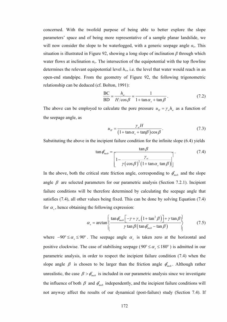
172

concerned. With the twofold purpose of being able to better explore the slope

parameters’ space and of being more representative of a sample planar landslide, we

will now consider the slope to be waterlogged, with a generic seepage angle αs. This

situation is illustrated in Figure 92, showing a long slope of inclination β through which

water flows at inclination αs. The intersection of the equipotential with the top flowline

determines the relevant equipotential level hw, i.e. the level that water would reach in an

open-end standpipe. From the geometry of Figure 92, the following trigonometric

relationship can be deduced (cf. Bolton, 1991):

BC 1BD cos 1 tan tan

w

s

hH β α β

= =+ +

. (7.2)

The above can be employed to calculate the pore pressure H w wu hγ= as a function of

the seepage angle, as

( )1 tan tan cos

wH

s

Hu γα β β

=+ +

. (7.3)

Substituting the above in the incipient failure condition for the infinite slope (6.4) yields

( ) ( )2

tantan

1cos 1 tan tan

mob

w

s

βφγ

γ β α β

′ =⎡ ⎤−⎢ ⎥

+⎢ ⎥⎣ ⎦

. (7.4)

In the above, both the critical state friction angle, corresponding to mobφ′ and the slope

angle β are selected parameters for our parametric analysis (Section 7.2.1). Incipient

failure conditions will be therefore determined by calculating the seepage angle that

satisfies (7.4), all other values being fixed. This can be done by solving Equation (7.4)

for sα , hence obtaining the following expression:

( )

( )

2tan 1 tan tanarctan

tan tan tanmob w

smob

φ γ γ β γ βα

γ β φ β

⎧ ⎫⎡ ⎤′ − + + +⎪ ⎪⎣ ⎦= ⎨ ⎬′ −⎪ ⎪⎩ ⎭ (7.5)

where 90 90sα− ° ≤ ≤ ° . The seepage angle sα is taken zero at the horizontal and

positive clockwise. The case of stabilising seepage (90 180sα° ≤ ≤ ° ) is admitted in our

parametric analysis, in order to respect the incipient failure condition (7.4) when the

slope angle β is chosen to be larger than the friction angle mobφ′ . Although rather

unrealistic, the case mobβ φ′> is included in our parametric analysis since we investigate

the influence of both β and mobφ′ independently, and the incipient failure conditions will

not anyway affect the results of our dynamical (post-failure) study (Section 7.4). If

173

mobβ φ′> the resulting sα will be greater than 90°, however, due to the nature of

function arctangent, Equation (7.5) yields 0s negα α= < instead. This limitation is

overcome numerically by setting, whenever mobβ φ′> ,

s negα π α= + , (7.6)

which allows us to calculate the correct value of [ ]90 ,180sα ∈ ° ° .

d

z

β

x

H

β

αs

z

x

hw

A

B

C

D

Figure 92. Scheme of an infinite slope of inclination β through which water is flowing at inclination αs. An open-end standpipe is represented to highlight the equipotential level relevant to points situated along segment AB.

As discussed in Section 6.1.1, with the initial configuration described by Equation (6.4)

a perturbation of the incipient failure conditions is needed to trigger the movement of

the slide. This can be done by increasing by a small HuΔ the limit equilibrium value of

Hu , as obtained by substituting (7.5) into (7.3). For example, we may set

0.01HuΔ = Pa.

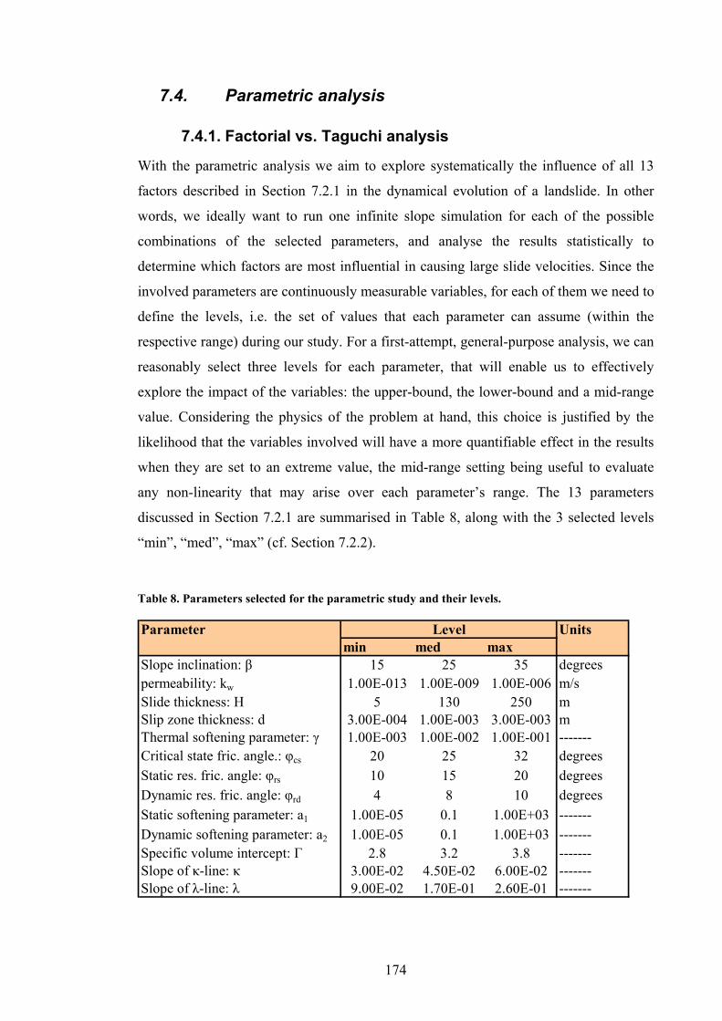
174

7.4. Parametric analysis

7.4.1. Factorial vs. Taguchi analysis

With the parametric analysis we aim to explore systematically the influence of all 13

factors described in Section 7.2.1 in the dynamical evolution of a landslide. In other

words, we ideally want to run one infinite slope simulation for each of the possible

combinations of the selected parameters, and analyse the results statistically to

determine which factors are most influential in causing large slide velocities. Since the

involved parameters are continuously measurable variables, for each of them we need to

define the levels, i.e. the set of values that each parameter can assume (within the

respective range) during our study. For a first-attempt, general-purpose analysis, we can

reasonably select three levels for each parameter, that will enable us to effectively

explore the impact of the variables: the upper-bound, the lower-bound and a mid-range

value. Considering the physics of the problem at hand, this choice is justified by the

likelihood that the variables involved will have a more quantifiable effect in the results

when they are set to an extreme value, the mid-range setting being useful to evaluate

any non-linearity that may arise over each parameter’s range. The 13 parameters

discussed in Section 7.2.1 are summarised in Table 8, along with the 3 selected levels

“min”, “med”, “max” (cf. Section 7.2.2).

Table 8. Parameters selected for the parametric study and their levels.

Parameter Unitsmin med max

Slope inclination: β 15 25 35 degreespermeability: kw 1.00E-013 1.00E-009 1.00E-006 m/sSlide thickness: H 5 130 250 mSlip zone thickness: d 3.00E-004 1.00E-003 3.00E-003 mThermal softening parameter: γ 1.00E-003 1.00E-002 1.00E-001 -------Critical state fric. angle.: φcs 20 25 32 degreesStatic res. fric. angle: φrs 10 15 20 degreesDynamic res. fric. angle: φrd 4 8 10 degreesStatic softening parameter: a1 1.00E-05 0.1 1.00E+03 -------Dynamic softening parameter: a2 1.00E-05 0.1 1.00E+03 -------Specific volume intercept: Γ 2.8 3.2 3.8 -------Slope of κ-line: κ 3.00E-02 4.50E-02 6.00E-02 -------Slope of λ-line: λ 9.00E-02 1.70E-01 2.60E-01 -------

Level

175

In order to design our parametric analysis we may resort to the concepts of

Experimental Design, a branch of Engineering Statistics that deals with deliberately

changing one or more variables in a process, in order to observe the effect that the

changes have on one or more response variables (e.g. see NIST/SEMATECH, 2003). In

our case, the process is the landslide simulation, the variables are the 13 selected

parameters, and the response variable is the calculated velocity after 10 seconds from

slide initiation.

Once the significant process variables have been selected together with the relevant

levels, the type of experimental design must be chosen, among the many available,

based on the objectives of the experiment and the number of factors to be investigated.

The most straightforward method is a design in which every setting of every factor

appears with every setting of every other factor, called the full factorial method. This

implies running an experiment (i.e. a simulation) for each of the possible combinations

of parameters. The number of needed experiments in this case is pN , where N is the

number of levels chosen for each variable and p the number of variables. With the

settings of Table 8, the number of simulations that we need for a full factorial analysis is

then 133 1,594,323= . Considering that the computational time for a 10-seconds

simulation with our infinite slope numerical code varies between 1 minute and 1 week,

depending on the resulting time-step from the stability analysis (in turn depending on

the value of key parameters such as the permeability kw and the shearband thickness d,

cf. Section 5.5.5), a full factorial analysis is impractical.

Several other methods are available in the literature, notably the ‘randomised’ and the

‘fractional factorial’ designs (e.g. see NIST/SEMATECH, 2003), involving a reduction

of the needed number of experiments compared to a full factorial analysis. While the

randomised design, if applied to our case, may lead to an incorrect interpretation of the

physical phenomena involved, a fractional factorial analysis would be extremely

complicated from the point of view of statistical design, whilst not necessarily allowing

us to save much computational time.

The method that was found to best suit our purposes due to its robustness, flexibility

and simplicity, is the renowned Taguchi method (e.g., Taguchi et al., 1989, Peace,

1993). The experimental strategy within the framework of Taguchi is based on

orthogonal arrays (Section 7.4.2), defining the number of experiments needed to explore

all statistically significant parameters’ combinations. With our settings of 13 parameters

and 3 levels (Table 8), a Taguchi analysis will need only 27 simulations to be

176

completed, to which some basic statistical analysis of results will have to follow. The

practicality of this method is apparent, also considering that it is possible to perform

verification runs (see Section 7.4.2.2) to double-check the reliability of the analysis’

results. We elaborate on the Taguchi method in the next section.

7.4.2. A general Taguchi analysis

The theory of the Taguchi experimental design will be illustrated hereafter, alongside its

application to the infinite slope parametric analysis outlined in Table 8.

A fundamental step in the design of our analysis is the definition of a suitable

orthogonal array, i.e., a 2-dimensional matrix defining the variables’ settings for each of

the experiments needed. Each row of the matrix contains the list of settings for all

parameters in one experiment. Each column corresponds to one of the variables, and

contains all the values that this variable will be assigned during the experiments. As an

example a generic orthogonal array for a 3-variable, 2-level analysis is reported in Table

9, where α, β and γ indicate the variables, the H’s and L’s the two levels decided for

each parameter (e.g. a ‘high’ and ‘low’ value within a range) and the numbers on the

leftmost column denote the number of experimental runs (or equivalently, the number

of combinations of factors). We observe that in this sample scenario only 4 runs are

needed to explore the significant combinations of 3 parameters with two levels, instead

of the 23=8 runs needed in a full factorial analysis.

Table 9. Sample orthogonal array containing the settings for a 3-parameter, 2-level analysis.

Experiment n.\ parameter α β γ1 L α L β L γ

2 L α H β H γ

3 H α L β H γ

4 H α H β L γ

Orthogonal arrays must respond to specific requirements, and they cannot be created

with any chosen combination of parameters and levels. The fundamental property of

these matrices is statistical independence (Peace, 1993): not only within each column is

present an equal number of occurrences for each level (e.g. in Table 9, in each column

both level H and level L appear twice), but also the columns are interrelated

(orthogonal) between one another; i.e. for each level within one column, each level

within any other column will occur an equal number of times as well. The latter

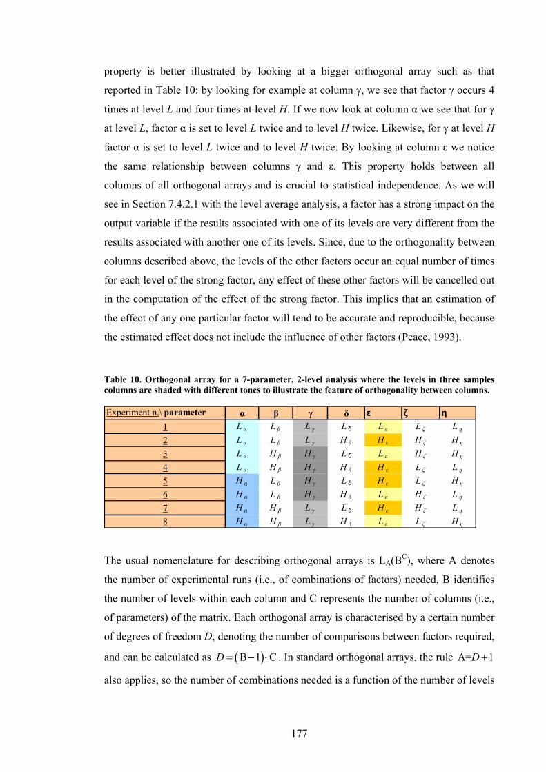
177

property is better illustrated by looking at a bigger orthogonal array such as that

reported in Table 10: by looking for example at column γ, we see that factor γ occurs 4

times at level L and four times at level H. If we now look at column α we see that for γ

at level L, factor α is set to level L twice and to level H twice. Likewise, for γ at level H

factor α is set to level L twice and to level H twice. By looking at column ε we notice

the same relationship between columns γ and ε. This property holds between all

columns of all orthogonal arrays and is crucial to statistical independence. As we will

see in Section 7.4.2.1 with the level average analysis, a factor has a strong impact on the

output variable if the results associated with one of its levels are very different from the

results associated with another one of its levels. Since, due to the orthogonality between

columns described above, the levels of the other factors occur an equal number of times

for each level of the strong factor, any effect of these other factors will be cancelled out

in the computation of the effect of the strong factor. This implies that an estimation of

the effect of any one particular factor will tend to be accurate and reproducible, because

the estimated effect does not include the influence of other factors (Peace, 1993).

Table 10. Orthogonal array for a 7-parameter, 2-level analysis where the levels in three samples columns are shaded with different tones to illustrate the feature of orthogonality between columns.

Experiment n.\ parameter α β γ δ ε ζ η1 L α L β L γ L δ L ε L ζ L η

2 L α L β L γ H δ H ε H ζ H η

3 L α H β H γ L δ L ε H ζ H η

4 L α H β H γ H δ H ε L ζ L η

5 H α L β H γ L δ H ε L ζ H η

6 H α L β H γ H δ L ε H ζ L η

7 H α H β L γ L δ H ε H ζ L η

8 H α H β L γ H δ L ε L ζ H η

The usual nomenclature for describing orthogonal arrays is LA(BC), where A denotes

the number of experimental runs (i.e., of combinations of factors) needed, B identifies

the number of levels within each column and C represents the number of columns (i.e.,

of parameters) of the matrix. Each orthogonal array is characterised by a certain number

of degrees of freedom D, denoting the number of comparisons between factors required,

and can be calculated as ( )B 1 CD = − ⋅ . In standard orthogonal arrays, the rule A= 1D +

also applies, so the number of combinations needed is a function of the number of levels

178

and of that of parameters: ( )1 1A B C= + − ⋅ . This is straightforward to verify, for

example, in the ( )34L 2 array of Table 9 and the ( )7

8L 2 array of Table 10.

The Taguchi method also requires to account for any interactions between factors,

defined as the situations in which two or more factors acting together have a different

effect on the output variable than the effect of each factor acting individually: potential

interactions should be identified and appropriately modelled in the orthogonal array (a

special procedure is needed to account for the interaction between factors). In order to

avoid this complication, the parameters and the relative levels for our analysis were

chosen (Section 7.2) with the aim of avoiding interactions. For example, the ranges of

the three friction angles csφ , rsφ and rdφ were chosen contiguous, but not overlapping.

Moreover, the lower-bound level of the friction-softening rates a1 and a2 was chosen

very small but not zero, otherwise during the experiments it would rule out the effect of

the residual friction angles, thus giving rise to an unnecessary interaction.

Having made sure to avoid interactions in our design, which we are anyway able to

double-check with confirmation runs at the end of our analysis, we may now look for a

suitable array to carry out our 13-parameter, 3-level analysis (cf. Table 8). Fortunately,

the conventional orthogonal array ( )1327L 3 is readily available in the literature, and can

be filled in with our factors’ settings to finalise the design of our parametric study. The

resulting array is shown in Table 11, where a column has been added at the extreme

right to specify the output of the simulations for each row, i.e., the calculated slide

velocities after 10s from triggering. These rather heterogeneous velocity values

constitute the ‘raw data’ of the Taguchi parametric study, to which some statistical post-

processing needs to be applied in order to extract the results of our analysis, as will be

shown in the next Section.

7.4.2.1. Level average analysis

The statistical technique called level average analysis is appropriate for interpreting the

experiment data when, like in our case, the monitored factors have been defined in

terms of continuously measurable variables. The scope of level average analysis is to

identify the strongest effects, and determine the combination of factors affecting the

target variable the most (Peace, 1993).

First, we must calculate the average simulation result for each level of each factor. This

is performed by taking the arithmetic mean, for each column, of the results iv pertaining

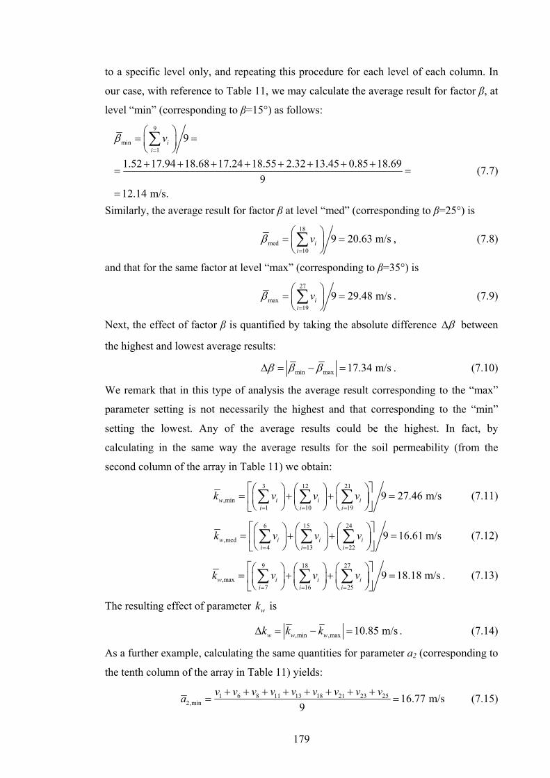
179

to a specific level only, and repeating this procedure for each level of each column. In

our case, with reference to Table 11, we may calculate the average result for factor β, at

level “min” (corresponding to β=15°) as follows:

9

min1

9

1.52 17.94 18.68 17.24 18.55 2.32 13.45 0.85 18.699

12.14 m/s.

ii

vβ=

⎛ ⎞= =⎜ ⎟⎝ ⎠+ + + + + + + +

= =

=

∑

(7.7)

Similarly, the average result for factor β at level “med” (corresponding to β=25°) is

18

med10

9 20.63 m/sii

vβ=

⎛ ⎞= =⎜ ⎟⎝ ⎠∑ , (7.8)

and that for the same factor at level “max” (corresponding to β=35°) is

27

max19

9 29.48 m/sii

vβ=

⎛ ⎞= =⎜ ⎟⎝ ⎠∑ . (7.9)

Next, the effect of factor β is quantified by taking the absolute difference βΔ between

the highest and lowest average results:

min max 17.34 m/sβ β βΔ = − = . (7.10)

We remark that in this type of analysis the average result corresponding to the “max”

parameter setting is not necessarily the highest and that corresponding to the “min”

setting the lowest. Any of the average results could be the highest. In fact, by

calculating in the same way the average results for the soil permeability (from the

second column of the array in Table 11) we obtain:

3 12 21

,min1 10 19

9 27.46 m/sw i i ii i i

k v v v= = =

⎡ ⎤⎛ ⎞ ⎛ ⎞ ⎛ ⎞= + + =⎢ ⎥⎜ ⎟ ⎜ ⎟ ⎜ ⎟

⎝ ⎠ ⎝ ⎠ ⎝ ⎠⎣ ⎦∑ ∑ ∑ (7.11)

6 15 24

,med4 13 22

9 16.61 m/sw i i ii i i

k v v v= = =

⎡ ⎤⎛ ⎞ ⎛ ⎞ ⎛ ⎞= + + =⎢ ⎥⎜ ⎟ ⎜ ⎟ ⎜ ⎟

⎝ ⎠ ⎝ ⎠ ⎝ ⎠⎣ ⎦∑ ∑ ∑ (7.12)

9 18 27

,max7 16 25

9 18.18 m/sw i i ii i i

k v v v= = =

⎡ ⎤⎛ ⎞ ⎛ ⎞ ⎛ ⎞= + + =⎢ ⎥⎜ ⎟ ⎜ ⎟ ⎜ ⎟⎝ ⎠ ⎝ ⎠ ⎝ ⎠⎣ ⎦∑ ∑ ∑ . (7.13)

The resulting effect of parameter wk is

,min ,max 10.85 m/sw w wk k kΔ = − = . (7.14)

As a further example, calculating the same quantities for parameter a2 (corresponding to

the tenth column of the array in Table 11) yields:

1 6 8 11 13 18 21 23 252,min 16.77 m/s

9v v v v v v v v va + + + + + + + +

= = (7.15)

180

2 4 9 12 14 16 19 24 262,med 24.73 m/s

9v v v v v v v v va + + + + + + + +

= = (7.16)

3 5 7 10 15 17 20 22 272,max 20.75 m/s

9v v v v v v v v va + + + + + + + +

= = (7.17)

The resulting effect of parameter a2 is smaller than the previous two:

2 2,min 2,med 7.96 m/sa a aΔ = − = . (7.18)

The same procedure is followed for each of the remaining 10 parameters of Table 11,

and the results are summarised in the response table (Table 12).

The next step is to identify the strong effects, by ranking the factors from the largest to

the smallest absolute difference. This is done in the last row of Table 12, and constitutes

the main result of our parametric analysis.

A rule of thumb of level average analysis is to consider roughly the top half of the

ranked parameters to have a significant impact on the results (Peace, 1993). We may

consider the top-five factors as those that surely have a significant influence in the slide

velocity, namely (1) the static friction-softening rate a1, (2) the slope inclination β, (3)

the soil permeability kw, (4) the dynamic residual friction angle rdφ and (5) the slide

thickness H. This choice is demonstrated to be a valid one by the reliability check

performed in the next section.

7.4.2.2. Reliability check

It is now possible to perform a check on the reliability of our statistical study by

computing an estimate of the predicted response based on the above selected levels of

the dominant parameters (Peace, 1993).

First, we compute the overall average v from the results of Table 11 as

27

120.75 m/si

iv v

=

= =∑ . (7.19)

Next, we calculate a predicted average velocity v ∗ , quantity that incorporates the effect

on the overall average of each one of the 5 dominant factors (Peace, 1993):

( ) ( ) ( )( ) ( )

1,max max ,min

,min max 56.22 m/s

w

rd

v v a v v k v

v H v

β

φ

∗ = + − + − + − +

+ − + − = (7.20)

In other words, v ∗ is the average v plus all the fluctuations from the average v caused

by setting the dominant parameters to their most influential values. Since all such

fluctuations are positive, v ∗ is larger than v . The numerical results from the most

influential parameter settings employed in (7.20), corresponding to the lowest setting

181

for kw and rdφ and the highest setting for a1, β and H, are shaded in Table 12. By

calculating v ∗ we statistically simulate the case scenario that maximises the slide

velocity, thus providing a prediction for the most dangerous parameters settings.

The final step of our reliability check is to conduct a confirmation run with the infinite

slope code, by adopting the most influential parameter settings identified above while

setting all remaining parameters to their mid-range level (Table 13). Our parametric

analysis can be considered successful if the result cv of the confirmation run is higher

than the overall average v , and reasonably close to the prediction average v ∗ .

The velocity after 10s from triggering resulting from our confirmation run is

51.2cv = m/s. We observe that this value is very close to that calculated in (7.20),

especially if compared to the much larger fluctuations from the average exhibited by the

results of Table 11.

In order to check the validity of our choice to consider only the top five parameters in

the ranking of Table 12 as the significant ones in the catastrophic evolution of a slide,

we can now consider significant the top seven parameters instead, thus including also

factors 2a and κ in the calculation of the prediction average, and check whether their

impact is strong enough to yield a prediction average closer to the confirmation run’s

result. Following the above outlined procedure, in this case we obtain 64.4v ∗ = m/s.

The confirmation run, carried out by adopting the most influential parameter settings of

the above top seven parameters, yields 52cv = m/s. The much wider discrepancy

between these two values corroborates our initial choice of considering significant only

the first 5 factors.

We may conclude that indeed, the important factors in making a slope prone to

catastrophic failure are a1, β, kw, rdφ and H.

7.4.2.3. Discussion of the results

The outcome of our parametric study is the ranking in order of importance of the

involved landslide properties in causing catastrophic sliding, as reported in Section

7.4.2.1: among all the classified parameters, the first 5 can be deemed to have a key role

in maximising the landslide velocity.

182

Table 11. Orthogonal array for the infinite slide parametric analysis.

Exp/

para

mβ

k wH

dγ

φ cs

φrs

φ rd

a 1a 2

Γk

λ Re

sults

: vel

ocity

v

afte

r 10s

(m/s

)1

151.

00E-

135

3.00

E-04

1.00

E-03

2010

41.

00E-

051.

00E-

052.

83.

00E-

029.

00E-

021.

522

151.

00E-

135

3.00

E-04

1.00

E-02

2515

81.

00E-

011.

00E-

013.

24.

50E-

021.

70E-

0117

.94

315

1.00

E-13

53.

00E-

041.

00E-

0132

2010

1.00

E+03

1.00

E+03

3.8

6.00

E-02

2.60

E-01

18.6

84

151.

00E-

0913

01.

00E-

031.

00E-

0320

108

1.00

E-01

1.00

E-01

3.8

6.00

E-02

2.60

E-01

17.2

45

151.

00E-

0913

01.

00E-

031.

00E-

0225

1510

1.00

E+03

1.00

E+03

2.8

3.00

E-02

9.00

E-02

18.5

56

151.

00E-

0913

01.

00E-

031.

00E-

0132

204

1.00

E-05

1.00

E-05

3.2

4.50

E-02

1.70

E-01

2.32

715

1.00

E-06

250

3.00

E-03

1.00

E-03

2010

101.

00E+

031.

00E+

033.

24.

50E-

021.

70E-

0113

.45

815

1.00

E-06

250

3.00

E-03

1.00

E-02

2515

41.

00E-

051.

00E-

053.

86.

00E-

022.

60E-

010.

859

151.

00E-

0625

03.

00E-

031.

00E-

0132

208

1.00

E-01

1.00

E-01

2.8

3.00

E-02

9.00

E-02

18.6

910

251.

00E-

1313

03.

00E-

031.

00E-

0325

204

1.00

E-01

1.00

E+03

2.8

4.50

E-02

2.60

E-01

29.2

511

251.

00E-

1313

03.

00E-

031.

00E-

0232

108

1.00

E+03

1.00

E-05

3.2

6.00

E-02

9.00

E-02

33.4

512

251.

00E-

1313

03.

00E-

031.

00E-

0120

1510

1.00

E-05

1.00

E-01

3.8

3.00

E-02

1.70

E-01

13.7

513

251.

00E-

0925

03.

00E-

041.

00E-

0325

208

1.00

E+03

1.00

E-05

3.8

3.00

E-02

1.70

E-01

20.0

214

251.

00E-

0925

03.

00E-

041.

00E-

0232

1010

1.00

E-05

1.00

E-01

2.8

4.50

E-02

2.60

E-01

7.8

1525

1.00

E-09

250

3.00

E-04

1.00

E-01

2015

41.

00E-

011.

00E+

033.

26.

00E-

029.

00E-

0233

.36

1625

1.00

E-06

51.

00E-

031.

00E-

0325

2010

1.00

E-05

1.00

E-01

3.2

6.00

E-02

9.00

E-02

4.00

E-05

1725

1.00

E-06

51.

00E-

031.

00E-

0232

104

1.00

E-01

1.00

E+03

3.8

3.00

E-02

1.70

E-01

35.8

518

251.

00E-

065

1.00

E-03

1.00

E-01

2015

81.

00E+

031.

00E-

052.

84.

50E-

022.

60E-

0112

.15

1935

1.00

E-13

250

1.00

E-03

1.00

E-03

3215

41.

00E+

031.

00E-

012.

86.

00E-

021.

70E-

0153

.25

2035

1.00

E-13

250

1.00

E-03

1.00

E-02

2020

81.

00E-

051.

00E+

033.

23.

00E-

022.

60E-

0133

.89

2135

1.00

E-13

250

1.00

E-03

1.00

E-01

2510

101.

00E-

011.

00E-

053.

84.

50E-

029.

00E-

0245

.422

351.

00E-

095

3.00

E-03

1.00

E-03

3215

81.

00E-

051.

00E+

033.

84.

50E-

029.

00E-

021.

1123

351.

00E-

095

3.00

E-03

1.00

E-02

2020

101.

00E-

011.

00E-

052.

86.

00E-

021.

70E-

010.

6924

351.

00E-

095

3.00

E-03

1.00

E-01

2510

41.

00E+

031.

00E-

013.

23.

00E-

022.

60E-

0148

.38

2535

1.00

E-06

130

3.00

E-04

1.00

E-03

3215

101.

00E-

011.

00E-

053.

23.

00E-

022.

60E-

0134

.53

2635

1.00

E-06

130

3.00

E-04

1.00

E-02

2020

41.

00E+

031.

00E-

013.

84.

50E-

029.

00E-

0245

.51

2735

1.00

E-06

130

3.00

E-04

1.00

E-01

2510

81.

00E-

051.

00E+

032.

86.

00E-

021.

70E-

012.

58

183

Table 12. Response table of our 13-parameter landslide model Taguchi analysis.

Level/par. β kw H d γ φcs φrs φrd a1 a2 Γ k λMin 12.14 27.46 15.15 20.22 18.93 19.06 21.53 27.81 7.09 16.77 16.05 25.02 21.95Med 20.63 16.61 21.91 24.29 21.61 20.33 20.61 17.45 25.88 24.73 22.83 19.44 17.76Max 29.48 18.18 25.19 17.74 21.70 22.85 18.78 16.98 29.27 20.75 22.05 17.79 22.53

Effect of parameter

(Delta)17.34 10.85 10.04 6.56 2.77 3.79 2.74 10.83 22.18 7.96 6.77 7.23 4.77

Ranking 2 3 5 9 12 11 13 4 1 6 8 7 10

RESPONSE TABLE (slide velocity in m/s after t=10 seconds from triggering)

Table 13. Parameter settings for the confirmation run of our general Taguchi analysis.

Exp/param βmax kw,min Hmax dmed γmed φcs,med φrs,med φrd,min a1,max a2,med Γmed kmed λmed

Confirmation run 35 1.00E-13 250 1.00E-003 1.00E-002 25 15 4 1.00E+03 0.1 3.2 4.50E-02 1.70E-01

The worst-case scenario for a planar slide is represented by the parameter combination

of Table 13: a potentially unstable slope is bound to be most catastrophic if the soil’s

static softening rate, the inclination and the thickness of the slope are very large, and the

soil’s permeability and dynamic residual friction angle are very small. Of these five

properties, 1a , β and rdφ are independent of thermal effects, thus constituting

important factors in standard landslide analyses as well. The strong influence of 1a and

rdφ is explained by observing that while thermal pressurisation needs a certain time to

cause liquefaction, material friction-softening fully develops within a few centimetres of

displacement after the initiation of movement (cf. Section 6.3.5, and Vardoulakis,

2002a). Besides, the slope inclination is understandably crucial in the landslide

dynamics as it determines the magnitude of the driving force. On the other hand,

parameters kw and H deserve more attention, as they have been introduced by the

thermo-mechanical model, and are not normally considered in landslide prevention

practice. The most important one of the two parameters is kw, which affects pore

pressure diffusion: a low soil permeability implies a poor dissipation of the excess pore

pressure within the shearband, thus promoting the reduction of shear resistance. The

influence of parameter H, determining the amount of dissipation as anticipated in

Section 7.1, is plausibly second to permeability: despite the amount of frictional heat

that may be produced, if pore pressure does not build up no strength loss will be caused

(in the absence of friction softening).

The above observations are useful as a guidance for field investigations on potentially

unstable large slopes: by measuring or estimating the aforementioned five key

184

properties, it is possible to determine whether or not the slope is bound to evolve

catastrophically. The slope’s inclination and depth of the slip plane may be easier to

detect, while for 1a and rdφ it is necessary to collect samples and run laboratory tests,

more specifically dynamic ring shear tests such as those performed by Tika and

Hutchinson (1999). Despite the possibility to measure the permeability kw in-situ, this

should be avoided since the presence of fractures would lead to an overestimation of the

shearband permeability, in turn leading to underestimation of thermal pressurisation.

Moreover, the permeability of most clays is likely to decrease as the soil approaches

residual state, due to the alignment of the platy particles parallel to the direction of

motion (cf. Section 7.2.2). Thus, in order to obtain more sensible information it might

be more appropriate to run a laboratory permeability test on a sample that has

previously undergone prolonged shearing.

7.4.3. A Taguchi analysis focusing on thermo-mechanical effects

The analysis of Section 7.4.2.1 involved 13 parameters of different nature, that can be

grouped into ‘thermo-mechanical’ and ‘standard’ parameters, depending on whether or

not they are relevant of a thermo-mechanical analysis only, as opposed to a standard

stability analysis. Some of the thermo-mechanical parameters, namely the shearband

thickness d and the thermal softening parameter γ, have been left out of the list of key

factors, as the level average analysis showed that their influence is weak. However, in

cases where the standard parameters assume ‘non-catastrophic’ values (i.e., values that

minimise the velocity such as moderate/absent friction softening and moderate slope

angle) the thermo-mechanical factors will have a yet more important role in the

catastrophic evolution of a slide. In order to corroborate the conclusions drawn in

Section 7.4.2.3, it is useful to carry out a parametric study focused on the thermo-

mechanical parameters only. This will also allow us to assess whether these parameters

can be decisive in making catastrophic a slide that would be otherwise (i.e., with a

standard analysis) predicted to be non-catastrophic. The analysis can be performed by

means of a standard ( )49 3L orthogonal array, where thermo-mechanical factors kw, H,

d, γ are varied within the relevant ranges while the remaining 9 factors of Table 8 are

kept constant.

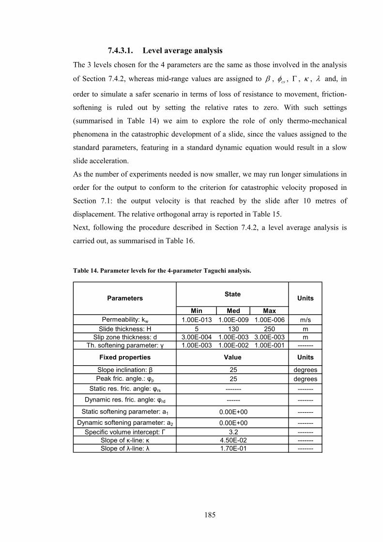
185

7.4.3.1. Level average analysis

The 3 levels chosen for the 4 parameters are the same as those involved in the analysis

of Section 7.4.2, whereas mid-range values are assigned to β , csφ , Γ , κ , λ and, in

order to simulate a safer scenario in terms of loss of resistance to movement, friction-

softening is ruled out by setting the relative rates to zero. With such settings

(summarised in Table 14) we aim to explore the role of only thermo-mechanical

phenomena in the catastrophic development of a slide, since the values assigned to the

standard parameters, featuring in a standard dynamic equation would result in a slow

slide acceleration.

As the number of experiments needed is now smaller, we may run longer simulations in

order for the output to conform to the criterion for catastrophic velocity proposed in

Section 7.1: the output velocity is that reached by the slide after 10 metres of

displacement. The relative orthogonal array is reported in Table 15.

Next, following the procedure described in Section 7.4.2, a level average analysis is

carried out, as summarised in Table 16.

Table 14. Parameter levels for the 4-parameter Taguchi analysis.

Min Med MaxPermeability: kw 1.00E-013 1.00E-009 1.00E-006 m/s

Slide thickness: H 5 130 250 mSlip zone thickness: d 3.00E-004 1.00E-003 3.00E-003 m

Th. softening parameter: γ 1.00E-003 1.00E-002 1.00E-001 -------

Slope inclination: β 25 degreesPeak fric. angle.: φp 25 degrees

Static res. fric. angle: φrs ------- -------Dynamic res. fric. angle: φrd ------ -------

Static softening parameter: a1 0.00E+00 -------Dynamic softening parameter: a2 0.00E+00 -------

Specific volume intercept: Γ 3.2 -------Slope of κ-line: κ 4.50E-02 -------Slope of λ-line: λ 1.70E-01 -------

Fixed properties Value Units

State UnitsParameters

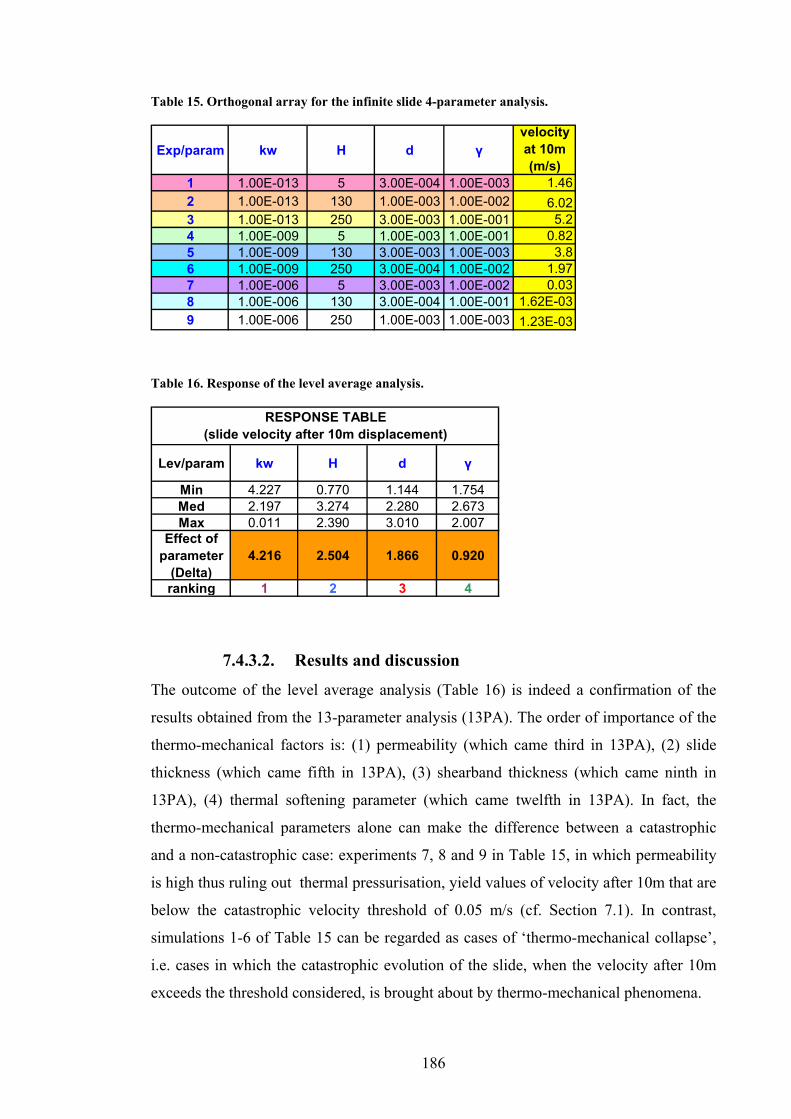
186

Table 15. Orthogonal array for the infinite slide 4-parameter analysis.

Exp/param kw H d γvelocity at 10m (m/s)

1 1.00E-013 5 3.00E-004 1.00E-003 1.462 1.00E-013 130 1.00E-003 1.00E-002 6.023 1.00E-013 250 3.00E-003 1.00E-001 5.24 1.00E-009 5 1.00E-003 1.00E-001 0.825 1.00E-009 130 3.00E-003 1.00E-003 3.86 1.00E-009 250 3.00E-004 1.00E-002 1.977 1.00E-006 5 3.00E-003 1.00E-002 0.038 1.00E-006 130 3.00E-004 1.00E-001 1.62E-039 1.00E-006 250 1.00E-003 1.00E-003 1.23E-03

Table 16. Response of the level average analysis.

Lev/param kw H d γ

Min 4.227 0.770 1.144 1.754Med 2.197 3.274 2.280 2.673Max 0.011 2.390 3.010 2.007

Effect of parameter

(Delta)4.216 2.504 1.866 0.920

ranking 1 2 3 4

RESPONSE TABLE (slide velocity after 10m displacement)

7.4.3.2. Results and discussion

The outcome of the level average analysis (Table 16) is indeed a confirmation of the

results obtained from the 13-parameter analysis (13PA). The order of importance of the

thermo-mechanical factors is: (1) permeability (which came third in 13PA), (2) slide

thickness (which came fifth in 13PA), (3) shearband thickness (which came ninth in

13PA), (4) thermal softening parameter (which came twelfth in 13PA). In fact, the

thermo-mechanical parameters alone can make the difference between a catastrophic

and a non-catastrophic case: experiments 7, 8 and 9 in Table 15, in which permeability

is high thus ruling out thermal pressurisation, yield values of velocity after 10m that are

below the catastrophic velocity threshold of 0.05 m/s (cf. Section 7.1). In contrast,

simulations 1-6 of Table 15 can be regarded as cases of ‘thermo-mechanical collapse’,

i.e. cases in which the catastrophic evolution of the slide, when the velocity after 10m

exceeds the threshold considered, is brought about by thermo-mechanical phenomena.

187

It is now worth recalling a rule of thumb of level average analysis (Section 7.4.2.1): due

to the statistical nature of the results, only about half of the parameters in the ranking

can be considered to have a significant effect (Peace, 1993). By examining the results of

the above 4-parameter analysis in light of this criterion, we have confirmation that the

only two properties which are worth determining for assessing the danger of thermo-

mechanical collapse are the permeability of the soil and the thickness of the slide.

Fortunately, these two properties coincide with the best-established and easiest ones to

quantify in the field. The measurement of H implies the detection of an existing rupture

surface or a reasonable assumption, based on local geology and in-situ conditions, of

where a rupture surface would be expected to develop. The permeability kw of the soil

expected to be involved in shearing can be estimated by means of a specific

permeability test (cf. Section 7.4.2.3). On the other hand, the shearband thickness is of

uncertain determination and has hardly ever been directly measured (e.g. see

Morgenstern and Tschalenko, 1967, Vardoulakis, 2002a and Section 2.3.4) and

parameter γ would require non-standard thermally controlled triaxial tests (Laloui and

Cekerevac, 2003).

The above observations allow us to conclude that, in order to assess whether a

potentially unstable slope is bound to exhibit thermo-mechanical collapse, the depth of

the slip plane and the permeability of the soil therein should be estimated or measured.

We may estimate, as a guidance, that if the permeability falls in the (lower) range 9 1310 10wk− −≤ ≤ m/s and the depth in the (higher) range 130 250H≤ ≤ m, there is a

high risk of thermo-mechanical collapse; thus the slide may assume unexpectedly high

velocities, despite possibly retaining its coherence of mass, and pose a higher threat to

populations and the environment than expected from a traditional stability analysis. In

fact, landslides of this type constitute a higher threat not only because, once rupture has

taken place, they allow less time for evacuation of the population, but also for the

potential creation of tsunamis or flood surges in case the mass comes into contact with a

body of water.

On the other hand, it is rather difficult to employ the thermo-mechanical model to

accurately predict the time evolution of the slide’s velocity in the real case of a

potentially unstable slope. This is because of the difficulty and cost of measuring all the

relevant parameters before a landslide takes place, but also because a one-dimensional

model cannot account for the numerous morphological constraints and inhomogeneities

that influence the dynamical evolution of a slide. Nevertheless, for civil protection

188

purposes it may be enough to calculate the order of magnitude of velocity that the slide

can reach after a certain displacement. This could be done, within limits (Section 7.5),

with the thermo-mechanical model presented in this work.

7.5. Limitations of the infinite slope model

Although most of the limitations of the infinite slope thermo-mechanical model have

been already highlighted throughout this work, it is worth summarising them here, in

order to better identify the future direction of research in this subject (cf. Chapter 8).

An evident drawback of the model is its inability to capture creep, which often precedes

catastrophic collapse in large-scale, deep-seated landslides (cf. Section 2.1.4.2). In fact,

the structure of the dynamic equation does not allow any velocity reduction or rate

effects. For this reason, on the one hand the model is unable to predict stick-slip or

decelerated types of movement, and on the other hand it cannot interpret excessively

long run-out sliding, in which possibly viscous effects (along with topographical

constraints) may prevent the velocity from increasing indefinitely. The model is reliable

for interpreting the slide dynamics within a displacement interval that greatly depends

on the specific case under study, but can be set as an example to about 200 metres for

large, deep-seated landslides like Vajont. Another reason for which the model cannot be

employed for velocity predictions beyond a certain run-out distance is that, rather

frequently, beyond a threshold displacement, large-scale landslides transform into a

flow-like phenomenon, implying the end of validity for the hypothesis of coherence of

mass that allowed us to employ the block-on-slope model.

Furthermore, the inability of our model to capture creep is linked to the random nature

of the triggering condition for the dynamic equation: a minute decrease φ′−Δ of the

mobilised friction angle (Section 6.1.1) or a minute increase HuΔ of the pore pressure

(Section 7.3) is imposed to trigger the slide movement. Numerical experimentation was

performed to assess the sensitivity of the model response to such incipient failure

conditions. It was found that the predicted 10sv (velocity after 10s from triggering) is

substantially affected by the value chosen for HuΔ if thermal pressurisation is not

considered, i.e. in cases when the calculated 10sv is very small (order of magnitude of

10-6-10-4 m/s), and negligibly affected when pressurisation is active and the calculated

10sv is large (order of magnitude of 10 m/s). More specifically, for a variation of HuΔ

from 10-5 to 1 Pa, we obtain a variation in the predicted velocity of 0.01-5% (thus

189

negligible to our purposes) for the cases when thermal pressurisation is considered, and

of more than 100% when thermal pressurisation is ruled out. The sensitivity to the

triggering condition HuΔ in any case diminishes for increasing slide thickness H and

overburden’s unit weight sγ , as can be deduced by looking at the last term on the right

hand side of Equation (7.1).

The above results make us reconsider the values of velocity after ten metres calculated

in the last three rows of Table 15, when high permeability excludes thermal

pressurisation, and lead us to conclude that although the calculated order of magnitudes

are reliable, the values themselves are not. This in turn justifies our reluctance in

adopting a (yet difficult to establish) threshold value for a catastrophic sliding velocity

in our analysis (cf. Section 7.1); and further confirms that the most fruitful use of our

model is estimating, by looking at a few key parameters, whether or not catastrophic

collapse can occur, rather than predicting the timescale of the phenomenon.

We should finally remark that the model cannot be trusted if the predicted temperature

exceeds the vaporisation threshold at the given pressure (cf. Section 5.5.7.1), as the

thermo-dynamical assumptions behind the governing equations will cease to be valid.

This has been checked for our simulations and proved never to be the case, although it

might happen for cases of very thick and heavy overburden, higher friction angles and

thinner shearbands. In such cases, the calculated values should be considered invalid as

soon as vaporisation starts. This, however, would not necessarily affect the indicative

value of the velocity predictions, as in most cases of thermo-mechanical collapse the

acceleration of the slide evolves in the first few seconds and soon becomes constant,

possibly before the temperature reaches the vaporisation threshold.

190

Chapter 8. Conclusions and future work

8.1. General conclusions

In this work we investigated the role of frictional heating in the development of

catastrophic landslides. In particular:

• Landslide case histories and existing landslide models were critically reviewed,

special attention being given to catastrophic landslides. For terrestrial landslides,

typical ranges of certain soil properties such as residual static friction angles and

of in-situ conditions like slope inclinations were identified, whereas other

parameters (e.g. thermal-friction softening rates, residual dynamic friction

angles) were found to be scarcely available in the literature. Furthermore, the

most representative cases of coherent catastrophic landsliding were identified,

among which the best-documented ones turned out to be the Vajont and

Jiufengershan cases.

• Existing thermo-elasto-plastic constitutive soil models were reviewed. Due to its

simpler formulation and the fewer material parameters, the model proposed by

Laloui et al. (2005) was found to be the most suitable to be incorporated in a

thermo-mechanical landslide model.

• A generalised thermo-plastic constitutive model was developed, based on re-

deriving the constitutive law proposed by Laloui et al. (2005) in a standard

plasticity framework, with a general stress space formulation. The model was

then discretised using a refined explicit scheme, and validated by reproducing

experimental thermo-mechanical loading paths.

• An improved landslide model based on that proposed by Vardoulakis (2002)

was developed accounting for frictional heating, thermal pressurisation and

including the above thermo-plastic generalised constitutive law for the soil. The

model was discretised using an explicit scheme, and validated by successfully

back-analysing the Vajont landslide. It also emerged that the newly introduced

thermal friction softening mechanism is of secondary importance to the

catastrophic acceleration of a slide compared to the better established

mechanisms of static and dynamic material friction softening.

191

• The landslide model was generalised to an infinite slope geometry, discretised

and validated by back-analysing the translational catastrophic landslide case of

Jiufengershan.

• A parametric study to systematically investigate the development of catastrophic

failure in uniform slopes was carried out. It was found that the most influential

parameters in promoting catastrophic collapse are (1) the static friction-softening

rate a1, (2) the slope inclination β, (3) the soil permeability kw, (4) the dynamic

residual friction angle rdφ and (5) the overburden thickness H. The most

dangerous situation is when a1, β and H are very large and kw and rdφ are very

low. Of the above, ‘thermo-mechanical parameters’ kw and H deserve more

attention as they have been introduced by the thermo-mechanical model and are

not normally considered in standard stability analyses of uniform slopes. A

second parametric study was performed to demonstrate that thermo-mechanical

parameters alone can make a difference between a relatively non-catastrophic

event and a catastrophic one. Hence, further insight into the design of landslide

risk mitigation measures is gained if, in addition to the standard site

investigations, the permeability of the soil is measured and the depth of an

existing or expected failure surface is measured or estimated respectively.

8.2. Recommendations for further research

A major limitation of the model developed in this work is that it disregards a landslide’s

creep-like activity before the final collapse phase, thus being unable to predict the

overall timescale of a slide’s failure. This may be overcome by integrating the model

developed with another one that is able to interpret creep from a thermo-mechanical

point of view, such as the analytical asymptotic model proposed by Veveakis et al.

(2007). Coupling the two models would require special attention to the critical phase of

transition between the creeping regime described by one model and the final collapse

described by the other. A crack propagation analysis would probably be required to

model the formation of the shearband and the evolution of its thickness.

A further enhancement could be brought about by generalising the above thermo-

mechanical model to a 2-D finite element analysis. This may also involve the

implementation of interface elements, for correctly modelling the interface between the

two substructures constituted by the bedrock and the overburden. The shearband would

192

be confined within the interface element and the same constitutive model for the

interface element and the surrounding soil could be used.

The above improvements could lead to the development of a more general modelling

tool, able to capture the dynamic emergence of progressive thermo-mechanical failure,

from the inception of rupture to the final catastrophic collapse, in slopes of arbitrary

geometry due to different initiation events.

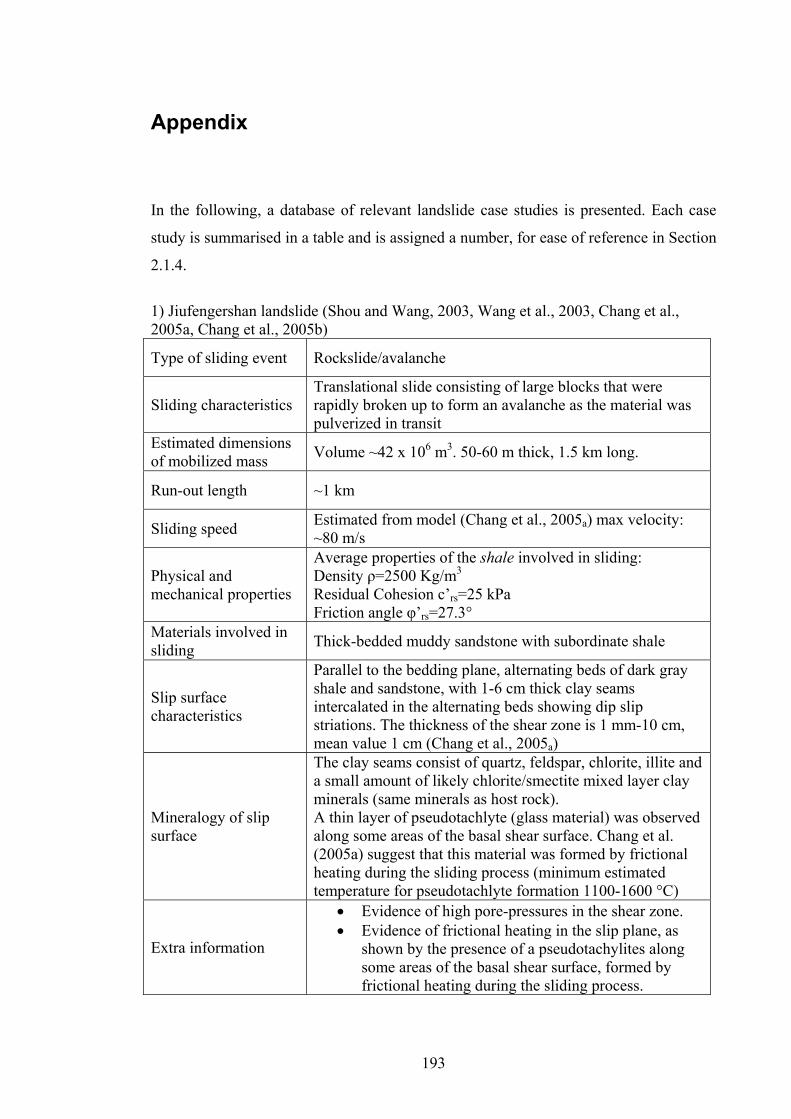
193

Appendix

In the following, a database of relevant landslide case studies is presented. Each case

study is summarised in a table and is assigned a number, for ease of reference in Section

2.1.4.

1) Jiufengershan landslide (Shou and Wang, 2003, Wang et al., 2003, Chang et al., 2005a, Chang et al., 2005b)

Type of sliding event Rockslide/avalanche

Sliding characteristics Translational slide consisting of large blocks that were rapidly broken up to form an avalanche as the material was pulverized in transit

Estimated dimensions of mobilized mass Volume ~42 x 106 m3. 50-60 m thick, 1.5 km long.

Run-out length ~1 km

Sliding speed Estimated from model (Chang et al., 2005a) max velocity: ~80 m/s

Physical and mechanical properties

Average properties of the shale involved in sliding: Density ρ=2500 Kg/m3 Residual Cohesion c’rs=25 kPa Friction angle φ’rs=27.3°

Materials involved in sliding Thick-bedded muddy sandstone with subordinate shale

Slip surface characteristics

Parallel to the bedding plane, alternating beds of dark gray shale and sandstone, with 1-6 cm thick clay seams intercalated in the alternating beds showing dip slip striations. The thickness of the shear zone is 1 mm-10 cm, mean value 1 cm (Chang et al., 2005a)

Mineralogy of slip surface

The clay seams consist of quartz, feldspar, chlorite, illite and a small amount of likely chlorite/smectite mixed layer clay minerals (same minerals as host rock). A thin layer of pseudotachlyte (glass material) was observed along some areas of the basal shear surface. Chang et al. (2005a) suggest that this material was formed by frictional heating during the sliding process (minimum estimated temperature for pseudotachlyte formation 1100-1600 °C)

Extra information

• Evidence of high pore-pressures in the shear zone. • Evidence of frictional heating in the slip plane, as

shown by the presence of a pseudotachylites along some areas of the basal shear surface, formed by frictional heating during the sliding process.

194

2) La Clapiere landslide (Sornette et al., 2004, Helmstetter et al., 2004, Cappa et al., 2004, Follacci et al., 1988)

Type of sliding event Rockslide

Sliding characteristics Slow, accelerating creep of coherent mass for decades. Rotational-like sliding shape (Follacci et al., 1988), multiple progressive fracturing.

Estimated dimensions of mobilized mass

Volume ~50 x 106 m3. Width ~1000 m. 50 m high escarpment.

Run-out length <100 m

Sliding speed

• Increase from 0.5 m/year in the 1950-1960 period to 1.5 m/year in the 1975-1982 period.

• Dramatic increase between 1986 and 1988, up to 80 mm/day in summer 1987 and 90 mm/day in October 1987.

• Decrease and stabilization in displacement rate ( to some meters/year) since 1988 (Sornette et al., 2004)

Physical and mechanical properties NA

Materials involved in sliding Mostly gneiss rock

Slip surface characteristics

No defined slip surface. An 80 m-thick gneiss bed provides a stronger level compared with the rest of relatively weak and fractured gneiss; the two lithological entities are characterized by a change in mica content which is associated with a change of the peak strength (Follacci et al., 1988).

Mineralogy of slip surface NA

3) Ok Ma dam 1984 landslide (Griffiths et al., 2004)

Type of sliding event Rock and earth slide

Sliding characteristics Repeated, short-reach downslope movement of coherent mass on pre-existing shear surfaces

Estimated dimensions of mobilized mass Volume ~35 x 106 m3.

Run-out length ~21 m

Sliding speed Max. 5.2 m/h

Physical and mechanical properties

Average properties of some shear surfaces in the sliding mass: Assumed residual cohesion c’rs=0 kPa Static residual friction coefficient φ’rs=16° Liquid limit=38% Plastic limit=23%

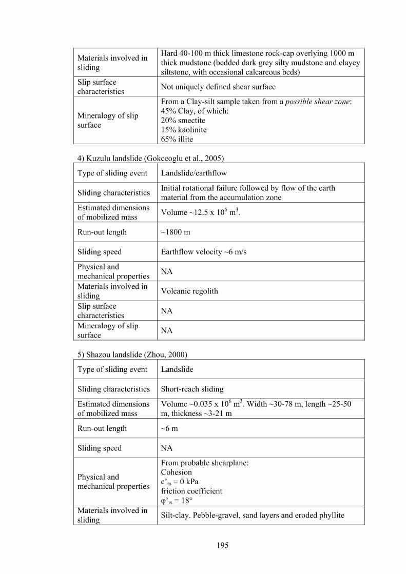
195

Materials involved in sliding

Hard 40-100 m thick limestone rock-cap overlying 1000 m thick mudstone (bedded dark grey silty mudstone and clayey siltstone, with occasional calcareous beds)

Slip surface characteristics Not uniquely defined shear surface

Mineralogy of slip surface

From a Clay-silt sample taken from a possible shear zone: 45% Clay, of which: 20% smectite 15% kaolinite 65% illite

4) Kuzulu landslide (Gokceoglu et al., 2005)

Type of sliding event Landslide/earthflow

Sliding characteristics Initial rotational failure followed by flow of the earth material from the accumulation zone

Estimated dimensions of mobilized mass Volume ~12.5 x 106 m3.

Run-out length ~1800 m

Sliding speed Earthflow velocity ~6 m/s

Physical and mechanical properties NA

Materials involved in sliding Volcanic regolith

Slip surface characteristics NA

Mineralogy of slip surface NA

5) Shazou landslide (Zhou, 2000)

Type of sliding event Landslide

Sliding characteristics Short-reach sliding

Estimated dimensions of mobilized mass

Volume ~0.035 x 106 m3. Width ~30-78 m, length ~25-50 m, thickness ~3-21 m

Run-out length ~6 m

Sliding speed NA

Physical and mechanical properties

From probable shearplane: Cohesion c’rs = 0 kPa friction coefficient φ’rs = 18°

Materials involved in sliding Silt-clay. Pebble-gravel, sand layers and eroded phyllite

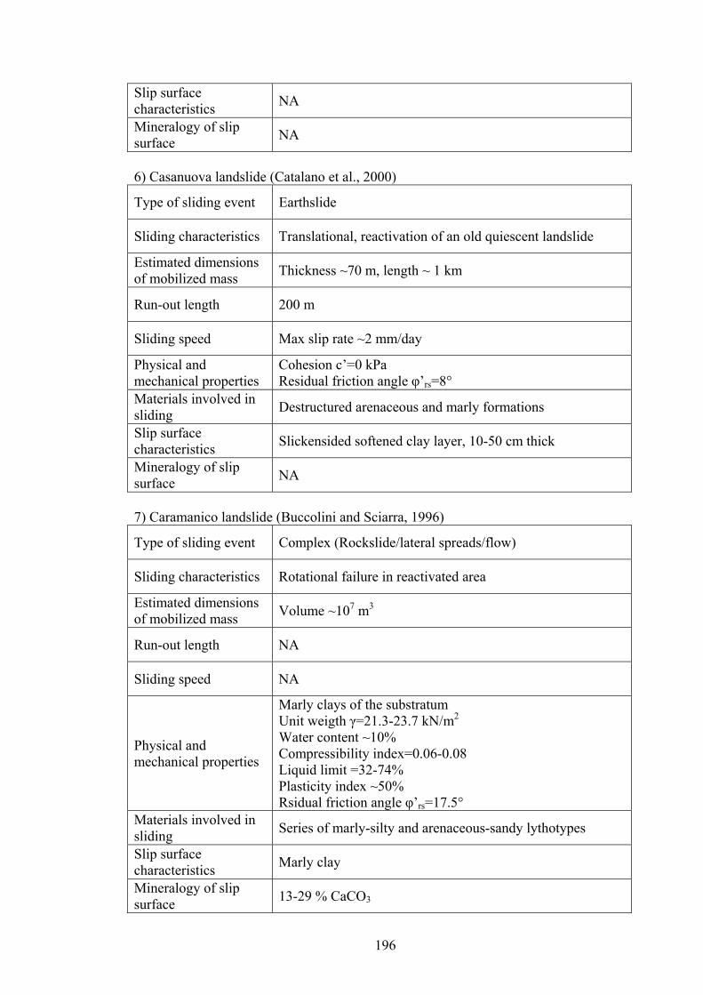
196

Slip surface characteristics NA

Mineralogy of slip surface NA

6) Casanuova landslide (Catalano et al., 2000)

Type of sliding event Earthslide

Sliding characteristics Translational, reactivation of an old quiescent landslide

Estimated dimensions of mobilized mass Thickness ~70 m, length ~ 1 km

Run-out length 200 m

Sliding speed Max slip rate ~2 mm/day

Physical and mechanical properties

Cohesion c’=0 kPa Residual friction angle φ’rs=8°

Materials involved in sliding Destructured arenaceous and marly formations

Slip surface characteristics Slickensided softened clay layer, 10-50 cm thick

Mineralogy of slip surface NA

7) Caramanico landslide (Buccolini and Sciarra, 1996)

Type of sliding event Complex (Rockslide/lateral spreads/flow)

Sliding characteristics Rotational failure in reactivated area

Estimated dimensions of mobilized mass Volume ~107 m3

Run-out length NA

Sliding speed NA

Physical and mechanical properties

Marly clays of the substratum Unit weigth γ=21.3-23.7 kN/m2 Water content ~10% Compressibility index=0.06-0.08 Liquid limit =32-74% Plasticity index ~50% Rsidual friction angle φ’rs=17.5°

Materials involved in sliding Series of marly-silty and arenaceous-sandy lythotypes

Slip surface characteristics Marly clay

Mineralogy of slip surface 13-29 % CaCO3

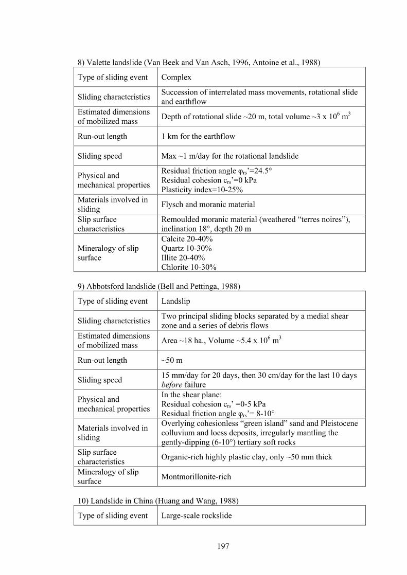
197

8) Valette landslide (Van Beek and Van Asch, 1996, Antoine et al., 1988)

Type of sliding event Complex

Sliding characteristics Succession of interrelated mass movements, rotational slide and earthflow

Estimated dimensions of mobilized mass Depth of rotational slide ~20 m, total volume ~3 x 106 m3

Run-out length 1 km for the earthflow

Sliding speed Max ~1 m/day for the rotational landslide

Physical and mechanical properties

Residual friction angle φrs’=24.5° Residual cohesion crs’=0 kPa Plasticity index=10-25%

Materials involved in sliding Flysch and moranic material

Slip surface characteristics

Remoulded moranic material (weathered “terres noires”), inclination 18°, depth 20 m

Mineralogy of slip surface

Calcite 20-40% Quartz 10-30% Illite 20-40% Chlorite 10-30%

9) Abbotsford landslide (Bell and Pettinga, 1988)

Type of sliding event Landslip

Sliding characteristics Two principal sliding blocks separated by a medial shear zone and a series of debris flows

Estimated dimensions of mobilized mass Area ~18 ha., Volume ~5.4 x 106 m3

Run-out length ~50 m

Sliding speed 15 mm/day for 20 days, then 30 cm/day for the last 10 days before failure

Physical and mechanical properties

In the shear plane: Residual cohesion crs’ =0-5 kPa Residual friction angle φrs’= 8-10°

Materials involved in sliding

Overlying cohesionless “green island” sand and Pleistocene colluvium and loess deposits, irregularly mantling the gently-dipping (6-10°) tertiary soft rocks

Slip surface characteristics Organic-rich highly plastic clay, only ~50 mm thick

Mineralogy of slip surface Montmorillonite-rich

10) Landslide in China (Huang and Wang, 1988)

Type of sliding event Large-scale rockslide

198

Sliding characteristics Coherent translational sliding, then broken up in large blocks

Estimated dimensions of mobilized mass

Area ~0.2 km2., Volume ~31.7 x 106 m3, length ~750 m, width ~300 m.

Run-out length ~550 m

Sliding speed High velocity, not determined

Physical and mechanical properties

Compressive strength of rock mass =18 Mpa Friction angle of the joint corresponding to the slip surface φ’=32°

Materials involved in sliding Granite

Slip surface characteristics Gently inclined (28°) joint set

Mineralogy of slip surface NA

Extra information

• Evidence of high-speed sliding due to long run-out of such a huge rock mass

• Inferred average temperature on the slip surface: 310 °C

• A “block rolling friction mechanism” is assumed to explain the high sliding speed of the rock mass

11) Furre landslide (Hutchinson, 1961)

Type of sliding event Translational earthslide

Sliding characteristics A mainly cohesionless mass slid as a single intact flake on a thin layer of quick clay

Estimated dimensions of mobilized mass

Area ~180,000 m2., Volume ~3 x 106 m3, length ~300 m, width ~850 m.

Run-out length ~90 m

Sliding speed NA

Physical and mechanical properties

Shear surface: Peak friction angle φp’=25°

Materials involved in sliding Post-glacial and deltaic deposits

Slip surface characteristics

Layer of very quick clay, 2-10 cm thick, flat and gently inclined (6°-9°)

Mineralogy of slip surface

Main constituents of the quick clay, in descending order of quantity: Chamosite (of chlorite type) Illite Inactive minerals of quartz and feldspar

12) Usoy landslide (Gaziev, 1984)

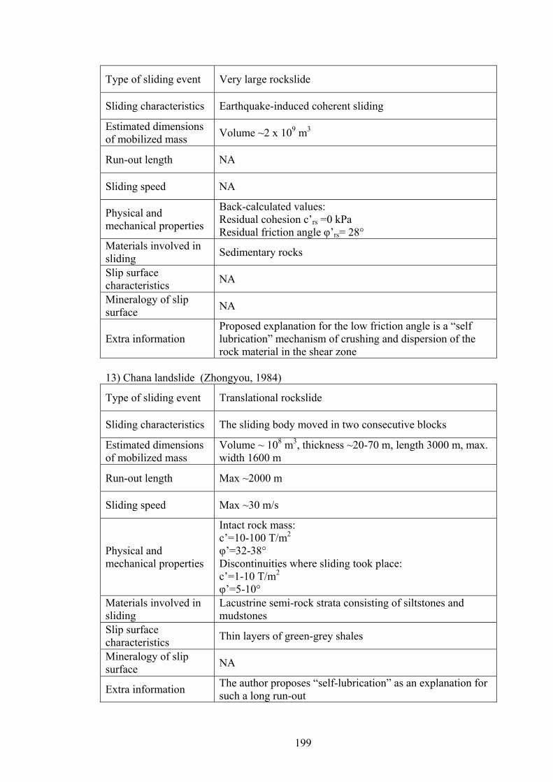
199

Type of sliding event Very large rockslide

Sliding characteristics Earthquake-induced coherent sliding

Estimated dimensions of mobilized mass Volume ~2 x 109 m3

Run-out length NA

Sliding speed NA

Physical and mechanical properties

Back-calculated values: Residual cohesion c’rs =0 kPa Residual friction angle φ’rs= 28°

Materials involved in sliding Sedimentary rocks

Slip surface characteristics NA

Mineralogy of slip surface NA

Extra information Proposed explanation for the low friction angle is a “self lubrication” mechanism of crushing and dispersion of the rock material in the shear zone

13) Chana landslide (Zhongyou, 1984)

Type of sliding event Translational rockslide

Sliding characteristics The sliding body moved in two consecutive blocks

Estimated dimensions of mobilized mass

Volume ~ 108 m3, thickness ~20-70 m, length 3000 m, max. width 1600 m

Run-out length Max ~2000 m

Sliding speed Max ~30 m/s

Physical and mechanical properties

Intact rock mass: c’=10-100 T/m2 φ’=32-38° Discontinuities where sliding took place: c’=1-10 T/m2 φ’=5-10°

Materials involved in sliding

Lacustrine semi-rock strata consisting of siltstones and mudstones

Slip surface characteristics Thin layers of green-grey shales

Mineralogy of slip surface NA

Extra information The author proposes “self-lubrication” as an explanation for such a long run-out

200

14) Landslides in Fukushima, Japan (Okura et al., 2003)

Type of sliding event Earthslides/debris slides

Sliding characteristics Long run-out translational movement

Estimated dimensions of mobilized mass Volumes ranging from 102 to 1.5 x 103 m3

Run-out length NA

Sliding speed NA

Physical and mechanical properties

Average properties of slip surfaces: Density ρ=0.55-0.85 g/cm3 Friction coefficient μ’=0.5-0.8

Materials involved in sliding

Thick layer of welded pyroclastic rock overlaid with a loam layer of 0.5-2 m thickness.

Slip surface characteristics NA

Mineralogy of slip surface NA

15) Las Colinas landslide (Crosta et al., 2005)

Type of sliding event Debris avalanche

Sliding characteristics Very long run-out flow-like movement

Estimated dimensions of mobilized mass Volume ~0.18 x 106 m3.

Run-out length ~800 m

Sliding speed NA

Physical and mechanical properties Only available for the debris layers

Materials involved in sliding Stratified, loose volcanic deposits

Slip surface characteristics NA

Mineralogy of slip surface NA

16) Val Pola landslide (Crosta et al., 2004)

Type of sliding event Rockslide/avalanche

Sliding characteristics

A large mass detached from a prehistoric landslide area, with a multi-planar wedge geometry, then, after impacting against a rocky escarpment, transformed into a flow-like movement, of which the front part run up 300 m on the opposite valley side

201

Estimated dimensions of mobilized mass Volume ~40 x 106 m3.

Run-out length ~1200 m

Sliding speed Max estimated speed 108 m/s

Physical and mechanical properties Only available for the deposit

Materials involved in sliding

Gneiss intruded by gabbro and diorite overlain by thin glacial and colluvial deposits

Slip surface characteristics NA

Mineralogy of slip surface NA

17) Tochiyama landslide (Chihara et al., 1994)

Type of sliding event Complex, deep-seated movement

Sliding characteristics Long-term creeping

Estimated dimensions of mobilized mass Width ~50-1100 m, length ~2 km, max. thickness ~60 m

Run-out length NA

Sliding speed 4.3 cm/yr from 1907 to 1983, 19 cm/yr afterwards.

Physical and mechanical properties NA

Materials involved in sliding Bedrock: sandstone and mudstone of the flysch type

Slip surface characteristics NA

Mineralogy of slip surface NA

Extra information Likeliness to evolve into a very rapid landslide, by comparison with the adjacent Maseguchi landslide.

18) Vagnhärad landslide (Andersson et al., 2000)

Type of sliding event Landslide

Sliding characteristics NA

Estimated dimensions of mobilized mass Length ~100 m, max. thickness ~10 m

Run-out length 200 m

Sliding speed NA

202

Physical and mechanical properties

Liquid limit=50-80% Bulk density=1.8 t/m3 Peak shear strength parameters: φp’ = 30° cp’ = 2 kPa

Materials involved in sliding

Post-glacial clay and glacial clay with varves and layers of silt

Slip surface characteristics Swedish soft silty clay

Mineralogy of slip surface NA

19) St. Boniface landslide (Demers and Robitaille, 2000)

Type of sliding event Retrogressive slide

Sliding characteristics NA

Estimated dimensions of mobilized mass Surface of ~14 ha., width ~1500 m, length ~1 km

Run-out length 150 m

Sliding speed NA

Physical and mechanical properties NA

Materials involved in sliding Clay overlain by a 10m thick sand layer

Slip surface characteristics

Failure surface “not uniform” and “controlled by contrasting mechanical properties of the soil”

Mineralogy of slip surface NA

20) Piemonte 1994 landslides (Bandis et al., 1996)

Type of sliding event Small-scale rock-block slides

Sliding characteristics NA

Estimated dimensions of mobilized mass Average depth ~10 m, Volumes < 103 m3

Run-out length NA

Sliding speed Variable between a few m/h to some hundred m/h

Physical and mechanical properties

Shear surface material Unit weigth γ=24 kN/m2 Back-calculated residual friction angle φ’rs=10-15°

Materials involved in sliding Marly-silty and arenaceous-sandy lythotypes

203

Slip surface characteristics

Gently inclined at 8-10°, thin (5-20 mm) Silty-clayey materials, with grain-size distribution 65-75% silt, 20-25% clay, 5-10% sand.

Mineralogy of slip surface Inclusions of muscovite

21) 1987 Belluno province landslide (Turrini et al., 1996)

Type of sliding event Rotational slip/earthflow

Sliding characteristics Active for a long period, repeated creeping movements of some portions of the slope

Estimated dimensions of mobilized mass Volume ~104 m3

Run-out length ~20 m

Sliding speed NA

Physical and mechanical properties

for the “soil involved in sliding” (Turrini et al., 1996): Unit weight γ=23 kN/m2

friction angle φ’=35° cohesion c’=60 kPa

Materials involved in sliding

Sequence of thin sandy strata alternated with thick clayey layers, all completely reworked by previous movements.

Slip surface characteristics NA

Mineralogy of slip surface

Clay 15-25% Silt 25-70% CaCO3 10%

22) Chiampo valley landslide (Favaretti et al., 1996)

Type of sliding event Translational landslide

Sliding characteristics NA

Estimated dimensions of mobilized mass Thickness ~10 m, length ~200 m

Run-out length NA

Sliding speed NA

Physical and mechanical properties

Peak shear strength parameters cp’ =20-30 kPa φp’= 20-25° Residual shear strength parameters c’rs =0 φ’rs ~18°

Materials involved in sliding

Clayey soils, including gravels and cobbles. The clayey matrix has medium to high plasticity and activity

Slip surface characteristics NA

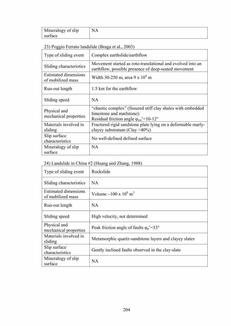
204

Mineralogy of slip surface

NA

23) Poggio Ferrato landslide (Braga et al., 2003)

Type of sliding event Complex earthslide/earthflow

Sliding characteristics Movement started as roto-translational and evolved into an earthflow, possible presence of deep-seated movement

Estimated dimensions of mobilized mass Width 30-250 m, area 9 x 104 m

Run-out length 1.5 km for the earthflow

Sliding speed NA

Physical and mechanical properties

“chaotic complex” (fissured stiff clay shales with embedded limestone and marlstone): Residual friction angle φres’=10-12°

Materials involved in sliding

Fractured rigid sandstone plate lying on a deformable marly-clayey substratum (Clay >40%)

Slip surface characteristics No well-defined defined surface

Mineralogy of slip surface

NA

24) Landslide in China #2 (Huang and Zhang, 1988)

Type of sliding event Rockslide

Sliding characteristics NA

Estimated dimensions of mobilized mass Volume ~100 x 106 m3

Run-out length NA

Sliding speed High velocity, not determined

Physical and mechanical properties Peak friction angle of faults φp’=33°

Materials involved in sliding Metamorphic quartz-sandstone layers and clayey slates

Slip surface characteristics Gently inclined faults observed in the clay-slate

Mineralogy of slip surface NA

205

Extra information

• Evidence of high-speed sliding due to long run-out of such a huge rock mass

• Inferred average temperature on the slip surface: 350 °C

• A mathematical simulation of the landslide mechanism which takes into account the temperature rise is proposed by the authors

25) Edgerton landslide (Cruden et al., 1995)

Type of sliding event Complex

Sliding characteristics Evolution from reactivated, multiple and rapid rockslide to slow earthflow

Estimated dimensions of mobilized mass Volume ~106 m3

Run-out length NA

Sliding speed NA

Physical and mechanical properties

Bentonitic claystone: Natural moisture content=20-24% Liquid limit=100-125% Plasticity index=55-80% Peak shear strength parameters: cp’ =7 kPa φp’= 35° Residual shear strength parameters: c’rs =0 kPa φ’rs= 9°

Materials involved in sliding

Bedrock of marine claystones, siltstones and deltaic sandstones, overlain by till

Slip surface characteristics Bentonitic claystone

Mineralogy of slip surface Dominant mineral in the clay fraction: montmorillonite

26) Madipo landslide (Zhongyou, 1984)

Type of sliding event Translational rockslide

Sliding characteristics The sliding body moved in four consecutive blocks

Estimated dimensions of mobilized mass

Volume ~ 106 m3, thickness ~20 m, length 300 m, width 220 m

Run-out length 240 m in horizontal direction, 60 m in vertical

Sliding speed Max ~28 m/s

206

Physical and mechanical properties

Intact rock mass: cp’=5-20 T/m2 φp’=20-40° Discontinuities where sliding took place: crs’=0.2-2 T/m2 φrs’=3-5°

Materials involved in sliding

Lacustrine semi-rock strata consisting of siltstones, mudstones and shales, total thickness ~200 m

Slip surface characteristics NA

Mineralogy of slip surface NA

Extra information The author proposes “self-lubrication” as an explanation for such a long run-out

27) New Rara landslide (Hasmi and Haq Izhar, 1984)

Type of sliding event Translational landslide

Sliding characteristics NA

Estimated dimensions of mobilized mass Width ~120 m, length ~300 m

Run-out length NA

Sliding speed NA

Physical and mechanical properties

In the slip plane: Liquid limit=36% Plastic limit=22% Plasticity index=14% Peak strength parameters: cp’=12 kPa φp’=29° Residual values: crs’=0 kPa φrs’=18°

Materials involved in sliding Clay with fragments of sandstone, siltstone and claystone

Slip surface characteristics Clayey silt, polished, slickensided, with high plasticity.

Mineralogy of slip surface

20% sand 50% silt 30% clay

28) Ancona landslide (Hegg, 1984)

Type of sliding event Translational landslide

Sliding characteristics NA

207

Estimated dimensions of mobilized mass Max width ~1.7 km, area ~340 ha, thickness=80m.

Run-out length <50 m

Sliding speed NA

Physical and mechanical properties

Marly clay Unit weight γ ~2 g/cm3 Plastic index =20-40% Peak friction angle φp’=21-25° Peak cohesion cp’=0-180 kPa Residual friction angle φrs’=16-19°

Materials involved in sliding

Cover of sandy and silty clay ~10 m thick, followed by Pleistocene deposits of marly-silty clays and carbonate sands, and Pliocene base layers of heavily overconsolidated marly clay

Slip surface characteristics Principally, heavily overconsolidated marly clay

Mineralogy of slip surface

Clay 40-60% CaCO3 30-60%

29) Vajont landslide (Muller, 1964, Tika and Hutchinson, 1999, Muller and Fairhurst, 1968, Hendron and Patton, 1985, Vardoulakis, 2002a.)

Type of sliding event Rockslide

Sliding characteristics Very fast deep-seated rotational sliding

Estimated dimensions of mobilized mass

Volume ~250 x 106 m3, 40-250 m thick, average thickness~120m

Run-out length 450-500 m

Sliding speed 25-30 m/s

Physical and mechanical properties

Clay in the slip plane: Peak friction angle φp’=22° Residual friction angle: static value φrs’ = 8-10°; dynamic value φrd’=6.6° (Tikka and Hutchinson, 1999)

Materials involved in sliding

Rock formations composed mainly of limestone and marly limestone, with clay intercalations

Slip surface characteristics

Approximately circular shape, with slope varying from 30° at rear scarp to 0° at the toe. Silty-clayey material.

Mineralogy of slip surface

Clay ~50%, of which 50% illite-smectite, <5% kaolinite Calcite 40% Quartz <5%

30) Goldau landslide (Erismann, 1979, Thuro et al., 2005, Thuro et al., 2008)

Type of sliding event Rockslide

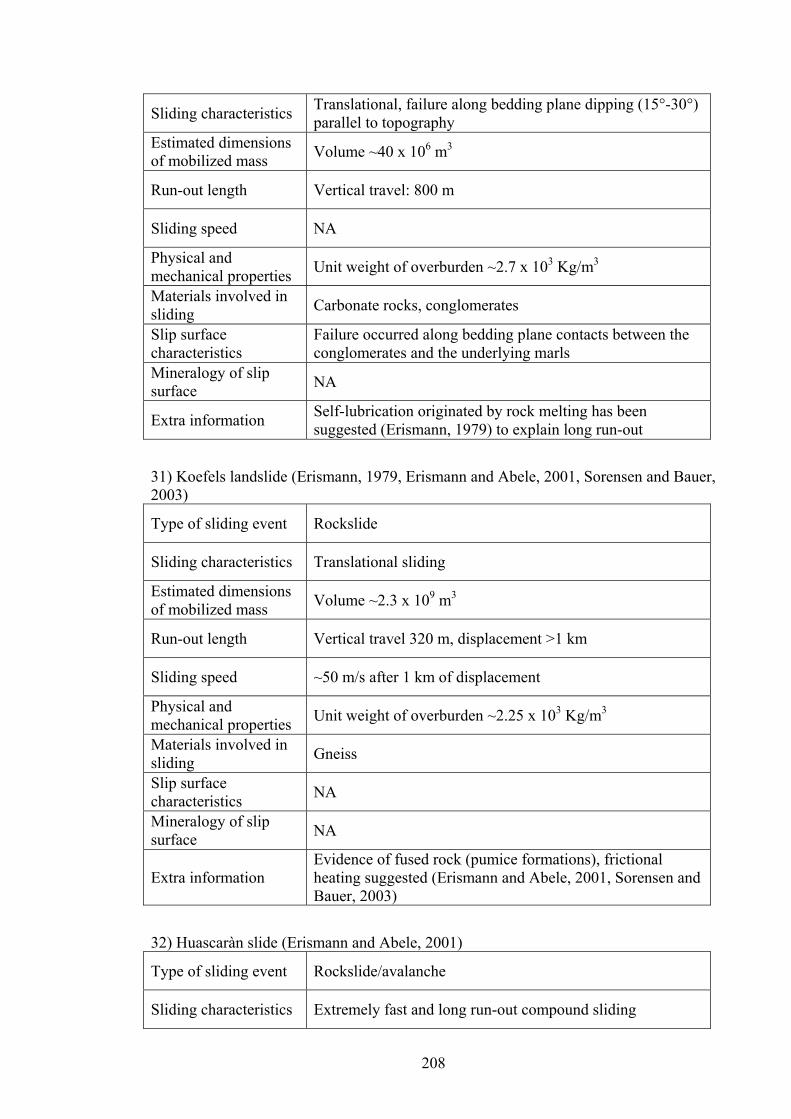
208

Sliding characteristics Translational, failure along bedding plane dipping (15°-30°) parallel to topography

Estimated dimensions of mobilized mass Volume ~40 x 106 m3

Run-out length Vertical travel: 800 m

Sliding speed NA

Physical and mechanical properties Unit weight of overburden ~2.7 x 103 Kg/m3

Materials involved in sliding Carbonate rocks, conglomerates

Slip surface characteristics

Failure occurred along bedding plane contacts between the conglomerates and the underlying marls

Mineralogy of slip surface NA

Extra information Self-lubrication originated by rock melting has been suggested (Erismann, 1979) to explain long run-out

31) Koefels landslide (Erismann, 1979, Erismann and Abele, 2001, Sorensen and Bauer, 2003)

Type of sliding event Rockslide

Sliding characteristics Translational sliding

Estimated dimensions of mobilized mass Volume ~2.3 x 109 m3

Run-out length Vertical travel 320 m, displacement >1 km

Sliding speed ~50 m/s after 1 km of displacement

Physical and mechanical properties Unit weight of overburden ~2.25 x 103 Kg/m3

Materials involved in sliding Gneiss

Slip surface characteristics NA

Mineralogy of slip surface NA

Extra information Evidence of fused rock (pumice formations), frictional heating suggested (Erismann and Abele, 2001, Sorensen and Bauer, 2003)

32) Huascaràn slide (Erismann and Abele, 2001)

Type of sliding event Rockslide/avalanche

Sliding characteristics Extremely fast and long run-out compound sliding

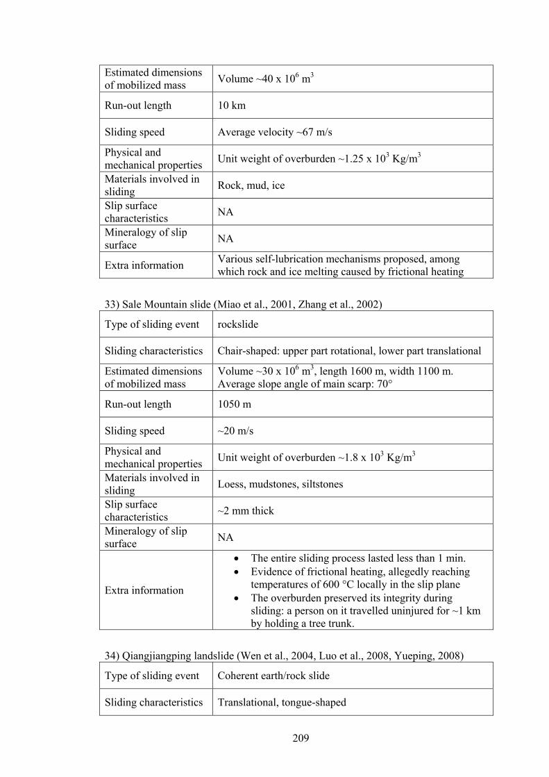
209

Estimated dimensions of mobilized mass Volume ~40 x 106 m3

Run-out length 10 km

Sliding speed Average velocity ~67 m/s

Physical and mechanical properties Unit weight of overburden ~1.25 x 103 Kg/m3

Materials involved in sliding Rock, mud, ice

Slip surface characteristics NA

Mineralogy of slip surface NA

Extra information Various self-lubrication mechanisms proposed, among which rock and ice melting caused by frictional heating

33) Sale Mountain slide (Miao et al., 2001, Zhang et al., 2002)

Type of sliding event rockslide

Sliding characteristics Chair-shaped: upper part rotational, lower part translational

Estimated dimensions of mobilized mass

Volume ~30 x 106 m3, length 1600 m, width 1100 m. Average slope angle of main scarp: 70°

Run-out length 1050 m

Sliding speed ~20 m/s

Physical and mechanical properties Unit weight of overburden ~1.8 x 103 Kg/m3

Materials involved in sliding Loess, mudstones, siltstones

Slip surface characteristics ~2 mm thick

Mineralogy of slip surface NA

Extra information

• The entire sliding process lasted less than 1 min. • Evidence of frictional heating, allegedly reaching

temperatures of 600 °C locally in the slip plane • The overburden preserved its integrity during

sliding: a person on it travelled uninjured for ~1 km by holding a tree trunk.

34) Qiangjiangping landslide (Wen et al., 2004, Luo et al., 2008, Yueping, 2008)

Type of sliding event Coherent earth/rock slide

Sliding characteristics Translational, tongue-shaped

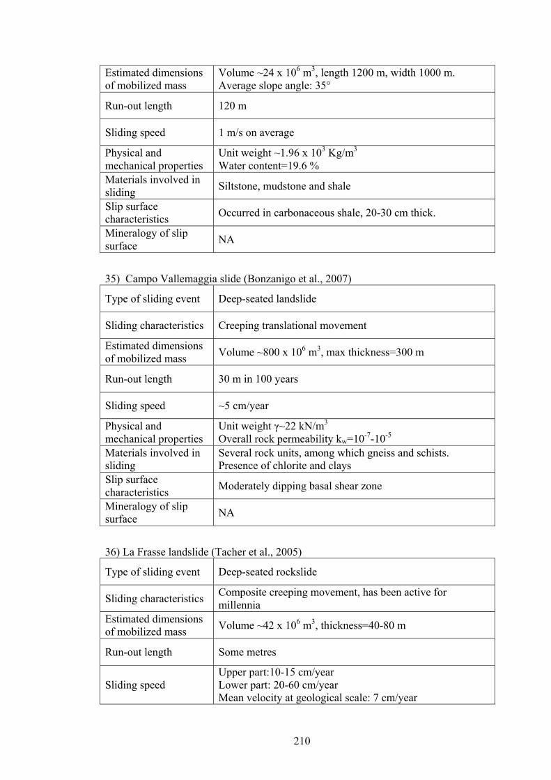
210

Estimated dimensions of mobilized mass

Volume ~24 x 106 m3, length 1200 m, width 1000 m. Average slope angle: 35°

Run-out length 120 m

Sliding speed 1 m/s on average

Physical and mechanical properties

Unit weight ~1.96 x 103 Kg/m3 Water content=19.6 %

Materials involved in sliding Siltstone, mudstone and shale

Slip surface characteristics Occurred in carbonaceous shale, 20-30 cm thick.

Mineralogy of slip surface NA

35) Campo Vallemaggia slide (Bonzanigo et al., 2007)

Type of sliding event Deep-seated landslide

Sliding characteristics Creeping translational movement

Estimated dimensions of mobilized mass Volume ~800 x 106 m3, max thickness=300 m

Run-out length 30 m in 100 years

Sliding speed ~5 cm/year

Physical and mechanical properties

Unit weight γ~22 kN/m3 Overall rock permeability kw=10-7-10-5

Materials involved in sliding

Several rock units, among which gneiss and schists. Presence of chlorite and clays

Slip surface characteristics Moderately dipping basal shear zone

Mineralogy of slip surface NA

36) La Frasse landslide (Tacher et al., 2005)

Type of sliding event Deep-seated rockslide

Sliding characteristics Composite creeping movement, has been active for millennia

Estimated dimensions of mobilized mass Volume ~42 x 106 m3, thickness=40-80 m

Run-out length Some metres

Sliding speed Upper part:10-15 cm/year Lower part: 20-60 cm/year Mean velocity at geological scale: 7 cm/year

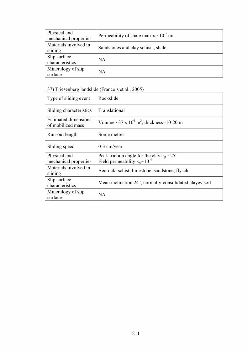
211

Physical and mechanical properties Permeability of shale matrix ~10-7 m/s

Materials involved in sliding Sandstones and clay schists, shale

Slip surface characteristics NA

Mineralogy of slip surface NA

37) Triesenberg landslide (Francois et al., 2005)

Type of sliding event Rockslide

Sliding characteristics Translational

Estimated dimensions of mobilized mass Volume ~37 x 106 m3, thickness=10-20 m

Run-out length Some metres

Sliding speed 0-3 cm/year

Physical and mechanical properties

Peak friction angle for the clay φp’~25° Field permeability kw~10-4

Materials involved in sliding Bedrock: schist, limestone, sandstone, flysch

Slip surface characteristics Mean inclination 24°, normally-consolidated clayey soil

Mineralogy of slip surface NA

212

References

Abramowitz, M. and I. A. Stegun (1964). Handbook of mathematical functions with formulas, graphs, and mathematical tables. Washington, U.S. Govt. Print. Off.

Agliardi, F., G. Crosta, et al. (2001). "Structural constraints on deep-seated slope deformation kinematics." Engineering Geology 59(1-2): 83-102.

Alexandre, J., F. Saboya, et al. (1999). "Photoacoustic thermal characterization of kaolinite clays." Analyst 124(8): 1209-1214.

Anderson, D. L. (1980). An earthquake induced heat mechanism to explain the loss of strength of large rock and earth slides. Proceedings of the International conference on engineering for protection from natural disasters, Bangkok.

Andersson, H., P. E. Bengtsson, et al. (2000). The landslide at Vagnharad in Sweden. Proceedings of the 8th international Symposium on Landslides, Cardiff, Thomas Thelford.

Antoine, P., D. Fabre, et al. (1988). Propriètès gèotechniques de quelques ensembles gèologiques propices aux glissements de terrains. Proceedings of the 5th International Symposium on Landslides, Lausanne.

Azzoni, A., S. Chiesa, et al. (1992). "The Valpola Landslide." Engineering Geology 33(1): 59-70.

Baldi, G., T. Hueckel, et al. (1988). "Thermal Volume Changes of the Mineral Water-System in Low-Porosity Clay Soils." Canadian Geotechnical Journal 25(4): 807-825.

Baldi, G., T. Hueckel, et al. (1991). Developments in modelling of thermo-hydro-geomechanical behaviour of Boom clay and clay-based buffer materials, Report EUR 13365, Commission of the European Communities, Nuclear science and technology.

Bandis, S. C., G. Delmonaco, et al. (1996). Landslide phenomena during the extreme meteorological event of 4-6 November 1994 in the Piemonte Region in N Italy. Proceedings of the 7th International Symposium on Landslides. K. Senneset: 623-628.

Baraza, J., H. J. Lee, et al. (1990). "Geotechnical Characteristics and Slope Stability on the Ebro Margin, Western Mediterranean." Marine Geology 95(3-4): 379-393.

Bell, D. H. and J. R. Pettinga (1988). Bedding-Controlled Landslides in New-Zealand Soft Rock Terrain. Proceedings of the 5th International Symposium on Landslides.

Bentley, S. P. and H. J. Siddle (1996). "Landslide research in the South Wales coalfield." Engineering Geology 43(1): 65-80.

Bojanowski, A. (2007). Als der Berg in den See fiel. Süddeutsche Zeitung 248. Bonzanigo, L., E. Eberhardt, et al. (2007). "Long-term investigation of a deep-seated

creeping landslide in crystalline rock. Part I. Geological and hydromechanical factors controlling the Campo Vallemaggia landslide." Canadian Geotechnical Journal 44(10): 1157-1180.

Booth, J. S., D. W. O'Leary, et al. (1991). U.S. Atlantic continental slope landslides: their distribution, general attributes, and implications. U. S. D. o. t. interior, U.S. Geological Survey.

213

Borja, R. I. and S. R. Lee (1990). "Cam Clay Plasticity .1. Implicit Integration of Elastoplastic Constitutive Relations." Computer Methods in Applied Mechanics and Engineering 78(1): 49-72.

Braga, G., C. Messina, et al. (2003). Study of a complex landslide movement for risk assessment: the example of the poggio ferrato landslide (northern Italy). Proc. International Conference on Fast Slope Movements: Prediction and Prevention for Risk Mitigation. Napoli, AGI.

Buccolini, M. and N. Sciarra (1996). The Caramanico Landslide (Abruzzo, Italy). Seventh International Symposium on Landslides, Trondheim, Balkema.

Bugge, T., R. H. Belderson, et al. (1988). "The Storegga Slide." Philosophical Transactions of the Royal Society of London Series a-Mathematical Physical and Engineering Sciences 325(1586): 357-&.

Campanella, R. G., J. K. Mitchell, et al. (1968). Influence of temperature variations on soil behavior. Berkeley, University of California, Institute of Transportation and Traffic Engineering, Soil Mechanics and Bituminous Materials Research Laboratory.

Canals, M., G. Lastras, et al. (2004). "Slope failure dynamics and impacts from seafloor and shallow sub-seafloor geophysical data: case studies from the COSTA project." Marine Geology 213(1-4): 9-72.

Cappa, F., Y. Guglielmi, et al. (2004). "Hydromechanical modeling of a large moving rock slope inferred from slope levelling coupled to spring long-term hydrochemical monitoring: Example of the La Clapie're landslide (Southern Alps, France)." Journal of Hydrology 291(1-2): 67-90.

Catalano, A., V. Chieppa, et al. (2000). Interacion between dams and landslides: three case histories. 8th int. Symposium on Landslides, Cardiff, Thomas Thelford.

Chang, K. J., A. Taboada, et al. (2005a). "Analysis of landsliding by earthquake shaking using a block-on-slope thermo-mechanical model: Example of Jiufengershan landslide, central Taiwan." Engineering Geology 80(1-2): 151-163.

Chang, K. J., A. Taboada, et al. (2005b). "Geological and morphological study of the Jiufengershan landslide triggered by the Chi-Chi Taiwan earthquake." Geomorphology 71(3-4): 293-309.

Chihara, K., S. Iwanaga, et al. (1994). "Geohistorical Development of the Tochiyama Landslide in North-Central Japan." Engineering Geology 38(3-4): 205-219.

Cornforth, D. H. and J. A. Lowell (1996). The 1994 submarine slope failure at Skagway, Alaska. Seventh International Symposium on Landslides, Trondheim, Balkema.

Corominas, J. (1996). "The angle of reach as a mobility index for small and large landslides." Canadian Geotechnical Journal 33(2): 260-271.

Crosta, G. B. and F. Agliardi (2002). "How to obtain alert velocity thresholds for large rockslides." Physics and Chemistry of the Earth 27(36): 1557-1565.

Crosta, G. B., H. Chen, et al. (2004). "Replay of the 1987 Val Pola Landslide, Italian Alps." Geomorphology 60(1-2): 127-146.

Crosta, G. B., S. Imposimato, et al. (2005). "Small fast-moving flow-like landslides in volcanic deposits: The 2001 Las Colinas Landslide (El Salvador)." Engineering Geology 79(3-4): 185-214.

Cruden, D. M., Z. Y. Lu, et al. (1997). "The 1939 Montagneuse River landslide, Alberta." Canadian Geotechnical Journal 34(5): 799-810.

Cruden, D. M., S. Thomson, et al. (1995). "The Edgerton landslides." Canadian Geotechnical Journal 32(6): 989-1001.

Cui, Y. J., N. Sultan, et al. (2000). "A thermomechanical model for saturated clays." Canadian Geotechnical Journal 37(3): 607-620.

214

De Blasio, F. V. and A. Elverhoi (2008). "A model for frictional melt production beneath large rock avalanches." Journal of Geophysical Research-Earth Surface 113(F2).

Delage, P., N. Sultan, et al. (2000). "On the thermal consolidation of Boom clay." Canadian Geotechnical Journal 37(2): 343-354.

Demars, K. R. and R. D. Charles (1982). "Soil Volume Changes Induced by Temperature Cycling." Canadian Geotechnical Journal 19(2): 188-194.

Demers, D. and D. Robitaille (2000). The St. Boniface landslide of April 1996: A large retrogressive landslide in sensitive clay with little flow component. Proceedings of the 8th international Symposium on Landslides, Cardiff, Thomas Thelford.

Desgagnes, P., J. Locat, et al. (2000). Geotechnical properties of a mass flow deposit on the Hudson Apron, off New Jersey, U.S.A. 53rd Canadian Geotechnical Conference, Montreal.

Despax, D. (1976). Etude de l'influence de la temperature sur les proprietés des argiles saturées. Thése de doctorat. Grenoble, Université de Grenoble.

Dowell, M. and P. Jarratt (1972). "The “Pegasus” method for computing the root of an equation." BIT Numerical Mathematics 12(4): 503-508.

Erismann, T. H. (1979). "Mechanisms of Large Landslides." Rock Mechanics 12: 15-46.

Erismann, T. H. and G. Abele (2001). Dynamics of Rockslides and Rockfalls. Berlin Heidelberg, Springer-Verlag.

Evans, S. G. and J. V. DeGraff (2002). Catastrophic landslides : effects, occurrence, and mechanisms. Boulder, CO, Geological Society of America.

Favaretti, M., P. Previatello, et al. (1996). A case history of a translational landslide in the Chiampo Valley (Italy). Proceedings of the 7th International Symposium on Landslides. K. Senneset: 1219-1224.

Fleming, R. W., S. D. Ellen, et al. (1989). "Transformation of Dilative and Contractive Landslide Debris into Debris Flows - an Example from Marin County, California." Engineering Geology 27(1-4): 201-223.

Follacci, J. P., P. Guardia, et al. (1988). Geodynamic framework of La Clapière landslide (Maritime Alps, France). Proceedings of the 5th International Symposium on Landslides, Lausanne.

Forsberg, C. F. and J. Locat (2005). "Mineralogical and microstructural development of the sediments on the Mid-Norwegian margin." Marine and Petroleum Geology 22(1-2): 109-122.

Francois, B., L. Tacher, et al. (2007). "Numerical modelling of the hydrogeological and geomechanical behaviour of a large slope movement: the Triesenberg landslide (Liechtenstein)." Canadian Geotechnical Journal 44: 840-857.

Gaziev, E. (1984). Study of the Usoy landslide in Pamir. IV International Symposium on Landslides Toronto.

Ghabezloo, S. and J. Sulem (2008). "Stress dependent thermal pressurization of a fluid-saturated rock." Rock Mechanics and Rock Engineering.

Gokceoglu, C., H. Sonmez, et al. (2005). "The 17 March 2005 Kuzulu landslide (Sivas, Turkey) and landslide-susceptibility map of its near vicinity." Engineering Geology 81(1): 65-83.

Griffiths, J. S., J. N. Hutchinson, et al. (2004). "The reactivation of a landslide during the construction of the Ok Ma tailings dam, Papua New Guinea." Quarterly Journal of Engineering Geology and Hydrogeology 37: 173-186.

Guadagno, F. M. and S. Perriello Zampelli (2000). Triggering mechanisms of the Landslides that inundated Sarno, Quindici, Siano, and Bracigliano (S. Italy) on

215

May 5-6, 1998. Proceedings of the 8th international Symposium on Landslides, Cardiff, Thomas Thelford.

Guzzetti, F. (2000). "Landslide fatalities and the evaluation of landslide risk in Italy." Engineering Geology 58(2): 89-107.

Guzzetti, F., C. P. Stark, et al. (2005). "Evaluation of flood and landslide risk to the population of Italy." Environmental Management 36(1): 15-36.

Habib, P. (1975). "Production of gaseous pore pressure during rock slides." Rock Mechanics and Rock Engineering 7(4): 193-197.

Habibagahi, K. (1977). "Temperature effect and the concept of effective void ratio." Indian Geotechnical Journal 1: 14-34.

Hampton, M. A., H. J. Lee, et al. (1996). "Submarine landslides." Reviews of Geophysics 34(1): 33-59.

Hegg, U. (1984). Case history of a large coastal landslide in pliocene clays. Proc. IV International Symposium on Landslides Toronto.

Helmstetter, A., D. Sornette, et al. (2004). "Slider block friction model for landslides: Application to Vaiont and La Clapiere landslides." Journal of Geophysical Research-Solid Earth 109(B2).

Hendron, A. J. and F. D. Patton (1985). The Vaiont slide, a geotehnical analysis based on new geologic observations of the failure surface. Technical Report GL-85-5. Washington, DC, Department of the Army US Corps of Engineers.

Hendron, A. J. and F. D. Patton (1987). "The Vaiont Slide - a Geotechnical Analysis Based on New Geologic Observations of the Failure Surface." Engineering Geology 24(1-4): 475-491.

Hicher, P. Y. (1974). Etude des proprietés mechaniques des argiles à l'aide d'essais triaxiaux, influence de la vitesse et de la temperature. Report of the soil mechanics laboratory. Paris, Ecole Centrale de Paris.

Hoffman, J. D. (2001). Numerical methods for engineers and scientists. New York Marcel Dekker.

Huang, C. C., Y. H. Lee, et al. (2001). "Influence of surface-normal ground acceleration on the initiation of the Jih-Feng-Erh-Shan landslide during the 1999 Chi-Chi, Taiwan, earthquake." Bulletin of the Seismological Society of America 91(5): 953-958.

Huang, R. Q. and S. T. Wang (1988). Rolling Friction Mechanism for the High-Speed Motion of a Large-Scale Landslide. Proceedings of the 5th International Symposium on Landslides. C. Bonnard: 187-191.

Huang, R. Q. and Z. Y. Zhang (1988). Analysis and Mathematical Simulation of a Large Landslide Formed by Composite Mechanism. Proceedings of the 5th International Symposium on Landslides. C. Bonnard: 673-678.

Hueckel, T. and G. Baldi (1990). "Thermoplasticity of Saturated Clays - Experimental Constitutive Study." Journal of Geotechnical Engineering-Asce 116(12): 1778-1796.

Hueckel, T. and M. Borsetto (1990). "Thermoplasticity of Saturated Soils and Shales - Constitutive-Equations." Journal of Geotechnical Engineering-Asce 116(12): 1765-1777.

Hueckel, T. and A. Peano (1987). "Some geotechnical aspects of radioactive waste isolation in continental clays." Computers and Geotechnics 3: 157-182.

Hueckel, T. and R. Pellegrini (1989). Modelling of thermal failure of saturated clays. Proceedings of Numerical Models in Geomechanics, Elsevier.

Hueckel, T. and R. Pellegrini (1991). "Thermoplastic modelling of undrained failure of saturated clay due to heating." Soils and Foundations 31(3): 1-16.

216

Huhnerbach, V. and D. G. Masson (2004). "Landslides in the North Atlantic and its adjacent seas: an analysis of their morphology, setting and behaviour." Marine Geology 213(1-4): 343-362.

Hunter, G. J. and R. Fell (2003). Mechanics of failure of soil slopes leading to "rapid" failure. Proc. International Conference on Fast Slope Movements: Prediction and Prevention for Risk Mitigation Napoli, AGI.

Hurlimann, M., A. Ledesma, et al. (1999). "Conditions favouring catastrophic landslides on Tenerife (Canary Islands)." Terra Nova 11(2-3): 106-111.

Hutchinson, J. N. (1961). "A landslide on a thin layer of quick clay at Furre, Central Norway." Géotechnique 11: 69–94.

Hutchinson, J. N. (1988). Morphological and Geotechnical parameters of Landslides in relation to Geology and Hydrogeology. V Intl Symposium on Landslides, Lausanne.

IUGS - International working group, L. (1995). "A suggested method for describing the rate of movement of a landslide." Bullettin of the International Association of Engineering Geology 52: 75-78.

Kilburn, C. R. J. and D. N. Petley (2003). "Forecasting giant, catastrophic slope collapse: lessons from Vajont, Northern Italy." Geomorphology 54(1-2): 21-32.

Koiter, W. T. (1960). General theorems for elastic-plastic solids. Progress in solid mechanics. I. N. S. a. R. Hill. Amsterdam: 167-221.

Kvalstad, T. J., L. Andresen, et al. (2005a). "The Storegga slide: evaluation of triggering sources and slide mechanics." Marine and Petroleum Geology 22(1-2): 245-256.

Kvalstad, T. J., F. Nadim, et al. (2005b). "Soil conditions and slope stability in the Ormen Lange area." Marine and Petroleum Geology 22(1-2): 299-310.

Laloui, L. (2001). "Thermo-mechanical behaviour of soils." Environmental geomechanics 5: 809-843.

Laloui, L. and C. Cekerevac (2003). "Thermo-plasticity of clays: An isotropic yield mechanism." Computers and Geotechnics 30(8): 649-660.

Laloui, L., C. Cekerevac, et al. (2005). "Constitutive modelling of the thermo-plastic behaviour of soils." Revue Europeenne de genie civil 9(5-6): 635-650.

Laloui, L., C. Cekerevac, et al. (2002). Thermo-plasticity of clays: a simple constitutive approach. Environmental geomechanics - Monte Verita` 2002. L.Vulliet.

Lee, E. M., D. K. C. Jones, et al. (2000). The landslide environment of Great Britain. Proceedings of the 8th international Symposium on Landslides

Cardiff, Thomas Thelford. Lee, H. J., W. C. Schwab, et al. (1991). Submarine Landslides: an introduction. U. S. D.

o. t. interior, U.S. Geological Survey. Legros, F. (2002). "The mobility of long-runout landslides." Engineering Geology 63(3-

4): 301-331. Legros, F., J. M. Cantagrel, et al. (2000). "Pseudotachylyte (frictionite) at the base of

the Arequipa volcanic landslide deposit (Peru): Implications for emplacement mechanisms." Journal of Geology 108(5): 601-611.

Lehane, B. M. and R. J. Jardine (1992). "Residual Strength Characteristics of Bothkennar Clay." Geotechnique 42(2): 363-367.

Leroueil, S., J. Locat, et al. (1996). Geotechnical characterization of slope movements. Proceedings of the 7th International Symposium on Landslides. K. Senneset: 53-74.

Lin, A. M., A. L. Chen, et al. (2001). "Frictional fusion due to coseismic landsliding during the 1999 Chi-Chi (Taiwan) M-L 7.3 earthquake." Geophysical Research Letters 28: 4011-4014.

217

Locat, J. and H. J. Lee (2000). Submarine Landslides: Advances and Challenges. 8th int. Symposium on Landslides, Cardiff, Thomas Thelford.

Luo, X., A. Che, et al. (2008). Failure mechanism of slipping zone soil of the Qiangjiangping landslide in the Three Gorges reservoir area: A study based on Dead Load test. Proceedings of the 10th International Symposium on Landslides and Engineered Slopes, Xi'An, China, Taylor and Francis.

Lykousis, V., G. Roussakis, et al. (2002). "Sliding and regional slope stability in active margins: North Aegean Trough (Mediterranean)." Marine Geology 186(3-4): 281-298.

Mandel, J. (1965). "Une generalisation de la theorie de Koiter." International Journal of Solid Structures 1: 273-295.

Marques, M. E. S., S. Leroueil, et al. (2004). "Viscous behaviour of St-Roch-de-l'Achigan clay, Quebec." Canadian Geotechnical Journal 41(1): 25-38.

Martinez, J. F., J. Cartwright, et al. (2005). "3D seismic interpretation of slump complexes: examples from the continental margin of Israel." Basin Research 17(1): 83-108.

Masch, L., H. R. Wenk, et al. (1985). "Electron-Microscopy Study of Hyalomylonites - Evidence for Frictional Melting in Landslides." Tectonophysics 115(1-2): 131-160.

Mase, G. E. (1970). Schaum's outline of theory and problems of continuum mechanics. New York, McGraw-Hill.

Modaressi, H. and L. Laloui (1997). "A thermo-viscoplastic constitutive model for clays." International Journal for Numerical and Analytical Methods in Geomechanics 21(5): 313-335.

Morgenstern, N. R. and J. S. Tschalenko (1967). "Microscopic structures in kaolin subjected to direct shear." Géotechnique 17(4): 309-328.

Muir Wood, D. (1990). Soil behaviour and critical state soil mechanics, Cambridge university press.

Muller, L. (1964). "The rock slide in the Vaiont valley." Felsmech. Ingenieurgeol. 2: 148-212.

Muller, L. and C. Fairhurst (1968). "New Considerations on the Vaiont Slide " Rock Mech Eng Geol VI(1-2).

NIST/SEMATECH. (2003, 18/07/2006). "e-Handbook of Statistical Methods." from http://www.itl.nist.gov/div898/handbook/.

Okura, Y., H. Kitahara, et al. (2003). "Topography and volume effects on travel distance of surface failure." Engineering Geology 67(3-4): 243-254.

Oyagi, N., M. Sorriso-Valvo, et al. (1994). "Introduction to the Special Issue of the Symposium on Deep-Seated Landslides and Large-Scale Rock Avalanches." Engineering Geology 38(3-4): 187-188.

Pastor, M., O. C. Zienkiewicz, et al. (1990). "Generalized Plasticity and the Modeling of Soil Behavior." International Journal for Numerical and Analytical Methods in Geomechanics 14(3): 151-190.

Peace, G. S. (1993). Taguchi methods : a hands-on approach. Reading, Mass., Addison-Wesley.

Petley, D. N. and R. J. Allison (1997). "The mechanics of deep-seated landslides." Earth Surface Processes and Landforms 22(8): 747-758.

Polloni, G., P. Aleotti, et al. (1996). Heavy rain triggered landslides in the Piemonte region (Italy). Proceedings of the 7th International Symposium on Landslides. K. Senneset. Trondheim, Balkema: 1955-1960.

Potts, D. M. and L. Zdravkovic (1999). Finite element analysis in geotechnical engineering : theory. London; Reston, VA, Telford ; Distributed by ASCE Press.

218

Powrie, W. (1997). Soil mechanics : concepts and applications. London; New York, E & FN Spon.

Prager, W. (1958). "Non-isothermal plastic deformation." Bol. Konike Nederl. Acad. Wet. 8(61/3): 176-182.

Press, W. H., B. P. Flannery, et al. (1988). Numerical recipes in C : the art of scientific computing. Cambridge [Cambridgeshire]; New York, Cambridge University Press. Prior, D. (1988). Subaqueous Landslides. Proceedings of the 5th International

Symposium on Landslides. Puzrin, A. M. and L. N. Germanovich (2005). "The growth of shear bands in the

catastrophic failure of soils." Proceedings of the Royal Society a-Mathematical Physical and Engineering Sciences 461(2056): 1199-1228.

Rice, J. R. (2006). "Heating and weakening of faults during earthquake slip." Journal of Geophysical Research-Part B-Solid Earth 111(B5): 29 pp.-29 pp.

Roberts, J. A. and A. Cramp (1996). "Sediment stability on the western flanks of the Canary Islands." Marine Geology 134(1-2): 13-30.

Robinet, J. C., A. Rahbaoui, et al. (1996). "A constitutive thermomechanical model for saturated clays." Engineering Geology 41(1-4): 145-169.

Roscoe, K. and J. Burland (1968). On generalized stress strain behaviour of wet clay, Cambridge University Press.

Roscoe, K. and A. N. Schofield (1963). Mechanical behaviour of an idealised 'wet' clay. Proc. European Conf. on soil Mechanics and Foundation Engineering, Wiesbaden.

Sangrey, D. A. (1977). "Marine Geotechnology - State of the Art." Marine Geotechnology 2: 45-80.

Schofield, A. N. and C. P. Wroth (1968). Critical State Soil Mechanics. London, McGraw Hill.

Schrefler, B. (2005). "Finite element analysis of strain localization in multiphase materials." from http://alert.epfl.ch/Archive/ALERT2005/s/slides/Schrefler_aussois2005-localization-sent.pdf.

Shou, K. J. and C. F. Wang (2003). "Analysis of the Chiufengershan landslide triggered by the 1999 Chi-Chi earthquake in Taiwan." Engineering Geology 68(3-4): 237-250.

Shreve, R. L. (1966). "Sherman Landslide, Alaska." Science, new series 154(3757): 1639-1643.

Shuzui, H. (2000). Landslide classification based on the Properties of Slip Surface. 8th int. Symposium on Landslides, Cardiff, Thomas Thelford.

Silva, A. J., C. D. P. Baxter, et al. (2004). "Investigation of mass wasting on the continental slope and rise." Marine Geology 203(3-4): 355-366.

Skempton, A. W. (1985). "Residual Strength of Clays in Landslides, Folded Strata and the Laboratory." Geotechnique 35(1): 3-18.

Sloan, S. W., A. J. Abbo, et al. (2001). "Refined explicit integration of elastoplastic models with automatic error control." Engineering Computations 18(1-2): 121-154.

Sørensen, S.-A. and B. Bauer (2003). "On the dynamics of the Köfels sturzstrom." Geomorphology 54(1-2): 11-19.

Sornette, D., A. Helmstetter, et al. (2004). "Towards landslide predictions: two case studies." Physica a-Statistical Mechanics and Its Applications 338(3-4): 605-632.

219

Stead, D. (2003). "Dynamics of Rockslides and Rockfalls - T.H. Erismann and G. Abele. Springer-Verlag Berlin Heidelberg, 2001. 316 pages. ISBN 3-540-67198-6. Hardbound." Engineering geology. 66(3): 320.

Strom, A. L. (1996). Some morphological types of long-runout rockslides: Effect of the relief on their mechanism and on the rockslide deposits distribution. Seventh International Symposium on Landslides, Trondheim, Balkema.

Sulem, J., P. Lazar, et al. (2007). "Thermo-poro-mechanical properties of clayey gouge and application to rapid fault shearing." International Journal for Numerical and Analytical Methods in Geomechanics 31(3): 523-540.

Sulem, J., I. Vardoulakis, et al. (2004). "Experimental characterization of the thermo-poro-mechanical properties of the Aegion Fault gouge." Comptes Rendus Geoscience 336(4-5): 455-466.

Sulem, J., I. Vardoulakis, et al. (2005). "Thermo-poro-mechanical properties of the Aigion fault clayey gouge - Application to the analysis of shear heating and fluid pressurization." Soils and Foundations 45(2): 97-108.

Sultan, N. (1997). Etude du comportement thermo-mèchanique de l'argile de Boom: expériences et modélisation. Thèse de doctorat. ENPC. Paris, CERMES.

Sultan, N., P. Delage, et al. (2001). Temperature effects on the volume change behaviour of Boom clay. Workshop on Key Issues in Waste Isolation Research, Barcelona, Spain, Elsevier Science Bv.

Sultan, N., P. Delage, et al. (2002). "Temperature effects on the volume change behaviour of Boom clay." Engineering Geology 64(2-3): 135-145.

Tacher, L., C. Bonnard, et al. (2005). "Modelling the behaviour of a large landslide with respect to hydrogeological and geomechanical parameter heterogeneity." Landslides 2(1): 3-14.

Taguchi, G. and O. Asian Productivity (1986). Introduction to quality engineering; designing quality into products and processes. White Plains, N.Y.; Dearborn, Mich., Unipub/Quality Resources; American Supplier Institute.

Taguchi, G., M. El Sayed, et al. (1989). Quality Engineering and quality systems. New York, McGraw-Hill.

Tarchi, D., N. Casagli, et al. (2003). "Landslide monitoring by using ground-based SAR interferometry: an example of application to the Tessina landslide in Italy." Engineering Geology 68(1-2): 15-30.

Taylor, D. W. (1948). Fundamentals of soil mechanics. New York, J. Wiley. Thuro, K., C. Berner, et al. (2005). Der Bergsturz von Goldau 1806 -

Versagensmechanismen in wechsellagernden Konglomeraten und Mergeln. Veroffentlichungen von der 15. Tagung fur Ingenieurgeologie : Erlangen, 06. - 09. April 2005 ; ( Proceedings of the 15th Conference on Engineering Geology), Erlangen.

Tika, T. E. and J. N. Hutchinson (1999). "Ring shear tests on soil from the Vaiont landslide slip surface." Geotechnique 49(1): 59-74.

Tinti, S., F. Zaniboni, et al. (2007). Tsunamigenic landslides in the western Corinth Gulf: Numerical scenarios. 3rd International Symposium on Submarine Mass Movements and Their Consequences, Santorini, GREECE, Springer.

Towhata, I., P. Kuntiwattanakul, et al. (1995). "Discussion on volume change of clays induced by heating as observed in consolidation tests (Towhata and al. 1993)." Soils and Foundations 35(3): 124-127.

Troncone, A. (2005). "Numerical analysis of a landslide in soils with strain-softening behaviour." Geotechnique 55(8): 585-596.

220

Turrini, M. C., F. Fiorani, et al. (1996). Analysis of a landslide in a complex formation. Proceedings of the 7th International Symposium on Landslides. K. Senneset: 913-918.

Urgeles, R., D. Leynaud, et al. (2006). "Back-analysis and failure mechanisms of a large submarine slide on the ebro slope, NW Mediterranean." Marine Geology 226(3-4): 185-206.

Van Beek, L. P. H. and T. W. J. Van Asch (1996). The mobility characteristics of the Valette landslide. Seventh International Symposium on Landslides, Trondheim, Balkema.

Van Genuchten, P. M. B. (1988). Intermittent sliding of a landslide in varved clays. Proceedings of the 5th International Symposium on Landslides, Lausanne.

Vardoulakis, I. (2000). "Catastrophic landslides due to frictional heating of the failure plane." Mechanics of Cohesive-Frictional Materials 5(6): 443-467.

Vardoulakis, I. (2001). Thermo-poro-mechanical analysis of rapid fault deformation. International Conference on Micromechanics of Granular Media, Sendai, Japan, Rotterdam: Balkema.

Vardoulakis, I. (2002a). "Dynamic thermo-poro-mechanical analysis of catastrophic landslides." Geotechnique 52(3): 157-171.

Vardoulakis, I. (2002b). "Steady shear and thermal run-away in clayey gouges." International Journal of Solids and Structures 39(13-14): 3831-3844.

Vardoulakis, I. (2003). "Dynamic thermo-poro-mechanical analysis of catastrophic landslides." Geotechnique 53(5): 523-524.

Vardoulakis, I. and J. Sulem (1995). Bifurcation analysis in Geomechanics. Glasgow, Chapman & Hall.

Varnes, D. J. (1978). "Slope movement types and processes." Special report, Washington D.C.: Transportation research board, National Academy of sciences(176): 11-33.

Veveakis, E., I. Vardoulakis, et al. (2007). "Thermoporomechanics of creeping landslides: The 1963 Vaiont slide, northern Italy." Journal of Geophysical Research-Earth Surface 112(F3).

Voight, B. and C. Faust (1982). "Frictional Heat and Strength Loss in Some Rapid Landslides." Geotechnique 32(1): 43-54.

Voight, B. and C. Faust (1992). "Frictional Heat and Strength Loss in Some Rapid Landslides - Error Correction and Affirmation of Mechanism for the Vaiont Landslide." Geotechnique 42(4): 641-643.

Wang, W. N., M. Chigira, et al. (2003). "Geological and geomorphological precursors of the Chiu-fen-erh-shan landslide triggered by the Chi-chi earthquake in central Taiwan." Engineering Geology 69(1-2): 1-13.

Wen, B., S. Wang, et al. (2004). "Characteristics of rapid giant landslides in China." Landslides 1(4): 247-261.

Whalley, W. B., G. R. Douglas, et al. (1983). "The Magnitude and Frequency of Large Rockslides in Iceland in the Post-Glacial." Geografiska Annaler Series a-Physical Geography 65(1-2): 99-110.

Wibberley, C. A. J. and T. Shimamoto (2005). "Earthquake slip weakening and asperities explained by thermal pressurization." Nature 436(7051): 689-692.

Wieczorek, G. F., M. Jakob, et al. (2003). Preliminary assessment of landslide-induced wave hazards: Tidal Inlet, Glacier Bay National Park, Alaska, U. S. Geological Survey Open-File Report 03-100.

Wilson, A. J., W. Murphy, et al. (2000). Some obsevations on the Geotechnics and movement of Large Volume Earth Flows in Alpine Regions. Proceedings of the 8th international Symposium on Landslides, Cardiff, Thomas Thelford.

221

Yueping, Y. (2008). Landslides in China - Selected case studies. Beijing, China Land Press.

Zhang, Z. Y., S. M. Chen, et al. (2002). 1983 Sale Mountain landslide, Gansu Province, China. Catastrophic Landslides: Effects, Occurrence, and Mechanisms. J. V. D. Stephen G. Evans: 149-163.

Zhongyou, L. (1984). Examples of rapid landslides in semi-rock strata. IV International Symposium on Landslides Toronto.

Zhou, Y. (2000). Research and treatment of Shazou Landslide, Sichuan. Proceedings of the 8th international Symposium on Landslides, Cardiff, Thomas Thelford.