1 / 20

Cooling rate of water Group 5: Xihui Yuan, Wenjing Song, Ming Zhong,

Kaiyue Chen, Yue Zhao, Xiangxie Li

目录 1. Abstract: .............................................................................................................................. 1

2. Introduction: ...................................................................................................................... 2

2.1. Statement of the problem: ................................................................................... 2

2.2 objectives: ................................................................................................................. 2

2.3. Rationale .................................................................................................................. 2

3. Literature review ............................................................................................................... 2

3.1. Basic Concept .......................................................................................................... 3

3.2 Existing experiment on the cooling rate of water ........................................... 3

3.3.Predictive conclusions ........................................................................................... 4

4. Methods ............................................................................................................................... 4

4.1. Experiment variables ............................................................................................. 4

4.3. Design of experiment ............................................................................................ 7

4.4. Instrument ............................................................................................................... 8

4.5. Performing the experiment .................................................................................. 9

5. Analysis ............................................................................................................................. 10

5.1. Data analysis ......................................................................................................... 10

5.2. Conclusion ............................................................................................................. 18

6. In-depth research ............................................................................................................ 19

7. Future extension ............................................................................................................. 19

8. Reference .......................................................................................................................... 20

1. Abstract:

This thesis aims at exploring factors that can affect the cooling rate of water.

Water is the foundation of life; however, although we are very familiar with it, it

still has many aspects that we do not quite understand. There are some existing

theories and experiments about this topic, on this basis, we will do further study

to find cooling rate under different conditions. In order to explore the effectors

that have an influence on the cooling condition, we find out different variables,

and select proper ones to be considered in our experiment according to the scope

of our research. Some 2 level factors, factorial designs will be undertaken, and

several analytical methods will be applied to the data got from experiments, until

we get to the ultimate goal and get acquaintance of the cooling procedure.

2 / 20

2. Introduction:

2.1. Statement of the problem:

Water is one of the most common things in our daily life. Nearly all the

students take a bottle of water or hot drink with them every day. Naturally, how to

keep their drink warm in the winter and make hot drink cool as quick as possible

becomes a question that many will concern. But at the same time, few of them

have put their thoughts into action. As a result, this area of knowledge for most

people remains to be relatively blank.

2.2 objectives:

In this experiment, we will measure the cooling rate of different drinks in

different environment, to draw one or more conclusions about better ways of

keeping drink warm in winter and cooling water quickly in summer.

2.3. Rationale

Our experiment is focused on cooling rate of different drinks. As cooling rate

will be relatively certain and stable under certain conditions, so the data will be

meaningful and we can certainly draw some conclusions from it. Different factors

of environment conditions, holding bottles and initial temperature will be

considered. The cooling rate will be measured by thermometer, guaranteeing the

correctness and accuracy of the experiments.

This experiment is focused on water or drink’s cooling in our daily life, so the

experiment subjects will be the most commonly and easily found drink in our life.

And the variables of experiment environment will be designed within the

limitation of real life as well.

3. Literature review

To get some predictive conclusions before the experiment is a very important

method to give us some intuition to estimate whether the experiment is

performing correctly and whether there are some significant wrong message in

the final result. In order to get some intuition and predictive conclusion before the

experiment, we find some literature related to our experiment and do some

forecasts before we do the experiment.

3 / 20

3.1. Basic Concept

There are some very important formulas related closely to our cooling rate

experiment.

Heat conduction formular: 𝑄 = 𝑐𝑚∆𝑇

𝑄 = 𝑡ℎ𝑒 𝑞𝑢𝑎𝑛𝑡𝑖𝑡𝑦 𝑜𝑓 ℎ𝑒𝑎𝑡 𝑐 = 𝑡ℎ𝑒 𝑠𝑝𝑒𝑐𝑖𝑓𝑖𝑐 ℎ𝑒𝑎𝑡 𝑐𝑎𝑝𝑎𝑐𝑖𝑡𝑦 𝑚 = 𝑡ℎ𝑒 𝑞𝑢𝑎𝑛𝑡𝑖𝑡𝑦 𝑜𝑓 𝑡ℎ𝑒 𝑙𝑖𝑞𝑢𝑖𝑑 ∆𝑇 = 𝑡ℎ𝑒 𝑑𝑖𝑓𝑓𝑒𝑟𝑒𝑛𝑐𝑒 𝑏𝑒𝑡𝑤𝑒𝑒𝑛 𝑡ℎ𝑒 𝑖𝑛𝑖𝑡𝑖𝑎𝑙 𝑡𝑒𝑚𝑝𝑒𝑟𝑎𝑡𝑢𝑟𝑒 𝑎𝑛𝑑 𝑡ℎ𝑒 𝑓𝑖𝑛𝑎𝑙 𝑡𝑒𝑚𝑝𝑒𝑟𝑎𝑡𝑢𝑟𝑒

Newton's law of cooling 𝑄 = 𝑞 × 𝑠 × 𝑡

𝑞 = 𝛾 ×𝑇0 − 𝑇1

𝑑

𝛾 = 𝑎 𝑐𝑜𝑛𝑠𝑡𝑎𝑛𝑡 𝑟𝑒𝑙𝑎𝑡𝑒𝑑 𝑡𝑜 𝑡ℎ𝑒 𝑡𝑒𝑥𝑡𝑢𝑟𝑒 𝑜𝑓 𝑡ℎ𝑒 𝑐𝑜𝑛𝑡𝑎𝑖𝑛𝑒𝑟 𝑇0 = 𝑡ℎ𝑒 𝑖𝑛𝑖𝑡𝑖𝑎𝑙 𝑡𝑒𝑚𝑝𝑒𝑟𝑎𝑡𝑢𝑟𝑒 𝑜𝑓 𝑡ℎ𝑒 𝑙𝑖𝑞𝑢𝑖𝑑

𝑇1 = 𝑡ℎ𝑒 𝑡𝑒𝑚𝑝𝑒𝑟𝑎𝑡𝑢𝑟𝑒 𝑜𝑓 𝑡ℎ𝑒 𝑒𝑛𝑣𝑖𝑟𝑜𝑛𝑚𝑒𝑛𝑡 𝑑 = 𝑡ℎ𝑒 𝑡ℎ𝑖𝑐𝑘𝑛𝑒𝑠𝑠 𝑜𝑓 𝑡ℎ𝑒 𝑐𝑜𝑛𝑡𝑎𝑖𝑛𝑒𝑟 𝑠 = 𝑡ℎ𝑒 𝑎𝑟𝑒𝑎 𝑜𝑓 𝑡ℎ𝑒 𝑖𝑛𝑡𝑒𝑟𝑓𝑎𝑐𝑒 𝑡 = 𝑡𝑖𝑚𝑒 𝑜𝑓 𝑡ℎ𝑒 𝑐𝑜𝑜𝑙𝑖𝑛𝑔 𝑒𝑥𝑝𝑒𝑟𝑖𝑚𝑒𝑛𝑡

After combining all the formulas above, we can have the following formula:

∆𝑇 = 𝛾 ×𝑇0 − 𝑇1

𝑑× 𝑆 ×

𝑡𝑐𝑚

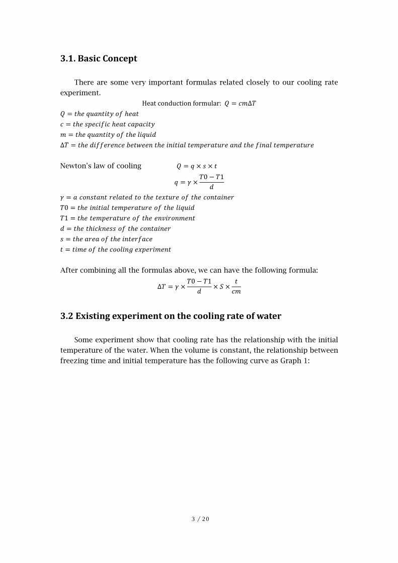
3.2 Existing experiment on the cooling rate of water

Some experiment show that cooling rate has the relationship with the initial

temperature of the water. When the volume is constant, the relationship between

freezing time and initial temperature has the following curve as Graph 1:

4 / 20

After finding some materials about this topic, we find that the cooling rate of

water may have the relationship with the initial temperature, the volumes, the

shape of the container, the material of the container and ambient temperature etc.

3.3.Predictive conclusions

1. If the other factors are treated as constants, the thicker the container is (d↑), the smaller ∆𝑇 will be.

2. If the other factors are treated as constants, then the greater the mass is (m↑), the smaller ∆𝑇 will be.

3. If the other factors are treated as constants, then the larger of the specific

heat capacity, the smaller ∆𝑇 will be.

4. If the other factors are treated as constants, then the higher the initial

temperature is , the larger the ∆𝑇 will be.

4. Methods

4.1. Experiment variables

The key dependent variable of our experiment is the cooling rate of water,

there are many aspects can influent it.

Initial temperature

The tim

e to

freeze (

it

)

Graph 1

5 / 20

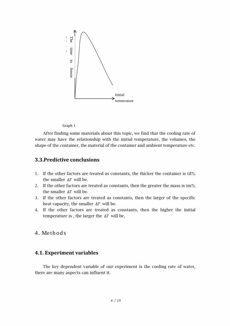
Graph 2 _ fishbone There are mainly three aspects affecting the cooling rate of water: intrinsic

factors of water, environment influences, and anthropic factors. Within each of

these topics, there are still many detail factors; these are reflected in the Graph 2 _

fishbone above.

As our experiments are restricted to many conditions, some of the variables

we can’t control, and other of them are not within our scope of study, so we

explore further the influence of all variables to our experiment and give them

detail analysis.

6 / 20

Table 1

response

variable

(units)

normal

operating level

& range

meas. precision,

accuracy

relationship of

response variable to

objective

Cooling rate 5-10 centigrade

in ten minutes

Thermometer

Precision 0.01

centigrade

Estimate the cooling

condition of

different water

under different

conditions

Table 2

control

variable

(units)

normal level

& range

meas.

precision

& setting error

proposed settings,

based on

predicted effects

predicted

effects

Cooling time

(in minutes) 5-10min

in ten seconds

watch 5 minutes different

Initial

temperature

(1 centigrade)

30-100

centigrade thermometer

Range from

30-100 centigrade

according to

different

experiment

different

solution Water vs.

milk select

Same brand, “Yili”

Milk different

thickness of

the

containers

( in ml)

1-2 layers of

paper cup count

1-2 layers of paper

cup according to

different

experiments

different

Volume of

the liquid 0-200ml

Measuring

cylinder 50-150ml different

Table 3

fixed

factor

(units)

desired

experimental

level &

allowable

range

measurement

precision

How known?

how to

control in experiment

anticipated

effects

Cooling

time

5 minutes

Within 10s

0.1s

stopwatch

Cool water of in

different trails in 5

None to

slight

7 / 20

minutes, time controlled

by stopwatch

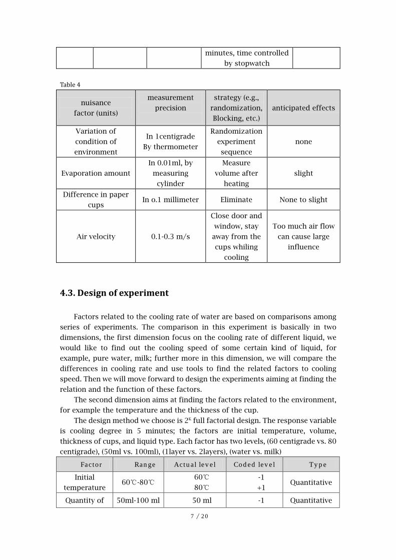
Table 4

nuisance

factor (units)

measurement

precision

strategy (e.g.,

randomization,

Blocking, etc.)

anticipated effects

Variation of

condition of

environment

In 1centigrade

By thermometer

Randomization

experiment

sequence

none

Evaporation amount

In 0.01ml, by

measuring

cylinder

Measure

volume after

heating

slight

Difference in paper

cups In o.1 millimeter Eliminate None to slight

Air velocity 0.1-0.3 m/s

Close door and

window, stay

away from the

cups whiling

cooling

Too much air flow

can cause large

influence

4.3. Design of experiment

Factors related to the cooling rate of water are based on comparisons among

series of experiments. The comparison in this experiment is basically in two

dimensions, the first dimension focus on the cooling rate of different liquid, we

would like to find out the cooling speed of some certain kind of liquid, for

example, pure water, milk; further more in this dimension, we will compare the

differences in cooling rate and use tools to find the related factors to cooling

speed. Then we will move forward to design the experiments aiming at finding the

relation and the function of these factors.

The second dimension aims at finding the factors related to the environment,

for example the temperature and the thickness of the cup.

The design method we choose is 2K full factorial design. The response variable

is cooling degree in 5 minutes; the factors are initial temperature, volume,

thickness of cups, and liquid type. Each factor has two levels, (60 centigrade vs. 80

centigrade), (50ml vs. 100ml), (1layer vs. 2layers), (water vs. milk)

Factor Range Actual level Coded level Type

Initial

temperature 60℃-80℃

60℃

80℃

-1

+1 Quantitative

Quantity of 50ml-100 ml 50 ml -1 Quantitative

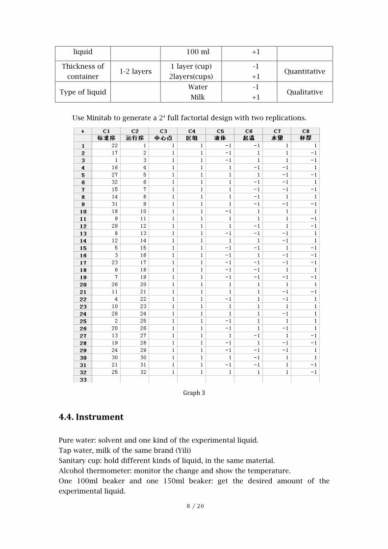
8 / 20

liquid 100 ml +1

Thickness of

container 1-2 layers

1 layer (cup)

2layers(cups)

-1

+1 Quantitative

Type of liquid

Water

Milk

-1

+1 Qualitative

Use Minitab to generate a 24 full factorial design with two replications.

Graph 3

4.4. Instrument

Pure water: solvent and one kind of the experimental liquid.

Tap water, milk of the same brand (Yili)

Sanitary cup: hold different kinds of liquid, in the same material.

Alcohol thermometer: monitor the change and show the temperature.

One 100ml beaker and one 150ml beaker: get the desired amount of the

experimental liquid.

9 / 20

Air thermometer: get the environment temperature and humidity.

4.5. Performing the experiment

In order to improve the efficiency of the experiment, we did some trials to

find proper values for the parameters and ranges.

Considering the availability, samples of 50ml, 60℃ water were used to

choose the time parameter; the experiment was started at the point when the

temperature is 60℃ and after 3min and 5min separately, the ending temperature

was recorded. The difference for 3min was 3℃, and 8℃ for 5 min. Considering

the error of measurement and the significance of the data, 5min was finally

chosen to be the time parameter.

The staring temperature was also adjusted. It was originally desired to set the

to be 70 ℃ and 90 ℃, in the trial experiment, 90℃ was found hard to control,

because the procedure of using the beaker to measure the proper volume and

then pouring into the cups could always lead to a fall below 90℃, and with the

limitation of the instrument, the original temperature of water in the boiler was

not essentially higher than 90℃. With more trials of monitoring the temperature

of water in the boiler and in the cups after the transporting, the range of

temperature was set to be 60℃ and 80℃.

Then, the formal experiment was conducted, first, the temperature of

environment was recorded to be 30.2℃, and the humidity was 23%.

The experiment was carried out according to the randomized sequence. A

beaker was used to take the desired volume of water out from the boiler, then the

water was poured into the numbered cups and the thermometer was used to

monitor the temperature until it fell down to the starting point. Then, start the

timer and wait for 5 minutes, record the ending temperature and do the next one.

As to the milk, it was heated also in the boiler, within its bag. The heated milk

was poured into the beaker to get the desired volume, in order to slow down the

cooling speed in measuring; the beaker was also heated in the water boiler. After

the measurement, the milk was poured into the cup; the thermometer was used to

monitor the temperature until it fell down to the starting point. Then, start the

timer and wait for 5 minutes, record the ending temperature and do the next one.

Perform all the items in the table and record the temperature of the ending

point.

In the whole process, as the experiment was frequently switched between the

water and milk, two beakers were used to measure the volume, and the

instrument used should keep clean. Because the temperature could change very

quickly around the desired points, great attention was paid on monitoring the

temperature.

After the experiment, the temperature of the environment was 31℃. And the

humidity was 24%. This tiny change was not taken into consideration as factors in

the experiment.

10 / 20

5. Analysis

5.1. Data analysis

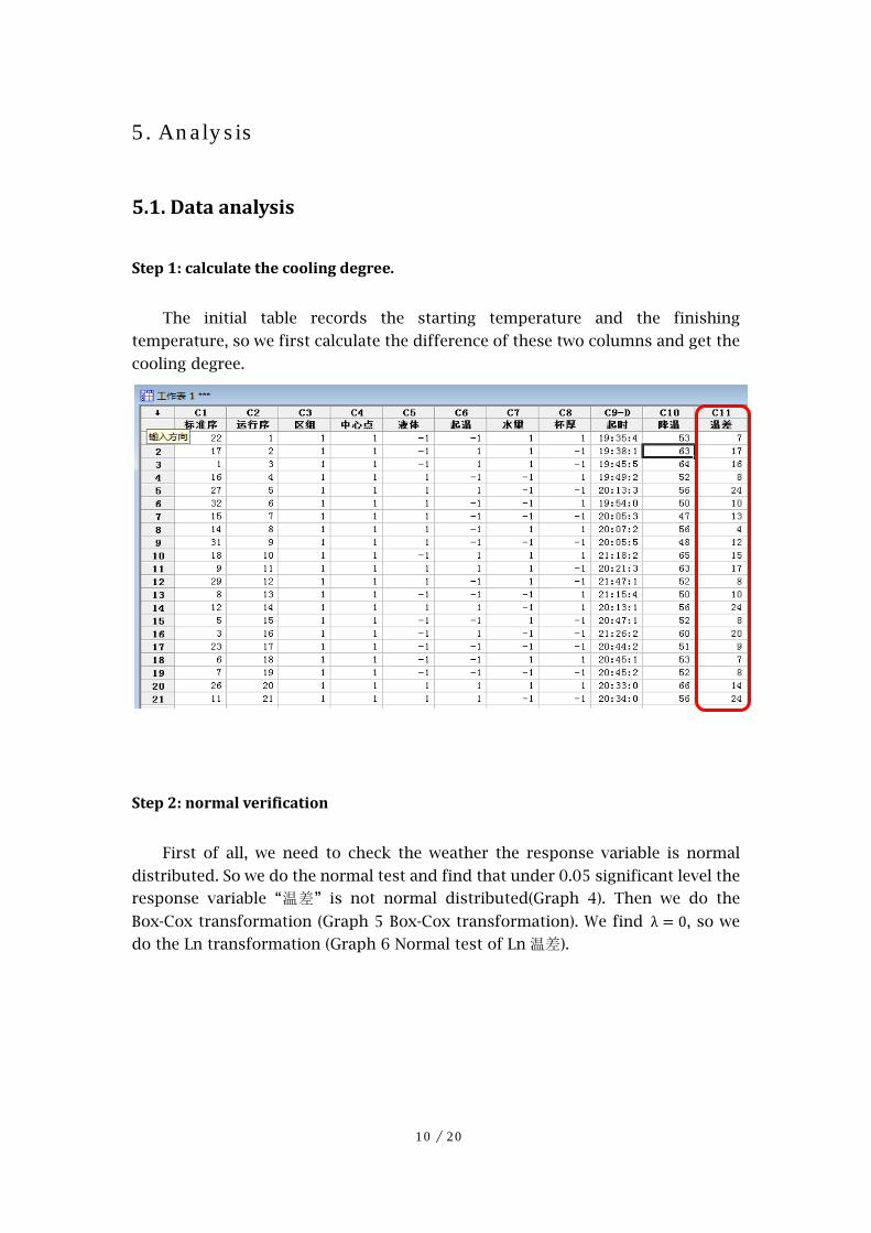
Step 1: calculate the cooling degree.

The initial table records the starting temperature and the finishing

temperature, so we first calculate the difference of these two columns and get the

cooling degree.

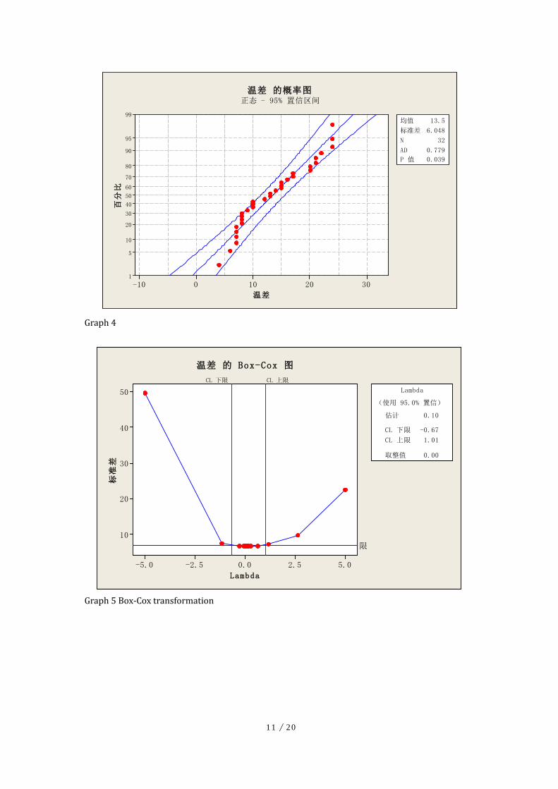
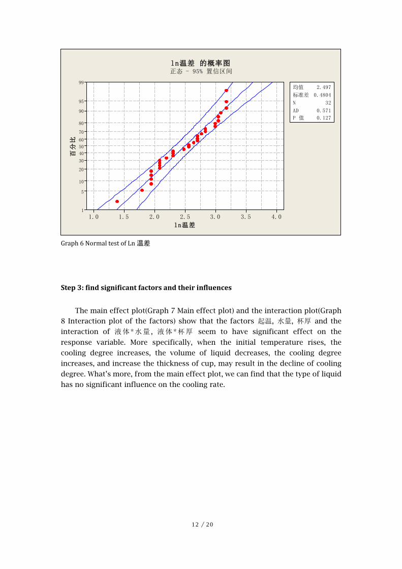
Step 2: normal verification

First of all, we need to check the weather the response variable is normal

distributed. So we do the normal test and find that under 0.05 significant level the

response variable “温差” is not normal distributed(Graph 4). Then we do the

Box-Cox transformation (Graph 5 Box-Cox transformation). We find λ = 0, so we

do the Ln transformation (Graph 6 Normal test of Ln 温差).

11 / 20

Graph 4

Graph 5 Box-Cox transformation

3020100-10

99

95

90

80

70

60

50

40

30

20

10

5

1

温差

百分

比均值 13.5

标准差 6.048

N 32

AD 0.779

P 值 0.039

温差 的概率图正态 - 95% 置信区间

5.02.50.0-2.5-5.0

50

40

30

20

10

Lambda

标准

差

CL 下限 CL 上限

限

估计 0.10

CL 下限 -0.67

CL 上限 1.01

取整值 0.00

（使用 95.0% 置信）

Lambda

温差 的 Box-Cox 图

12 / 20

Graph 6 Normal test of Ln 温差

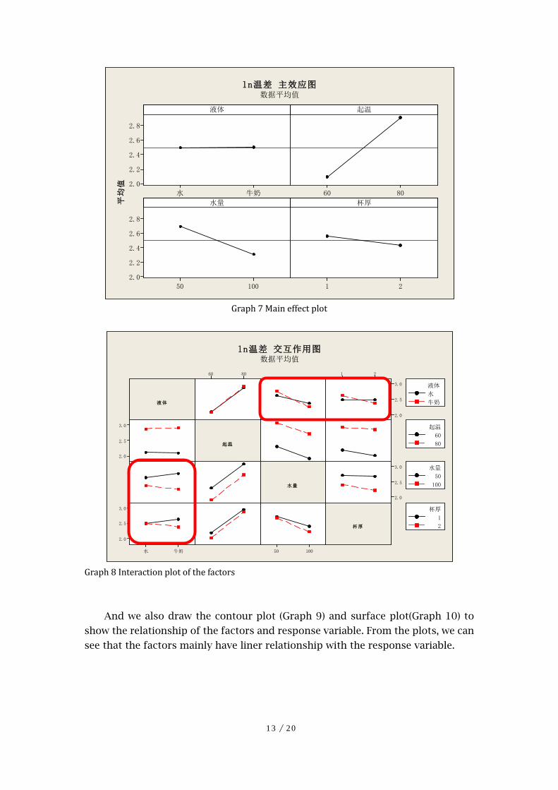
Step 3: find significant factors and their influences

The main effect plot(Graph 7 Main effect plot) and the interaction plot(Graph

8 Interaction plot of the factors) show that the factors 起温, 水量, 杯厚 and the

interaction of 液体*水量 , 液体*杯厚 seem to have significant effect on the

response variable. More specifically, when the initial temperature rises, the

cooling degree increases, the volume of liquid decreases, the cooling degree

increases, and increase the thickness of cup, may result in the decline of cooling

degree. What’s more, from the main effect plot, we can find that the type of liquid

has no significant influence on the cooling rate.

4.03.53.02.52.01.51.0

99

95

90

80

70

60

50

40

30

20

10

5

1

ln温差

百分

比

均值 2.497

标准差 0.4804

N 32

AD 0.571

P 值 0.127

ln温差 的概率图正态 - 95% 置信区间

13 / 20

Graph 7 Main effect plot

Graph 8 Interaction plot of the factors

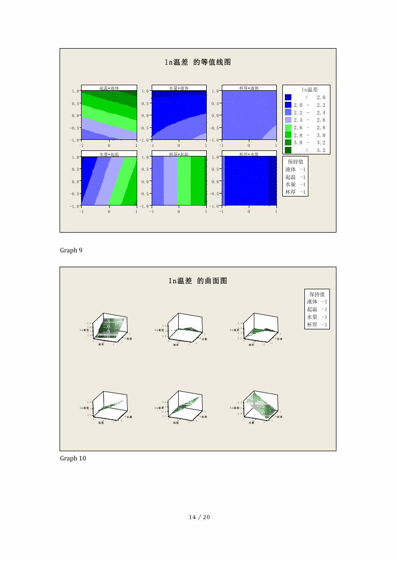
And we also draw the contour plot (Graph 9) and surface plot(Graph 10) to

show the relationship of the factors and response variable. From the plots, we can

see that the factors mainly have liner relationship with the response variable.

牛奶水

2.8

2.6

2.4

2.2

2.08060

10050

2.8

2.6

2.4

2.2

2.021

液体

平均

值

起温

水量 杯厚

ln温差 主效应图数据平均值

8060 21

3.0

2.5

2.0

3.0

2.5

2.0

3.0

2.5

2.0

牛奶水

3.0

2.5

2.0

10050

液体

起温

水量

杯厚

水

牛奶

液体

60

80

起温

50

100

水量

1

2

杯厚

ln温差 交互作用图数据平均值

14 / 20

起温*液体

10-1

1.0

0.5

0.0

-0.5

-1.0

水量*液体

10-1

1.0

0.5

0.0

-0.5

-1.0

杯厚*液体

10-1

1.0

0.5

0.0

-0.5

-1.0

水量*起温

10-1

1.0

0.5

0.0

-0.5

-1.0

杯厚*起温

10-1

1.0

0.5

0.0

-0.5

-1.0

杯厚*水量

10-1

1.0

0.5

0.0

-0.5

-1.0

液体 -1

起温 -1

水量 -1

杯厚 -1

保持值

>

–

–

–

–

–

–

< 2.0

2.0 2.2

2.2 2.4

2.4 2.6

2.6 2.8

2.8 3.0

3.0 3.2

3.2

ln温差

ln温差 的等值线图

Graph 9

12.4

0

2.7

3.0

-1

3.3

0 -11

l n 温差

起温

液体

12.0

0

2.2

2.4

-10 -1

1

l n 温差

水量

液体

1

2.2 0

2.3

2.4

-1

2.5

0 -11

l n 温差

杯厚

液体

1

2.00

2.5

-1

3.0

0 -11

l n 温差

水量

起温

1

2.1 0

2.4

2.7

-1

3.0

0 -11

l n 温差

杯厚

起温

12.0

0

2.1

-1

2.2

0 -11

l n 温差

杯厚

水量

液体 -1

起温 -1

水量 -1

杯厚 -1

保持值

ln温差 的曲面图

Graph 10

15 / 20

Step 4: explore relationship function

The normal probability plot of effect (Figure 8) and the Pareto plot (Figure 9)

have showed the same result that we draw from the main effect plot and

interaction plot.

2520151050-5-10

99

95

90

80

70

60

50

40

30

20

10

5

1

标准化效应

百分

比

A 液体

B 起温

C 水量

D 杯厚

因子 名称

不显著

显著

效应类型

ABD

AD

AC

D

C

B

标准化效应的正态图（响应为 ln温差，Alpha = .05)

Graph 11

A

BCD

ACD

BC

ABCD

AB

ABC

BD

CD

ABD

D

AD

AC

C

B

2520151050

项

标准化效应

2.12

A 液体

B 起温

C 水量

D 杯厚

因子 名称

标准化效应的 Pareto 图（响应为 ln温差，Alpha = .05)

Graph 12

16 / 20

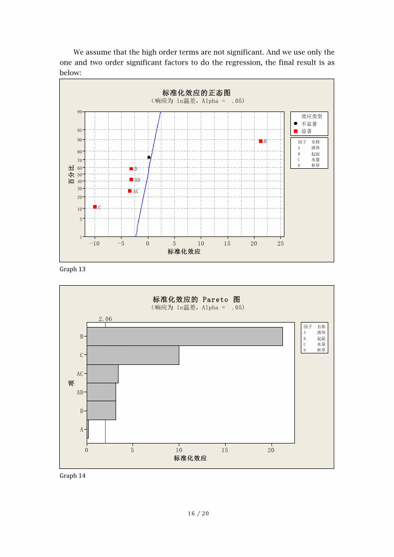
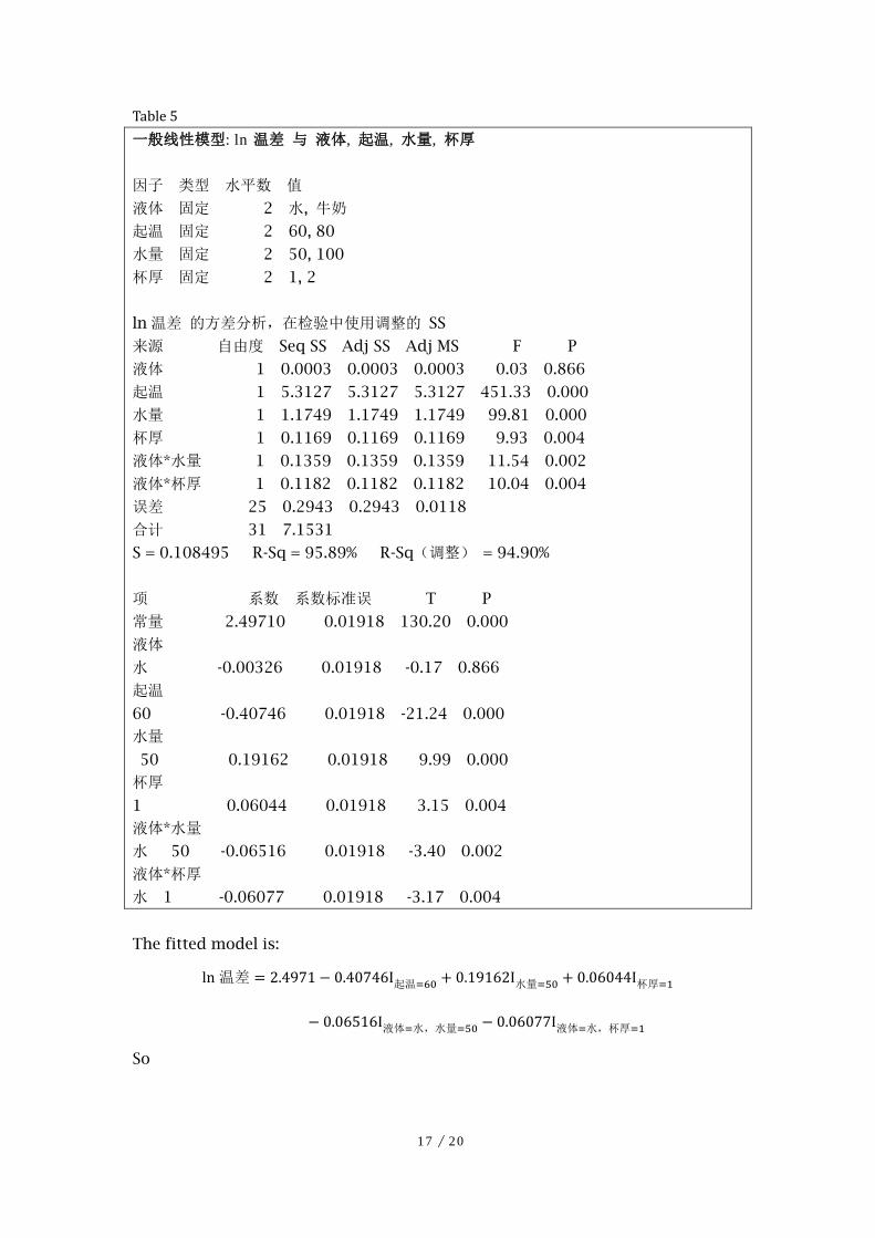
We assume that the high order terms are not significant. And we use only the

one and two order significant factors to do the regression, the final result is as

below:

2520151050-5-10

99

95

90

80

70

60

50

40

30

20

10

5

1

标准化效应

百分

比

A 液体

B 起温

C 水量

D 杯厚

因子 名称

不显著

显著

效应类型

AD

AC

D

C

B

标准化效应的正态图（响应为 ln温差，Alpha = .05)

Graph 13

A

D

AD

AC

C

B

20151050

项

标准化效应

2.06

A 液体

B 起温

C 水量

D 杯厚

因子 名称

标准化效应的 Pareto 图（响应为 ln温差，Alpha = .05)

Graph 14

17 / 20

Table 5 一般线性模型: ln 温差 与 液体, 起温, 水量, 杯厚 因子 类型 水平数 值

液体 固定 2 水, 牛奶

起温 固定 2 60, 80

水量 固定 2 50, 100

杯厚 固定 2 1, 2

ln 温差 的方差分析，在检验中使用调整的 SS

来源 自由度 Seq SS Adj SS Adj MS F P

液体 1 0.0003 0.0003 0.0003 0.03 0.866

起温 1 5.3127 5.3127 5.3127 451.33 0.000

水量 1 1.1749 1.1749 1.1749 99.81 0.000

杯厚 1 0.1169 0.1169 0.1169 9.93 0.004

液体*水量 1 0.1359 0.1359 0.1359 11.54 0.002

液体*杯厚 1 0.1182 0.1182 0.1182 10.04 0.004

误差 25 0.2943 0.2943 0.0118

合计 31 7.1531

S = 0.108495 R-Sq = 95.89% R-Sq（调整） = 94.90%

项 系数 系数标准误 T P

常量 2.49710 0.01918 130.20 0.000

液体

水 -0.00326 0.01918 -0.17 0.866

起温

60 -0.40746 0.01918 -21.24 0.000

水量

50 0.19162 0.01918 9.99 0.000

杯厚

1 0.06044 0.01918 3.15 0.004

液体*水量

水 50 -0.06516 0.01918 -3.40 0.002

液体*杯厚

水 1 -0.06077 0.01918 -3.17 0.004

The fitted model is:

ln 温差 = 2.4971 − 0.40746I起温=60 + 0.19162I水量=50 + 0.06044I杯厚=1

− 0.06516I液体=水，水量=50 − 0.06077I液体=水，杯厚=1

So

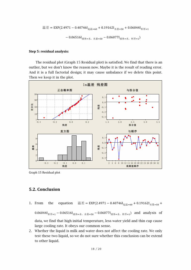
18 / 20

温差 = EXP(2.4971 − 0.40746I起温=60 + 0.19162I水量=50 + 0.06044I杯厚=1

− 0.06516I液体=水，水量=50 − 0.06077I液体=水，杯厚=1)

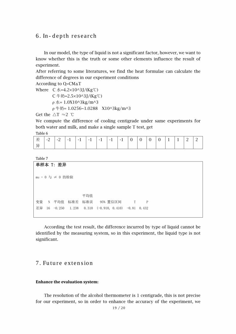
Step 5: residual analysis:

The residual plot (Graph 15 Residual plot) is satisfied. We find that there is an

outlier, but we don’t know the reason now. Maybe it is the result of reading error.

And it is a full factorial design; it may cause unbalance if we delete this point.

Then we keep it in the plot.

Graph 15 Residual plot

5.2. Conclusion

1. From the equation 温差 = EXP(2.4971 − 0.40746I起温=60 + 0.19162I水量=50 +

0.06044I杯厚=1 − 0.06516I液体=水，水量=50 − 0.06077I液体=水，杯厚=1) and analysis of

data, we find that high initial temperature, less water yield and thin cup cause

large cooling rate. It obeys our common sense.

2. Whether the liquid is milk and water does not affect the cooling rate. We only

test these two liquid, so we do not sure whether this conclusion can be extend

to other liquid.

0.20.0-0.2-0.4

99

90

50

10

1

残差

百分

比

3.53.02.52.01.5

0.1

0.0

-0.1

-0.2

-0.3

拟合值

残差

0.10.0-0.1-0.2-0.3

8

6

4

2

0

残差

频率

3230282624222018161412108642

0.1

0.0

-0.1

-0.2

-0.3

观测值顺序

残差

正态概率图 与拟合值

直方图 与顺序

ln温差 残差图

19 / 20

6. In-depth research

In our model, the type of liquid is not a significant factor, however, we want to

know whether this is the truth or some other elements influence the result of

experiment.

After referring to some literatures, we find the heat formulae can calculate the

difference of degrees in our experiment conditions

According to Q=CM△T

Where C 水=4.2×10^3J/(Kg℃)

C 牛奶=2.5×10^3J/(Kg℃)

ρ水= 1.0X10^3kg/m^3

ρ牛奶= 1.0256~1.0288 X10^3kg/m^3

Get the △T ≈2 ℃

We compute the difference of cooling centigrade under same experiments for

both water and milk, and make a single sample T test, get

Table 6 差

异

-2 -2 -1 -1 -1 -1 -1 -1 0 0 0 0 1 1 2 2

Table 7 单样本 T: 差异

mu = 0 与 ≠ 0 的检验

平均值

变量 N 平均值 标准差 标准误 95% 置信区间 T P

差异 16 -0.250 1.238 0.310 (-0.910, 0.410) -0.81 0.432

According the test result, the difference incurred by type of liquid cannot be

identified by the measuring system, so in this experiment, the liquid type is not

significant.

7. Future extension

Enhance the evaluation system:

The resolution of the alcohol thermometer is 1 centigrade, this is not precise

for our experiment, so in order to enhance the accuracy of the experiment, we

20 / 20

need to improve the measuring system.

Extend the experiment parameter range:

Extend the experiment range: choose more types of liquid and extend the range of

initial water, we may get more precise conclusions about cooling rate of different

liquid. Also, under this condition, the factors increase, we need to do fractional

factorial design or Taguchi design to explore the relationships.

8. Reference

http://www.eqna.org/15541/how-does-dissolving-sugar-affect-the-cooling-rate-o

f-water

《水、盐水降温试验及分析计算》刘永胜,杨小林,谢华刚 (河南理工大学土木建筑系,河南焦

作 454003)