SPEECH RECOGNITION FRAMEWORKS

Front End (Eliminate Redundancies) Digital Signal Processing Pre-process the audio signal to enhance speech

and remove noise Extract relevant information for further

processing

Back End (Recognition Algorithms) Phonetic labeling Pattern classification after training Statistical pattern-recognition Grammatical modeling for particular languages Dictionary data bases

DEFINITIONS Semi-stationary: Speech is a slowly

changing (semi-stationary) signal considered to be static in a 20-50 MS time interval

Frame: A 20-50 MS portion of an audio signal

Feature: A calculated attribute of a speech frame

Window: An algorithm to smooth the edges of a frame

Noise: Artifacts in a signal that degrade its clarity

FRONT END (SIGNAL PROCESSING) Resample the simple to match the speech database sample rate

Filter noise Enhance speech characteristics in the signal Separate silence from speech; possibly detect phoneme boundaries

Partition into overlapping frames (about 25 MS with a 50% overlap)

For each frame Apply windowing algorithm to each frame to smooth edges Extract time domain features from the raw signal Extract frequency domain features after applying

transformations to match human perception Possibly apply temporal smoothing algorithms Possibly transform the data to reduce the number of features

Feature normalization (mean to 0, variance to 1)

LML Speech Recognition 2008

4

FourierTransform

FourierTransform

CepstralAnalysis

CepstralAnalysis

PerceptualWeighting

PerceptualWeighting

TimeDerivative

TimeDerivative

Time Derivative

Time Derivative

Energy+

Mel-Spaced Cepstrum

Delta Energy+

Delta Cepstrum

Delta-Delta Energy+

Delta-Delta Cepstrum

Input Speech

• Incorporate knowledge of the nature of speech sounds in measurement of the features.

• Utilize rudimentary models of human perception.

Acoustic Modeling: Feature Extraction Ecample

• Measure features 100 times per sec.

• Use a 25 MS window forfrequency domain analysis.

• Include absolute energy and 12 spectral measurements.

• Time derivatives to model spectral change.

SPEECH FRAMES

Breakup speech signal into overlapping frames

Why? Speech is quasi-

periodic, not periodic, because vocal musculature is always changing

Within a small window of time, we can assume constancy

Typical Characteristics10-30 MS length1/3 – 1/2 overlap

Goal: Extract short-term signal features from speech signal frames

Frame

Frame

Frame

Frame

Frame size

Frame shift

FEATURE EXTRACTION

Definitions Feature: A calculated attribute of a speech signal Phoneme: The smallest phonetic unit that distinguishes

words Morpheme: The smallest phonetic unit that conveys

meaning Feature Extraction: Algorithm to convert a captured

audio into a useable form for decoding Feature Vector: List of values representing a given signal

frame

Process Signal Conditioning (digitizing a signal) Signal Measurement (compute signal amplitudes) Enhance (perform perceptual augmentations) Conversion (Convert data into a feature vector)

Challenge: Choose a relevant and computationally efficient feature set

Goal: Remove redundancies by representing a frame by its feature “fingerprint”

PRINCIPLE COMPONENT ANALYSIS

Normalize the mean of the data set to zero Calculate the covariance matrix and calculate

the eigenvectors (v) and eigenvalues (λ) of that matrixAv = λv (ex:

Sort the eigenvectors (Vi) by eigenvalues Pick the largest eigenvectors and discard those

that remain. Transform the data to a reduced dimension by

performing a dot product (fNewp = )

Feature Dimension Reduction

WHICH AUDIO FEATURES? Cepstrals: They are statistically independent

and phase differences are removed ΔCepstrals, or ΔΔCepstrals: Reflects how

the signal is changing from one frame to the next

Energy: Distinguish the frames that are voiced verses those that are unvoiced

Normalized LPC Coefficients: Represents the shape of the vocal track normalized by vocal tract length for different speakers.

These are some of the popular speech recognition features

9

SIGNAL PROCESSING PROCESSING Acoustic Transducers: Convert sound into an

electronic signal which is then digitized Sampling and Resampling: Down or up sample for

compatibility with stored audio templates Band pass filter: Eliminate frequencies that don’t

contain useful speech information Time Domain Analysis: Extract time domain features Frequency Domain Analysis: Extract frequency

domain features Spectral Normalization: Apply Mel or Bark scale

frequency transformations Cepstral Analysis or Linear Prediction: Each have

a well-defined set of steps Feature Normalization: Normalize the mean,

variance respectively to zero and one. Optionally nomalize the higher statistical moments.

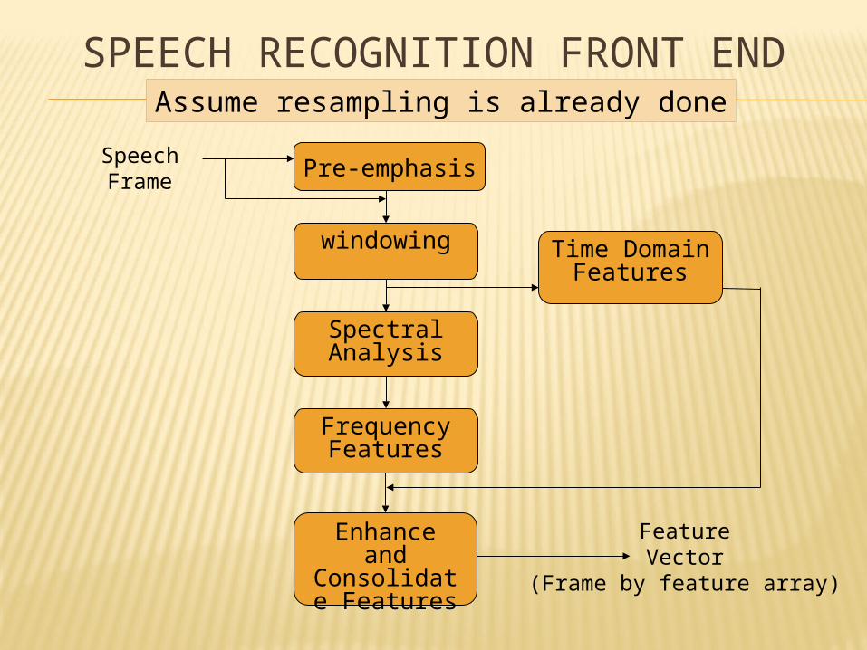
SPEECH RECOGNITION FRONT END

Pre-emphasis

Time DomainFeatures

Enhance and Consolidate

Features

Spectral Analysis

windowing

FrequencyFeatures

SpeechFrame

FeatureVector

(Frame by feature array)

Assume resampling is already done

PRE-EMPHASIS

Human Audio There is an attenuation of the audio signal loudness as it

travels along the cochlea, which makes humans require less amplitudes in the higher frequencies

Speech high frequencies have initial less energy than low frequencies

De-emphasizing the lower frequencies compared to is closer to the way humans hear

Pre-emphasis Algorithm Pre-emphasis recursive filter de-emphasizes lower

frequencies Formula: Y[i] = X[i] - (X[i-1] * δ) 0.95 to 0.97 are common defaults for δ 0.97 de-emphasizes lower frequencies more than 0.95

PRE-EMPHASIS FILTER

y[i] = x[i] – x[i-1] * 0.95

WINDOWING Problem: Framing a signal results in abrupt edges Impact

There is significant spectral leakage in the frequency domain

Large side lobe amplitudes Effect of Windowing

There are no abrupt edges Minimizes side lobe amplitudes and spectral leakage

How? Apply a window formula in the time domain (which is a simple for loop)

Definitions• Frame: A small portion (sub-array) of an audio signal• Window: A frame to which a window function is applied

WINDOW TYPES FOR SPEECH Rectangular: wk = 1 where k = 0 … N

The Naïve approach Advantage: Easy to calculate, array elements unchanged Disadvantage: Messes up the frequency domain

Hamming: wk = 0.54 – 0.46 cos(2kπ/N-1)) Advantage: Fast roll-off in frequency domain, popular for ASR Disadvantage: worse attenuation in stop band

Blackman: wk = 0.42 – 0.5 cos(2kπ/(N-1)) + 0.08 cos(4kπ/(N-1)) Advantage: better attenuation, popular for ASR Disadvantage: wider main lobe

Hanning: wk = 0.5 – 0.5 cos(2kπ/N-1)) Advantage: Useful for pitch transformation algorithms

Multiply the window, point by point, to the audio frame

CREATE AND APPLY HAMMING WINDOW

public double[] createHammingWindow(int filterSize)

{ double[] window = new double[filterSize]; double c = 2*Math.PI / (filterSize - 1); for (int h=0; h<filterSize; h++)

window[h] = 0.54 - 0.46*Math.cos(c*h); return window;

}

public double[] applyWindow(double[] window, double[] signal)

{ for(int i=0; i<window.length; i++) signal[i] = signal[i]*window[i];

return samples; }

RECTANGULAR WINDOW FREQUENCY RESPONSE

Time Domain Filter

BLACKMAN & HAMMING FREQUENCY RESPONSE

TIME DOMAIN FEATURES

Examples Energy Zero-crossing rate Auto correlation and auto

differences Pitch period Fractal Dimension Linear Prediction coefficients

Advantages: less processing; usually easy to understand

Note: These features can directly be obtained from the raw signal

SIGNAL ENERGY

Calculate the short term frame energyEnergy = ∑k=0,N (sk)2 where N is the size of the

frame Represent result in decibels relative to

SPLdb = 10 log(energy)

Tradeoffs If window is too small: too much variance If window is too big: encompasses both

voiced and unvoiced speech

Useful to determine if a windowed frame contains a voiced speech

• Voiced speech has higher energy than unvoiced speech or silence• Changes in energy can indicate stressed syllables (loudness contour)

ZERO CROSSINGS

1. Eliminate a possible DC component, meaning every measurement is offset by some valuea) Average the absolute amplitudes ( 1/M ∑ 0,M-1sk )

b) Subtract the average from each value

2. Count the number of times that the sign changesa) ∑0,M-10.5|sign(sk)-sign(sk-1)|;

where sign(x) = 1 if x≥0, -1 otherwiseb) Note: |sign(sk)-sign(sk-1)| equals 2 if it is a zero

crossing

Unvoiced speech tends to have higher zero crossing than background noise

PITCH DETECTION

• Question: How well does a signal correlate with an offset version of itself?

• Apply the auto-correlation formulaR = ∑i=1,n-z xf[i]xf[i+offset]/∑i=1,F xf[i]2

• Apply the auto-difference formulaD = ∑i=1,n-z Math.abs(xf[i] - xf[i+offset])

• Either method is useful for determining the pitch of a signal. We would expect that R is maximum (and D minimum) when offset corresponds to that of the pitch period

Determine self-similarity of a signal

VOCAL SOURCE Speaker alters vocal tension of the vocal folds

If folds are opened, speech is unvoiced resembling background noise

If folds are stretched close, speech is voiced Air pressure builds and vocal folds blow open releasing

pressure and elasticity causes the vocal folds to fall back Average fundamental frequency (F0): 60 Hz to 300 Hz Speakers control vocal tension alters F0 and the perceived

pitch

Closed Open

Pitch Period

FRACTAL DIMENSION Definition: The self-similarity of a signal Comments

There are various methods to compute a signal’s self-similarity, which each lead to different results

Each method is empirical, not backed by mathematics

Some popular algorithms Box Counting Katz Higuchi

Importance: We would expect that the self-similarity of speech, because it is constrained by the larynx and vocal tract, to be different than that of background noise

BOX COUNTING ALGORITHM

delta = 1FOR i = 0 to S delta = 2^i Cover the curve with rectangles: h = signal[i+delta] – signal[i], w = delta * t Fractal[i] = count of rectangles needed to cover the curvePerform a linear regression on the Fractal arrayThe slope of the best fit line is the fractal dimension

Assume signal[i] is an array of audio amplitudes, where each sample represents t milliseconds

LINEAR REGRESSION

Set of points: (x1,y1), (x2,y2), … (xN,yN)

Equations: Find b0 + b1x1 that minimizes errors where Yi = b0+b1xi+ei

Goal: Find slope b1 of the best fit line

Assumption: the expected value (mean) of the errors is zero

Note: X’ is transpose of X, -1 is inverse

BEST FIT SLOPE OF X AMPLITUDESbestFit(double[] y){ int MAX = y.length;

// Compute the X’X matrix (aij)

double d = MAX*(MAX+1)*(2*MAX+1)/6; // ∑ xi2 = d

double b = MAX * (MAX + 1) / 2; // ∑ xi = b = c

double c = b, a = MAX; // number of points

double sumXY=0, sumY=0; // Compute ∑ yi and sum ∑ xi * yi bi = X’y

for (int i=0; i<MAX; i++) { sumXY += (i+1) * y[i]; sumY += y[i]; }

// Return (X’X)-1 * X’y, where (X’X)-1 is the inverse of X’X

double numerator = -c*sumY + a*sumXY ; // -c*sumXY+a*sumY

double denominator = d * a – b * c; // ad - bc return (denominator == 0) ? 0 : numerator / denominator; // Slope}

Assuming that the x points are 1, 2, 3, …

Note:

Method returns b1 of y = b0 + b1x

KATZ FRACTAL DIMENSION

double katz(double[] x){ int N = x.length;

if (N<=1) return 0;

double L=0, diff=0, D=0;for (int i=1; i<x.length; i++){ L += Math.abs(x[i] - x[i-

1]); diff = Math.abs(x[0] – x[i]);

if (diff > D) D = diff;}double log = Math.log10(N-1);return

(d==0)?0:log/(Math.log10(d/L)+log);}

• L = ∑ xi – xi-1 (sums adjacent lengths)

• max, min = from first point• Katz normalizes log(L)/log(D)) to

use log(L/d)/log(D/d)• Final formula

log(L/d)/log(D/d) = log(N - 1) / log(D/(L/(N-1))) = log(N-1) / (log(D/m) + log(N-1))

• Notes– N-1 because there are N-1

intervals with a signal of N points– L / d = L / (L/(N-1)) = N-1

Dimension = log(sum of lengths)/log(largest distance from the first point)

HIGUCHI FRACTAL DIMENSION

•  

HIGUCHI FRACTAL DIMENSION (CONT)

public double higuchi (double[] x){ int MAX = x.length/4; double[] L = new double[MAX]; for (int k=1; k<=MAX; k++) { L[k-1] = Lk(x, k)/k; } // Find least squares linear best fit of L double slope = bestFit(L, MAX) + 1e-6; return Math.log10(Math.abs(slope));}

double Lk(double[] x, int k){ double sum = 0;

for (int m=1; m<=k; m++){ sum += LmK(x, m, k); }return sum / k;

}double LmK(double[] x, int m, int k){ int N = x.length;

double sum = 0;for (int i=1; i<=(N-m)/k; i++){ sum += Math.abs

(x[m-1+i*k]-x[m-1+(i-1)*k]);

}return sum * (N - 1) / ((N - m)/k

* k);}

LINEAR PREDICTION CODING (LPC)

Originally developed to compress (code) speech Although coding pertains to compression, LPC has

much broader implications LPC is equivalent to the tubal model of the vocal tract

model LPC can be used as a filter to reduce noise (Wiener

filter) from a signal A speech frame can be approximated with a set of LPC

coefficients one coefficient per 1k of sample rate + 2 Example: For a 10k sample, 12 LPC coefficients are

sufficient LPC speech recognition is somewhat noise resilient

ILLUSTRATION: LINEAR PREDICTION

{1, 2, 3, 4, 5, 6, 7, 8, 9, 10, 11, 12, 13, 14, 15, 16}

Goal: Estimate yn using the three previous valuesyn ≈ a1 yn-1 + a2 yn-2 + a3 yn-3

Three ak coefficients, Frame size of 16, 3 coefficientsThirteen equations and three unknowns

Note: No solutions, but LPC finds coeffients with the smallest error

SOLVING N EQUATIONS AND N UNKNOWNS

Gaussian Elimination Complexity: O(n3)

Successive Iteration Complexity varies

Cholesky Decomposition More efficient, still

O(n3) Levenson-Durbin

Complexity: O(n2) Works for symmetric

Toplitz matrices

Definitions for any matrix, ATranspose (AT): Replace aij by aji for all i and jSymmetric: AT = AToplitz: Diagonals to the right all have equal values

COVARIANCE EXAMPLE

Signal: {…, 3, 2, -1, -3, -5, -2, 0, 1, 2, 4, 3, 1, 0, -1, -2, -4, -1, 0, 3, 1, 0, …}

Frame: {-5, -2, 0, 1, 2, 4, 3, 1}, Number of coefficients: 3 φ(1,1) = -3*-3 +-5*-5 + -2*-2 + 0*0 + 1*1 + 2*2 + 4*4 + 3*3 = 68 φ(2,1) = -1*-3 +-3*-5 + -5*-2 + -2*0 + 0*1 + 1*2 + 2*4 + 4*3 = 50 φ(3,1) = 2*-3 +-1*-5 + -3*-2 + -5*0 + -2*1 + 0*2 + 1*4 + 2*3 = 13 φ(1,2) = -3*-1 +-5*-3 + -2*-5 + 0*-2 + 1*0 + 2*1 + 4*2 + 3*4 = 50 φ(2,2) = -1*-1 +-3*-3 + -5*-5 + -2*-2 + 0*0 + 1*1 + 2*2 + 4*4 = 60 φ(3,2) = 2*-1 +-1*-3 + -3*-5 + -5*-2 + -2*0 + 0*1 + 1*2 + 2*4 = 36 φ(1,3) = -3*2 +-5*-1 + -2*-3 + 0*-5 + 1*-2 + 2*0 + 4*1 + 3*2 = 13 φ(2,3) = -1*2 +-3*-1 + -5*-3 + -2*-5 + 0*-2 + 1*0 + 2*1 + 4*2 = 36 φ(3,3) = 2*2 +-1*-1 + -3*-3 + -5*-5 + -2*-2 + 0*0 + 1*1 + 2*2 = 48 φ(1,0) = -3*-5 +-5*-2 + -2*0 + 0*1 + 1*2 + 2*4 + 4*3 + 3*1 = 50 φ(2,0) = -1*-5 +-3*-2 + -5*0 + -2*1 + 0*2 + 1*4 + 2*3 + 4*1 = 23 φ(3,0) = 2*-5 +-1*-2 + -3*0 + -5*1 + -2*2 + 0*4 + 1*3 + 2*1 = -12

Note: φ(j,k) = ∑n=start,start+N-1 yn-kyn-j

AUTO CORRELATION EXAMPLE

Signal: {…, 3, 2, -1, -3, -5, -2, 0, 1, 2, 4, 3, 1, 0, -1, -2, -4, -1, 0, 3, 1, 0, …}

Frame: {-5, -2, 0, 1, 2, 4, 3, 1}, Number of coefficients: 3

R(0) = -5*-5 + -2*-2 + 0*0 + 1*1 + 2*2 + 4*4 + 3*3 + 1*1 = 60 R(1) = -5*-2 + -2*0 + 0*1 + 1*2 + 2*4 + 4*3 + 3*1 = 35 R(2) = -5*0 + -2*1 + 0*2 + 1*4 + 2*3 + 4*1 = 12 R(3) = -5*1 + -2*2 + 0*4 + 1*3 + 2*1 = -4

Note: φ(j,k)=∑n=0,N-1-(j-k) ynyn+(j-k)=R(j-k)

Assumption: all entries before and after the frame treated as zero

LPC FEATURES AS A FRONT END

Assumptions Future discrete signal samples are functions of the

previous ones The speech signal is purely linear (interactions with other

signials add or subtract, but don’t multiply)

Coefficients: Generally eight to fourteen LPC coefficients are sufficient to represent a particular block of sound samples

Disadvantage: Linear prediction coefficients tend to be less stable other methods (ex: Cepstral analysis).

Enhancement: Perceptual Linear Prediction uses both frequency and time domain data. The result is comparable to Cepstral analysis. Rasta Linear Prediction also filters adjacent samples for an additional enhancement.

THE LPC SPECTRUM

1. Perform a LPC analysis2. Find the poles3. Plot the spectrum around

the z-Plane unit circle

What do we find concerning the LPC spectrum?1. Adding poles better matches speech up to about 18 for a 16k sampling rate2. The peaks tend to be overly sharp (“spiky”) because small radius changes

greatly alters pole skirt widths in the z-plane

FILTER BANK FRONT END The bank consists of twenty to thirty overlapping

band pass filters spread along the warped frequency axis

Represent spectrum with log-energy output from filter bank

Each frequency bank F handles frequencies from f-i to f+i or individual ranges of frequencies that models the rows of hair bands in the cochlea

The feature data is an array of energy values obtained from each filter

Result: Good idea, but it has not proven to be as effective as other methods

WARPED BAND PASS FILTER SET

Mel frequency warping

Original Spectrum

SIGNAL FILTERS

PURPOSES (GENERAL) EXAMPLES Separate Signals Eliminate distortions Remove unwanted data Compress and decompress Extract important features Enhance desired components

Eliminate frequencies without speech information

Enhance poor quality recordings

Reduce background Noise Adjust frequencies to mimic

human perception

How? Execute a convolution algorithm

CONVOLUTIONpublic static double[] convolution(double[] x, double[] b, double[] a){ double[] y = new double[x.length + b.length - 1];

for (int i = 0; i < x.length; i ++) { for (int j = 0; j < b.length; j++) { if (i-j>=0) y[i] += b[j] * x[i - j]; } if (a!=null) { for (int j = 1; j < a.length; j ++) { if (i-j>=0) y[i] -= a[j] * y[i - j]; } } } return y;}

The algorithm for creating Time Domain filters

Notes: The symbol x commonly represents the raw time domain signalThe symbol Y represents the filterd signalCapital X represents the frequency domain spectrum

TIME DOMAIN FILTERS Finite Impulse Response

Filter only affects the data samples, hence the filter only effects a fixed number of data point

y[n] = b0 sn+ b1 sn-1+ …+ bM-1 sn-M+1=∑k=0,M-1bk sn-k

Infinite Impulse Response (also called recursive) Filter affects the data samples and previous filtered

output, hence the effect can be infinite t[n] = ∑k=0,M-1bk sn-k + ∑k=0,M-1 ak tn-k

If a signal was linear, so is the filtered signal Why? We summed samples multiplied by constants,

we didn’t multiply or raise samples to a power

CONVOLUTION THEOREM

Multiplication in the time domain is equivalent to convolution in the frequency domain

Multiplication in the frequency domain equivalent to convolution in the time domain

Application: We can design a filter by creating its desired frequency response and then perform an inverse FFT to derive the filter kernel

Theoretically, we can create an ideal (“perfect”) low pass filter with this approach

AMPLIFY

Top Figure (original signal)

Bottom Figure The signal’s amplitude

is multiplied by 1.6 Attenuation can occur

by picking a magnitude that is less than one

y[n] = k δ[n]

MOVING AVERAGE FIR FILTER

int[] average(int x[]) { int[] y[x.length]; for (int i=50; i<x.length-50; i++) { for (int j=-50; j<=50; j++) { y[i] += x[i + j]; } y[i] /= 101;} }

Convolution using a simple filter kernel

Formula:

Example Point:

Example Point (Centered):

IIR (RECURSIVE) MOVING AVERAGE

Example:y[50] = (x[47]+x[48]+x[49]+x[50]+x[51]+x[52]+x[53])/7y[51] = (x[48]+x[49]+x[50]+x[51]+x[52]+x[53]+x[54])/7 = y[50] + (x[54] – x[47])/7

The general casey[i] = y[i-1] + (x[i+M/2] - x[i-(M+1)/2])/M

Two additions per point no matter the length of the filter

Note: Integers work best with this approach to avoid round off drift

MOVING AVERAGE FILTER CHARACTERISTICS

Longer kernel filters more noise Long filters lose edge sharpness Distorts the frequency domain Very fast Frequency response

sync function (sin(x)/x) A degrading sine wave

Speech Great for smoothing a pitch

contour Horrible for identifying formants

TIME DOMAIN FILTERING Band Pass

Filter frequencies below the minimum fundamental frequency (F0)

Filter frequencies above the speech range (≈4kHz)

Linear smoother and median of five filters Used in combination to smooth the pitch contour

Derivative (slope) filter Measure changes in a given feature from one

frame to another Tends to reduce the effects of noise in ASR

Noise Removal: Separate set of slides

BAND PASS FILTERS

Butterworth Advantages:

IIR filter, which is fast minimal ripple

Disadvantage: slow transition Window Sync

Advantage: quick transition Disadvantages

FIR filter, which is slow Ripples in the pass band

Many other filters with various advantages and disadvantages. Open source code for these exist.

ACORNS uses both Butterworth and Window Sync filters

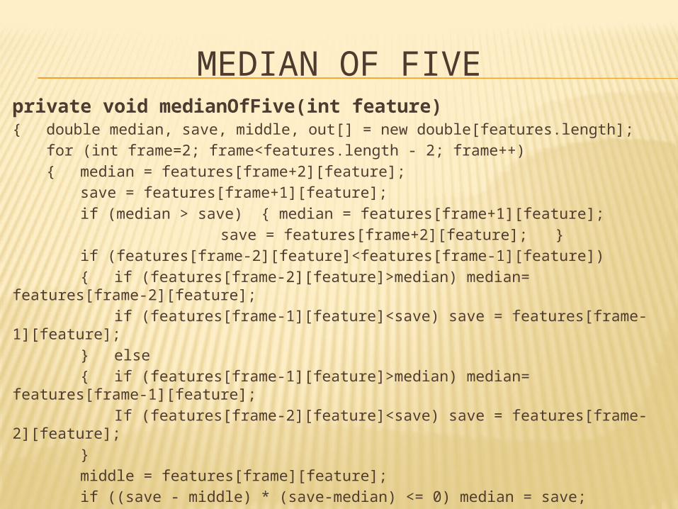
MEDIAN OF FIVEprivate void medianOfFive(int feature){ double median, save, middle, out[] = new double[features.length];

for (int frame=2; frame<features.length - 2; frame++){ median = features[frame+2][feature];

save = features[frame+1][feature];if (median > save) { median = features[frame+1][feature];

save = features[frame+2][feature]; }if (features[frame-2][feature]<features[frame-1][feature]){ if (features[frame-2][feature]>median) median=

features[frame-2][feature];if (features[frame-1][feature]<save) save =

features[frame-1][feature];} else{ if (features[frame-1][feature]>median) median=

features[frame-1][feature];If (features[frame-2][feature]<save) save =

features[frame-2][feature];}middle = features[frame][feature];if ((save - middle) * (save-median) <= 0) median = save;if ((middle - save) * (middle - median) <= 0) median = middle;out[frame] = median;

}

LINEAR SMOOTHER

private double[] linearSmoother(int frame, double[][] frames, int

feature){

double[] out = new double[features.length];for (int feature = 2;

frame<frames[frame].length; frame++){

out[feature] = frames[frame][feature]/4+ frames[frame-1][feature]/2 + frames[frame-2][feature]/4;

}return out;

}

DERIVATIVE FILTER

private void calculateDynamicFeatures(int featureOffset){ int start, end;

double numerator, denominator;for (int frame=0; frame<features.length; frame++){ numerator = denominator = 0; start = (frame<D) ? -frame: - D; end = (frame>=features.length - D) ? features.length - frame - 1:

+D; for (int d= start; d<= end; d++) { numerator += d * features[frame + d][feature];

denominator += d * d; } if (denominator !=0) out[frame][feature] = numerator /

denominator;} }

Computes slope over 2D+1 frames

FILTER CHARACTERISTICS

Note: The ideal filter would require infinite computation

FILTER TERMINOLOGY

Rise time: Time for step response to go from 10% to 90% Linear phase: Rising edges match falling edges Overshoot: amount amplitude exceeds the desired value Ripple: pass band oscillations Ringing: stop band oscillations Pass band: the allowed frequencies Stop band: the blocked frequencies Transition band: frequencies between pass or stop bands Cutoff frequency: point between pass and transition

bands Roll off: transition sharpness between pass and stop bands Stop band attenuation: reduced amplitude in the stop

band

FILTER PERFORMANCE