journals.sagepub.com/home/jae free jet generating two ...

Article

Numerical study of the flowand the near acoustic fieldsof an underexpanded roundfree jet generating twoscreech tones

Romain Gojon and Christophe Bogey

Abstract

The flow and near acoustic fields of a supersonic round free jet are explored using a compressible

large eddy simulation. At the exit of a straight pipe nozzle, the jet is underexpanded, and is

characterized by a Nozzle Pressure Ratio of 4.03 and a Temperature Ratio of 1. It has a fully

expanded Mach number of 1.56, an exit Mach number of 1, and a Reynolds number of 6�104.

Flow snapshots, mean flow fields and convection velocity in the jet shear layers are consistent

with experimental data and theoretical results. Furthermore, two screech tones are found to

emerge in the pressure spectrum calculated close to the nozzle. Using a Fourier decomposition of

the pressure fields, the two screech tones are found to be associated with anticlockwise helical

oscillation modes. Besides, the frequencies of the screech tones and the associated oscillation

modes both agree with theoretical predictions and measurements. Moreover, pressure fields

filtered at the screech frequencies reveal the presence of hydrodynamic-acoustic standing

waves. In those waves, the regions of highest amplitude in the jet are located in the fifth and

the sixth cells of the shock cell structure. The two screech tones therefore seem to be linked to

two different loops established between the nozzle and the fifth and sixth shock cells, respectively.

In the pressure fields, three other acoustic components, namely the low-frequency mixing noise,

the high-frequency mixing noise and the broadband shock-associated noise, are noted. The

directivity and frequency of the mixing noise are in line with numerical and experimental studies.

A production mechanism of the mixing noise consisting of sudden intrusions of turbulent struc-

tures into the potential core is discussed. Then, the broadband shock-associated noise is studied.

This noise component is due to the interactions between the turbulent structure in the shear

layers and the shocks in the jet. By analyzing the near pressure fields, this noise component is

found to be produced mainly in the sixth shock cell. Finally, using the size of this shock cell in the

Laboratoire de Mecanique des Fluides et d’Acoustique, UMR CNRS 5509, Ecole Centrale de Lyon, Universite de Lyon,

Ecully Cedex, France

Corresponding author:

Romain Gojon, Laboratoire de Mecanique des Fluides et d’Acoustique, UMR CNRS 5509, Ecole Centrale de Lyon,

Universite de Lyon, 69134 Ecully Cedex, France.

Email: [email protected]

International Journal of Aeroacoustics

2017, Vol. 16(7–8) 603–625

! The Author(s) 2017

Reprints and permissions:

sagepub.co.uk/journalsPermissions.nav

DOI: 10.1177/1475472X17727606

journals.sagepub.com/home/jae

https://uk.sagepub.com/en-gb/journals-permissions

https://doi.org/10.1177/1475472X17727606

journals.sagepub.com/home/jae

classical theoretical model of this noise component, a good agreement is found with the simu-

lation results.

Keywords

Large eddy simulation, supersonic jet, screech

Date received: 9 September 2016; accepted: 1 June 2017

Introduction

In non-ideally expanded supersonic jets, several acoustic components including screechnoise, mixing noise and broadband shock-associated noise are observed. The screech noiseis due to an aeroacoustic feedback mechanism established between the turbulent structurespropagating downstream and the acoustic waves propagating upstream. This mechanismwas described by Powell,1 then by Raman,2 who proposed that the turbulent structuresdeveloping in the jet shear layers and propagating in the downstream direction interactwith the quasi-periodic shock cell structure of the jet, creating upstream propagating acous-tic waves. The resonant loop is closed at the nozzle lips where sound waves are reflected backand excite the shear layers. Moreover, for round jets, Powell1 identified four modes, labeledA, B, C, and D, on the basis of the screech frequency evolution with the ideally expandedMach number Mj. Each mode is dominant for a specific ideally expanded Mach numberrange and frequency jumps are noted between the modes. Later, Merle3 showed that mode Acan be divided into modes A1 and A2. Davies and Oldfield4 studied the oscillation modes ofthe jets associated with the five screech modes. They found that A1 and A2 modes are linkedto axisymmetric oscillation modes of the jet, B to sinuous and sometimes helical modes, C tohelical modes and D to sinuous modes. Mixing noise is observed in both subsonic5 andsupersonic6 jets. The dominant Strouhal number of this noise component is around 0.2 andits directivity is well marked around angles of 20� with respect to the downstream direction.This component is mainly generated at the end of the potential core.7,8,9 For subsonic jets,Bogey et al.10 and Bogey and Bailly7 proposed that this acoustic component is due to theintermittent intrusion of turbulent structures into the potential core. The broadband shock-associated noise is produced by the interactions between the turbulence and the shock cellstructure. Martlew11 was the first to clearly identify this noise. Its central frequency varieswith the angle in the far field, according to experiments.12–14 Harper-Bourne and Fisher15

proposed a model which permits to predict the central frequency of this noise component asa function of the observation angle.

In the present work, the LES of a round supersonic underexpanded jet is carried out inorder to investigate the acoustic mechanisms in non-ideally expanded jets. The jet corres-ponds to the reference free jet in a study on impinging jets performed by Gojon et al.16 Theresults from this jet were also used to generate schlieren-like images, in a study of Castelainet al.,17 in order to asses the quality of the estimation of the convection velocity in the jetshear layers using schlieren pictures in experiments. In the present paper, the spectral andhydrodynamic properties of the jet are described and compared with experimental data andmodels. Three acoustic components, namely the screech noise, the mixing noise, and thebroadband shock-associated noise, are investigated. In particular, two screech tones arefound in the spectra calculated in the vicinity of the nozzle. The causes of such a result

604 International Journal of Aeroacoustics 16(7–8)

are sought. The production mechanism of the mixing noise is then investigated by evaluatingskewness and kurtosis factors of the fluctuating pressure. Finally, the broadband shock-associated noise is examined. Notably, a discussion about the lengthscale to use in theclassical model of this noise component is conducted. The paper is organized as follows.The jet parameters and the numerical methods used for the LES are given in the Parameterssection. The aerodynamic results are analyzed in the Aerodynamic results section, and theacoustic mechanisms are investigated in the Acoustic results section. Concluding remarks areprovided in the last section.

Parameters

Jets parameters

The large-eddy simulation of a round supersonic jet is performed. The jet originates from astraight pipe nozzle of radius r0, whose lip is 0:1r0 thick. The jet is underexpanded, and hasa Nozzle Pressure Ratio of NPR ¼ Pr=Pamb ¼ 4:03 and a Temperature RatioTR ¼ Tr=Tamb ¼ 1, where Pr and Tr are the stagnation pressure and temperature andPamb and Tamb are the ambient values. As for a jet generated by a convergent nozzle,the exit Mach number of the present jet isMe ¼ ue=ce ¼ 1, where ue and ce are the velocityand speed of sound in the jet. Moreover, the jet is characterized by a fully expanded Machnumber of Mj ¼ uj=cj ¼ 1:56, where uj and cj are the velocity and the speed of sound inthe ideally expanded equivalent jet. Its Reynolds number is Rej ¼ ujDj=� ¼ 6� 104, whereDj is the nozzle diameter of the ideally expanded equivalent jet and � is the kinematicmolecular viscosity. At the nozzle inlet, a Blasius boundary-layer profile with a thicknessof 0:15r0 and a Crocco-Busemann profile are imposed for velocity and density. The exitconditions of the jet and the nozzle lip thickness are similar to those in the experiments ofHenderson et al.18 Finally, low-amplitude vortical disturbances, not correlated in the azi-muthal direction,19 are added in the boundary layer in the nozzle, at z ¼ �0:5r0, in orderto generate velocity fluctuations at the nozzle exit. The strength of the forcing is chosen inorder to obtain turbulent intensities of around 6% of the fully expanded jet velocity at thenozzle exit.

Numerical parameters

The LES is performed by solving the unsteady compressible Navier–Stokes equations on acylindrical mesh ðr, �, zÞ. An explicit six-stage Runge–Kutta algorithm and low-dispersionand low-dissipation explicit eleven-point finite differences are used for time integration andspatial derivation,20,21 respectively. At the end of each time step, a high-order filtering isapplied to the flow variables in order to remove grid-to-grid oscillations and to dissipatesubgrid-scale turbulent energy. The filtering thus acts as a subgrid scale model.22–25 Theradiation conditions of Tam and Dong26 are implemented at the boundaries of the com-putational domain. A sponge zone combining grid stretching and Laplacian filtering is alsoemployed to damp the turbulent fluctuations before they reach the boundaries. Moreover,non-slip adiabatic conditions are used to simulate the nozzle walls. In order to increase thetime step of the simulation, the effective resolution near the origin of the cylindricalcoordinates is reduced.27 The axis singularity is treated with the method of Mohseniand Colonius.28 Finally, a shock-capturing filtering is used in order to avoid Gibbs oscil-lations near shocks. It consists in applying a conservative second-order filter at a

Gojon and Bogey 605

magnitude determined each time step using a shock sensor.29 It was successfully used byCacqueray et al.30 for the LES of an overexpanded jet at an equivalent Mach number ofMj ¼ 3:3.

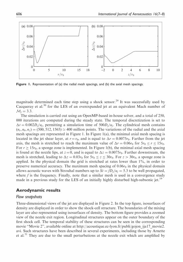
The simulation is carried out using an OpenMP-based in-house solver, and a total of 250,000 iterations are computed during the steady state. The temporal discretization is set to�t ¼ 0:002Dj=uj, permitting a simulation time of 500Dj=uj. The cylindrical mesh containsðnr, n�, nzÞ ¼ ð500, 512, 1565Þ ’ 400 million points. The variations of the radial and the axialmesh spacings are represented in Figure 1. In Figure 1(a), the minimal axial mesh spacing islocated in the jet shear layer, at r¼ r0, and is equal to �r ¼ 0:0075r0. Farther from the jetaxis, the mesh is stretched to reach the maximum value of �r ¼ 0:06r0 for 5r0 � r � 15r0.For r � 15r0, a sponge zone is implemented. In Figure 1(b), the minimal axial mesh spacingis found at the nozzle lips, at z¼ 0, and is equal to �z ¼ 0:0075r0. Farther downstream, themesh is stretched, leading to �z ¼ 0:03r0 for 5r0 � z � 30r0. For z4 30r0, a sponge zone isapplied. In the physical domain the grid is stretched at rates lower than 1%, in order topreserve numerical accuracy. The maximum mesh spacing of 0:06r0 in the physical domainallows acoustic waves with Strouhal numbers up to St ¼ fDj=uj ¼ 5:3 to be well propagated,where f is the frequency. Finally, note that a similar mesh is used in a convergence studymade in a previous study for the LES of an initially highly disturbed high-subsonic jet.19

Aerodynamic results

Flow snapshots

Three-dimensional views of the jet are displayed in Figure 2. In the top figure, isosurfaces ofdensity are displayed in order to show the shock-cell structure. The boundaries of the mixinglayer are also represented using isosurfaces of density. The bottom figure provides a zoomedview of the nozzle exit region. Longitudinal structures appear on the outer boundary of thefirst shock cell. The temporal stability of these structures can be seen in the correspondingmovie ‘‘Movie 2’’, available online at http://acoustique.ec-lyon.fr/publi/gojon_ija17_movie2.avi. Such structures have been described in several experiments, including those by Arnetteet al.31 They are due to the small perturbations at the nozzle exit which are amplified by

0 5 10 15 180

0.02

0.04

0.06

0.08(a)

r/r0

Δr/

r 0

−2 0 2 4 6 8 100

0.02

0.04

0.06

0.08(b)

z/r0

Δz/

r 0

Figure 1. Representation of (a) the radial mesh spacings, and (b) the axial mesh spacings.


http://acoustique.ec-lyon.fr/publi/gojon_ija17_movie2.avi


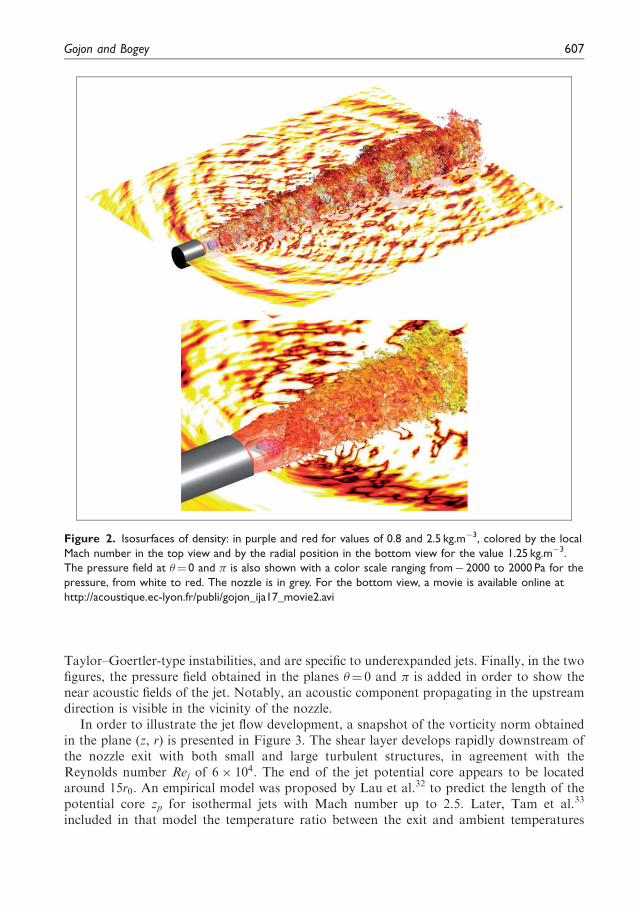
Taylor–Goertler-type instabilities, and are specific to underexpanded jets. Finally, in the twofigures, the pressure field obtained in the planes �¼ 0 and � is added in order to show thenear acoustic fields of the jet. Notably, an acoustic component propagating in the upstreamdirection is visible in the vicinity of the nozzle.

In order to illustrate the jet flow development, a snapshot of the vorticity norm obtainedin the plane (z, r) is presented in Figure 3. The shear layer develops rapidly downstream ofthe nozzle exit with both small and large turbulent structures, in agreement with theReynolds number Rej of 6� 104. The end of the jet potential core appears to be locatedaround 15r0. An empirical model was proposed by Lau et al.32 to predict the length of thepotential core zp for isothermal jets with Mach number up to 2.5. Later, Tam et al.33

included in that model the temperature ratio between the exit and ambient temperatures

Figure 2. Isosurfaces of density: in purple and red for values of 0.8 and 2.5 kg.m�3, colored by the local

Mach number in the top view and by the radial position in the bottom view for the value 1.25 kg.m�3.

The pressure field at �¼ 0 and � is also shown with a color scale ranging from� 2000 to 2000 Pa for the

pressure, from white to red. The nozzle is in grey. For the bottom view, a movie is available online at


Gojon and Bogey 607

in order to take into account compressibility effects. For the present jet, where the exittemperature Te is lower than the ambient temperature Tamb, the model can be written

zpDj¼ 4:2þ 1:1M2

j þ 1:1 1�Te

Tamb

� �ð1Þ

For the present jet, equation (1) yields zp ¼ 15:6r0, which is in good agreement with theresult of the simulation.

A snapshot of the density and fluctuating pressure obtained in the (z, r) plane is providedin Figure 4(a). A movie, labeled ‘‘Movie 1’’, showing the temporal evolution of the jet is alsoavailable online at http://acoustique.ec-lyon.fr/publi/gojon_ija17_movie1.avi. A shock-cellstructure, typical of an underexpanded jet, is observed in the density field. It contains around10 shock cells. Because the jet is strongly underexpanded with a NPR of 4.03, a Mach disk isfound in the first cell, at z ¼ 2:35r0. This is in agreement with the results of Powell,34

Henderson,35 and Addy,36 who noted that a Mach disk is generated in underexpandedjets for NPR> 3.8 or 3.9. For the comparison, a Schlieren picture of an underexpandedjet obtained by Andre et al.37 is displayed in Figure 4(b). The fully expanded Mach numberof the jet is Mj ¼ 1:55 and the exit Mach number is Me ¼ 1. A strong similarity appearswith notably the presence of a Mach disk in the first cell. In the pressure field, in Figure 4(a),two acoustic contributions appear. First, circular wavefronts seem to originate from the firstfive cells. They are due to the interactions between the shocks and the turbulence in the shearlayers. Upstream propagating acoustic waves are also observed in the vicinity of the nozzle.

Mean fields

The mean axial and radial velocity fields of the jet are presented in Figure 5, where theexperimental PIV results of Andre et al.37 are also displayed for aMj ¼ 1:5 andMe ¼ 1 jet.The shock-cell structure and the levels obtained in the LES and in the experiment are in goodagreement. The mean total velocity field in the (z, r) plane is shown in Figure 6. It comparesvery well with the experimental results of Henderson et al.18 for a jet with similar exitconditions.

In Figures 5 and 6, the length Ls of the first shock cell of the jet is approximately 3:20r0.This result is identical to those obtained by Andre et al.37 and of Henderson et al.18 for

Figure 3. Snapshot of the vorticity norm j!j obtained in the (z, r) plane. The colour scale ranges up to

the level of 10uj=Dj, from white to red. The nozzle is in black.



similar jets. Moreover, this length can be estimated by using a first-order shock solutionbased on the pressure ratio ps=pa, where ps is the pressure perturbation of the shock-cellstructure and ps þ pa is the pressure in the jet. This model was proposed by Prandtl38 in 1904.Later, the following approximated solution was given by Pack39

Ls ’ 1:22�Dj ð2Þ

where � ¼ffiffiffiffiffiffiffiffiffiffiffiffiffiffiffiffiM

2j � 1

q. For the present jet, equation (2) provides Ls ¼ 3:20r0, which is iden-

tical to the value reported above.

Figure 4. (a) Snapshot of the density in the jet and of the fluctuating pressure. The colour scale ranges

from 1 to 3 kg.m�3 for the density, from blue to red, and from –2000 to 2000 Pa for the pressure, from

white to black; (b) Schlieren picture of an underexpanded jet obtained by Andre et al.37 for aMj ¼ 1:55

andMe ¼ 1 jet; a movie is available online at http://acoustique.ec-lyon.fr/publi/gojon_ija17_movie1.avi

Gojon and Bogey 609

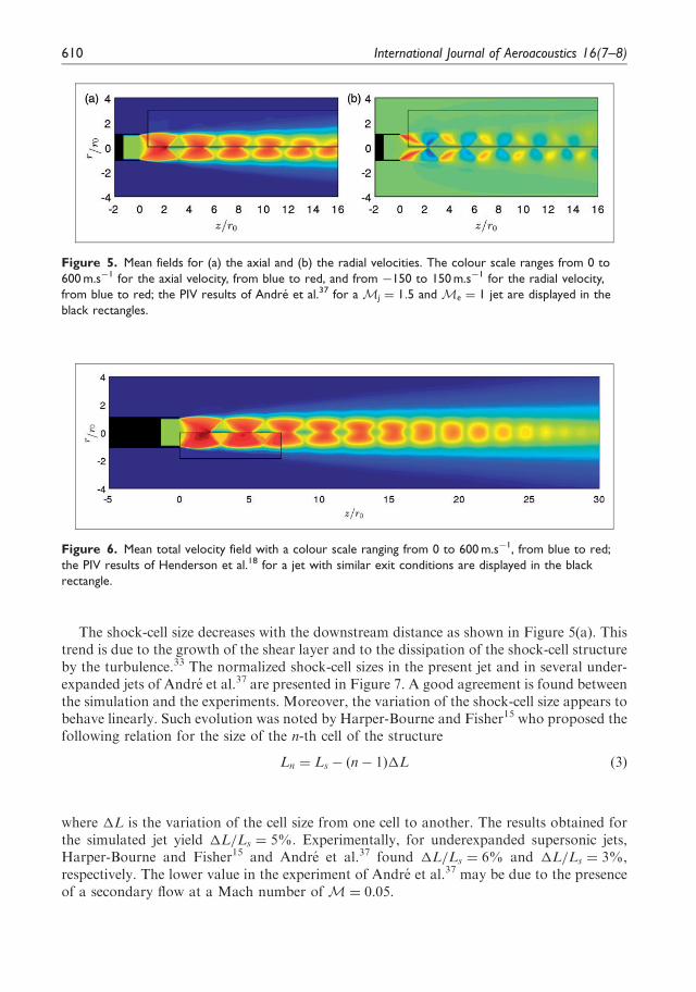
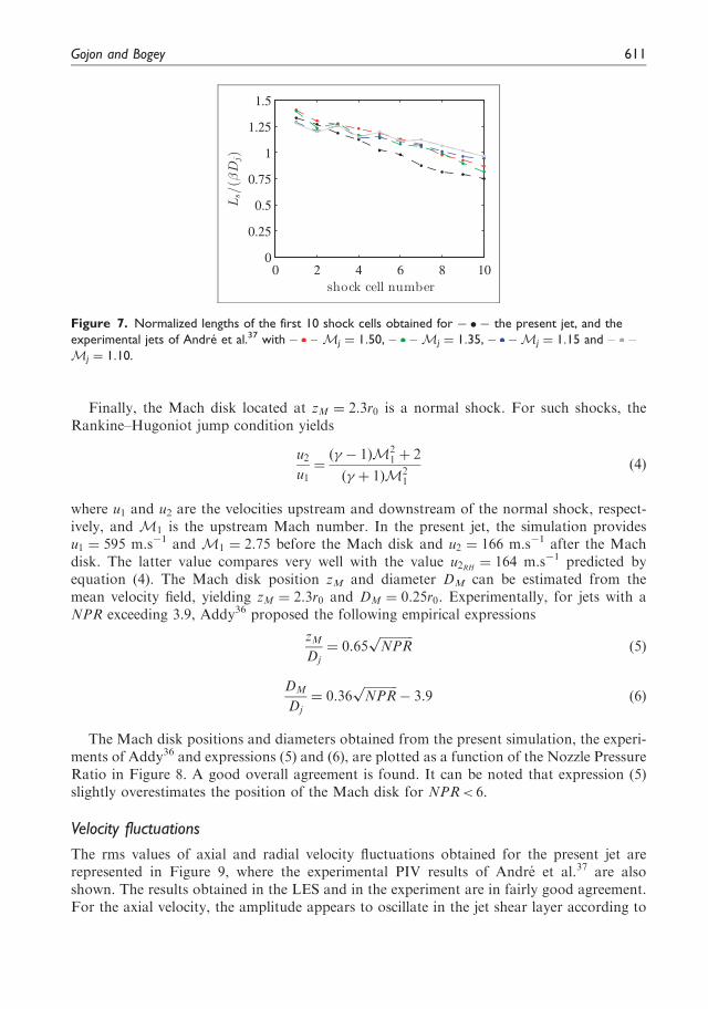
The shock-cell size decreases with the downstream distance as shown in Figure 5(a). Thistrend is due to the growth of the shear layer and to the dissipation of the shock-cell structureby the turbulence.33 The normalized shock-cell sizes in the present jet and in several under-expanded jets of Andre et al.37 are presented in Figure 7. A good agreement is found betweenthe simulation and the experiments. Moreover, the variation of the shock-cell size appears tobehave linearly. Such evolution was noted by Harper-Bourne and Fisher15 who proposed thefollowing relation for the size of the n-th cell of the structure

Ln ¼ Ls � ðn� 1Þ�L ð3Þ

where �L is the variation of the cell size from one cell to another. The results obtained forthe simulated jet yield �L=Ls ¼ 5%. Experimentally, for underexpanded supersonic jets,Harper-Bourne and Fisher15 and Andre et al.37 found �L=Ls ¼ 6% and �L=Ls ¼ 3%,respectively. The lower value in the experiment of Andre et al.37 may be due to the presenceof a secondary flow at a Mach number ofM¼ 0:05.

Figure 5. Mean fields for (a) the axial and (b) the radial velocities. The colour scale ranges from 0 to

600 m.s�1 for the axial velocity, from blue to red, and from �150 to 150 m.s�1 for the radial velocity,

from blue to red; the PIV results of Andre et al.37 for aMj ¼ 1:5 andMe ¼ 1 jet are displayed in the

black rectangles.

Figure 6. Mean total velocity field with a colour scale ranging from 0 to 600 m.s�1, from blue to red;

the PIV results of Henderson et al.18 for a jet with similar exit conditions are displayed in the black

rectangle.


Finally, the Mach disk located at zM ¼ 2:3r0 is a normal shock. For such shocks, theRankine–Hugoniot jump condition yields

u2u1¼ð� � 1ÞM2

1 þ 2

ð� þ 1ÞM21

ð4Þ

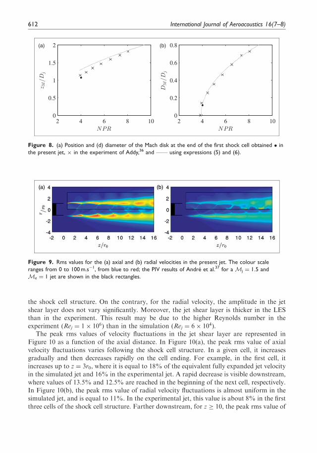
where u1 and u2 are the velocities upstream and downstream of the normal shock, respect-ively, and M1 is the upstream Mach number. In the present jet, the simulation providesu1 ¼ 595 m.s�1 and M1 ¼ 2:75 before the Mach disk and u2 ¼ 166 m.s�1 after the Machdisk. The latter value compares very well with the value u2RH ¼ 164 m.s�1 predicted byequation (4). The Mach disk position zM and diameter DM can be estimated from themean velocity field, yielding zM ¼ 2:3r0 and DM ¼ 0:25r0. Experimentally, for jets with aNPR exceeding 3.9, Addy36 proposed the following empirical expressions

zMDj¼ 0:65

ffiffiffiffiffiffiffiffiffiffiffiNPRp

ð5Þ

DM

Dj¼ 0:36

ffiffiffiffiffiffiffiffiffiffiffiNPRp

� 3:9 ð6Þ

The Mach disk positions and diameters obtained from the present simulation, the experi-ments of Addy36 and expressions (5) and (6), are plotted as a function of the Nozzle PressureRatio in Figure 8. A good overall agreement is found. It can be noted that expression (5)slightly overestimates the position of the Mach disk for NPR< 6.

Velocity fluctuations

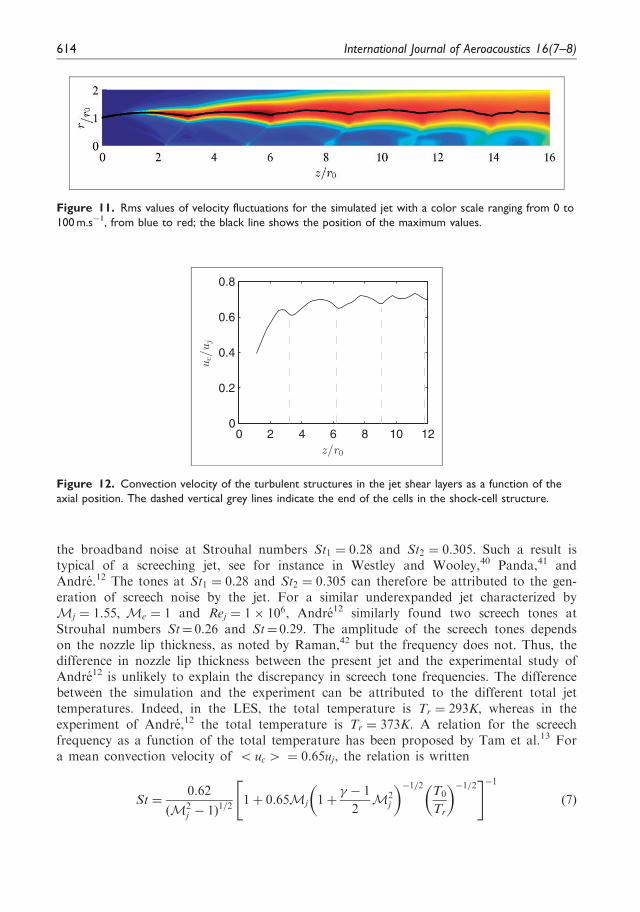
The rms values of axial and radial velocity fluctuations obtained for the present jet arerepresented in Figure 9, where the experimental PIV results of Andre et al.37 are alsoshown. The results obtained in the LES and in the experiment are in fairly good agreement.For the axial velocity, the amplitude appears to oscillate in the jet shear layer according to

0 2 4 6 8 100

0.25

0.5

0.75

1

1.25

1.5

shock cell number

Ls/(β

Dj)

Figure 7. Normalized lengths of the first 10 shock cells obtained for � � � the present jet, and the

experimental jets of Andre et al.37 with Mj ¼ 1:50, Mj ¼ 1:35, Mj ¼ 1:15 and

Mj ¼ 1:10.

Gojon and Bogey 611

the shock cell structure. On the contrary, for the radial velocity, the amplitude in the jet

shear layer does not vary significantly. Moreover, the jet shear layer is thicker in the LES

than in the experiment. This result may be due to the higher Reynolds number in the

experiment (Rej ¼ 1� 106) than in the simulation (Rej ¼ 6� 104).The peak rms values of velocity fluctuations in the jet shear layer are represented in

Figure 10 as a function of the axial distance. In Figure 10(a), the peak rms value of axial

velocity fluctuations varies following the shock cell structure. In a given cell, it increases

gradually and then decreases rapidly on the cell ending. For example, in the first cell, it

increases up to z ¼ 3r0, where it is equal to 18% of the equivalent fully expanded jet velocity

in the simulated jet and 16% in the experimental jet. A rapid decrease is visible downstream,

where values of 13.5% and 12.5% are reached in the beginning of the next cell, respectively.

In Figure 10(b), the peak rms value of radial velocity fluctuations is almost uniform in the

simulated jet, and is equal to 11%. In the experimental jet, this value is about 8% in the first

three cells of the shock cell structure. Farther downstream, for z � 10, the peak rms value of

2 4 6 8 100

0.5

1

1.5

2

NPR

z M/D

j(a)

2 4 6 8 100

0.2

0.4

0.6

0.8

NPR

DM

/D

j

(b)

Figure 8. (a) Position and (d) diameter of the Mach disk at the end of the first shock cell obtained � in

the present jet, � in the experiment of Addy,36 and using expressions (5) and (6).

Figure 9. Rms values for the (a) axial and (b) radial velocities in the present jet. The colour scale

ranges from 0 to 100 m.s�1, from blue to red; the PIV results of Andre et al.37 for aMj ¼ 1:5 and

Me ¼ 1 jet are shown in the black rectangles.


radial velocity fluctuations varies according to the shock cell structure in the experimentaljet.

Convection velocity

The local convection velocity of the turbulent structures is estimated at the center of theshear layer, where the velocity fluctuations are maximum, as presented in Figure 11. It iscalculated from cross-correlations of axial velocity fluctuations between two points locatedat z� 0:1r0.

The local convection velocity obtained in the present jet is presented in Figure 12 as afunction of the axial direction. It is not constant but varies according to the shock-cellstructure, as observed experimentally by Andre12 for round underexpanded jets. In thefirst cell, for example, the convection velocity increases from the value uc ¼ 0:4uj up tothe value 0:63uj, as the velocity inside the jet increases. Farther downstream, the convectionvelocity decreases down to the value of 0:60uj, following the decrease of the velocity insidethe jet due to the presence of a Mach disk and of an oblique annular shock. Similar vari-ations are found for the other cells of the shock cell structure. Furthermore, the convectionvelocity is close to the value 0:35uj ’ 0:5ue at the nozzle exit, as expected for instabilitiesinitially growing in the mixing layers just downstream of the nozzle. Moreover, the convec-tion velocity tends to the value uc ¼ 0:65uj several radii downstream of the nozzle. This resultis in agreement with the experimental results of Harper-Bourne and Fisher,15 who found aconvection velocity of uc ’ 0:70uj for underexpanded supersonic jets using a crossed beamschlieren technique.

Acoustic results

Acoustic spectrum near the nozzle exit

The pressure spectrum obtained near the nozzle exit at z¼ 0 and r ¼ 2r0 is displayed inFigure 13 as a function of the Strouhal number St ¼ fDj=uj. Two tones emerge 15 dB above

0 2 4 6 8 10 12 14 160

0.05

0.1

0.15

0.2

z/r0

<u

zu

z>

1/2

/u

j(a)

0 2 4 6 8 10 12 14 160

0.05

0.1

0.15

0.2

z/r0

<u

ru

r>

1/2

/u

j

(b)

Figure 10. Peak rms values of (a) axial and (b) radial velocity fluctuations as a function of the axial pos-

ition; —— simulation results and – – – PIV results of Andre et al.37 for aMj ¼ 1:5 andMe ¼ 1 jet. The

dashed vertical grey lines indicate the end of the cells in the shock-cell structure of the simulated jet.

Gojon and Bogey 613

the broadband noise at Strouhal numbers St1 ¼ 0:28 and St2 ¼ 0:305. Such a result istypical of a screeching jet, see for instance in Westley and Wooley,40 Panda,41 andAndre.12 The tones at St1 ¼ 0:28 and St2 ¼ 0:305 can therefore be attributed to the gen-eration of screech noise by the jet. For a similar underexpanded jet characterized byMj ¼ 1:55, Me ¼ 1 and Rej ¼ 1� 106, Andre12 similarly found two screech tones atStrouhal numbers St¼ 0.26 and St¼ 0.29. The amplitude of the screech tones dependson the nozzle lip thickness, as noted by Raman,42 but the frequency does not. Thus, thedifference in nozzle lip thickness between the present jet and the experimental study ofAndre12 is unlikely to explain the discrepancy in screech tone frequencies. The differencebetween the simulation and the experiment can be attributed to the different total jettemperatures. Indeed, in the LES, the total temperature is Tr ¼ 293K, whereas in theexperiment of Andre,12 the total temperature is Tr ¼ 373K. A relation for the screechfrequency as a function of the total temperature has been proposed by Tam et al.13 Fora mean convection velocity of 5 uc 4 ¼ 0:65uj, the relation is written

St ¼0:62

ðM2j � 1Þ1=2

1þ 0:65Mj 1þ� � 1

2M

2j

� ��1=2T0

Tr

� ��1=2" #�1ð7Þ

0 2 4 6 8 10 120

0.2

0.4

0.6

0.8

z/r0

uc/

uj

Figure 12. Convection velocity of the turbulent structures in the jet shear layers as a function of the

axial position. The dashed vertical grey lines indicate the end of the cells in the shock-cell structure.

Figure 11. Rms values of velocity fluctuations for the simulated jet with a color scale ranging from 0 to

100 m.s�1, from blue to red; the black line shows the position of the maximum values.


Equation (7) gives St¼ 0.285 for the simulated jet and St¼ 0.265 for the experimental jet,

supporting that the difference in screech frequencies between the LES and the experiment is

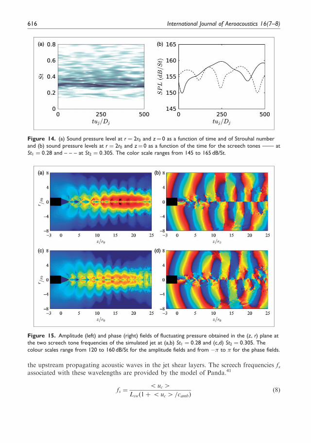
related to the total temperature of the jet.In order to determine whether the jet products alternatively or simultaneously the two

screech tones obtained in the spectrum of Figure 13, a Fast Fourier transform is applied

using a sliding window in time, of size 35uj=Dj. The result is displayed in Figure 14(a) where

the sound pressure level is represented as a function of time tuj=Dj and Strouhal number. The

two screech frequencies at St1 ¼ 0:28 and St2 ¼ 0:305 are visible but their amplitudes vary in

time. The sound pressure levels obtained for the two screech tones are shown in Figure 14(b)

as a function of time. The intensities of the two tones oscillate between 125 dB/St and

135 dB/St. Moreover, it appears that when the intensity of one screech tone is weak, the

intensity of the other tone is strong. A switch between these two tones is thus observed. For

non-ideally expanded jets exiting from a rectangular nozzle with a single-bevelled exit,

Raman43 also observed two screech tones switching in time.

Fluctuating pressure in the jet

The pressure fields in the (z, r) plane have been recorded every 50th time step. A Fourier

transform then is applied on each point of the (z, r) plane. In this way, for a given frequency,

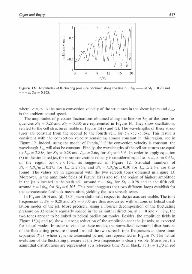
the amplitude and the phase fields can be shown. For the screech tones at St1 ¼ 0:28 and

St2 ¼ 0:305, they are given in Figure 15. The amplitude fields in Figure 15(a) and (c) exhibit

different cell structures. The structures are due to the formation of hydrodynamic-acoustic

standing waves. Such waves were previously observed in supersonic screeching jets experi-

mentally by Panda41 by examining the root-mean-square values of pressure fluctuations in

the near field and numerically by Gojon and Bogey.44 They were also observed by Gojon

et al.45 and Bogey and Gojon46 in ideally-expanded impinging jets by applying Fourier

decomposition to the mean pressure fields and looking at the amplitude fields at the tone

frequencies. The cell lengths in these structures are equal to the wavelengths Lsw of the

standing waves formed between the downstream propagating hydrodynamic waves and

St = fDj/uj

10 -1 10 0

SP

L(d

B/S

t)120

130

140

150

160

Figure 13. Pressure spectrum at r ¼ 2r0 and z¼ 0 as a function of the Strouhal number.

Gojon and Bogey 615

the upstream propagating acoustic waves in the jet shear layers. The screech frequencies fsassociated with these wavelengths are provided by the model of Panda.41

fs ¼5 uc4

Lswð1þ 5 uc 4 =cambÞð8Þ

Figure 15. Amplitude (left) and phase (right) fields of fluctuating pressure obtained in the (z, r) plane at

the two screech tone frequencies of the simulated jet at (a,b) St1 ¼ 0:28 and (c,d) St2 ¼ 0:305. The

colour scales range from 120 to 160 dB/St for the amplitude fields and from �� to � for the phase fields.

Figure 14. (a) Sound pressure level at r ¼ 2r0 and z¼ 0 as a function of time and of Strouhal number

and (b) sound pressure levels at r ¼ 2r0 and z¼ 0 as a function of the time for the screech tones —— at

St1 ¼ 0:28 and – – – at St2 ¼ 0:305. The color scale ranges from 145 to 165 dB/St.


where 5 uc 4 is the mean convection velocity of the structures in the shear layers and camb

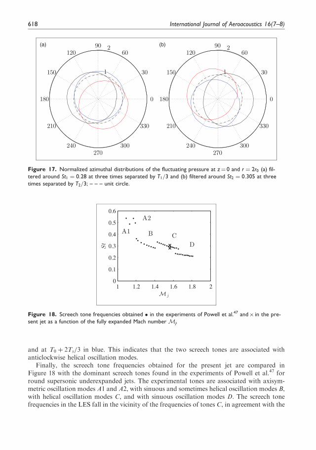
is the ambient sound speed.The amplitudes of pressure fluctuations obtained along the line r ¼ 3r0 at the tone fre-

quencies St1 ¼ 0:28 and St2 ¼ 0:305 are represented in Figure 16. They show oscillations,

related to the cell structures visible in Figure 15(a) and (c). The wavelengths of these struc-

tures are constant from the second to the fourth cell, for 5r0 5 z5 15r0. This result is

consistent with the convection velocity remaining almost constant in this region, see in

Figure 12. Indeed, using the model of Panda,41 if the convection velocity is constant, the

wavelength Lsw will also be constant. Finally, the wavelengths of the cell structures are equal

to Lsw ’ 2:85r0 for St1 ¼ 0:28 and Lsw ’ 2:6r0 for St2 ¼ 0:305. In order to apply equation

(8) to the simulated jet, the mean convection velocity is considered equal to 5 uc 4 ¼ 0:65ujin the region 5r0 5 z5 15r0, as suggested in Figure 12. Strouhal numbers of

Sts ¼ fsDj=uj ’ 0:275 for Lsw ’ 2:85r0 and Sts ¼ fsDj=uj ’ 0:30 for Lsw ’ 2:6r0 are thus

found. The values are in agreement with the two screech tones obtained in Figure 13.

Moreover, in the amplitude fields of Figure 15(a) and (c), the region of highest amplitude

in the jet is located in the sixth cell, around z ¼ 16r0, for St1 ¼ 0:28 and in the fifth cell,

around z ¼ 14r0, for St2 ¼ 0:305. This result suggests that two different loops establish for

the aeroacoustic feedback mechanism, yielding the two screech tones.In Figure 15(b) and (d), 180� phase shifts with respect to the jet axis are visible. The tone

frequencies at St1 ¼ 0:28 and St2 ¼ 0:305 are thus associated with sinuous or helical oscil-

lation modes of the jet. More precisely, using a Fourier decomposition of the fluctuating

pressure on 32 sensors regularly spaced in the azimuthal direction, at z¼ 0 and r ¼ 2r0, the

two tones appear to be linked to helical oscillation modes. Besides, the amplitude fields in

Figure 15(a) and (c) show a strong reduction of the amplitude near the jet axis, as expected

for helical modes. In order to visualize these modes, the normalized azimuthal distributions

of the fluctuating pressure filtered around the two screech tone frequencies at three times

separated Ts=3, where Ts is the associated period, are represented in Figure 17. The helical

evolution of the fluctuating pressure at the two frequencies is clearly visible. Moreover, the

azimuthal distributions are represented at a reference time T0 in black, at T0 þ Ts=3 in red

0 4 8 12 16 20−1

−0.5

0

0.5

1

z/r0

arbit

rary

unit

Figure 16. Amplitudes of fluctuating pressure obtained along the line r ¼ 3r0 —— at St1 ¼ 0:28 and

– – – at St2 ¼ 0:305.

Gojon and Bogey 617

and at T0 þ 2Ts=3 in blue. This indicates that the two screech tones are associated withanticlockwise helical oscillation modes.

Finally, the screech tone frequencies obtained for the present jet are compared inFigure 18 with the dominant screech tones found in the experiments of Powell et al.47 forround supersonic underexpanded jets. The experimental tones are associated with axisym-metric oscillation modes A1 and A2, with sinuous and sometimes helical oscillation modes B,with helical oscillation modes C, and with sinuous oscillation modes D. The screech tonefrequencies in the LES fall in the vicinity of the frequencies of tones C, in agreement with the

1

2

30

210

60

240

90

270

120

300

150

330

180 0

(a)

1

2

30

210

60

240

90

270

120

300

150

330

180 0

(b)

Figure 17. Normalized azimuthal distributions of the fluctuating pressure at z¼ 0 and r ¼ 2r0 (a) fil-

tered around St1 ¼ 0:28 at three times separated by T1=3 and (b) filtered around St2 ¼ 0:305 at three

times separated by T2=3; – – – unit circle.

1 1.2 1.4 1.6 1.8 20

0.1

0.2

0.3

0.4

0.5

0.6

M j

St

A1

A2

B CD

Figure 18. Screech tone frequencies obtained � in the experiments of Powell et al.47 and� in the pre-

sent jet as a function of the fully expanded Mach numberMj.


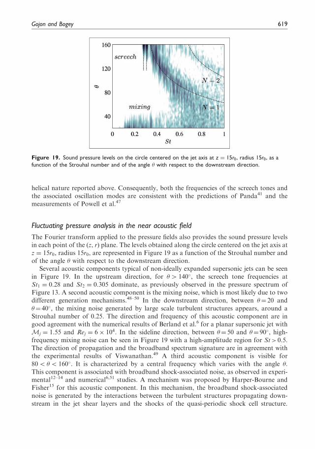
helical nature reported above. Consequently, both the frequencies of the screech tones andthe associated oscillation modes are consistent with the predictions of Panda41 and themeasurements of Powell et al.47

Fluctuating pressure analysis in the near acoustic field

The Fourier transform applied to the pressure fields also provides the sound pressure levelsin each point of the (z, r) plane. The levels obtained along the circle centered on the jet axis atz ¼ 15r0, radius 15r0, are represented in Figure 19 as a function of the Strouhal number andof the angle � with respect to the downstream direction.

Several acoustic components typical of non-ideally expanded supersonic jets can be seenin Figure 19. In the upstream direction, for �4 140�, the screech tone frequencies atSt1 ¼ 0:28 and St2 ¼ 0:305 dominate, as previously observed in the pressure spectrum ofFigure 13. A second acoustic component is the mixing noise, which is most likely due to twodifferent generation mechanisms.48–50 In the downstream direction, between �¼ 20 and�¼ 40�, the mixing noise generated by large scale turbulent structures appears, around aStrouhal number of 0.25. The direction and frequency of this acoustic component are ingood agreement with the numerical results of Berland et al.6 for a planar supersonic jet withMj ¼ 1:55 and Rej ¼ 6� 104. In the sideline direction, between �¼ 50 and �¼ 90�, high-frequency mixing noise can be seen in Figure 19 with a high-amplitude region for St> 0.5.The direction of propagation and the broadband spectrum signature are in agreement withthe experimental results of Viswanathan.49 A third acoustic component is visible for805 �5 160�. It is characterized by a central frequency which varies with the angle �.This component is associated with broadband shock-associated noise, as observed in experi-mental12–14 and numerical6,51 studies. A mechanism was proposed by Harper-Bourne andFisher15 for this acoustic component. In this mechanism, the broadband shock-associatednoise is generated by the interactions between the turbulent structures propagating down-stream in the jet shear layers and the shocks of the quasi-periodic shock cell structure.

Figure 19. Sound pressure levels on the circle centered on the jet axis at z ¼ 15r0, radius 15r0, as a

function of the Strouhal number and of the angle � with respect to the downstream direction.

Gojon and Bogey 619

Each interaction is considered as an acoustic source. The directivity of constructive inter-ference is then determined. This model yields a central frequency

fshock ¼Nuc

Lsð1�Mc cosð�ÞÞð9Þ

where N is the mode number, Ls is a length scale related to the shock cell size, andMc ¼ uc=camb is the convection Mach number. As the cell length varies with the axial dir-ection, as observed in the Mean fields section, it is difficult to choose the value of Ls. Forscreeching jets, Tam et al.13 suggested that the central frequency of the first mode N¼ 1 ofthe broadband shock-associated noise tends to the screech frequency at �¼ 180�.Considering equation (8), the length scale Ls in equation (9) can therefore be replaced bythe wavelengths of the standing waves Lsw. Unfortunately, the screech frequencies predictedin this way using the two wavelengths Lsw ¼ 2:85r0 and Lsw ¼ 2:6r0 found in the Fluctuatingpressure in the jet section are not in good agreement with the LES results. Harper-Bourneand Fisher15 proposed a mean length of Ls ¼ 1:1�Dj ¼ 2:9r0 for the shock cell structure butthe comparison with the LES results was again not satisfactory. Finally, the size of the sixthshock cell, Ls6 ¼ 2:35r0, located around z ¼ 15r0, is used in the relation (9) to compute thecentral frequency of the broadband shock-associated noise as a function of angle �. Thefrequencies of the modes N¼ 1 and N¼ 2 thus obtained are plotted in Figure 19. There is agood agreement with numerical results. One can finally note that in the upstream direction,the relation (9) tends to St¼ 0.33. This tone can be observed in the spectrum of Figure 13 ata magnitude of 147 dB, comforting the choice of this length scale.

Mixing noise

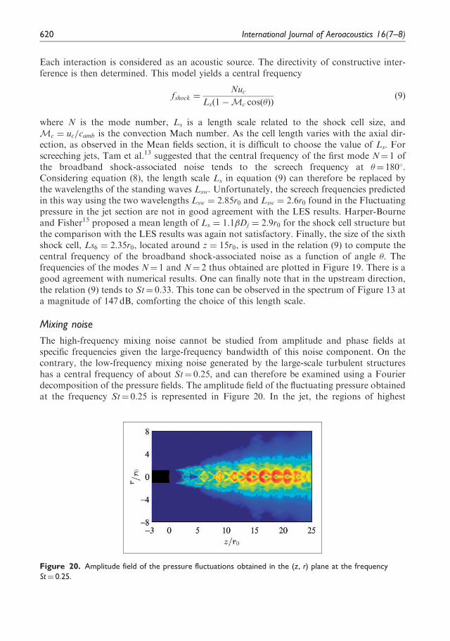
The high-frequency mixing noise cannot be studied from amplitude and phase fields atspecific frequencies given the large-frequency bandwidth of this noise component. On thecontrary, the low-frequency mixing noise generated by the large-scale turbulent structureshas a central frequency of about St¼ 0.25, and can therefore be examined using a Fourierdecomposition of the pressure fields. The amplitude field of the fluctuating pressure obtainedat the frequency St¼ 0.25 is represented in Figure 20. In the jet, the regions of highest

Figure 20. Amplitude field of the pressure fluctuations obtained in the (z, r) plane at the frequency

St¼ 0.25.


amplitude are located in the sixth cell, around z ¼ 15r0. Therefore, the mixing noise seems tobe produced at the end of the potential core, as observed by Bogey and Baily,7 Sandham andSalgado8 and Tam9 for instance.

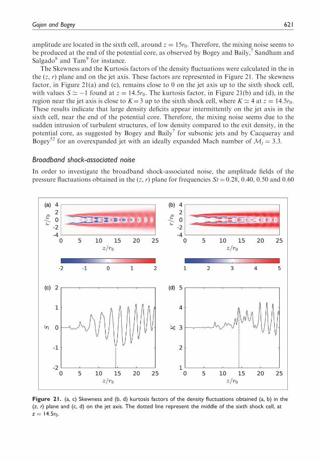
The Skewness and the Kurtosis factors of the density fluctuations were calculated in the inthe (z, r) plane and on the jet axis. These factors are represented in Figure 21. The skewnessfactor, in Figure 21(a) and (c), remains close to 0 on the jet axis up to the sixth shock cell,with values S ’ �1 found at z ¼ 14:5r0. The kurtosis factor, in Figure 21(b) and (d), in theregion near the jet axis is close to K¼ 3 up to the sixth shock cell, where K ’ 4 at z ¼ 14:5r0.These results indicate that large density deficits appear intermittently on the jet axis in thesixth cell, near the end of the potential core. Therefore, the mixing noise seems due to thesudden intrusion of turbulent structures, of low density compared to the exit density, in thepotential core, as suggested by Bogey and Baily7 for subsonic jets and by Cacqueray andBogey52 for an overexpanded jet with an ideally expanded Mach number ofMj ¼ 3:3.

Broadband shock-associated noise

In order to investigate the broadband shock-associated noise, the amplitude fields of thepressure fluctuations obtained in the (z, r) plane for frequencies St¼ 0.28, 0.40, 0.50 and 0.60

Figure 21. (a, c) Skewness and (b, d) kurtosis factors of the density fluctuations obtained (a, b) in the

(z, r) plane and (c, d) on the jet axis. The dotted line represent the middle of the sixth shock cell, at

z ¼ 14:5r0.

Gojon and Bogey 621

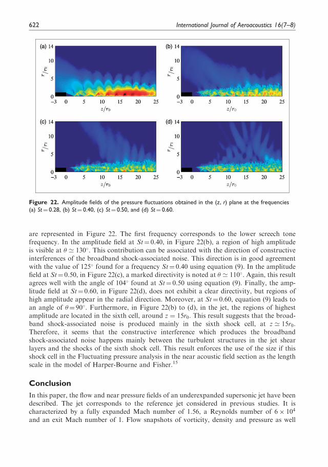
are represented in Figure 22. The first frequency corresponds to the lower screech tonefrequency. In the amplitude field at St¼ 0.40, in Figure 22(b), a region of high amplitudeis visible at � ’ 130�. This contribution can be associated with the direction of constructiveinterferences of the broadband shock-associated noise. This direction is in good agreementwith the value of 125� found for a frequency St¼ 0.40 using equation (9). In the amplitudefield at St¼ 0.50, in Figure 22(c), a marked directivity is noted at � ’ 110�. Again, this resultagrees well with the angle of 104� found at St¼ 0.50 using equation (9). Finally, the amp-litude field at St¼ 0.60, in Figure 22(d), does not exhibit a clear directivity, but regions ofhigh amplitude appear in the radial direction. Moreover, at St¼ 0.60, equation (9) leads toan angle of �¼ 90�. Furthermore, in Figure 22(b) to (d), in the jet, the regions of highestamplitude are located in the sixth cell, around z ¼ 15r0. This result suggests that the broad-band shock-associated noise is produced mainly in the sixth shock cell, at z ’ 15r0.Therefore, it seems that the constructive interference which produces the broadbandshock-associated noise happens mainly between the turbulent structures in the jet shearlayers and the shocks of the sixth shock cell. This result enforces the use of the size if thisshock cell in the Fluctuating pressure analysis in the near acoustic field section as the lengthscale in the model of Harper-Bourne and Fisher.15

Conclusion

In this paper, the flow and near pressure fields of an underexpanded supersonic jet have beendescribed. The jet corresponds to the reference jet considered in previous studies. It ischaracterized by a fully expanded Mach number of 1.56, a Reynolds number of 6� 104

and an exit Mach number of 1. Flow snapshots of vorticity, density and pressure as well

Figure 22. Amplitude fields of the pressure fluctuations obtained in the (z, r) plane at the frequencies

(a) St¼ 0.28, (b) St¼ 0.40, (c) St¼ 0.50, and (d) St¼ 0.60.


as mean velocity fields are shown. The results, including the shock-cell structure, are con-sistent with experimental data, empirical and theoretical models. The convection velocity oflarge-scale structures in the jet shear layers is evaluated, and values similar to experimentaldata are found. The near acoustic pressure fields are then analyzed. Two tone frequenciesassociated with screech noise are obtained in the acoustic spectrum calculated in the vicinityof the nozzle. Hydrodynamic-acoustic standing waves, typical of this noise component, areobserved. The two screech tones are found to be associated with anticlockwise helical oscil-lation modes. Moreover, a temporal switch between the two screech tone frequencies isnoted. Then in the near pressure fields, the low-frequency mixing noise, the high-frequencymixing noise and the broadband shock-associated noise are identified. They are found to beproduced mainly in the sixth shock cell. The mixing noise component seems due to thesudden intrusion of turbulent structures into the potential core, near its end. The broadbandshock-associated noise appears to originate from the interactions between the turbulentstructures in the jet shear layers and the shocks of the sixth shock cell. The use of the sizeof this shock cell in the classical theoretical model of this noise component is proposed and agood agreement is found with simulation results.

Acknowledgements

This work was granted access to the HPC resources of FLMSN (Federation Lyonnaise de

Modelisation et Sciences Numeriques), partner of EQUIPEX EQUIP@MESO, and of CINES

(Centre Informatique National de l’Enseignement Superieur), and IDRIS (Institut du

Developpement et des Ressources en Informatique Scientifique) under the allocation 2016-2a0204

made by GENCI (Grand Equipement National de Calcul Intensif).

Declaration of conflicting interests

The author(s) declared no potential conflicts of interest with respect to the research, authorship, and/or

publication of this article.

Funding

The author(s) disclosed receipt of the following financial support for the research, authorship, and/or

publication of this article: This work was performed within the framework of the Labex CeLyA of

Universite de Lyon, operated by the French National Research Agency (grant no. ANR-10-LABX-

0060/ANR-11-IDEX-0007).

References

1. Powell A. On the mechanism of choked jet noise. Proc Physical Soc Sect B 1953; 66: 1039–1056.

2. Raman G. Supersonic jet screech: half-century from Powell to the present. J Sound Vib 1999; 225:

543–571.3. Merle M. Sur la frequence des ondes sonores emises par un jet d’air a grande vitesse. Comptes-

Rendus de l’Academie des Sciences de Paris 1956; 243: 490–493.4. Davies MG and Oldfield DES. Tones from a choked axisymmetric jet. ii. the self excited loop and

mode of oscillation. Acta Acust United Acust 1962; 12: 267–277.5. Bogey C and Bailly C. Investigation of downstream and sideline subsonic jet noise using large eddy

simulation. Theor Comput Fluid Dyn 2006; 20: 23–40.6. Berland J, Bogey C and Bailly C. Numerical study of screech generation in a planar supersonic jet.

Phys Fluids 2007; 19: 075105.

Gojon and Bogey 623

7. Bogey C and Bailly C. An analysis of the correlations between the turbulent flow and the sound

pressure fields of subsonic jets. J Fluid Mech 2007; 583: 71–97.8. Sandham ND and Salgado AM. Nonlinear interaction model of subsonic jet noise. Phil Trans R

Soc A 2008; 366: 2745–2760.9. Tam CKW. Mach wave radiation from high-speed jets. AIAA J 2009; 47: 2440–2448.

10. Bogey C, Bailly C and Juve D. Noise investigation of a high subsonic, moderate reynolds number

jet using a compressible large eddy simulation. Theoret Comput Fluid Dynam 2003; 16: 273–297.

11. Martlew DL. Noise associated with shock waves in supersonic jets. Aircraft engine noise and sonic

boom. AGARD C.P. 1969; 42: 1–70.

12. Andre B. Etude experimentale de l’effet du vol sur le bruit de choc de jets supersoniques sous-

detendus. PhD Thesis, Ecole Centrale de Lyon, NNT: 2012ECDL0042, 2012.

13. Tam C.K.W., Seiner J.M. and Yu J.C.. Proposed relationship between broadband shock asso-

ciated noise and screech tones. J. Sound Vib. 1986; 110(2): 309–321.

14. Tam CKW and Tanna HK. Shock associated noise of supersonic jets from convergent-divergent

nozzles. J Sound Vib 1982; 81: 337–358.

15. Harper-Bourne M and Fisher MJ. The noise from shock waves in supersonic jets. AGARD CP

1974; 131: 1–13.

16. Gojon R and Bogey C. Flow structure oscillations and tone production in underexpanded imping-

ing round jets. AIAA J 2017; 55: 1–14.

17. Castelain T, Gojon R, Mercier B, et al. Estimation of convection speed in underexpanded jets from

schlieren pictures. AIAA Paper 2016; 2016–2984: 1–14.

18. Henderson B, Bridges J and Wernet M. An experimental study of the oscillatory flow structure of

tone-producing supersonic impinging jets. J Fluid Mech 2005; 542: 115–137.

19. Bogey C, Marsden O and Bailly C. Large-eddy simulation of the flow and acoustic fields of a

Reynolds number 105 subsonic jet with tripped exit boundary layers. Phys Fluid 2011; 23: 1–20.

20. Bogey C and Bailly C. A family of low dispersive and low dissipative explicit schemes for flow and

noise computations. J Comput Phys 2004; 194: 194–214.

21. Berland J, Bogey C, Marsden O, et al. High-order, low dispersive and low dissipative explicit

schemes for multiple-scale and boundary problems. J Comput Phys 2007; 224: 637–662.

22. Bogey C and Bailly C. Large eddy simulations of transitional round jets: influence of the Reynolds

number on flow development and energy dissipation. Phys Fluid 2006; 18: 1–14.

23. Bogey C and Bailly C. Turbulence and energy budget in a self-preserving round jet: direct evalu-

ation using large eddy simulation. J Fluid Mech 2009; 627: 129–160.

24. Fauconnier D, Bogey C and Dick E. On the performance of relaxation filtering for large-eddy

simulation. J Turbul 2013; 14: 22–49.

25. Kremer F and Bogey C. Large-eddy simulation of turbulent channel flow using relaxation filtering:

Resolution requirement and Reynolds number effects. Comput Fluid 2015; 116: 17–28.

26. Tam CKW and Dong Z. Wall boundary conditions for high-order finite-difference schemes in

computational aeroacoustics. Theor Comput Fluid Dynam 1994; 6: 303–322.

27. Bogey C, de Cacqueray N and Bailly C. Finite differences for coarse azimuthal discretization and

for reduction of effective resolution near origin of cylindrical flow equations. J Comput Phys 2011;

230: 1134–1146.28. Mohseni K and Colonius T. Numerical treatment of polar coordinate singularities. J Comput Phys

2000; 157: 787–795.29. Bogey C, de Cacqueray N and Bailly C. A shock-capturing methodology based on adaptative

spatial filtering for high-order non-linear computations. J Comput Phys 2009; 228: 1447–1465.30. de Cacqueray N, Bogey C and Bailly C. Investigation of a high-mach-number overexpanded jet

using large-eddy simulation. AIAA J 2011; 49: 2171–2182.31. Arnette SA, Samimy M and Elliott GS. On streamwise vortices in high Reynolds number super-

sonic axisymmetric jets. Phys Fluids 1993; 5: 187–202.


32. Lau JC, Morris PJ and Fisher MJ. Measurements in subsonic and supersonic free jets using a laser

velocimeter. J Fluid Mech 1979; 93: 1–27.33. Tam CKW, Jackson JA and Seiner JM. A multiple-scales model of the shock-cell structure of

imperfectly expanded supersonic jets. J Fluid Mech 1985; 153: 123–149.

34. Powell A. The sound-producing oscillations of round underexpanded jets impinging on normalplates. J Acoust Soc Am 1988; 83: 515–533.

35. Henderson B. The connection between sound production and jet structure of the supersonicimpinging jet. J Acoust Soc Am 2002; 111: 735–747.

36. Addy AL. Effects of axisymmetric sonic nozzle geometry on mach disk characteristics. AIAA J1981; 19: 121–122.

37. Andre B, Castelain T and Bailly C. Investigation of the mixing layer of underexpanded supersonic

jets by particle image velocimetry. Intl J Heat Fluid Flow 2014; 50: 188–200.38. Prandtl L. Uber die stationren wellen in einem gasstrahl. Physikalische Zeitschrift 1904; 5:

599–601.

39. Pack DC. A note on Prandtl’s formula for the wave-length of a supersonic gas jet. Q J Mech ApplMath 1950; 3: 173–181.

40. Westley R and Woolley JH. The near field sound pressures of a choked jet during a screech cycle.

AGARD CP 1969; 42: 1–23.41. Panda J. An experimental investigation of screech noise generation. J Fluid Mech 1999; 378: 71–96.42. Raman G. Cessation of screech in underexpanded jets. J Fluid Mech 1997; 336: 69–90.43. Raman G. Screech tones from rectangular jets with spanwise oblique shock-cell structures. J. Fluid

Mech 1997; 330: 141–168.44. Gojon R and Bogey C. On the oscillation modes in screeching jets. AIAA J 2017; submitted.45. Gojon R, Bogey C and Marsden O. Investigation of tone generation in ideally expanded super-

sonic planar impinging jets using large-eddy simulation. J Fluid Mech 2016; 808: 90–115.46. Bogey C and Gojon R. Feedback loop and upwind-propagating waves in ideally-expanded super-

sonic impinging round jets. J Fluid Mech 2017; 823: 562–591.

47. Powell A, Umeda Y and Ishii R. Observations of the oscillation modes of choked circular jets.J Acoust Soc Am 1992; 92: 2823–2836.

48. Tam CKW, Golebiowski M and Seiner JM. On the two components of turbulent mixing noise

from supersonic jets. AIAA Paper 1996; 1996–1716: 1–11.49. Viswanathan K. Analysis of the two similarity components of turbulent mixing noise. AIAA J

2002; 40: 1735–1744.50. Tam CKW, Viswanathan K, Ahuja KK, et al. The sources of jet noise: experimental evidence.

J Fluid Mech 2008; 615: 253–292.51. Dahl MD. Predictions of supersonic jet mixing and shock-associated noise compared with mea-

sured far-field data. NASA Technical Report, TM-2010-216328, 2010.

52. de Cacqueray N and Bogey C. Noise of an overexpanded mach 3.3 jet: non-linear propagationeffects and correlations with flow. Int J Aeroacoust 2014; 13: 607–632.

Gojon and Bogey 625

journals.sagepub.com/home/jae free jet generating two ...

Documents

Transcript of journals.sagepub.com/home/jae free jet generating two ...