𝜋: ESTIMATES, CONFIDENCE INTERVALS, AND TESTS

Business Statistics

The CLT for 𝜋Estimating proportion

Hypothesis on the proportion

Old exam question

Further study

CONTENTS

▪ Estimating, confidence intervals, and hypothesis test for 𝜇are based on the central limit theorem▪ and therefore on the normal distribution

▪ For 𝜎2 we needed another distribution▪ the 𝜒2-distribution

▪ What to use for 𝜋?▪ the probability of success in a Bernoulli experiment

▪ Based on sampling theory▪ so, repeated Bernoulli experiment

▪ so, a binomial distribution

▪ and for large 𝑛, approximately a normal distribution (→ CLT)

THE CLT FOR 𝜋

Define 𝑋𝑖 as the outcome (0 or 1) in one Bernoulli experiment

▪ Total number of “1”s in 𝑛 Bernoulli experiments▪ 𝑌 = σ𝑖=1

𝑛 𝑋𝑖▪ Average number of “1”s (due to CLT, with binomial results):

▪ 𝑃 =𝑌

𝑛= ത𝑋~𝑁 𝜇𝑋,

𝜎𝑋2

𝑛= 𝑁 𝜋,

𝜋 1−𝜋

𝑛

▪ provided 𝑛𝜋 ≥ 5 and 𝑛 1 − 𝜋 ≥ 5

THE CLT FOR 𝜋

𝑃 is the estimator of 𝜋a concrete estimate is 𝑝

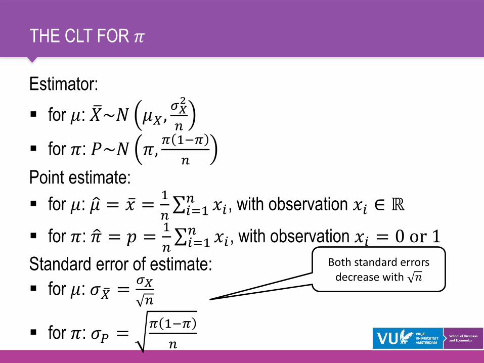
Estimator:

▪ for 𝜇: ത𝑋~𝑁 𝜇𝑋,𝜎𝑋2

𝑛

▪ for 𝜋: 𝑃~𝑁 𝜋,𝜋 1−𝜋

𝑛

Point estimate:

▪ for 𝜇: ො𝜇 = ҧ𝑥 =1

𝑛σ𝑖=1𝑛 𝑥𝑖, with observation 𝑥𝑖 ∈ ℝ

▪ for 𝜋: ො𝜋 = 𝑝 =1

𝑛σ𝑖=1𝑛 𝑥𝑖, with observation 𝑥𝑖 = 0 or 1

Standard error of estimate:

▪ for 𝜇: 𝜎 ത𝑋 =𝜎𝑋

𝑛

▪ for 𝜋: 𝜎𝑃 =𝜋 1−𝜋

𝑛

THE CLT FOR 𝜋

Both standard errors decrease with 𝑛

▪ Estimating 𝜋 by 𝑝

▪ and estimating 𝜎𝑃 =𝜋 1−𝜋

𝑛by 𝑠𝑃 =

𝑝 1−𝑝

𝑛

▪ standard error of proportion

▪ So, we have for 𝜋▪ a point estimate 𝑝 =

𝑌

𝑛

▪ an interval estimate 𝑝 − 𝑧𝛼/2𝑝 1−𝑝

𝑛, 𝑝 + 𝑧𝛼/2

𝑝 1−𝑝

𝑛

▪ 1 − 𝛼 confidence interval for 𝜋

▪ 𝑝 − 𝑧𝛼/2𝑝 1−𝑝

𝑛≤ 𝜋 ≤ 𝑝 + 𝑧𝛼/2

𝑝 1−𝑝

𝑛

ESTIMATING PROPORTION

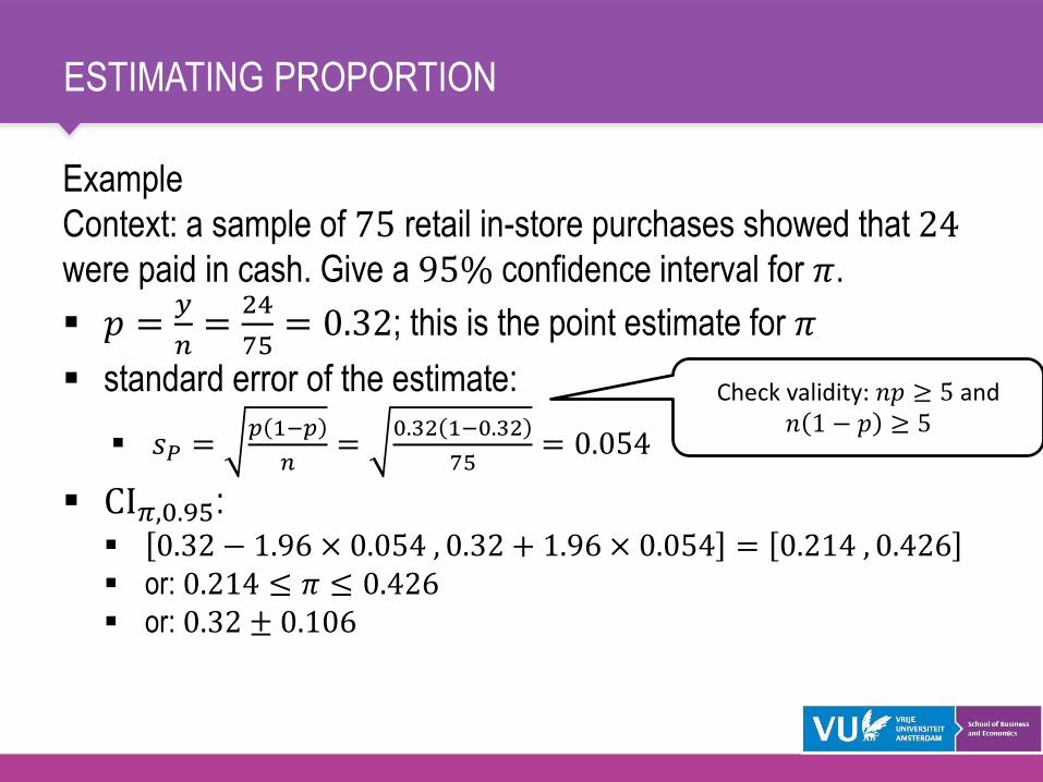
Example

Context: a sample of 75 retail in-store purchases showed that 24were paid in cash. Give a 95% confidence interval for 𝜋.

▪ 𝑝 =𝑦

𝑛=

24

75= 0.32; this is the point estimate for 𝜋

▪ standard error of the estimate:

▪ 𝑠𝑃 =𝑝 1−𝑝

𝑛=

0.32 1−0.32

75= 0.054

▪ CI𝜋,0.95: ▪ 0.32 − 1.96 × 0.054 , 0.32 + 1.96 × 0.054 = 0.214 , 0.426▪ or: 0.214 ≤ 𝜋 ≤ 0.426▪ or: 0.32 ± 0.106

ESTIMATING PROPORTION

Check validity: 𝑛𝑝 ≥ 5 and 𝑛 1 − 𝑝 ≥ 5

You flip a coin 100 times and find 45 times head. Give a

95% confidence interval for 𝜋ℎ𝑒𝑎𝑑 .

EXERCISE 1

Test a hypothesis on the proportion of a Bernoulli process

▪ Example:▪ you are a police officer

▪ you wonder if less than 50% of the (one-sided) traffic accidents

occur with female drivers driving the car

HYPOTHESES ON THE PROPORTION

▪ Statistical model▪ each accident has an underlying Bernouilli process of happening

to a man (0) or to a woman (1), 𝑋~𝑎𝑙𝑡 𝜋▪ you observe the next 𝑛 = 5 car accidents, and report the

outcomes (0/1)

▪ you define 𝑌 as the number of accidents that is caused by a

woman

▪ the sequence of 5 observations can be regarded as a binomial

process, 𝑌~𝐵𝑖𝑛 𝜋, 5▪ you start by assuming the accident rates are equal, i.e.,

hypothesize that 𝜋 = 0.5

▪ Suppose you observed 𝑦 = 1, i.e., one car accident by a

woman

HYPOTHESES ON THE PROPORTION

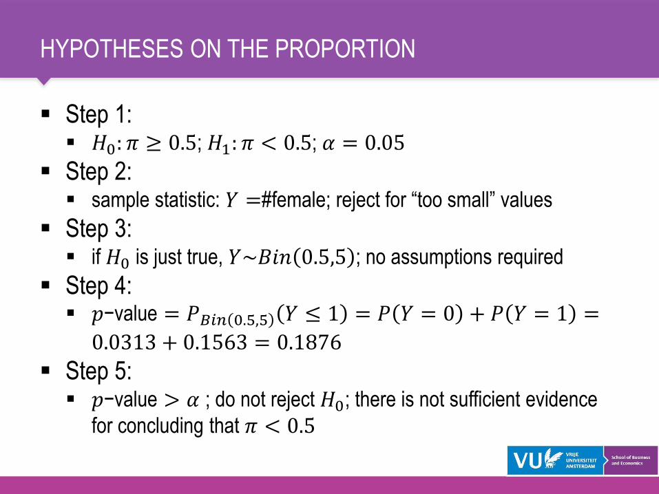
▪ Step 1:▪ 𝐻0: 𝜋 ≥ 0.5; 𝐻1: 𝜋 < 0.5; 𝛼 = 0.05

▪ Step 2:▪ sample statistic: 𝑌 =#female; reject for “too small” values

▪ Step 3:▪ if 𝐻0 is just true, 𝑌~𝐵𝑖𝑛 0.5,5 ; no assumptions required

▪ Step 4:▪ 𝑝−value = 𝑃𝐵𝑖𝑛 0.5,5 𝑌 ≤ 1 = 𝑃 𝑌 = 0 + 𝑃 𝑌 = 1 =

0.0313 + 0.1563 = 0.1876

▪ Step 5:▪ 𝑝−value > 𝛼 ; do not reject 𝐻0; there is not sufficient evidence

for concluding that 𝜋 < 0.5

HYPOTHESES ON THE PROPORTION

What if we have a large sample, say 𝑛 = 100?

▪ binomial tables and formulas don’t work

Use normal approximation

▪ if 𝑌~𝐵𝑖𝑛 𝜋, 𝑛 then 𝑍 =𝑌−𝑛𝜋

𝑛𝜋 1−𝜋~𝑁 0,1

▪ conditions: 𝑛𝜋 ≥ 5 and 𝑛 1 − 𝜋 ≥ 5: OK

Example

▪ same as before (car accidents by gender)

▪ but now based on 𝑛 = 100▪ with 𝑦 = 40 observed accidents by women

HYPOTHESES ON THE PROPORTION

▪ Step 1:▪ 𝐻0: 𝜋 ≥ 0.5; 𝐻1: 𝜋 < 0.5; 𝛼 = 0.05

▪ Step 2:▪ sample statistic: 𝑌 =#female; reject for “too small” values

▪ Step 3:

▪ if 𝐻0 is just true, 𝑍 =𝑌−𝑛𝜋

𝜎𝑌=

𝑌−𝑛𝜋

𝑛𝜋 1−𝜋~𝑁 0,1

▪ normal approximation OK (𝑛𝜋 ≥ 5 and 𝑛 1 − 𝜋 ≥ 5)

▪ Step 4:

▪ 𝑧𝑐𝑎𝑙𝑐 =40−100×0.5

100×0.5 1−0.5= −2.00 (see, however, next page!)

▪ 𝑧𝑐𝑟𝑖𝑡 = −1.645

▪ Step 5:▪ reject 𝐻0, accept 𝐻1; there is sufficient evidence for concluding that 𝜋 < 0.5

HYPOTHESES ON THE PROPORTION

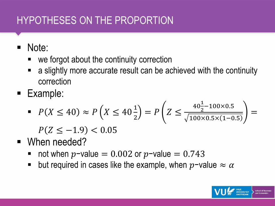
▪ Note:▪ we forgot about the continuity correction

▪ a slightly more accurate result can be achieved with the continuity

correction

▪ Example:

▪ 𝑃 𝑋 ≤ 40 ≈ 𝑃 𝑋 ≤ 401

2= 𝑃 𝑍 ≤

401

2−100×0.5

100×0.5× 1−0.5=

𝑃 𝑍 ≤ −1.9 < 0.05

▪ When needed?▪ not when 𝑝−value = 0.002 or 𝑝−value = 0.743▪ but required in cases like the example, when 𝑝−value ≈ 𝛼

HYPOTHESES ON THE PROPORTION

21 May 2015, Q1m

OLD EXAM QUESTION

Doane & Seward 5/E 11.1-11.2

Tutorial exercises week 5

confidence intervals

hypothesis tests (binomial)

hypothesis tests (normal)

FURTHER STUDY