74 December 20061527-3342/06/$20.00©2006 IEEE

© DIGITALSTOCK

The science of radio astronomy involves thedetection of radio waves from astronomicalobjects in space. Astronomical objects emitradio waves by a variety of processes,including thermal radiation from gas and

dust in the interstellar medium, synchrotron emissionfrom relativistic electrons spiraling around magneticfields, free-free emission from electrons in ionizedregions, and spectral line radiation from atomic and mol-

ecular transitions. Since the sources that radioastronomers observe are generally very distant, the inten-sity of radio waves from them is extremely low. This iscompounded by the fact that the bandwidth of spectrallines is very small. For example, a cloud of atomic hydro-gen with internal motions of 5 km/s emits only over abandwidth of 25 kHz. A source at temperature T pro-duces a maximum signal power P = kTB, where k is theBoltzmann’s constant (1.38 × 10−23 W/K-Hz) and B is

Jagadheep D. Pandian (jagadheep@astro.cornell.edu) is with Cornell University. Lynn Baker and German Cortes are with NAIC/CornellUniversity. Paul F. Goldsmith is with Cornell University/Jet Propulsion Laboratory. Avinash A. Deshpande is with Arecibo Observatory/RamanResearch Institute. Rajagopalan Ganesan and Jon Hagen are with Arecibo Observatory. Lisa Locke is with Arecibo Observatory/NRAO, Socorro.

Niklas Wadefalk is with Jet Propulsion Laboratory/Chalmers Institute of Technology. Sander Weinreb is with Jet Propulsion Laboratory.

Jagadheep D. Pandian, Lynn Baker, German Cortes, Paul F. Goldsmith, Avinash A. Deshpande,

Rajagopalan Ganesan, Jon Hagen, Lisa Locke, Niklas Wadefalk, and Sander Weinreb

December 2006 75

the bandwidth. For a relatively warm interstellar cloud at100 K, the signal power is no greater than 3.5 × 10−17 W, avery weak signal. Some signals are nonthermal and canbe stronger than this, but astronomers typically makemaps of the radio sky, which requires pointing the anten-na successively in different directions. To cover a signifi-cant area of the sky with a small antenna beam width,thousands to many millions of separate pointings andintegrations are needed. As a result, the time that can bespent analyzing the signal from any one direction is lim-ited. A very sensitive system to detect and analyze radioastronomical signals is thus extremely desirable.

All radio telescope systems have three basic compo-nents: an antenna to collect the incident radiation, areceiver to detect this radiation, and a back-end system,which analyzes the signals. The functioning of theback-end system depends on what type of signal isbeing observed—it may simply measure the totalpower in a broadband or continuum signal, or it maysplit the signal into several relatively narrow bands andmeasure the power in each, thereby producing a spec-trum of the incident radiation. The most familiar typeof radio telescope comprises a parabolic dish thatfocuses radiation into the receiver with or without theaid of a secondary reflector. Dual reflector radio anten-na systems can be of the Cassegrain or Gregorian type,similar to their counterparts at optical wavelengths.The overall sensitivity of the system is controlled pri-marily by the size and the efficiency of the antenna andthe sensitivity of the receiver.

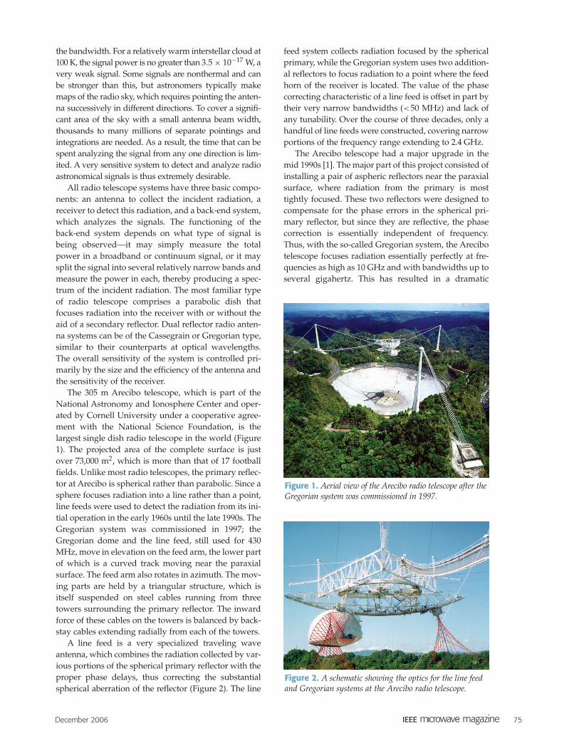
The 305 m Arecibo telescope, which is part of theNational Astronomy and Ionosphere Center and oper-ated by Cornell University under a cooperative agree-ment with the National Science Foundation, is thelargest single dish radio telescope in the world (Figure1). The projected area of the complete surface is justover 73,000 m2, which is more than that of 17 footballfields. Unlike most radio telescopes, the primary reflec-tor at Arecibo is spherical rather than parabolic. Since asphere focuses radiation into a line rather than a point,line feeds were used to detect the radiation from its ini-tial operation in the early 1960s until the late 1990s. TheGregorian system was commissioned in 1997; theGregorian dome and the line feed, still used for 430MHz, move in elevation on the feed arm, the lower partof which is a curved track moving near the paraxialsurface. The feed arm also rotates in azimuth. The mov-ing parts are held by a triangular structure, which isitself suspended on steel cables running from threetowers surrounding the primary reflector. The inwardforce of these cables on the towers is balanced by back-stay cables extending radially from each of the towers.

A line feed is a very specialized traveling waveantenna, which combines the radiation collected by var-ious portions of the spherical primary reflector with theproper phase delays, thus correcting the substantialspherical aberration of the reflector (Figure 2). The line

feed system collects radiation focused by the sphericalprimary, while the Gregorian system uses two addition-al reflectors to focus radiation to a point where the feedhorn of the receiver is located. The value of the phasecorrecting characteristic of a line feed is offset in part bytheir very narrow bandwidths (<50 MHz) and lack ofany tunability. Over the course of three decades, only ahandful of line feeds were constructed, covering narrowportions of the frequency range extending to 2.4 GHz.

The Arecibo telescope had a major upgrade in themid 1990s [1]. The major part of this project consisted ofinstalling a pair of aspheric reflectors near the paraxialsurface, where radiation from the primary is mosttightly focused. These two reflectors were designed tocompensate for the phase errors in the spherical pri-mary reflector, but since they are reflective, the phasecorrection is essentially independent of frequency.Thus, with the so-called Gregorian system, the Arecibotelescope focuses radiation essentially perfectly at fre-quencies as high as 10 GHz and with bandwidths up toseveral gigahertz. This has resulted in a dramatic

Figure 1. Aerial view of the Arecibo radio telescope after theGregorian system was commissioned in 1997.

Figure 2. A schematic showing the optics for the line feedand Gregorian systems at the Arecibo radio telescope.

76 December 2006

increase in the range of astronomical observations thatcan be carried out and also has significantly improvedthe system’s sensitivity due to better illumination ofthe primary reflector. As shown in Figure 2, the twoGregorian reflectors are enclosed by a protectivedome. The radio signals enter through the circularaperture at the bottom left of the dome and follow thepaths indicated by the red lines, reflecting from the sec-ondary then the tertiary. With the Gregorian system, theArecibo telescope focuses radiation to a point (as indi-cated in the figure) or more accurately, to a spot whereit is collected by a fairly typical feed horn, which in thiscase is oriented downward.

Thus, for the Arecibo Gregorian receivers, as foralmost all radio astronomical systems, the first compo-nent is the feed horn. The feed horn converts the incidentfree space transverse electromagnetic radiation into awaveguide transverse electric or transverse magneticmode. In this sense, the angular width of the receivingpower pattern of the feedhorn must match the angularsize of the cone of radiation coming from the antenna.Taking advantage of the reciprocity principle, we canalso think of replacing the receiver by a transmitter, andthus the feedhorn radiates a signal with an angulartransmitting power pattern, which is the same as thereceiving power pattern. This pattern of the feed horndetermines the efficiency with which the antenna oper-ates, in particular, the aperture efficiency and antennagain (relevant for point sources) and the main beam effi-ciency (relevant for extended sources). The feed hornalso needs to have a very low reflection coefficient sothat most of the signal is transmitted to the receiver. Theoutput waveguide from the feed horn typically propa-gates both polarizations of the incoming signal.

Since most signals from space are unpolarized or, ifpartially polarized, have a random polarization angle, asimple conversion of the electromagnetic signal fromspace into a guided wave in a single mode waveguidewill result in the loss of approximately half the signal. Toattain full efficiency as well as to measure the polariza-tion state of the incident signal, it is necessary to have adevice that separates the two orthogonal polarizationsbefore they are each channeled into a single mode wave-guide. This task is accomplished by the ortho-modetransducer (OMT). The OMT needs to have a return lossof 15 dB or better over the entire band of interest, in addi-tion to having a low insertion loss. To carry out goodpolarimetry, the cross polarization introduced by theOMT should be less than that induced by the feed horn.The OMT is typically the most challenging part of a dualpolarization broadband receiver design.

The outputs from the OMT are amplified using low-noise amplifiers. The low-noise amplifier and the stagefollowing it are the primary contributors to the receivernoise temperature, since noise from successive compo-nents of the receiver are suppressed by the gain of theamplifier. To achieve very low noise, the amplifier andthe OMT are typically cooled to temperatures that canbe as low as 2–15 K. This requires the receiver compo-nents to be placed in an evacuated dewar. Moreover,since most designs keep the feed horn at room temper-ature (due to its relatively large size), there needs to bea device that thermally isolates the feed horn from theOMT while maintaining continuity for the RF signal.This device is called a thermal break and typically useschoke grooves to minimize signal reflections.

The upgrade of the Arecibo telescope allowed opera-tions up to a frequency of 10 GHz. Before 2004, the tele-scope had receivers for all frequencies between 1.1 and10 GHz, except for the 6–8 GHz frequency range of C-

Figure 3. A schematic of the finline OMT used to separateincoming fields into two orthogonal polarization components.

pol A In

pol B In

Bottom Waveguide

Top Waveguide

Resistive Card

Finline

pol A Out

pol B Out

Figure 4. Measured return loss of the OMT. The bluecurve is for polarization A, which passes straight through;the red curve is for polarization B, which passes throughthe finline.

6 6.5 7 7.5 8−35

−30

−25

−20

−15

−10

−5

0

f (GHz) →

S11

(dB

) →

pol Apol B

December 2006 77

Band (4–8 GHz). The band includes the 6.668 GHz spec-tral line of methanol, which emits stimulated radiationwith very high brightness temperature (>1010 K) underconditions found around sites of massive star formation.Hitherto, all 6.7 GHz methanol maser studies have beencarried out using Australian and European telescopes.

This article reports on the 6–8 GHz receiver that wasinstalled on the telescope in early 2004. With the instal-lation of this instrument, Arecibo has continuous fre-quency coverage between 1.1 and 10 GHz. The follow-ing discusses the receiver design and presents the mea-sured performance in detail.

The Ortho-Mode TransducerWe adopted a finline design for the OMT from the workof Chattopadhyay and Carlstrom [2] (Figure 3). A finlineOMT consists of a thin metallic fin that is set inside asquare or circular waveguide. The polarization modewhich has an electric field parallel to the fin, is convert-ed from a waveguide mode into a finline mode whoseenergy is confined to the space between the fin. Thisenergy can then be brought out by curving the fin andbringing it out of the wall of the waveguide, after whichit is converted back into a waveguide mode by a gradualoutward taper. The orthogonal polarization has electricfield perpendicular to the fin and passes unperturbed ifthe fin is sufficiently thin. A resistive card suppresses anyunwanted modes at the termination of the fin.

The design of Chattopadhyay and Carlstrominvolved the removal of the finline mode through a 45◦bend, which was found to give better cross polarizationand isolation performance compared to a 90◦ bend. Wetook their prototype design for X-Band and scaled it toour band with some modifications. We replaced themultiple transitions between the finline and the normalwaveguide after the bend with a single, longer transi-tion, as a traveling wave device is likely to give a betterperformance with a longer transition. Using the samereasoning, we also lengthened the initial transition inthe finline from square waveguide to the narrow gap.

The rectangular waveguide used for 6–8 GHz isWR137, which has dimensions of 3.48 × 1.58 cm(1.372 × 0.622 in). Hence, the square waveguide inputfor the OMT has an interior dimension of 3.48 cm (1.372in). This is tapered to 0.038 cm (0.015 in) in the finlinethrough two circular arcs over a length of 27.13 cm(10.68 in). Following the 45◦ bend, the narrow gap isexpanded to the standard dimension of 1.58 cm (0.622in) over a length of 20.32 cm (8.0 in). The fin is made outof a 0.13 cm (0.05 in) thick aluminum sheet.

Figures 4–7 show the measured performance (atroom temperature) of the OMT fabricated from thedesign above. The measurements were taken with oneport being terminated by a tapered ferrite rod and theother two ports being connected to the network ana-lyzer. The return loss conformed to our design goalsave for a small portion in the band edge near 6 GHz.

Figure 7. Measured isolation between the two output portsof the OMT.

6 6.5 7 7.5 8−80

−70

−60

−50

−40

−30

−20

f (GHz) →

Isol

atio

n (d

B)

→

Figure 6. Measured cross-polarization isolation of theOMT. The blue line is for input polarization A when theoutput is measured at pol B, and the red curve is for polar-ization B input polarization when the output is measuredat pol A. The third port is terminated appropriately duringthese measurements.

6 6.5 7 7.5 8−40

−35

−30

−25

−20

−15

−10

0

f (GHz) →

Cro

ss P

ol (

dB)

→−5

Figure 5. Measured insertion loss of the OMT. The bluecurve is for polarization A, which passes straight through;the red curve is for polarization B, which passes throughthe finline.

6 6.5 7 7.5 8−2.5

−2

−1.5

−1

−0.5

0

f (GHz) →

S21

(dB

) →

pol Apol B

78 December 2006

The isolation (coupling between the two output portswhen the input is terminated) was 50 dB or better overthe entire band, and the cross polarization isolation wasbetter than 25 dB throughout. The insertion loss is pri-marily ohmic, and its contribution to the noise temper-ature would drop significantly when the device iscooled from room temperature to around 15 K.

The Feed HornThe 6–8 GHz feed horn used in the receiver is a wideflare angle corrugated horn [3]. For the present design,we chose a 78◦ flare angle that provides an edge taper

level of −15 dB at the edge of the tertiary Gregorianreflector (approximately 60◦ off axis) in the middle ofthe frequency band. In addition, we decided to havethe corrugations running parallel to the horn axis forfabrication purposes.

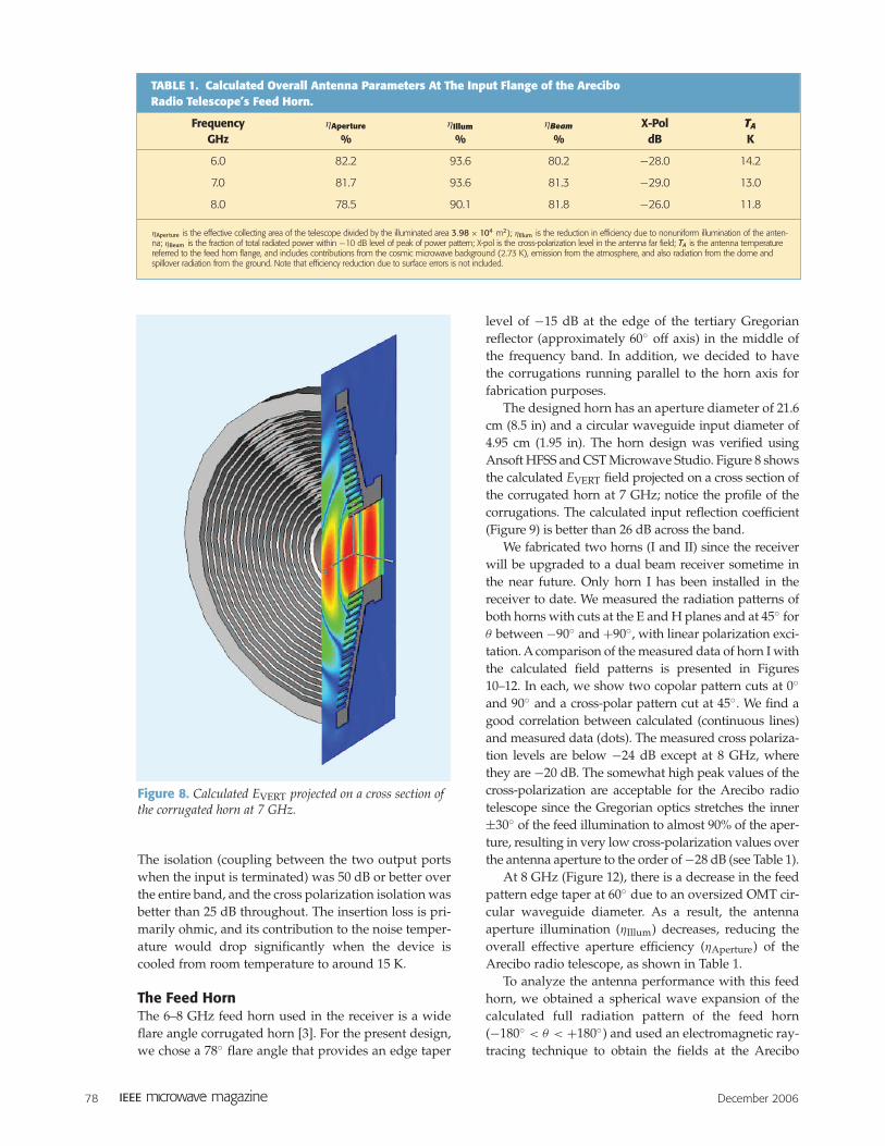
The designed horn has an aperture diameter of 21.6cm (8.5 in) and a circular waveguide input diameter of4.95 cm (1.95 in). The horn design was verified usingAnsoft HFSS and CST Microwave Studio. Figure 8 showsthe calculated EVERT field projected on a cross section ofthe corrugated horn at 7 GHz; notice the profile of thecorrugations. The calculated input reflection coefficient(Figure 9) is better than 26 dB across the band.

We fabricated two horns (I and II) since the receiverwill be upgraded to a dual beam receiver sometime inthe near future. Only horn I has been installed in thereceiver to date. We measured the radiation patterns ofboth horns with cuts at the E and H planes and at 45◦ forθ between −90◦ and +90◦, with linear polarization exci-tation. A comparison of the measured data of horn I withthe calculated field patterns is presented in Figures10–12. In each, we show two copolar pattern cuts at 0◦and 90◦ and a cross-polar pattern cut at 45◦. We find agood correlation between calculated (continuous lines)and measured data (dots). The measured cross polariza-tion levels are below −24 dB except at 8 GHz, wherethey are −20 dB. The somewhat high peak values of thecross-polarization are acceptable for the Arecibo radiotelescope since the Gregorian optics stretches the inner±30◦ of the feed illumination to almost 90% of the aper-ture, resulting in very low cross-polarization values overthe antenna aperture to the order of −28 dB (see Table 1).

At 8 GHz (Figure 12), there is a decrease in the feedpattern edge taper at 60◦ due to an oversized OMT cir-cular waveguide diameter. As a result, the antennaaperture illumination (ηIllum) decreases, reducing theoverall effective aperture efficiency (ηAperture) of theArecibo radio telescope, as shown in Table 1.

To analyze the antenna performance with this feedhorn, we obtained a spherical wave expansion of thecalculated full radiation pattern of the feed horn(−180◦ < θ < +180◦) and used an electromagnetic ray-tracing technique to obtain the fields at the Arecibo

Figure 8. Calculated EVERT projected on a cross section ofthe corrugated horn at 7 GHz.

TABLE 1. Calculated Overall Antenna Parameters At The Input Flange of the AreciboRadio Telescope’s Feed Horn.

Frequency ηAperture ηIllum ηBeam X-Pol TA

GHz % % % dB K

6.0 82.2 93.6 80.2 −28.0 14.2

7.0 81.7 93.6 81.3 −29.0 13.0

8.0 78.5 90.1 81.8 −26.0 11.8

ηAperture is the effective collecting area of the telescope divided by the illuminated area 3.98 × 104 m2); ηIllum is the reduction in efficiency due to nonuniform illumination of the anten-na; ηBeam is the fraction of total radiated power within −10 dB level of peak of power pattern; X-pol is the cross-polarization level in the antenna far field; TA is the antenna temperaturereferred to the feed horn flange, and includes contributions from the cosmic microwave background (2.73 K), emission from the atmosphere, and also radiation from the dome andspillover radiation from the ground. Note that efficiency reduction due to surface errors is not included.

December 2006 79

aperture and in the far field. From these, we calculatedthe antenna parameters from 6–8 GHz, some of whichare presented in Table 1, which includes the apertureefficiency, ηAperture (effective collecting area of the tele-scope divided by the illuminated area, which is3.98 × 104 m2), aperture illumination efficiency, ηIllum(reduction in efficiency due to nonuniform illumina-tion of the antenna), 10 dB beam efficiency, ηBeam (frac-tion of total radiated power within −10 dB of peak ofpower pattern), cross-polarization level in the antennafar field, X-Pol, and the antenna temperature, TA

(includes contributions from the 2.73 K cosmicmicrowave background radiation, emission from theatmosphere, and radiation from the dome and spilloverradiation from the ground). All these values are calcu-lated at the feed horn input flange. Reduction of effi-ciency due to surface errors is not included.

The calculated values of aperture efficiency includeblockage losses, aperture phase efficiencies, andspillover efficiencies not shown individually in thetable. Table 1 shows the decrease in aperture efficiencyat 8 GHz due to the reduced illumination efficiency.

Figure 9. Calculated horn input reflection coefficient as afunction of frequency.

0

−10

−20

−30

−40

−50

S – Parameters

6 7 8

|S11

| [dB

]

Frequency [GHZ]

Figure 10. Calculated (continuous lines) and measured(dots) copolar radiation patters cuts at 0◦ and 90◦ andcross polar at 45◦ (Horn–I at 6 GHz).

0

−10

−20

−30

−40−50 0 50

6 Ghz Pol: VERT

Rel

ativ

e P

ower

[dB

] Mean C–Pol, φ = 0° Mean C–Pol, φ = 90° Mean X–Pol, φ = 45°

θ°

Figure 11. Calculated (continuous lines) and measured(dots) copolar radiation patters cuts at 0◦, 90◦ and Cross-polar at 45◦ (Horn–I at 7 GHz).

0

−10

−20

−30

−40

7 GHz Pol: VERT

−50 0 50

Rel

ativ

e P

ower

[dB

]

θ°

Mean C–Pol, φ = 0°Mean C–Pol, φ = 90°Mean X–Pol, φ = 45°

Figure 12. Calculated (continuous lines) and measured(dots) copolar radiation patters cuts at 0◦ and 90◦ andcross-polar at 45◦ (Horn–I at 8 GHz).

0

−10

−20

−30

−40−50 0 50

8 GHz Pol: VERT

Rel

ativ

e P

ower

[dB

]

Meas C–Pol, φ = 0° Meas C–Pol, φ = 90° Meas X–Pol, φ = 45°

θ°

80 December 2006

The calculated cross-polarization values in the antennafar field are below −26 dB. The antenna noise tempera-ture values decrease as a function of frequency due tothe reduction of the size of the feed beam.

Thermal BreakThe feed horn and the dewar window are kept at roomtemperature (300 K) while the rest of the signal pathstarting with the OMT are cooled to 15 K. Hence, thereneeds to be a device that thermally isolates the 300 Kstage from the 15 K stage. This is achieved using a ther-mal break. A thermal break comprises two waveguidesthat are separated from each other by a very small gap.A choke groove device is placed at the gap so that theimpedance as seen at the wall of the waveguide is closeto zero across most of the band. The design of thischoke groove is described in the following.

The basic schematic of the choke groove is shownin Figure 13. The parameters to be determined are thelocation of the coaxial waveguide, Rc, and the heightof the groove (or length of the coaxial waveguide),which should be one-quarter of the guide wavelengthin the coaxial waveguide, λg. This involves a knowl-edge of the electromagnetic wave propagation both

radially outward along the gap and axially along thecoaxial waveguide.

Figure 14 shows a schematic of the coaxial wave-guide, which is treated as a rolled up thin rectangularwaveguide. If the height h of the waveguide is smallcompared to its radius, we can analyze it as if it werenot rolled up at all, except for the boundary conditionthat the field is periodic with period C, whereC = 2πRc, is the circumference of the waveguide. Thedirection of the E field will be in the y direction. FromMaxwell’s equations, the wave propagation equationin the waveguide is

∂2E∂x2 −

(k2

z − k20

)E = 0, (1)

where k0 = 2π/λ0 and λ0 is the free-space wavelength.Now, the boundary condition requires that the depen-dence of E on x be of the form cos(2πnx/C). Since thewaveguide mode under consideration is TE11, we haven = 1. Hence, we have

∂2E∂x2 +

(2π

C

)2E = 0. (2)

From the two equations above, we get

kz =√

k20 −

(2π

C

)2. (3)

The guide wavelength λg is given by 2π/kz, whichbecomes

λg = λ0√1 −

(λ0

2πRc

)2. (4)

This gives the height of the choke groove, once Rc isdetermined (as described below).

In the radial waveguide (the section of the gapbetween the main circular waveguide and the coaxialwaveguide), the electric field is a function of only r andθ , where (r, θ) refer to polar coordinates. The field can-not be a function of z as its divergence would then notbe zero. From Maxwell’s equations, we have

Figure 13. Schematic of a thermal break with a chokegroove. (a) A cross section of the device, which comprises atop piece and a bottom piece that are thermally isolatedthrough stand-offs made from a material like G10 fiber-glass. (b) The bottom view of the top piece. The innerradius of the circular waveguide is Rg and that of thechoke groove is Rc.

Rgλg/4

Rc

r

Bottom View of Top PieceCross-Section of Thermal Break

CoaxialWaveguide

Figure 14. A coaxial waveguide can be treated as a rolled up thin rectangular waveguide.

yz

h

x

∇ × ∇ × E − k20E = 0. (5)

Taking the z component of above gives

(∇ × ∇ × E)z =1r

∂

∂ r

(r∂Ez

∂ r

)− 1

r∂

∂θ

(1r

∂Ez

∂θ

)

=k20Ez. (6)

The angular dependence of Ez must again be propor-tional to cos(nθ), where for the same reason as before,n = 1. Thus, the above equation becomes

∂2Ez

∂ r2 + 1r

∂Ez

∂ r+

(k2

0 − 1r2 Ez

)= 0. (7)

The solutions to this equation are the Bessel functionsJ1(k0r) and Y1(k0r), and the radial part of Ez is a linearcombination of the two:

Ez(r) = J1(k0r) + a Y1(k0r). (8)

The location of the groove (coaxial waveguide) cannow be determined as follows. The purpose of thechoke groove is to make the gap look like the wall of anormal waveguide, and hence the E field in the gap iszero at r = Rg. Hence, the first task is to determine thelinear combination of Bessel functions (the parametera) that will give rise to a zero at r = Rg. Then, the loca-tion of the groove is given by the value of r that maxi-mizes or minimizes this linear combination. Once Rc isdetermined, λg can be calculated, which gives theheight of the groove.

In our case, the circular waveguide had a radiusRg = 2.48 cm (0.975 in). Doing the calculationdescribed above, we determined Rc to be 3.51 cm (1.38in). The guide wavelength in the coaxial waveguide, λg,turned out to be 4.42 cm (1.74 in), and hence the grooveheight was set to 1.10 cm (0.435 in). The gap in thewaveguide is set to be as small as practical for betterperformance and in our case, turned out to be 0.018 cm(0.007 in). We had two thermal breaks in the dewar, onefor isolating the 70 K stage from the 300 K stage andanother for isolating the 15 K stage from the 70 K stage.This was done so as to reduce the heat load on the sec-ond stage of the refrigerator (which nominally coolsdown to 15 K). Indeed, the use of two thermal breakslowered the heat load to allow the second stage to cooldown to around 10.5 K during actual operation, whichin turn lowered ohmic contribution to the receivernoise temperature.

Low-Noise AmplifiersThe low-noise amplifiers used in the receiver utilize amonolithic-microwave integrated circuit (MMIC) thatwas designed at Caltech [4] and fabricated in theNorthrop Grumman semiconductor foundry. The mod-

ule is shown in Figure 15 with a closeup of the MMICin Figure 16. The MMIC is the type WBA13, which uti-lizes three indium-phosphide high-electron-mobilitytransistors (HEMTs) with 0.1 µm gate length. Theamplifiers have extremely low noise (<4 K) over a verywide bandwidth (4–12 GHz) when cooled to 12 K, asshown in Figure 17. Over 50 of these amplifiers withvery repeatable performance have been built atCaltech. At 300 K, the noise temperature of the amplifi-er is approximately 50 K (0.7 dB noise figure).

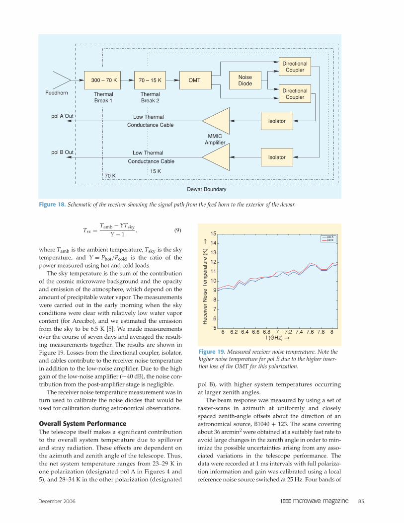
Remainder of the Signal PathThe overall signal path in the receiver is shown inFigure 18. The low-noise amplifier is preceded by anisolator and a directional coupler. The isolator wasfrom Passive Microwave Technology and had specifi-cations of 20 dB isolation with an input and outputvoltage standing wave ratio (VSWR) of 1.24 and aninsertion loss of less than 0.38 dB (which was verifiedthrough actual measurements). The directional cou-plers are used for injecting power from a noise diodeand are used for calibration purposes during

December 2006 81

Figure 15. LNA module with covers removed. The moduleis comprised of input, output, dc bias circuit boards, and anInP MMIC three-stage amplifier, shown in Figure 16.

Figure 16. WBA13 MMIC used in the amplifier. The chipsize is 2 mm × 0.73 mm. The bond wires are for input, out-put, gate, and drain voltage. In addition to the three tran-sistors, the chip contains thin-film resistors and capacitorsand spiral inductors. Over 1,000 amplifiers can be pro-duced on one 3-in wafer.

82 December 2006

astronomical observations. The couplers were fromMAC Tech, and had return loss of less than 25 dB,insertion loss of less than 0.15 dB, coupling of30 ± 1.25 dB, and a directivity better than 30 dB,which were well within specifications.

The output from the low-noise amplifier is thentaken out of the dewar and converted to a center fre-quency of 1.5 GHz. This is in turn transmitted over anoptical fiber link to the signal processing area in abuilding adjacent to the telescope. There, a digitalautocorrelation spectrometer produces spectra. Longstainless steel cables with beryllium copper inner con-

ductors were used between the refrigerator stages tominimize conductive heat loads on the refrigerator.

Receiver Noise TemperatureWe evaluated the overall noise temperature of thereceiver using the Y-factor method. The receiver wasmounted such that the feed horn was looking at thesky, which served as the cold load. Then, a piece ofEccosorb absorbing material was placed in front of thehorn to serve as the hot load. By measuring the receiv-er power with the two loads, the noise temperature ofthe receiver, Trx, can be evaluated by

Figure 17. Measured gain and noise temperature at 12 K at four different bias settings for a typical LNA of the type used inthe receiver. The highest bias power of 24 mW results in 41 dB gain and 3.5 K noise averaged from 4–12 GHz, while a lowerbias power of 3.9 mW still results in 33 dB gain and 4.8 K average noise.

Gain [dB] bp1

Gain [dB] bp2

Gain [dB] bp3

Gain [dB] bp4

Noise [K] bp1

Noise [K] bp2

Noise [K] bp3

Noise [K] bp4

4-12GHz LNA#06D at 12KCIT1 4254-065 R2C 1M1

45

40

35

30

25

20

15

10

5

0

45

40

35

30

25

20

15

10

5

02 4 6 8 10 12 14 16

Noise [K

]Gai

n [d

B]

Bp1:Vd=1.20V

Id=20.00mAVg1=Vg2=2.84V

Tavg=3.49K

Bp2:Vd=1.00V

Id=15.00mAVg1=Vg2=2.80V

Tavg=3.63K

Bp3:Vd=0.8V

Id=11.5mAVg1=Vg2=2.80V

Tavg=3.89K

Bp4:Vd=0.50VId=7.8mA

Vg1=Vg2=2.80VTavg=4.80K

Frequency [GHz]

December 2006 83

Trx = Tamb − YTsky

Y − 1, (9)

where Tamb is the ambient temperature, Tsky is the skytemperature, and Y = Phot/Pcold is the ratio of thepower measured using hot and cold loads.

The sky temperature is the sum of the contributionof the cosmic microwave background and the opacityand emission of the atmosphere, which depend on theamount of precipitable water vapor. The measurementswere carried out in the early morning when the skyconditions were clear with relatively low water vaporcontent (for Arecibo), and we estimated the emissionfrom the sky to be 6.5 K [5]. We made measurementsover the course of seven days and averaged the result-ing measurements together. The results are shown inFigure 19. Losses from the directional coupler, isolator,and cables contribute to the receiver noise temperaturein addition to the low-noise amplifier. Due to the highgain of the low-noise amplifier (∼40 dB), the noise con-tribution from the post-amplifier stage is negligible.

The receiver noise temperature measurement was inturn used to calibrate the noise diodes that would beused for calibration during astronomical observations.

Overall System PerformanceThe telescope itself makes a significant contributionto the overall system temperature due to spilloverand stray radiation. These effects are dependent onthe azimuth and zenith angle of the telescope. Thus,the net system temperature ranges from 23–29 K inone polarization (designated pol A in Figures 4 and5), and 28–34 K in the other polarization (designated

pol B), with higher system temperatures occurringat larger zenith angles.

The beam response was measured by using a set ofraster-scans in azimuth at uniformly and closelyspaced zenith-angle offsets about the direction of anastronomical source, B1040 + 123. The scans coveringabout 36 arcmin2 were obtained at a suitably fast rate toavoid large changes in the zenith angle in order to min-imize the possible uncertainties arising from any asso-ciated variations in the telescope performance. Thedata were recorded at 1 ms intervals with full polariza-tion information and gain was calibrated using a localreference noise source switched at 25 Hz. Four bands of

Figure 19. Measured receiver noise temperature. Note thehigher noise temperature for pol B due to the higher inser-tion loss of the OMT for this polarization.

6 6.2 6.4 6.6 6.8 7 7.2 7.4 7.6 7.8 85

6

7

8

9

10

11

12

13

14

15

f (GHz) →

Rec

eive

r N

oise

Tem

pera

ture

(K

) →

pol A pol B

Figure 18. Schematic of the receiver showing the signal path from the feed horn to the exterior of the dewar.

NoiseDiode

DirectionalCoupler

DirectionalCoupler

Isolator

Isolator

MMICAmplifier

OMT70 – 15 K

ThermalBreak 2

300 – 70 K

ThermalBreak 1

Feedhorn

Low Thermal

Conductance Cable

Low Thermal

Conductance Cable

15 K70 K

Dewar Boundary

pol B Out

pol A Out

84 December 2006

100 MHz width each around 6.6 GHz were observedwith 128 spectral channels per band, and the spectraldata were combined later to obtain a band-averagedresponse. Suitable regridding and interpolation wereperformed to obtain a beam map with fine and uniformsampling in the azimuth and the zenith-angle offsets.The estimated response in Stokes I is shown in Figure20. The elliptical beam pattern is a result of the finalillumination aperture of diameter 213 × 237 m [6]. Thecoma side-lobe is apparent around the main responsewhose angular widths in the two directions are consis-

tent with the expectation. Figure 21 displays twoorthogonal cuts sampled through and normalized tothe peak response. The coma response is seen to be, onaverage, below −12 dB of the main beam peak.

At present, the feed horn, isolators, directional cou-plers, and low-noise amplifiers for the second beam arenot installed. Consequently, the receiver is working as anormal single-beam instrument at present. It is expectedto be upgraded to a full dual-beam receiver by early 2007.

ConclusionsThe combination of the traveling wave OMT device andthe ultra-low-noise MMIC amplifiers has allowed us todevelop a broadband 6–8 GHz receiver with a noisetemperature of around 10 K. The combination of receiv-er noise and the additional noise contributions by thetelescope optics gives an overall receiver temperature ofaround 28 K and 34 K in the two polarizations. The largecollecting area of the telescope gives rise to a systemequivalent flux density of around 4.5 Jy at 7 GHz.

References[1] P.F. Goldsmith, “The second arecibo upgrade,” IEEE Potentials,

vol. 15, pp. 38–43, Aug.–Sept. 1996.[2] G. Chattopadhyay and J.E. Carlstrom, “Finline ortho-mode trans-

ducer for millimeter waves,” IEEE Microwave Guided Wave Lett.,vol. 9, pp. 339–341, Sept. 1999.

[3] P.J.B. Clarricoats and A.D. Olver, Corrugated Horns for MicrowaveAntennas (IEEE Electromagnetic Waves Series 18). Stevenage, UK:Peregrinus, 1984.

[4] N. Wadefalk and S. Weinreb, “Very low noise amplifiers for verylarge arrays,” in Proc. Workshop WFF, IEEE IMS2005 Symp., LongBeach, CA, June 2005 [CD-Rom].

[5] P.F. Goldsmith, “Calculation of atmospheric emission measuredby Gregorian feed horns,” NAIC Internal Memo, Sept. 2001.

[6] P.S. Kildal, L.A. Baker, and T. Hagfors, “The arecibo upgrading:Electrical design and expected performance of the dual-reflectorfeed system,’’ Proc. IEEE, vol. 82, pp. 714–724, May 1994.

Figure 21. The beam profiles in azimuth and zenith angle respectively, sampled from the beam-map (shown in Figure 20) ascuts through its peak, are shown in dB scale with respect to the peak response.

−3 −2 −1 0 1 2 3

0

−10

−20

−30

0

−10

−20

−30

AZ Offset (arcmin)

−3 −2 −1 0 1 2 3ZA Offset (arcmin)

Gai

n R

atio

(dB

)G

ain

Rat

io (

dB)

Figure 20. Normalized beam response mapped as a functionof offsets in azimuth and zenith-angle and estimated usingfull polarization measurements from a set of raster-scans on acontinuum source B1040 + 123. The estimates shown herecorrespond to the response in the Stokes I parameter.

ZA

Offs

et (

arcm

in)

−20

2

0 0.5 1

AZ Offset (arcmin)−2 0 2

0

0.5

1 00.

51