Tibbs, A., Daly, I., Roberts, N., & Bull, D. (2018). Denoising imagingpolarimetry by adapted BM3D method. Journal of the Optical Society ofAmerica A, 35(4), 690-701. https://doi.org/10.1364/JOSAA.35.000690

Publisher's PDF, also known as Version of record

License (if available):CC BY

Link to published version (if available):10.1364/JOSAA.35.000690

Link to publication record in Explore Bristol ResearchPDF-document

University of Bristol - Explore Bristol ResearchGeneral rights

This document is made available in accordance with publisher policies. Please cite only the publishedversion using the reference above. Full terms of use are available:http://www.bristol.ac.uk/pure/about/ebr-terms

Denoising imaging polarimetry by adaptedBM3D methodALEXANDER B. TIBBS,1,2,* ILSE M. DALY,2 NICHOLAS W. ROBERTS,2 AND DAVID R. BULL1

1Department of Electrical and Electronic Engineering, University of Bristol, Bristol BS8 1UB, UK2School of Biological Sciences, University of Bristol, Bristol BS8 1TQ, UK*Corresponding author: alex.tibbs@bristol.ac.uk

Received 31 October 2017; revised 26 February 2018; accepted 26 February 2018; posted 27 February 2018 (Doc. ID 312417);published 30 March 2018

In addition to the visual information contained in intensity and color, imaging polarimetry allows visual infor-mation to be extracted from the polarization of light. However, a major challenge of imaging polarimetry is imagedegradation due to noise. This paper investigates the mitigation of noise through denoising algorithms and com-pares existing denoising algorithms with a new method, based on BM3D (Block Matching 3D). This algorithm,Polarization-BM3D (PBM3D), gives visual quality superior to the state of the art across all images andnoise standard deviations tested. We show that denoising polarization images using PBM3D allows the degreeof polarization to be more accurately calculated by comparing it with spectral polarimetry measurements.

Published by The Optical Society under the terms of the Creative Commons Attribution 4.0 License. Further distribution of this work

must maintain attribution to the author(s) and the published article’s title, journal citation, and DOI.

OCIS codes: (100.3020) Image reconstruction-restoration; (120.5410) Polarimetry.

https://doi.org/10.1364/JOSAA.35.000690

1. INTRODUCTION

The polarization of light describes how light waves propagatethrough space [1]. Although different forms of polarization canoccur, such as circular polarization, in this paper we focus onlyon linear polarization, the form that is abundant in nature.Light is said to be completely linearly polarized (or polarizedfor the purposes of this paper) when all waves travelling alongthe same path through space are oscillating within the sameplane. If, however, there is no correlation between the orienta-tion of the waves, the light is described as unpolarized.Polarized and unpolarized light are the limiting cases of partiallypolarized light, which can be considered to be a mixture ofpolarized and unpolarized light.

The polarization of light can be altered by the processes ofscattering and reflection. As a form of visual information, itprovides a fitness benefit such that many animals [2,3] usepolarization sensitivity for a variety of task-specific behaviorssuch as navigation [4], communication [5], and contrastenhancement [6]. Inspired by nature, many devices, knownas imaging polarimeters or polarization cameras, are now avail-able that capture images containing information about thepolarization of light [7,8]. These have been used in a growingnumber of applications [9], including mine detection [10],surveillance [11], shape retrieval [12], and robot vision [13]as well as research in sensory biology [8,14].

A major challenge facing imaging polarimetry, addressed inthis paper, is noise. State-of-the art imaging polarimeters sufferfrom low signal-to-noise ratios (SNR), and it will be shown thatconventional image denoising algorithms are not well suited topolarization imagery.

While a great deal of previous work has been done ondenoising, very little has specifically been tailored to imagingpolarimetry. Zhao et al. [15] approached denoising imagingpolarimetry by computing Stokes components from a noisycamera using spatially adaptive wavelet image fusion, whereasFaisan et al.’s [16] method is based on a modified version of thenonlocal means (NLM) algorithm [17].

This paper compares the effectiveness of conventionaldenoising algorithms in the context of imaging polarimetry.A novel method termed Polarization-BM3D (PBM3D),adapted from an existing denoising algorithm, BM3D(Block Matching 3D) [18], is then introduced and will beshown to be superior to the state of the art.

2. IMAGING POLARIMETRY

A. Representing Light Polarization

A polarizer is an optical filter that only transmits light of a givenlinear polarization. The angle between the transmitted light andthe horizontal is known as the polarizer orientation. Let I

690 Vol. 35, No. 4 / April 2018 / Journal of the Optical Society of America A Research Article

1084-7529/18/040690-12 Journal © 2018 Optical Society of America

represent the total light intensity and I i represent the intensityof light, which is transmitted through a polarizer orientated at idegrees to the horizontal. The standard way of representing thelinear polarization is by using Stokes parameters �S0; S1; S2�[19], which are defined as follows:

S0 � I ; (1)

S1 � I 0 − I 90; (2)

S2 � I 45 − I 135: (3)

Note that I � I 0 � I 90 � I 45 � I 135, so the above can berewritten, using I 0, I 45, and I 90, as

S0 � I0 � I 90; (4)

S1 � I 0 − I 90; (5)

S2 � −I 0 � 2I45 − I 90: (6)

The degree of (linear) polarization (DoP) and the angle ofpolarization (AoP) are defined as

DoP �ffiffiffiffiffiffiffiffiffiffiffiffiffiffiffiffiS21 � S22

pS0

; (7)

AoP � 1

2arctan

�S2S1

�: (8)

The DoP represents the proportion of light that is polarized,rather than being unpolarized, i.e., DoP � 1 means that thelight is fully polarized, DoP � 0 means unpolarized. The AoPrepresents the average orientation of the oscillation of multiplewaves of light, expressed as an angle from the horizontal.

B. Imaging Polarimeters

Imaging polarimeters are devices that, in addition to measuringthe intensity of light at each pixel in an array, also measure thepolarization of light at each pixel location. There are manydesigns of a passive imaging polarimeter (here, we are not con-cerned with active imaging polarimeters), summarized in [20].The common feature they share is in measuring the intensityof light, which passes through polarizers of multiple orienta-tions, �I i1 ; I i2 ;…; I in�, possibly with additional measurementsof circular polarization, at each pixel in an array. The measure-ments for multiple orientations are taken either simultaneouslyor of a completely static scene. The Stokes parameters arethen derived at each pixel. For the rest of this paper, we willconsider a polarimeter that measures I 0, I 45, and I90, whichis a common arrangement [7,8]. Generalizations to imagingpolarimeters, which measure intensities at different angles,are straightforward.

As this paper addresses polarization measurements across anarray, the symbols I0, I 45, I 90, S0, S1, S2, DoP, and AoP willhenceforth refer to the array of values, rather than a single mea-surement. I 0, I 45, and I 90 are known as the camera compo-nents and S0, S1, and S2 as the Stokes components.

C. Noise

Noise affects most imaging systems and is especially challengingin polarimetry due to the complex sensor configuration in-volved with measuring the polarization. Each type of imagingpolarimeter (see [20] for a description of the different types)

either is affected by noise to a greater extent than are conven-tional cameras or suffers from other degradations that limit itsuse to specific applications. “Division of focal plane” polarim-eters, which use micro-optical arrays of polarization elements,suffer from imperfect fabrication and crosstalk between polari-zation elements. “Division of amplitude” polarimeters, whichsplit the incident light into multiple optical paths, suffer fromlow SNR due to the splitting of the light. “Division of aperture”polarimeters, which use separate apertures for separate polari-zation components, suffer from distortions due to parallax (ex-cept in the case where a scene has no depth). “Division of time”polarimeters require static, or slowly evolving, scenes, and arethus incapable of recording video of scenes with rapid move-ment and so, for many applications, cannot be used. Also, inpolarimetry, where DoP and AoP are often the quantities ofinterest, they are nonlinear functions of the camera andStokes components, which in this case have the effect of am-plifying the noise degradation.

To highlight the degradation of a DoP image due to noise,consider Fig. 1. The top row shows the three camera compo-nents of an unpolarized scene (i.e., all three components areidentical, and DoP � 0 everywhere). The original images withnoise added are shown in the bottom row. Although there is onlya small noticeable difference between the original and noisy cam-era components, the difference between the original and noisyDoP images is severe. This indicates a large error, with 25% ofpixels exhibiting an error greater than 10%. The error is greaterwhen the intensity of the camera components is smaller. To seewhy this is the case, consider a noisy Stokes image �S0; S1; S2�,where the measured values are normally distributed around thetrue Stokes parameters �T 0; T 1; T 2�. Let the true DoP be givenby δ0 � �T 2

1 � T 22�1∕2∕T 0. The naive way to compute δ0 is to

apply the DoP formula to the measured Stokes parametersδ � �S21 � S22�1∕2∕S0. But E�δ� ≠ δ0 (where E is expectedvalue), meaning that this is a biased estimator; thus, the calcu-latedDoP does not average to the correct result. This can be seenby the fact that, if the trueDoP, δ0, is zero, andT 0 > 0, then anyerror in S1 and S2 results in δ > 0. Denoising algorithms,including the one proposed in this paper, PBM3D, are thusessential for mitigating such degradations due to noise.

This paper considers only uniformly distributed indepen-dent Gaussian noise. This noise model is only a good fit in thecase of detector-limited noise but serves as an approximation of

I0

orig

inal

nois

y

I45

I90 DOP

Fig. 1. Simulation of an unpolarized scene with and without noise(σ � 0.02). Black represents a value of 0, white of 1. The error is largefor the noisy DoP image.

Research Article Vol. 35, No. 4 / April 2018 / Journal of the Optical Society of America A 691

the shot-noise process and has precedence in the literature[15,16]. A noise model in which the Gaussian parametersare allowed to vary between pixels depending on the intensitywould have greater general applicability to polarimetry, butBM3D, on which our algorithm PBM3D is based, assumesuniformly distributed noise. In Section D, PBM3D is appliedto real polarimetry and is shown to be effective, thereby justify-ing our choice of noise model. Throughout this paper, a noisycamera component, I i, is described as follows. LetΩ denote theimage domain. For all x ∈ Ω and i ∈ f0; 45; 90g:I i�x� �I 0i�x� � n�x� where the noise, n�x�, is a normally distributedzero-mean random variable with standard deviation σ, and I i 0 isthe true camera component.

3. STATE OF THE ART

There are various methods for mitigating noise degradation inimaging polarimetry. For example, polarizer orientations can bechosen optimally for noise reduction [21,22]; however, this isnot always possible due to constraints on the imaging system.Further reductions in noise can also be made through theuse of denoising algorithms, which attempt to estimate theoriginal image.

While vast literature exists on denoising algorithms ingeneral, little is specifically targeted at denoising imaging polar-imetry. Zhao et al. [15] approached denoising imaging polar-imetry by computing Stokes components from a noisy camerausing a spatially adaptive wavelet image fusion, based on [23].A benefit of this algorithm is that the noisy camera componentsneed not be registered prior to denoising. The algorithm ofFaisan et al. [16] is based on a modified version of Buades et al.’snonlocal means (NLM) algorithm [17]. The NLM algorithm ismodified by reducing the contribution of outlier patches in theweighted average and by taking into account the constraintsarising from the Stokes components having to be mutuallycompatible. A disadvantage of this method is that it takes a longtime to denoise a single image (550s for a 256 × 256 image,which takes approximately 1 s using our method, PBM3D.Both on an Intel Core i7, running at 3 GHz).

In this paper, our PBM3D algorithm will be compared withthe above two algorithms. Faisan et al. [16] compared theirdenoising algorithm with earlier methods [24–26] and demon-strated that their NLM-based algorithm gives superior denois-ing performance. For this reason, comparison with thesealgorithms is not considered.

4. METHOD

Our approach to denoising polarization images is to adaptDabov’s BM3D algorithm [18] for use with imaging polarim-etry, a novel method that we call PBM3D.

BM3D was chosen primarily for its robustness and effective-ness. Sadreazami et al. [27] recently compared the performanceof a large number of state-of-the-art denoising algorithms, usingthree test images and four values of σ, the noise standarddeviation. The authors showed that no one denoising algorithmof those tested always gave the greatest denoised peak signal-to-noise ratio (PSNR). However, BM3D was always able to givedenoised PSNR values close to the best performing algorithmand, in more than half the cases, was in the top two. Another

appealing aspect of BM3D is that extensions have been pub-lished for color images (CBM3D) [28], multispectral images(MSPCA-BM3D) [29], volumetric data (BM4D) [30], andvideo (VBM4D) [31]. This extensibility shows the versatility ofthe core algorithm. Sadreazami et al. found that CBM3D wasthe best-performing algorithm for color images with highnoise levels.

A. BM3D

BM3D consists of two steps. In Step 1, a basic estimate of thedenoised image is produced; Step 2 then refines the estimateproduced in Step 1 to give the final estimate. Steps 1 and 2consist of the same basic substeps, as shown in Algorithm 1.

Algorithm 1: BM3D, single step

1: for each block (rectangular neighbourhood of pixels) in noisyimage do

2: find similar blocks across the image ▹ for Step 1 this is doneusing the noisy image; for Step 2 the basic estimate

3: stack similar blocks to form 3D group4: apply 3D transform to obtain sparse representation5: apply filter to denoise ▹ for Step 1 the filtering is done using a

hard thresholding operation; for Step 2 a Wiener filter is used6: invert transform7: for each pixel do8: estimate single denoised value from values of multiple

overlapping blocks9: return denoised image

BM3D is described more fully in [18], and thorough analy-sis is provided in [32].

B. CBM3D

CBM3D adapts BM3D for color images [28]. Figure 2 outlinesthe algorithm, which works by applying BM3D to the threechannels of the image in the YUV color space, also in twosteps, but computing the groups only using the Y channel.Details of CMB3D are as shown in Algorithm 2.

Algorithm 2: CBM3D, single step

1: input noisy color image2: apply color-space transform �Y ;U ; V � ← T �R; G; B� ▹ YUV

represents a chosen luminance-chrominance color space3: for each block in channel Y image do4: find similar blocks across the image ▹ for Step 1 this is done

using the noisy image; for Step 2 the basic estimate5: stack similar blocks to form 3D group6: for channels U; V do7: stack blocks to form 3D groups using the same groups as

formed in Line 58: for each channel Y ;U ; V do9: for each group do10: apply 3D transform to obtain sparse representation11: apply filter to denoise ▹ for Step 1 the filtering is done

using a hard thresholding operation; for Step 2 a Wienerfilter is used

12: invert transform13: for every pixel do14: estimate single denoised value from values of multiple

overlapping blocks15: Apply inverse color-space transform �R;G; B� ← T −1�Y ;U ; V �16: return denoised image

692 Vol. 35, No. 4 / April 2018 / Journal of the Optical Society of America A Research Article

Dabov et al. [28] provide the following reason for whyCBM3D performs better than applying BM3D separately tothree color channels:

• The SNR of the intensity channel Y is greater than thechrominance channels.

• Most of the valuable information, such as edges, shades,objects and texture, are contained in Y .

• The information in U and V tends to be low-frequency.• Isoluminant regions, with U and V varying are rare.

If BM3D is performed separately on color channels, U andV , the grouping suffers [28] due to the lower SNR, and thedenoising performance is worse, as it is sensitive to thegrouping.

C. PBM3D

In order to optimize BM3D for polarization images, wepropose taking CBM3D and replacing the RGB to YUVtransformation with a transformation from the camera compo-nent image �I 0; I 45; I90� image to a chosen polarization space,denoted generally as �P0; P1; P2�. This is shown inAlgorithm 3.

Algorithm 3: PBM3D, single step

1: input noisy polarization image2: apply polarization transform �P0; P1; P2� ← T �I 0; I 45; I 90� ▹

�P0; P1; P2� represents a chosen luminance-polarization colorspace

3: for each block in channel P0 image do4: find similar blocks across the image ▹ for Step 1 this is done

using the noisy image; for Step 2 the basic estimate5: stack similar blocks to form 3D group6: for channels P1; P2 do7: stack blocks to form 3D groups using the same groups as

formed in Line 58: for each channel �P0; P1; P2� do9: for each group do10: apply 3D transform to obtain sparse representation11: apply filter to denoise ▹ for Step 1 the filtering is done

using a hard thresholding operation; for Step 2 a Wiener filter isused

12: invert transform13: for every pixel do14: estimate single denoised value from values of multiple

overlapping blocks15: apply inverse color-space transform

�I0; I 45; I 90� ← T −1�P0; P1; P2�16: return denoised image

The choice of T has a large effect on denoising performance.Which matrix is optimal is dependent on the image statisticsand the noise level, which are both dependent on the applica-tion. A possible choice for the polarization transform is to useStokes parameters [Eqs. (4)–(6)], which is shown in Fig. 2. Thetransform to Stokes parameters (Stokes transform) results in thefirst channel, P0 � S0 being intensity, which uses argumentssimilar to those used in Section 5, is likely to contain mostof the valuable information. For this reason, the Stokes trans-form was used as a starting point in finding the optimal denois-ing matrix in Section 5.

Here, we describe an algorithm estimate of the optimalmatrix, T opt, given a set of noise-free model images, D, anda given noise standard deviation, σ.

Let Ii ∈ D be a noise-free camera component image (e.g.,I � �I0; I45; I90�), Ii 0 be Ii with Gaussian noise of standarddeviation σ added, D 0 be the set of images Ii

0and PBM3DT

represent the operation of applying PBM3D with transforma-tion matrix T . Define T opt as follows:

T opt � arg minT

XiMSE�Ii ; PBM3DT �Ii 0 ��; (9)

where MSE is the mean square error. Note that T is normalizedsuch that, for each row, � a b c �, jaj � jbj � jcj � 1.

Due to the large number of degrees of freedom of T and thefact that the matrix elements can take any value in the range�−1; 1�, it is not possible to perform an exhaustive search.Instead, a pattern search method can be used and is describedin Algorithm 4. Note that the intervals δ and 10δ are both usedto avoid converging to nonglobal minima. Results from themethod are shown in Section 5.

Algorithm 4: Pattern search method

1: choose a starting matrix T 0 and small interval δ2: i ← 03: loop4: find all perturbations of T i by δ, which preserve the

normalization condition ▹ for each row � a b c �,jaj � jbj � jcj � 1

5: find all perturbations of T i by 10δ, which preserve thenormalization condition

6: for every perturbation, P, of T i do7: for every image, I 0 ∈ D 0 do8: denoise I 0 using P9: MP ←

PiMSE�I 0; PBM3DP�I 0��

10: T i�1 ← arg minPMP11: if T i�1 � T i then return T opt ← T i12: i ← i � 1

5. EXPERIMENTS

A. Data Sets

In order to demonstrate the effectiveness of denoising algo-rithms, they must be evaluated using representative noisy testimagery. The test imagery used in these experiments comprisesnoise-free polarization images, with simulated noise. As noise-free polarization images cannot be produced using a noisy im-aging polarimeter, we instead use a digital single-lens reflex(DSLR) camera with a rotatable polarizer in front of the lens.This approach to producing imaging polarimetry is one of theearliest [33] and has been used by various authors, e.g., [6,34].

For this approach to work, the camera sensor must have alinear response with respect to intensity, that is Imeasured �kI actual, where Imeaured and I actual are the measured and actuallight intensities, and k is an arbitrary constant. The linearity canbe verified using a fixed light source and a second rotatingpolarizer. As one polarizer is kept stationary, and the other isrotated, the intensity values measured at each pixel will producea cosine squared curve if the sensor is linear, according to

Research Article Vol. 35, No. 4 / April 2018 / Journal of the Optical Society of America A 693

Malus’ law [19]. The DSLR used to generate the images in thispaper was a Nikon D70, whose sensors have a linear response.

The images are generated as follows:

1: All camera settings are set to manual for consistencybetween shots.

2: To prevent inaccuracies due to compression, the camerais set to take images in raw format.

3: The camera is placed on a tripod or otherwise such thatit is stationary.

4: The polarizer is orientated to be parallel to the horizon-tal and an image is taken.

5: The polarizer is rotated so that it is at 45 deg to thehorizontal and a second image is taken.

6: The polarizer is rotated so that it is orientated verticallyand the final image is taken.

Given the superior SNR of modern DSLR cameras, thisprovides low noise polarization images. For arbitrarily low noiselevels, multiple photos for a given polarizer angle are taken,

registered, and averaged. The main drawback of this methodis that the light conditions and image subjects must be station-ary; this method therefore cannot be used for many applica-tions but still allows noise-free polarization images to be takenand so is invaluable for testing denoising algorithms.

B. Optimal Denoising Matrix

The optimal matrix for a given application is dependent on theimage statistics and the noise level. In order to test the matrixoptimization algorithms given in Section 4, and, with no par-ticular application in mind, we produced a set of 10 polariza-tion images, using the method above, of various outdoorscenes. We added noise of several values of σ, the noise standarddeviation (see Tables 1 and 2). The optimal matrices given inthis section are therefore only optimal for this particular imageset. However, they provide a useful starting point and are likelyto be close to optimal for applications where the images involveoutdoor scenes. The choice of 10 images was arbitrary. Using a

hardthreshold

return filteredblocks

form 3Dgroups

3Dtransform

find similarblocks

form 3Dgroups

3Dtransform

find similarblocks

Wienerfilter

inverttransform return filtered

blocks

step 1 step 2

aggregate valuesfrom overlapping

blocks to givefinal estimate

YP

0

UP

1

VP

2

aggregate valuesfrom overlapping

blocks to givebasic estimate

YP

0

UP

1

VP

2

color spacepolarization space

transformnoisyimage

RI

0

GI

45

BI

90

YP

0

VP

2

UP

1

inversecolor space

polarization spacetransform

denoisedimage

RI

0

GI

45

BI

90

inverttransform

Fig. 2. Basic outline of the CBM3D/PBM3D denoising algorithm.

Table 1. PSNR Values for Images (Street, Dome, Building) Denoised Using the Following Matrices: I, Identity Matrix; S,Stokes Matrix; O, Opponent Matrix; P, Pattern Search Optimala

Street Dome Building

σ I S O P I S O P I S O P

0.01 32.6 32.6 32.6 46.2 44.8 45.7 46.5 46.8 40.9 41.2 41.5 47.00.057 30.9 31.1 31.3 36.3 37.5 38.5 39.2 39.2 35.0 35.8 36.5 37.30.1 28.7 29.2 29.4 31.8 32.9 33.1 33.5 33.6 31.0 32.5 33.3 33.60.15 26.7 26.8 27.1 28.3 29.7 29.0 29.1 32.0 28.7 29.4 30.2 30.3

aσ is the noise standard deviation. Bold indicates maximum PSNR.

694 Vol. 35, No. 4 / April 2018 / Journal of the Optical Society of America A Research Article

larger number of images would result in a more robust estimateof the optimal matrix. The I 0 component of each image isshown in Fig. 3.

The natural choice of transform to gain an intensity-polarization representation of a polarization image from thecamera components is to use a Stokes transformation, which,after normalization, is given by

T stokes �

0BB@

12 0 1

2

12 0 − 1

2

− 14

12 − 1

4

1CCA: (10)

However, it was found during experiments that the oppo-nent transform, T opp matrix of CBM3D [28], given below,

almost always gives superior denoising performance comparedwith that of the Stokes transform:

T opp �

0BB@

13

13

13

12 0 − 1

2

14 − 1

214

1CCA: (11)

This is logical because taking the mean of the three cameracomponents gives a greater SNR than taking the mean of onlytwo components, and having greater SNR gives better groupingin the PBM3D algorithm, which is important, as denoisingperformance is sensitive to the quality of the grouping. Theopponent matrix was therefore taken as the initial matrix, T 0

in the pattern search algorithm.The pattern search method was applied to the model

imagery with δ � 0.01. Table 1 shows the PSNR values forimages denoised using the estimated optimal matrices. It canbe seen that, in every case, the matrix found using the patternsearch method results in the most effective denoising.

The pattern search method was then applied at 10 sigmavalues, giving an estimated optimal matrix for each (Table 2).

The pattern search method was also applied to an image setcontaining all 10 images, each with noise added of 10 differentσ values. The following matrix was found to be optimal onaverage across all σ values:

T opt �

0BB@

0.3133 0.3833 0.3033

0.4800 0.0300 −0.5100

0.2600 −0.5200 0.2200

1CCA: (12)

C. Comparison of Denoising Algorithms

The performance of PBM3D with a variety of images (differentto those used for the matrix optimization) and noise levelswas compared with the performance of several other denoisingalgorithms for polarization:

• BM3D: Standard BM3D for gray-scale images appliedindividually to each camera component �I0; I45; I90�.

• BM3D Stokes: Standard BM3D applied individually toeach Stokes component �S0; S1; S2�, found by transformingthe camera components.

• Zhao: Zhao et al.’s method [15].• Faisan: Faisan et al.’s method [16].

In order to quantitatively compare the denoising perfor-mance, PSNR was computed for each denoised image.

For Stokes image �S0; S1; S2� with ground truth givenby �S 0

0; S01; S

02�, with S0�x� ∈ �0; 1�, S1�x� ∈ �−1; 1�,

S2�x� ∈ �−1; 1�, and x ∈ Ω, where Ω is the image domain,PSNR is given by

PSNR � 10 log10

�1

MSE

�; (13)

where

Table 2. Optimal Matrices Computed Using the PatternSearch Method for 10 Values of σ, the Noise StandardDeviation

σ Optimal Matrix

0.01

0.323 0.363 0.3130.500 −0.210 −0.2900.150 −0.500 0.350

!

0.026

0.323 0.363 0.3130.500 −0.210 −0.2900.150 −0.500 0.350

!

0.041

0.323 0.363 0.3130.500 −0.230 −0.2700.160 −0.500 0.340

!

0.057

0.323 0.363 0.3130.500 −0.210 −0.2900.150 −0.500 0.350

!

0.072

0.323 0.363 0.3130.510 −0.010 −0.4800.250 −0.510 0.240

!

0.088

0.323 0.363 0.3130.300 0.210 −0.4900.240 −0.520 0.240

!

0.1

0.323 0.373 0.3030.420 0.080 −0.5000.250 −0.510 0.240

!

0.12

0.343 0.353 0.3030.480 −0.120 −0.4000.130 −0.520 0.350

!

0.13

0.333 0.333 0.3330.480 −0.230 −0.2900.040 −0.530 0.430

!

0.15

0.343 0.353 0.3030.480 −0.120 −0.4000.130 −0.520 0.350

!

Fig. 3. I 0 of each image in the set.

Research Article Vol. 35, No. 4 / April 2018 / Journal of the Optical Society of America A 695

MSE � 1

3MN

Xx∈Ω

��S0�x� − S 00�x��2

� 1

2�S1�x� − S 0

1�x��2 �1

2�S2�x� − S 0

2�x��2�: (14)

Table 3 shows the PSNR values for four images (“oranges,”“cars,” “windows,” “statue”). The same data, along with thosefor four other images, are plotted in Fig. 4. It can be seen thatPBM3D always provides the greatest denoising performance.Every image denoised using PBM3D at every noise level hada greater PSNR than images denoised using all other methods.The second-best performing method in every case was BM3DStokes, with PBM3D denoising images with a greater PSNR of0.84 dB on average. The difference in PSNR between imagesdenoised using PBM3D and BM3D Stokes was greatest for theintermediate noise levels. The smaller noise levels exhibited lessof a difference, and the PSNR values in the higher noise values

became closer as noise was increased. The convergence of thePSNR values in the higher noise levels can be explained by thefact that the S1 and S2 components of the images become sonoisy that they bear little resemblance to the ground truth, asshown in Fig. 5. Zhao’s method performed poorly at all noiselevels; it provided a smaller PSNR at higher noise levels than theother methods at higher noise levels. Faisan’s method had worseperformance than all of the BM3D-based methods, at all noiselevels (images denoised using Faisan had a PSNR 4.50 dBsmaller on average than those denoised using PBM3D) butperformed significantly better than Zhao’s method.

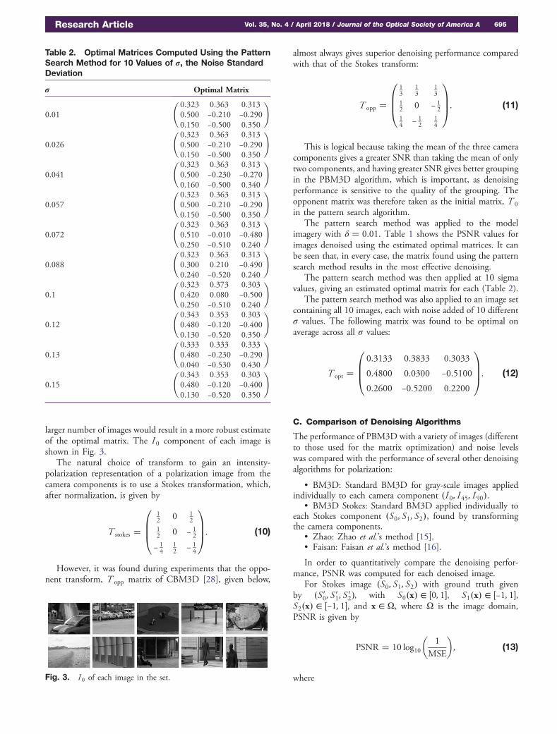
Figures 6–8 show the denoised images corresponding to theσ � 0.026 row of Table 3 as well as the ground truth and noisyimages. It can be seen that, as well as providing the greatestPSNR value, the visual quality of the images denoised usingPBM3D is the greatest of the methods tested. In all threefigures, the S0 component for the images denoised using

0.05 0.1 0.1520

30

40

50

PSN

R

oranges

0.05 0.1 0.1520

30

40

50

PSN

R

cars

0.05 0.1 0.1520

30

40

50

PSN

R

windows

0.05 0.1 0.1520

30

40

50

PSN

R

statue

BM3DBM3D StokesPBM3DZhaoFaisan

0.05 0.1 0.1520

30

40

50

PSN

R

carpark

0.05 0.1 0.1520

30

40

50

PSN

R

dogs

0.05 0.1 0.1520

30

40

50

PSN

R

courtyard

0.05 0.1 0.1520

30

40

50

PSN

R

mudflat

Fig. 4. PSNR for denoised images as a function of σ, the standard deviation of noise. Above each plot is the name of the image denoised; linecolors correspond to different denoising algorithms. For the top row, PSNR values are shown in Table 3. It can be seen that, for all images and allvalues of σ, PBM3D produces images with the greatest PSNR.

Table 3. PSNR for Denoising of Four Images (“Oranges,” “Cars,” “Windows,” “Statue”) Using Several Methods (B, BM3D;S, BM3D Stokes; P, PBM3D; Z, Zhao; F, Faisan) and Several Values of σ, the Standard Deviation of the Noise, Addeda

Oranges Cars Windows Statue

σ B S P Z F B S P Z F B S P Z F B S P Z F

0.010 47.3 48.3 49.0 34.7 45.6 45.6 46.4 47.0 28.4 43.0 44.8 46.1 47.1 24.5 42.1 45.2 46.5 47.3 26.9 42.50.026 43.4 44.2 44.9 34.7 41.8 40.4 41.2 41.9 28.4 37.5 39.1 40.5 41.5 24.5 35.4 40.1 41.4 42.1 26.9 36.40.041 41.5 42.3 43.0 34.6 39.9 38.0 38.9 39.5 28.4 35.2 36.3 37.7 38.8 24.5 32.5 37.7 39.0 39.6 26.9 33.70.057 39.8 40.7 41.5 34.4 38.1 36.3 37.2 37.9 28.3 33.5 34.4 35.8 36.9 24.5 30.6 35.8 37.2 37.9 26.9 32.10.072 38.5 39.5 40.5 34.3 36.9 34.9 35.8 36.6 28.3 32.4 33.0 34.4 35.5 24.4 29.4 34.4 35.9 36.7 26.9 31.10.088 37.4 38.4 39.4 34.0 35.8 33.9 34.8 35.7 28.2 31.5 31.8 33.2 34.3 24.4 28.4 33.3 34.8 35.6 26.8 30.10.103 36.6 37.7 38.7 34.0 34.9 33.0 34.0 34.8 28.2 30.8 31.0 32.4 33.4 24.3 27.6 32.3 33.8 34.6 26.8 29.60.119 35.8 37.0 37.9 33.8 34.2 32.3 33.4 34.1 28.1 30.2 30.1 31.3 32.5 24.4 26.8 31.5 33.1 33.9 26.8 29.00.134 35.0 36.4 37.1 33.4 33.5 31.6 32.7 33.3 28.1 29.7 29.4 30.7 31.6 24.3 26.2 30.8 32.4 33.1 26.7 28.60.150 34.4 36.1 36.2 33.3 33.0 31.2 32.4 32.5 28.0 29.3 28.9 30.2 30.6 24.3 25.7 30.3 31.9 32.2 26.7 28.3

aBold indicates greatest PSNR. It can be seen that PBM3D is always the best-performing method. The pattern continues with other images; the results (includingthose shown here) are plotted in Fig. 4.

696 Vol. 35, No. 4 / April 2018 / Journal of the Optical Society of America A Research Article

BM3D, BM3D Stokes, and PBM3D appear similar to theground truth, with the image denoised using Faisan appearingto be slightly less sharp. The S1 and S2 components of the im-ages denoised using BM3D and Faisan appear to have moredenoising artifacts than those denoised using BM3D Stokesand PBM3D. In the DoP components, the images denoised

using PBM3D have cleaner edges, which are more similar tothe ground truth than DoP components denoised using allof the other methods; this is highlighted in Fig. 9, which showsa close-up of the “window” images. The AoP componentsdenoised using PBM3D are notably more faithful to the

S0

G

S1

S2

S

P

Fig. 5. “Oranges” image with noise of standard deviation σ � 0.15(a high noise level), denoised using BM3D Stokes (S) and PBM3D (P)(G, ground truth). For BM3D Stokes and PBM3D, the S0 images arevisually similar to the ground truth. For both methods, however, theS1 images are notably different, and the S2 images are almost unrec-ognizable.

S0

G

S1

S2 DOP AOP

N

B

S

P

Z

F

Fig. 6. Polarization components of “oranges” image after applica-tion of several denoising methods. G, ground truth; N, noisy; B,BM3D; S, BM3D Stokes; P, PBM3D; Z, Zhao; F, Faisan. Noise stan-dard deviation, σ � 0.026. Note that the DoP images have beenscaled such that black represents DoP � 0 and white representsDoP � 0.5.

S0

G

S1

S2 DOP AOP

N

B

S

P

Z

F

Fig. 7. Polarization components of “cars” image after application ofseveral denoising methods. G, ground truth; N, noisy; B, BM3D; S,BM3D Stokes; P, PBM3D; Z, Zhao; F, Faisan. Noise standarddeviation, σ � 0.026.

S0

G

S1

S2

DOP AOP

N

B

S

P

Z

F

Fig. 8. Polarization components of “window” image after applica-tion of several denoising methods. G, ground truth; N, noisy; B,BM3D; S, BM3D Stokes; P, PBM3D; Z, Zhao; F, Faisan. Noise stan-dard deviation, σ � 0.026.

Research Article Vol. 35, No. 4 / April 2018 / Journal of the Optical Society of America A 697

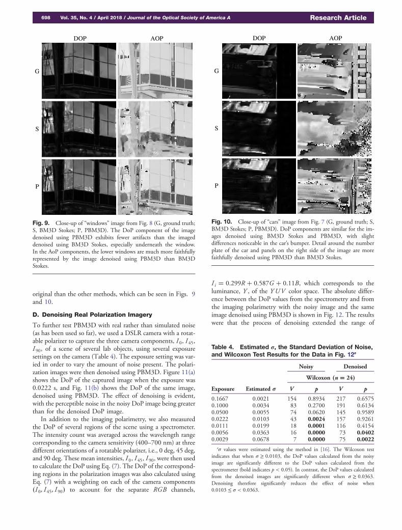
original than the other methods, which can be seen in Figs. 9and 10.

D. Denoising Real Polarization Imagery

To further test PBM3D with real rather than simulated noise(as has been used so far), we used a DSLR camera with a rotat-able polarizer to capture the three camera components, I 0, I 45,I 90, of a scene of several lab objects, using several exposuresettings on the camera (Table 4). The exposure setting was var-ied in order to vary the amount of noise present. The polari-zation images were then denoised using PBM3D. Figure 11(a)shows the DoP of the captured image when the exposure was0.0222 s, and Fig. 11(b) shows the DoP of the same image,denoised using PBM3D. The effect of denoising is evident,with the perceptible noise in the noisy DoP image being greaterthan for the denoised DoP image.

In addition to the imaging polarimetry, we also measuredthe DoP of several regions of the scene using a spectrometer.The intensity count was averaged across the wavelength rangecorresponding to the camera sensitivity (400–700 nm) at threedifferent orientations of a rotatable polarizer, i.e., 0 deg, 45 deg,and 90 deg. These mean intensities, I0, I 45, I 90, were then usedto calculate the DoP using Eq. (7). The DoP of the correspond-ing regions in the polarization images was also calculated usingEq. (7) with a weighting on each of the camera components�I0; I45; I 90� to account for the separate RGB channels,

I i � 0.299R � 0.587G � 0.11B, which corresponds to theluminance, Y , of the YUV color space. The absolute differ-ence between the DoP values from the spectrometry and fromthe imaging polarimetry with the noisy image and the sameimage denoised using PBM3D is shown in Fig. 12. The resultswere that the process of denoising extended the range of

DOP

G

AOP

S

P

Fig. 9. Close-up of “windows” image from Fig. 8 (G, ground truth;S, BM3D Stokes; P, PBM3D). The DoP component of the imagedenoised using PBM3D exhibits fewer artifacts than the imageddenoised using BM3D Stokes, especially underneath the window.In the AoP components, the lower windows are much more faithfullyrepresented by the image denoised using PBM3D than BM3DStokes.

DOP

G

AOP

S

P

Fig. 10. Close-up of “cars” image from Fig. 7 (G, ground truth; S,BM3D Stokes; P, PBM3D). DoP components are similar for the im-ages denoised using BM3D Stokes and PBM3D, with slightdifferences noticeable in the car’s bumper. Detail around the numberplate of the car and panels on the right side of the image are morefaithfully denoised using PBM3D than BM3D Stokes.

Table 4. Estimated σ, the Standard Deviation of Noise,and Wilcoxon Test Results for the Data in Fig. 12a

Noisy Denoised

Wilcoxon �n � 24�Exposure Estimated σ V p V p

0.1667 0.0021 154 0.8934 217 0.65750.1000 0.0034 83 0.2700 191 0.61340.0500 0.0055 74 0.0620 145 0.95890.0222 0.0103 43 0.0024 157 0.92610.0111 0.0199 18 0.0001 116 0.41540.0056 0.0363 16 0.0000 73 0.04020.0029 0.0678 7 0.0000 75 0.0022

aσ values were estimated using the method in [16]. The Wilcoxon testindicates that when σ ≥ 0.0103, the DoP values calculated from the noisyimage are significantly different to the DoP values calculated from thespectrometer (bold indicates p < 0.05). In contrast, the DoP values calculatedfrom the denoised images are significantly different when σ ≥ 0.0363.Denoising therefore significantly reduces the effect of noise when0.0103 ≤ σ < 0.0363.

698 Vol. 35, No. 4 / April 2018 / Journal of the Optical Society of America A Research Article

exposure time, over which the imaging polarimetric values werethe same as the spectrometry measurements. Table 4 demon-strates that, at an exposure time of 0.0222 s, when σ ≥ 0.0103,the values of the DoP from the noisy image become signifi-cantly different (Wilcoxon, n � 24, V � 43, p � 0.002) from

those calculated using the spectrometry measurements. In con-trast, when the images were denoised using PBM3D, the ex-posure time could be bought down to 0.0056 s (σ ≥ 0.0363)before the DoP values became different (Wilcoxon, n � 24,V � 73, p � 0.040). Therefore, denoising using PBM3D

1

2

34

5

6

7

8

9

10

11

12

13

14

15

16

17

18

19

20

2122

23

24

1

2

34

5

6

7

8

9

10

11

12

13

14

15

16

17

18

19

20

2122

23

24

(a)

(b)

Fig. 11. DoP image of a collection of lab objects, taken with an exposure of 0.0222s. (a) Image without denoising. (b) Image denoised usingPBM3D. The circles indicate where the true DoP value was measured using a spectrometer. It can be seen that the noisy image tends to show muchlarger DoP values. DoP values measured at each point are shown in Fig. 12.

Research Article Vol. 35, No. 4 / April 2018 / Journal of the Optical Society of America A 699

increases the accuracy of the measurements by reducing the ef-fect of noise on the measurement, allowing approximately 3.5times as much noise to be tolerated.

6. CONCLUSION

Imaging polarimetry provides additional useful informationfrom a natural scene compared with intensity-only imaging,and it has been found to be useful in many diverse applications.Imaging polarimetry is particularly susceptible to image degra-dation due to noise. Our contribution is the introduction of anovel denoising algorithm, PBM3D, which, when comparedwith state-of-the-art polarization denoising algorithms, givessuperior performance. When applied to a selection of noisy im-ages, those denoised using PBM3D had a PSNR of 4.50 dBgreater on average than those denoised using the method ofFaisan et al. [16] and 0.84 dB greater than those denoised usingBM3D Stokes. PBM3D relies on a transformation from cameracomponents into intensity-polarization components. We havegiven two algorithms for computing the optimal transforma-tion matrix and given the optimal for our system and dataset. We have also shown that, if imaging polarimetry is used toprovide DoP point measurements, denoising using PBM3Dallows approximately 3.5 times as much noise to be presentthan without denoising for the image to still have accuratemeasurements.

Funding. Engineering and Physical Sciences ResearchCouncil (EPSRC) (EP/I028153/1); Air Force Office ofScientific Research (AFOSR) (FA8655-12-2112).

Acknowledgment. The authors thank C. Heinrich andJ. Zallat for the use of their denoising code.

REFERENCES

1. E. Hecht, Optics (Addison-Wesley, 2002).2. G. Horváth and D. Varju, Polarized Light in Animal Vision: Polarization

Patterns in Nature (Springer, 2004).3. G. Horváth, ed., Polarized Light and Polarization Vision in Animal

Sciences (Springer, 2014).4. R. Wehner and M. Müller, “The significance of direct sunlight and

polarized skylight in the ant’s celestial system of navigation,” Proc.Natl. Acad. Sci. USA 103, 12575–12579 (2006).

5. M. J. How, M. L. Porter, A. N. Radford, K. D. Feller, S. E. Temple, R. L.Caldwell, N. J. Marshall, T. W. Cronin, and N. W. Roberts, “Out of theblue: The evolution of horizontally polarized signals in Haptosquilla(Crustacea, Stomatopoda, Protosquillidae),” J. Exp. Biol. 217,3425–3431 (2014).

6. M. J. How, J. H. Christy, S. E. Temple, J. M. Hemmi, N. J. Marshall,and N. W. Roberts, “Target detection is enhanced by polarizationvision in a fiddler crab,” Curr. Biol. 25, 3069–3073 (2015).

7. J. Taylor, P. Davis, and L. Wolff, “Underwater partial polarizationsignatures from the shallow water real-time imaging polarimeter(shrimp),” in OCEANS’02 MTS/IEEE (2002), pp. 1526–1534.

8. T. York, S. B. Powell, S. Gao, L. Kahan, T. Charanya, D. Saha, N. W.Roberts, T. W. Cronin, J. Marshall, S. Achilefu, S. P. Lake, B. Raman,and V. Gruev, “Bioinspired polarization imaging sensors: from circuitsand optics to signal processing algorithms and biomedical applica-tions,” Proc. IEEE 102, 1450–1469 (2014).

9. F. Snik, J. Craven-Jones, M. Escuti, S. Fineschi, D. Harrington, A. DeMartino, D. Mawet, J. Riedi, and J. S. Tyo, “An overview of polarimetricsensing techniques and technology with applications to differentresearch fields,” Proc. SPIE 9099, 90990B (2014).

10. W. de Jong, J. Schavemaker, and A. Schoolderman, “Polarizedlight camera; a tool in the counter-IED toolbox,” in Prediction andDetection of Improvised Explosive Devices (IED) (SET-117) (RTO,2007).

11. S.-S. Lin, K. Yemelyanov, E. N. Pugh, and N. Engheta, “Polarizationenhanced visual surveillance techniques,” in Proceedings of IEEEInternational Conference on Networking, Sensing and Control (2004),pp. 216–221.

12. D. Miyazaki and K. Ikeuchi, “Shape estimation of transparent objectsby using inverse polarization ray tracing,” IEEE Trans. Pattern Anal.Mach. Intell. 29, 2018–2029 (2007).

13. A. E. R. Shabayek, O. Morel, and D. Fofi, “Bio-inspired polarizationvision techniques for robotics applications,” in Handbook ofResearch on Advancements in Robotics and Mechatronics (IGIGlobal, 2015), pp. 81–117.

14. K. H. Britten, T. D. Thatcher, and T. Caro, “Zebras and biting flies:Quantitative analysis of reflected light from Zebra coats in their naturalhabitat,” PLoS ONE 11, e0154504 (2016).

15. Y.-Q. Zhao, Q. Pan, and H.-C. Zhang, “New polarization imagingmethod based on spatially adaptive wavelet image fusion,” Opt.Eng. 45, 123202 (2006).

16. S. Faisan, C. Heinrich, F. Rousseau, A. Lallement, and J. Zallat, “Jointfiltering estimation of Stokes vector images based on a nonlocalmeans approach,” J. Opt. Soc. Am. 29, 2028–2037 (2012).

17. A. Buades, B. Coll, and J. Morel, “A review of image denoisingalgorithms, with a new one,” Multiscale Model. Simul. 4, 490–530(2005).

18. K. Dabov, A. Foi, V. Katkovnik, and K. Egiazarian, “Image denoisingby sparse 3-d transform-domain collaborative filtering,” IEEE Trans.Image Process. 16, 2080–2095 (2007).

19. E. Collett, Field Guide to Polarization (SPIE, 2005).20. J. S. Tyo, D. L. Goldstein, D. B. Chenault, and J. A. Shaw, “Review of

passive imaging polarimetry for remote sensing applications,” Appl.Opt. 45, 5453–5469 (2006).

21. J. Zallat, S. Aïnouz, and M. P. Stoll, “Optimal configurations for imag-ing polarimeters: impact of image noise and systematic errors,” J. Opt.A 8, 807–814 (2006).

22. R.-Q. Xia, X. Wang, W.-Q. Jin, and J.-A. Liang, “Optimization ofpolarizer angles for measurements of the degree and angle of linearpolarization for linear polarizer-based polarimeters,” Opt. Commun.353, 109–116 (2015).

0 0.2 0.4 0.6 0.8 | n - s |

0

0.2

0.4

0.6

0.8

| d

- s

|

Fig. 12. Absolute value of the difference between DoP values mea-sured using the spectrometer and the noisy images, jn − sj, and spec-trometer and the denoised images, jd − sj. The noisy and denoisedimages had varying noise values, as given in Table 4. The locationswhere the DoP values were calculated are shown in Fig. 11. Black lineindicates where jd − sj � jn − sj; it can be seen that using the denoisedimages for DoP measurements results in much greater agreement withmeasurements taken using the noisy image as for most measurementsjd − sj < jn − sj. Table 4 uses this data to show that denoising signifi-cantly reduces the error due to noise.

700 Vol. 35, No. 4 / April 2018 / Journal of the Optical Society of America A Research Article

23. S. Chang, B. Yu, and M. Vetterli, “Spatially adaptive wavelet thresh-olding with context modeling for image denoising,” IEEE Trans. ImageProcess. 9, 1522–1531 (2000).

24. G. Sfikas, C. Heinrich, J. Zallat, C. Nikou, and N. Galatsanos,“Recovery of polarimetric Stokes images by spatial mixture models,”J. Opt. Soc. Am. 28, 465–474 (2011).

25. J. Valenzuela and J. Fessler, “Joint reconstruction of Stokes imagesfrom polarimetric measurements,” J. Opt. Soc. Am. A 26, 962–968(2009).

26. J. Zallat and C. Heinrich, “Polarimetric data reduction: a Bayesianapproach,” Opt. Express 15, 83–96 (2007).

27. H. Sadreazami, M. O. Ahmad, andM. N. S. Swamy, “A study on imagedenoising in contourlet domain using the alpha-stable family of distri-butions,” Signal Process. 128, 459–473 (2016).

28. K. Dabov, A. Foi, V. Katkovnik, and K. Egiazarian, “Color imagedenoising via sparse 3d collaborative filtering with grouping constraintin luminance-chrominance space,” in IEEE International Conferenceon Image Processing (2007), Vol. 1, pp. I-313–I-316.

29. A. Danielyan, A. Foi, V. Katkovnik, and K. Egiazarian, “Denoising ofmultispectral images via nonlocal groupwise spectrum-PCA,” inConference on Colour in Graphics, Imaging, and Vision (2010),pp. 261–266.

30. M. Maggioni, V. Katkovnik, K. Egiazarian, and A. Foi, “Nonlocal trans-form-domain filter for volumetric data denoising and reconstruction,”IEEE Trans. Image Process. 22, 119–133 (2013).

31. M. Maggioni, G. Boracchi, A. Foi, and K. Egiazarian, “Video denoising,deblocking, and enhancement through separable 4-D nonlocalspatiotemporal transforms,” IEEE Trans. Image Process. 21, 3952–3966 (2012).

32. M. Lebrun, “An analysis and implementation of the BM3D imagedenoising method,” Image Process. On Line 2, 175–213 (2012).

33. L. B. Wolff, “Polarization-based material classification from specularreflection,” IEEE Trans. Pattern Anal. Mach. Intell. 12, 1059–1071(1990).

34. Y. Y. Schechner, S. G. Narasimhan, and S. K. Nayar, “Polarization-based vision through haze,” Appl. Opt. 42, 511–525 (2003).

Research Article Vol. 35, No. 4 / April 2018 / Journal of the Optical Society of America A 701