© Copyright by Xiao Zhang 2016

LiDAR BASED CHANGE DETECTION FOR EARTHQUAKE SURFACE

RUPTURES

A Dissertation

Presented to

the Faculty of the Department of Civil and Environmental Engineering

University of Houston

In Partial Fulfillment

of the Requirements for the Degree of

Doctor of Philosophy

in Geosensing Systems Engineering and Sciences

by

Xiao Zhang

May 2016

LIDAR BASED CHANGE DETECTION FOR EARTHQUAKE SURFACE

RUPTURES

An Abstract

of a

Dissertation

Presented to

the Faculty of the Department of Civil and Environmental Engineering

University of Houston

In Partial Fulfillment

of the Requirements for the Degree of

Doctor of Philosophy

in Geosensing Systems Engineering and Sciences

by

Xiao Zhang

May 2016

vi

ABSTRACT

Determination of near-fault ground deformation during and after an earthquake is key to

understanding the physics of earthquakes. Observations with high spatial resolution and accuracy

of natural faults that have experienced earthquakes are required to understand the mechanism of

earthquake surface ruptures, which are presently poorly understood. Significant damage due to

earthquakes, coupled with poor comprehension of the patterns of uplifting, subsidence, and lateral

slipping of surface ruptures, requires the ability to rapidly characterize three-dimensional (3-D)

deformation over large areas to study stress change on faults and after-slip activity.

As Earth observation data becomes ubiquitous, remote sensing based change detection is

becoming more and more important for scientific applications, environmental policy and decision-

making. Light Detection and Ranging (LiDAR) is a proven approach to creating fast and accurate

terrain models for change detection applications. An Airborne LiDAR Scanning (ALS) system,

which combines a scanning laser with both GPS and inertial navigation technology, can create a

precise, three-dimensional set of points for features on the Earth’s surface.

Temporal differencing of repeat ALS surveys is a potential method for determining near field

surface deformation caused by earthquakes. Early studies have shown the potential of obtaining

displacement fields by differencing repeat LiDAR scans. However, the overall methodology has

not received sufficient attention and optimal methods of estimating 3-D displacement from ALS

are needed.

The primary contribution to knowledge presented in this dissertation is an experimental

evaluation of the performance of state-of-art 3-D registration methods for the determination of near-

fault earthquake deformation, including closest point criterion based and probability based 3-D

registration. Rigid and non-rigid algorithms are both taken into consideration to determine

vii

deformation. The convergence behavior, computational time and matching accuracy of every

method is assessed in terms of stability and robustness to transformation, noise level, and sampling

rate. Moreover, the best performing method is closely examined to determine the optimal scheme

and parameters used to autonomously estimate spatially varying earthquake introduced 3-D

displacements.

A new solution, the Anisotropic Iterative Closest Point (A-ICP) algorithm, has been

developed to overcome the difficulties associated with sparse legacy pre-event datasets. The

method incorporates point accuracy estimates to both speed up the Iterative Closest Point (ICP)

method and improve the matching accuracy. In addition, a new partition scheme, known as a

“moving window,” is proposed to handle the large spatial scale point cloud coverage over fault

zones and to enhance the change detection results for local, varying surface deformation near the

fault. Finally, to make full use of the multi-return and classified point clouds, the enhancement of

anthropogenic features in change detection is examined in near-fault displacement research.

viii

TABLE OF CONTENTS

ABSTRACT ------------------------------------------------------------------------------------------------------------- vi

TABLE OF CONTENTS ------------------------------------------------------------------------------------------- viii

LIST OF FIGURES ----------------------------------------------------------------------------------------------------- x

LIST OF TABLES ---------------------------------------------------------------------------------------------------- xv

1 INTRODUCTION ----------------------------------------------------------------------------------------- 1

1.1 EARTHQUAKE SURFACE DEFORMATION AND ITS RESEARCH SIGNIFICANCE -------------------- 1

1.2 CURRENT CHANGE DETECTION APPLICATIONS ON EARTHQUAKE SURFACE DEFORMATION -- 3

1.3 ALS DIFFERENCING ON EARTHQUAKE SURFACE DEFORMATION -------------------------------- 7

1.4 OBJECTIVES AND NOVEL CONTRIBUTIONS ------------------------------------------------------- 13

2 LIDAR BASED CHANGE DETECTION ----------------------------------------------------------- 17

2.1 AIRBORNE LIDAR (LIGHT DETECTION AND RANGING) ---------------------------------------- 17

2.2 LIDAR POINT CLOUD ------------------------------------------------------------------------------- 22

2.3 CHANGE DETECTION USING TEMPORAL SPACED LIDAR --------------------------------------- 24

2.3.1 1-D Slope-Based ------------------------------------------------------------------------------ 25

2.3.2 2-D Alignment for 3-D Point Clouds ------------------------------------------------------- 26

2.3.3 3-D Registration-Closest Point Criterion (CPC) Based --------------------------------- 29

2.3.4 3-D Registration - Probability-Based ------------------------------------------------------ 42

3 PERFORMANCE EVALUATION AND COMPARISON --------------------------------------- 49

3.1 ACCURACY CONTRIBUTION OF PROCEDURES BEFORE 3-D CHANGE DETECTION ------------ 49

3.1.1 Unification of Georeferencing Systems ---------------------------------------------------- 50

3.1.2 Accuracy of LiDAR Data Collection ------------------------------------------------------- 52

3.2 EVALUATION OF DIFFERENT REGISTRATION METHODS ----------------------------------------- 55

3.2.1 Test Datasets ---------------------------------------------------------------------------------- 57

ix

3.2.2 Evaluation of Registration Algorithms ----------------------------------------------------- 58

4 DETAILED EXAMINATION OF ICP --------------------------------------------------------------- 66

4.1 ICP REFINEMENTS ----------------------------------------------------------------------------------- 66

4.2 TEST DATASET --------------------------------------------------------------------------------------- 67

4.3 TEST RESULT AND DISCUSSION -------------------------------------------------------------------- 68

4.4 SOURCES AND MAGNITUDES OF ERROR ----------------------------------------------------------- 73

5 CASE STUDY ON SURFACE RUPTURES -------------------------------------------------------- 77

5.1 EL MAYOR EARTHQUAKE --------------------------------------------------------------------------- 77

5.1.1 Airborne Dataset Description --------------------------------------------------------------- 78

5.1.2 Methods ---------------------------------------------------------------------------------------- 79

5.1.3 Results & Discussion ------------------------------------------------------------------------- 80

5.2 SOUTH NAPA EARTHQUAKE ------------------------------------------------------------------------ 90

5.2.1 Airborne Dataset Description --------------------------------------------------------------- 92

5.2.2 Methods ---------------------------------------------------------------------------------------- 94

5.2.3 Results and Discussion ----------------------------------------------------------------------- 96

6 CONCLUSIONS AND FUTURE WORK ---------------------------------------------------------- 113

6.1 CONTRIBUTIONS OF DISSERTATION AND CONCLUSIONS ---------------------------------------- 113

6.2 FUTURE WORK -------------------------------------------------------------------------------------- 119

6.2.1 Improved ALS Differencing Techniques --------------------------------------------------- 119

6.2.2 Integration of ALS with Other Observations in Earthquake Physics ----------------- 121

REFERENCES ------------------------------------------------------------------------------------------------------- 123

x

LIST OF FIGURES

FIGURE 1 ESTIMATEDSPATIALRESOLUTIONANDSPATIALCOVERAGE (DISTANCE TO FAULT LINE)

OFCURRENT METHODSOFDETERMININGEARTHQUAKE SLIP, MODIFIED AFTER [54].FOR

CONTINUOUS IMAGERY SUCH AS SAR, PHOTOGRAPHY, AND LIDAR, THE HORIZONTAL AXIS

REPRESENTS SPATIAL COVERAGE, FOR SPARSE MEASUREMENTS, LIKE GPS AND FIELD DATA, THE

HORIZONTAL AXIS REPRESENTS DISTANCE TO THE FAULT LINE. ....................................................... 7

FIGURE 2 A TYPICAL ALS SYSTEM AND ITS MAJOR COMPONENTS. ............................................................... 17

FIGURE 3 A DIAGRAM SHOWING A PAIR OF OFFSET CROSS SECTIONS AND THE RELATIONSHIP BETWEEN

SYSTEMATIC HORIZONTAL AND VERTICAL OFFSET. ........................................................................ 25

FIGURE 4 AN ILLUSTRATION OF PIV (A FLOW VECTOR METHOD), USING THE CROSS-CORRELATION OF A PAIR

OF TWO SINGLY COLLECTED IMAGES............................................................................................. 28

FIGURE 5 ICP OVERVIEW SCHEME. ............................................................................................................... 30

FIGURE 6 2-D SCHEMATIC ILLUSTRATION OF (A) THE ORIGINAL ICP AND (B) THE A-ICP, AFTER [149]. ....... 41

FIGURE 7 DISPLACEMENTS FOR THE MW 6.0 AUGUST 2014 SOUTH NAPA EARTHQUAKE, DIFFERENCED FROM

PRE-EARTHQUAKE MEASUREMENTS AT SIX CGPS SITES USING 5-MINUTE KINEMATIC SOLUTIONS

(WHITE VECTORS) AND 24 HOUR SOLUTIONS (BLACK VECTORS). ERROR ELLIPSES REPRESENT 95%

CONFIDENCE [34]. ........................................................................................................................ 50

FIGURE 8 GEOMETRY FOR ALS POINT CLOUD GEOREFERENCING CALCULATION. ....................................... 52

FIGURE 9 TOTAL PROPAGATED UNCERTAINTY MAP FOR ALL THREE DIRECTIONS, (TOP) X, (MIDDLE) Y, AND

(BOTTOM) Z CONSIDERING ESTIMATED ACCURACY OF A RAW LIDAR SURVEY OVER THE

NORTHWESTERN (SIERRA CUCAPAH) SECTION OF THE EL MAYOR–CUCAPAH (EMC) EARTHQUAKE

SURFACE RUPTURE [13] . .............................................................................................................. 54

FIGURE 10 MODEL A: STANFORD BUNNY. ..................................................................................................... 58

FIGURE 11 MODEL B: NAPA SAMPLE. ............................................................................................................ 58

FIGURE 12 THE RESULTS FROM THE PAIRWISE REGISTRATION EXPERIMENTS WITH THE DIFFERENT ALGORITHMS

FOR MODEL A. ............................................................................................................................. 62

xi

FIGURE 13 THE RESULTS FROM THE PAIRWISE REGISTRATION EXPERIMENTS WITH THE DIFFERENT ALGORITHMS

FOR MODEL B, THE NAPA SAMPLE NEIGHBORHOOD. .................................................................... 63

FIGURE 14 (A) TOPOGRAPHY ALONG FLIGHT LINE #17, (B) SYNTHETIC LIDAR POINT ACCURACY, (C)

ARTIFICIAL SURFACE FAULT LINE CREATION. ................................................................................ 68

FIGURE 15 FLOW CHART FOR MOVING WINDOW A-ICP. THE BROWN BOX HIGHLIGHTS THE ITERATIVE

PROCESS TO DETERMINE THE OPTIMAL WINDOW SIZE AND STEP SIZE BY CONSIDERING THE DATA

DENSITY, THE NUMBER OF POINTS REQUIRED FOR AN ACCURATE ESTIMATION, AND THE EXPECTED

SPATIAL SCALE AND NATURE OF THE DEFORMATION. ..................................................................... 69

FIGURE 16 THE RESULTS FROM ICP AND A-ICP COMPARED WITH SYNTHETIC FAULT MOVEMENT. ................. 70

FIGURE 17 ALS POINT ACCURACY ESTIMATION FOR THE MILK POINT RIVER DATASET WITH SIMULATED RIGHT

LATERAL DISPLACEMENT. ............................................................................................................. 70

FIGURE 18 (A) RESULTS OF THE TILE-WISE ICP, (B) ER OF MOVING WINDOW A-ICP ESTIMATES, (C)

DIFFERENCES BETWEEN MOVING WINDOW ICP AND MOVING WINDOW A-ICP ESTIMATES, AND (D)

FINAL DISPLACEMENT ESTIMATE FROM MOVING WINDOW A-ICP. INSET FIGURE SHOWS

HORIZONTAL DISPLACEMENT VECTORS. ........................................................................................ 70

FIGURE 19 REFINEMENT OF NEAR-FAULT RUPTURE DISPLACEMENT. .............................................................. 71

FIGURE 20 POINT ACCURACY IN X (LEFT), Y (MIDDLE) AND Z (RIGHT), IN METERS, FOR THE PRE-EVENT EMC

EARTHQUAKE DATASET [13]. BOXES OVERLAID ON Y ACCURACY ESTIMATE SHOW APPROXIMATE

FLIGHT LINE EXTENTS FOR THE PRE-EVENT LIDAR DATASET. ...................................................... 80

FIGURE 21 MOVING WINDOW A-ICP ESTIMATES OF DISPLACEMENT FOR THE EMC EARTHQUAKE. (A) ER OF

LAST ITERATION, (B) DIFFERENCE BETWEEN MOVING WINDOW A-ICP AND MOVING WINDOW ICP

VERTICAL DISPLACEMENT ESTIMATES (C) FINAL MOVING WINDOW A-ICP ESTIMATE OF

HORIZONTAL SURFACE DISPLACEMENT IN X, (D) A-ICP ESTIMATE OF HORIZONTAL SURFACE

DISPLACEMENT IN Y, (E) A-ICP ESTIMATE OF VERTICAL SURFACE DISPLACEMENT IN Z, WITH

LOCATIONS OF MAJOR SURFACE RUPTURES AND PROFILES OVERLAID ON A-ICP ESTIMATE OF

VERTICAL SURFACE DISPLACEMENT, AND SCALE OF DISPLACEMENT FIELD IS INDICATED IN COLOR

SCALE FROM BLUE TO RED. ........................................................................................................... 83

xii

FIGURE 22 FOUR REPRESENTATIVE PROFILES OF THE ESTIMATED DISPLACEMENT FIELD IN HORIZONTAL

DIRECTION (DX AND DY), AND VERTICAL DIRECTION, DZ. STANDARD ICP (RED) AND MOVING

WINDOW A-ICP (BLUE). THE RED DOTTED LINES ON PROFILE CC’ AND DD’ SHOW THE SURFACE

DELINEATION IN ALL THREE COMPONENTS OF DISPLACEMENT AT THE LOCATION OF THE FAULT

RUPTURE, INDICATED BY THE RED ARROWS IN FIGURE 21. ............................................................ 84

FIGURE 23 FIELD TRANSECT PROFILE LOCATIONS OVERLAID ON THE A-ICP RESULTS OF VERTICAL

DISPLACEMENT. ............................................................................................................................ 86

FIGURE 24 DIFFERENCES BETWEEN ALS DIFFERENTIAL ESTIMATES AND EMC FIELD MEASUREMENTS AT THE

CORRESPONDING DISTANCE OF ICP WINDOW CENTER FROM LOCATIONS OF FIELD MEASUREMENTS

THE RUPTURE TRACE. ESTIMATED ACCURACY OF THE A-ICP ESTIMATES ARE GIVEN AS RED

(VERTICAL) AND BLUE (HORIZONTAL) BANDS IN THE FIGURE. THEY REPRESENT 1Σ VALUES. ....... 87

FIGURE 25 MAP SHOWING COSEISMIC AND POSTSEISMIC GNSS AND ALIGNMENT ARRAY RECORDS OF

DISPLACEMENT FROM THE AUGUST 24, 2014 EARTHQUAKE [199]. NOTE THAT THE NEAREST PBO

SITE, P261, IS LOCATED 11 KM FROM THE EPICENTER. .................................................................. 92

FIGURE 26 OVERVIEW OF THE STUDY AREA. LEFT IMAGE SHOWS STUDY REGION AND MAJOR FAULTS

SURROUNDING THE NAPA VALLEY EARTHQUAKE. RIGHT IMAGE DISPLAYS A DSM OF THE STUDY

AREA COMMON TO ALL ALS ACQUISITIONS, OVERLAID WITH A DEM OF BUILDINGS. THE YELLOW

SQUARE IS THE EXTENT OF THE BROWN’S VALLEY SUBURBAN AREA THAT IS THE FOCUS OF A

DETAILED ANALYSIS. .................................................................................................................... 93

FIGURE 27 POINT ACCURACY IN Y (CM) FOR THE 14J (LEFT) AND 14S (RIGHT) NAPA EARTHQUAKE DATASETS.

BOXES ON THE Y ACCURACY PLOT ESTIMATE FLIGHT LINE EXTENTS FOR THE PRE-EVENT LIDAR

DATASET. 96

FIGURE 28 A-ICP RESULTS OF NAPA AREA FOR 14S MINUS 14J. FROM TOP TO BOTTOM: CHANGE OF TERRAIN

ONLY AND THE TERRAIN AND GEODETIC MARKERS. FROM LEFT TO RIGHT: ESTIMATED

DISPLACEMENTS IN X, Y AND Z DIRECTIONS. ............................................................................... 98

FIGURE 29 A-ICP RESULTS OF DISPLACEMENTS OF BROWN’S VALLEY FOR 14S MINUS 14J IN X, Y AND Z

DIRECTIONS. FROM TOP TO BOTTOM: CHANGE OF TERRAIN ONLY, THE HISTOGRAM WITH MEAN AND

STANDARD DEVIATION (CM) OF ESTIMATED TERRAIN ONLY DISPLACEMENT ON EACH SIDE OF THE

xiii

WEST FAULT LINE (RED), CHANGE OF TERRAIN AND GEODETIC MARKERS, AND ITS HISTOGRAM OF

DISPLACEMENT ESTIMATED. ......................................................................................................... 99

FIGURE 30 A-ICP RESULTS OF DISPLACEMENTS OF THE NAPA AREA FOR 14J MINUS 03M IN X, Y AND Z

DIRECTIONS. FROM TOP TO BOTTOM: CHANGE OF TERRAIN ONLY, THE HISTOGRAM WITH MEAN AND

STANDARD DEVIATION OF ESTIMATED TERRAIN ONLY DISPLACEMENT ON EACH SIDE OF THE WEST

FAULT LINE, CHANGE OF TERRAIN AND GEODETIC MARKERS, AND ITS HISTOGRAM OF

DISPLACEMENT ESTIMATED. ....................................................................................................... 100

FIGURE 31 BOX PLOTS OF DEFORMATION ESTIMATED FOR 14S MINUS 14J. THE RESULTS FOR BROWN’S VALLEY

ARE SHADED IN LIGHT BLUE (LEFT) AND RESULTS FOR NAPA AREA ARE SHADED IN DEEPER BLUE

(RIGHT) FOR COMPARISON. THE BOX PLOTS OF TERRAIN ONLY CHANGE ARE IN BLUE AND TERRAIN

AND GEODETIC MARKER BOXPLOTS ARE IN BLACK. .................................................................... 101

FIGURE 32 A-ICP RESULTS OF DISPLACEMENTS OF NAPA AREA FOR 15 MINUS 14J IN THE X, Y, AND Z

DIRECTIONS. FROM TOP TO BOTTOM: CHANGE OF TERRAIN ONLY AND TERRAIN WITH GEODETIC

MARKERS. 103

FIGURE 33 A-ICP RESULTS OF DISPLACEMENTS OF NAPA AREA FOR 15 MINUS 14S IN THE X, Y, AND Z


MARKERS. 104

FIGURE 34 A-ICP RESULTS OF DISPLACEMENTS OF BROWN’S VALLEY FOR 15 MINUS 14J IN THE X, Y, AND Z


MARKERS. 104

FIGURE 35 A-ICP RESULTS OF DISPLACEMENTS OF BROWN’S VALLEY FOR 15 MINUS 14S IN THE X, Y, AND Z


MARKERS. 105

FIGURE 36 BOX PLOTS OF DEFORMATIONS ESTIMATED FOR 15 MINUS 14J. THE RESULTS FOR BROWN’S VALLEY


(RIGHT) FOR COMPARISON. THE BOX PLOTS OF CHANGE OF TERRAIN ONLY ARE IN BLUE AND

TERRAIN AND GEODETIC MARKERS ARE IN BLACK. ..................................................................... 105

xiv

FIGURE 37 BOX PLOTS OF DEFORMATIONS ESTIMATED FOR 15 MINUS 14S. THE RESULTS FOR BROWN’S VALLEY


(RIGHT) FOR COMPARISON. THE BOX PLOTS OF CHANGE OF TERRAIN ONLY ARE IN BLUE AND

TERRAIN AND GEODETIC MARKERS ARE IN BLACK. ..................................................................... 106

FIGURE 38 FROM TOP TO BOTTOM, THE BOX PLOTS OF DEFORMATIONS FOR THE ENTIRE NAPA EXTENTS

DECOMPOSED IN THE X, Y, AND Z DIRECTIONS. STATISTICS OF RESULTS FOR 14J MINUS 03M, 14S

MINUS 14J, 15 MINUS 14J, AND 15 MINUS 14J ARE GIVEN RESPECTIVELY. ................................... 107

FIGURE 39 TRANSECT PROFILES OVERLAY ON A-ICP RESULTS FOR 14S MINUS 14J. THE COLORED ESTIMATED

DISPLACEMENTS ARE CHANGE OF TERRAIN ONLY DISPLACEMENTS IN THE Y DIRECTION. ........... 109

FIGURE 40 HORIZONTAL OFFSETS BETWEEN ALS DIFFERENTIAL ESTIMATES USING 14S MINUS 14J AND FIELD

MEASUREMENTS, MARKED BY CIRCLE (TILE WISE ICP), ASTERISK (MOVING WINDOW ICP), AND

DIAMOND (MOVING WINDOW A-ICP), AT CORRESPONDING DISTANCE BETWEEN THE ICP WINDOW

CENTER AND LOCATIONS OF FIELD MEASUREMENTS (2014 AUGUST) ALONG THE RUPTURE TRACE.

109

FIGURE 41 PHOTOGRAPHS SHOWING A CHARACTERISTIC OF RIGHT-LATERAL FAULT DISPLACEMENT AT THE

GROUND SURFACE FEATURES RESULTING FROM FAULT DISPLACEMENT DURING THE NAPA

EARTHQUAKE. RIGHT-LATERAL DISPLACEMENT OF 40 CM WAS MEASURED NEAR THIS LOCATION

ONE DAY AFTER THE EARTHQUAKE. PHOTOGRAPH BY DAN PONTI, USGS [199]. ....................... 111

FIGURE 42 MEDIAN VALUE FINITE SLIP DISTRIBUTIONS (SDS) DERIVED FROM MONTE CARLO ANALYSIS FOR

THE NAPA VALLEY EARTHQUAKE. (A, B) PLAN AND MAP VIEW OF THE EAST-DIPPING FOCAL PLANE

(STRIKE 341°, DIP 80°) WITH OBSERVED (BLACK) AND MODELED (RED) CONTINUOUS GLOBAL

POSITIONING SYSTEM (GPS) DISPLACEMENTS [207]. ................................................................. 118

xv

LIST OF TABLES

TABLE 1. VARIATIONS OBSERVED IN THE EVALUATION DATASETS ................................................................ 60

TABLE 2 COMPARISON OF ICP AND A-ICP AGAINST REFERENCE MOVEMENT FOR FLIGHT LINE #17 AND

MOVING WINDOW ICP AND A-ICP AGAINST THE REFERENCE FOR THE ENTIRE DATASET (RESULTS IN

METERS). ...................................................................................................................................... 69

TABLE 3 SPECIFICATIONS OF THE PRE- AND POST-EVENT ALS DATASETS COVERING THE SURFACE RUPTURE

OF THE EMC EARTHQUAKE .......................................................................................................... 78

TABLE 4 SF6-1 FROM [197]. FIELD MEASUREMENTS OF SOUTH NAPA SURFACE RUPTURE. ......................... 87

TABLE 5 THE STATISTICS OF DIFFERENCES BETWEEN ALS DIFFERENTIAL ESTIMATES USING TILE WISE ICP,

MOVING WINDOW ICP, AND MOVING WINDOW A-ICP RESULTS AND FIELD MEASUREMENTS OF

DISPLACEMENT FROM THE EMC EARTHQUAKE. ........................................................................... 88

TABLE 6 SIGNIFICANT DATA ACQUISITION PARAMETERS FOR THE TWO PRE-EVENT AND TWO POST-EVENT

ALS COLLECTIONS FOR THE MW 6.0 AUGUST 2014 NAPA EARTHQUAKE. ..................................... 93

TABLE 7 THE STATISTICS OF DIFFERENCES BETWEEN ALS DIFFERENTIAL ESTIMATES USING TILE WISE ICP,

MOVING WINDOW ICP, AND MOVING WINDOW A-ICP AND FIELD MEASUREMENTS OF THE NAPA

EARTHQUAKE FOR BOTH 14S MINUS 14J AND 15 MINUS 14J. ...................................................... 111

1

1 INTRODUCTION

1.1 Earthquake Surface Deformation and Its Research Significance

The ground beneath our feet usually seems solid and unmoving, but on rare occasions, the

ground moves violently, causing catastrophic loss of life as buildings collapse and the Earth’s

surface is disrupted. These ground motions, known as earthquakes, are naturally occurring, broad-

banded vibratory ground motions. They originate in the rocky interior of the earth by tectonic

processes that rapidly release built up stress. Near tectonic plate boundaries an area of the crust

may first bend and then, when the stress exceeds the strength of the local crust, break or slip along

a plane of weakness, known as a fault or fracture, to a new position [1]. The earthquake energy

rapidly expands outward from the source, through the surrounding crust, to reach and shake the

Earth’s surface [2].

A fault is a fracture in the Earth's crust along which two blocks of crust have slipped with

respect to each other. Faults are divided into three main groups depending on how they move:

normal, thrust and strike-slip. Normal faults occur in response to pulling or tension; the overlying

block moves down the dip of the fault plane. Thrust (reverse) faults occur in response to squeezing

or compression; the overlying block moves up the dip of the fault plane [1]. Strike-slip faults are

vertical (or nearly vertical) fractures where the predominant block motion is horizontal. If the block

opposite an observer looking across the fault moves to the right, the slip style is termed right lateral;

if the block moves to the left, the motion is termed left lateral [3].

How do faults slip? Answering this question is one of the grand challenges in seismology [4].

Recent observations have revealed a rich spectrum of fault behavior, ranging from steady sliding

to earthquakes that can slide at super sheer velocities and emit shock waves that cause exceptionally

damaging ground motions [4]. Only in the past decade has it been discovered that major parts of

2

some fault systems slip repeatedly in slow events that occur surprisingly regularly and are

accompanied by low-amplitude seismic tremor. The migrating tremor during a 2- to 3- week

episode of slow slip on the Cascadia subduction zone [5] is an example of this type of activity.

There are many other questions regarding plate motion that still need to be addressed. For instance,

what is the relationship between episodic slip and tremor and major earthquakes? The rate and

distribution of fault slip is a crucial piece in understanding fault zone rheology [6], the relationship

between the stresses and the resulting deformation or strains, and in providing fundamental

constraints on earthquake processes.

Another important consideration is how near-fault surface material properties influence the

location and severity of earthquake hazards. The behavior of near-fault deformation can reveal the

nature of material properties that are affected by water, energy resources, and mineral resources at

depths of meters to a few kilometers [4]. By definition, near-fault deformation is motion that is

within ~20 km of a fault [6]. However, this definition is not universal. Accurate models of near-

fault surface deformation are needed in order to relate slip at depth to surface ruptures, to

understand the geometry of faulting in earthquakes, and to characterize seismic hazards [7] [8].

However, near-fault effects attenuate with increasing distance, which, in turn, makes it more

difficult to determine factors such as magnitude and local site conditions for ground motion with

far-field observations [9]. Detailed knowledge of near-fault deformation is, therefore, a crucial part

of seismology. Quantifying the extent and rate of near-fault surface deformation and plate

movement, can describe the stresses on faults. A stress distribution and temporally and spatially

dependent rheology is necessary to unravel the physics of earthquakes and determine which faults

are most likely to produce the next earthquake [10], [11]. For instance, the great Sumatra earthquake

of April 11, 2012, a massive magnitude of Mw 8.6 earthquake, set off a series of earthquakes around

the world that lasted for six days after the initial event [12] .

3

Observations made on natural faults that have experienced earthquakes are needed. Massive

damage from earthquakes, coupled with a poor understanding of uplifting and subsidence patterns,

necessitate 3-D surveys of larger areas with more detailed information to describe stress change on

faults as well as after-slip activities, rather than the sparsely distributed sample points that have

been used for decades [13]. Large earthquakes produce complex patterns of surface deformation,

therefore high accuracy and precision measurements are demanded to understand the mechanics of

earthquake surface ruptures because they reveal more topographic detail and allow more accurate

quantification of surface deformation [14].

Since the problem of determining coseismic deformation in the near-field of an

earthquake is relevantto both earth science, hazards research, andhazardmitigation in the event

of catastrophic earthquakes, surveying methods with low repeat times and rapid collection are

preferable to those that demand continuous maintenance and repeated visits. Rapid collection will

also improve earthquake early warning and rapid response [15].

1.2 Current Change Detection Applications on Earthquake Surface

Deformation

Earthquake surface deformation estimation is heavily data driven. To measure the motions

of the Earth’s surface, a variety of methods have been employed in both laboratory experiments

and field observations. Laboratory experiments have included the geological investigation of active

and inactive faults, physical and chemical features obtained by the field samples as well as

seismological estimation from seismic waveforms [16]. Field observations include creep meters

[17], alignment arrays, Global Positioning Systems (GPS), and seismic measurements. In the late

1960s, the USGS installed 25 alignment arrays along the creeping segment of the San Andreas

Fault. Each array consisted of between 8 and 20 benchmarks, was oriented approximately

perpendicular to the active trace of the San Andreas Fault, ranged in length from 30 to 200 m [18],

4

and was designed to be surveyed with a theodolite. Global Positioning System (GPS) data

measurements and continuously operating reference stations (CORS) were implemented for

measuring crustal motion in the 1980s [19]–[22]. In 1987, the USGS began using GPS in

earthquake-prone areas in California, including the region along the San Andreas Fault and around

San Francisco Bay. GPS technology and data analysis, unlike theodolite data, is ubiquitous and

thus establishes a basis for future measurements. Furthermore, differential GPS techniques allow

for unambiguous determination of horizontal and vertical deformation near the fault and facilitate

ties to an external reference frame if required.

Seismic waveform observations are also used to determine the fault rate and slip distribution

caused by earthquakes [23]–[25]. Near-source displacement seismograms are well adapted to

recording the dynamic and static parts of strong ground motions. The low-frequency parts of the

seismic waveform signals, in the time domain, are inverted to obtain information about the fault

orientation and the slip direction [25]. To infer the time-space evolution of slip [26]–[30], records

of coseismic ground displacement and ground acceleration from the above techniques are used.

However, discrepancies remain among those published results, e.g., the San Andreas Fault and the

eastern California shear zone has a well-documented and significant discrepancy between geologic

right-lateral strike-slip rates (e.g., [31]; [32]). Some inverse models use both GPS velocities and

geologic slip rates to constrain deformation within the southern California fault system,

consequently reducing the discrepancy between geologic slip rates and inversion-produced rates

[33] [34].

The major challenge for a geodetic model of near-fault deformation that uses conventional

field observation techniques is to exploit the spatially sparse data collection, such as the

observations from continuously operating reference stations (CORS) [35]. Some of the variations

are lost after the interpolation due to the extremely spatially sparse and non-uniform data samples.

Even the dense Plate Boundary Observatory (PBO) network [36], which is a geodetic

5

observatory designed to study the three-dimensional strain field resulting from deformation across

the active boundary zone between the Pacific and North American plates in the western United

States, hasaspatialresolutionon theorderof10-20km at best.Abnormal (non-physical)

gap areas are inevitably introduced due to modelling that utilizes a sparse data collection. “These

observations point to the need for field geologists to oversample displacement data after an

earthquake, rather than perform random, widely spaced measurements that may not represent the

actual coseismic slip distribution [37].” However, these datasets can be time consuming and

expensive to develop if high resolution is necessary.

In-field observations are key to providing ground truth measurements, but the shortcomings

of these observations have made quantification of near-field surface slip distributions surprisingly

subjective [38]. Modern remote sensing [39] techniques can provide crucial information to

compensate for the shortcomings of conventional field measurements. Emerging remote sensing

techniques in recent decades have been applied to map earthquake-related surface deformation,

construct base maps and tectonic frameworks that bridge the disciplines of seismology, structural

geology, and rock mechanics, and improve our understanding of geological phenomenon spatially

and temporally. These techniques include aerial and satellitepan-chromatic (e.g., SPOT) images,

Interferometric Synthetic Aperture Radar (InSAR), and airborne laser scanning (ALS) or airborne

Light Detection And Ranging (LiDAR). In parts of the U.S. with few or no historically-recorded

major earthquakes, or where background seismicity is sparse, remotely sensed geodetic data may

provide the only insight into present-day seismic hazards [40], [41].

Satellite geodetic techniques, such as Interferometric Synthetic Aperture Radar (InSAR),

enable imaging of the relative change of ground deformation with high resolution and wide

coverage soon after the event. This technique relies on the calculation of the interference pattern

caused by the difference in phase between two images acquired by a space-borne synthetic aperture

radar at two distinct times [42]. The resulting interferogram is a contour map of the change in

6

distance between the ground and the radar instrument along the radar line of sight. Its utility has

been compared to standard seismic inversion in inferring fault parameters such as epicenter depth,

location, focal mechanism [43], and uncertainty (+/-5 km with Moment Magnitude (Mw) > 5.5).

InSAR is a valuable source for observations of far-field deformation especially in near-vertical,

strike-slip faults [44]–[47], and provides a valuable indication of slip at depth. However, InSAR

near-field observations are inhibited due to the spatial symmetry in deformation fields and radiation

patterns of moderately sized, buried, strike-slip earthquakes [48]. Furthermore, InSAR is hindered

by coverage incoherence between flights; consequently, there is often a critical observational gap

between measurements taken at the fault scarp and those in the far-field [49]. Therefore ground

motion simulations have been the only viable way to obtain time histories for structural analysis of

near-fault deformation for decades because there are few actual ground motions recorded close to

ruptured faults; gaps close to surface faulting can only be compensated for through modelling and

data interpolation [50], [51].

Image based optical matching yields 2-D deformation nearthefault and over wide areas

and techniques include Co-Registration of Optically Sensed Images and Correlation (COSI-Corr)

[52], [53]. Theoretically, image-based methods can detect to the level of sub-pixel 2-D deformation.

For aerial photography, this means sub-meter to meter level and for satellite imagery it means meter

to tens of meters level. However, the technique is limitedtohorizontal grounddisplacement and

suffers from poor performance in homogeneous regions of the image where it is difficult for the

correlations process to establish the correct match. This makes it clearly unrealistic and insufficient

for geological observations in the near-fault region, especially when there are few inhomogeneous

ground features in the local area.

ALS has the capacity to address some of the shortcomings of other methods in the

earthquake rupture near‐field. The technique employs an aircraft‐mounted laser to measure sub‐

decimeter 3-D surface topography at a decimeter to centimeter spatial resolution. Spatial coverage

7

of ALS isdetermined by the width of the survey corridor, which can extendno more than a few

kilometers from either side of the fault line. For the purpose ofearthquake slip determination, ALS

data from a survey prior to an earthquake can becompared with data from one or several post‐

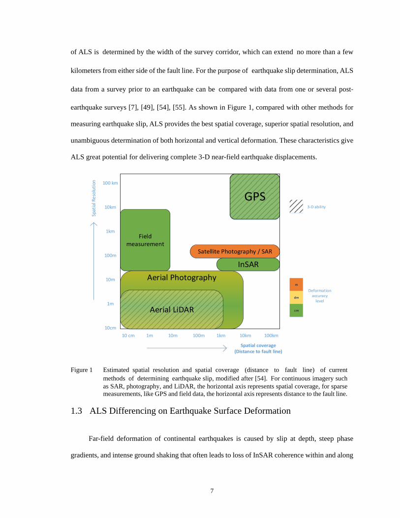
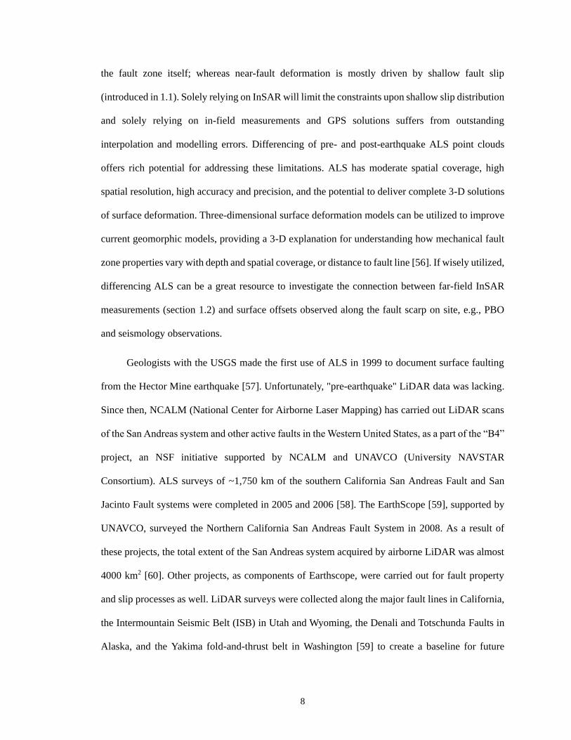
earthquake surveys [7], [49], [54], [55]. As shown in Figure 1, compared with other methods for

measuring earthquake slip, ALS provides the best spatial coverage, superior spatial resolution, and

unambiguous determination of both horizontal and vertical deformation. These characteristics give

ALS great potential for delivering complete 3-D near-field earthquake displacements.

Figure 1 Estimatedspatialresolutionandspatialcoverage (distance to fault line) ofcurrent

methodsofdeterminingearthquake slip, modified after [54].For continuous imagery such

as SAR, photography, and LiDAR, the horizontal axis represents spatial coverage, for sparse

measurements, like GPS and field data, the horizontal axis represents distance to the fault line.

1.3 ALS Differencing on Earthquake Surface Deformation

Far-field deformation of continental earthquakes is caused by slip at depth, steep phase

gradients, and intense ground shaking that often leads to loss of InSAR coherence within and along

GPS

Field measurement

Aerial Photography

Satellite Photography / SAR

InSAR

Aerial LiDAR

10 cm 1m 10m 100m 1km 10km 100km

100 km

10km

1km

100m

10m

1m

10cm

m

dm

cm

3-D ability

Spatial coverage(Distance to fault line)

Spat

ial R

eso

luti

on

Deformation accuracy

level

8

the fault zone itself; whereas near-fault deformation is mostly driven by shallow fault slip

(introduced in 1.1). Solely relying on InSAR will limit the constraints upon shallow slip distribution

and solely relying on in-field measurements and GPS solutions suffers from outstanding

interpolation and modelling errors. Differencing of pre- and post-earthquake ALS point clouds

offers rich potential for addressing these limitations. ALS has moderate spatial coverage, high

spatial resolution, high accuracy and precision, and the potential to deliver complete 3-D solutions

of surface deformation. Three-dimensional surface deformation models can be utilized to improve

current geomorphic models, providing a 3-D explanation for understanding how mechanical fault

zone properties vary with depth and spatial coverage, or distance to fault line [56]. If wisely utilized,

differencing ALS can be a great resource to investigate the connection between far-field InSAR

measurements (section 1.2) and surface offsets observed along the fault scarp on site, e.g., PBO

and seismology observations.

Geologists with the USGS made the first use of ALS in 1999 to document surface faulting

from the Hector Mine earthquake [57]. Unfortunately, "pre-earthquake" LiDAR data was lacking.

Since then, NCALM (National Center for Airborne Laser Mapping) has carried out LiDAR scans

of the San Andreas system and other active faults in the Western United States, as a part of the “B4”

project, an NSF initiative supported by NCALM and UNAVCO (University NAVSTAR

Consortium). ALS surveys of ~1,750 km of the southern California San Andreas Fault and San

Jacinto Fault systems were completed in 2005 and 2006 [58]. The EarthScope [59], supported by

UNAVCO, surveyed the Northern California San Andreas Fault System in 2008. As a result of

these projects, the total extent of the San Andreas system acquired by airborne LiDAR was almost

4000 km2 [60]. Other projects, as components of Earthscope, were carried out for fault property

and slip processes as well. LiDAR surveys were collected along the major fault lines in California,

the Intermountain Seismic Belt (ISB) in Utah and Wyoming, the Denali and Totschunda Faults in

Alaska, and the Yakima fold-and-thrust belt in Washington [59] to create a baseline for future

9

earthquakes along these known active fault zones. These results also support ongoing tectonic and

paleoseismic research. A great investment has been made in ALS data acquisition in fault zones

and earthquake prone areas in the past decade, resulting in an explosion in the amount of available

LiDAR data.

The growing investment in collections of pre- and post-event ALS datasets over earthquake

fault zones has created a wealth of observations that enable detailed documentation and study of

surface displacement with decimeter level resolution and accuracy. Furthermore, as the systems

improve, data quality will continue to increase. Modern LiDAR surveys can map wide regions at

point densities of several to tens of points/m2 or higher. Consequently, digital topographic surface

models (DSM) in seismogenic analysis, generated from LiDAR point clouds, are greatly improved

with minimal loss of spatial coherence because of the higher accuracy and precision of the

interpolation models. High resolution topographic surface models along fault zones are important

aids in the delineation of recently active breaks. LiDAR data, such as that collected in the B4 project,

of the San Andreas and San Jacinto fault zones in southern California [61] have densities of 3–4/m2

and can be gridded to between 0.25 and 0.5 m resolution using local binning with inverse distance

weighting and using a search radii of 0.8 m or larger. Those resolutions depict the tectonic

landforms at paleoseismic sites well enough to assess them with confidence. LiDAR surveys can

also record multiple returns from a single laser pulse, such as from vegetation and the underlying

ground surface; this capability allows the canopy to be removed from the LiDAR point clouds and

has been used to reveal previously unidentified fault scarps in densely forested regions. For instance,

in the forested mountainous terrain of the south-eastern Alps, Slovenia, a tree removal algorithm

was applied to the ALS mapping of seismogenic faults and the resulting images revealed surface

scarps and tectonic landforms in unprecedented detail [62]. The capability of LiDAR to penetrate

vegetation has the potential to reveal topographical features at higher levels of detail than would

otherwise be possible and has led to exciting advances, such as the archaeological discovery of

10

ancient structures in the Honduran jungle that were underneath dense vegetation [60], [63]. Point

spacing is getting finer than the scale of slip and displacement in large earthquakes. As a result,

differencing of ‘before’ and ‘after’ fault zone topography can reveal the “near-complete rupture”

[49], i.e., 3-D coseismic and postseismic surface displacements, given the 3-D nature of the data.

Nissen et al. (2012) first presented the method of applying a rigid body transformation algorithm

to determine three-dimensional (3-D) coseismic surface displacements and rotations by

differencing pre- and post-earthquake ALS point clouds [7], [49]. The approach has been applied

to ALS mapping on the San Andreas Fault as well as densely-vegetated sections of the June 14,

2008 Iwate–Miyagi ( Mw 6.9) and April 11, 2011 Fukushima–Hamadori ( Mw 7.1) earthquake

ruptures [49].

LiDAR differencing, similar to the method of Nissen et al. (2012), although a relatively new

field of investigation, has significantly advanced research in active tectonics and earthquake

geology [7], [13], [49], [64], [65]. However, demonstration of this emerging application for ALS

has so far been restricted by the lack of high quality paired datasets on which to test the

methodology. For example, the 2010 El Mayor–Cucapah earthquake rupture in northern Mexico is

one of the few earthquakes with complete pre- and post-LiDAR coverage but 3-D analysis of the

deformation field is made difficult by the unusually sparse density (∼0.013 points/m2) of the pre-

event dataset [55] [64]. Experiments on southern California LiDAR datasets deformed with

simulated earthquakes of known displacements reveal what could be possible with higher density

paired point clouds [7], [54]. In addition, these studies focus on semi-arid landscapes where

vegetation cover is not a serious issue. Other research in highly vegetated areas shows significant

noise (at a roughly ±50 cm level) but still yields valuable information about near-field deformation

and shallow fault slip [49]. Researchers in this field are actively looking for historical data from

other agencies, including LiDAR surveys, field measurements via PBO, seismic waveform data,

11

and satellite-based InSAR imagery, to compensate for the absence of pre-event LiDAR of

comparable quality to use in LiDAR differencing studies [66], [67].

Effective LiDAR-based differential analyses can make use of the wealth of LiDAR surveys

in earthquake fault zones. However, to date there are only a couple of examples of 3-D LiDAR

deformation detection applications [7], [49], [55] and they use either simple vertical only

differencing, i.e., DSM-based, or horizontal only differencing, i.e., image correlation methods. As

DSM differencing neglects the effect of lateral motion, the resulting elevation changes may not

correspond correctly to surface displacements, e.g., with the presence of slope, horizontal motion

can contribute to vertical displacement as well [68]. Image-correlation methods use image co-

registration processing techniques to estimate horizontal displacement between datasets.

Mukoyama (2011) presents an example of this type of analysis using particle image velocimetry

(PIV), a direct cross-correlation algorithm, to find correspondence between two slope gradient

images derived from the gridded DSMs in order to obtain horizontal displacements across the study

area and measure the lateral motions during an earthquake [69]. In [70] , another image-correlation

method called COSI-Corr developed by Leprince (2007) [71] was applied to a time-series of

LiDAR data acquired above the White Sand Dunes, NM, to derive the sand dune migration field

from 2007 to 2010 with ‘sub-pixel’ accuracy. ‘Sub-pixel’ refers to the unit size of an image cell

generated from the interpolation of LiDAR point clouds. DSM differencing and image-correlation

based methods require gridding or smoothing of one or both datasets, an additional step which can

potentially introduce biases or artefacts into the estimated displacement field.

3-D alignment overcomes the above issues with 2-D differencing by directly determining 3-

D surface displacements from raw LiDAR point clouds. The Iterative Closest Point (ICP) rigid

body transformation [72] algorithm is a technique for registering 3-D images that is widely used in

medicine, as a way of aligning and comparing multi-temporal scans of a subject’s body [73],

computer graphics [74], and robotics [75]. In the Earth sciences, it is the primary 3-D registration

12

method that has been implemented for landslide monitoring and co-seismic tectonic deformation

[7], [49], [64]. However, systematic evaluation of registration stability and robustness under

different testing scenarios and data characteristics (e.g., point density and precision) are absent from

the current research. The rationalization of ICP variants and parameters also needs to be examined

in more detail because ICP is not a perfect solution, it requires a good initial alignment or it can

easily fall into a local minimum, and the implementation of ICP is highly data oriented. For example,

in Earth surface deformation, ICP is often hindered the sparse density of pre-event data, as was the

case for the 2010 El Mayor–Cucapah earthquake pre- event data (∼0.013 points/m2) [55], [76].

Thus the application scheme and parameters used for each stage of analysis needs to consider the

unique event data available. Other than the limited implementation of ICP, little research has been

done to examine alignment methods in 3-D LiDAR-based earthquake deformation, leaving many

open questions. Current research has focused mainly on the validation of the technology through

accuracy assessments [77]–[80] or on the evolution of fault line trends as a result of major

earthquakes [54], [55]. Challenges still exist in registering point clouds, evaluating methods,

optimizing scales and spatial resolution, the use of complex topography, and applying spatial

statistics to characterize the effectiveness of the results. For example, if the data is irregularly

spaced, we can rasterize it in order to get regularly spaced data (voxel data [81], [82] ), but the

required accuracy for near-fault deformation may be lost. There can be large mismatches in point

density, particularly when comparing newer data to older data collected a number of years prior.

There may also be large errors in absolute point positioning, for instance, at the edges of scan lines,

as evidenced in the El Mayor dataset [64].

With the number of existing applications, there are still gaps remaining to be exploited in

LiDAR differencing as it pertains to earthquake deformation. These include:

a) Most of the literature only provides a comparison of pre- and post-earthquake fault

zone deformation. There has not been a systematic comparison and evaluation of the

13

effectiveness of existing LiDAR-based change detection methods. The lack of uniform

performance evaluation criteria is part of the problem.

b) Although previous research [7], [64] pointed out that performance differs with

varying surface conditions, such as vegetation coverage and topography, spatial

correlation analysis between surface conditions and differencing performance has not

been conducted so far.

c) Some methods require gridding or smoothing of one or both datasets, an additional

step that could introduce biases or artefacts in the resulting displacements and has not yet

been quantified.

d) Most of the previous approaches incorporated only elevations and some limited use

of LiDAR return intensities. They have not investigated the use of LiDAR point positions

relative to neighborhood points or LiDAR accuracy, which varies from point to point, and

can potentially be exploited for nonhomogeneous change detection.

e) There is also a lot of potential in multiple return LiDAR datasets that has not been

fully explored. This data could help reveal the near-field surface deformations around

faults. Most research has focused only on returns from the terrain and ground surface, but

returns from anthropogenic features, such as buildings, can also provide detailed

deformation information to describe near-fault movement.

1.4 Objectives and Novel Contributions

The principal objective of this dissertation is to examine the ability of ALS to recover small

magnitude surface displacements over large spatial scales and to evaluate the spatial resolution and

accuracy of these displacements using ALS datasets. The ground motion captured by the

measurement techniques should be able to provide vital information on the tectonic motions

between the earth’s plates (background motion), the offsets across a fault during a large earthquake

14

(the coseismic displacements), and the rapidly decaying motions that persist for weeks to years

after a large earthquake (after-slip).

To sum up, the goal of this study is to determine methods and parameters that can be used to

autonomously estimate spatially varying earthquake introduced 3-D displacements. To achieve this

goal, the following contributions will be shown:

1. Study of primary 3-D registration methods.

Principles of representative primary 3-D registration methods will be studied. Rigid

body registration, such as ICP and improvements on ICP, and non-rigid body registration

will be investigated to estimate movement in the displacement field. Experiments on

LiDAR datasets deformed with known movement and synthetic noise, to simulate actual

earthquake deformation, will be used to test 3-D deformation detection methods and show

what should be possible with higher density point clouds. Essentials of this research will

cover the following points:

a) Error contribution in the data collection phase, including the unification of

georeferencing systems and the horizontal/vertical datum used, LiDAR point error

propagation, and point accuracy estimation, will be discussed.

b) An evaluation of 3-D change detection techniques will be presented. Different

techniques will be analyzed and evaluated with a set of uniform performance

measurements, including registration accuracy, number of iterations, and computing time.

The performance of every algorithm will be assessd under different simulation senarios

in order to evaluate their robustness and stability to changes in point density, magnitude

of displacement, noise level, and sampling rate.

c) A detailed examination of the optimal method will be performed. The optimal

parameters and algorithm scheme for the best method from the previous evaluation will

be investigated. This will include tests of surveyed surface conditions, such as point

15

spacing, filtering, window size, type of observations (building or terrain), and anisotropic

noise.

2. Near-fault deformation studies using ALS-based 3-D registration method.

Possible methods to mitigate the difficulties associated with sparse legacy pre-event

datasets and the issues caused by anthropogenic change hidden in near-fault displacement

results are presented through two case studies. Results of the proposed methods using point

accuracy estimation will be presented. Anthropogenic change of the landscape will also be

analyzed and possible methods to make full use of the multi-return and classified point

cloud to enhance deformation determination will be presented.

a) In scenarios with large disparity in point density and accuracy, any surface-based

matching approach would not give ideal results because surface generation, usually in the

form of gridding, results in the loss of information from the denser dataset. A series of

improvements to standard ICP are applied in order to incorporate a point accuracy model

and overcome the disparity between pre- and post-event datasets. The approach works

well for remote and/or arid areas that would not be expected to have significant landscape

change between LiDAR surveys. The results show that less noise and more detail are

observed from this improved ICP technique, known as moving window A-ICP. The A-

ICP technique also appears to outperform ICP in handling the banded error pattern caused

by increased uncertainty at the edge of the pre-event ALS swaths.

f) In urban and agricultural areas, where anthropogenic change of the landscape is

expected and the surface displacements are smaller, e.g., less than the magnitude of 1

meter, any approach with sparse on site measurements would not give sufficient

information to provide a complete 3-D mapping with localized small-scale changes. The

proposed moving window A-ICP is applied in order to explore the ability of ALS to

recover small surface displacements near the spatial resolution of the ALS datasets.

16

Possible methods are investigated to mitigate problems in urban areas through the use of

urban geodetic markers, analogous to the persistent scatterer technique employed with

differential radar observations, by making use of the multi-return and classified point

cloud to resolve the anthropogenic change of the landscape hidden in near-fault

earthquake deformation.

17

2 LIDAR BASED CHANGE DETECTION

2.1 Airborne LiDAR (Light Detection And Ranging)

Airborne LiDAR (Light Detection And Ranging) is an active remote sensing technique that

uses short pulses of laser radiation to measure the range between a sensor and a target. It can be

used at night, reducing disruption to routine air traffic, and it can be flown under high cloud

conditions. Airborne LiDAR systems can be classified based on application (atmospheric, mapping,

bathymetry, navigation), the ranging technique (time of flight, triangulation, phase difference), the

target detection principle (scattering, fluorescence, reflection), or the platform that the system is

deployed on (ground-based, mobile terrestrial, airborne, space-borne, marine, submarine) [83].

Figure 2 A typical ALS system and its major components.

The configuration of an Airborne LiDAR Scanning (ALS) system mounted in an aircraft is

shown in Figure 2 and is comprised of the following primary components: laser rangefinder, opto-

mechanical scanner, the Position and Orientation Subsystem (POS), computer unit, and hard drive

for system control and data storage. The end result is an organized, geo-referenced point cloud.

Descriptions of the individual components are as follows:

(1) Laser Rangefinder: The laser rangefinder sends out laser pulses and records

backscattered laser radiation at pulse repetition and measurement rates of more than 150

Scanner Ranging unit

Control,

Monitoring, and

Recording Units

IMU GPSSwath width

Laser Rangefinder

Flight

Direction

Scan directionPOS

Laser Footprint

18

kHz. The electro-optical receiver records information including the Time of Flight (TOF)

or the phase (for continuous wave (CW) lasers) and, typically, the intensity or the relative

strength of the return signal [84], [85]. The measurement of relative location is taken using

the polar technique, i.e., the direction of the ray and the distance from the ray source to the

scene are measured. Most ALS systems use a near infrared (NIR) [λ = 0.8-1.6 μm] laser

source for topography[86], while a blue-green laser ([λ = 400-550 nm]) is normally used

for shallow water bathymetry [87], [88] .

(2) Opto-mechanical scanner: The narrow divergence of the laser beam defines the

instantaneous field of view (IFOV),

FOV=2.44*𝜆/𝐷 ( 1 )

which ranges from 0.3 mrad to 2 mrad and is theoretically determined by the transmitting

aperture, D, and the wavelength of the laser light, λ.

For a given altitude, h, the laser footprint, the respective circular diameter of the area

illuminated by the laser, mainly depends on the beam divergence, γ, and the swath width

or scan angle, θ,

Swath width = 2ℎ 𝑡𝑎𝑛 (𝜃

2) and ( 2 )

Laser footprint = ℎ

𝑐𝑜𝑠 2(𝜃𝑖𝑛𝑠𝑡)𝛾, ( 3 )

where 𝜃inst is the instantaneous scan angle [89].

Due to the very narrow IFOV of the laser, the optical beam has to be moved across

the flight direction in order to obtain the area coverage required for surveying. The second

dimension is realized by the forward motion of the airplane (see figure2) [84]. Thus, laser

scanning is defined as deflecting a ranging beam in a certain pattern so that an object

surface is sampled with a high point density. The point density mainly depends on the pulse

19

repetition frequency (PRF), pulse laser scanner or CW-laser scanner, and on the airplane's

speed over ground v,

Point density = 𝑃𝑅𝐹

𝑆𝑤𝑎𝑡ℎ 𝑤𝑖𝑑𝑡ℎ∗𝑉. ( 4 )

Today, the major commercial topographic ALS instruments rely on one of the

following scan mechanisms: a rotating multi-facet mirror that produces parallel lines, an

oscillating mirror that produces zigzag lines, a nutating mirror or Palmer scan that produces

an elliptical pattern, a fiber scanner that produces parallel lines [90], or Risley prisms that

can trace out a spiral or rosette pattern [91].

(3) Position and Orientation System (POS): In addition to the range to target and the

sensor scanning angles, one must also know where the platform carrying the sensor is

located and how it is oriented for each incoming pulse, in order to generate a three-

dimensional point cloud [92]. The POS consists of two primary subsystems, the Global

Navigation Satellite System (GNSS) and the Inertial Measuring Units (IMU) or Inertial

Navigation Systems (INS). The GNSS is used to record the platform position at a specified

time interval (1 second). The accuracies associated with LiDAR generally require a precise

method to generate GNSS coordinates. An example is carrier phase differential post-

processing (DNSS) that uses a static base station or real-time differential updates. The IMU

uses gyroscopes and accelerometers to measure the orientation of the platform with high

accuracy, normally 0.005o in roll and pitch and 0.008o in azimuth [93], given as roll, pitch

and yaw of the aircraft in flight. However, IMUs are more accurate in the short term and

will lose precision (drift) after a period of time (e.g., 30-60 seconds for a typical IMU in

an ALS system) but can supply data continuously with a very high rate at several hundred

Hz. Conversely, GNSS receivers typically update position and velocity at 1 to 20 Hz and

have long term stability. Therefore, GNSS is used to “update or reset” the IMU

approximately once a second using a Kalman Filter [94] that combines the GNSS and IMU

20

solution to generate the optimal trajectory and attitude of the platform during the data

collection.

(4) Computer unit and hard drive: The computer unit provides an interface to control the

system components and coordinate their operation. It allows the operator to specify sensor

settings and to monitor the operation of the subsystems. A hard drive provides data storage

of raw LiDAR data including files from the GNSS, the IMU, the ranging unit, and possibly

other system components.

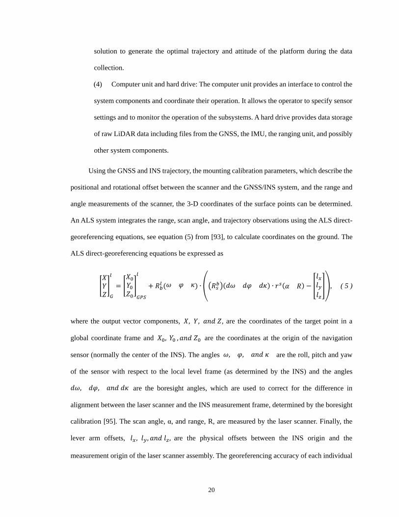
Using the GNSS and INS trajectory, the mounting calibration parameters, which describe the

positional and rotational offset between the scanner and the GNSS/INS system, and the range and

angle measurements of the scanner, the 3-D coordinates of the surface points can be determined.

An ALS system integrates the range, scan angle, and trajectory observations using the ALS direct-

georeferencing equations, see equation (5) from [93], to calculate coordinates on the ground. The

ALS direct-georeferencing equations be expressed as

[𝑋𝑌𝑍]

𝐺

𝑙

= [

𝑋0

𝑌0

𝑍0

]

𝐺𝑃𝑆

𝑙

+ 𝑅𝑏𝑙 (𝜔 𝜑 𝜅) ∙ ((𝑅𝑠

𝑏)(𝑑𝜔 𝑑𝜑 𝑑𝜅) ∙ 𝑟𝑠(𝛼 𝑅) − [

𝑙𝑥𝑙𝑦𝑙𝑧

]), ( 5 )

where the output vector components, 𝑋, 𝑌, 𝑎𝑛𝑑 𝑍, are the coordinates of the target point in a

global coordinate frame and 𝑋0, 𝑌0 , 𝑎𝑛𝑑 𝑍0 are the coordinates at the origin of the navigation

sensor (normally the center of the INS). The angles 𝜔, 𝜑, 𝑎𝑛𝑑 𝜅 are the roll, pitch and yaw

of the sensor with respect to the local level frame (as determined by the INS) and the angles

𝑑𝜔, 𝑑𝜑, 𝑎𝑛𝑑 𝑑𝜅 are the boresight angles, which are used to correct for the difference in

alignment between the laser scanner and the INS measurement frame, determined by the boresight

calibration [95]. The scan angle, α, and range, R, are measured by the laser scanner. Finally, the

lever arm offsets, 𝑙𝑥 , 𝑙𝑦, 𝑎𝑛𝑑 𝑙𝑧, are the physical offsets between the INS origin and the

measurement origin of the laser scanner assembly. The georeferencing accuracy of each individual

21

sample is affected by INS altitude errors, boresight errors, laser scanner errors, lever-arm offset

errors, and GPS positioning errors, as well as the data acquisition parameters (flight height, scan

angle range). A detailed discussion of error analysis for kinematic laser scanning can be found in

previous works [93], [95], [96]. The calibration process ensures that all systematic factors that can

affect the geometrical accuracy of the point cloud are accounted for [93].

Most ALS systems record multiple surface reflections, or “returns,” from a single laser pulse.

When a laser pulse encounters vegetation, power lines, or buildings, multiple returns can be

recorded. The first return will represent the elevation near the top of the object. The second and

third returns may represent trunks and branches within a tree or understory vegetation. Ideally, the

last return recorded by the sensor will be the remaining laser energy reflected off the ground surface;

though at times, dense vegetation can block all of the pulse energy from reaching the ground. These

multiple returns can be used to determine the height of trees or power lines, or to provide

information about forest structure, including but not limited to crown height and understory density.

It has been shown that ALS is an accurate, fast, and versatile 3-D measurement technique

[97] which can complement, or partly replace, other existing geo-data acquisition technologies. As

more ALS collections become available, it will open up exciting new areas of change detection

applications in the Earth Sciences. In fact, ALS data has been employed for a variety of tasks in

this field including biodiversity and ecosystem health monitoring [98], [99], natural resource

management [100]–[102], detection of abrupt catastrophic changes, such as measuring and

quantifying post-earthquake and tsunami damage [49], [55], [69], [103], [104], cumulative land use

change for both urban land cover [105] and deforestation [106], [107], and tectonic fault mapping

[65], [108]–[110]. As the number of repeat ALS datasets increases, new applications for temporally

spaced ALS will continue to emerge as well, motivating this work.

22

2.2 LiDAR Point Cloud

A LiDAR dataset is a collection of points, called a point cloud, and every point in the point

cloud has horizontal coordinates (X and Y) and a vertical elevation (Z). In addition to elevation

values, a point cloud also provides a common format for storing additional information such as

laser intensity, scan angle, return information, etc. Some of this additional information, such as

intensity, can be very useful for visualization. Intensity is how much energy from the laser pulse

was returned to the sensor. There are a lot of factors that affect the amount of energy returned, such

as surface roughness, atmospheric affects, near infrared energy absorption, etc. Therefore, intensity

is typically uncalibrated, so this data is only suitable for a qualitative visual analysis. However,

LiDAR intensity can create a decent black and white “pseudo-image” from the exact time of

LiDAR acquisition, which can be used as supplementary information.

Rasterization of a point cloud is another way of representing the LiDAR data. Range images,

2-D images in regular grid format, are formed when range values (Z) are projected on a regular 2-

D sampling lattice generated from the X and Y coordinates of the point cloud [111]. Thus, they are

conceptually equivalent to regular intensity images, but the intensity attribute is replaced by the

distance from the sensor to the physical location imaged at the corresponding pixel. Because of this

equivalence, range images allow easy, though not always appropriate, substitution of operators

from traditional 2-D image signal processing to the domain of 3-D data processing. After a range

image is generated, objects on the ground like buildings, trees and cars are distinguished by

analyzing the object heights with the DSM. Several researchers have opted to work exclusively

with this representation to perform visual processing tasks [112]. This surface can then be textured

with a digital image, if one is available, creating a 2.5D image called a “texel image” [113]. The

texel image is, therefore, a fused dataset, where the spatial resolution of the image pixels are higher

than the resolution of the LiDAR sensor. However, the sensor geometry of laser range scanners

does not conform to the regular lattice structure of an image. Because of this, the construction of

23

range-images from raw input point clouds can involve some loss of information resulting from the

projection of multiple 3-D points on a single 2-D range image pixel [114]. A related issue occurs

when there is a mismatch between range image resolution and scanner resolution; there may be

cells for which no data points were observed. Traditional image processing operators, such as

convolution filters, are not equipped to handle these “empty” range cells. In addition, for

applications relevant to geomorphology, it is reasonable to expect multiple observations to be made

of the same scene from different vantage points. In this scenario, it is not straightforward to combine

information from multiple range images of the same scene without reverting to the original 3-D

input space.

Point clouds are frequently displayed as surface models or meshes, such as a triangulated

interconnected network (TIN or wireframe model) [115]–[117], which describe the scanned scene

more succinctly than the point clouds themselves. Meshes are undirected graphs composed of a

collection of vertices and edges, whose faces represent discrete piecewise approximations of

surfaces. Unlike range images, meshes have the advantage of allowing irregular surface sampling.

Triangulated meshes have been particularly popular due to a combination of their simple data

format and the fact that modern graphics hardware pipelines support extremely fast rendering of

triangles. Extensive research has gone into the construction of meshes and toward extending signal

processing concepts to them [115], [118], [119]. For example, geomorphological features can be

composed based on meshes and, along with other sources, such as orthorectified air photos and

prior field experience, the geomorphological features can be categorized based on multi-scale

image segmentation using geomorphometrical parameters. These objects can be classified using

setup parameters, such as slope, curvature, and topographic openness, that are measured over

various distances [120][121]. However, meshes are normally not a direct output of a 3-D sensor.

The construction of a mesh from noisy data is not straightforward and requires the removal of noise

and additional pre-processing that can undesirably remove geometric detail. Like range images,

24

meshes are also cumbersome to add information to. For example, the addition of a newly observed

3-D point would require breaking and reconstructing the original mesh.

There are advantages and disadvantages to each type of visualization. Features like bridges

and tree canopies are much better represented in a point cloud than in a TIN. In TIN visualizations,

a bridge tends to form an artificial dam and trees tend to form cones, neither of which reflects reality.

Break lines and spikes, which do not exist in the point cloud, are often introduced during the process

of creating a TIN. However, the gridded two dimensional DSMs, pre- and post-earthquake, can

also reveal spectacular images of fault zone deformation, providing a tantalizing glimpse of the

potential offered by differential LiDAR.

In contrast to the alternatives, working directly with raw point clouds in the input 3-D space

offers several advantages. A point cloud enables 3-D visualization at various scales. It can reveal

the topography setting and large scale geomorphic trends and, at the same time, provide a close up

examination of small scale features, such as centimeter-level topographic undulation, urban

environment rooftop ridges, and even tree leaf area. Point clouds are a natural way to represent 3-

D sensor output and there is no assumption of available connectivity information or underlying

topology. It is also better suited for dynamic applications requiring data addition and deformation.

Another advantage to using a point cloud is that its products require less processing and quality

control, preserving the original positioning and elevation information without introducing

interpolation errors [33].

2.3 Change Detection Using Temporal Spaced LiDAR

While repeat LiDAR documentation over the same location can provide temporally spaced

3-D measurements of targeted topography and land use, it does not directly provide an absolute

model of how the terrain varies spatially. This research explores the issues of change detection

using temporally spaced LiDAR by first presenting current methods used in 3-D point cloud

25

registration and variation detection. Existing methods include 1-D slope-based, 2-D image-based,

DEM/mesh-based, 3-D least-square-based, and probability-based methods. The algorithms for each

will be presented in the following sections.

2.3.1 1-D Slope-Based

A registration method, based on local slope analysis for LiDAR datasets over rough terrain

[68], was proposed using comparison and statistical analysis of local slope versus local elevation

difference between overlapping surfaces to estimate both vertical and horizontal offsets between

the two surfaces.

ΔZ

Xoffset

Zoffset

mx = dz/dz

Z

X

Figure 3 A diagram showing a pair of offset cross sections and the relationship between systematic

horizontal and vertical offset.

A horizontal shift between two flat areas will show no apparent elevation difference; however,

an elevation difference becomes apparent when the two surfaces are sloped. As the slope increases,

the apparent elevation difference grows larger in magnitude. The elevation difference is positive or

negative depending on the local slope, which determines whether a dataset is above or below its

neighbor when shifted.

Figure 3 shows a simple one-dimensional diagram that demonstrates the relationship

between local topographic slope (m𝑥 ), systematic horizontal and vertical offsets of the lines

(x𝑜𝑓𝑓𝑠𝑒𝑡 and z𝑜𝑓𝑓𝑠𝑒𝑡), and the apparent elevation difference (∆z):

26

∆𝑧 = 𝑧𝑜𝑓𝑓𝑠𝑒𝑡 − 𝑥𝑜𝑓𝑓𝑠𝑒𝑡 × 𝑚𝑥 . ( 6 )

The slope-based method of co-registration is often used to improve the relative accuracy of

a LiDAR dataset over rough terrain [68]. Dividing the data into separate flight lines and

recombining them more precisely can improve the relative horizontal accuracy.

2.3.2 2-D Alignment for 3-D Point Clouds

2.3.2.1 Surface Model Differencing

Surface model based change detection provides quantitative measures on a cell-by-cell basis

and also reveals 2-D spatial changes in patterns based on clusters of cells, which may be more

diagnostic than magnitudes of change. Although a DSM may be produced in a variety of data model

forms, the following discussion assumes conventional two-dimensional arrays (cellular or finite-

difference) of orthogonally gridded elevation data. The term ‘DEM’ refers to the square-cell data

model.

The differencing of sequential DEMs to create a DEM of Difference (DoD) or change in the

elevation grid is particularly relevant to geomorphic studies because a DoD can provide a high

resolution, spatially distributed surface model of topographic and volumetric change through time.

This form of geomorphic change detection is a powerful tool that may be used to identify and

quantify spatial patterns of geomorphic change. Once two DEMs have been developed and

registered to the same grid tessellation, a DoD can be made by subtracting the earlier DEM from

the later DEM:

∆𝐸𝑖𝑗 = 𝑍𝑖𝑗2 − 𝑍𝑖𝑗

1, ( 7 )

where ∆Eij is the i, j grid value of the change in elevation model, Zij1 is the i, j value of the earlier

DEM, and Zij2 is the i, j value of the later DEM [122]. The resulting DoD describes reductions in

27

elevation as negative values and increases in elevation as positive values. Determining the cause of

this change (e.g., erosion, deposition, subsidence, anthropogenic modification, precision, accuracy,

or uncertainty) is more challenging, because the required gridding or rasterization of the point

clouds results in information loss. Recent studies that have used DEMs for change detection in

order to map or monitor pre- and post-earthquake fault zone deformation, [8], [54], [120], and [121],

provide a tantalizing glimpse of the potential offered by differential LiDAR. Other sources, such

as orthorectified air photos and prior field measurements, slope, curvature, and topographic

openness [120][121] generated from DEMs, can also be used for DoD related studies.

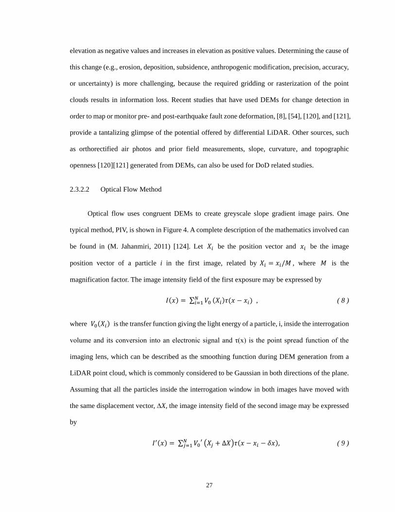
2.3.2.2 Optical Flow Method

Optical flow uses congruent DEMs to create greyscale slope gradient image pairs. One

typical method, PIV, is shown in Figure 4. A complete description of the mathematics involved can

be found in (M. Jahanmiri, 2011) [124]. Let 𝑋𝑖 be the position vector and 𝑥𝑖 be the image

position vector of a particle i in the first image, related by 𝑋𝑖 = 𝑥𝑖/𝑀 , where 𝑀 is the

magnification factor. The image intensity field of the first exposure may be expressed by

𝐼(𝑥) = ∑ 𝑉0𝑁𝑖=1 (𝑋𝑖)𝜏(𝑥 − 𝑥𝑖) , ( 8 )

where 𝑉0(𝑋𝑖) is the transfer function giving the light energy of a particle, i, inside the interrogation

volume and its conversion into an electronic signal and τ(x) is the point spread function of the

imaging lens, which can be described as the smoothing function during DEM generation from a

LiDAR point cloud, which is commonly considered to be Gaussian in both directions of the plane.

Assuming that all the particles inside the interrogation window in both images have moved with

the same displacement vector, ∆X, the image intensity field of the second image may be expressed

by

𝐼′(𝑥) = ∑ 𝑉0′𝑁

𝑗=1 (𝑋𝑗 + ∆𝑋)𝜏(𝑥 − 𝑥𝑖 − 𝛿𝑥), ( 9 )

28

where 𝛿𝑥 is the particle image displacement, which can reasonably be approximated by ∆𝑋 ≅

𝛿𝑥/𝑀.

Figure 4 An illustration of PIV (a flow vector method), using the cross-correlation of a pair of two

singly collected images.

The cross-correlation of the two interrogation windows is defined as

𝑅(𝑠) = [𝐼(𝑥)𝐼(𝑥 + 𝑠)], ( 10 )

where s is the separation vector in the correlation plane and I is the spatial averaging operator over

the interrogation window. R can be decomposed into three parts

𝑅(𝑠) = 𝑅𝐶(𝑠) + 𝑅𝐹(𝑠) + 𝑅𝐷(𝑠), ( 11 )

where 𝑅𝐶 is the correlation of the mean image intensities and 𝑅𝐹 is the fluctuating noise

component, both resulting from the i ≠ j terms. The displacement-correlation peak, 𝑅𝐷, represents

the component of the cross-correlation function corresponding to the correlation of particles from

the first image with identical particles present in the second image (i = j terms). This peak reaches

a maximum for s = 𝛿𝑥. Therefore, the determination of the location of this maximum yields ∆X.

This location is commonly obtained through systematic exploration in the interrogation window by

using Fast-Fourier Transform algorithms for computing cross-correlation. In the general case when

all particles inside the interrogation window do not have uniform velocities, due to turbulence or

velocity gradients, the location of the maximum yields the most probable displacement within the

Time 𝜏

Time 𝜏 + ∆𝑡

Velocity vector

29

interrogation window. The value of s is determined with sub-pixel accuracy from correlation data

interpolation, obtained through a fit of these data to some modelling function, e.g., a Gaussian

profile.

In order to maximize the effectiveness of PIV, a smoothing function is applied to minimize

the differences in texture between the multi-temporal datasets. This is accomplished using a low-

pass filter that calculates mean values to reduce the extreme values within each dataset. PIV applies

a direct cross-correlation algorithm to find correspondence between the two images. The algorithm

is computationally complex; it incorporates signal processing of the phase shifts via Fast Fourier

Transform (FFT) and applies a Gaussian fit function to find the correlation peak.

In topographic change detection, the application of PIV is based on two primary variables,

the interrogation area and the step spacing (i.e., resolution). The interrogation area represents the

extent to which the application will search for the corresponding pixel values and, therefore, must

be greater than the maximum expected displacement. The PIVlab program [125] incorporates an

iterative multistep process with decreasing interrogation areas and increasing resolution. The initial

run produces an imprecise but relatively smooth displacement field; subsequent runs deform the

images based on the initial results to refine the process and improve the correlation peak. PIV was

applied to sequential LiDAR datasets to measure surface displacement on actively deforming

landscapes, such as landslide geodesy [126] and ground deformation caused by earthquakes in

Japan [69].

2.3.3 3-D Registration-Closest Point Criterion (CPC) Based

If point correspondences between the two point clouds are available, an intuitive 3-D

registration approach would be to directly minimize the sum of the Euclidean distances between

these points. This corresponds to a linear least-squares problem that can be solved robustly using

the SVD method [127]. The SVD algorithm directly solves the least-squares problem, thereby

30

assuming perfect data. If point correspondences are not available, point correspondences between

the point clouds can be defined based on the closest point criterion (CPC). Besl and McKay [72]

introduced a method that iteratively disregards outliers in order to improve upon the previous

estimate of registration parameters. Their method, Iterative Closest Point (ICP), is illustrated

conceptually in Figure 5; the algorithm is described in more detail in the next sections.

Figure 5 ICP overview scheme.

2.3.3.1 Standard Iterative Closest Point (ICP)

Iterative Closest Point (ICP) is an algorithm that iteratively matches two point sets, a source

point cloud and a target point cloud, which for convenience we shall denote by P and Q in R𝑑, with

their elements being denoted by {p𝑖}, 𝑖 = 1…𝑁𝑝 𝑎𝑛𝑑 {q𝑖}, 𝑖 = 1…𝑁𝑞. We are interested in a

point to point matching function, 𝑓, that matches P and Q, i.e., 𝑓(p𝑖), corresponds to q𝑖, and that

minimizes the root mean squared distance (RMSD) between P and Q. Mathematically, we want to

minimize the following

𝑅𝑀𝑆𝐷(𝑃, 𝑄, 𝑓) = √1

𝑛∑ ‖𝑝𝑖 − 𝑓(𝑝𝑖)‖

2𝑝𝑖∈𝑃 . ( 12 )

Thus a rigid transformation, a combination of rotation matrix R, translation vector t, and

possibly scale S, can be estimated to minimize the sum of the RMSD (error).

𝑚𝑖𝑛𝑅, 𝑡

𝑅𝑀𝑆𝐷 (𝑅𝑃 − 𝑡, 𝑄, 𝑓) = 𝑚𝑖𝑛𝑓:𝑃→𝑄, 𝑡∈𝑅𝑑, 𝑅∈𝑆𝑂(𝑑)

∑ ‖𝑅𝑝𝑖 − 𝑡 − 𝑓(𝑝𝑖)‖2

𝑝𝑖⃗⃗ ⃗∈𝑃 , ( 13 )

where 𝑆𝑂(𝑑) is a set of special orthogonal matrices in d dimensions. Each iteration of the

correspondence incorporates a matching step and a transformation step. Steps 1, 2, and 3 below are

Source

Target

Correspondences SVD Transform Output

Iteration

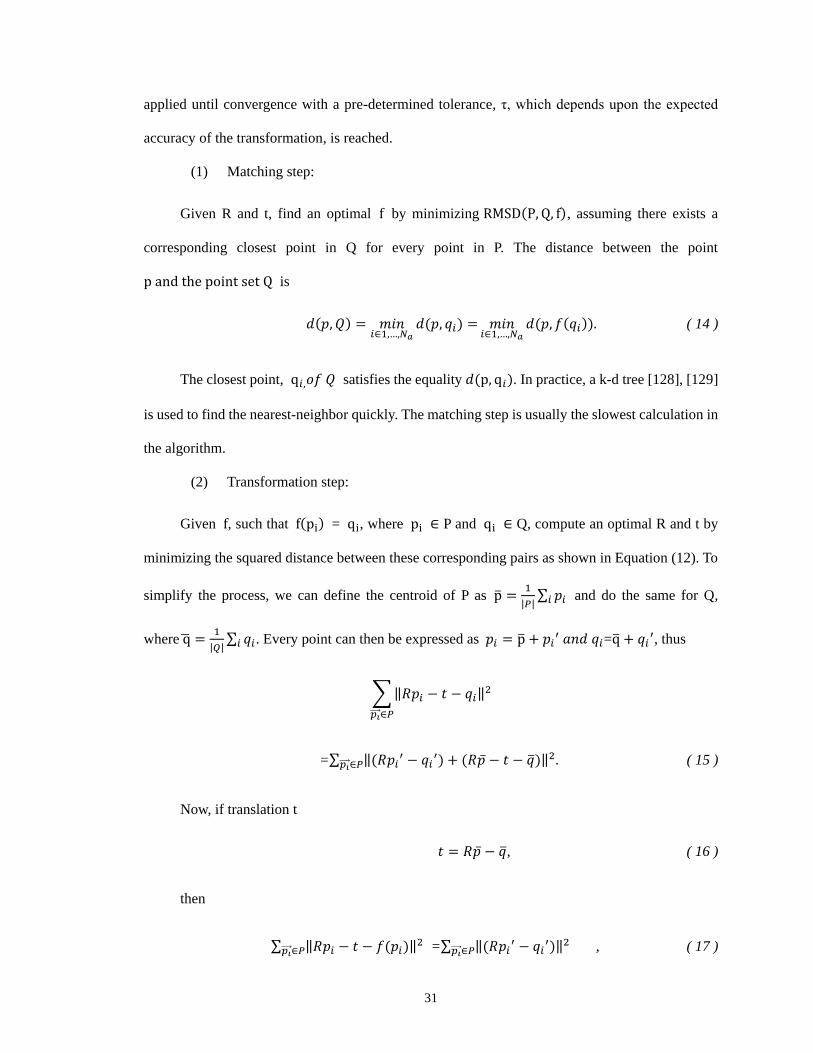
31

applied until convergence with a pre-determined tolerance, τ, which depends upon the expected

accuracy of the transformation, is reached.

(1) Matching step:

Given R and t, find an optimal f by minimizing RMSD(P, Q, f), assuming there exists a

corresponding closest point in Q for every point in P. The distance between the point

p and the point set Q is

𝑑(𝑝, 𝑄) = 𝑚𝑖𝑛𝑖∈1,…,𝑁𝑎

𝑑(𝑝, 𝑞𝑖) = 𝑚𝑖𝑛𝑖∈1,…,𝑁𝑎

𝑑(𝑝, 𝑓(𝑞𝑖)). ( 14 )

The closest point, q𝑖,𝑜𝑓 𝑄 satisfies the equality 𝑑(p, q𝑖). In practice, a k-d tree [128], [129]

is used to find the nearest-neighbor quickly. The matching step is usually the slowest calculation in

the algorithm.

(2) Transformation step:

Given f, such that f(pi) = qi, where pi ∈ P and qi ∈ Q, compute an optimal R and t by

minimizing the squared distance between these corresponding pairs as shown in Equation (12). To

simplify the process, we can define the centroid of P as p̅ =1

|𝑃|∑ 𝑝𝑖𝑖 and do the same for Q,

where q̅ =1

|𝑄|∑ 𝑞𝑖𝑖 . Every point can then be expressed as 𝑝𝑖 = p̅ + 𝑝𝑖

′ 𝑎𝑛𝑑 𝑞𝑖=q̅ + 𝑞𝑖′, thus

∑‖𝑅𝑝𝑖 − 𝑡 − 𝑞𝑖‖2

𝑝𝑖⃗⃗ ⃗∈𝑃

=∑ ‖(𝑅𝑝𝑖′ − 𝑞𝑖

′) + (𝑅�̅� − 𝑡 − �̅�)‖2.𝑝𝑖⃗⃗ ⃗∈𝑃 ( 15 )

Now, if translation t

𝑡 = 𝑅�̅� − �̅�, ( 16 )

then

∑ ‖𝑅𝑝𝑖 − 𝑡 − 𝑓(𝑝𝑖)‖2

𝑝𝑖⃗⃗ ⃗∈𝑃 =∑ ‖(𝑅𝑝𝑖′ − 𝑞𝑖

′)‖2𝑝𝑖⃗⃗ ⃗∈𝑃 , ( 17 )

32

so that

∑‖(𝑅𝑝𝑖′ − 𝑞𝑖

′)‖2

𝑝𝑖⃗⃗ ⃗∈𝑃

= 𝑅𝑅𝑇 ∑‖𝑝𝑖′‖2 − 2𝑡𝑟 (𝑅 ∑𝑝𝑖

′𝑞𝑖′𝑇

𝑛

𝑖=1

) + ∑‖𝑞𝑖′‖2

𝑛

𝑖=1

𝑛

𝑖=1

= ∑ ‖𝑝𝑖′‖2 − 2𝑡𝑟(𝑅 ∑ 𝑝𝑖

′𝑞𝑖′𝑇𝑛

𝑖=1 ) + ∑ ‖𝑞𝑖′‖2.𝑛

𝑖=1𝑛𝑖=1 ( 18 )

Because R is an orthogonal matrix, we have

𝑅𝑅𝑇 = 𝐼. ( 19 )

Let N=∑ 𝑝𝑖′𝑞𝑖

′𝑇𝑛𝑖=1 , so that the problem of minimizing RMSD becomes maximizing

𝑡𝑟(𝑅𝑁). ( 20 )

The optimal rotation, 𝑅, can be calculated using a singular value decomposition (SVD) of

the matrix N=U∑V𝑇, where U and V are orthogonal matrices, the diagonals of Σ are the singular

values of 𝑁, and

Σ= diag (𝜎1, 𝜎2,… 𝜎𝑑) , 𝜎1 ≥𝜎2 ≥ ... ≥𝜎𝑑 ≥ 0. ( 21 )

It is shown in [130] that to minimize equation (6) the rotation matrix should be defined as

R =VUT. ( 22 )

(3) Return to step 2:

Terminate the iteration when the change in 𝑅𝑀𝑆𝐷 falls below a preset threshold, τ>0,

specifying the desired precision of registration, 𝑑𝑘 − 𝑑𝑘+1 < 𝜏.

By iteratively applying this minimization, an optimal result that is, if not a global minima, a

local minima near the global minima, can be guaranteed. During each iteration, the transformation

33

step uses least squares registration to reduce the average distance between corresponding points,

whereas the matching step finds a new corresponding pair by using the closest point determination.

As a result, the sum of square error is a monotonically decreasing function with respect to the

number of iterations. For a complete proof the reader is referred to Besl and McKay (1992) [25].

To date, the primary method for determining 3-D transformation between LiDAR point

clouds is through the use of the iterative closest point (ICP) algorithm and its variants [74]. This

approach is efficient and easy to implement but it depends heavily on initialization and often

converges to the local minimum as a result of noise, outliers, limited amount of overlap, and low

data resolution of either point cloud.

2.3.3.2 Piecewise Rigid Transformation

In some applications the target data cannot be considered as a cohesive whole entity or it

may have a spatially varying displacement. In these cases, it is common to first segment the data

into smaller tiles that are suitable for rigid transformation. This is especially true for large scale

topographic geomorphology, such as earthquake movement and fault slip shift determination

[49][7]. Typically, displacement values are estimated within an area covered by a window of fixed

length [7]. Pre-defining the size of tiles that compose the entire dataset can be critical. There is

always a trade-off between calculation efficiency, convergence speed, extent of detection detail,

and complexity when using these types of detection methods. However, the use of a fixed length

window for change detection of spatially varying parameters may be problematic and lead to

incorrect analyses, either by delaying the detection of change or not detecting the change in the first

place.

To mitigate this problem, a moving window solution can be borrowed from image processing

[131]–[135] to significantly improve singularity detection without compromising a robust

investigation of all candidate points. Searching in a finite set of plausible clusters instead of a fixed

34

shape tile is another potential alternative to the moving window technique. In image processing,

the moving window process involves passing a window (e.g., a square 9 pixel window) over the

image pixel-by-pixel. It returns a value for the central pixel that takes into account all of the pixel-

values covered by the window. Similarly, for a point cloud, the window is moved in 3-D space. For

example, the window is moved horizontally on the x-y plane, creating the shape of a cuboid, and

points that fall into the space within each window will be considered for the respective calculation.

The simplest algorithms return statistics, such as the average or mode value, that are used to both

detail and smooth the registration results. These derived results can often reveal much more useful

information regarding the change detection of surface features. The specifics of the moving window

process, including a given window shape, window size, and stepping size, are decided on a case by

case basis. The moving window allows a higher density estimation of the change at the scale of the

fractional step size instead of the tile size but it also acts as a low pass filter, smoothing local

discontinuities that may be present in the ICP solution due to factors such as spurious data or ICP

algorithm convergence problems [64].

2.3.3.3 Optimization of ICP

A. Selection of Points

Standard ICP always uses all available points, however, as a result, the computational cost

can be high when a large number of points are selected for minimization. There are several

subsampling methods that preselect which points are passed to future iterations, based on the

assumption that the point cloud always has a redundant number of points for registration. Common

sampling methods are:

1) Uniform subsampling of the available points. [136]

2) Random sampling (with a different sample of points at each iteration). [137]

3) Normal-space sampling.

35

Commonly adopted uniform subsampling takes proportional samples from the point cloud.

For example, it might sample 1 point/m2, regardless of the local surface geometry; thus the

difference in sampling biases the error term towards fitting larger regions better than smaller ones

and sometimes does not constrain the transformation fully. A strategy such as random sampling

will often select only a few samples within the primary features, leading to an inability to determine

certain components of the correct rigid-body transformation. Normal-space sampling segments the

points according to the position of the normals in angular space and then samples as uniformly as

possible across the segments [138]. It is a very simple example of using surface features for

alignment; it has lower computational cost, but lower robustness, than traditional feature-based

methods. The performance of uniform subsampling, random sampling, and normal-space sampling

is compared to convergence performance in [74]. The result indicates that, for a scene with a good

distribution of normals, the exact sampling strategy is not critical. But for a case with small local

or sudden changes, only the normal-space sampling is able to converge.

B. Matching Points

For each sampled point cloud, the next stage of ICP is the correspondence finding algorithm

(i.e., point matching):

1) Find the closest point in the other mesh. This computation may be accelerated using

a k-d tree and/or closest point caching. [139]

2) “Normal shooting.” Find the intersection of the ray originating at the source point in

the direction of the source point’s normal with the destination surface. [140].

3) “Reverse calibration.” Project the source point onto the destination mesh, from the

point of view (POV) of the destination mesh’s range camera [141], and then perform a

search in the destination range image.

Although the “Reverse calibration” algorithm is faster than closest point finding or normal

shooting, even when involving a closest-point search accelerated with a k-d tree, because it is

36

performed at a constant rate for each iteration, rather than involving a closest-point search, it is not

a preferred method because the ranging mechanism (i.e., camera POV) of each point cloud is not

always available.

C. Error Metric and Minimization

Finally, we need to define a criteria for iterative convergence. The following error metrics

have been used in previous work:

1) Sum of squared distances between corresponding points, i.e., the “point to point”

metric. For an error metric of this form, there exists, a closed form solution for determining

the rigid-body transformation that minimizes the error.

2) The “compatible point to point” metric, which takes into account both the distance

between points and the compatibility of intensity or color, and restricts the solution to only

matching points compatible with the source point according to a given metric [142].

3) Sum of squared distances from each source point to the plane containing the

destination point and oriented perpendicular to the destination normal [140]. In this “point

to plane” case, no closed-form solutions are available.

The least-squares equations for the “point to plane” method may be solved using a generic

nonlinear approach (e.g., Levenberg-Marquardt) or by simply linearizing the equations. In practice,

the linear approximation method can be used even when the relative orientation between the two

input surfaces is quite large, sometimes as large as 30°, which is described in [143]. However, this

is very dependent on the geometry and the amount of overlap between the two input surfaces. As

the relative orientation decreases after each ICP iteration, the linear approximation becomes more

accurate. To improve the numerical stability of the computation, it is important to use a unit of

distance that is comparable in magnitude with the rotation angles.

37

D. Multi Scale / resolution ICP (Multi-res ICP).

Algorithms that switch between variants of ICP, depending on the local error landscape and

the probable presence of local minima, might also provide increased robustness. Therefore, by

making the first few iterations using down sampled data and then increasing the resolution of the

data in the following iterations, multiresolution ICP can create a coarse to fine matching strategy.

The main expected advantage of multiresolution ICP is the reduction of the computational cost,

given that the duration of each iteration is reduced at lower resolutions. The precision of the final

match is expected to be the same as that using monoresolution ICP, with all the points for the whole

registration. In addition, we expect the total number of iterations to be smaller than in the

“monoresolution” case.

E. Weighting of pairs

The final piece of the ICP algorithm that we will examine is the effect of assigning different

weights to the corresponding point pairs found in the previous steps. The standard ICP procedure

implicitly assumes that the input point sets are subject to isotropic zero-mean Gaussian noise, which,

for ALS, is generally an incorrect assumption. In addition to differing weights for each point, the

horizontal uncertainty can be 2 to 5 times larger than the vertical uncertainty for an ALS solution

[93]. Therefore, based on the original Besl and McKay (1992) formulation, several ICP variants

have been proposed which include additional properties such as color [27], invariant geometric

features [28], inter-point distance [29], and the compatibility of normal, or surface normal, [26] in

the distance metric. In a review paper, Rusinkiewicz and Levoy [43] classified the proposed

variants of the ICP algorithm into six subtasks: selection, matching, weighting, outlier removal,

error metric, and minimization. However, their comparisons of variants focused largely on the

speed of algorithm convergence instead of the stability, robustness, and correctness of the derived

rigid body transformation [74][147][138]. In fact the likelihood of anisotropic localization errors

has so far been given very little attention [148], with other research assuming that all points in the

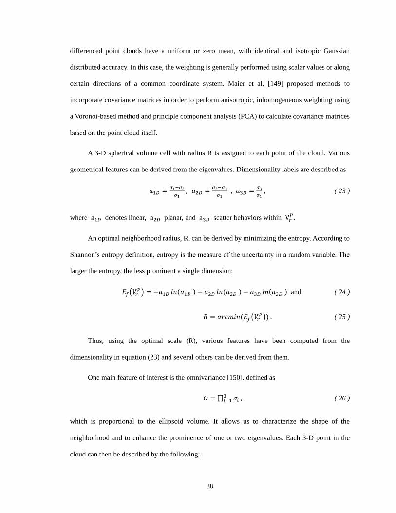
38

differenced point clouds have a uniform or zero mean, with identical and isotropic Gaussian

distributed accuracy. In this case, the weighting is generally performed using scalar values or along

certain directions of a common coordinate system. Maier et al. [149] proposed methods to

incorporate covariance matrices in order to perform anisotropic, inhomogeneous weighting using

a Voronoi-based method and principle component analysis (PCA) to calculate covariance matrices

based on the point cloud itself.

A 3-D spherical volume cell with radius R is assigned to each point of the cloud. Various

geometrical features can be derived from the eigenvalues. Dimensionality labels are described as

𝑎1𝐷 =𝜎1−𝜎2

𝜎1, 𝑎2𝐷 =

𝜎2−𝜎3

𝜎1 , 𝑎3𝐷 =

𝜎3

𝜎1 , ( 23 )

where a1𝐷 denotes linear, a2𝐷 planar, and a3𝐷 scatter behaviors within V𝑟𝑝

.

An optimal neighborhood radius, R, can be derived by minimizing the entropy. According to

Shannon’s entropy definition, entropy is the measure of the uncertainty in a random variable. The

larger the entropy, the less prominent a single dimension:

𝐸𝑓(𝑉𝑟𝑝) = −𝑎1𝐷 𝑙𝑛(𝑎1𝐷 ) − 𝑎2𝐷 𝑙𝑛(𝑎2𝐷 ) − 𝑎3𝐷 𝑙𝑛(𝑎3𝐷 ) and ( 24 )

𝑅 = 𝑎𝑟𝑐𝑚𝑖𝑛(𝐸𝑓(𝑉𝑟𝑝)) . ( 25 )

Thus, using the optimal scale (R), various features have been computed from the

dimensionality in equation (23) and several others can be derived from them.

One main feature of interest is the omnivariance [150], defined as

𝑂 = ∏ 𝜎𝑖3𝑖=1 , ( 26 )

which is proportional to the ellipsoid volume. It allows us to characterize the shape of the

neighborhood and to enhance the prominence of one or two eigenvalues. Each 3-D point in the

cloud can then be described by the following:

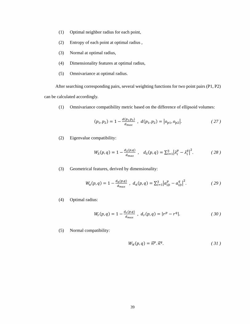
39

(1) Optimal neighbor radius for each point,

(2) Entropy of each point at optimal radius ,

(3) Normal at optimal radius,

(4) Dimensionality features at optimal radius,

(5) Omnivariance at optimal radius.

After searching corresponding pairs, several weighting functions for two point pairs (P1, P2)

can be calculated accordingly.

(1) Omnivariance compatibility metric based on the difference of ellipsoid volumes:

(𝑝1, 𝑝2) = 1 −𝑑(𝑝1,𝑝2)

𝑑𝑚𝑎𝑥 , 𝑑(𝑝1, 𝑝2) = |𝑜𝑝1, 𝑜𝑝2|. ( 27 )

(2) Eigenvalue compatibility:

𝑊𝜆(𝑝, 𝑞) = 1 −𝑑𝜆(𝑝,𝑞)

𝑑𝑚𝑎𝑥 , 𝑑𝜆(𝑝, 𝑞) = ∑ |𝜆𝑖

𝑝− 𝜆𝑖

𝑞|23

𝑖=1 . ( 28 )

(3) Geometrical features, derived by dimensionality:

𝑊𝑎(𝑝, 𝑞) = 1 −𝑑𝑎(𝑝,𝑞)

𝑑𝑚𝑎𝑥 , 𝑑𝑎(𝑝, 𝑞) = ∑ |𝑎𝑖𝐷

𝑝− 𝑎𝑖𝐷

𝑞|23

𝑖=1 . ( 29 )

(4) Optimal radius:

𝑊𝑟(𝑝, 𝑞) = 1 −𝑑𝑟(𝑝,𝑞)

𝑑𝑚𝑎𝑥 , 𝑑𝑟(𝑝, 𝑞) = |𝑟𝑝 − 𝑟𝑞|. ( 30 )

(5) Normal compatibility:

𝑊𝑁(𝑝, 𝑞) = �⃗� 𝑝. �⃗� 𝑞. ( 31 )

40

2.3.3.4 Proposed Point Accuracy Estimation - Anisotropic Iterative Closest Point (A-ICP)

As previously mentioned, standard ICP and most of its variants implicitly assume that the

input point sets are subject to isotropic zero-mean Gaussian noise, which is not realistic. Herein,

we review an algorithm that can manage anisotropic localization errors. Anisotropic Iterative

Closest Point (A-ICP) [149] assumes that the principal components of the localization error in each

point, p, are independent and normally distributed with zero mean and a covariance matrix

described by

∑𝑝 = 𝑉𝑃𝑆𝑃2𝑉𝑃

′, ( 32 )

where the columns of 𝑉𝑃 are the principal axes of the localization error and 𝑆𝑃2 is a diagonal

matrix with 𝑆𝑃 = 𝑑𝑖𝑎𝑔(𝜎1, , … , 𝜎𝑑 , ) , where 𝜎𝑖 represents the standard deviation along the

principal axis i. The two-space cross covariance of the localization error is determined as

∑𝑝𝑞 = ∑𝑝 + ∑𝑞. ( 33 )

The anisotropically weighted distance between point p and q can then be defined as the

weighted Euclidean distance

𝑑𝑛𝑒𝑤(𝑝, 𝑞) = ‖𝑊𝑝𝑞(𝑝 − 𝑞)‖2

, ( 34 )

with the weighting matrix given as

𝑊𝑝𝑞 = ∑𝑝𝑞−1/2

. ( 35 )

The A-ICP method iteratively minimizes the anisotropic weighted fiducial registration error

(FRE), given by

𝐹𝑅𝐸𝑤𝑒𝑖𝑔ℎ𝑡𝑒𝑑2 = ∑ ‖𝑊𝑖(𝑅𝑝𝑖 − 𝑡 − 𝑞𝑖)‖2

2𝑁𝑖=1 , ( 36 )

instead of the RMSD.

41

It can be shown that, if the covariance matrices are set to the identity matrix I for all points

and W𝑝𝑞 is set to the weighted FRE (𝐹𝑅𝐸𝑤𝑒𝑖𝑔ℎ𝑡𝑒𝑑), then 𝐹𝑅𝐸𝑤𝑒𝑖𝑔ℎ𝑡𝑒𝑑 is identical to the RMS

distance between corresponding points and thus to the FRE of the original ICP algorithm.

A schematic illustration of the computation of a rigid transformation based on a set of

corresponding points in meshes A and B with (a) the original ICP and (b) the proposed A-ICP is

given in Figure 6. For a better illustration, a 2-D representation was chosen. In Figure 6 (a), a

considerable mis-registration occurs because two of the matched vertices (central vertices) do not

correspond to the same physical position. In Figure 6 (b), we compensate for this effect by setting

the point localization accuracy based on the area of influence of a vertex (represented by the

dimensions of the ellipsoids drawn in that direction), which leads to a decrease in the total error. A-

ICP assumes that the principal components of the localization error in each point are independent

and normally distributed with zero means and anisotropic variance.

(a) ICP (b) (A-ICP)

Figure 6 2-D Schematic illustration of (a) the original ICP and (b) the A-ICP, after [149].

Another important property of A-ICP is that it can be guaranteed to terminate at a global

minimum after a finite number of iterations [149]. The issue of mis-registration can be considerably

mitigated because points with better quality, judged by the point accuracy estimation, are more

highly weighted.

Target

VerticesData A

Data B

Data A

Data B

Target

Vertices

42

2.3.3.5 Choices of Priors and Regulations

We have introduced several ICP variants, next we will choose effective variants for this

research and compare the performance of each in several cases to test the robustness of different

densities, varying geometric features, and different levels of noise for both synthetic and real

earthquake surface deformation data. Based on the discussion above, for the test cases without color

or intensity information, we will choose uniform sampling, use KD-tree acceleration for a fair

comparison, and focus on evaluating the performance of standard ICP, point to plane ICP, and

multiresolution ICP with other 3-D registration methods based on probability (introduced in the

next section).

2.3.4 3-D Registration - Probability-Based

ICP is a typical “hard” assignment method, which assumes that the closest points provide an

estimate of the correct correspondence, an assumption that is often not valid, thus making ICP

sensitive to the initial alignment. Soft assignment is an effort to overcome such limitations. Instead

of looking for "hard" correspondences between points, where each point in one set has to map

uniquely to another point in the other set, "soft" correspondences allow for each point in one of the

sets to correspond to every point in the other set by a weight criteria. For soft assignment, we put

each point in the source point dataset into bins with the number of the points in the target point set,

in proportion to the weight. This avoids a point-wise deterministic correspondence search. Soft

assignment is used in probability-based registration. With a certain probability model, an expected

likelihood is employed to compute the affinity between two distributions, which corresponds to the

similarity between the two point clouds. The most common assumption for probability distribution

is the Gaussian Mixed model (GMM).

43

2.3.4.1 GMM Model

The alignment of two point sets is considered to be a probability density estimation problem,

where one point set represents the Gaussian mixture model (GMM) centroids and the other one

represents the data points [151].

If we consider the point XN×D = (X1 , X2, … , XN)𝑇 is the first point set (the data points),

YM×D = (Y1 , Y2, … , YM)𝑇 is the second point set (the GMM centroids), and the points in X are

generated by the GMM, then the probability density function of data points X is

𝑝(𝑥) = ∑ 𝑃(𝑦𝑚)𝑝 (𝑥

𝑦𝑚)𝑀+1

𝑚=1 , ( 37 )

where 𝑃(𝑦𝑚) is a prior probability of 𝑦𝑚 and

𝑝 (𝑥

𝑦𝑚) =

1

(2𝜋𝜎2)𝐷2

𝑒𝑥𝑝 (−‖𝑥−𝑦𝑚‖2

2𝜎2) ( 38 )

is the density of x given the occurrence of the value 𝑦𝑚, where D is dimension of the point sets

and 𝜎2 is the standard deviation for the conditional probability of the Gaussian model.

If we consider 𝑇(𝑌, 𝜃) as the transformation T applied to Y, where 𝜃 is a set of the

transformation parameters, then to estimate θ, for which the point locations of Y are parameterized

(Y(𝜃) ), as well as 𝜎2, the correspondence probability which is defined as the likelihood of the

GMM centroid (𝑦𝑚) given the data point (𝑥𝑛) must be maximized.

(𝜃, 𝜎2̂) = 𝑎𝑟𝑔 𝑚𝑎𝑥𝜃,𝜎2

(∏ ∑ 𝑃(𝑦𝑚)𝑝 (𝑥𝑛

𝑦𝑚)𝑀+1

𝑚=1𝑁+1𝑛=1 ) , ( 39 )

which equates to minimizing the negative of the logarithm of the objective function

(𝜃, 𝜎2̂) = 𝑎𝑟𝑔 𝑚𝑖𝑛𝜃,𝜎2

(−∑ 𝑙𝑜𝑔 (∑ 𝑃(𝑦𝑚)𝑝(𝑥𝑛/𝑦𝑚))𝑀+1𝑚=1

𝑁+1𝑛=1 ) . ( 40 )

44

2.3.4.2 Optimization Methods

In [152], the authors summarize optimization methods for 3-D registration into three major

categories:

(1) local deterministic optimization: including gradient descent [153], versions of

Gauss-Newton methods, and Expectation Maximization (EM) [154], [155];

(2) global deterministic methods: usually applied with rigid-registration, such as branch

and bound [156], [157] and tree search [139], graduated assignment [158], mean field

annealing [158], game theory framework [159], and spectral correspondence [160].

(3) stochastic optimization: genetic algorithm and simulated annealing, particle filtering,

Hough transform, RANSAC, and Message Passing and Belief Propagation (MRF).

Based on the Gaussian mixture model representation discussed in the last section, an intuitive

reformulation of the point set registration problem is to solve an optimization problem such that a

certain dissimilarity measure between the Gaussian mixtures constructed from the transformed

model set and the fixed scene set is minimized. Here, we chose the Euclidean distance for

measuring the similarity between two Gaussian mixtures for the following two reasons. First, it is

a good comparison because the CPC method uses a similar similarity measurement. Second, there

exists a closed-form expression for the Euclidean distance between Gaussian mixtures, which in

turn affords an efficient implementation of the registration algorithm. To maximize the log-

likelihood, the EM method is used.

2.3.4.3 EM for GMM Frame Work:

At the optimum, two point sets become aligned and the correspondence is obtained using the

maximum of the GMM posterior probability for a given data point [161], [162]. EM minimizes the

expectation of the complete negative log-likelihood function so that:

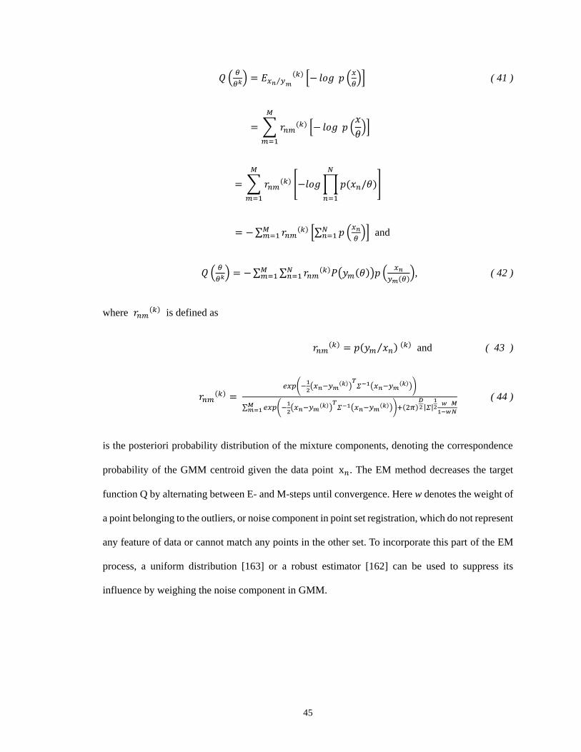
45

𝑄 (𝜃

𝜃𝑘) = 𝐸𝑥𝑛 𝑦⁄𝑚

(𝑘) [− 𝑙𝑜𝑔 𝑝 (𝑥

𝜃)] ( 41 )

= ∑ 𝑟𝑛𝑚(𝑘)

𝑀

𝑚=1

[− 𝑙𝑜𝑔 𝑝 (𝑥

𝜃)]

= ∑ 𝑟𝑛𝑚(𝑘)

𝑀

𝑚=1

[−𝑙𝑜𝑔 ∏𝑝(𝑥𝑛/𝜃)

𝑁

𝑛=1

]

= −∑ 𝑟𝑛𝑚(𝑘)𝑀

𝑚=1 [∑ 𝑝 (𝑥𝑛

𝜃)𝑁

𝑛=1 ] and

𝑄 (𝜃

𝜃𝑘) = −∑ ∑ 𝑟𝑛𝑚

(𝑘)𝑃(𝑦𝑚(𝜃))𝑝 (𝑥𝑛

𝑦𝑚(𝜃))𝑁

𝑛=1𝑀𝑚=1 , ( 42 )

where 𝑟𝑛𝑚(𝑘) is defined as

𝑟𝑛𝑚(𝑘) = 𝑝(𝑦𝑚 𝑥𝑛⁄ ) (𝑘) and ( 43 )

𝑟𝑛𝑚(𝑘) =

𝑒𝑥𝑝(−1

2(𝑥𝑛−𝑦𝑚

(𝑘))𝑇𝛴−1(𝑥𝑛−𝑦𝑚

(𝑘)))

∑ 𝑒𝑥𝑝(−1

2(𝑥𝑛−𝑦𝑚

(𝑘))𝑇𝛴−1(𝑥𝑛−𝑦𝑚

(𝑘)))+(2𝜋)𝐷2 |𝛴|

12

𝑤

1−𝑤𝑀𝑚=1

𝑀

𝑁

( 44 )

is the posteriori probability distribution of the mixture components, denoting the correspondence

probability of the GMM centroid given the data point x𝑛. The EM method decreases the target

function Q by alternating between E- and M-steps until convergence. Here w denotes the weight of

a point belonging to the outliers, or noise component in point set registration, which do not represent

any feature of data or cannot match any points in the other set. To incorporate this part of the EM

process, a uniform distribution [163] or a robust estimator [162] can be used to suppress its

influence by weighing the noise component in GMM.

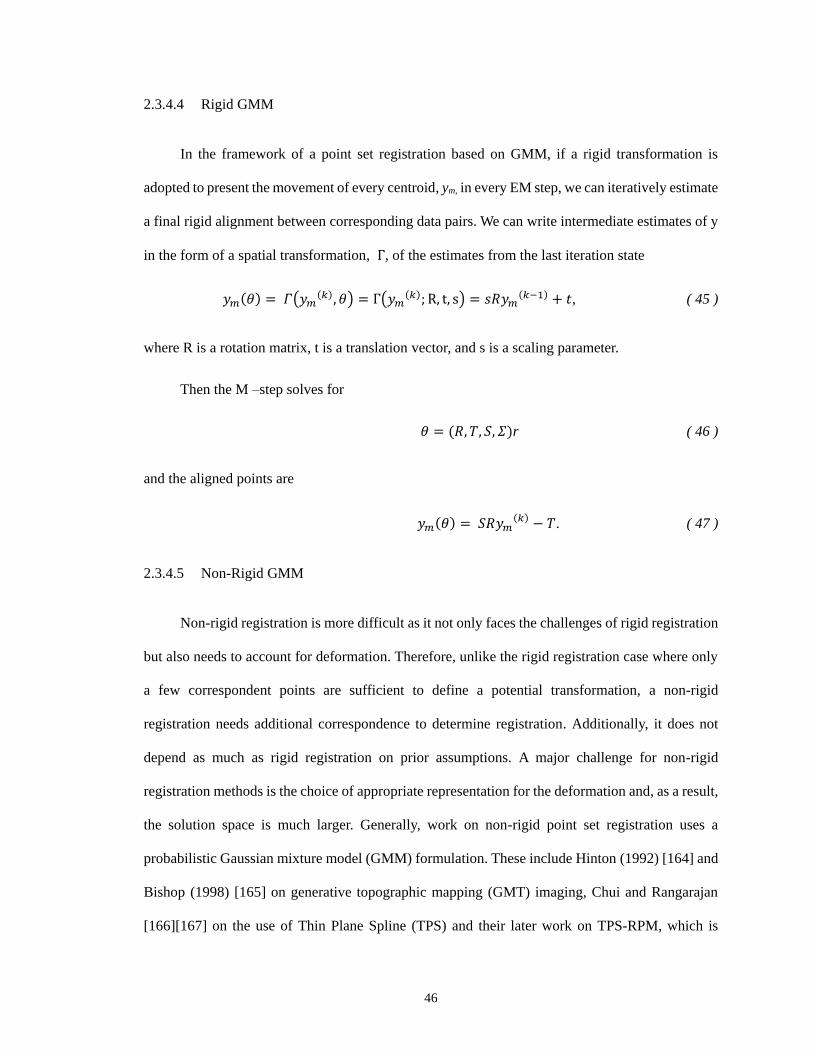
46

2.3.4.4 Rigid GMM

In the framework of a point set registration based on GMM, if a rigid transformation is

adopted to present the movement of every centroid, ym, in every EM step, we can iteratively estimate

a final rigid alignment between corresponding data pairs. We can write intermediate estimates of y

in the form of a spatial transformation, Γ, of the estimates from the last iteration state

𝑦𝑚(𝜃) = 𝛤(𝑦𝑚(𝑘), 𝜃) = Γ(𝑦𝑚

(𝑘); R, t, s) = 𝑠𝑅𝑦𝑚(𝑘−1) + 𝑡, ( 45 )

where R is a rotation matrix, t is a translation vector, and s is a scaling parameter.

Then the M –step solves for

𝜃 = (𝑅, 𝑇, 𝑆, 𝛴)r ( 46 )

and the aligned points are

𝑦𝑚(𝜃) = 𝑆𝑅𝑦𝑚(𝑘) − 𝑇. ( 47 )

2.3.4.5 Non-Rigid GMM

Non-rigid registration is more difficult as it not only faces the challenges of rigid registration

but also needs to account for deformation. Therefore, unlike the rigid registration case where only

a few correspondent points are sufficient to define a potential transformation, a non-rigid

registration needs additional correspondence to determine registration. Additionally, it does not

depend as much as rigid registration on prior assumptions. A major challenge for non-rigid

registration methods is the choice of appropriate representation for the deformation and, as a result,

the solution space is much larger. Generally, work on non-rigid point set registration uses a

probabilistic Gaussian mixture model (GMM) formulation. These include Hinton (1992) [164] and

Bishop (1998) [165] on generative topographic mapping (GMT) imaging, Chui and Rangarajan

[166][167] on the use of Thin Plane Spline (TPS) and their later work on TPS-RPM, which is

47

equivalent to EM for GMM [168], and Myronenko and Xubo [169] on the Coherent Point Drift

(CPD) algorithm, for non-rigid point set registration. They also presented a generalized non-rigid

registration framework, discussed below.

2.3.4.6 Coherent Point Drift

The core of non-rigid methods is to force GMM centroids to move coherently as a group to

preserve the topological structure of the point sets. It is developed based on EM for a GMM frame

work [170]. A similar framework, that is equivalent to TPS-RPM by Chui and Rangarajan [166],

[171], which a well-known approach in which they use deterministic annealing and alternate

updates for soft assignment and TPS parameters estimation, is adopted in [172] and [173] . The

method considers the registration as an alignment between two distributions, where each of the

point sets represents the GMM centroids. In [163] and [169], the authors use a sum-of-squared

differences similarity measure between the embedded spaces, adopted from Huang et al. (2006)

[174] and an incremental free form deformation (FFD) to parameterize the transformation and

presented the Coherent Point Drift (CPD) algorithm for non-rigid point sets registration. The

algorithm regularizes the displacement (velocity) field between the point sets following motion

coherence theory (MCT) [175][176] using variational calculus. They found that an optimal

displacement field has an elegant kernel form in multiple dimensions. CPD is a non-linear

registration using the Expectation Maximum (EM) algorithm to find 𝜃 𝑎𝑛𝑑 𝜎2 in equation (30).

In (34), instead of a rigid transformation, they write

𝑦𝑚(𝜃) = 𝑦𝑚(𝑘) + 𝑣(𝑦𝑚

(𝑘)) ( 48 )

while the M –step is solved for by

𝜃 = (𝑣). ( 49 )

48

They proposed to estimate the displacement function v using variational calculus, and add a

regularization term to the negative log-likelihood function. Details of the solution can be found in

[169]; but it is given as

𝑓(𝑣, 𝛴) = 𝐸(𝑣, 𝛴) +𝜆

2𝜙(𝑣), ( 50 )

where λ is a trade-off parameter.

The regularization term in [169]is equivalent to the MCT, implying that point based motion

coherence is imposed. This regularization is integral to CPD and its ability to register point sets

coherently. FFD can parameterize the transformation in a way that no simple transformation matrix

can be generated from the registered points. The structure of the point cloud by FFD deformation

is uncertain.

49

3 PERFORMANCE EVALUATION AND COMPARISON

The challenges presented in evaluating 3-D change on real datasets hinder the comparison

and evaluation of the performance of existing methods, introduced in Chapter 2, because, most of

the time, there is a paucity of “ground truth” measurements. The number of available field

measurements with LiDAR data coverage is extremely limited and often located far away from

near-field fault zones (e.g., distance to the fault line from PBO arrays is 10 km, at best) and the

level of spatial density of such field measurements (1 point / 20 km2) is far from the density of

LiDAR (ALS ~tens points / m2). For instance, for the Mw 6.0 South Napa Earthquake on 24 August

2014, as shown in Figure 7, where the mapped surface rupture is shown by the heavy grey curve,

and the earthquake epicentre is indicated by the black star, there is no available ground data from

continuous GPS (CGPS) measurements within the near-field LiDAR survey coverage; the closest

CGPS site to the Napa fault is 20 km away [34].

Three dimensional deformation detection methods need to be assessed with uniform

standards of performance evaluation. Standards and specifications for airborne laser scanning

missions designed for topographic mapping exist. However, similar guidelines for missions aimed

at 3-D displacement measurement and monitoring have not been developed. Here we discuss the

requirements for airborne laser scanning data that will be used in calculations for topographic

surveys and evaluation of 3-D displacements specific to near field (≤ 1 kilometer from the fault

line) earthquake deformation applications.

3.1 Accuracy Contribution of Procedures Before 3-D Change Detection

Accuracy is measured by how close the results are to the accepted values. In order to assess

and compare the performance of various 3-D change detection methods, the sources of error must

be firstly divided into systematic errors and change detection method errors. Some factors and

50

variables, including data acquisition errors, data processing errors, and data conversion errors,

which influence the performance of data before the implementation of change detection methods,

must be taken into consideration prior to assessing 3-D change detection methods. These factors

and variables are described in greater detail below.

Figure 7 Displacements for the Mw 6.0 August 2014 South Napa Earthquake, differenced from pre-

earthquake measurements at six CGPS sites using 5-minute kinematic solutions (white vectors)

and 24 hour solutions (black vectors). Error ellipses represent 95% confidence [34].

3.1.1 Unification of Georeferencing Systems

For larger projects, LiDAR data may be mapped in geographic coordinates (latitude,

longitude, ellipsoid height) or geocentric coordinates (also called Earth Centered Earth Fixed) [177].

Geocentric coordinates are Cartesian coordinates whose x, y, and z ordinates capture the distance

from the earth’s center of mass along the intersecting axes, based on the International Reference

Pole and Meridian, roughly the North Pole and Greenwich. This system is very appealing for

51

LiDAR as the x, y, and z ordinates all use the same units (e.g., meters) and can be used seamlessly

anywhere in the world. For smaller projects LiDAR, data may be captured in a local coordinate

system and then converted into a projected coordinate system such as a U.S. state plane or UTM

[178]. Therefore, the first requirement of LiDAR-based change detection is transforming the data

into a coordinate system suitable for use with other data.

Historical topographic maps were produced in obsolete horizontal and vertical datums.

Transformations between historical and modern datums are essential if time-variant geospatial data

are going to be compared. NOAA’s National Geodetic Survey (NGS) is responsible for maintaining

the U.S. National Spatial Reference System (NSRF), which also includes positions and elevations

in both ellipsoidal and geopotential or orthometric frameworks. In the United States, the North

American Datum (NAD) 83, the readjustment of the NAD 27 in July 1986, serves as the ellipsoidal

datum suitable for use with GPS surveys.

Typically, geographic and projected coordinate systems use ellipsoid heights. Ellipsoid

heights measure the normal distance above an ellipsoid, a theoretical flattened sphere which

approximates the earth’s shape, and are easy to measure using GPS anywhere in the world. However,

orthometric heights are often used for local applications. Geoid-based techniques can be used to

convert between ellipsoid and orthometric heights. Geoid height models developed by NGS provide

ready transformation between ellipsoidal and orthometric datums; NAVD 88 is the orthometric

datum suitable for use in levelling surveys in the Conterminous U.S.A. and Alaska. However, the

components of the NSRS are not static. New mapping techniques are constantly being developed

to better describe the Earth as a reference frame and to describe the change of these elements over

time [179]. The geoid height models are being updated constantly by incorporating GRACE gravity

satellite mission data, which includes millions of surface gravity observations over the entire region

of North America and the oceans around it and nearly 20,000 points where GPS-derived NAD 83

ellipsoidal heights are known on NAVD 88 levelled bench marks (GPSBM’s). Therefore, not only

52

are transformations between historical and recent vertical datums needed but the geoid height

models used for each survey epoch are also necessary and important in change detection.

As a result, it is crucial to first convert data from different reference epochs into a unified

coordinate system with common horizontal and vertical datums and a common geiod model, thus

enabling the direct comparison of diverse geospatial data in the desired reference frame. A couple

of free software tools being developed by NOAA's NGS, NADCON [180] and Vdatum [181] for

example, can be used to facilitate conversion between datums and vertical transformations among

a variety of tidal, orthometric, and ellipsoidal vertical datums.

3.1.2 Accuracy of LiDAR Data Collection

Error in LiDAR derived elevation data is largely a function of positioning error from the

Global Navigation Satellite System (GNSS) and attitude error from the INS and flying altitude and

it can be estimated based on these parameters. Vertical accuracy is computed using RMSE statistics

in non-vegetated terrain and 95th percentile statistics in vegetated terrain [79].

Figure 8 Geometry for ALS Point Cloud Georeferencing Calculation.

The accuracy of a specific scanning system’s point collection and associated data collection

process needs to be estimated because the quality of source data is a vital factor for good change

ZY

GPS XHeading

Roll

Pitch

IMUY

Z

X

Laser Scanner

Lever arm

Map frame

Terrainnormal

Beam divergence

α Incident angle

Foot print

Ground reference station

53

detection results. Rigorous ALS point accuracy analysis is generated from the three principal

components of an ALS system [93], for every single point is introduced.

Integrated GNSS/INS trajectory errors are provided by the post-mission navigation Kalman

Filter which estimates the six degrees of freedom motion of the aircraft. The accuracy of system

calibration parameters and boresight and lever arm is estimated by a least-squares boresight

calibration routine [93], [182]. The dominant error in ALS is due to the laser scanner and scanning

geometry (Figure 8) with the range, incidence angle of the laser pulse on the surface, and the laser

beam divergence being major factors. To properly estimate the effect of laser uncertainty, we

consider the outgoing laser beam to be a cone, with the footprint of the beam modelled as an ellipse

formed by the intersection of the cone and the local target plane, which is predicted from the target

points nearest neighbors. The calculation of the major and minor axis of the ellipse is performed

using the method described in [183]. This approach has been independently validated in previous

studies and examples include [32], [47], [184], and [96]. The k-nearest neighbor search is

performed using an Octree data structure [185] and the neighboring points are used to determine a

best-fit plane for every point using a Singular Value Decomposition to estimate the local terrain

normal, 𝑛 ⃗⃗⃗ . With the normal vector, the incidence angle of the laser beam at the target point can be

calculated from the following equation [96]:

α = acos(𝑙 .�⃗�

|𝑙 ||�⃗� |), ( 51 )

where 𝑙 is the laser beam centerline vector.

Further details on LiDAR point error propagation can be found in [93][96][13]. We have

utilized the methodology outlined in these papers, combined with the laser uncertainty estimation

described above, to rigorously determine the estimated accuracy of each point in an ALS point

cloud.

54

Figure 9 Total propagated uncertainty map for all three directions, (top) x, (middle) y, and (bottom) z

considering estimated accuracy of a raw LiDAR survey over the northwestern (Sierra Cucapah)

section of the El Mayor–Cucapah (EMC) earthquake surface rupture [13] .

A typical accuracy estimation result by Glennie et al. [13] is shown in Figure 9 and the

estimated accuracy is for the presented x, y, and z axes respectively. Inset images show a zoomed

in area and digital elevation model to highlight the correlation of topography with estimated LiDAR

accuracy. The expected accuracy shows a distinct pattern. The values vary greatly from the center

of the scan swath, nadir (0° scan angle), to the edges of the swath, in such a way that the flight lines

are delineated by the varying accuracy values. The highest confidence is at instrument nadir where

the outgoing circular laser beam would be expected to have nearly perpendicular incidence on the

terrain. As the angle of incidence increases, the estimated error of the LiDAR point increases as

well as the intersection of the circular laser beam and the terrain becomes increasingly elliptical.

This effect can become exaggerated in steep topography [13].

55

Because the quality of a 3-D measurement will directly determine the quality of any LiDAR-

based registration and change detection application, the point accuracy can be used as an important

weighting factor. Assigning point accuracy-based weights to point pairs may improve the

robustness of point registration algorithms and eliminate additional residual systematic artefacts.

Authors have proposed methods to assign weights based on the interposing distance to the local

shapes or colors [138]. However, the weighting is generally performed using only scalar values or

along certain directions of a common coordinate system (only 1-D) and none of the proposed

methods incorporate 3-D point accuracy that varies from point to point in order to perform

anisotropic, inhomogeneous weighting. In this research, the potential of using point accuracy

estimation as a weighting factor in LiDAR based displacement determination will be discussed.

3.2 Evaluation of Different Registration Methods

In this section, the performance of several 3-D registration methods for change detection are

tested and evaluated. Basic CPC-based methods and probability-based methods are compared. The

selected methods are ICP registration with fast KD-tree implementation, and its two popular

variants: multi-scale-ICP and point to plane ICP, and one of the most popular possibility-based

registration approaches, CPD, both rigid and non-rigid. Because current comparisons have focused

largely on the speed of convergence [74], we will focus on the stability and robustness of each

method. In addition, a better analysis of the effects of various kinds of noise and distortion will be

presented to yield further insights into the best alignment algorithms for real-world, noisy scanned

data.

Among these methods, the resultant transformation usually falls into two categories: rigid or

non-rigid. A rigid transformation only allows for translation and rotation. The simplest non-rigid

transformation is affine, which also allows anisotropic scaling and skew. A rigid transformation has

a low-dimensional nature, with six dimensions of freedom, and it is usually evaluated by comparing

56

the deviation of the rotation and translation. These parameters can be obtained from test data with

synthetic transformations, where additional noise, outliers, and different levels of sampling rate

may be added [152].

The true underlying non-rigid transformation model is often unknown and challenging to

approximate. Simplistic approximations of the true non-rigid transformation, including piecewise

affine and polynomial models, are often inadequate for correct alignment and can produce

erroneous correspondences. Due to the usually large number of transformation parameters, the non-

rigid point set registration methods tend to be sensitive to noise and outliers and are likely to

converge to local minima. They also tend to have high computational complexity. Therefore, even

though non-rigid deformation models might seem like an attractive alternative, for example to

model additional constraints such as “coherent” flowing velocity in CPD to preserve the topological

structure of the point sets, they are usually difficult to independently evaluate and verify. Moreover,

the elastic properties of the model assumption and movement of corresponding point sets can vary

significantly across the point cloud which renders the application of such models difficult without

ground truth. Some of the available evaluation methods for non-rigid registration are:

(1) Connecting spare correspondence with lines,

(2) Sum of the isometric distortions over all the surfaces to obtain one single displacement,

(3) Visual assessment with Rule-based rationality evaluation.

The above evaluation criteria are suitable for the registration of a pair of datasets where every

pair of corresponding points are assumed to be collected over the exact same location; it may or

may not be moved or deformed. If exact correspondence is not given, it is not desirable to use these

evaluation criteria. A practical method is proposed for the purpose of comparison in this research;

the result of a non-rigid registration will be degenerated into 6 DOF parameters using SVD, which

is the same form of the rigid registration result in order to directly compare the techniques.

Therefore, the difference between the reference transformation and the resulting transformation,

57

after registration of the pairwise datasets, can be used as a measure of the algorithms’ accuracy; the

assessment measurement is named the Global Matching Accuracy (GMA). The initial

transformation is simulated under different scenarios where the level of displacement, noise, and

sampling rate is changed and an evaluation of speed and robustness for every approach is

considered.

3.2.1 Test Datasets

LiDAR collections of real surface displacement or deformation are ideal test datasets.

Unfortunately, ground truthed displacements for LiDAR surveyed areas are often very limited,

especially in the case of surface deformation due to earthquakes. Field measurements are easily

compromised by personal choices of locations and will have varying distribution, density, and

accuracy. Therefore, synthetic data are used because we can generate new test data with varying

noise levels, transformations, and sample density with an accurate known ground truth for

evaluation. The performance of registration methods will be determined for two synthetic datasets.

Model A: The Stanford Bunny. The Stanford Bunny is a computer graphics 3-D test model

developed by Turk and Levoy in 1994 at Stanford University. For the purpose of fair comparison

and evaluation, this public dataset was chosen because it is one of the most commonly used test

models in computer graphics. It is a collection of 34,834 points and it was assembled from range

images of a clay bunny that is roughly 7.5” high. The meshed point cloud of The Stanford Bunny

is shown in Figure 10 (a). This model contains a wide range of geometric features, from coarse

structures to fine detail, and a very high point density with an average of 220 points in a sphere

with a 1 cm radius as shown in Figure 10 (b).

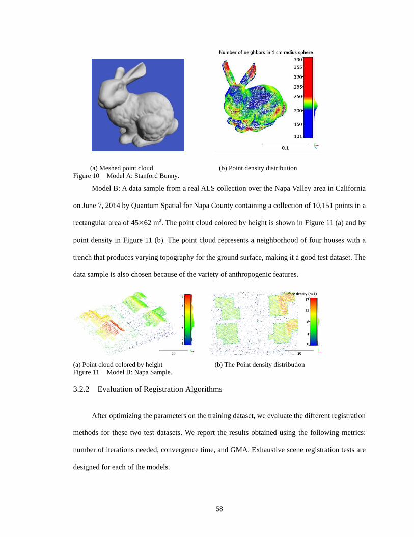
58

(a) Meshed point cloud (b) Point density distribution

Figure 10 Model A: Stanford Bunny.

Model B: A data sample from a real ALS collection over the Napa Valley area in California

on June 7, 2014 by Quantum Spatial for Napa County containing a collection of 10,151 points in a

rectangular area of 45×62 m2. The point cloud colored by height is shown in Figure 11 (a) and by

point density in Figure 11 (b). The point cloud represents a neighborhood of four houses with a

trench that produces varying topography for the ground surface, making it a good test dataset. The

data sample is also chosen because of the variety of anthropogenic features.

(a) Point cloud colored by height (b) The Point density distribution

Figure 11 Model B: Napa Sample.

3.2.2 Evaluation of Registration Algorithms

After optimizing the parameters on the training dataset, we evaluate the different registration

methods for these two test datasets. We report the results obtained using the following metrics:

number of iterations needed, convergence time, and GMA. Exhaustive scene registration tests are

designed for each of the models.

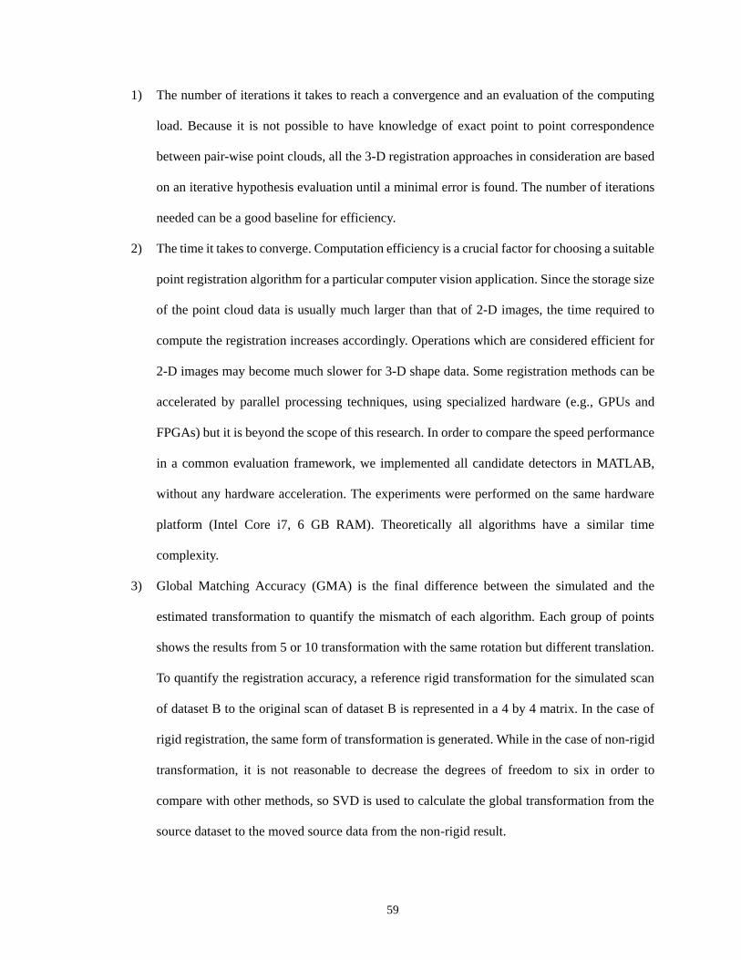
59

1) The number of iterations it takes to reach a convergence and an evaluation of the computing

load. Because it is not possible to have knowledge of exact point to point correspondence

between pair-wise point clouds, all the 3-D registration approaches in consideration are based

on an iterative hypothesis evaluation until a minimal error is found. The number of iterations

needed can be a good baseline for efficiency.

2) The time it takes to converge. Computation efficiency is a crucial factor for choosing a suitable

point registration algorithm for a particular computer vision application. Since the storage size

of the point cloud data is usually much larger than that of 2-D images, the time required to

compute the registration increases accordingly. Operations which are considered efficient for

2-D images may become much slower for 3-D shape data. Some registration methods can be

accelerated by parallel processing techniques, using specialized hardware (e.g., GPUs and

FPGAs) but it is beyond the scope of this research. In order to compare the speed performance

in a common evaluation framework, we implemented all candidate detectors in MATLAB,

without any hardware acceleration. The experiments were performed on the same hardware

platform (Intel Core i7, 6 GB RAM). Theoretically all algorithms have a similar time

complexity.

3) Global Matching Accuracy (GMA) is the final difference between the simulated and the

estimated transformation to quantify the mismatch of each algorithm. Each group of points

shows the results from 5 or 10 transformation with the same rotation but different translation.

To quantify the registration accuracy, a reference rigid transformation for the simulated scan

of dataset B to the original scan of dataset B is represented in a 4 by 4 matrix. In the case of

rigid registration, the same form of transformation is generated. While in the case of non-rigid

transformation, it is not reasonable to decrease the degrees of freedom to six in order to

compare with other methods, so SVD is used to calculate the global transformation from the

source dataset to the moved source data from the non-rigid result.

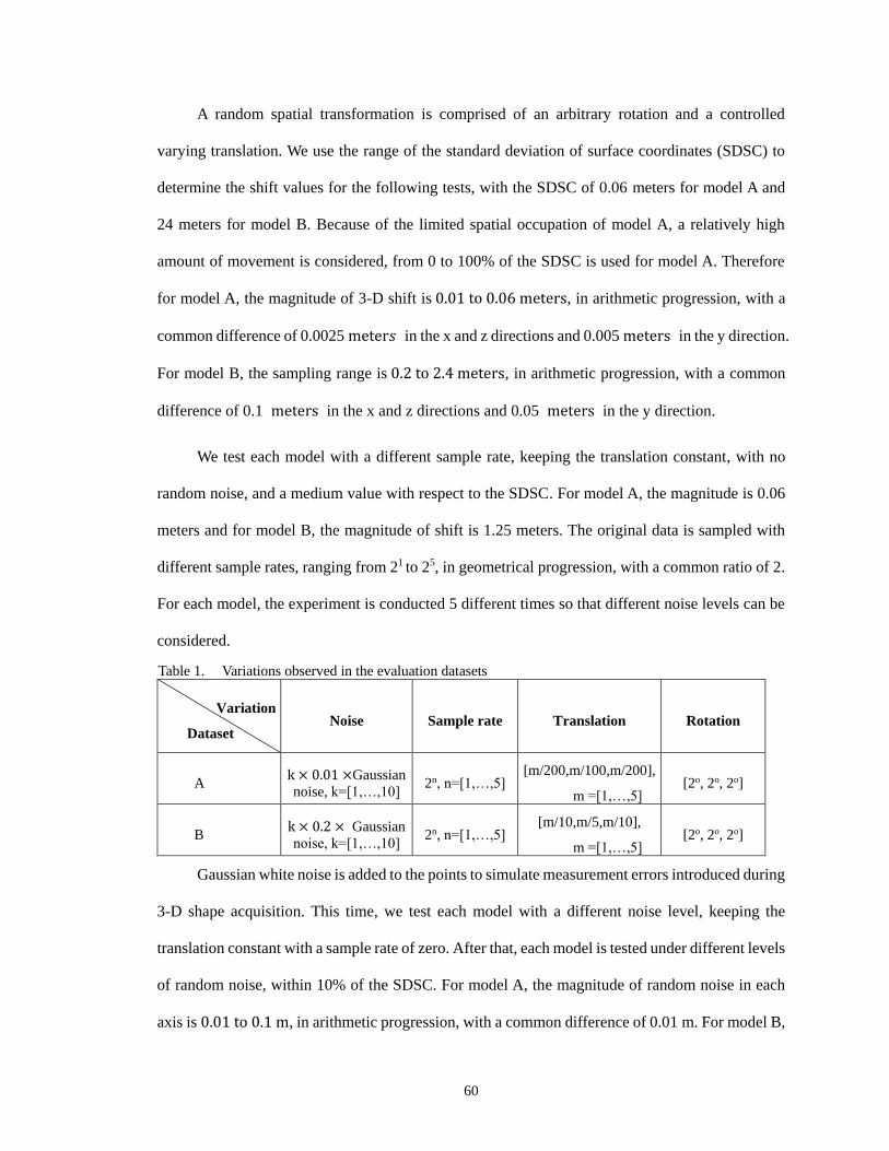
60

A random spatial transformation is comprised of an arbitrary rotation and a controlled

varying translation. We use the range of the standard deviation of surface coordinates (SDSC) to

determine the shift values for the following tests, with the SDSC of 0.06 meters for model A and

24 meters for model B. Because of the limited spatial occupation of model A, a relatively high

amount of movement is considered, from 0 to 100% of the SDSC is used for model A. Therefore

for model A, the magnitude of 3-D shift is 0.01 to 0.06 meters, in arithmetic progression, with a

common difference of 0.0025 meter𝑠 in the x and z directions and 0.005 meters in the y direction.

For model B, the sampling range is 0.2 to 2.4 meters, in arithmetic progression, with a common

difference of 0.1 meters in the x and z directions and 0.05 meters in the y direction.

We test each model with a different sample rate, keeping the translation constant, with no

random noise, and a medium value with respect to the SDSC. For model A, the magnitude is 0.06

meters and for model B, the magnitude of shift is 1.25 meters. The original data is sampled with

different sample rates, ranging from 21 to 25, in geometrical progression, with a common ratio of 2.

For each model, the experiment is conducted 5 different times so that different noise levels can be

considered.

Variation

Dataset Noise Sample rate Translation Rotation

A k × 0.01 ×Gaussian

noise, k=[1,…,10] 2n, n=[1,…,5]

[m/200,m/100,m/200],

m =[1,…,5] [2o, 2o, 2o]

B k × 0.2 × Gaussian

noise, k=[1,…,10] 2n, n=[1,…,5]

[m/10,m/5,m/10],

m =[1,…,5] [2o, 2o, 2o]

Gaussian white noise is added to the points to simulate measurement errors introduced during

3-D shape acquisition. This time, we test each model with a different noise level, keeping the

translation constant with a sample rate of zero. After that, each model is tested under different levels

of random noise, within 10% of the SDSC. For model A, the magnitude of random noise in each

axis is 0.01 to 0.1 m, in arithmetic progression, with a common difference of 0.01 m. For model B,

Table 1. Variations observed in the evaluation datasets

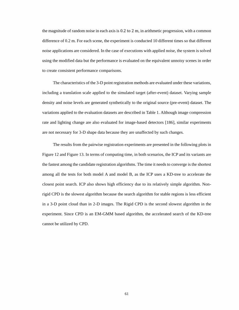
61

the magnitude of random noise in each axis is 0.2 to 2 m, in arithmetic progression, with a common

difference of 0.2 m. For each scene, the experiment is conducted 10 different times so that different

noise applications are considered. In the case of executions with applied noise, the system is solved

using the modified data but the performance is evaluated on the equivalent unnoisy scenes in order

to create consistent performance comparisons.

The characteristics of the 3-D point registration methods are evaluated under these variations,

including a translation scale applied to the simulated target (after-event) dataset. Varying sample

density and noise levels are generated synthetically to the original source (pre-event) dataset. The

variations applied to the evaluation datasets are described in Table 1. Although image compression

rate and lighting change are also evaluated for image-based detectors [186], similar experiments

are not necessary for 3-D shape data because they are unaffected by such changes.

The results from the pairwise registration experiments are presented in the following plots in

Figure 12 and Figure 13. In terms of computing time, in both scenarios, the ICP and its variants are

the fastest among the candidate registration algorithms. The time it needs to converge is the shortest

among all the tests for both model A and model B, as the ICP uses a KD-tree to accelerate the

closest point search. ICP also shows high efficiency due to its relatively simple algorithm. Non-

rigid CPD is the slowest algorithm because the search algorithm for stable regions is less efficient

in a 3-D point cloud than in 2-D images. The Rigid CPD is the second slowest algorithm in the

experiment. Since CPD is an EM-GMM based algorithm, the accelerated search of the KD-tree

cannot be utilized by CPD.

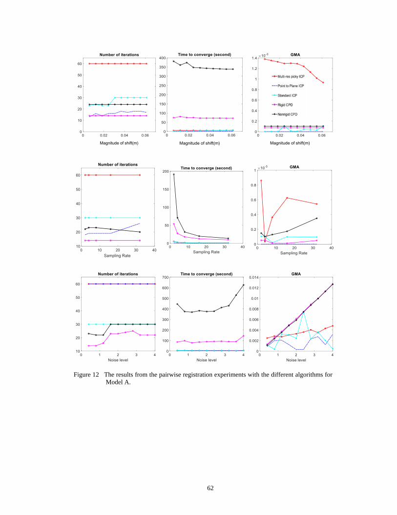
62

Figure 12 The results from the pairwise registration experiments with the different algorithms for

Model A.

Magnitude of shift(m) Magnitude of shift(m) Magnitude of shift(m)

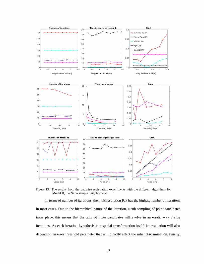
63

Figure 13 The results from the pairwise registration experiments with the different algorithms for

Model B, the Napa sample neighborhood.

In terms of number of iterations, the multiresolution ICP has the highest number of iterations

in most cases. Due to the hierarchical nature of the iteration, a sub-sampling of point candidates

takes place; this means that the ratio of inlier candidates will evolve in an erratic way during

iterations. As each iteration hypothesis is a spatial transformation itself, its evaluation will also

depend on an error threshold parameter that will directly affect the inlier discrimination. Finally,

Magnitude of shift(m) Magnitude of shift(m) Magnitude of shift(m)

64

for this same reason, shift range and data noise will also affect the system. Although the GMA is

within an acceptable range when the shift amount is less than 1 meter for model B, the GMA is

high compared to other methods when the same amount of noise is added. This will not happen

with a regular ICP approach as this method will implicitly select the elements in the payoff matrix

with less noise and the solution will be consistent regardless of how many different executions are

done. Subsampling has a huge impact on the performance after a certain point. For example, in the

case of model B, at a sample rate of 15, the GMA of multiresolution ICP is outstandingly poor due

to the insufficient number of points remaining.

In terms of registration accuracy, the GMA does not correspond to the change of sampling

rate for rigid and non-rigid CPD, for standard ICP and point to plane ICP, for either model A or B.

For model B, the GMA also stays stable and does not change much with the increase in shift amount

for any of the algorithms considered, i.e., rigid and non-rigid CPD, standard ICP and point to plane

ICP. Although the value of GMA does not seem as stable for these approaches for model A, all the

GMA values are under the level of 1.4 millimeters, which is less than 5% of the point cloud SDSC.

CPD does not tolerate noise well. Non-rigid CPD has an accurate registration result as the

value of GMA is near zero when there is no noise added to the data. On the other hand, when the

original data is corrupted with noise, even when the magnitude of the normal distribution is not

over 10% of the SDSC of the point cloud, the GMA is increased dramatically for both the non-rigid

and rigid CPD. Meanwhile, the GMA for ICP does not increase too much, the standard ICP is more

stable than point to plane minimum, and the difference in registration stays within the level of 0.03

for the transformation matrix, which is about 0.1 degree in rotation and 0.01 meters of translation.

That is clearly within the accuracy range of LiDAR point acquisition.

Overall, ICP with point to plane minimizing has a steady performance for model A. The mesh

is perfectly modelled from a uniform dense point cloud with almost continuous triangular faces

connecting vertices in all directions. A unique normal vector can be calculated for almost every

65

point in the model, leaving no freedom for sliding. Hence, it is not surprising that plain registration

methods can resolve a good global matching invariant of the magnitude of shift and sampling rate

in model A. However, for model B, by adding different levels of noise to the data, the plane-based

method failed to provide accurate results. This is because the roof tops have uniform normals

through the entire area, with space to freely slide parallel to the two planes, thusly making it easy

to fall into a local minimum. In the case of model A, which represents a uniformly high point

density, the standard ICP and point to plane ICP shows the best performance with the least

computation time and lowest average GMA throughout the tests that varied shift amounts and

sampling rates. ICP also shows decent robustness against different noise levels. In the case of model

B, which represents a locally varying density dataset that is more similar to the real ALS scanning

scenario, the standard ICP and point to plane ICP shows the best performance with the least

computing time and lowest average GMA throughout the tests that varied shift amounts and

sampling rates. Point to point ICP also shows better performance than point to plane ICP against

different noise levels.

66

4 DETAILED EXAMINATION OF ICP

From the testing results in Chapter 3, it can be concluded that standard ICP has stable and

robust performance. More precisely, experimental results obtained with the example datasets (Napa

sample), which included varying local density and multiple features, showed that when combining

a point to point minimizing error metric with a KD-tree searching acceleration method, the ICP

registration is ~25 times faster than CPD. The gain in speed is expected to be greater for bigger

datasets, due to the smaller complexity (O(Np)) of the ICP algorithm. ICP also successfully

maintains the range registration error under 5% when increasing the displacement between the test

data pair up to 10% of the average coordinate standard deviation. Furthermore, ICP is almost

invariant to increasing sample rate and noise level, which is the opposite of CPD. This clearly

shows that the proposed fast ICP algorithm exploits the fundamental nature of shape registration to

substantially improve its computational performance in the case of varying density ALS point

clouds with differing noise to the data ratios, while the plane-based method failed to provide

accurate results. Therefore, a detailed examination of the best method, ICP, using real ALS

scanning data will be undertaken.

4.1 ICP Refinements

When using ICP for near-fault earthquake deformation, the datasets are often surveyed over

large areas and the displacement is spatially varying with respect to the distance from the fault line.

It is not appropriate to consider it as a cohesive entity. Instead, the data should be first segmented

into smaller tiles that are suitable for rigid transformation. A moving window and tile-wise scheme

will be considered before implementing ICP for real data.

Because of the development of LiDAR technology, the legacy pre-event datasets usually

have a relatively sparse point spacing when compared to their newer, post-event counterparts. The

67

mismatch in point density will corrupt the registration accuracy, especially when the difference is

very large. This situation is often coupled with poor pre-event point accuracy resulting from the

higher flight altitude and less advanced ranging units used in legacy datasets. To address the

difficulties associated with sparse and low accuracy pre-event data, the proposed A-ICP method

incorporating spatially varying point accuracy will be considered to mitigate these problems. To

test the effect of weighting point pairs and the incorporation of point accuracy, the proposed A-ICP

and standard ICP will be compared first for a synthetic fault rupture.

4.2 Test Dataset

To better understand the effects of LiDAR point weighting, block size, moving windows, and

constraint conditions on displacements estimated using ICP and A-ICP, a series of tests were

performed using a synthetic deformation applied to an ALS point cloud acquired over the Henry

Mountains in Utah. The data was collected in 2008 by the National Center for Airborne Laser

Mapping (NCALM) using an Optech Gemini ALS system operated at a height of approximately

700 m above ground level. The raw ALS average point density is approximately 3.4 pts/m2. Only

one flight line (#17) over the area of the Milk Point River was used to create the synthetic dataset.

A single flight line was chosen to remove uncertainty due to overlap between LiDAR swaths,

allowing a more direct determination of the effect of point accuracy on displacement estimation.

The synthetic point clouds were created by first dividing the actual 2008 ALS data into two parts

along a randomly selected fault line, see Figure 14 (c). On each side of the fault line a uniform

movement of 2 m in the upward/downward (±∆z) direction is applied. Along with the constant shift,

3-D noise is added to each point. This was done by applying a gaussian noise generator, which has

minimum absolute value of 0.1 m and maximum of 1.0 m based on the estimated accuracy, across

the simulated data. Finally, based on the discussion in 3.1.2, the estimated point accuracy is

dominated by the scanning geometry and, therefore, uncertainty values were systematically

68

simulated for each point in flight line 17 using the scan angle of the laser scanner as the angle of

incidence (see Figure 8). The entire dataset is then broken down into tiles using the same boundaries

as the original data. Given the point density and topography, a tile size of 50 m by 50 m was used.

Figure 14 (a) Topography along flight line #17, (b) Synthetic LiDAR point accuracy, (c) Artificial

surface fault line creation.

4.3 Test Result and Discussion

Tile-wise ICP and A-ICP (both with a tile size of 50 m) are analyzed to test the effectiveness

of point accuracy as an anisotropic weighting factor. Arbitrary movements can exist for tiles

overlapping the surface rupture as they may contain all or part of the fault trace, and therefore these

tiles were not evaluated. The results are presented with consideration for the following definitions:

Qu is defined as the mean difference for every data tile calculated by differencing the

original data block and the transformed data block using the estimated rigid body

transformation.

ER is defined as the RMS of errors, estimated from the correspondence of point to point

distance, of the converged point or of the last iteration, with an allowed maximum number

of iterations of 200 and convergence tolerance of 1e-6.

The actual movement is known and thus the reference value for Qu is known and therefore

the results from ICP and A-ICP are compared with the reference Qu. A comparison of the results

from ICP and A-ICP against the known displacement are given in Figure 16 and Table 2. The mean

ER for the last iteration is 0.66 m for ICP and 0.44 m for A-ICP. The mean number of iterations for

69

convergence is 29 for A-ICP and 35 for ICP. Overall, A-ICP better estimates the actual movement

as indicated in Table 2 with better Qu consistency and data dispersion. A-ICP also shows only slight

degradation in the results for the tiles with higher uncertainty (Figure 16), while ICP introduces

noise in the horizontal displacement estimates even in tiles with a low level of estimated uncertainty.

Determination of Optimal Window and Step Size

Result Mapping

Reference dataset

TestWindow Size

/Step Size

Target dataset

Spatial Scope

Density

Valid number of points

Data within current window

A-ICPWindow Moving

Accuracy Estimation

3D Point Accuracy

Figure 15 Flow chart for moving window A-ICP. The brown box highlights the iterative process to

determine the optimal window size and step size by considering the data density, the number

of points required for an accurate estimation, and the expected spatial scale and nature of the

deformation.

The flowchart for moving window A-ICP is given in Figure 15 and the process for

determination of the optimal moving window size is highlighted in the flowchart.

Table 2 Comparison of ICP and A-ICP against reference movement for flight line #17 and moving

window ICP and A-ICP against the reference for the entire dataset (results in meters).

Flight Line #17 Only Entire Dataset

Method ICP A-ICP Moving ICP Moving A-ICP

Axis x z x z x z x z

Mean of Difference

in Qu (m)

-0.122 -0.019 -0.074 -0.060 -0.004 0.030 -0.002 0.027

STD of Difference

in Qu (m)

0.623 0.458 0.631 0.436 0.693 0.122 0.681 0.118

Mean of Absolute

Difference in Qu

(m)

0.331 0.469 0.328 0.339 0.472 0.061 0.437 0.056

Mean ER of Last

Iteration (m)

0.66 0.44 0.211 0.197

Mean # of

Iteration

35 29 35 30

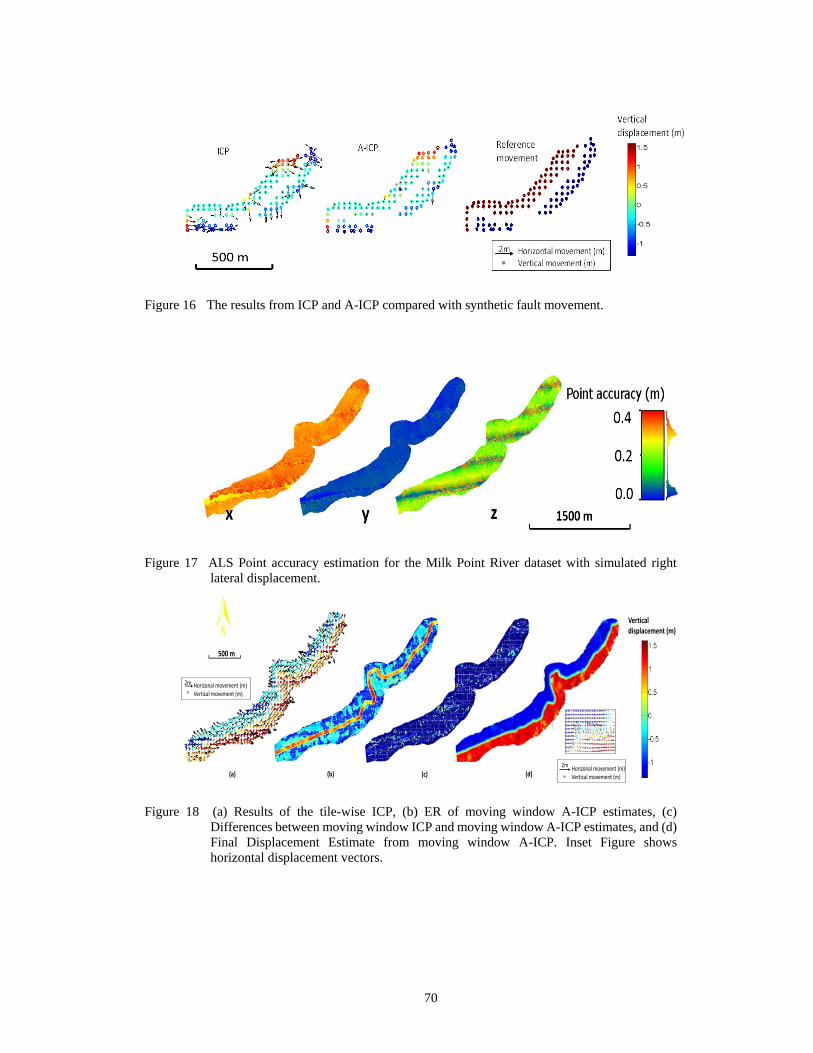
70

Figure 16 The results from ICP and A-ICP compared with synthetic fault movement.

Figure 17 ALS Point accuracy estimation for the Milk Point River dataset with simulated right

lateral displacement.

Figure 18 (a) Results of the tile-wise ICP, (b) ER of moving window A-ICP estimates, (c)

Differences between moving window ICP and moving window A-ICP estimates, and (d)

Final Displacement Estimate from moving window A-ICP. Inset Figure shows

horizontal displacement vectors.

(a) (c)(b)

Vertical displacement (m)

(d)

500 m

2m Horizonal movement (m)Vertical movement (m)

2m Horizonal movement (m)Vertical movement (m)

71

(a) Outlined area of ER>0.5 (b) Refinement result of ICP with smaller window

Figure 19 Refinement of near-fault rupture displacement.

Each moving window block adopts a fractional portion of the new point cloud information

when estimating change and therefore outliers can be easily removed and the final deformation

result will be smoother. To test the use of a moving window, a deformation assessment using the

entire Milk Point River dataset with the simulated rupture is performed. On each side of the fault

line a uniform movement of 2 m to the east/west (±Δx) and 2 m in the upward/downward (±Δz)

direction is applied, simulating a right lateral fault, with estimated point accuracy derived for all of

the LiDAR points (Figure 17). Moving windows of the same size (50 m by 50 m), but with a step

size smaller than the block size (10 m), are used to provide overlapping estimates. Most of the

abnormalities in the tile-wise standard ICP estimates are along the synthetic fault line or adjacent

to the dataset boundary (see Figure 18 (a)). From Figure 18 (c), the differences between moving

window A-ICP and ICP are located mostly at positions with poorer LiDAR point accuracy (see

point accuracy estimation in Figure 17), where we have shown previously that A-ICP provides

better estimates because of the anisotropic weighting criteria. Table 2 shows that moving window

A-ICP maintains an advantage in Qu consistency and time efficiency over ICP. The final estimates

for moving window A-ICP results are given in Figure 18 (d). The moving window obviously shows

more detail and crisp delineation of the simulated fault; the resolved systematic noise has overcome

ER(m)

72

the error pattern of the estimated point accuracy (Figure 17). Based on these comparisons, it appears

that the moving window A-ICP gives the best performance for detecting fault lines and estimating

topographic movement.

The final values of ER for the moving window A-ICP estimation, Figure 18 (b), provide a

fine delineation of the fault location. The higher values of ER along the rupture indicate the tiles

that straddle the fault and therefore cause higher residuals and estimated uncertainty in the final

deformation estimate for that tile. Therefore, the final ER values could be used as an indicator of

surface rupture location. To confirm this assumption, the area where ER values are over the

threshold of 0.5 is outlined in black color in Figure 19 (a). LiDAR points that fall into this area are

used, instead of the entire dataset, to refine the result, with a finer window size of 20 m and a

moving step of 5 m. A refined detail and more crisp delineation of the simulated fault is shown in

Figure 19 (b). Although because the size of window is not optimized, some of the tiles have an

insufficient number of points for the ICP calculation. However, this result confirms the ability of

A-ICP to refine near-fault deformation with the flexibility of the moving window approach. The

results show that the moving window A-ICP gives the best performance for estimating topographic

movement for large scale topography and also has the ability to enhance finer near-fault

deformation estimates with dynamic window size and moving steps. Therefore, to estimate 3-D

near-fault deformation on real data, A-ICP with a moving window will be used as the registration

method and a similar coarse to fine resolution scheme can be used to enhance deformation estimates

and find additional, smaller near-fault surface ruptures.

A-ICP algorithms in particular can mitigate error from GNSS measurements inherent in

airborne laser scanning, and have the potential to correct the errors caused by moving or poorly

modeled survey targets or monuments, all of which have the potential to affect landscape change

detection significantly. Difficulties associated with sparse legacy pre-event datasets and

73

anthropogenic change in the near-fault landscape will be further discussed in each study case

presented in Chapter 5.

4.4 Sources and Magnitudes of Error

Although creating error budgets for differential analyses from multi-temporal, high-

resolution, 3-D data is challenging, we can discuss the factors that determine the reliability of our

A-ICP change detection. The principal sources of error are: (1) inherent laser scanner error and (2)

the effectiveness of the A-ICP algorithm that was used to refine internal alignment among scan

positions within a scan epoch and to align the multi-temporal point clouds between scan epochs.

All errors from the LiDAR measurements are estimated using an accuracy estimation model

with GNSS and IMU trajectories (3.1.2). However, this part of the error is mitigated by the use of

the A-ICP algorithm. There is no expectation that a point cloud of an object would have the same

exact internal structure if the object was scanned at two times or from two locations; so the use of

rigid body modeling removes any effect of point cloud heterogeneity within the point cloud inside

a given moving window.

The error introduced by the A-ICP algorithm is not simple to quantify. An estimation of error

propagation through the point cloud to the registered point cloud can be performed to an

approximate level. A close-form of covariance of ICP registration is proposed in [187] for a 2-D

point cloud registration. Later [188] extended this work for 3-D point cloud registration. However,

these papers do not consider the possibility of noise being present in the three variables present in

3-D.

The implementation is a generalized method for 3-D ICP covariance estimation without any

constraints on rotation and translation. The approximate value of the covariance matrix of the

estimates, X= [x y z a b c], is the ICP’s transformation estimate where z represents the n sets of the

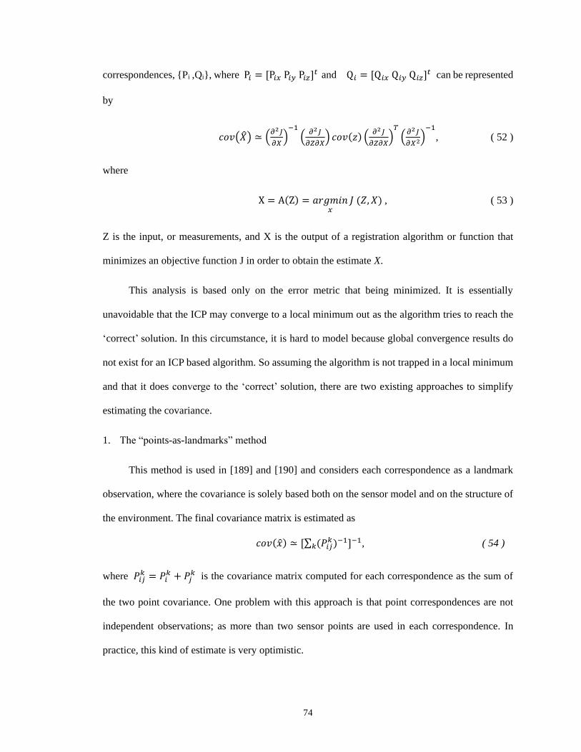
74

correspondences, {Pi ,Qi}, where P𝑖 = [P𝑖𝑥 P𝑖𝑦 P𝑖𝑧]𝑡

and Q𝑖 = [Q𝑖𝑥 Q𝑖𝑦 Q𝑖𝑧]𝑡 can be represented

by

𝑐𝑜𝑣(�̂�) ≃ (𝜕2𝐽

𝜕𝑋)−1

(𝜕2𝐽

𝜕𝑍𝜕𝑋) 𝑐𝑜𝑣(𝑧) (

𝜕2𝐽

𝜕𝑍𝜕𝑋)𝑇

(𝜕2𝐽

𝜕𝑋2)−1

, ( 52 )

where

X = A(Z) = 𝑎𝑟𝑔𝑚𝑖𝑛𝑥

𝐽 (𝑍, 𝑋) , ( 53 )

Z is the input, or measurements, and X is the output of a registration algorithm or function that

minimizes an objective function J in order to obtain the estimate X.

This analysis is based only on the error metric that being minimized. It is essentially

unavoidable that the ICP may converge to a local minimum out as the algorithm tries to reach the

‘correct’ solution. In this circumstance, it is hard to model because global convergence results do

not exist for an ICP based algorithm. So assuming the algorithm is not trapped in a local minimum

and that it does converge to the ‘correct’ solution, there are two existing approaches to simplify

estimating the covariance.

1. The “points-as-landmarks” method

This method is used in [189] and [190] and considers each correspondence as a landmark

observation, where the covariance is solely based both on the sensor model and on the structure of

the environment. The final covariance matrix is estimated as

𝑐𝑜𝑣(�̂�) ≃ [∑ (𝑃𝑖𝑗𝑘)−1

𝑘 ]−1, ( 54 )

where 𝑃𝑖𝑗𝑘 = 𝑃𝑖

𝑘 + 𝑃𝑗𝑘 is the covariance matrix computed for each correspondence as the sum of

the two point covariance. One problem with this approach is that point correspondences are not

independent observations; as more than two sensor points are used in each correspondence. In

practice, this kind of estimate is very optimistic.

75

2. The “Hessian” method

The “Hessian” method, proposed in [1], suggests that, if the objective function was a

quadratic as

𝐽 = (𝑌 − 𝑀𝑋)𝑇(𝑌 − 𝑀𝑋), ( 55 )

then the covariance of registration estimate, �̂� = (𝑀𝑇𝑀)−1𝑀𝑇𝑌, can be simplified to

𝑐𝑜𝑣(�̂�) ≃ (1

2

𝜕2𝐽

𝜕𝑋2)−1 𝜎2. ( 56 )

The unbiased estimate 𝑠2 of 𝜎2 = 𝐽/(𝐾 − 3), where 𝐾 is the number of correspondences

and J is the objective function at the final iteration, is

𝐽 = ∑ ‖𝑅𝑃𝑖 − 𝑇 − 𝑄𝑖‖2

𝑖 . ( 57 )

[188] shows that this method in some cases overestimates the true covariance. However, it gives

an accountable boundary of accuracy for the registration. The first term of covariance can be

described as

(𝜕2𝐽

𝜕𝑥2)−1

=

[

𝑑2𝐽

𝑑𝑥2

𝑑2𝐽

𝑑𝑦2

𝑑2𝐽

𝑑𝑧2

𝑑2𝐽

𝑑𝑎2

𝑑2𝐽

𝑑𝑏2

𝑑2𝐽

𝑑𝑐2

𝑑2𝐽

𝑑𝑎𝑑𝑦

𝑑2𝐽

𝑑𝑧𝑑𝑎

𝑑2𝐽

𝑑𝑎𝑑𝑧

𝑑2𝐽

𝑑𝑦𝑑𝑥

𝑑2𝐽

𝑑𝑥𝑑𝑦

𝑑2𝐽

𝑑𝑧𝑑𝑥

𝑑2𝐽

𝑑𝑥𝑑𝑎

𝑑2𝐽

𝑑𝑎𝑑𝑥

𝑑2𝐽

𝑑𝑦𝑑𝑎

𝑑2𝐽

𝑑𝑥𝑑𝑏

𝑑2𝐽

𝑑𝑏𝑑𝑥

𝑑2𝐽

𝑑𝑦𝑑𝑏

𝑑2𝐽

𝑑𝑏𝑑𝑦

𝑑2𝐽

𝑑𝑧𝑑𝑏

𝑑2𝐽

𝑑𝑏𝑑𝑧

𝑑2𝐽

𝑑𝑐𝑑𝑦

𝑑2𝐽

𝑑𝑧𝑑𝑐

𝑑2𝐽

𝑑𝑐𝑑𝑧

𝑑2𝐽

𝑑𝑐𝑑𝑏

𝑑2𝐽

𝑑𝑐𝑑𝑎

𝑑2𝐽

𝑑𝑎𝑑𝑐

𝑑2𝐽

𝑑𝑥𝑑𝑐

𝑑2𝐽

𝑑𝑐𝑑𝑥

𝑑2𝐽

𝑑𝑦𝑑𝑐

𝑑2𝐽

𝑑𝑎𝑑𝑏

𝑑2𝐽

𝑑𝑏𝑑𝑎

𝑑2𝐽

𝑑𝑏𝑑𝑐

𝑑2𝐽

𝑑𝑥𝑑𝑧

𝑑2𝐽

𝑑𝑦𝑑𝑧

𝑑2𝐽

𝑑𝑧𝑑𝑦]

. ( 58 )

3. A-ICP error estimation and propagation

It should be noted that the standard ICP cannot avoid the error source from sensor noise or

scanning mechanism; this error is independent of the registration error. The result of the comparison

between ICP and A-ICP on the experimental dataset in 4.2 confirms this. However, this error is

justified by the weighting approach in A-ICP using the fiducial error metric. Here, in the case of

weighted ICP, a new covariance matrix can be written as

76

𝑐𝑜𝑣(�̂�) ≃ 2𝑊 (𝜕2𝐽

𝜕𝑥2)−1

𝜎2𝑊𝑇 and ( 59 )

𝑊 = 𝑑𝑖𝑎𝑔 [ 𝜎𝑝𝑥2, 𝜎𝑞𝑦

2, 𝜎𝑝𝑧2, 𝜎𝑝𝑥

2, 𝜎𝑝𝑦2, 𝜎𝑝𝑧

2]−1. ( 60 )

Now, with 𝑐𝑜𝑣(�̂�), the variance of position can be calculated by

𝑃𝐴 = 𝑊(𝑅𝑃𝑖 − 𝑇) = 𝐴 (𝑅

𝑇) = 𝐴(�̂�) , ( 61 )

where P𝐴 is the new position acquired after applying A-ICP. The covariance of an algebraic

expression of the form Bz+c, where c is a constant, is 𝐵𝑐𝑜𝑣(𝑧)𝐵𝑇. Applying this property, the result

of covariance of the new after position A-ICP registration can be expressed as

𝑐𝑜𝑣(𝑋𝑃𝐴̂ ) = (

𝜕𝐴

𝜕(𝑅/𝑇))𝑐𝑜𝑣(�̂�)(

𝜕𝐴

𝜕(𝑅/𝑇))𝑇

= (𝜕𝐴

𝜕(�̂�))𝑐𝑜𝑣(�̂�)(

𝜕𝐴

𝜕(�̂�))𝑇. ( 62 )

The comparison results from 4.3 show that the moving window A-ICP gives the best performance

for estimating topographic movement for large scale topography and also has the ability to enhance

finer near-fault deformation estimates with dynamic window size and moving steps. The modeling

of A-ICP error estimation and propagation to the new position provide a rigorous error analysis of

the algorithm. For the application of A-ICP with accessible point accuracy estimation, the accuracy

of A-ICP change detection can be estimated. One important point to note is that only the

correspondences in the final iteration are used for the covariance estimation in the provided

implementation, so that other variants that might change how the final step is reached are not

considered here.

77

5 CASE STUDY ON SURFACE RUPTURES

Two case studies, to show how the proposed 3-D change detection methods can be used to

estimate real ALS measured earthquake deformation and to identify and resolve specific problems

encountered when dealing with real data, are shown in this chapter. These problems include: (1)

addressing the difficulties associated with sparse legacy pre-event datasets by incorporating point

accuracy estimation into the ICP adjustment, and (2) anthropogenic change of the landscape, in

which possible methods to make full use of the multi-return and classified point cloud are

introduced to optimize the solution for near-fault displacements.

5.1 El Mayor Earthquake

On April 4, 2010 a Mw 7.2 earthquake occurred in Baja California, Mexico (see the Shake

Map for the earthquake in [191]). This earthquake is normally referred to as the El Mayor-Cucapah

(EMC) earthquake. A 120 kilometer stretch of the resultant surface rupture was covered by both

pre- and post-earthquake ALS [76]. To rigorously determine spatial change near the major fault

lines of the EMC earthquake, we implemented the anisotropic weighted ICP (A-ICP) algorithm,

which was initially introduced in Chapter 2, and modeled the random error for every LiDAR

observation in the differential point cloud for use as a priori weights in the ICP algorithm. The

implementation is evaluated by first qualitatively and quantitatively comparing the performance of

the standard ICP and A-ICP algorithms. To further enhance the spatial resolution, we implemented

a moving window technique for the A-ICP analysis. Practical application of the moving window

A-ICP technique is evaluated by estimating post-earthquake slip for the 2010 El Mayor-Cucapah

Earthquake (EMC) using pre- and post-event LiDAR and comparing the estimated surface

displacement to in-situ field observations of displacement.

78

5.1.1 Airborne Dataset Description

The specifications of the pre- and post-EMC earthquake ALS datasets are given in Table 3.

A full description and the approximate coverage of the datasets can be found in [13]. There is a

large point density disparity between pre- and post-event datasets; the post-event dataset is ~1000

times as dense as the pre-event dataset. A surface-based matching approach may not give ideal

results because the two surface models have to have been developed and registered to the same grid

tessellation for comparison. This will result in an inevitable loss of information and an addition of

noise when the higher resolution surface is down sampled or the lower resolution surface is

interpolated. However, the data disparity has minimal influence on the performance of CPC-based

approaches such as ICP 3-D change detection because the scale of the expected deformation is still

larger than the coarser point density of the pre-event dataset.

Table 3. Specifications of the pre- and post-event ALS datasets covering the surface rupture of the EMC

earthquake

Name Pre-event Post- event

Time 31 Jul–7 Aug 2006 16–19 Aug 2010

Acquisition Agency Instituto Nacional de Estadística y

Geografía (INEGI)

National Center for Airborne

Laser Mapping (NCALM)

Aircraft Flying Altitude 6000m 600m

Aircraft Flying Speed 100 m/s 80 m/s

Laser Scanner Model Leica ALS40 Optech Gemini

Pulse Rate 16 kHz 100 kHz

Scan Angle ±32° ±14°

Flight Lines 16 north-south lines w/ 30% side overlap 24 lines w/50% side overlap

Point Density 0.013 points/m2 10 points/m2

The GPS reference datum for the 2006 INEGI flights and the 2010 NCALM flights was

different and therefore a common occurrence for temporally spaced ALS collections. Geodetic

preprocessing using HTDP (Horizontal Time-Dependent Positioning) [192] was utilized to update

the INEGI survey datum (ITRF92 with an epoch date of 1988.000) to the NCALM flight datum

(ITRF2000 with an epoch date of 2010.627). This datum change resulted in a coordinate shift of

79

approximately 0.900, 0.429, and 0.004 m (east, north, and up) and was applied to the original

INEGI data [13].

5.1.2 Methods

Based on Chapter 4, we can conclude that, for a synthetic deformation with random noise

added to the ALS point cloud, A-ICP better estimates the actual movement with better Qu

consistency and data dispersion and only shows slight degradation in the results for the tiles with

higher uncertainty, while standard ICP introduces noise into the horizontal displacement estimates

even in tiles with a low level of estimated uncertainty. The pre-event ALS survey for the EMC

earthquake has poorer point accuracy and sparser point density compared to the post-event ALS

dataset. These difficulties could be overcome by using A-ICP with estimated point accuracy because

A-ICP provides better estimates due to the anisotropic weighting criteria, as shown in Table 2.

The flowchart for moving window A-ICP is given in Figure 15 and the process for

determining the optimal moving window size is highlighted in the flowchart. To ensure we were

not missing local deformation and to maintain a sufficient number of points within each window,

tests with different window sizes (including 50, 100, 200, and 400 m) with a step size of ¼ of the

window size were performed. The convergence error and convergence time for A-ICP did not

significantly improve as the window size decreased and no localized deformations at the smaller

window sizes were evident; therefore, a 400 m window was used. Each moving window block

adopts a fractional amount of new point cloud information when estimating change and therefore

outliers can be easily removed resulting in a smoother final estimate of deformation. The final ER

values can also be used as an indicator of surface rupture location.

To use A-ICP for the EMC earthquake change detection, we need to consider LiDAR point

accuracy. The weighted point accuracy is dominated by the uncertainty in the pre-event dataset

because it was flown at a lower point density and at a significantly higher altitude and, therefore,

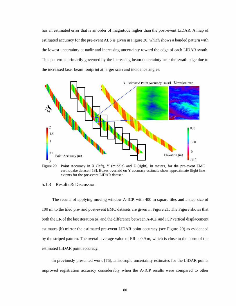
80

has an estimated error that is an order of magnitude higher than the post-event LiDAR. A map of

estimated accuracy for the pre-event ALS is given in Figure 20, which shows a banded pattern with

the lowest uncertainty at nadir and increasing uncertainty toward the edge of each LiDAR swath.

This pattern is primarily governed by the increasing beam uncertainty near the swath edge due to

the increased laser beam footprint at larger scan and incidence angles.

Figure 20 Point Accuracy in X (left), Y (middle) and Z (right), in meters, for the pre-event EMC

earthquake dataset [13]. Boxes overlaid on Y accuracy estimate show approximate flight line

extents for the pre-event LiDAR dataset.

5.1.3 Results & Discussion

The results of applying moving window A-ICP, with 400 m square tiles and a step size of

100 m, to the tiled pre- and post-event EMC datasets are given in Figure 21. The Figure shows that

both the ER of the last iteration (a) and the difference between A-ICP and ICP vertical displacement

estimates (b) mirror the estimated pre-event LiDAR point accuracy (see Figure 20) as evidenced

by the striped pattern. The overall average value of ER is 0.9 m, which is close to the norm of the

estimated LiDAR point accuracy.

In previously presented work [76], anisotropic uncertainty estimates for the LiDAR points

improved registration accuracy considerably when the A-ICP results were compared to other

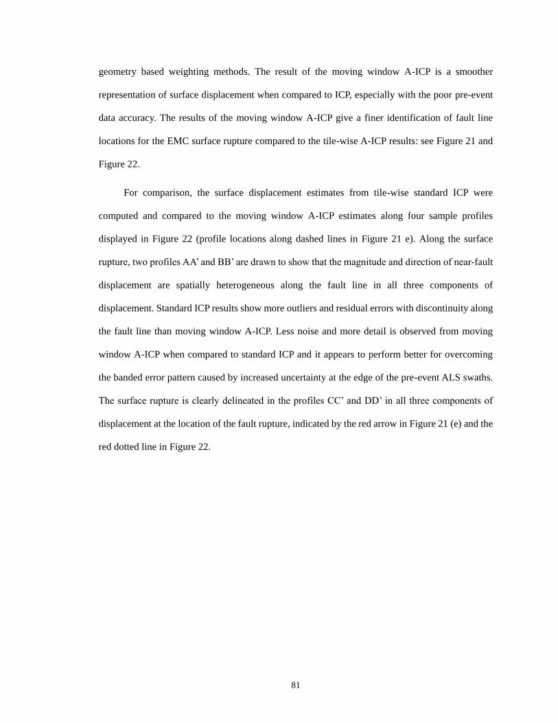
81

geometry based weighting methods. The result of the moving window A-ICP is a smoother

representation of surface displacement when compared to ICP, especially with the poor pre-event

data accuracy. The results of the moving window A-ICP give a finer identification of fault line

locations for the EMC surface rupture compared to the tile-wise A-ICP results: see Figure 21 and

Figure 22.

For comparison, the surface displacement estimates from tile-wise standard ICP were

computed and compared to the moving window A-ICP estimates along four sample profiles

displayed in Figure 22 (profile locations along dashed lines in Figure 21 e). Along the surface

rupture, two profiles AA’ and BB’ are drawn to show that the magnitude and direction of near-fault

displacement are spatially heterogeneous along the fault line in all three components of

displacement. Standard ICP results show more outliers and residual errors with discontinuity along

the fault line than moving window A-ICP. Less noise and more detail is observed from moving

window A-ICP when compared to standard ICP and it appears to perform better for overcoming

the banded error pattern caused by increased uncertainty at the edge of the pre-event ALS swaths.

The surface rupture is clearly delineated in the profiles CC’ and DD’ in all three components of

displacement at the location of the fault rupture, indicated by the red arrow in Figure 21 (e) and the

red dotted line in Figure 22.

83

Figure 21 Moving window A-ICP estimates of displacement for the EMC earthquake. (a) ER of last iteration, (b) Difference between moving window A-ICP

and moving window ICP vertical displacement estimates (c) Final moving window A-ICP estimate of horizontal surface displacement in X, (d) A-

ICP estimate of horizontal surface displacement in Y, (e) A-ICP estimate of vertical surface displacement in Z, with locations of major surface

ruptures and profiles overlaid on A-ICP estimate of vertical surface displacement, and scale of displacement field is indicated in color scale from

blue to red.

84

The standard ICP results show additional residual errors in the displacement estimates that

are correlated with flight line placement; they are predominantly at the edge of the flight line swaths

where any remaining laser misalignment or boresight errors would be magnified [13]. The vertical

and horizontal components of the estimated displacement field from moving window A-ICP show

more spatially varying surface movements across the fault lines than the estimates from standard

tile-wise ICP, while still maintaining the major features of the fault movement.

Figure 22 Four representative profiles of the estimated displacement field in horizontal direction (dx and

dy), and vertical direction, dz. Standard ICP (red) and moving window A-ICP (blue). The red

dotted lines on profile CC’ and DD’ show the surface delineation in all three components of

displacement at the location of the fault rupture, indicated by the red arrows in Figure 21.

85

Fault slip and distributed earthquake-driven deformation in the surrounding volume are now

well imaged in the resulting A-ICP displacement fields (Figure 21 c - e). Vertical displacements

can be clearly observed dominating the important Paso Inferior accommodation zone in the north-

western portion of the rupture but a significant right-lateral motion is also evident from the

horizontal displacement estimates. The overall ALS near-fault displacements agree with detailed

field mapping undertaken in this area [193] but the comparison of the field measurements and the

3-D LiDAR differencing results need to be quantitatively presented and analyzed in order to

confirm the closeness of agreement.

Fortunately, field investigation is often carried out after a significant earthquake. The

measurement of offset parallel to the fault trace, including the strike-slip and vertical components,

can generally be made at a limited number of sites where natural or anthropogenic features which

used to be continuous across the fault zone, have been clearly offset by a measurable amount [194].

However, even in favorable cases, the uncertainty in the feature geometry before seismic

deformation leads to considerable uncertainty in the measurement of seismic displacement across

the fault zone [195]. Other uncertainty factors, such as time delay, subjectivity of survey site

selections, temporal decorrelation due to material settling, and false interpretation of fault behaviors

will also contribute to uncertainty in field measurements. These uncertainties are the reason that

most studies only use the field rupture location to constrain the fault rupture trace, while rarely

adopting the field rupture displacement estimates into the dislocation model [196]. However, the

surface rupture offset measurements represent the displacements closest to the fault, where there is

normally no other available displacement estimate. Therefore, they are the only good basis for

comparison to the 3-D slip estimates from A-ICP. With a proper interpolation of the A-ICP results,

a comparison of “ground truth” from field measurements was conducted and the results are given

in Figure 24.

86

Figure 23 Field transect profile locations overlaid on the A-ICP results of vertical displacement.

Field measurements are shown in Table 4 for the EMC earthquake. They are taken from

supplement file 6 in [197]. The locations of the field measurements are overlaid on the A-ICP

vertical displacement estimates in Figure 23. 49 observations were taken from the field

measurements, and 41 that reside within the ALS coverage were used for comparison. Table 4 uses

“Lateral” to describe strike-slip, “Heave” as Heave, “Vertical” to describe Vertical throw, and “total”

to indicate the total displacement (A) calculated based on these three vectors:

𝐴 = √𝐿𝑎𝑡𝑒𝑟𝑎𝑙2 + 𝐻𝑒𝑎𝑣𝑒2 + 𝑉𝑒𝑟𝑡𝑖𝑐𝑎𝑙2. ( 63 )

The strike-slip orientation is different for every scarp measurement; therefore, a direct

comparison to the Qu calculated from ICP/ A-ICP is not realistic. However, vertical throw is

comparable to delta z and the horizontal displacement and total displacement should be comparable.

87

Table 4 SF6-1 from [197]. Field measurements of south Napa surface rupture.

Figure 24 Differences between ALS differential estimates and EMC field measurements at the

corresponding distance of ICP window center from locations of field measurements the

rupture trace. Estimated accuracy of the A-ICP estimates are given as red (vertical) and blue

(horizontal) bands in the figure. They represent 1σ values.

88

Figure 24 displays the results of the comparison between horizontal and vertical

displacement estimates from field measurements and various ICP approaches. The X axis in Figure

24 denotes the distance between the field measurements and the center of the ICP window closest

to the measurement site. Vertical differences in red and the horizontal differences in blue, marked

by circle (tile wise ICP), asterisk (moving window ICP), and diamond (moving window A-ICP).

Estimated accuracy of the A-ICP estimates are given as red (vertical) and blue (horizontal) bands

in the figure. They represent 1σ values.

The mean values of differences between the moving window A-ICP estimates and the field

measurements are near zero for both horizontal and vertical displacements. However, the tile-wise

and moving window ICP both have significant mean offsets in the horizontal direction of ~0.6 m.

The RMSE of the moving window A-ICP vertical differences is 0.464 m and the RMSE of the

horizontal differences is 0.648 m as shown in Table 5.

Table 5 The statistics of differences between ALS differential estimates using tile wise ICP, moving

window ICP, and moving window A-ICP results and field measurements of displacement from

the EMC earthquake.

The ratio of the vertical and horizontal differences is consistent with the mean error of the

pre-event A-ICP estimation as well as the mean error of LiDAR point accuracy, suggesting that the

offsets generally agree with the localized measurements in the field. Overall, the moving window

A-ICP results have a better agreement with field measurements than tile wise ICP and moving

window ICP, demonstrating the value of weighting the pre-event data using point accuracy. There

are numerous possibilities for the larger deviation in horizontal difference between A-ICP and field

Method Direction Mean (m) Standard deviation (m) RMSE (m)

Tile wise ICP Vertical -0.167 0.536 0.561

Horizontal -0.600 0.580 0.835

Moving window ICP Vertical -0.058 0.461 0.464

Horizontal -0.581 0.565 0.811

Moving window A-ICP Vertical -0.094 0.459 0.468

Horizontal -0.056 0.645 0.648

89

measurements, however the most probable are higher uncertainty in LiDAR horizontal point

location and ambiguity in field determined horizontal offsets. The A-ICP slip distribution and near-

fault displacements compare well with field measurements at the sub-meter scale but reveal local

discrepancies. The plotted horizontal and vertical differences are less than the mean accuracy of

the A-ICP estimates.

An independent samples t-test was conducted to compare the differences between the moving

window A-ICP estimates and the field measurements versus the differences between the tile wise

ICP estimates and the field measurements. These tests (both horizontal and vertical) will show

whether or not there is a significant difference between the compared two groups’ differences. The

independent samples t-test results indicates that there was a significant difference in the horizontal

differences between moving window A-ICP (mean=-0.056m, RMSE=0.648) and tile wise ICP

(mean=-0.600m, RMSE =0.835m); t (48) = 3.0734, p =0.0035. There was not a significant

difference in the vertical differences between moving window A-ICP (mean=-0.094m,

RMSE=0.468m) and tile wise ICP (mean=-0.167m, RMSE =0.568m); t (48) = 0.5016, p =0.6182.

This indicates that moving window A-ICP does have a significantly better horizontal agreement

with the field measurements compared to tile wise ICP, while only showing a slight improvement

in the vertical. There are two possible explanations for these results.. Within the optimized moving

window size of 400m, the vertical registration and the change detection results are expected to be

more accurate, because the vertical feature space is better defined than the horizontal. Second, the

vertical point uncertainty is smaller than the horizontal uncertainty, providing a more homogenous

distribution in estimated accuracy, and thus less difference in the weight for registration in the Z

direction. This uniformity in anisotropic accuracy distribution result in smaller vertical differences

between moving window A-ICP and tile wise ICP change detection results.

An independent samples t-test was also conducted to compare the differences between the

moving window ICP estimates and the field measurements versus the differences between the tile

90

wise ICP estimates and the field measurements. There was very little difference in the horizontal

differences for moving window ICP (mean = -0.581m, RMSE = 0.811m) and tile wise ICP (mean

= -0.600m, RMSE = 0.835); t (48) = 0.1147, p = 0.9092. There was also not a significant difference

in the vertical differences for moving window ICP (mean = -0.058m, RMSE = 0.464m) and tile

wise ICP (mean = -0.167m, RMSE = 0.561m); t (48) = 0.7543, p = 0.4544. These results show that

moving window ICP does not provide a significantly better horizontal or vertical agreement with

the field measurements when compared to tile wise ICP. While the moving window was able to

provide marginal improvement in the agreement with the field measurements, it is clear that the

anisotropic uncertainty estimates provide the largest improvement in the estimate of near-field

displacement.

5.2 South Napa Earthquake

In order to examine the ability of ALS and A-ICP to recover small surface displacements

near the spatial resolution of the ALS datasets, the performance of the ICP/A-ICP methodology

with a moving window was tested for the 2014 Napa Valley earthquake. Possible methods to

mitigate problems associated with seasonal vegetation coverage change on the landscape in the

Napa Valley area were also investigated. The registration and change detection results are examined

to test the improvements of the use of urban geodetic markers on surface displacement estimates,

analogous to the persistent scatterer technique employed with differential radar observations [198],

in ICP differencing of LiDAR observations. Finally, we compare the ALS determined near-field

deformations to field observations of deformation estimated using offset features along the

documented surface rupture.

The August 24, 2014, Mw 6.0 South Napa earthquake caused significant damage through

shaking, fault rupture, fault after-slip, and ground deformation [199]. Total damage in the southern

Napa Valley and Vallejo areas was between $362 million and $1 billion, with one person killed and

91

200 injured. The surface ruptures accumulated along a ~15 km right lateral fault, which is oriented

approximately north-south. The surface rupture was well documented and four types of data

recorded coseismic displacement and/or after-slip motion of the Earth’s surface in this area: GNSS

records of 3-D movement, at either permanent CORS stations or temporary GNSS deployments

during the days and weeks following the earthquake; InSAR mapping of the motion of the ground

surface in the direction of the line-of-sight of the SAR instrument, using scenes recorded by several

satellites on various dates before and after the earthquake [200]; alignment array measurements of

shallow fault parallel motion, five to seven times (depending on location) [199]; and airborne,

mobile, and terrestrial LiDAR surveys [34][201]. However, although differential InSAR

observations can reveal far field deformation well, the InSAR interferograms decorrelate close to

the fault (1-15 km) and fail to capture near field deformation. As for GNSS stations, the nearest

permanent GNSS station, a part of the Plate Boundary Observatory (PBO), was more than 10 km

away from the surface rupture and therefore provided little insight into deformation in the near field;

see the map in Figure 25 of [199].

Fortunately, the rupture zone for the South Napa earthquake was imaged by ALS

observations twice before and twice after the earthquake. The 2014 South Napa Earthquake is the

second ground-rupturing event in North America to have both pre-event and post-event LiDAR

data; the EMC earthquake was the first. Repeat collections of LiDAR point clouds on the Napa

fault enable both a detailed study of surface displacement recovery at the resolution of the ALS

measurements and an examination of the effect of anthropogenic landscape change on the ability

of ALS to capture near-field surface deformation.

92

Figure 25 Map showing coseismic and postseismic GNSS and alignment array records of displacement

from the August 24, 2014 earthquake [199]. Note that the nearest PBO site, P261, is located

11 km from the epicenter.

5.2.1 Airborne Dataset Description

Pre-event datasets were collected in 2003 by NCALM and in June of 2014 by Quantum

Spatial and post-event datasets were acquired on September 9, 2014 by Towill, Inc. for the USGS,

and on August 19, 2015 by NCALM. A portion of the LiDAR point clouds collected pre- and post-

event are now available on OpenTopography.

A comparison of the ALS data acquisition parameters for all of the ALS datasets is presented

in Table 6. Note that the data density for the later flights is significantly higher than that of the

earliest flight due to the increased pulse rate of the ALS systems used in those surveys. For brevity,

the following abbreviations will be used for each of the datasets: (1) 03M for the 2003 collect, (2)

14J for the June 2014 collect, (3) 14S for the September 2014 collect, and (4) 15 for the August

93

2015 collect. An overview of the common area of coverage for the repeat ALS datasets is shown

in Figure 26.

Table 6 Significant Data Acquisition Parameters for the Two Pre-Event and Two Post-Event ALS

Collections for the Mw 6.0 August 2014 Napa earthquake.

Acquisition Time May 2003

(Pre-Event#1)

June 2014

(Pre-Event#2)

Sept 2014

(Post-Event#2)

Aug 2015

(Post-Event#2)

Flight Height (m) 700 900 750 800

Aircraft Speed (m/s) 60 60 60 46.3

Pulse Rate (kHz) 33 99 300 300

Beam Divergence (mRad) 0.3 0.22 0.25 <0.5

Field of View (deg) ±20 ±15 ±16 ±30

Flight Line Overlap (%) 33 60 65 50

Raw Point Density (pts/m2) 1.3 8 11.4 10

Figure 26 Overview of the study area. Left image shows study region and major faults surrounding

the Napa Valley Earthquake. Right image displays a DSM of the study area common

to all ALS acquisitions, overlaid with a DEM of buildings. The yellow square is the

extent of the Brown’s Valley suburban area that is the focus of a detailed analysis.

94

5.2.2 Methods

To construct the 3-D surface deformation field, we used the A-ICP algorithm with a moving

window scheme, allowing a higher density estimation of the change at the scale of the fractional

step size of the window [7]. We computed 3-D surface displacements and rotations by iteratively

minimizing estimated point accuracy using weighted closest point distances between subsets in the

local “window” of the two datasets. The resulting, cumulative rigid-body transformation represents

the local displacement that most closely aligns the topography in the first dataset with that in the

second.

The choice of window dimensions must balance the desire for finer resolution against the

requirement that each window contain enough topographic heterogeneity for accurate alignment.

Pairs of windows that contain only planar arrays of points can obviously be aligned in any direction

and, therefore, in very smooth, flat, or planar areas, A-ICP results may be meaningless [49]. For

example, A-ICP displacements computed for the El Mayor–Cucapah earthquake are spurious on

the smooth playa of Laguna Salada, Section 5.1, but mostly retain coherence across rougher planar

surfaces such as alluvial fans and dry riverbeds. In addition, larger window sizes risk significant

internal strain within the window arising from the displacement field, which would prevent

alignment through the ICP rigid body transformation [49].

The study area of the Napa Valley area is also highly vegetated. Therefore, it would be

expected that the vegetation would undergo significant change in the time period between data

collections. This change could potentially mask the underlying earthquake surface displacement.

However, man-made structures would likely show little temporal change and could be used to

constrain the solution. Although some houses may have undergone change, it is expected that the

majority of the structures would be unchanged, especially in the short period between the 14J and

14S data collections. Instead of using only a ground surface point cloud, which is likely to be

limited by the number of ground only points and contaminated with vegetation, for the deformation

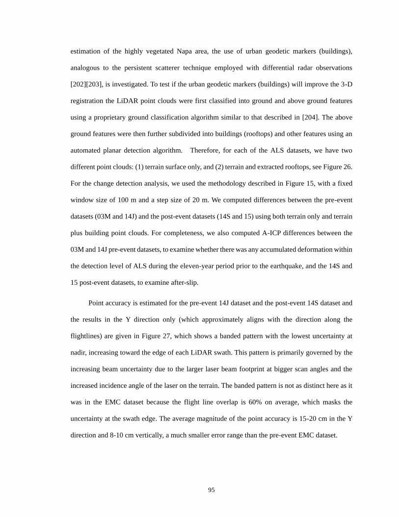
95

estimation of the highly vegetated Napa area, the use of urban geodetic markers (buildings),

analogous to the persistent scatterer technique employed with differential radar observations

[202][203], is investigated. To test if the urban geodetic markers (buildings) will improve the 3-D

registration the LiDAR point clouds were first classified into ground and above ground features

using a proprietary ground classification algorithm similar to that described in [204]. The above

ground features were then further subdivided into buildings (rooftops) and other features using an

automated planar detection algorithm. Therefore, for each of the ALS datasets, we have two

different point clouds: (1) terrain surface only, and (2) terrain and extracted rooftops, see Figure 26.

For the change detection analysis, we used the methodology described in Figure 15, with a fixed

window size of 100 m and a step size of 20 m. We computed differences between the pre-event

datasets (03M and 14J) and the post-event datasets (14S and 15) using both terrain only and terrain

plus building point clouds. For completeness, we also computed A-ICP differences between the

03M and 14J pre-event datasets, to examine whether there was any accumulated deformation within

the detection level of ALS during the eleven-year period prior to the earthquake, and the 14S and

15 post-event datasets, to examine after-slip.

Point accuracy is estimated for the pre-event 14J dataset and the post-event 14S dataset and

the results in the Y direction only (which approximately aligns with the direction along the

flightlines) are given in Figure 27, which shows a banded pattern with the lowest uncertainty at

nadir, increasing toward the edge of each LiDAR swath. This pattern is primarily governed by the

increasing beam uncertainty due to the larger laser beam footprint at bigger scan angles and the

increased incidence angle of the laser on the terrain. The banded pattern is not as distinct here as it

was in the EMC dataset because the flight line overlap is 60% on average, which masks the

uncertainty at the swath edge. The average magnitude of the point accuracy is 15-20 cm in the Y

direction and 8-10 cm vertically, a much smaller error range than the pre-event EMC dataset.

96

Figure 27 Point accuracy in Y (cm) for the 14J (left) and 14S (right) Napa earthquake datasets. Boxes

on the Y accuracy plot estimate flight line extents for the pre-event LiDAR dataset.

5.2.3 Results and Discussion

The results of the moving window A-ICP estimate of coseismic and postseismic deformation

associated with the South Napa earthquake are given in the following sections. The improvements

using the multi-return and classified point cloud as geodetic markers on the performance of moving

window A-ICP for near-fault displacement estimations is also discussed. The differential results

are compared with field measurements to discuss the uncertainty of the moving window A-ICP

algorithms.

5.2.3.1 Seismic Slip

The results of seismic changes between 14J and 14S in the terrain only data and the terrain

plus geodetic marker data are presented in Figure 28 (Napa area) and Figure 29 (Brown’s Valley

area), together with the two primary fault traces, the one in the west in red and the east in black,

estimated from field observations of surface offsets as a reference. The fault trace in black showed

97

only minimal surface displacements of a few cm [199], which is below the threshold of detection

for ALS; no discernible pattern near this fault trace is evident.

The temporal difference between 14J and 03M in Figure 30 was examined to look for pre-

seismic creep present along the west Napa fault. Two primary fault traces (the one on the west in

red and the east in black) overlaid on the A-ICP results are estimated from connecting field

observations of surface offsets as a reference. Fault creep is defined as the slow rupture of the

earth’s crust, which offsets and deforms curbs and streets but make little impact on the rooftops of

buildings and other structures that sit on top of the fault. Note that the differential results of terrain

only and terrain with geodetic markers shows an average close to zero, with a large spread of noise

~19 cm and no evident deformation pattern across the Napa area. By block modeling of GNSS data,

a slip rate of 4.0 ± 3.0 mm/yr was estimated along the west Napa fault [205], which agrees with the

mean offset of ~2 cm estimated by differencing ALS between 14J and 03M. However a flat pre-

earthquake of zero offset was observed from Plate Boundary Observatory site P261 near this fault

before the Napa earthquake [34], and without other published data from permanent geodetic

stations along this fault showing validated pre-earthquake near- fault displacement, the

displacement seen between 14J and 03M should not be definitively interpreted as a fault creep

signal.

Box plots of estimated deformation for 14S minus 14J are shown in Figure 31. The results

for Brown’s Valley are shaded in light blue and results for the entire Napa extents are shaded in

deeper blue for comparison. The box plots of terrain only change are shown in blue and the boxplots

of terrain with geodetic markers are shown in black. The bars inside the boxes represent the median

value of the estimated displacement in each scenario. The rectangles represent the middle half of

the data, showing the 25th to 75th percentile range. The lines, or error bars, go from the minimum

to the maximum values.

98

Figure 28 A-ICP results of Napa area for 14S minus 14J. From top to bottom: change of terrain only and

the terrain and geodetic markers. From left to right: estimated displacements in X, Y and Z

directions.

The estimated change between the 14J and 14S datasets, taken right before and after the

earthquake, is presented in Figure 28 and shows markedly good segregation of the surface

displacement, especially in Y direction that is approximately parallel with the fault line. The results

in Figure 31 indicate that the estimated change is significant within the range of the estimated

displacement accuracy. The results of terrain with geodetic markers do not show significant

improvement compared to using terrain only. However, when examining the hill shade in Figure

26, it is observed that the majority of the buildings are restricted to one subdivision – Brown’s

valley, outlined with a yellow rectangle. This observation suggests that change in building rooftops

can be hidden in the statistics because the majority of the area has no buildings and, therefore, the

99

moving window scheme results in buildings only being present in a few windows. Therefore, to

further investigate the performance of the addition of geodetic markers, change detection for only

the Brown’s Valley neighborhood is presented in Figure 29 with two primary fault traces (the one

on the west in red and the east in black) overlaid on A-ICP result are estimated from connecting

field observations of surface offsets as a reference, and boxplots are given in Figure 31.

Figure 29 A-ICP results of displacements of Brown’s Valley for 14S minus 14J in X, Y and Z directions.

From top to bottom: change of terrain only, the histogram with mean and standard deviation

(cm) of estimated terrain only displacement on each side of the west fault line (red), change

of terrain and geodetic markers, and its histogram of displacement estimated.

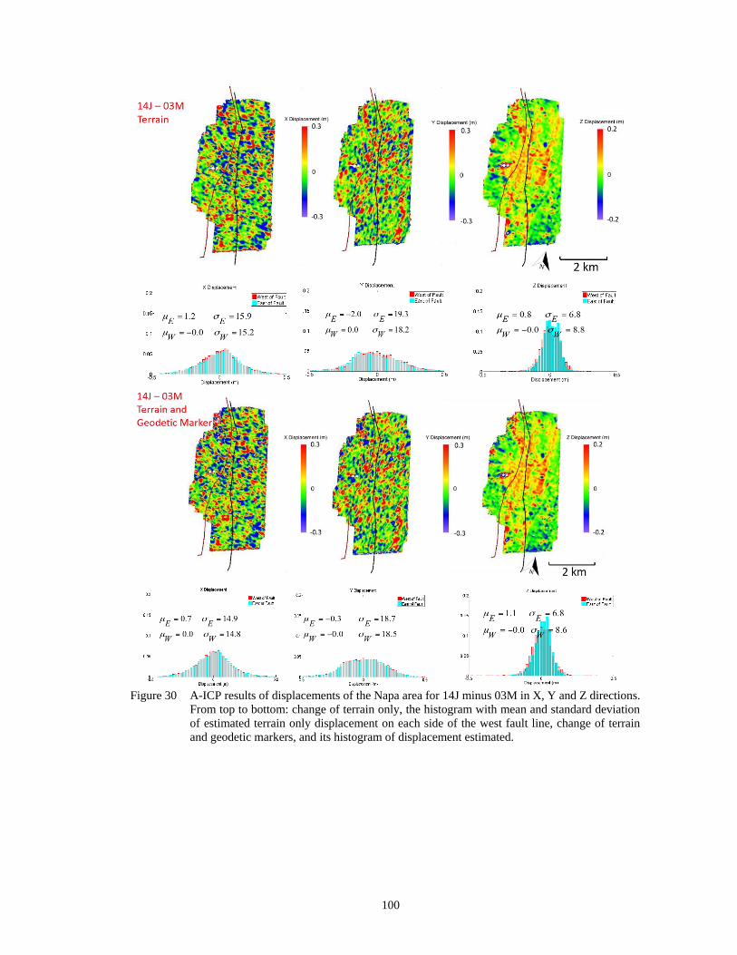
100

Figure 30 A-ICP results of displacements of the Napa area for 14J minus 03M in X, Y and Z directions.

From top to bottom: change of terrain only, the histogram with mean and standard deviation

of estimated terrain only displacement on each side of the west fault line, change of terrain

and geodetic markers, and its histogram of displacement estimated.

101

Figure 31 Box plots of deformation estimated for 14S minus 14J. The results for Brown’s Valley are

shaded in light blue (left) and results for Napa area are shaded in deeper blue (right) for

comparison. The box plots of terrain only change are in blue and terrain and geodetic marker

boxplots are in black.

A close examination of the displacement maps provided in Figure 29 clearly show that the

addition of geodetic markers improves the estimation by moving window A-ICP. The surface

rupture is delineated clearly, the noise level is reduced, and the standard deviation of horizontal

displacement is reduced to under 10 cm, and under 3 cm for the vertical displacement, a much

smaller value than that of the results for the entire Napa area (Figure 28). Although some houses

may have undergone change during the period after the earthquake, the majority of the structures

are expected to be unchanged. Therefore, the urban geodetic markers can be used as control points

for persistent scatter and the accuracy of moving window A-ICP with the augmentation of geodetic

markers significantly improves the A-ICP results.

5.2.3.2 Postseismic and After-slip

The results of seismic, postseismic, and after-slip change of terrain only and terrain plus

geodetic markers between 14J and 15 are presented in Figure 32, for all of the Napa area and Figure

33 for only the Brown’s Valley neighborhood. Two primary fault traces, the one on the west in red

and the east in black, estimated from field observations of surface offsets, are also shown as a

102

reference. The results of postseismic and after-slip change of terrain only and terrain plus geodetic

markers between 14S and 15 are presented in Figure 33 for all of the Napa area and Figure 35 for

only the Brown’s Valley neighborhood. Two primary fault traces (the one on the west in red and

the east in black) overlaid on A-ICP results are estimated from connecting field observations of

surface offsets as a reference.

Box plots of estimated deformation are shown in Figure 36 for 14J and 15 and in Figure 37

for 14S and 15. The results for Brown’s Valley are shaded in light blue and results for all of the

Napa area are shaded in deeper blue for comparison. The box plots of terrain only change are in

blue and the results of terrain with geodetic markers are in black. The bars inside the boxes represent

the median value of the estimated displacement of each scenario. The rectangles represent the

middle half of the data, from the 25th to the 75th percentile. The lines, or error bars, range from the

minimum to the maximum values.

By comparing the A-ICP results of all of the Napa area in Figure 28 (14S minus 14J) and

Figure 32 (15 minus 14J), the 15 minus 14J results are in agreement with 14S minus 14J. The

differences between these two are within the expected noise level of the ALS point clouds. The

estimated results for 14S minus 15 for the Napa area displayed in Figure 33. The median and data

spread of 15 minus 14S within Brown’s Valley indicates an agreement with the field observations

of the alignment array which showed a small amount of accumulated after-slip on this portion of

the fault. As an example, Leaning Oak Drive (NLOD) USGS alignment array site located at the

south end of Brown’s Valley neighborhood [199] has seen 40 mm of slip between 5 and 60 days

following the South Napa earthquake, assuming the datum of these observations is correctly

accounted. However, the estimated movements of 15 minus 14S are all within noise level of the A-

ICP approach, therefore uncertainty must be carefully analyzed before any interpretation of

discernable pattern of postseismic or after-slip movement. The analysis of the accuracy of the A-

ICP approach will be discussed further in the next section.

103

Figure 32 A-ICP results of displacements of Napa area for 15 minus 14J in the X, Y, and Z directions.

From top to bottom: change of terrain only and terrain with geodetic markers.

A close–up examination of the A-ICP results for the Brown’s valley area, 15-14J, where more

rooftop features are present closer to the locations of the fault traces, is shown in Figure 33. There

is a more discernible displacement in the Y direction to each side of the fault line. Results in the Y

direction show movement of ~25 cm (to the south) east of fault line between 15 and 14J, while

movement between 14J and 14S (Figure 29) is ~20 cm. Results are much cleaner in this area than

in the extended area and have a very low standard deviation of ~2 cm in the vertical direction.

104

Figure 33 A-ICP results of displacements of Napa area for 15 minus 14S in the X, Y, and Z directions.

From top to bottom: change of terrain only and terrain with geodetic markers.

Figure 34 A-ICP results of displacements of Brown’s Valley for 15 minus 14J in the X, Y, and Z

directions. From top to bottom: change of terrain only and terrain with geodetic markers.

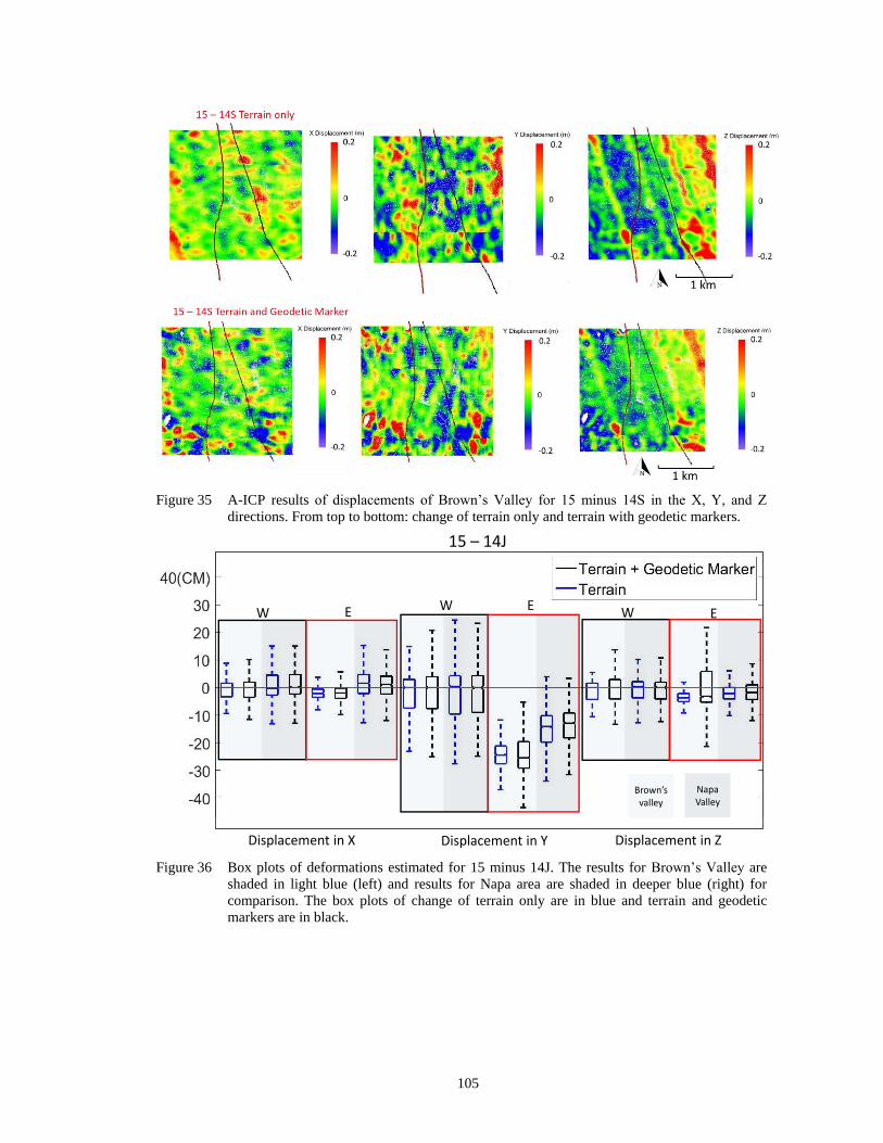
105

Figure 35 A-ICP results of displacements of Brown’s Valley for 15 minus 14S in the X, Y, and Z

directions. From top to bottom: change of terrain only and terrain with geodetic markers.

Figure 36 Box plots of deformations estimated for 15 minus 14J. The results for Brown’s Valley are


comparison. The box plots of change of terrain only are in blue and terrain and geodetic

markers are in black.

EWEW

EW

Brown’s valley

Napa Valley

15 – 14J

Displacement in X Displacement in Y Displacement in Z

106

Figure 37 Box plots of deformations estimated for 15 minus 14S. The results for Brown’s Valley are


comparison. The box plots of change of terrain only are in blue and terrain and geodetic

markers are in black.

Box plots of the A-ICP estimated deformations for the entire NAPA extents in the X, Y, and

Z directions are shown in Figure 38. An overview of the results for 14J minus 03M, 14S minus 14J,

15 minus 14S, and 15 minus 14J are given respectively. The box plots showing the change in terrain

only are in blue and the boxplots showing the terrain with geodetic markers are in black. The results

to the east of the major fault line are shaded in yellow and those to the west are shaded in pink. The

primary movement observed is on the west side of the major fault line in the Y direction, which

confirms to the field observation that the movement during the Napa earthquake was primarily right

lateral slip. The boxplots show the statistical agreement of the 15 minus 14J results with the 14S

minus 14J results, with 15 minus 14J containing the effect of noise observed in the results of 15

minus 14S. The results from each set of differential datasets are within the noise level of the A-ICP

approach and the expected accuracy of the LiDAR point clouds, demonstrating the accuracy of the

A-ICP application in the estimation of seismic movement. The statistics from terrain with geodetic

markers are comparable to those with terrain alone; though the terrain with geodetic marker results

show slightly more segregation of the surface displacement between each side of the fault line. The

EWEW

EW

Brown’s valley

Napa Valley

15 – 14S

Displacement in X Displacement in Y Displacement in Z

107

differential results also display repeatability of the moving window A-ICP approach for near-fault

deformation estimates.

Figure 38 From top to bottom, the box plots of deformations for the entire Napa extents decomposed in

the X, Y, and Z directions. Statistics of results for 14J minus 03M, 14S minus 14J, 15 minus

14J, and 15 minus 14J are given respectively.

108

5.2.3.3 Discussion of Accuracy

Similar to the EMC earthquake, in-situ surface rupture observations that record the

orientation, length, and direction of the fault slip were useful in the aftermath of the Napa

earthquake and provided valuable first hand documentation, sometimes within a few hours of the

event. In order to compare the field observations to the moving window A-ICP result for 14S minus

14J and to validate the accuracy of the A-ICP application, moving window A-ICP was executed

over an extended area that covers the entire overlapping part of both datasets, including as many

field measurement locations as possible. The locations of field measurements agree well with

schematic rupture traces of linear features indicated by a difference in elevation that is estimated

with A-ICP. Therefore, profiles with a center pinned on every field measurement site were drawn

from the A-ICP result. The field measurements are compiled from [206] and [34] and are shown as

black dots on Figure 39. The orientation and kinematics of each fault section are presented in these

studies, unfortunately the measurements are only of the total displacement and no separation of

horizontal and vertical components was available. Black dots in Figure 39 indicate the locations of

in-field hand measurements. The black line is a connected polyline representing the estimated fault

line locations; there is one major fault line in the West and a more subtle one in the east. The color

shows the amount of movement in the Y direction (m) estimated by moving window A-ICP.

A comparison between the field measurements and the A-ICP results, interpolated to the

same locations, was performed. The results are shown in Figure 40. Uncertainties for LiDAR point

cloud collection and A-ICP registration are shown as shaded areas in the figure in blue and pink,

respectively, and will be used as a bracket threshold to detect outliers. For comparison, the results

of tile wise ICP and moving window ICP are also interpolated to the locations of field measurement,

and shown in the same Figure 40. The field measurements only provide total displacement, as

separate horizontal and vertical displacements were not recorded.

109

Figure 39 Transect profiles overlay on A-ICP results for 14S minus 14J. The colored estimated

displacements are change of terrain only displacements in the Y direction.

Figure 40 Horizontal offsets between ALS differential estimates using 14S minus 14J and field

measurements, marked by circle (tile wise ICP), asterisk (moving window ICP), and diamond

(moving window A-ICP), at corresponding distance between the ICP window center and

locations of field measurements (2014 August) along the rupture trace.

110

The original 12 field data points were examined using photographs and geographic locations

of the field measurements and, from these, 9 points were used for ground truth reference. The

horizontal displacement differences for excluded points 4, 8, and 9 are much larger than the mean

estimated accuracy of the A-ICP results. Figure 39 shows the locations of the point excluded. Point

8 had the largest displacement, ~46 cm, recorded from field measurements, and there is a clear

discrepancy between the estimate from A-ICP and the point taken. However, closely examining the

results in the area around point 8, there is an area of offset of 40-50 cm as shown in Figure 28.

Although point 8 is taken out of the calculation, the A-ICP estimates of the surrounding area match

well with the field measurement of point 8. A potential source of error might come from the soft

sediments surrounding the field measurement area [199], which could degrade the accuracy of field

measurements. Photographs of the surrounding environment of the field measurement of point 8 is

shown in Figure 41. However, with the high spatial density of the ALS differential results, the

discrepancy at a single point does not substantially impact the estimated near-field deformation.

Point 4 and point 9 have a similar situation with point 8, although large offsets are present in the

direct comparison, a good agreement can be observed in the surrounding area.

The statistics of tile wise ICP, moving window ICP, and moving window A-ICP results are

presented in Table 7. Tile wise ICP shows the largest differences, which is likely due to the limited

spatial resolution of the tile-wise ICP because a positive correlation can be observed between the

discrepancies between tile wise ICP and the field measurements and the distance from the ICP

window center to the field measurement locations (Figure 40). Moving window ICP slightly

improves the agreement between the differential estimates and the field measurements, but not as

good as moving window A-ICP. This observation applies to both the case of 15 minus 14J and 14S

minus 14J. This once again confirms that the anisotropic estimates of point uncertainty provide a

clear improvement in ALS estimated near-field deformation.

111

Table 7 The statistics of differences between ALS differential estimates using tile wise ICP, moving

window ICP, and moving window A-ICP and field measurements of the Napa earthquake for

both 14S minus 14J and 15 minus 14J.

Figure 41 Photographs showing a characteristic of right-lateral fault displacement at the ground surface

features resulting from fault displacement during the Napa earthquake. Right-lateral

displacement of 40 cm was measured near this location one day after the earthquake.

Photograph by Dan Ponti, USGS [199].

Near-fault displacements and fault scarp localization agree well with field measurements at

the sub-decimeter scale but also reveal some local metric discrepancies. The statistical results, after

the removal of the three outliers, show a fair agreement with field measurements, demonstrating

Datasets Differential Method Mean (m) Standard Deviation (m) RMSE (m)

14S minus 14J Tile wise ICP 0.147 0.182 0.234

Moving window ICP 0.041 0.145 0.151

Moving window A-ICP -0.032 0.105 0.110

15 minus 14J Tile wise ICP 0.054 0.201 0.208

Moving window ICP -0.004 0.120 0.121

Moving window A-ICP 0.039 0.113 0.120

112

the value of weighting the ALS data using point accuracy in 3-D differencing. The shaded blue area

is larger than the pink area overall (Figure 40), consistent with the relationship of mean error of the

A-ICP estimation and the mean error of LiDAR point accuracy. This suggests that the offsets

generally agree with localized measurements in the field.

An independent samples t-test was conducted for the 14S minus 14J results, in order to

compare the differences between the moving window A-ICP estimates and the field measurements

versus the differences between the tile wise ICP estimates and the field measurements. The

variances in the horizontal differences were significant between moving window A-ICP (mean=-

0.032m, RMSE=0.110) and tile wise ICP (mean=-0.147m, RMSE = 0.234m); t (18) = 2.5490, p =

0.0201. These results suggest that moving window A-ICP has significantly better horizontal

agreement with the field measurements.

An independent samples t-test was also conducted to compare the differences between the

moving window ICP estimates and the field measurements versus the differences between the tile

wise ICP estimates and the field measurements. There was not a significant variance in the

horizontal differences between moving window ICP (mean = 0.041m, RMSE = 0.151m) and tile

wise ICP (mean = 0.147m, RMSE = 0.234) and; t (18) = 1.3628, p = 0.1897.

These results suggest that moving window ICP does not show a significantly better horizontal

agreement with the field measurements when compared to tile wise ICP. While the moving window

technique was able to provide marginal improvement in the agreement with the field measurements,

it is clear that the anistropic uncertainty estimates provide the largest improvement in the estimate

of near-field displacement. The results of the independent samples t-test for 15 minus 14J shows

similar results. This also agrees with the results in the previous section for the EMC earthquake

The RMSE of the horizontal offsets is ~11cm for 14S minus 14J and ~12 cm for 15 minus

14J (Table 7). One point to be noted is that the field observations are collected with a tape measure

and generally measured as piercing-line offsets and recorded with an azimuth along which the

113

measurement was made (see pictures in [207][206]). Although the field measurements were

delivered as total displacement, they most likely represent horizontal displacement alone. The

slightly larger than expected size of the differences may be caused by vertical displacements in the

measured total field displacement, which were not included in the A-ICP displacement estimates.

Although the vertical movement during the Napa Earthquake was not pronounced in the A-ICP

results there may be local vertical displacements along offset features that appeared in the field

measurements of total displacement. However, the magnitude and orientation of this error is

difficult to quantify.

6 CONCLUSIONS AND FUTURE WORK

6.1 Contributions of Dissertation and Conclusions

In this dissertation, we have examined the ability of ALS to recover locally varying surface

displacements over large spatial scales and studied a potentially optimal method for estimating and

representing the deformation.

First, the current LiDAR–based change detection methods were introduced, including

algorithms ranging from 1-D to 2-D to state-of-the-art 3-D registration methods. The performance

of 3-D change detection methods, including closest point criterion based (i.e., ICP) method and its

variants suitable for surface deformation and probability based 3-D registration (CPD) for both

rigid and non-rigid systems, were then evaluated experimentally. The convergence behavior,

computation time, and matching accuracy of every method was assessed in terms of the stability

and robustness of transformation, noise level, and sample rate. Overall, in the case of a locally

varying density dataset that is similar to a real ALS scanning scenario, point to point ICP shows the

best overall performance. Point to point ICP had the lowest computing time and average GMA

throughout the tests when measured against varying shift amounts, sample rates, and noise levels.

114

Next, point to point ICP was closely examined to determine the optimal scheme and

parameters used to autonomously estimate spatially varying earthquake caused 3-D displacements.

A new variant of the ICP algorithm, A-ICP, which incorporates the point accuracy estimation, was

developed to overcome the difficulties associated with sparse legacy pre-event datasets. It has been

shown that A-ICP can both speed up the ICP process and improve the matching accuracy. In

addition, a new “moving window” partition scheme was proposed to handle the large spatial scale

point cloud over an earthquake-influenced area and to enhance the change detection results for local

varying surface deformation in the near-fault region.

Two real world case studies of actual earthquakes were presented in this research to analyze

the potential of repeat ALS surveys to recover near-fault displacements using the optimal

parameters for ICP methods. While other studies have examined LiDAR-based earthquake

introduced surface displacements with repeat ALS surveys of similar point density, to date no work

has been done to address the difficulties presented when there is a large point density disparity

between pre- and post-event datasets. The first case study, of the EMC earthquake, included a post-

event dataset 1000 times as dense as the pre-event dataset. Moving window A-ICP clearly

delineated the surface rupture in the profiles across the fault line in all three components of

displacement. Less noise and more detail is observed from the moving window A-ICP, when

compared to standard ICP, and it appears to perform better for overcoming the banded error pattern

caused by increased uncertainty at the edge of the pre-event ALS swaths. A comparison of ALS

differential results with field observations of deformation estimated using offset features along the

documented surface rupture was also made. The mean values of differences between the moving

window A-ICP estimates and the field measurements are near zero for both the horizontal and

vertical displacements, while the tile-wise and moving window ICP both have offsets in the

horizontal direction of ~0.6 m. The RMSE of the moving window A-ICP vertical differences is

0.464 m and the RMSE of the horizontal differences is 0.648 m. The ratio of the vertical and

115

horizontal differences is consistent with the mean error of the pre-event A-ICP estimation as well

as the mean error of LiDAR point accuracy, suggesting that the offsets generally agree with

localized measurements in the field. Overall, the moving window A-ICP results have a better

agreement with field measurements than the tile wise ICP and the moving window ICP,

demonstrating the value of weighting the pre-event data using point accuracy in arid rural areas.

The results of the comparison validated the sub-meter level accuracy of the ALS differential.

Results of applying moving window A-ICP to pre- and post-event EMC datasets show that

both the ER of the last iteration and the difference between A-ICP and ICP vertical displacement

estimates mirror the estimated pre-event LiDAR point accuracy as evidenced by the striped pattern

Figure 21 (a) (b). The same pattern is observed in change detection results for the South Napa

earthquake, which aligns with the flight line stitching pattern. However, this pattern is mitigated by

incorporating LiDAR point accuracy into the A-ICP algorithm. The ability of A-ICP to overcome

this problem, by making use of point accuracy as an anisotropic weighting factor, is rigorously

estimated and the error estimation is modelled to provide the accuracy of the A-ICP algorithm and

assist in removing outliers during ground measurement validation.

While the EMC earthquake study represents a coarser LiDAR point cloud collection and

larger magnitude earthquake displacement, the Napa earthquake study shows the potential of ALS

differencing to reveal smaller surface displacements. It provides more detailed insight into the

magnitude of surface displacement that can be recovered with high resolution ALS datasets. For

Napa, the estimated surface displacements are at or near the sample interval and estimated accuracy

of the ALS observations. In this case, the results from the South Napa earthquake registration and

change detection indicate that the use of urban geodetic markers as persistent scatterers can

significantly improve estimates of coseismic and postseismic displacement in built-up areas. The

seismic slip estimation in the Y direction to each side of the fault line shows average movement of

~20 cm (to the south) on the east side of the fault. The standard deviation of the horizontal

116

displacement is noticeably reduced to under 10 cm, from ~15 cm, and the standard deviation of the

vertical displacement is reduced to ~3 cm, from ~7 cm.

The 15 minus 14J results are in agreement with the 14S minus 14J results for the entirety of

the Napa Valley point cloud collections. The differences between these two are within the expected

noise level of the ALS point clouds. The median of the estimated postseismic movement in the Y

direction, based on 15 minus 14S, within Brown’s Valley, is ~3 cm to the south with a standard

deviation of 4.5 cm. However, this possible postseismic contribution is still within the noise level

of the A-ICP approach; therefore, uncertainty is discussed and analyzed and the results of the A-

ICP estimates are compared to field observations for verification. The field observations from the

alignment array site, NLOD, located at the south end of the Brown’s Valley neighborhood, also

showed an accumulated after-slip of 4 cm on this portion of the fault between 5 and 60 days

following the South Napa earthquake.

A comparison was made between the ALS based near-field deformation from the South Napa

earthquake over an extended area with both temporal and spatial 3-D changes and the field

observations of deformation, which were estimated using offset features along the documented

surface rupture. The results of the comparison confirmed the decimeter level accuracy of the ALS

differential results. The statistics of the offset between the results of tile wise ICP and moving

window ICP were also presented. Tile wise ICP shows the largest deviations, with a mean

horizontal offset of 14.7 cm and a RMSE of 23.4 cm, which is likely due to the spatial limitation

of the tile-wise ICP. A moving window A-ICP approach overcomes the spatial limitation and the

weighting scheme improves the agreement between field measurements and ICP so that the mean

horizontal offset is near zero with a RMSE of ~11 cm.

Near-fault displacements and fault scarp localization based on moving window A-ICP agree

at the sub-decimeter scale with field measurements for the Napa earthquake and at the sub-meter

scale for the EMC earthquake. The statistical results of the A-ICP approach, after the removal of

117

the outliers, show a fair agreement with field measurements and outperform the standard tile wise

ICP and moving window ICP, demonstrating the value of weighting the ALS data using estimated

point accuracy. The ratio of vertical and horizontal differences between A-ICP estimates and field

measurements are consistent with the mean error of the A-ICP estimation as well as the mean

estimated error of the LiDAR points.

These observations of surface displacement, including both the coseismic surface

displacement field and early postseismic deformation, are commonly used to map the fault location

and static slip distribution (SD) of earthquakes and to assess associated static stress changes on

neighboring faults. In addition to exploring the source properties of earthquakes, the importance of

rapidly updated geodetic observations, both in situ and remotely sensed, for event source

characterization and response, lays in their applicability to geodetic-based finite-fault inversions

[208]. Where available, geodetic observations complement these finite source models, providing

additional constraints on slip location and complexity and expanding on composition and rheology

that are essential to characterize the crustal structure in relation to the geology and tectonic

evolution of the region. Events, like the South Napa earthquake, demonstrate the utility of geodetic

observations in constraining slip complexity and the resulting stress changes from small to

moderate magnitude earthquakes. Before LiDAR differential applications, the inversion was done

by jointly inverting the GPS and down-sampled InSAR observations for the location, orientation,

and dimensions of a single-fault patch with homogeneous slip embedded in a homogeneous elastic

half-space using the neighborhood algorithm [208] [209]. However, this approach often fails to

obtain unique solutions using these spatially oversampled data, or it fails to hold the homogeneous

assumptions when dealing with data that show complicated site responses but lack near-fault details.

Therefore, as a part of the response to the earthquake, geodetic data with higher sampling density

and spatial coverage closer to the fault should be progressively incorporated into the inversion

models.

118

The results of this inversion modeling based on the neighborhood algorithm show the results

of a spatially limited data source. The resolution of the distributed slip can be seen by using an

iterative method in which the fault is discretized with variably sized triangles that reflect the model

resolution afforded by the surface observations (Figure 42). The uncertainty in the SDs, caused by

sparse data and represented by large triangles, can be dramatically decreased using the

incorporation of high spatial resolution near-fault data, like that collected in ALS studies.

Figure 42 Median value finite slip distributions (SDs) derived from Monte Carlo analysis for the Napa

Valley Earthquake. (a, b) Plan and map view of the east-dipping focal plane (strike 341°, dip

80°) with observed (black) and modeled (red) continuous Global Positioning System (GPS)

displacements [208].

Using low spatial resolution source geodetic data to inform inversion models leads to biased

modeled results. The lack of surface deformation data near-fault leaves the model unable to

conclusively determine the geometry of the fault surface that slipped during an earthquake.

Spatially dense observations from a single interferogram or optical image-differencing approach

may also be insufficient to constrain the characteristics of an earthquake to the degree needed for

products like ShakeMap. The LiDAR differential methods used in this study may serve as a

template for future earthquakes when pre- and post-earthquake LiDAR data are available and can

be incorporated into geomechanical modeling.

Using an inverse model, it is possible to use the LiDAR based 3-D deformation mapping to

solve for a distribution of slip along a predefined fault geometry. Earthquake movement magnitudes

can be computed from the fault slip distributions by first computing the seismic moment tensor and

119

the scalar seismic moment [210]. Using a slip solution the model can be forwarded to predict

displacement, which can be compared with the regional surface observations [199], [211].

Statistically, the significant improvement in accuracy from the use of moving window A-ICP,

compared to the commonly used tile wise ICP, will improve the model of SDs, the earthquake

movement characterization, and, in turn, the predicted displacements. The spatial resolution of

input estimated displacement is improved from kilometer level to decimeter level, and the accuracy

of these is as high as the accuracy of the LiDAR collection. The information that is sought will

eventually be obtained from the observations using inversion models of earthquake physics,

therefore both spatial resolution and accuracy of improvement contributes to the accuracy

improvements in the inversion models.

6.2 Future Work

In this dissertaion, various areas were identified where further research was needed.

Recommendations for future work include the following two major areas: (1) improving the ALS

differencing techniques, and (2) the integration of near-field ALS displacements into inversion

models for earthquake physics.

6.2.1 Improved ALS Differencing Techniques

Highly accurate details regarding near-fault displacements can be achieved by differencing

repeat LiDAR surveys along fault lines, as shown in this work and work done by others. These

results have provided further motivation to expand the range of active faults mapped with LiDAR

and the research focus of 3-D differencing techniques.

120

6.2.1.1 Expanding LiDAR Differencing of Active Faults

The recent increase in airborne LiDAR data collections along active faults in the western

United States will provide a baseline for future earthquake displacement studies. These

displacements will help constrain the slip distribution and rheology of the shallow part of the fault

zone, which are both crucial for interpreting seismic movements and long-term earthquake behavior.

These improvements are not limited to airborne LiDAR applications. The increased availability of

current and future space based LiDAR data from ICESat GLAS, ICESat-II/GLAS, and DESDynI/

LiDAR will create a global network of LiDAR transects covering a variety of terrain types. Based

on these data, a global project can be built for earthquake deformations using the 3-D differential

– based change detection techniques presented here.

6.2.1.2 Error Analysis of Legacy LiDAR Data

Many legacy LiDAR datasets exhibit residual systematic errors. It is important for future

differencing work, which will rely on such legacy data, to perform error analysis that combines

errors from GNSS positioning, trajectory, ranging, and scanning mechanisms, if the original raw

observations can be obtained. Rigorous error estimation to examine the ALS differencing accuracy

is also recommended for future work. A weighting strategy using the point accuracy of LiDAR

point clouds is introduced in this dissertation, to partially overcome the impact of striped error

pattern found in older ALS results. Investigating ways to improve the algorithm efficiency and

effectiveness by making use of point accuracy estimation in the LiDAR point cloud would be a step

forward in the field of LiDAR – based change detection.

6.2.1.3 Extending the Research of 3-D Differential Techniques

Further research into the applications of 3-D differential methods to determine earthquake

deformation would be beneficial to the earth sciences, given the abundance of information ALS 3-

121

D differentials can provide. The proposed CPC-based algorithm primarily takes into account the 3-

D positions and some prior parameters (point accuracy and classification of point cloud) in order

to align two point clouds and detect change. Limitations on the existing algorithms have been

discussed at length in Chapter 3 and it was shown that such information might not be always

available. In future studies, the focus on the generalization of ICP, further advancement of the ICP-

like methods, and the improvement of probability-based 3-D registration methods, such as CPD,

for applications such as earthquake deformation should be expanded. In this dissertation, the

addition of geodetic markers has demonstrated improvement to the ALS differencing results. For

future advancement of 3-D differencing techniques, the inclusion of other geodetic markers, such

as stable geometrical features, should be studied.

6.2.2 Integration of ALS with Other Observations in Earthquake Physics

ALS provides a wealth of near-fault displacement data to complement existing geodetic or

field-based observations. InSAR and sub-pixel optical matching can map earthquake deformations

with high precision over wide areas. However, they fall short of providing full 3-D surface

displacements and also suffer from coverage gaps close to the surface faulting. The employment of

ALS differencing has proven to provide near-fault deformation with significant details and accuracy,

but has been limited by data coverage up to now. However, when coupled with satellite-based

measurements, including InSAR and optical imageries, differential LiDAR will also offer the

means to explore relations between surface rupturing and deeper fault zone processes. The

integration can be realized with multi-sensor integrated systems. These systems can be operated in

periodic mode, with repeated operator surveys, and quality controlled by deploying permanent

GNSS receivers. The most difficult parts of the design will be the hardware configuration for the

monitoring network and the georeferencing and calibration among the native reference frames

adopted by each instrument.

122

The integration can also be realized by data fusion or the generation of a common earth

science model. A practical realization would be the extraction of a common 3-D model, such as a

deformation image, to represent the combined terrain information of each respective instrument,

including far-field InSAR estimates, long term and temporary GNSS observations and optical

imagery, together with LiDAR. By integrating other data sources, the accuracy of the deformation

image for monitoring the subtle ground surface deformation induced by natural hazards will be

improved. A cohesive model will also clarify the kinematics of the earthquake movements and

facilitate simulations of the most probable structural behavior of the monitored earth surfaces.

Finally, LiDAR based 3-D change detection and the integration of LiDAR displacements

with other observations should not be limited to earthquake applications, but be used in a larger

range of geomorphology studies such as the dynamics of ice sheets during deglaciation, the volume

calculation of landslide features, and shoreline displacement monitoring.

123

REFERENCES

[1] L. Pakiser and K. M. Shedlock, Earthquakes (Illustrations): 2014.

[2] B. Stevens and S. E. Schwartz, “Observing and Modeling Earth’s Energy Flows,” Surv. Geophys.,

vol. 33, no. February, pp. 779–816, 2012.

[3] R. H. Sibson, “Earthquake Faulting as a Structural Process,” Journal of Structural Geology, vol. 11,

no. 1–2. pp. 1–14, 1989.

[4] D. W. Forsyth, T. Lay, R. Aster, and B. Romanowicz, “Grand Challenges for Seismology,” Eos

Trans. AGU, vol. 90, no. 41, pp. 361–362, 2009.

[5] G. Rogers and H. Dragert, “Episodic Tremor and Slip on the Cascadia Subduction Zone: The Chatter

of Silent Slip.,” Science, vol. 300, no. 5627, pp. 1942–1943, 2003.

[6] A. Pitarka, K. Irikura, T. Iwata, and H. Sekiguchi, “Three-Dimensional Simulation of the near-Fault

Ground Motion for the 1995 Hyogo-Ken Nanbu (Kobe), Japan, Earthquake,” Bull. Seismol. Soc.

Am., vol. 88, no. 2, pp. 428–440, 1998.

[7] E. Nissen, A. K. Krishnan, J. R. Arrowsmith, and S. Saripalli, “Three-Dimensional Surface

Displacements and Rotations from Differencing Pre- and Post-Earthquake LiDAR Point Clouds,”

Geophys. Res. Lett., vol. 39, no. 16, Aug. 2012.

[8] J. F. Dolan and B. D. Haravitch, “How Well Do Surface Slip Measurements Track Slip at Depth in

Large Strike-Slip Earthquakes? The Importance of Fault Structural Maturity in Controlling on-Fault

Slip versus off-Fault Surface Deformation,” Earth Planet. Sci. Lett., vol. 388, no. C, pp. 38–47, Feb.

2014.

[9] P. G. Somerville, “Magnitude Scaling of the near Fault Rupture Directivity Pulse,” Phys. Earth

Planet. Inter., vol. 137, no. 1–4, pp. 201–212, 2003.

[10] R. McCaffrey, “The next Great Earthquake,” Science (80-. )., vol. 315, no. 5819, pp. 1675–1676,

2007.

124

[11] J. Jackson, “Living with Earthquakes: Know Your Faults,” J. Earthq. Eng., vol. 5, no. 1, pp. 5–123,

2001.

[12] F. F. Pollitz, R. S. Stein, V. Sevilgen, and R. Bürgmann, “The 11 April 2012 East Indian Ocean

Earthquake Triggered Large Aftershocks Worldwide,” Nature, vol. 490, no. 7419, pp. 250–253,

2012.

[13] C. L. Glennie, A. Hinojosa-Corona, E. Nissen, A. Kusari, M. E. Oskin, J. R. Arrowsmith, and A.

Borsa, “Optimization of Legacy Lidar Data Sets for Measuring near-Field Earthquake

Displacements,” Geophys. Res. Lett., vol. 41, no. 10, pp. 3494–3501, 2014.

[14] J. Rice and M. Cocco, “Seismic Fault Rheology and Earthquake Dynamics,” Tecton. Faults Agents

Chang. a Dyn. Earth, vol. 107, pp. 99–137, 2007.

[15] S. E. Minson, B. A. Brooks, C. L. Glennie, J. R. Murray, J. O. Langbein, S. E. Owen, T. H. Heaton,

R. A. Iannucci, and D. L. Hauser, “Crowdsourced Earthquake Early Warning,” Sci. Adv., vol. 1, no.

3, pp. e1500036–e1500036, Apr. 2015.

[16] K. A. Atrocities and M. S. Hamm, “Book Review,” Pure Appl. Geophys., vol. 167, no. 10, pp. 177–

183, 2003.

[17] R. Bilham, N. Suszek, and S. Pinkney, “California Creepmeters,” Seismol. Res. Lett., vol. 75, no. 4,

pp. 481–492, Jul. 2004.

[18] R. O. Burford and P. W. Harsh, “Slip on the San Andreas Fault in Central California from Alinement

Array Surveys,” Bull. Seismol. Soc. Am., vol. 70, no. 4, pp. 1233–1261, 1980.

[19] K. W. Hudnut, Z. Shen, M. Murray, S. McClusky, R. King, T. Herring, B. Hager, Y. Feng, P. Fang,

a Donnellan, and Y. Bock, “Co-Seismic Displacements of the 1994 Northridge, California,

Earthquake,” Bull. Seismol. Soc. Am., vol. 86, no. 1B, pp. S19–S36, 1996.

[20] E. H. Hearn, “What Can GPS Data Tell Us about the Dynamics of Post-Seismic Deformation?,”

Geophys. J. Int., vol. 155, no. 3, pp. 753–777, 2003.

[21] C. Ji, K. M. Larson, Y. Tan, K. W. Hudnut, and K. Choi, “Slip History of the 2003 San Simeon

Earthquake Constrained by Combining 1-Hz GPS, Strong Motion, and Teleseismic Data,” Geophys.

125

Res. Lett., vol. 31, no. 17, p. L17608, 2004.

[22] K. W. Hudnut, Y. Bock, M. Cline, P. Fang, Y. Feng, J. Freymueller, X. Ge, W. K. Gross, D. Jackson,

M. Kim, N. E. King, J. Langbein, S. C. Larsen, M. Lisowski, Z.-K. Shen, J. Svarc, and J. Zhang,

“Co-Seismic Displacements of the 1992 Landers Earthquake Sequence,” Bull. Seismol. Soc. Am.,

vol. 84, no. 3, pp. 625–645, Jun. 1994.

[23] F. Bleibinhaus, J. A. Hole, T. Ryberg, and G. S. Fuis, “Structure of the California Coast Ranges and

San Andreas Fault at SAFOD from Seismic Waveform Inversion and Reflection Imaging,” J.

Geophys. Res. Solid Earth, vol. 112, pp. 1–15, 2007.

[24] F. Bleibinhaus, R. Lester, and J. Hole, “Applying Waveform Inversion to Wide-Angle Seismic

Surveys,” Tectonophysics, vol. 472, pp. 238–248, 2009.

[25] D. Legrand and B. Delouis, “Determination of the Fault Plane Using a Single near-Field Seismic

Station with a Finite-Dimension Source Model,” Geophys. J. Int., vol. 138, no. 3, pp. 801–808, 1999.

[26] J. J. Lienkaemper, F. S. McFarland, R. W. Simpson, and S. J. Caskey, “Using Surface Creep Rate to

Infer Fraction Locked for Sections of the San Andreas Fault System in Northern California from

Alignment Array and GPS Data,” Bull. Seismol. Soc. Am., vol. 104, no. 6, pp. 3094–3114, Oct. 2014.

[27] S. Custódio, M. T. Page, and R. J. Archuleta, “Constraining Earthquake Source Inversions with GPS

Data: 2. A Two-Step Approach to Combine Seismic and Geodetic Data Sets,” J. Geophys. Res., vol.

114, no. B1, p. B01315, 2009.

[28] L. Bruhat, S. Barbot, and J.-P. Avouac, “Evidence for Postseismic Deformation of the Lower Crust

Following the 2004 Mw6.0 Parkfield Earthquake,” J. Geophys. Res., vol. 116, no. B8, p. B08401,

2011.

[29] S. Custódio, P. Liu, and R. J. Archuleta, “The 2004 M w 6.0 Parkfield, California, Earthquake:

Inversion of near-Source Ground Motion Using Multiple Data Sets,” Geophys. Res. Lett., vol. 32,

no. 23, p. L23312, 2005.

[30] J. Murray, “Slip on the San Andreas Fault at Parkfield, California, over Two Earthquake Cycles, and

the Implications for Seismic Hazard,” Bull. Seismol. Soc. Am., vol. 96, no. 4B, pp. S283–S303, 2006.

126

[31] J. F. Dolan, D. D. Bowman, and C. G. Sammis, “Long-Range and Long-Term Fault Interactions in

Southern California,” Geology, vol. 35, no. 9, pp. 855–858, 2007.

[32] M. Oskin, L. Perg, E. Shelef, M. Strane, E. Gurney, B. Singer, and X. Zhang, “Elevated Shear Zone

Loading Rate during an Earthquake Cluster in Eastern California,” Geology, vol. 36, no. 6, pp. 507–

510, 2008.

[33] J. W. Herbert, M. L. Cooke, and S. T. Marshall, “Influence of Fault Connectivity on Slip Rates in

Southern California: Potential Impact on Discrepancies between Geodetic Derived and Geologic

Slip Rates,” J. Geophys. Res. Solid Earth, vol. 119, no. 3, pp. 2342–2361, Mar. 2014.

[34] T. M. Brocher, A. S. Baltay, J. L. Hardebeck, F. F. Pollitz, J. R. Murray, A. L. Llenos, D. P. Schwartz,

J. L. Blair, D. J. Ponti, J. J. Lienkaemper, V. E. Langenheim, T. E. Dawson, K. W. Hudnut, D. R.

Shelly, D. S. Dreger, J. Boatwright, B. T. Aagaard, D. J. Wald, R. M. Allen, W. D. Barnhart, K. L.

Knudsen, B. A. Brooks, and K. M. Scharer, “The Mw 6.0 24 August 2014 South Napa Earthquake,”

Seismol. Res. Lett., vol. 86, no. 2A, pp. 309–326, Mar. 2015.

[35] K. Zhang, Y. Hu, G. Liu, F. Wu, and R. Deakin, “Deformation Monitoring and Analysis Using

Victorian Regional CORS Data,” J. Glob. Postioning Sysmtems, vol. 4, no. 1–2, pp. 129–138, 2005.

[36] K. Jackson, Michael E; Mencin, David; Feaux, “The EarthScope Plate Boundary Observatory (PBO)

Facility: Innovations, Transformations, and Impact.,” in American Geophysical Union Fall Meeting,

2013.

[37] T. K. Rockwell and Y. Klinger, “Surface Rupture and Slip Distribution of the 1940 Imperial Valley

Earthquake, Imperial Fault, Southern California: Implications for Rupture Segmentation and

Dynamics,” Bull. Seismol. Soc. Am., vol. 103, no. 2A, pp. 629–640, Apr. 2013.

[38] T. K. Rockwell, “Lateral Offsets on Surveyed Cultural Features Resulting from the 1999 Izmit and

Duzce Earthquakes, Turkey,” Bull. Seismol. Soc. Am., vol. 92, no. 1, pp. 79–94, 2002.

[39] C. Rizos, “Why Geodesy Matters, Now More than Ever.,” GPS World, vol. 22, no. 1, pp. 8–10, Jan.

2011.

[40] V. Convertito, N. Maercklin, N. Sharma, and A. Zollo, “From Induced Seismicity to Direct Time-

127

Dependent Seismic Hazard,” Bull. Seismol. Soc. Am., vol. 102, no. 6, pp. 2563–2573, 2012.

[41] K. Atakan, V. Midzi, B. M. Toiran, K. Vanneste, T. Camelbeeck, and M. Meghraoui, “Seismic

Hazard in Regions of Present Day Low Seismic Activity: Uncertainties in the Paleoseismic

Investigations along the the Bree Fault Scarp (Roer Graben, Belgium),” Soil Dyn. Earthq. Eng., vol.

20, no. 5–8, pp. 415–427, 2000.

[42] D. Massonnet and K. L. Feigl, “Radar Interferometry and Its Application to Changes in the Earth’s

Surface,” Rev. Geophys., vol. 36, no. 4, p. 441, 1998.

[43] S. Devlin, B. L. Isacks, M. E. Pritchard, W. D. Barnhart, and R. B. Lohman, “Depths and Focal

Mechanisms of Crustal Earthquakes in the Central Andes Determined from Teleseismic Waveform

Analysis and InSAR,” Tectonics, vol. 31, no. 2, 2012.

[44] E. Chaussard, F. Amelung, H. Abidin, and S.-H. Hong, “Sinking Cities in Indonesia: ALOS

PALSAR Detects Rapid Subsidence due to Groundwater and Gas Extraction,” Remote Sens.

Environ., vol. 128, pp. 150–161, 2013.

[45] Y. Klinger, R. Michel, and J.-P. Avouac, “Co-Seismic Deformation during the M w 7.3 Aqaba

Earthquake (1995) from ERS-SAR Interferometry,” Geophys. Res. Lett., vol. 27, no. 22, pp. 3651–

3654, 2000.

[46] X. Zha and Z. Dai, “Constraints on the Seismogenic Faults of the 2003-2004 Delingha Earthquakes

by InSAR and Modeling,” J. Asian Earth Sci., vol. 75, no. 0, pp. 19–25, Oct. 2013.

[47] L. Ge, A. H.-M. Ng, H. Wang, and C. Rizos, “Crustal Deformation in Australia Measured by

Satellite Radar Interferometry Using ALOS/PALSAR Imagery.,” J. Appl. Geod., vol. 3, no. 1, pp.

47–53, Mar. 2009.

[48] J. Biggs, E. Bergman, B. Emmerson, G. J. Funning, J. Jackson, B. Parsons, and T. J. Wright, “Fault

Identification for Buried Strike-Slip Earthquakes Using InSAR: The 1994 and 2004 Al Hoceima,

Morocco Earthquakes,” Geophys. J. Int., vol. 166, pp. 1347–1362, 2006.

[49] E. Nissen, T. Maruyama, J. Ramon Arrowsmith, J. R. Elliott, A. K. Krishnan, M. E. Oskin, S.

Saripalli, J. R. Nissen, E., Maruyama, T. Arrowsmith, J. R. Elliott, A. Krishnan, M. Oskin, and S.

128

Saripalli, “Coseismic Fault Zone Deformation Revealed with Differential LiDAR: Examples from

Japanese Mw ~7 Intraplate Earthquakes.,” Earth Planet. Sci. Lett., vol. 405, no. 0, pp. 244–256,

Nov. 2014.

[50] Bin Liu, Jingfa Zhang, Yi Luo, Wenliang Jiang, Xi Chen, and Yongsheng Li, “Error Propagation

Analysis in Three-Dimensional Coseismic Displacement Inversion,” IEEE Geoscience and Remote

Sensing Letters, vol. 11, no. 11. pp. 1971–1975, 2014.

[51] B. Duan, J. Kang, and Y.-G. Li, “Deformation of Compliant Fault Zones Induced by Nearby

Earthquakes: Theoretical Investigations in Two Dimensions,” J. Geophys. Res., vol. 116, no. B3, p.

B03307, 2011.

[52] F. Ayoub, S. Leprince, and L. Keene, User’s Guide to COSI-CORR Co-registration of Optically

Sensed Images and Correlation. 2009.

[53] S. Leprince, F. Ayoub, Y. Klinger, and J.-P. Avouac, “Co-Registration of Optically Sensed Images

and Correlation (COSI-Corr): An Operational Methodology for Ground Deformation

Measurements,” 2007 IEEE International Geoscience and Remote Sensing Symposium. pp. 1943–

1946, 2007.

[54] A. Borsa and J. B. Minster, “Rapid Determination of near-Fault Earthquake Deformation Using

Differential LiDAR,” Bull. Seismol. Soc. Am., vol. 102, no. 4, pp. 1335–1347, 2012.

[55] M. E. Oskin, J. R. Arrowsmith, A. H. Corona, A. J. Elliott, J. M. Fletcher, E. J. Fielding, P. O. Gold,

J. J. G. Garcia, K. W. Hudnut, J. Liu-Zeng, and O. J. Teran, “Near-Field Deformation from the El

Mayor-Cucapah Earthquake Revealed by Differential LIDAR,” Science (80-. )., vol. 335, no. 6069,

pp. 702–705, Feb. 2012.

[56] G. L. Prost, Remote Sensing for Geoscientists Image Analysis and Integration. CRC Press, 2014.

[57] K. W. Hudnut, “High-Resolution Topography along Surface Rupture of the 16 October 1999 Hector

Mine, California, Earthquake (Mw 7.1) from Airborne Laser Swath Mapping,” Bull. Seismol. Soc.

Am., vol. 92, no. 4, pp. 1570–1576, May 2002.

[58] O. Zielke, J. R. Arrowsmith, L. Grant Ludwig, and S. O. Akçiz, “Slip in the 1857 and Earlier Large

129

Earthquakes along the Carrizo Plain, San Andreas Fault.,” Science, vol. 327, pp. 1119–1122, 2010.

[59] M. L. Williams, K. M. Fischer, J. T. Freymueller, B. Tikoff, and A. M. Trehu, “Unlocking the Secrets

of the North American Continent: An EarthScope Science Plan for 2010 – 2020,” EarthScope, p.

78, 2010.

[60] C. L. Glennie, W. E. Carter, R. L. Shrestha, and W. E. Dietrich, “Geodetic Imaging with Airborne

LiDAR: The Earth’s Surface Revealed,” Reports Prog. Phys., vol. 76, no. 8, p. 086801, Aug. 2013.

[61] M. Bevis, K. Hudnut, R. Sanchez, C. Toth, D. Grejner-Brzezinska, E. Kendrick, D. Caccamise, D.

Raleigh, H. Zhou, S. Shan, W. Shindle, A. Yong, J. Harvey, A. Borsa, F. Ayoub, R. Shrestha, B.

Carter, M. Sartori, D. Phillips, and F. Coloma, “The B4 Project: Scanning the San Andreas and San

Jacinto Fault Zones,” AGU Fall Meet. Abstr., p. #H34B–01, 2005.

[62] D. Cunningham, S. Grebby, K. Tansey, A. Gosar, and V. Kastelic, “Application of Airborne LiDAR

to Mapping Seismogenic Faults in Forested Mountainous Terrain, Southeastern Alps, Slovenia,”

Geophys. Res. Lett., vol. 33, no. 20, pp. 3–7, 2006.

[63] A. F. Chase, D. Z. Chase, J. F. Weishampel, J. B. Drake, R. L. Shrestha, K. C. Slatton, J. J. Awe, and

W. E. Carter, “Airborne LiDAR, Archaeology, and the Ancient Maya Landscape at Caracol, Belize,”

J. Archaeol. Sci., vol. 38, no. 2, pp. 387–398, Feb. 2011.

[64] X. Zhang, C. Glennie, and A. Kusari, “Change Detection From Differential Airborne LiDAR Using

a Weighted Anisotropic Iterative Closest Point Algorithm,” IEEE J. Sel. Top. Appl. Earth Obs.

Remote Sens., no. 99, pp. 1–9, 2015.

[65] A. Meigs, “Active Tectonics and the LiDAR Revolution,” Lithosphere, vol. 5, no. 2, pp. 226–229,

Apr. 2013.

[66] X. Tong, D. T. Sandwell, and B. Smith-Konter, “High-Resolution Interseismic Velocity Data along

the San Andreas Fault from GPS and InSAR,” J. Geophys. Res. Solid Earth, vol. 118, no. 1, pp.

369–389, 2013.

[67] M. Chlieh, J. B. De Chabalier, J. C. Ruegg, R. Armijo, R. Dmowska, J. Campos, and K. L. Feigl,

“Crustal Deformation and Fault Slip during the Seismic Cycle in the North Chile Subduction Zone,

130

from GPS and InSAR Observations,” Geophys. J. Int., vol. 158, no. 2, pp. 695–711, 2004.

[68] D. R. Streutker, N. F. Glenn, and R. Shrestha, “A Slope-Based Method for Matching Elevation

Surfaces,” Photogramm. Eng. Remote Sens., vol. 77, no. 7, pp. 743–750, 2011.

[69] S. Mukoyama, “Estimation of Ground Deformation Caused by the Earthquake (M7.2) in Japan,

2008, from the Geomorphic Image Analysis of High Resolution LiDAR DEMs,” J. Mt. Sci., vol. 8,

no. 2, pp. 239–245, Mar. 2011.

[70] P. Dong, “Automated Measurement of Sand Dune Migration Using Multi-Temporal Lidar Data and

GIS,” Int. J. Remote Sens., vol. 36, no. 21, pp. 5426–5447, Nov. 2015.

[71] S. Leprince, S. Barbot, F. Ayoub, and J. P. Avouac, “Automatic and Precise Orthorectification,

Coregistration, and Subpixel Correlation of Satellite Images, Application to Ground Deformation

Measurements,” IEEE Trans. Geosci. Remote Sens., vol. 45, no. 6, pp. 1529–1558, 2007.

[72] P. J. Besl and H. D. McKay, “A Method for Registration of 3-D Shapes,” in IEEE Transactions on

Pattern Analysis and Machine Intelligence, 1992, vol. 14, no. 2, pp. 239–256.

[73] X. Zhang, C. L. Glennie, S. R. Bucheli, N. K. Lindgren, and A. M. Lynne, “Terrestrial Laser

Scanning and a Degenerated Cylinder Model to Determine Gross Morphological Change of

Cadavers under Conditions of Natural Decomposition,” Forensic Sci. Int., vol. 241, pp. 35–45, Aug.

2014.

[74] S. Rusinkiewicz and M. Levoy, “Efficient Variants of the ICP Algorithm,” in Proceedings Third

International Conference on 3-D Digital Imaging and Modeling, 2001, pp. 145–152.

[75] D. Craciun, N. Paparoditis, and F. Schmitt, “Multi-View Scans Alignment for 3D Spherical

Mosaicing in Large-Scale Unstructured Environments,” Comput. Vis. Image Underst., vol. 114, no.

11, pp. 1248–1263, Nov. 2010.

[76] Xiao Zhang, Arpan Kusari, C. L. Glennie, M. E. Oskin, A. Hinojosa-Corona, A. A. Borsa, and R.

Arrowsmith, “Change Detection from Differential Airborne LiDAR Using a Weighted Anisotropic

Iterative Closest Point Algorithm,” in AGU Fall Meeting, 2013, p. G33A–0969.

[77] E. L. Zanutto, K. Bezrukova, and K. A. Jehn, “Revisiting Faultline Conceptualization: Measuring

131

Faultline Strength and Distance,” Qual. Quant., vol. 45, no. 3, pp. 701–714, 2011.

[78] N. Csanyi and C. K. Toth, “Improvement of Lidar Data Accuracy Using Lidar-Specific Ground

Targets,” Photogramm. Eng. Remote Sens., vol. 73, no. 4, pp. 385–396, 2007.

[79] M. Flood, “ASPRS Guidelines: Vertical Accuracy Reporting for LiDAR Data,” Amer. Soc.

Photogram. Remote Sens. LiDAR …, pp. 1–20, 2004.

[80] F. J. Aguilar and J. P. Mills, “Accuracy Assessment of Lidar-Derived Digital Elevation Models,”

Photogramm. Rec., vol. 23, no. 122, pp. 148–169, 2008.

[81] S. C. Popescu and K. Zhao, “A Voxel-Based Lidar Method for Estimating Crown Base Height for

Deciduous and Pine Trees,” Remote Sens. Environ., vol. 112, no. 3, pp. 767–781, 2008.

[82] F. Hosoi, Y. Nakai, and K. Omasa, “3-D Voxel-Based Solid Modeling of a Broad-Leaved Tree for

Accurate Volume Estimation Using Portable Scanning Lidar,” ISPRS J. Photogramm. Remote Sens.,

vol. 82, pp. 41–48, 2013.

[83] J. Carlos, F. Diaz, W. E. Carter, R. L. Shrestha, and C. L. Glennie, Handbook of Satellite

Applications. 2013.

[84] E. P. Baltsavias, “Airborne Laser Scanning: Existing Systems and Firms and Other Resources,”

ISPRS J. Photogramm. Remote Sens., vol. 54, no. 2–3, pp. 164–198, 1999.

[85] G. Petrie, “Airborne Topographic Laser Scanners,” GEO Informatics, no. February, pp. 34–44, 2011.

[86] H. K. Heidemann, J. Stoker, D. Brown, M. J. Olsen, R. Singh, K. Williams, A. Chin, A. Karlin, G.

McClung, J. Janke, J. Shan, K. H. Kim, A. Sampath, S. Ural, C. E. Parrish, K. Waters, J. Wozencraft,

C. L. Macon, J. Brock, C. W. Wright, C. Hopkinson, A. Pietroniro, I. Madin, and J. Conner,

“Applications,” in Airborne Topographic Lidar Manual, Bethesda, Maryland: American Society for

Photogrammetry and Remote Sensing (ASPRS), 2012, pp. 283–423.

[87] S. Pe’eri, L. V. Morgan, W. D. Philpot, and A. A. Armstrong, “Land-Water Interface Resolved from

Airborne LIDAR Bathymetry (ALB) Waveforms,” J. Coast. Res., vol. 62, no. Spring, pp. 75–85,

2011.

132

[88] G. R. Elston and J. V. Gardner, “Lake Tahoe Bottom Characteristics Extracted from SHOALS Lidar

Waveform Data and Compared to Backscatter Data from a Multibeam Echo Sounder,” EOS Trans.

Am. Geophys. Union, vol. 83, no. 47, p. 0, Dec. 2002.

[89] E. P. Baltsavias, “Airborne Laser Scanning: Basic Relations and Formulas,” ISPRS J. Photogramm.

Remote Sens., vol. 54, no. 2–3, pp. 199–214, 1999.

[90] N. Geospatial-Intelligence and Geopositioning, “NGA Standardization Document Light Detection

and Ranging (LIDAR) Sensor Model Supporting Precise Geopositioning,” 2011.

[91] Y. Lu, Y. Zhou, M. Hei, and D. Fan, “Theoretical and Experimental Determination of Steering

Mechanism for Risley Prism Systems.,” Appl. Opt., vol. 52, no. 7, pp. 1389–98, 2013.

[92] K. P. Schwarz, M. A. Chapman, M. W. Cannon, and P. Gong, “An Integrated INS/GPS Approach to

the Georeferencing of Remotely Sensed Data,” Photogramm. Eng. Remote Sens., vol. 59, pp. 1667–

1674, 1993.

[93] C. Glennie, “Rigorous 3D Error Analysis of Kinematic Scanning LIDAR Systems,” J. Appl. Geod.,

vol. 1, no. 3, pp. 147–157, 2007.

[94] A. H. Mohamed and K. P. Schwarz, “Adaptive Kalman Filtering for INS/GPS,” J. Geod., vol. 73,

no. 4, pp. 193–203, 1999.

[95] P. Schaer, J. Skaloud, and P. Cloud, “Towards in-Flight Quality Assessment of Airborne Laser

Scanning,” 2006.

[96] P. Schaer, J. Skaloud, S. Landtwing, and K. Legat, “Accuracy Estimation for Laser Point Cloud

Including Scanning Geometry,” in The International Archives of the Photogrammetry, Remote

Sensing and Spatial Information Sciences, 2007, p. N/A.

[97] A. Wehr and U. Lohr, “Airborne Laser Scanning—an Introduction and Overview,” ISPRS J.

Photogramm. Remote Sens., vol. 54, no. 2–3, pp. 68–82, 1999.

[98] M. A. Lefsky, W. B. Cohen, G. G. Parker, and D. J. Harding, “Lidar Remote Sensing for Ecosystem

Studies,” Bioscience, vol. 52, no. 1, p. 19, Jan. 2002.

133

[99] S. J. Goetz, D. Steinberg, M. G. Betts, R. T. Holmes, P. J. Doran, R. O. Dubayah, and M. A. Hofton,

“Lidar Remote Sensing Variables Predict Breeding Habitat of a Neotropical Migrant Bird.,” Ecology,

vol. 91, no. 6, pp. 1569–76, Jun. 2010.

[100] T. L. Erdody and L. M. Moskal, “Fusion of LiDAR and Imagery for Estimating Forest Canopy

Fuels,” Remote Sens. Environ., vol. 114, no. 4, pp. 725–737, 2010.

[101] J. C. Brock and S. J. Purkis, “The Emerging Role of Lidar Remote Sensing in Coastal Research and

Resource Management,” J. Coast. Res., vol. 10053, no. Special Issue 53, pp. 1–5, Nov. 2009.

[102] A. T. Hudak, J. S. Evans, and A. M. Stuart Smith, “LiDAR Utility for Natural Resource Managers,”

Remote Sens., vol. 1, no. 4, pp. 934–951, Nov. 2009.

[103] S. Wei, E. Fielding, S. Leprince, A. Sladen, J.-P. Avouac, D. Helmberger, E. Hauksson, R. Chu, M.

Simons, K. Hudnut, T. Herring, and R. Briggs, “Superficial Simplicity of the 2010 El Mayor–

Cucapah Earthquake of Baja California in Mexico,” Nat. Geosci., vol. 4, no. 9, pp. 615–618, Jul.

2011.

[104] R. Kayen, R. T. Pack, J. Bay, S. Sugimoto, and H. Tanaka, “Terrestrial-LIDAR Visualization of

Surface and Structural Deformations of the 2004 Niigata Ken Chuetsu, Japan, Earthquake,” Earthq.

Spectra, vol. 22, no. S1, pp. 147–162, Mar. 2006.

[105] K. K. Singh, J. B. Vogler, D. A. Shoemaker, and R. K. Meentemeyer, “LiDAR-Landsat Data Fusion

for Large-Area Assessment of Urban Land Cover: Balancing Spatial Resolution, Data Volume and

Mapping Accuracy,” ISPRS J. Photogramm. Remote Sens., vol. 74, pp. 110–121, Nov. 2012.

[106] J. A. Greenberg, E. L. Hestir, D. Riano, G. J. Scheer, and S. L. Ustin, “Using LiDAR Data Analysis

to Estimate Changes in Insolation Under Large-Scale Riparian Deforestation 1,” JAWRA J. Am.

Water Resour. Assoc., vol. 48, no. 5, pp. 939–948, 2012.

[107] Wei-Lwun Lu, J. J. Little, a. Sheffer, and Hongbo Fu, “Deforestation: Extracting 3D Bare-Earth

Surface from Airborne LiDAR Data,” in 2008 Canadian Conference on Computer and Robot Vision,

2008, pp. 203–210.

[108] R. M. Engelkemeir and S. D. Khan, “Lidar Mapping of Faults in Houston, Texas, USA,” Geosphere,

134

vol. 4, no. 1, p. 170, Feb. 2008.

[109] F. Renard, C. Voisin, D. Marsan, and J. Schmittbuhl, “High Resolution 3D Laser Scanner

Measurements of a Strike-Slip Fault Quantify Its Morphological Anisotropy at All Scales,” Geophys.

Res. Lett., vol. 33, no. 4, p. L04305, Feb. 2006.

[110] R. Engelkemeir, S. D. Khan, and K. Burke, “Surface Deformation in Houston, Texas Using GPS,”

Tectonophysics, vol. 490, no. 1–2, pp. 47–54, Jul. 2010.

[111] P. E. Axelsson, “Processing of Laser Scanner Data - Algorithms and Applications,” ISPRS J.

Photogramm. Remote Sens., vol. 54, no. 2–3, pp. 138–147, 1999.

[112] E. Lutz, T. Geist, and J. Stötter, “Investigations of Airborne Laser Scanning Signal Intensity on

Glacial Surfaces – Utilizing Comprehensive Laser Geometry Modelling and Orthophoto Surface

Modelling (A Case Study: Svartisheibreen, Norway),” Int. Arch. Photogramm. Remote Sens. Spat.

Inf. Sci., vol. 34, no. Part 3, pp. 143–148, 2003.

[113] S. E. Budge and N. S. Badamikar, “Calibration Method for Texel Images Created from Fused Flash

Lidar and Digital Camera Images,” Opt. Eng., vol. 52, no. 10, p. 103101, 2013.

[114] A. Mastin, J. Kepner, and J. Fisher, “Automatic Registration of LIDAR and Optical Images of Urban

Scenes,” in IEEE Computer Society Conference on Computer Vision and Pattern Recognition

(CVPR), Workshops, 2009, pp. 2639–2646.

[115] R. A. Haugerud and D. J. Harding, “Some Algorithms for Virtual Deforestation (VDF) of Lidar

Topographic Survey Data,” Int. Arch. Photogramm. Remote Sens., pp. 211–217, 2001.

[116] R. A. MacMillan, T. C. Martin, T. J. Earle, and D. H. McNabb, “Automated Analysis and

Classification of Landforms Using High-Resolution Digital Elevation Data: Applications and

Issues,” Can. J. Remote Sens., vol. 29, no. 5, pp. 592–606, 2003.

[117] M. E. Hodgson, J. R. Jensen, L. Schmidt, S. Schill, and B. Davis, “An Evaluation of LIDAR- and

IFSAR-Derived Digital Elevation Models in Leaf-on Conditions with USGS Level 1 and Level 2

DEMs,” Remote Sens. Environ., vol. 84, no. 2, pp. 295–308, 2003.

[118] J. McKean and J. Roering, “Objective Landslide Detection and Surface Morphology Mapping Using

135

High-Resolution Airborne Laser Altimetry,” Geomorphology, vol. 57, no. 3–4, pp. 331–351, 2004.

[119] G. Raber, “The Effect of LIDAR Posting Density on DEM Accuracy and Flood Extent Delineation,”

in Proceedings of the UCGIS Summer Assembly, 2003.

[120] N. S. Anders, A. C. Seijmonsbergen, and W. Bouten, “Geomorphological Change Detection Using

Object-Based Feature Extraction From Multi-Temporal LiDAR Data,” IEEE Geosci. Remote Sens.

Lett., vol. 10, no. 6, pp. 1587–1591, 2013.

[121] V. Walter, “Object-Based Classification of Remote Sensing Data for Change Detection,” ISPRS J.

Photogramm. Remote Sens., vol. 58, no. 3–4, pp. 225–238, Jan. 2004.

[122] J. R. Jensen, “Remote Sensing of the Environment: An Earth Resource Perspective,” Prentice Hall,

Up. Saddle River, NJ, pp. 333–378, 2000.

[123] L. A. James, M. E. Hodgson, S. Ghoshal, and M. M. Latiolais, “Geomorphic Change Detection

Using Historic Maps and DEM Differencing: The Temporal Dimension of Geospatial Analysis,”

Geomorphology, vol. 137, no. 1, pp. 181–198, 2012.

[124] M. Jahanmiri, “Particle Image Velocimetry,” 2011.

[125] W. Thielicke and E. J. Stamhuis, “PIVlab – Towards User-Friendly, Affordable and Accurate Digital

Particle Image Velocimetry in MATLAB,” J. Open Res. Softw., vol. 2, no. 1, p. e30, 2014.

[126] A. Aryal, B. A. Brooks, M. E. Reid, G. W. Bawden, and G. R. Pawlak, “Displacement Fields from

Point Cloud Data: Application of Particle Imaging Velocimetry to Landslide Geodesy,” J. Geophys.

Res., vol. 117, no. F1, p. F01029, Mar. 2012.

[127] O. Sorkine, “Least-Squares Rigid Motion Using Svd,” Tech. notes, no. February, pp. 1–6, 2009.

[128] M. de Berg and M. Streppel, “Approximate Range Searching Using Binary Space Partitions,”

Comput. Geom., vol. 33, no. 3, pp. 139–151, 2006.

[129] J. L. Bentley, “Multidimensional Binary Search Trees in Database Applications,” IEEE Trans. Softw.

Eng., vol. SE-5, no. 4, pp. 333–340, 1979.

[130] K. S. Arun, T. S. Huang, and S. D. Blostein, “Least-Squares Fitting of Two 3-D Point Sets.,” Tpami,

136

vol. 9, no. 5, pp. 698–700, May 1987.

[131] M. Deypir, M. H. Sadreddini, and S. Hashemi, “Towards a Variable Size Sliding Window Model for

Frequent Itemset Mining over Data Streams,” Comput. Ind. Eng., vol. 63, no. 1, pp. 161–172, Aug.

2012.

[132] H. H. Richardson and D. Wang, “Spatial Enhancement of Raman Scattering Images Using Moving-

Window Two-Dimensional Auto-Correlation Spectroscopy,” J. Mol. Struct., vol. 974, no. 1–3, pp.

52–55, Jun. 2010.

[133] F. Vajda, “Application and Implementation of Window-Based Image Processing Algorithms,”

Microprocess. Microprogramming, vol. 30, no. 1–5, pp. 447–454, Aug. 1990.

[134] N. I. Glumov, E. I. Kolomiyetz, and V. V. Sergeyev, “Detection of Objects on the Image Using a

Sliding Window Mode,” Opt. Laser Technol., vol. 27, no. 4, pp. 241–249, Aug. 1995.

[135] F. Nori, M. Deypir, and M. H. Sadreddini, “A Sliding Window Based Algorithm for Frequent Closed

Itemset Mining over Data Streams,” J. Syst. Softw., vol. 86, no. 3, pp. 615–623, Mar. 2013.

[136] G. Turk and M. Levoy, “Zippered Polygon Meshes from Range Images,” in Proc. SIGGRAPH ’94

(Orlando, Florida, July 24-29, 1994). In Computer Graphics Proceedings, Annual Conference

Series, 1994, vol. ACM SIGGRA, pp. 311–318.

[137] T. Masuda, K. Sakaue, and N. Yokoya, “Registration and Integration of Multiple Range Images for

3-D Model Construction,” in Proceedings of 13th International Conference on Pattern Recognition,

1996, pp. 879–883 vol.1.

[138] G. Godin, M. Rioux, and R. Baribeau, “Three-Dimensional Registration Using Range and Intensity

Information,” in Proc. SPIE, Videometrics III, 1994, vol. 2350, no. 1994, pp. 279–290.

[139] A. Sayar and S. Eken, “Kd-Tree and Quad-Tree Decompositions for Declustering of 2D Range

Queries over Uncertain Space,” Front. Inf. Technol. Electron. Eng., vol. 16, no. 2, pp. 98–108, 2015.

[140] Y. Chen and G. Medioni, “Object Modeling by Registration of Multiple Range Images,” in

Proceedings. 1991 IEEE International Conference on Robotics and Automation, 1991, no. April, pp.

2724–2729.

137

[141] P. J. Neugebauer, “Geometrical Cloning of 3D Objects via Simultaneous Registration of Multiple

Range Images,” Proc. - 1997 Int. Conf. Shape Model. Appl. SMI 1997, pp. 130–139, 1997.

[142] A. E. Johnson and S. Bing Kang, “Registration and Integration of Textured 3D Data,” Image Vis.

Comput., vol. 17, no. 2, pp. 135–147, 1999.

[143] K. Low, “Linear Least-Squares Optimization for Point-to-Plane ICP Surface Registration,” Chapel

Hill, Univ. North Carolina, no. February, pp. 2–4, 2004.

[144] L. Douadi, M. Aldon, and A. Crosnier, “Pair-Wise Registration of 3D/Color Data Sets with ICP,”

2006 IEEE/RSJ International Conference on Intelligent Robots and Systems. pp. 663–668, 2006.

[145] C. Schutz, T. Jost, and H. Hugli, “Multi-Feature Matching Algorithm for Free-Form 3D Surface

Registration,” Proceedings. Fourteenth International Conference on Pattern Recognition (Cat.

No.98EX170), vol. 2. pp. 982–984, 1998.

[146] W. Niem and R. Buschmann, “Automatic Modelling of 3D Natural Objects from Multiple Views,”

in Image Processing for Broadcast and Video Production SE - 15, Y. Paker and S. Wilbur, Eds.

London: Springer London, 1995, pp. 181–193.

[147] H. Hoppe, T. DeRose, T. Duchamp, J. McDonald, and W. Stuetzle, “Surface Reconstruction from

Unorganized Points,” in Proceedings of the 19th annual conference on Computer graphics and

interactive techniques - SIGGRAPH ’92, 1992, pp. 71–78.

[148] R. Balachandran and J. M. Fitzpatrick, “Iterative Solution for Rigid-Body Point-Based Registration

with Anisotropic Weighting,” in Proc. of SPIE Vol, 2009, vol. 72613D, p. 72613D.

[149] L. Maier-Hein, A. M. Franz, T. R. dos Santos, M. Schmidt, M. Fangerau, H. Meinzer, and J. M.

Fitzpatrick, “Convergent Iterative Closest-Point Algorithm to Accomodate Anisotropic and

Inhomogenous Localization Error,” IEEE Trans. Pattern Anal. Mach. Intell., vol. 34, no. 8, pp.

1520–1532, Aug. 2012.

[150] H. Gross and U. Thoennessen, “Extraction of Lines from Laser Point Clouds,” Symp. ISPRS Comm.

III Photogramm. Comput. Vis., vol. 36, pp. 86–91, 2006.

[151] Bing Jian and B. C. Vemuri, “Robust Point Set Registration Using Gaussian Mixture Models,” IEEE

138

Transactions on Pattern Analysis and Machine Intelligence, vol. 33, no. 8. pp. 1633–1645, 2011.

[152] G. K. L. Tam, Zhi-Quan Cheng, Yu-Kun Lai, F. C. Langbein, Yonghuai Liu, D. Marshall, R. R.

Martin, Xian-Fang Sun, and P. L. Rosin, “Registration of 3D Point Clouds and Meshes: A Survey

from Rigid to Nonrigid,” IEEE Trans. Vis. Comput. Graph., vol. 19, no. 7, pp. 1199–1217, 2013.

[153] P. Cachier and X. Pennec, “3D Non-Rigid Registration by Gradient Descent on a Gaussian-

Windowed Similarity Measure Using Convolutions,” Proc. IEEE Work. Math. Methods Biomed.

Image Anal. MMBIA-2000 (Cat. No.PR00737), vol. 00, no. c, pp. 182–189, 2000.

[154] M. Brambilla, B. Cannillo, M. Dominietto, L. Leva, C. Secco, and E. Inglese, “Characterization of

Ordered-Subsets Expectation Maximization with 3D Post-Reconstruction Gauss Filtering and

Comparison with Filtered Backprojection in 99mTc SPECT.,” Ann. Nucl. Med., vol. 19, no. 2, pp.

75–82, 2005.

[155] M. Sofka, G. Yang, and C. V. Stewart, “Simultaneous Covariance Driven Correspondence (CDC)

and Transformation Estimation in the Expectation Maximization Framework,” in 2007 IEEE

Conference on Computer Vision and Pattern Recognition, 2007, pp. 1–8.

[156] A. Shaji, A. Varol, L. Torresani, and P. Fua, “Simultaneous Point Matching and 3D Deformable

Surface Reconstruction,” Proc. IEEE Comput. Soc. Conf. Comput. Vis. Pattern Recognit., pp. 1221–

1228, 2010.

[157] J. Yang, H. Li, and Y. Jia, “Go-ICP: Solving 3D Registration Efficiently and Globally Optimally,”

2013 IEEE Int. Conf. Comput. Vis., pp. 1457–1464, 2013.

[158] Y. Liu, “Automatic 3d Free Form Shape Matching Using the Graduated Assignment Algorithm,”

Pattern Recognit., vol. 38, no. 10, pp. 1615–1631, 2005.

[159] U. G. Rothblum, Two-sided matching: A study in game-theoretic modeling and analysis, vol. 4, no.

1. Cambridge University Press, 1992.

[160] H. Lombaert, L. Grady, J. R. Polimeni, and F. Cheriet, “Fast Brain Matching with Spectral

Correspondence.,” in Information processing in medical imaging : proceedings of the ... conference,

2011, vol. 22, pp. 660–73.

139

[161] B. Eckart and A. Kelly, “REM-Seg: A Robust EM Algorithm for Parallel Segmentation and

Registration of Point Clouds,” 2013 IEEE/RSJ Int. Conf. Intell. Robot. Syst., pp. 4355–4362, 2013.

[162] Q. Sang, J. Zhang, and Z. Yu, “Non-Rigid Point Set Registration: A Bidirectional Approach,” 2012

IEEE Int. Conf. Acoust. Speech Signal Process., pp. 693–696, 2012.

[163] A. Myronenko, X. Song, and M. Á. Carreira-Perpiñán, “Non-Rigid Point Set Registration: Coherent

Point Drift (CPD),” in in Advances in Neural Information Processing Systems 19, 2006.

[164] G. E. Hinton, C. K. I. Williams, and M. Revow, “Adaptive Elastic Models for Hand-Printed

Character Recognition,” in Advances in Neural Information Processing Systems 4, 1992, pp. 512–

519.

[165] C. M. Bishop, M. Svensen, and C. K. I. Williams, “GTM: The Generative Topographic Mapping,”

Neural Comput., vol. 10, no. 1, pp. 215–234, 1998.

[166] H. Chui and A. Rangarajan, “A New Point Matching Algorithm for Non-Rigid Registration,” Cviu,

vol. 89, no. 2–3, pp. 114–141, Feb. 2003.

[167] A. Rangarajan, H. Chui, E. Mjolsness, S. Pappu, L. Davachi, P. Goldman-Rakic, and J. Duncan, “A

Robust Point-Matching Algorithm for Autoradiograph Alignment.,” Medical image analysis, vol. 1,

no. 4. pp. 379–398, 1997.

[168] J. A. Bilmes, “A Gentle Tutorial of the EM Algorithm and Its Application to Parameter Estimation

for Gaussian Mixture and Hidden Markov Models,” Int. Comput. Sci. Inst., vol. 4, no. 510, p. 126,

1998.

[169] A. Myronenko and Xubo Song, “Point Set Registration: Coherent Point Drift,” IEEE Transactions

on Pattern Analysis and Machine Intelligence, vol. 32, no. 12. pp. 2262–2275, 2010.

[170] H. Chui and A. Rangarajan, “A Feature Registration Framework Using Mixture Models,” in

Proceedings IEEE Workshop on Mathematical Methods in Biomedical Image Analysis. MMBIA-

2000, 2000, pp. 190–197.

[171] A. Rangarajan, H. Chui, and E. Mjolsness, “A Relationship between Spline-Based Deformable

Models and Weighted Graphs in Non-Rigid Matching,” Proceedings of the 2001 IEEE Computer

140

Society Conference on Computer Vision and Pattern Recognition. CVPR 2001, vol. 1. pp. I–897–I–

904, 2001.

[172] Bing Jian and B. C. Vemuri, “A Robust Algorithm for Point Set Registration Using Mixture of

Gaussians,” Tenth IEEE Int. Conf. Comput. Vis. Vol. 1, vol. 2, pp. 1246–1251 Vol. 2, Oct. 2005.

[173] Y. Tsin and T. Kanade, “A Correlation-Based Approach to Robust Point Set Registration,” in

Computer Vision - ECCV 2004 SE - 44, vol. 3023, T. Pajdla and J. Matas, Eds. Springer Berlin

Heidelberg, 2004, pp. 558–569.

[174] Xiaolei Huang, N. Paragios, and D. N. Metaxas, “Shape Registration in Implicit Spaces Using

Information Theory and Free Form Deformations,” IEEE Trans. Pattern Anal. Mach. Intell., vol.

28, no. 8, pp. 1303–1318, Aug. 2006.

[175] A. L. Yuille and N. M. Grzywacz, “The Motion Coherence Theory,” in Second International

Conference on Computer Vision, 1988, pp. 344–353.

[176] A. L. Yuille and N. M. Grzywacz, “A Mathematical Analysis of the Motion Coherence Theory,”

International Journal of Computer Vision, vol. 3, no. 2. pp. 155–175, 1989.

[177] H. Leung, M. Blanchette, and I. Introduction, “Sensor Alignment with Earth-Centered Earth-Fixed

(ECEF) Coordinate System,” IEEE Trans. Aerosp. Electron. Syst., vol. 35, no. 2, pp. 410–418, 1999.

[178] V. Janssen, “Understanding Coordinate Reference Systems, Datums and Transformations,” Int. J.

Geoinformatics, vol. 5, no. 4, pp. 41–53, 2009.

[179] B. D. Collins and A. J. Sheikh, “Historical Reconstruction, Classification and Change Analysis of

Puget Sound Tidal Marshes,” no. June, p. 120, 2005.

[180] NOAA, “North American Datum Conversion Utility (NADCON),” NOAA, 2011. [Online].

Available: http://www.ngs.noaa.gov/PC_PROD/NADCON/.

[181] D. B. Schockraumkonzept and D. Traumapatient, “VDatum Manual for Development and Support

of NOAA’s Vertical Datum Transformation Tool, VDatum.” pp. 1–44, 2012.

[182] C. Glennie, “Calibration and Kinematic Analysis of the Velodyne HDL-64E S2 Lidar Sensor,”

141

Photogramm. Eng. Remote Sens., vol. 78, no. 4, pp. 339–347, Apr. 2012.

[183] J. R. Miller and R. N. Goldman, “Using Tangent Balls to Find Plane Sections of Natural Quadrics,”

IEEE Comput. Graph. Appl., vol. 12, no. 2, pp. 68–82, Mar. 1992.

[184] P. J. Hartzell and P. J. Gadomski, “Quantifying Snow Volume Uncertainty from Repeat Terrestrial

Laser Scanning Observations,” in AGU Fall Meeting, 2014, p. C43D–0419.

[185] J. Elseberg, D. Borrmann, and A. Nüchter, “One Billion Points in the Cloud – an Octree for Efficient

Processing of 3D Laser Scans,” ISPRS J. Photogramm. Remote Sens., vol. 76, pp. 76–88, Feb. 2013.

[186] K. Mikolajczyk, K. Mikolajczyk, C. Schmid, and C. Schmid, “A Performance Evaluation of Local

Descriptors,” IEEE Trans. Pattern Anal. Mach. Intell., vol. 27, no. 10, pp. 1615–1630, 2005.

[187] A. Censi, “An Accurate Closed-Form Estimate of ICP’S Covariance,” in Proceedings - IEEE

International Conference on Robotics and Automation, 2007, pp. 3167–3172.

[188] S. M. Prakhya, L. Bingbing, Y. Rui, and W. Lin, “A Closed-Form Estimate of 3D ICP Covariance,”

in Machine Vision Applications (MVA), 2015 14th IAPR International Conference on, 2015, pp.

526–529.

[189] F. Lu and E. Milios, “Robot Pose Estimation in Unknown Environments by Matching 2D Range

Scans,” IEEE Conf. Comput. Vis. Pattern Recognit., pp. 249–275, 1994.

[190] S. T. Pfister, K. L. Kriechbaum, S. I. Roumeliotis, and J. W. Burdick, “Weighted Range Sensor

Matching Algorithms for Mobile Robot Displacement Estimation,” Proc. 2002 IEEE Int. Conf.

Robot. Autom. (Cat. No.02CH37292), vol. 2, no. 1, pp. 1667–1674, 2002.

[191] United States Geological Survey’s, “Shakemap sc14607652,” Earthquakes, 2010. [Online].

Available: http://earthquake.usgs.gov/earthquakes/shakemap/list.php?y=2010.

[192] C. Pearson and R. Snay, “Introducing HTDP 3.1 to Transform Coordinates across Time and Spatial

Reference Frames,” GPS Solut., vol. 17, no. 1, pp. 1–15, 2013.

[193] S Leprince, K. W. Hudnut, S. Akciz, A. H. Corona, and J. M. Fletcher, “Surface Rupture and Slip

Variation Induced by the 2010 El Mayor – Cucapah Earthquake , Baja California , Quantified Using

142

COSI-Corr Analysis on Pre- and Post-Earthquake LiDAR Acquisitions,” in AGU Fall Meeting,

2011, vol. 2, no. m.

[194] R. Michel and J.-P. Avouac, “Coseismic Surface Deformation from Air Photos: The Kickapoo Step

over in the 1992 Landers Rupture,” J. Geophys. Res. Solid Earth, vol. 111, no. B3, Mar. 2006.

[195] R. S. Yeats, K. E. Sieh, C. R. Allen, and E. L. Geist, The geology of earthquakes, vol. 568. Oxford

university press New York, 1997.

[196] B. R. Smith and D. T. Sandwell, “A Model of the Earthquake Cycle along the San Andreas Fault

System for the Past 1000 Years,” J. Geophys. Res. Solid Earth, vol. 111, no. 1, 2006.

[197] J. M. Fletcher, O. J. Teran, T. K. Rockwell, M. E. Oskin, K. W. Hudnut, K. J. Mueller, R. M. Spelz,

S. O. Akciz, E. Masana, G. Faneros, E. J. Fielding, S. Leprince, A. E. Morelan, J. Stock, D. K.

Lynch, A. J. Elliott, P. Gold, J. Liu-Zeng, A. González-Ortega, A. Hinojosa-Corona, and J.

González-García, “Assembly of a Large Earthquake from a Complex Fault System: Surface Rupture

Kinematics of the 4 April 2010 El Mayor–Cucapah (Mexico) Mw 7.2 Earthquake,” Geosph. , Jun.

2014.

[198] M. Costantini, F. Minati, S. Falco, F. Malvarosa, and F. Trillo, “Persistent Scatterer Pairs (PSP)

Technique and High Resolution SAR Interferometry in Urban Areas,” 2009 Jt. Urban Remote Sens.

Event, p. 4244, 2009.

[199] K. W. Hudnut, T. M. Brocher, J. Prentice, C.S., Boatwright, B. A. Brooks, B. T. Aagaard, J. L. Blair,

J. B. Fletcher, J. E. Erdem, C. W. Wicks, J. R. Murray, F. F. Pollitz, J. Langbein, J. Svarc, D. P.

Schwartz, D. J. Ponti, S. Hecker, S. DeLong, C. Rosa, B. Jones, R. Lamb, A. Rosinski, T. P. McCrink,

T. E. Dawson, G. Seitz, R. S. Rubin, C. Glennie, D. Hauser, T. Ericksen, D. Mardock, D. F. Hoirup,

and J. D. Bray, “Key Recovery Factors for the August 24, 2014, South Napa Earthquake,” U.S. Geol.

Surv. Open File Rep., vol. 1249, p. 51, 2014.

[200] D. S. Dreger, M.-H. Huang, A. Rodgers, T. Taira, and K. Wooddell, “Kinematic Finite-Source Model

for the 24 August 2014 South Napa, California, Earthquake from Joint Inversion of Seismic, GPS,

and InSAR Data,” Seismol. Res. Lett., vol. 86, pp. 327–334, 2015.

143

[201] S. B. DeLong, J. J. Lienkaemper, A. J. Pickering, and N. N. Avdievitch, “Rates and Patterns of

Surface Deformation from Laser Scanning Following the South Napa Earthquake, California,”

Geosph. , vol. 11 , no. 6 , pp. 2015–2030, Dec. 2015.

[202] A. Ferretti, F. Novali, R. Bürgmann, G. Hilley, and C. Prati, “InSAR Permanent Scatterer Analysis

Reveals Ups and Downs in San Francisco Bay Area,” Eos, Trans. Am. Geophys. Union, vol. 85, no.

34, p. 317, Aug. 2004.

[203] A. Hooper, H. Zebker, P. Segall, and B. Kampes, “A New Method for Measuring Deformation on

Volcanoes and Other Natural Terrains Using InSAR Persistent Scatterers,” Geophys. Res. Lett., vol.

31, no. 23, Dec. 2004.

[204] P. Axelsson, “DEM Generation from Laser Scanning Data Using Adaptative TIN Models,” Int. Arch.

Photogramm. Remote Sens., vol. XXXIII, pp. 110–117, 2000.

[205] M. A. D’Alessio, I. A. Johanson, R. Burgmann, D. A. Schmidt, and M. H. Murray, “Slicing up the

San Francisco Bay Area: Block Kinematics and Fault Slip Rates from GPS-Derived Surface

Velocities,” J. Geophys. Res. B Solid Earth, vol. 110, no. 6, pp. 1–19, 2005.

[206] A. E. Morelan, C. C. Trexler, and M. E. Oskin, “Surface‐ Rupture and Slip Observations on the

Day of the 24 August 2014 South Napa Earthquake,” Seismol. Res. Lett. , May 2015.

[207] T. K. Rockwell, J. M. Fletcher, O. J. Teran, A. P. Hernandez, K. J. Mueller, J. B. Salisbury, S. O.

Akciz, and P. Štěpančíková, “Reassessment of the 1892 Laguna Salada Earthquake: Fault

Kinematics and Rupture Patterns,” Bull. Seismol. Soc. Am. , Oct. 2015.

[208] W. D. Barnhart, J. R. Murray, S.-H. Yun, J. L. Svarc, S. V. Samsonov, E. J. Fielding, B. A. Brooks,

and P. Milillo, “Geodetic Constraints on the 2014 M 6.0 South Napa Earthquake,” Seismol. Res.

Lett., vol. 86, no. 2, pp. 335–343, 2015.

[209] Y. Okada, “Surface Deformation due to Shear and Tensile Faults in a Half-Space,” Int. J. Rock Mech.

Min. Sci. Geomech. Abstr., vol. 75, no. 4, pp. 1135–1154, 1985.

[210] D. E. Alexander, “The L’Aquila Earthquake of 6 April 2009 and Italian Government Policy on

Disaster Response,” J. Nat. Resour. Policy Res., vol. 2, no. 4, pp. 325–342, 2010.

144

[211] S. Wei, S. Barbot, R. Graves, J. J. Lienkaemper, T. Wang, K. Hudnut, Y. Fu, and D. Helmberger,

“The 2014 Mw 6.1 South Napa Earthquake: A Unilateral Rupture with Shallow Asperity and Rapid

Afterslip,” Seismol. Res. Lett., vol. 86, no. 2A, pp. 344–354, Mar. 2015.

© Copyright by Xiao Zhang 2016

Documents

Transcript of © Copyright by Xiao Zhang 2016