© Copyright 2017 Daniel S. Roper
120
© Copyright 2017 Daniel S. Roper
Transcript of © Copyright 2017 Daniel S. Roper

© Copyright 2017 Daniel S. Roper

BIOLOGICALLY REINFORCED GEOPOLYMER COMPOSITES
BY
DANIEL S. ROPER
THESIS
Submitted in partial fulfillment of the requirements
for the degree of Master of Science in Materials Science and Engineering
in the Graduate College of the
University of Illinois at Urbana-Champaign, 2017
Urbana, Illinois
Adviser:
Professor Waltraud M. Kriven

ii
ABSTRACT
A series of studies detailing the characteristics of biologically reinforced geopolymers is
presented. Cork particle reinforced sodium geopolymer composites were shown to have a
maximum flexural strength of 2.5 MPa, and an average strain-to-failure of 0.75%. Abaca fiber
reinforced sodium geopolymer composites had flexural strengths exceeding 25 MPa. The main
focus of this study was abaca fiber reinforced potassium geopolymer composites, which had
flexural strengths exceeding 50 MPa at 8 wt% abaca fibers. This new composite was shown to
have good water and saltwater durability, decent sodium hydroxide and freeze cycle durability,
and poor sulfuric acid durability. The composite was also tested for heat sensitivity, and showed
a steady decrease in flexural strength as it was exposed to higher temperatures. The composite
was unable to carry any load after being treated to 300°C. Weibull statistical analysis was used
to better understand the range of flexural strengths within different sample groups. Finally, SEM
analysis was employed to characterize fracture surfaces and mode of failure in the different
sample sets.

iii
ACKNOWLEDGEMENTS
I would first like to thank my adviser, Professor Waltraud M. Kriven, for giving me the
opportunity to conduct research within her group. Without her guidance and support, this project
would never have come to fruition. Within the Kriven group, I would like to thank Gregory
Kutyla and Kaushik Sankar for teaching me the art of geopolymer processing.
I would also like to thank my mother and father who always encouraged and supported
me. My scientific curiosity, which extends into this work, is due in no small part to them.
Finally, I’d like to thank Craig, Brian and Emily.
iv
TABLE OF CONTENTS
CHAPTER 1. INTRODUCTION……………………………………………………………....…1
1.1 Geopolymers…………………………………………………………………………...……1
1.2 Reinforcements in Geopolymers…………………………………………………………….3
1.3 Biological Reinforcements…………………………………………………………………..5
1.4 Mechanical Testing……………………………………………………………………....….6
1.5 Durability Testing………………………………………………………………………..….7
1.6 Statistical Analysis……………………………………………………………………….….8
1.7 X-ray Diffraction……………………………………………………………………...…….9
CHAPTER 2. EXPERIMENTAL PROCEDURE…………………………………….…………11
2.1 Cork Particle Reinforced Sodium Geopolymer……………………………………….…...11
2.2 Abaca Fiber Reinforced Sodium Geopolymer……………………………………….….…13
2.3 Abaca Fiber Reinforced Potassium Geopolymer……………………………………….….15
2.3.1 Sample Preparation…………………………………………………………………….15
2.3.2 Durability Testing……………………………………………………………….……..17
2.3.3 Heat Treatment Testing……………………………………………………….……..…18
2.3.4 SEM Analysis………………………………………………………………………….19
2.3.5 XRD Analysis………………………………………………………………………….20
CHAPTER 3. RESULTS AND DISCUSSION………………………………………………….21
3.1 Cork Particle Reinforced Sodium Geopolymer…………………………………………....21
3.2 Abaca Fiber Reinforced Sodium Geopolymer………………………………………..……24
3.3 Abaca Fiber Reinforced Potassium Geopolymer………………………………………..…29
3.3.1 Untreated Abaca Fiber Reinforced Potassium Geopolymer……………………...…....29

v
3.3.2 Durability of Abaca Fiber Reinforced Potassium Geopolymer………………..……....31
3.3.3 Heat Treatment of Abaca Fiber Reinforced Potassium Geopolymer………….………38
3.3.4 Weibull Statistical Analysis of Data……………………………………………..….....46
3.3.5 SEM Analysis of Fracture Surfaces………………………………………………..…..53
3.3.6 XRD Analysis of Potassium Geopolymer………………………………………..…....56
CHAPTER 4. CONCLUSION…………………………………………………………..……....58
CHAPTER 5. REFERENCES…………………………………………………………………...60
CHAPTER 6. APPENDIX: WEIBULL GRAPHS AND SEM MICROGRAPHS……………...62
1
CHAPTER 1
INTRODUCTION
1.1 Geopolymers
Geopolymers are a class of inorganic, amorphous, repeating-unit materials comprised of
alumina, silica, and an alkali metal oxide. They are formed by mixing amorphous silica
dissolved in an alkaline solution with an aluminosilicate source, most often metakaolin or fly-ash
[1-11]. Geopolymers have no defined stoichiometric chemical formula, although typically molar
ratios of the form M2O•Al2O3• xSiO2•yH2O are employed where M is an alkali metal cation, x is
between 2 and 6 and y is between 7.5 and 13 [6, 11, 12]. The details of geopolymer formation
within these stoichiometric ranges are important when trying to understand various properties of
geopolymers:
“The essence of the geopolymerization reaction is due to the highly strained AlO5-2
coordination polyhedra in the amorphous metakaolin which forms a double bond with one Al
atom and which is then susceptible to dissolution by the highly caustic, alkali metasilicate
solution (“water glass”) of standard composition e.g. Na2O•2SiO2•11H2O [12]. The amorphous
aluminosilicate source is susceptible to dissolution in the highly alkaline solution where the Al3+
then forms AlO4- tetrahedra. These attract charge-balancing Group I cations and react with SiO4
tetrahedra to form an amorphous 3D network. The dissolution is the rate-determining
step” [12].

2
Fig. 1. Evolution of aluminum ion from dissolution to just before polymerization with silicate.
Once formed, geopolymers consist of tetrahedral units of SiO2 and AlO4-. The
amorphous structure, shown below, surrounds the alkali metal cation and water as added to a
predetermined stoichiometric ratio.
Fig. 2. Atomic model of sodium geopolymer formed at room temperature [11, 13].

3
An appealing aspect of geopolymers is its use of various waste materials as both
aluminosilicate sources and as reinforcement. Additionally, its viability as an environmental
structural material is strengthened by virtue of the fact that its manufacture liberates about 25%
of the CO2 into the atmosphere when compared to Ordinary Portland Cements (OPCs) [1, 4, 7].
As geopolymers continue to garner attention in the materials science field, applications in
refractory materials, coatings and composites are being researched and developed [1-12].
1.2 Reinforcements in Geopolymers
A number of reinforcements have been tested in geopolymer matrices over the decades
[12]. These reinforcements, both inorganic and biological, have succeeded in improving upon
the material properties of pure geopolymers, such as toughness, strength and durability. Some
inorganic reinforcements and the strengths they yielded in geopolymers can be seen below.

4
Table 1. Properties of inorganically-reinforced geopolymers [12].
This table shows the great promise that geopolymers have as a structural material.
Whereas OPCs have flexural strength on the order of 5-6 MPa, many of these composites have
strengths in the 10-30 MPa range, greatly improving upon pure geopolymer strength which is
about 2-7 MPa. Additionally, inorganic reinforcements such as granite powder have the added
environmental appeal as granite powder is often treated as a waste material at stone processing

5
quarries [14]. Since this study is focused upon a biological reinforcement in geopolymer, more
detail will be presented on biologicals as a viable reinforcement option.
1.3 Biological Reinforcements
A number of biological reinforcements have been used with varying success to strengthen
and improve upon existing geopolymer properties. While ‘biological’ does encompass animal
matter, this study is dedicated to reinforcement from plants.
Natural fibers have long been used by humans for ropes and bags due to their abundance,
strength and durability. By improving processing techniques, chemical treatments, and
orientation of fibers, one can create geopolymer composites with truly remarkable properties.
Below is a table of several plant fiber and orientations that have been used to create geopolymer
composites.
Table 2. Properties of biologically-reinforced geopolymers [12].

6
Here, improvements upon the strengths of pure geopolymer and OPCs are again apparent.
Many of the shown composites have flexural strengths above the 10 MPa mark.
An important aspect of using plant fibers as reinforcement in geopolymers are the lignin
and cellulose contents. Cellulose forms the backbone of plant fibers, while lignin provides little
structural support to the fiber itself. By soaking plant fibers in a caustic, basic solution, lignin
can be dissolved away, leaving the cellulose backbone intact. This cellulose backbone can then
bond to geopolymer in a composite, increasing the composite’s overall strength.
The first biological processed in this study was particulate cork. Cork is harvested bark
from the Cork Oak, a tree native to southwest Europe and northwest Africa. The material is
known for its Poisson ratio of zero and extremely low density. While cork was a very small part
of this study, it is mentioned as its shortcomings as a reinforcement for geopolymers led to
successes in the abaca geopolymer studies.
The fiber primarily used in this study, abaca, is obtained from the leaf-steam of Manila
hemp, a species of banana tree native to the Philippines. It is used in high-grade papers, and can
be obtained in the form of stiff, cardboard-like sheets. Upon processing, fibers can be extracted
from these sheets and made suitable for introduction into a geopolymer composite.
1.4 Mechanical Testing
To get a general idea of a sample’s strength, four-point flexural testing was used.
Flexural testing allows samples to be subjected to both tensile and compressive forces
simultaneously. Due to the nature of ceramic composites, the samples all fail on the tensile side
first, giving a degree of continuity across all the tested samples.

7
Four-point flexure is suggested in the ASTM standard as a more precise alternative to
three-point flexure, particularly when Weibull statistics are employed for characterization [15].
An extension of simple beam theory, the standard makes a few assumptions about the samples
being tested. While these assumptions are not entirely true, the fact remains that four-point
flexure tests allow for comparison across a number of different sample strengths. These
assumptions include the material being isotropic, the moduli of elasticity in tension and
compression are comparable, and the material is linearly elastic.
By employing the testing conditions set forth in the standard, the flexural strength of
various samples could be calculated and compared using Equation (1)
𝜎 =3FL
4𝑏𝑑2 (1)
where 𝜎 is flexural stress, F is load, L is the support span, b is the sample width and d is the
sample height. This equation for four-point flexural strength assumes that the loading span is
half of the supporting span [15].
1.5 Durability Testing
Durability has long been an important aspect to consider when structural materials are in
question. A number of studies exist that explore problems of durability in both concretes and
geopolymers, but one study in particular served as an inspiration to pursue the study of durability
in abaca reinforced geopolymers. “Durability of Fly Ash Based Geopolymer Concrete Against
Sulphuric Acid Attack” explored the decrease in compressive strengths of geopolymer concretes
when exposed to sulfuric acid for varying times [16]. The study measured mass change and
physical appearance as metrics as to whether or not a given material was ‘durable’ [16].

8
Since the samples used in the abaca study were much smaller, inspection of any swelling
was too inaccurate to depend upon. Instead, various solutions (sulfuric acid, sodium hydroxide,
salt water and deionized water) were mixed to be used with the geopolymer composites.
Borrowing from the durability study, samples were placed in each solution and soaked for 14
days, followed by 14 days drying at ambient conditions. Flexural tests were carried out on each
sample group, allowing for comparison in strength across all durability samples, as well as the
untreated samples. These strengths then became metrics by which relative durability could be
calculated and compared.
1.6 Statistical Analysis
For each set of mechanical testing data, Weibull analysis was used to characterize sample
set strength and consistency. A distribution function, F, was created relating a sample’s rank i
(which ranged from 1 to n, the total number of samples in a set) [17]. This relation can be seen
in Equation (2).
𝐹 =𝑖−0.3
𝑛+0.4 (2)
The distribution function can also be expressed in terms of v, the non-dimensional volume, 𝜎, the
stress, 𝜎o, the scale parameter and m, the Weibull modulus. This relation can be seen in Equation
(3).
𝐹 = 1 − 𝑒[−𝑣(
σ
σ𝑜)𝑚]
(3)
It was assumed that the gage length would remain unchanged in the samples, so v = 1. This
allowed for the Weibull parameters to be solved for by rearranging Equation (3) in Equation (4)
[17].

9
ln [ln (1
1−𝐹)] = 𝑚ln(σ) − 𝑚ln(𝜎o) (4)
As Equation (4) fits the standard slope-intercept form, plotting of ln [ln (1
1−𝐹)] against ln(𝜎)
allows for the Weibull modulus to be ascertained from the plotted slope, and for the scale
parameter to be solved from the y-intercept [17].
1.7 X-ray Diffraction
X-ray Diffraction (XRD) is a method of determining the microstructural ordering of
crystalline materials. The method takes advantage of the fact that repeating structures will
statistically reflect incident x-rays at specific angles. This method has been used since the late
nineteenth century to identify micro-ordering in materials and to identify and characterize
unknown materials.
Although metakaolin-based geopolymers have an amorphous structure, they still have a
unique XRD profile [18]. A properly-reacted geopolymer will have an amorphous hump
centered around a two theta value of 28.5 degrees. An XRD pattern of fully reacted metakaolin-
based geopolymer can be seen below [18]. The four patterns represent geopolymers of varying
silica, alumina and sodium ratios, demonstrating that the XRD hump is centered at the same
point regardless of these ratios.

10
Fig. 3. XRD patterns of fully-reacted metakaolin-based geopolymers with patterns offset [18].
When an XRD pattern for metakaolin-based geopolymers features a hump shifted from
the two theta = 28.5-degree mark, it is indicative of unreacted or only partially reacted
metakaolin. This could be due to a number of reasons, from improper stoichiometry to lack of
proper mixing in the preparatory steps. However, when XRD reveals a properly centered
amorphous hump, it indicates that the metakaolin has fully reacted, ensuring strengths as high as
possible from a chemical perspective.

11
CHAPTER 2
EXPERIMENTAL PROCEDURE
2.1 Cork Particle Reinforced Sodium Geopolymer
The first system analyzed in this study was cork particulate reinforced sodium
geopolymer. To create sodium geopolymer, sodium waterglass (Na2O·2SiO2·11H2O) was
created by mixing sodium hydroxide and fumed silica (Cab-o-sil, Cabot Corp., Boston, MA)
with deionized water. The sodium waterglass was allowed to mix for several hours on a plate
with a magnetic stirrer. As both sodium hydroxide and silica give off heat when mixed with
water, the entire mixture was massed once the waterglass had reached room temperature. Any
missing mass was assumed to be from evaporated water, and was replaced with deionized water
and mixed further. Once the waterglass was homogenously mixed, it was stored in a plastic
container in a refrigerator set at 2°C.
To create sodium geopolymer, sodium waterglass was mixed with metakaolin (Metamax
HRM, BASF Corp., Florham Park, NJ) in the ratio of 1.7123:1 in terms of sodium waterglass
and metakaolin mass, respectively. Once the metakaolin was added to the sodium waterglass, it
was first mixed with an IKA overhead stirrer with high shear blade for three minutes at 1500
rpm.
Once thoroughly mixed in the overhead stirrer, the sodium geopolymer was then placed
on an FMC Syntron vibrating table (FMC Technologies, Houston, Texas) for one minute for
degassing. After one minute, the geopolymer was placed into a Thinky ARE-250 planetary
conditioning mixer (Intertronics, Kidlington, Oxfordshire, England). The geopolymer was then
further mixed with the planetary mixer at 1200 rpm for three minutes, and at 1500 rpm for
another three minutes. After mixing in the Thinky, the geopolymer was subjected to another

12
round of high shear stirring, vibration degassing, and planetary conditioning at the same
conditions.
Particulate cork was then added to the sodium geopolymer, and mixed at 200 rpm using
the IKA overhead stirrer until homogenous. Cork was added to the geopolymer until it was at its
limit of workability, such that the mixture could still be pressed into molds. This limit was found
to be about 60 wt% cork. In order for equal spacing in the data groups, sample sets were made at
0, 15, 30, 45 and 60 wt% cork. A total of six samples were made for each sample group, for a
total of thirty samples.
Once the appropriate amount of cork had been mixed into the geopolymer, the mixture
was once again vibrated in order to remove trapped air bubbles. The mixture was poured and
pressed into 1”x1”x6” Delrin molds. Once all the molds were filled, the molds were clamped to
the vibrating table and vibrated to remove any air bubbles that had manifested themselves during
the molding process. The molds were then covered in plastic wrap and allowed to set in an oven
at 50°C for 24 hours.
Upon removal from the oven, samples were immediately taken for mechanical testing.
The samples were tested using an Instron Universal Testing Frame following ASTM C1161 for
four-point flexure of ceramic materials. Lower supports were placed equidistant from the points
of load application, with the outer span set at 2.4 in and the inner span set at 1.2 in. The
displacement rate of the head was adjusted throughout testing in order to maintain an increase of
less than 1 MPa/min [19]. Data was collected from each flexural test to compare the flexural
stress and flexural strain of each sample, and plotted appropriately.

13
2.2 Abaca Fiber Reinforced Sodium Geopolymer
The second system focused on in this study was sodium geopolymer reinforced with
abaca fibers. Sodium waterglass was created in the same stoichiometry as in the cork system.
The mixing of fumed silica and sodium hydroxide, storage methods, overhead stirring and
planetary conditioning settings were identical to those used in the cork system.
Unbleached abaca sheets were obtained (Arnold Grummer’s Paper Making, Appleton,
Wisconsin) to convert into abaca fibers. The sheets were first hand cut into approximately 1 cm2
pieces before being placed into a DCG-20N coffee grinder (Cuisinart, East Windsor, New
Jersey). Only 10-15 abaca sheet pieces could be placed into the grinder at any one time, both to
avoid overheating and because the fiber’s volume increased once violently agitated. Each batch
of abaca sheet pieces was ground for 20 seconds before being inspected. If any tangible particles
of abaca sheet remained, the batch was ground again until the abaca had a homogenous, ‘cotton
candy-like’ texture, pictured below. All abaca fibers that had been ground were stored at 50°C to
prevent water buildup.
14
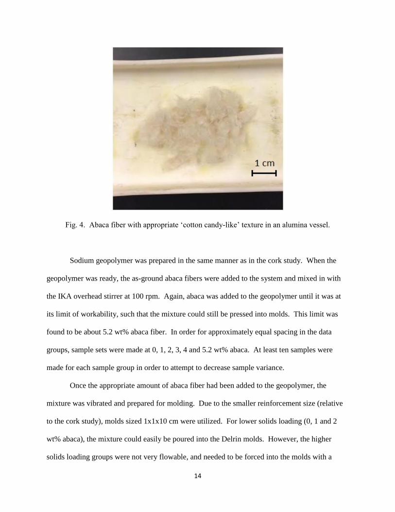
Fig. 4. Abaca fiber with appropriate ‘cotton candy-like’ texture in an alumina vessel.
Sodium geopolymer was prepared in the same manner as in the cork study. When the
geopolymer was ready, the as-ground abaca fibers were added to the system and mixed in with
the IKA overhead stirrer at 100 rpm. Again, abaca was added to the geopolymer until it was at
its limit of workability, such that the mixture could still be pressed into molds. This limit was
found to be about 5.2 wt% abaca fiber. In order for approximately equal spacing in the data
groups, sample sets were made at 0, 1, 2, 3, 4 and 5.2 wt% abaca. At least ten samples were
made for each sample group in order to attempt to decrease sample variance.
Once the appropriate amount of abaca fiber had been added to the geopolymer, the
mixture was vibrated and prepared for molding. Due to the smaller reinforcement size (relative
to the cork study), molds sized 1x1x10 cm were utilized. For lower solids loading (0, 1 and 2
wt% abaca), the mixture could easily be poured into the Delrin molds. However, the higher
solids loading groups were not very flowable, and needed to be forced into the molds with a

15
spatula. As before, molded samples were covered in plastic wrap, and placed into an oven at
50°C for 24 hours to set.
Upon removal from the curing oven, samples were demolded and immediately
mechanically tested. The same ASTM standard as noted in the cork study was used, with the
primary difference being the sample size. Lower supports were once again placed equidistant
from the points of load application. The outer span was set equal to 40 mm and the inner span
was 20 mm, following the same ratios of spans as seen in the cork study. The displacement rate
of the head continued to be adjusted throughout the experiment so as to keep the stress increase
in samples less than 1 MPa/min. Data from each sample group was recorded and plotted to
compare maximum flexural stress across each sample group. This data was also compared
against the potassium geopolymer abaca composite data.
2.3 Abaca Fiber Reinforced Potassium Geopolymer
2.3.1 Sample Preparation
The final system analyzed in this study was abaca fiber reinforced potassium
geopolymer. Potassium waterglass (K2O·2SiO2·11H2O) was created by mixing potassium
hydroxide and fumed silica with deionized water. The potassium waterglass was allowed to mix
for several hours on a magnetic stir place. As both potassium hydroxide and silica give off heat
when mixed with water, the entire mixture was massed once the waterglass had reached room
temperature. Any missing mass was assumed to be from evaporated water, and was replaced
with deionized water and mixed further. As with the sodium waterglass, the mixture was poured
into a plastic container and stored at 2°C once homogenously mixed. To prepare potassium
geopolymer, potassium waterglass was mixed with metakaolin in the ratio of 1.8574:1 mass

16
waterglass to metakaolin. The mixture was mixed and degassed as in the sodium geopolymer
studies.
Abaca fibers were produced from unbleached abaca sheets in the same manner as the
sodium geopolymer abaca study. Once more, abaca was added to the geopolymer until it was at
its limit of workability, such that the mixture could still be pressed into molds. Due to potassium
geopolymer’s lower viscosity (relative to sodium geopolymer), more abaca fiber could be mixed
into the geopolymer before the limit of workability was reached. This was hypothesized to lead
to an increase in flexural strength when compared to abaca fibers in sodium geopolymer. The
limit of workability was found to be 8 wt% abaca in potassium geopolymer. In order to generate
equal spacing between sample group data, samples were created at 0, 2, 4, 6 and 8 wt% abaca
fiber additions.
As in the abaca-sodium geopolymer system, once the appropriate amount of abaca fiber
had been added to the geopolymer, the mixture was vibrated and prepared for molding. Again,
molds sized 1x1x10 cm were utilized. For lower solids loading (0 and 2 wt% abaca), the mixture
could easily be poured into the Delrin molds. However, the higher solids loading groups were
not very flowable, and needed to be forced into the molds. This forcing was hypothesized to
contribute to larger macroscopic flaws as air bubbles could not be vibrated out of the thick, high
solids loaded samples. As before, molded samples were covered in plastic wrap, and placed into
an oven at 50°C for 24 hours to set. During removal from Delrin molds after setting, thin flakes
often chipped off the top of the sample, leading to surfaces with a rough appearance. These
chips, despite having a relatively small effect on sample height (usually 0.1-0.2 mm) were
nevertheless accounted for in the calculations of load carried in mechanical testing.

17
Mechanical testing was carried out in the same manner as in the abaca sodium
geopolymer system. In the following durability and heat treatment sections, all mechanical
testing was performed under the same conditions.
2.3.2 Durability Testing
In order to determine the durability of the samples, the highest solids loaded samples
were exposed to a number of harsh environments. Since no single standard existed for the acid,
base, water and freeze durability of biologically-reinforced geopolymers, experiments were
developed based on methodology presented in existing geopolymer durability papers [20].
Five different durability test were carried out. Four were ‘soaking’ tests: water, salt
water, sulfuric acid and sodium hydroxide durability. The fifth was a ‘cycle’ test: samples
subjected to a cycle of frozen and thawed water.
Each of the ‘soaking’ tests were carried out over a four-week period. In each instance,
twelve 8 wt% abaca samples were placed into the respective solutions for 14 days. After those
14 days, the samples were removed and allowed to dry at ambient room conditions for another
14 days. In the case of the ‘cycle’ test, twelve 8 wt% samples were placed into deionized water.
For the next 14 days, the water alternated spending 24 hours in a freezer at -4°C and 24 hours at
ambient room temperature. After those 14 days, the samples were removed and allowed to dry at
ambient room conditions for another 14 days.
The solutions for the durability tests were prepared in the following ways. “Water
durability” samples were merely added to deionized water. “Salt water durability” samples were
subjected to a mixture of deionized water and sodium chloride. The solution contained 7.5 wt%
sodium chloride. “Sodium hydroxide durability” samples were placed in a 1M NaOH solution

18
made by mixing NaOH pellets with deionized water. Finally, “sulfuric acid durability” samples
were subjected to 1M H2SO4 prepared by diluting concentrated sulfuric acid with deionized
water.
In each of the above experiments, samples were immediately mechanically tested at the
end of their respective 28-day period. These mechanical tests were carried out in an identical
fashion as the original abaca fiber reinforced potassium geopolymer samples. This new data was
compared to those original samples, and across all the sample groups in the durability study, then
plotted thusly.
2.3.3 Heat Treatment Testing
In order to determine the heat sensitivity of the highest solids loading samples, abaca
reinforced potassium geopolymer samples were subjected to a number of different heating
profiles. These heating profiles maxed out at 50°C, 100°C, 150°C, 200°C and 250°C. One
sample was subjected to 300°C in order to confirm that the composite would become structurally
compromised at that temperature.
In the case of each heating profile, the dozen samples were placed on an alumina vessel
without touching each other. The samples were then placed in a Fisher Scientific Isotemp
Programmable Muffle Furnace (Fisher Scientific, Pittsburgh, PA) and heated at 1°C per minute
until the maximum temperature was reached. At that point, the oven held the maximum
temperature for once hour. After the hold, the oven decreased the temperature by 1°C per minute
until room temperature was reached.

19
As with the durability testing, samples were removed after reaching room temperature
and mechanically tested in four-point flexure. The data gathered was plotted and compared to
original and durability study data.
To better understand when abaca fiber thermally degrades (and how effectively
potassium geopolymer thermally shielded its reinforcement), pure abaca fiber was treated to
identical heat profiles. The abaca fiber showed little visible change until the 200°C samples, and
was completely burnt by the 250°C heating profile. New abaca fiber was treated to a profile that
went to 240°C in order to more accurately predict the burning point of pure abaca fiber.
2.3.4 SEM Analysis
From each sample group, a fracture surface from one sample was analyzed in a scanning
electron microscope (SEM). Three main groups were studied: plain abaca samples (0, 2, 4, 6 and
8 wt%), heat treatment samples (50°C, 100°C, 150°C, 200°C, 250°C and 300°C) and durability
tested samples (water, salt water, sulfuric acid, sodium hydroxide and freeze cycle). When a
sample from each group was selected, the surface was removed from the bulk of the sample with
a circular saw approximately 1 cm from the fracture surface. These fracture surfaces were then
Au-sputter coated in a Denton Desktop Pro (Denton Vacuum, Moorestown, NJ).
Upon removal from the sputter coater, samples were loaded into a Neoscope 6000 Plus
SEM (Jeol, Peabody, MA). Samples were individually analyzed. The samples were subjected to
“high-vacuum” mode, and analyzed at 15 kV. For each of the sixteen samples analyzed, four
different magnifications were used: x24, x100, x500 and x1000. Images were then inspected for
abnormalities, fiber debonding, fiber pullout, and other composite phenomena.

20
2.3.5 XRD Analysis
X-ray Diffraction (XRD) was used in two separate instances in this study. The first was
to determine if potassium geopolymer had truly been prepared by comparing its XRD profile to
that of a known potassium geopolymer with fully reacted metakaolin. If the metakaolin in the
sample was not fully reacted, the amorphous humps noted in the XRD patterns would have been
offset.
To prepare potassium geopolymer for XRD analysis, a segment of approximately 1 cm3
of pure potassium geopolymer was taken and placed in a mortar and pestle. The geopolymer
was hand-ground to a very fine powder with the consistency of baking flour. The powder was
then placed on a slide and leveled per standard XRD practices.
The sample and its holder were placed into a Siemens Bruker 5000 X-ray diffractometer
(Siemens, Munich, Germany). Settings were as follows: scan from two theta values of 10° to
45°, step size 0.01°, time/step 0.5 seconds. Scans were then analyzed and compared to existing
patterns.
The second instance XRD was used was to identify an unknown crystal that appeared on
the potassium geopolymer-abaca composite during sulfuric acid durability testing. The crystals
were removed from the composite with a gloved hand, and any excess geopolymer stuck to the
crystals was carefully scraped off with a needle.
The crystals were ground in a mortar and pestle similarly to the potassium geopolymer,
and placed into the same XRD with identical step-size and time/step settings. The only
difference was the two theta range was a broader 0° to 60°. The pattern generated was compared
in a database to determine the chemical composition of the crystals.
21
CHAPTER 3
RESULTS AND DISCUSSION
3.1 Cork Particle Reinforced Sodium Geopolymer
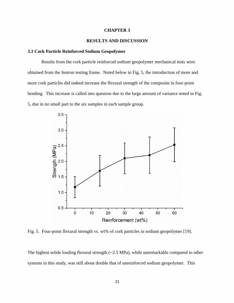
Results from the cork particle reinforced sodium geopolymer mechanical tests were
obtained from the Instron testing frame. Noted below in Fig. 5, the introduction of more and
more cork particles did indeed increase the flexural strength of the composite in four-point
bending. This increase is called into question due to the large amount of variance noted in Fig.
5, due in no small part to the six samples in each sample group.
Fig. 5. Four-point flexural strength vs. wt% of cork particles in sodium geopolymer [19].
The highest solids loading flexural strength (~2.5 MPa), while unremarkable compared to other
systems in this study, was still about double that of unreinforced sodium geopolymer. This

22
indicated good adhesion of the geopolymer to the reinforcement. A reason for the less-than-
desirable increase in flexural strength might have been the size of the samples: these 1”x1”x6”
samples were relatively large (compared to later studies), which statistically allowed for a greater
chance of critical flaws to exist within the sample. The slight increase in flexural strength was
also attributed to the fact that the nature of the cork particles allowed more than half of the
composite weight to be reinforcement. Since the cork was in particle form (seen below in Fig. 6)
on the millimeter scale, it was simple to pack a large quantity of reinforcement into the 1”x1”x6”
molds. This was not the case for later studies involving fibrous reinforcement, which tended to
self-interact, making the molding stages more difficult.
Fig. 6. Picture of cork particles used in sodium geopolymer composite (scale in picture is cm).
While the cork did not impress with its effect on the flexural strength of the composite, it
did yield some interesting strain to failure properties. In normal structural ceramics, strain to
failure is usually noted at about 0.1% strain. The cork reinforced composites with the highest
solids loading managed an average flexural strain to failure of 0.9%. Once again, this unique

23
property was attributed to the fact that so much cork could be added into these composites,
making it increasingly more cork-like and less brittle [19].
Fig. 7. Flexural stress vs. flexural strain plot for the first three samples of highest solids loading.
Fig. 8. Flexural stress vs. flexural strain plot for the final three samples of highest solids loading.
All in all, the cork particle reinforced sodium geopolymer did show an increase in
flexural strength with the addition of the plant matter. More interestingly, it also vastly increased
24
the strain to failure that is normally seen in brittle ceramic materials. Ultimately, it was
determined that a cork particle reinforced sodium geopolymer system, while interesting, was not
a structurally feasible material for more ceramic-like applications. Thus, the study moved on to
a new biological reinforcement of choice: abaca fibers.
3.2 Abaca Fiber Reinforced Sodium Geopolymer
After the cork study, an attempt was made to create a geopolymer composite with greater
strengths than previously seen. It was hypothesized that a reinforcement with extremely high
aspect ratio would provide the most load transfer per unit weight, allowing for composite
strengths to increase. Abaca, as an extremely strong fiber, seemed liked the perfect biological
reinforcement to choose.
As with the cork study, results from the mechanical testing of the abaca fiber reinforced
sodium geopolymer were collected via the Instron testing frame. Seen in Fig. 9, it was again
noted that an increase in biological reinforcement increased the flexural strength of the
composite in question.

25
Fig. 9. Four-point flexural strength for different wt% of abaca fibers in sodium geopolymer.
Variance in sample groups increased as wt% reinforcement increased, but unlike in the cork
study, a marked increase in strength was noted. Whereas unreinforced sodium geopolymer had
an average flexural strength of ~2.5 MPa, the maximum fiber reinforced composite exhibited
flexural strengths (~27 MPa) more than ten times greater than unreinforced composites.
These impressive increases in flexural strengths (when compared to the cork study) were
attributed to two main features: the strength of the fibers themselves, and the aspect ratio of the
fibers. Abaca fibers are one of the strongest natural fibers in the world, found to have tensile
strengths exceeding 500 MPa [21]. This obviously was an important distinction when comparing

26
composites containing relatively delicate cork particles. Furthermore, generally spherical cork
particles did not maximize the surface area of reinforcement in contact with geopolymer per unit
weight. Abaca fibers, however, were perfectly suited for such contact.
Fig. 10. SEM micrograph of abaca fibers used in geopolymer composites.
Fig. 11. SEM micrograph of a single abaca fiber.

27
Fig. 10 demonstrates the extreme aspect ratio inherent to the abaca fibers, while Fig. 11 shows
the scale of abaca fiber diameters to be around 10 µm. Fig. 10 also demonstrates the degree of
entanglement that the abaca fibers experience, discussed further in the abaca fiber reinforced
potassium geopolymer system.
SEM micrographs were also taken of the fracture surfaces of various samples to better
understand the modes of failure, and how well abaca fibers were dispersed within the
geopolymer matrix.
Fig. 12. Fracture surface of a 1 wt% abaca fiber reinforced sodium geopolymer composite.

28
Fig. 13. Fracture surface of a 3 wt% abaca fiber reinforced sodium geopolymer composite.
Fig. 14. Fracture surface of a 5 wt% abaca fiber reinforced sodium geopolymer composite.

29
As expected, images in the progression from 1 wt% abaca to 5 wt% abaca showed a proportional
increase in abaca fibers. Abaca fibers seemed to distribute themselves throughout the composite
in a relatively uniform fashion. This was important, as it was not known how the fibers would
interact when placed within the sodium geopolymer matrix and forced into the molds.
Fiber pullout is visible in all three reinforcement groups, indicating some degree of
composite toughening took place during the mechanical analysis. Microcracks can be seen
traversing around fibers, another indication of toughening throughout the testing process.
Finally, larger flaws can be seen (particularly in the 5 wt% image), likely a result of the difficult
nature associated with forcing the composite into molds due to fiber entanglement.
All in all, the abaca reinforced sodium geopolymer study was extremely promising.
Maximum fiber reinforcement yielded flexural strengths more than ten times greater than that of
unreinforced sodium geopolymer. Clearly, the addition of abaca fibers steadily increased the
strength of the composite. To reach even greater strengths, attempts were made to increase the
amount of abaca fiber that could be incorporated into geopolymer composites. Those attempts
constitute the remainder of this study.
3.3 Abaca Fiber Reinforced Potassium Geopolymer
3.3.1 Untreated Abaca Fiber Reinforced Potassium Geopolymer
It was hypothesized that potassium geopolymer, which is less viscous than sodium
geopolymer, would allow more abaca fibers to be added to a geopolymer matrix. By increasing
the weight percent of abaca fibers in the composite, it was further hypothesized that even greater
flexural strengths could be attained.

30
It was indeed found that potassium geopolymer could handle more abaca fibers before
reaching its limit of workability. That limit was found to be 8 wt% abaca fibers. In order to
increase the confidence in results from this study, at least twelve samples were made in each
sample group. Results from the flexural testing of the abaca reinforced potassium geopolymer
can be seen in Fig. 15.
Fig 15. Flexural strength vs. abaca weight percent in potassium geopolymer composites.
Clearly, the addition of abaca fiber had a large impact on the flexural strengths of
the composite samples. From unreinforced sample strengths around ~7 MPa, composite strength
continued to increase with added abaca fiber to above 50 MPa at the 8 wt% abaca level. The
increased number of samples in each group did help to reduce the variance in the less reinforced
31
samples, but large variance was still noted at the highest reinforcement. As with the other two
studies, variance increased as fiber reinforcement increased.
Despite this variance, an average flexural strength of 50 MPa was regarded as a success.
The flexural strength exceeded the average flexural strength of unreinforced geopolymers (2-7
MPa) by nearly an order of magnitude. With this new composite labeled a ‘success’, attempts
were made to characterize its properties, with emphasis on its durability and sensitivity to heat
treatments.
3.3.2 Durability of Abaca Fiber Reinforced Potassium Geopolymer
Two types of durability testing were conducted: tests where the samples were exposed to
a constant environment (H2SO4, NaOH, water and salt water), and a test where the samples were
exposed to a changing environment (freezing water cycle). As in the untreated abaca reinforced
potassium geopolymer study, each group contained at least twelve samples. Samples used in
durability testing were all fully reinforced with 8 wt% abaca fibers.
After 14 days of freezing and thawing, and another 14 days of drying, a picture was taken
of a sample to determine if any macroscale physical changes had occurred to the sample, as seen
below in Fig. 16.

32
Fig. 16. 10 cm-long freeze cycle sample after 28-day durability testing period.
Fig. 16 shows that no major macroscale damage or discoloration was caused by the freeze cycle.
Any imperfections noted on the edges existed previously as a result of the laborious molding
process.
After the freeze cycle (and subsequent drying), the samples were subjected to mechanical
testing as in previous studies. The result of that testing can be seen in Fig. 17.

33
Fig. 17. Flexural strength of abaca fiber reinforced potassium geopolymer after freeze cycle.
Despite the lack of macroscale flaws as a result of the freeze cycle, the overall strength of
the composite clearly suffered. As compared to the strength of untreated 8 wt% abaca fiber
reinforced potassium geopolymer samples (~50 MPa), the strength of the freeze cycle samples
was more than halved (~23 MPa). Microscale examination of the reasons attributed for this
decrease in strength is carried out in the later SEM section.
Pictures were similarly taken of the samples in the unchanging environments after 14
days of soaking and 14 days of drying, pictured below.

34
Fig. 18. 10 cm-long water durability sample after 28-day soaking period.
Fig. 19. 10 cm-long salt water durability sample after 28-day soaking period.

35
Fig. 20. 10 cm-long NaOH durability sample after 28-day soaking period.
Fig. 21. 10 cm-long H2SO4 durability sample after 28-day soaking period.

36
As with the freeze cycle samples, water, salt water and NaOH durability testing
failed to yield any obvious macroscopic defects as a result of their environments. H2SO4 testing,
however, caused samples to swell up, crack, and become extremely fragile. Because of this,
H2SO4 durability samples were not mechanically tested. Mechanical data for the other groups is
presented below.
Fig. 22. Flexural strength of durability-tested abaca-potassium geopolymer composite.
Water and salt water durability testing did very little to decrease the flexural
strength of the abaca fiber reinforced potassium geopolymer samples. This was viewed as

37
promising for structural or maritime applications of the composite, which might be frequently
exposed to such environments. However, NaOH durability testing nearly halved the flexural
strengths of the composite, similar to the results seen in the freeze cycle durability test.
As mentioned before, H2SO4 samples were not mechanically tested due to their negligible
strength. Upon closer inspection, it was noted that the crevices within the H2SO4 sample
contained a number of clear crystals, pictured below.
Fig 23. Crystals obtained from H2SO4 durability tested samples.
These crystals indicated that a chemical reaction had taken place during the durability testing,
effectively ruining the samples. To identify the composition of these crystals, they were ground
and subjected to XRD analysis. The results are shown below.

38
Fig. 24. XRD analysis of crystals determined to be KAl(SO4)2•12H2O.
XRD results best matched with alum, which has the chemical formula KAl(SO4)2•12H2O. The
~0.5 degree shift in Fig. 24 was likely due to tilt in the slide holder of the XRD. To confirm this
result, a simple stoichiometric exercise was carried out: the ratio of the molar mass of anhydrous
alum (258. 13 g/mol) and alum (462.24 g/mol) was determined to be 0.558. By weighing a large
crystal before heating (0.0732 g) and after an hour of being subjected to 110°C (0.0424 g), the
experimental ratio was found to be 0.579. This was within 4% of the theoretical value, thereby
confirming the crystal as alum.
3.3.3 Heat Treatment of Abaca Fiber Reinforced Potassium Geopolymer
To test the heat resistance of the abaca fiber reinforced potassium geopolymer composite,
samples were subjected to a variety of temperatures then mechanically tested as before. Once

39
more, each sample group contained a minimum of twelve samples, and pictures of samples were
taken before mechanical testing for qualitative analysis, seen below.
Fig. 25. 10 cm-long 100°C heat treated sample.
Fig. 26. 10 cm-long 150°C heat treated sample.

40
Fig. 27. 10 cm-long 200°C heat treated sample.
Fig. 28. 10 cm-long 250°C heat treated sample.
41
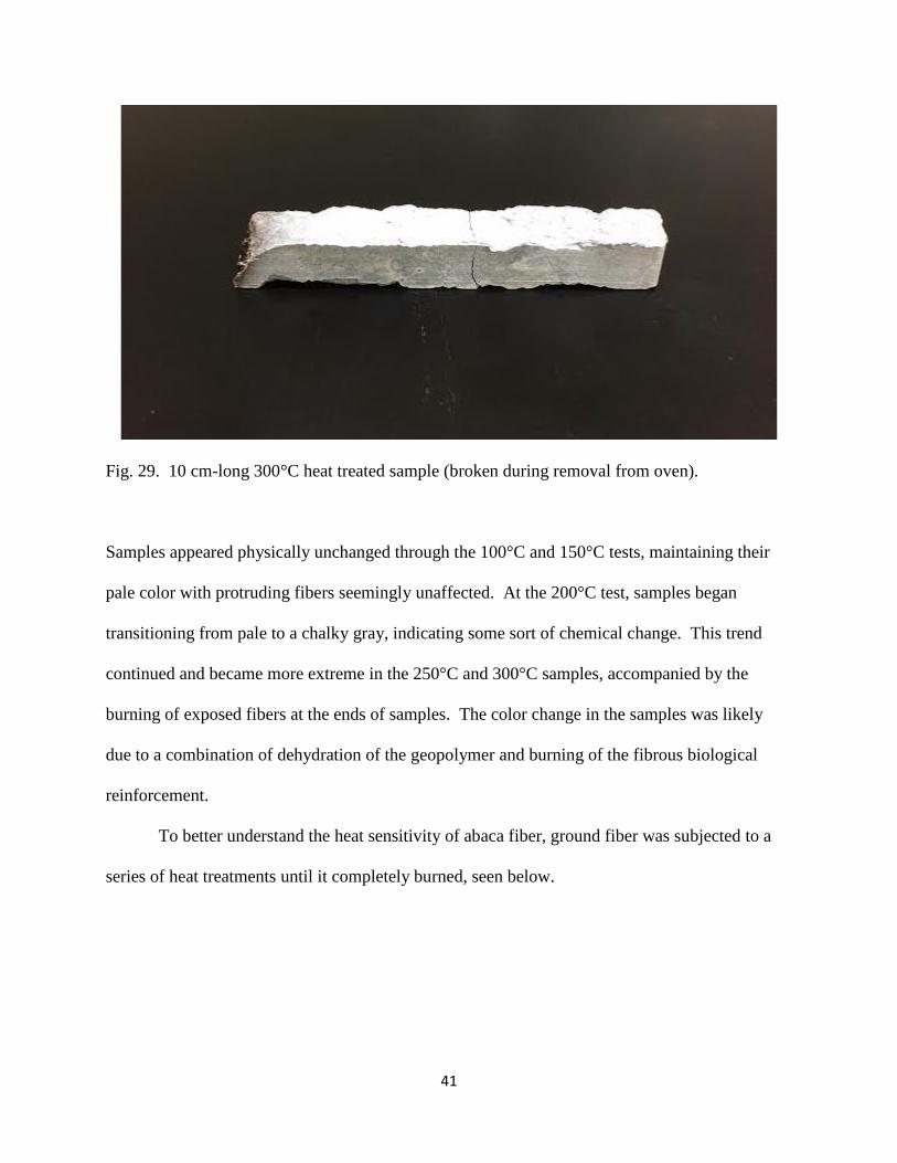
Fig. 29. 10 cm-long 300°C heat treated sample (broken during removal from oven).
Samples appeared physically unchanged through the 100°C and 150°C tests, maintaining their
pale color with protruding fibers seemingly unaffected. At the 200°C test, samples began
transitioning from pale to a chalky gray, indicating some sort of chemical change. This trend
continued and became more extreme in the 250°C and 300°C samples, accompanied by the
burning of exposed fibers at the ends of samples. The color change in the samples was likely
due to a combination of dehydration of the geopolymer and burning of the fibrous biological
reinforcement.
To better understand the heat sensitivity of abaca fiber, ground fiber was subjected to a
series of heat treatments until it completely burned, seen below.

42
Fig. 30. Abaca fiber before exposure to any temperature testing.
Fig 31. Abaca fiber after exposure to 225°C.

43
Fig 32. Abaca fiber after exposure to 250°C.
Very little discoloration was noted when the fiber was heated to 200°C. At 225°C, some
browning occurred on the fringes of the fiber. By 250°C, the fiber was nearly completed burnt,
and clearly past its burning point. In order to better determine the temperature at which abaca
fiber began to burn, a final test was conducted at 240°C, pictured below.
44
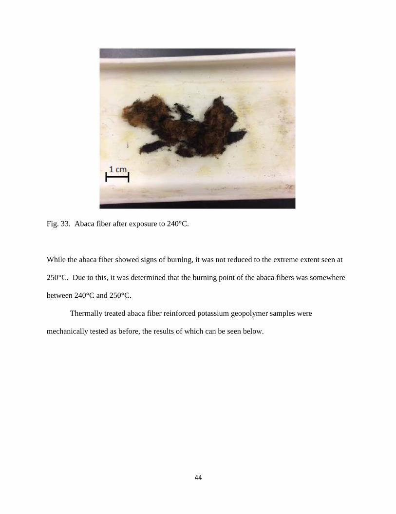
Fig. 33. Abaca fiber after exposure to 240°C.
While the abaca fiber showed signs of burning, it was not reduced to the extreme extent seen at
250°C. Due to this, it was determined that the burning point of the abaca fibers was somewhere
between 240°C and 250°C.
Thermally treated abaca fiber reinforced potassium geopolymer samples were
mechanically tested as before, the results of which can be seen below.

45
Fig 34. Flexural strength of heat treated abaca-potassium geopolymer composites.
As predicted, an increase in temperature that the abaca fiber reinforced potassium geopolymer
composites were exposed to decreased flexural strengths in the samples. This decrease was
likely initially caused by dehydration of the potassium geopolymer, and then later exacerbated by
the thermal degradation of the biological fiber at elevated temperatures.
As shown in Fig. 34, the composite lost almost all of its structural integrity by the 250°C
test, producing flexural strength values of just barely 1 MPa. However, at temperatures
experienced in nature, the abaca fiber reinforced potassium geopolymer composite still managed
impressive flexural strengths of over 35 MPa.

46
3.3.4 Weibull Statistical Analysis of Data
Weibull statistical analysis was employed to gain a better understanding of the
mechanical data obtained from each sample set. As described in the introduction, three graphs
were obtained for each sample group: a scatter plot of ln(ln(1/(1-F))) vs. ln(σf), a 95% confidence
interval probability plot, and a histogram of the samples in that group. Shown below are three
examples of those three graphs: one group from the untreated samples, one group from the
durability testing, and one group for the heat treatment testing. The graphs for all sample groups
can be found in the Appendix.
Fig. 35. Plot of ln(ln(1/(1-F))) vs. ln(σf) for 8 wt% abaca-reinforced potassium geopolymer.

47
Fig. 36. Probability plot of 8 wt% abaca-reinforced potassium geopolymer.
Fig. 37. Histogram of 8 wt% abaca-reinforced potassium geopolymer.

48
Fig. 38. Plot of ln(ln(1/(1-F))) vs. ln(σf) for composite heated to 150°C.
Fig. 39. Probability plot of abaca-reinforced potassium geopolymer heated to 150°C.

49
Fig. 40. Histogram of abaca-reinforced potassium geopolymer heated to 150°C.
Fig. 41. Plot of ln(ln(1/(1-F))) vs. ln(σf) for composite treated with NaOH.

50
Fig. 42. Probability plot of abaca-reinforced potassium geopolymer treated with NaOH.
Fig. 43. Histogram of abaca-reinforced potassium geopolymer treated with NaOH.

51
The data from these graphs were used to make a comprehensive table comparing
Weibull modulus, scale parameter, Weibull average, standard deviation and the 95% confidence
interval across all sample groups studied, as seen below.

52
Table 3. Weibull statistics of four-point flexure of abaca fiber reinforced potassium geopolymer.
Sample Group
Weibull Modulus
Scale Parameter
(MPa)
Weibull Average (MPa)
Standard Deviation
(MPa)
95% Confidence
Interval (MPa)
0 wt% Abaca
4.917 8.65 7.94 1.85 7.07, 8.85
2 wt% Abaca
5.323 13.11 12.09 2.61 10.90, 13.42
4 wt% Abaca
4.668 30.47 27.87 6.79 25.11, 31.06
6 wt% Abaca
5.101 37.44 34.42 7.74 30.05, 38.83
8 wt% Abaca
5.816 56.28 52.12 10.39 46.93, 57.80
50°C 3.824 41.05 37.11 10.82 31.42, 44.41
100°C 3.334 34.98 31.39 10.37 25.78, 38.21
150°C 3.435 19.86 17.85 5.74 14.59, 21.84
200°C 3.219 7.13 6.38 2.18 5.16, 7.89
250°C 4.031 1.36 1.23 0.34 1.04, 1.45
NaOH 2.433 30.22 26.80 11.74 20.65, 34.79
Water 3.537 53.55 48.21 15.11 40.00, 58.10
Salt water
3.222 52.84 47.34 16.14 39.03, 57.43
Freeze-Thaw Cycle
6.250 25.65 23.85 4.45 20.95, 27.16

53
3.3.5 SEM Analysis of Fracture Surfaces
SEM micrographs were taken at four magnifications for the fracture surfaces of one
sample from each sample group. A few images of note are presented here, but each SEM
micrograph of each fracture surface can be found in the Appendix.
Fig. 44. SEM micrograph of pore in potassium geopolymer at magnification x500.
In Fig. 44, an image of a large defect in an unreinforced potassium geopolymer sample is
noted. Imperfections such as this one contributed to lower than theoretical strength values, and
were hypothesized to occur more in higher wt% abaca samples as they became less workable and
more difficult to mold.

54
Fig 45. SEM micrograph of a 4 wt% reinforced composite at magnification x100.
Fig. 45 demonstrates that, as in the abaca fiber reinforced sodium geopolymer study, the
abaca fibers distributed themselves fairly evenly throughout the composite. This detail was
important in mechanical testing, as significant results rely on the material being as homogenous
and as uniform as possible.

55
Fig. 46. SEM micrograph of 8 wt% reinforced composite heated to 300°C, magnification x1000.
In Fig. 46, it is clear that elevated temperatures significantly reduced the diameter of
fibers in the composite. Fibers can be seen to have shrunk in from the walls of the matrix, which
provides an explanation as to why the composite had an essentially negligible flexural strength
after being exposed to such temperatures.
56
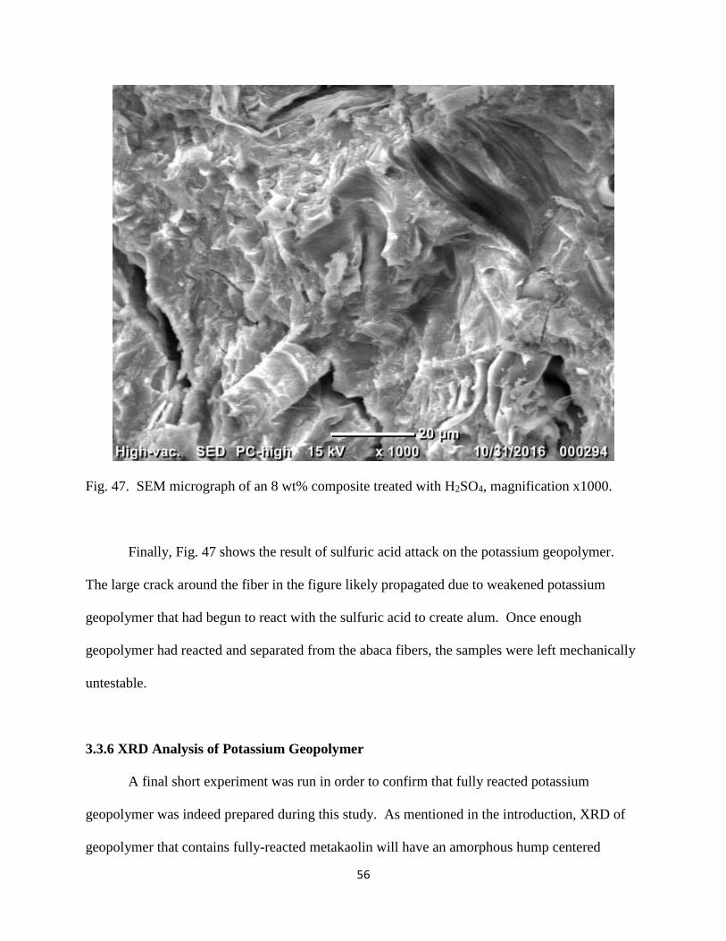
Fig. 47. SEM micrograph of an 8 wt% composite treated with H2SO4, magnification x1000.
Finally, Fig. 47 shows the result of sulfuric acid attack on the potassium geopolymer.
The large crack around the fiber in the figure likely propagated due to weakened potassium
geopolymer that had begun to react with the sulfuric acid to create alum. Once enough
geopolymer had reacted and separated from the abaca fibers, the samples were left mechanically
untestable.
3.3.6 XRD Analysis of Potassium Geopolymer
A final short experiment was run in order to confirm that fully reacted potassium
geopolymer was indeed prepared during this study. As mentioned in the introduction, XRD of
geopolymer that contains fully-reacted metakaolin will have an amorphous hump centered

57
around a two theta value of 28.5 degrees. A hump that was shifted significantly from that value
would indicate that the geopolymer was prepared improperly, and contained partially unreacted
metakaolin. XRD analysis of ground potassium geopolymer yielded the following results:
Fig. 48. XRD spectra of pure potassium geopolymer.
As Fig. 48 shows, the amorphous hump is indeed centered about two theta = 28.5 degrees. This
indicates that the abaca fiber reinforced potassium geopolymer composites in this study were
made with ideal matrix geopolymer.

58
CHAPTER 4
CONCLUSION
“Biologically reinforced geopolymers” is a broad topic which could be researched at
great length. This study managed to explore a few such systems, and characterized their
properties and viability as structural ceramic composites.
Cork reinforced sodium geopolymer improved from ~1.25 MPa to ~2.5 MPa (when taken
from unreinforced to 60 wt% cork). This composite system, while not a structurally viable
material, did yield interesting strain-to-failure results. The highest reinforced group managed
average strain-to-failure of 0.9% in flexure, about 9 times greater than expected for a normal
brittle ceramic.
Abaca fiber reinforced sodium geopolymer proved to be more viable as a structural
ceramic composite. Sodium-based geopolymer composites at the limit of workability (5.2 wt%
abaca fiber) demonstrated flexural strengths above 25 MPa, about 4-5 times stronger than
flexural strengths associated with OPCs. An attempt to infuse even more abaca fibers into
geopolymer led to the use of potassium geopolymer, known to be much less viscous than its
sodium counterpart.
Abaca fiber reinforced potassium geopolymer yielded an average flexural strength of 52
MPa at 8 wt% abaca fiber, a vast improvement over OPCs. These same composites
demonstrated good water and saltwater durability, decent NaOH and freeze cycle durability, and
poor H2SO4 durability. Additionally, these composites exhibited good strength retention at
temperatures experienced in nature. However, the composite did show a steady decrease in
flexural strength at more extreme temperatures due to dehydration and thermal degradation,
eventually losing all structural integrity by 300°C.

59
Several possible avenues for future work exist within this study. To increase the
strengths of the abaca fiber reinforced potassium geopolymer composites, more abaca fiber could
be added in a variety of ways. One such method might be by employing injection molding
methods, which would be doubly effective: injection molding would shear the shear-thinning
potassium geopolymer, lowering its viscosity and allowing more abaca fibers to be incorporated
into the composite. Injection molding would also help eliminate macroscale defects associated
with the current layup of the composite into Delrin molds.
Another area requiring more research is the testing of larger samples. If this composite is
to reach commercial applications in structures, it has to be proven to be effective at larger sizes
when critical flaws are more statistically likely. Confirmation of elevated strengths at larger
sample sizes would improve confidence in this composite as a viable structural ceramic.
Biologically reinforced geopolymers certainly have potential as a green structural
alternative to OPCs. Abaca fiber reinforced potassium geopolymer, while still in its infancy as a
characterized material, is at the forefront of biologically reinforced geopolymers with potential
as a commercial structural material.

60
CHAPTER 5
REFERENCES
1. J. Davidovits, “Mineral Polymers and Methods of Making Them”; U.S. Patent 4,349,386,
September 14, (1982).
2. J. Davidovits, “Geopolymers - Inorganic Polymeric New Materials,” J. Therm. Anal. 37 1633-
1656 (1991).
3. J. Davidovits, “Geopolymer Chemistry and Properties”; pp.25-48 in Geopolymer’88 First
European Conference on Soft Mineralogy, Vol.1 Edited by J. Davidovits and J. Orlinski.
Geopolymer Institute and Technical University, Compiegne, France, (1988).
4. J. Davidovits, Geopolymer Chemistry and Applications, 4th Edition (2015), published by the
Geopolymer Institute, St. Quentin, France.
5. V. F. F. Barbosa, and K. J. D. MacKenzie, “Synthesis and Thermal Behaviour of Potassium
Sialate Geopolymers,” Materials Letters, 57, 1477–82 (2003).
6. W. M. Kriven, J. L. Bell and M. Gordon, “Microstructure and Microchemistry of Fully-
Reacted Geopolymers and Geopolymer Matrix Composites,” Ceramic Transactions vol. 153,
227-250 (2003).
7. P. Duxson, J. L. Provis, G. C. Lukey, S. W. Mallicoat, W. M. Kriven and J. S. J. van Deventer,
“Understanding the Relationship between Geopolymer Composition, Microstructure and
Mechanical Properties,” Colloids and Surfaces A – Physicochemical and Engineering Aspects
269 [1-3] 47-58 (2005).
8. W. M. Kriven, J. L. Bell, S. W. Mallicoat and M. Gordon, “Intrinsic Microstructure and
Properties of Metakaolin-Based Geopolymers,” Proc. Int. Workshop on Geopolymer Binders –
Interdependence of Composition, Structure and Properties, Weimar, Germany. Published by the
Geopolymer Institute, St. Quentin, France 71-86 (2007).
9. J. L. Bell, P. Sarin, J. L. Provis, R. P. Haggerty, P. E. Driemeyer, P. J. Chupas, J. S. J. van
Deventer and W. M. Kriven, “Atomic Structure of a Cesium Aluminosilicate Geopolymer: A
Pair Distribution Function Study,” Chemistry of Materials, 20 [14] 4768-4776 (2008).
10. J. L. Bell, P. Sarin, P. E. Driemeyer, R. P. Haggerty, P. J. Chupas and W. M. Kriven, “X-ray
Pair Distribution Function Analysis of Potassium Based Geopolymer,” J. Materials Chemistry,
18 [48], 5974 - 5981 (2008).
11. W. M. Kriven, “Inorganic Polysialates or “Geopolymers,” American Ceramic Society
Bulletin, 89 [4] 31-34 (2010).

61
12. Geopolymer-based Composites,” W. M. Kriven, in Vol. 5, Ceramics and Carbon Matrix
Composites, edited by Marina Ruggles-Wrenn. Part of an 8 volume set of books
entitled Comprehensive Composite Materials II, Peter Beaumont and Carl Zweben, Co-editors-
in-chief. Published by Elsevier, Oxford, UK, in press (2017).
13. V. F. F. Barbosa, K. J. D. MacKenzie, “Thermal Behavior of Inorganic Geopolymers and
Composites Derived from Sodium Polysialate,” Mater. Res. Bull, 38, 319-331 (2003).
14. D. S. Roper, G. P. Kutyla and W. M. Kriven, “Properties of Granite Powder Reinforced
Geopolymer Composites,” Cer. Eng. and Sci. Proc., 36 [8] 3-10 (2015).
15. ASTM C1161-13, Standard Test Method for Flexural Strength of Advanced Ceramics at
Ambient Temperature, ASTM International, West Conshohocken, PA, 2013, DOI:
10.1520/C1161
16. Durability of Fly Ash Based Geopolymer Concrete Against Sulphuric Acid Attack:
International Conference On Durability of Building Materials and Components, Lyon, France
17-20 April (2005).
17. M. Hüsnü Dirikolu, Alaattin Aktas and Burak Birgören, “Statistical Analysis of Fracture
Strength of Composite Materials Using Weibull Distribution,” Turkish J. Eng. Env. Sci ., 26 45-
48 (2002).
18. Ross P. Williams, Robert D. Hart, and Arie van Riessen, “Quantification of the Extent of
Reaction of Metakaolin-Based Geopolymers Using X-Ray Diffraction, Scanning Electron
Microscopy, and Energy-Dispersive Spectroscopy,” J. Am. Ceram. Soc., 94 [8] 2663–2670
(2011).
19. D. S. Roper, G. P. Kutyla and W. M. Kriven, “Properties of Cork Particle Reinforced Sodium
Geopolymer Composites”, Cer. Eng. and Sci. Proc., 37 [7] 79-82 (2016).
20. Faiz Uddin Ahmed Shaikh, “Mechanical and Durability Properties of Fly Ash Geopolymer
Concrete Containing Recycled Coarse Aggregates”, International Journal of Sustainable Built
Environment, 5 [2] 277–287 (2016).
21. Alfred Noufie Mekel, Rudy Soenoko, Wahyono Suprapto and Anindito Purnowidodo,
“Tensile Strength of Abaca Strands from Sangihe Talaud Islands”, ARPN Journal of Engineering
and Applied Sciences, 11 [15] 9487-9490 (2016).

62
CHAPTER 6
APPENDIX: WEIBULL GRAPHS AND SEM MICROGRAPHS
Fig. 49. Scatterplot of ln(ln(1/(1-F))) vs ln(σ) for 0 wt% abaca-potassium geopolymer.
Fig. 50. 95% confidence interval probability plot for 0 wt% abaca-potassium geopolymer.

63
Fig. 51. Weibull fit to histogram for 0 wt% abaca-potassium geopolymer.
Fig. 52. Scatterplot of ln(ln(1/(1-F))) vs ln(σ) for 2 wt% abaca-potassium geopolymer.
64
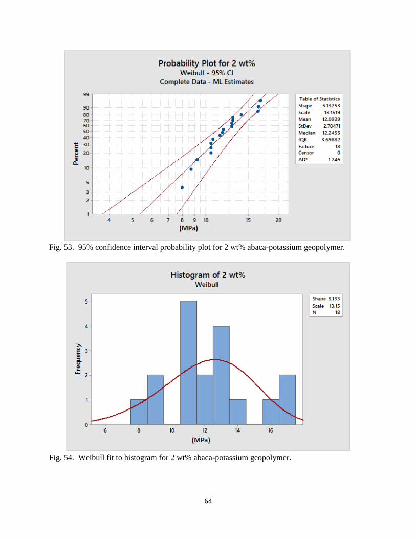
Fig. 53. 95% confidence interval probability plot for 2 wt% abaca-potassium geopolymer.
Fig. 54. Weibull fit to histogram for 2 wt% abaca-potassium geopolymer.

65
Fig. 55. Scatterplot of ln(ln(1/(1-F))) vs ln(σ) for 4 wt% abaca-potassium geopolymer.
Fig. 56. 95% confidence interval probability plot for 4 wt% abaca-potassium geopolymer.

66
Fig. 57. Weibull fit to histogram for 4 wt% abaca-potassium geopolymer.
Fig. 58. Scatterplot of ln(ln(1/(1-F))) vs ln(σ) for 6 wt% abaca-potassium geopolymer.
67
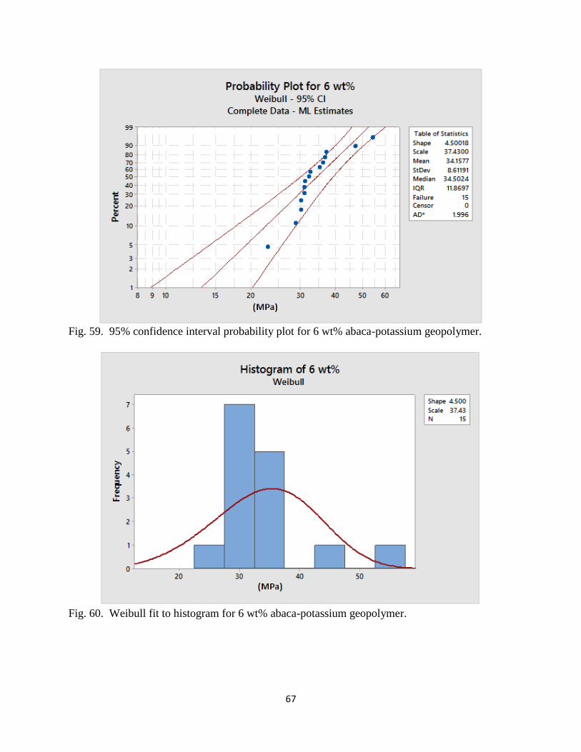
Fig. 59. 95% confidence interval probability plot for 6 wt% abaca-potassium geopolymer.
Fig. 60. Weibull fit to histogram for 6 wt% abaca-potassium geopolymer.

68
Fig. 61. Scatterplot of ln(ln(1/(1-F))) vs ln(σ) for 8 wt% abaca-potassium geopolymer.
Fig. 62. 95% confidence interval probability plot for 8 wt% abaca-potassium geopolymer.

69
Fig. 63. Weibull fit to histogram for 8 wt% abaca-potassium geopolymer.
Fig. 64. Scatterplot of ln(ln(1/(1-F))) vs ln(σ) for 50°C heat-treated samples.

70
Fig. 65. 95% confidence interval probability plot for 50°C heat-treated samples.
Fig. 66. Weibull fit to histogram for 50°C heat-treated samples.

71
Fig. 67. Scatterplot of ln(ln(1/(1-F))) vs ln(σ) for 100°C heat-treated samples.
Fig. 68. 95% confidence interval probability plot for 100°C heat-treated samples.

72
Fig. 69. Weibull fit to histogram for 100°C heat-treated samples.
Fig. 70. Scatterplot of ln(ln(1/(1-F))) vs ln(σ) for 150°C heat-treated samples.

73
Fig. 71. 95% confidence interval probability plot for 150°C heat-treated samples.
Fig. 72. Weibull fit to histogram for 150°C heat-treated samples.
74
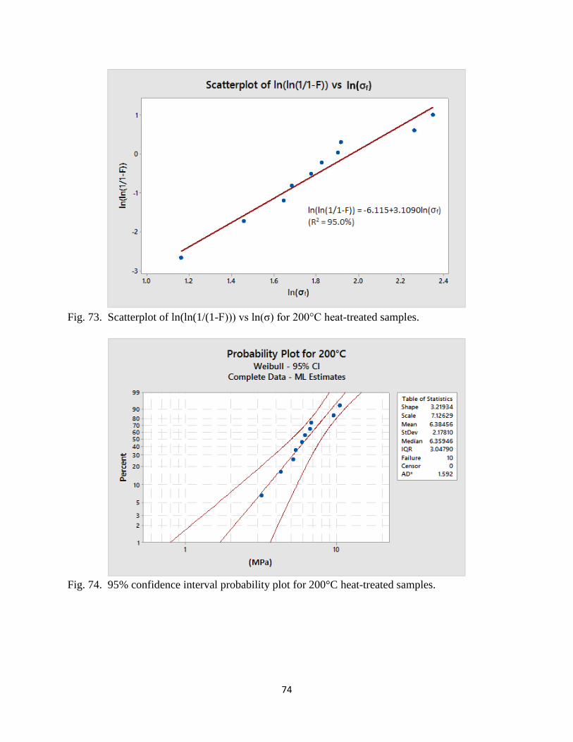
Fig. 73. Scatterplot of ln(ln(1/(1-F))) vs ln(σ) for 200°C heat-treated samples.
Fig. 74. 95% confidence interval probability plot for 200°C heat-treated samples.

75
Fig. 75. Weibull fit to histogram for 200°C heat-treated samples.
Fig. 76. Scatterplot of ln(ln(1/(1-F))) vs ln(σ) for 250°C heat-treated samples.

76
Fig. 77. 95% confidence interval probability plot for 250°C heat-treated samples.
Fig. 78. Weibull fit to histogram for 250°C heat-treated samples.

77
Fig. 79. Scatterplot of ln(ln(1/(1-F))) vs ln(σ) for NaOH durability samples.
Fig. 80. 95% confidence interval probability plot for NaOH durability samples.

78
Fig. 81. Weibull fit to histogram for NaOH durability samples.
Fig. 82. Scatterplot of ln(ln(1/(1-F))) vs ln(σ) for water durability samples.

79
Fig. 83. 95% confidence interval probability plot for water durability samples.
Fig. 84. Weibull fit to histogram for water durability samples.

80
Fig. 85. Scatterplot of ln(ln(1/(1-F))) vs ln(σ) for salt water durability samples.
Fig. 86. 95% confidence interval probability plot for salt water durability samples.
81
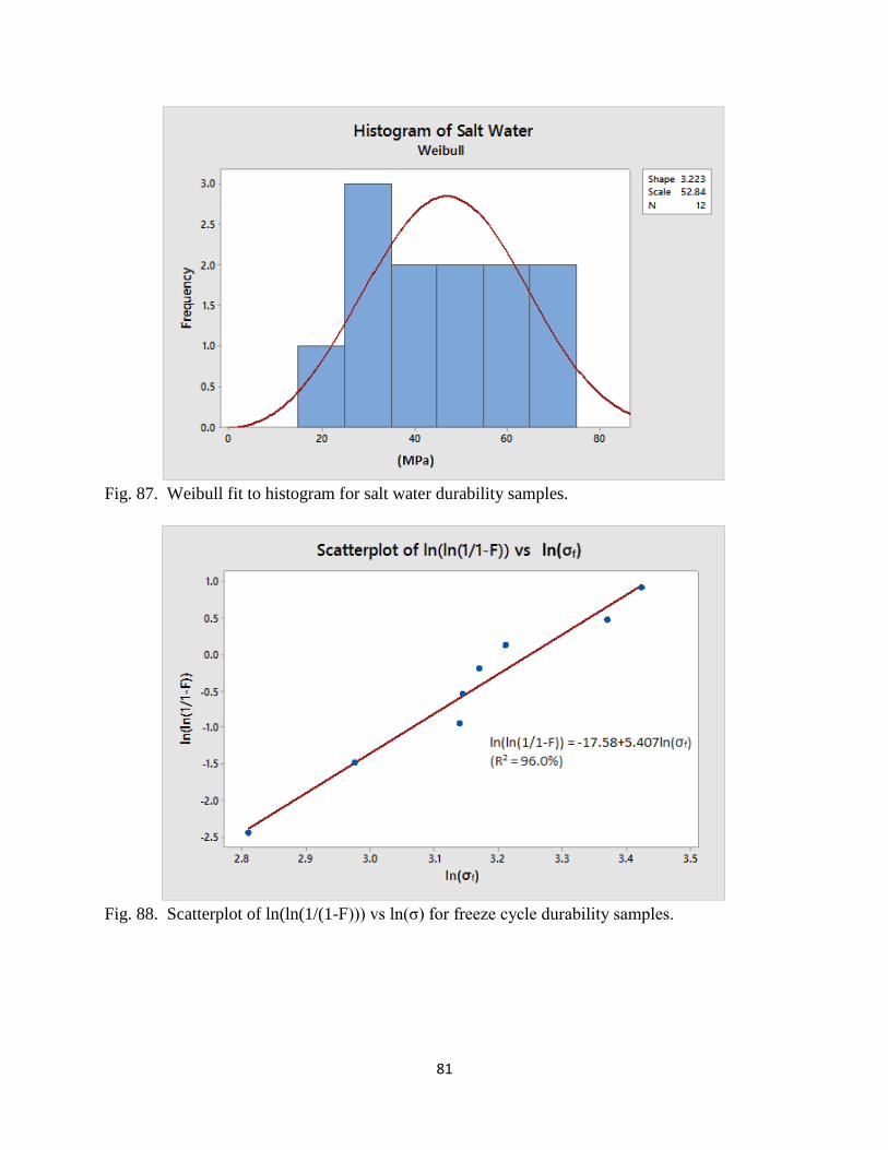
Fig. 87. Weibull fit to histogram for salt water durability samples.
Fig. 88. Scatterplot of ln(ln(1/(1-F))) vs ln(σ) for freeze cycle durability samples.

82
Fig. 89. 95% confidence interval probability plot for freeze cycle durability samples.
Fig. 90. Weibull fit to histogram for freeze cycle durability samples.
83
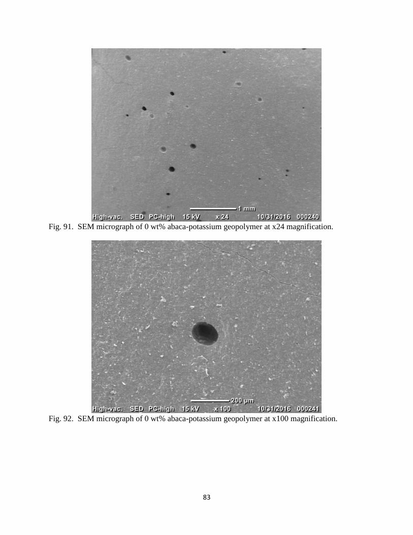
Fig. 91. SEM micrograph of 0 wt% abaca-potassium geopolymer at x24 magnification.
Fig. 92. SEM micrograph of 0 wt% abaca-potassium geopolymer at x100 magnification.

84
Fig. 93. SEM micrograph of 0 wt% abaca-potassium geopolymer at x500 magnification.
Fig. 94. SEM micrograph of 0 wt% abaca-potassium geopolymer at x1000 magnification.
85
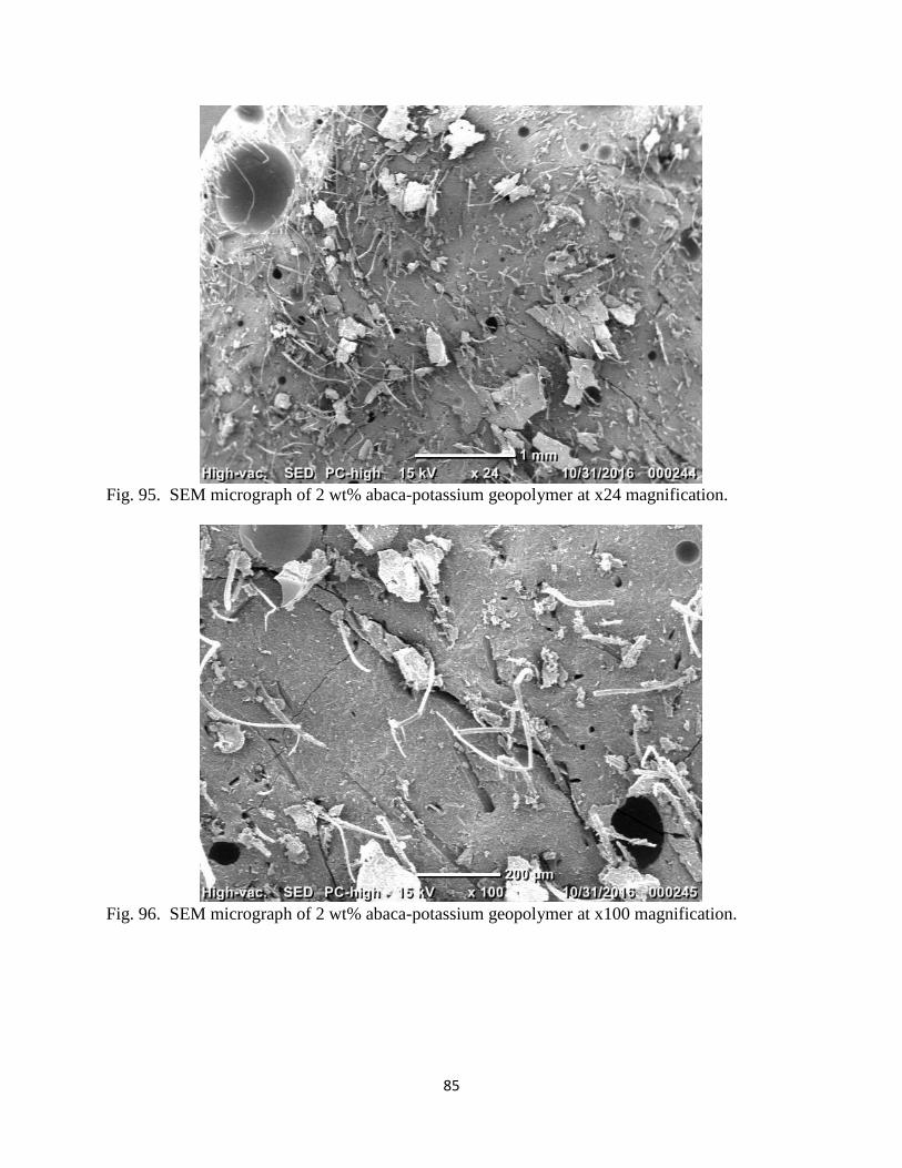
Fig. 95. SEM micrograph of 2 wt% abaca-potassium geopolymer at x24 magnification.
Fig. 96. SEM micrograph of 2 wt% abaca-potassium geopolymer at x100 magnification.

86
Fig. 97. SEM micrograph of 2 wt% abaca-potassium geopolymer at x500 magnification.
Fig. 98. SEM micrograph of 2 wt% abaca-potassium geopolymer at x1000 magnification.

87
Fig. 99. SEM micrograph of 4 wt% abaca-potassium geopolymer at x27 magnification.
Fig. 100. SEM micrograph of 4 wt% abaca-potassium geopolymer at x100 magnification.

88
Fig. 101. SEM micrograph of 4 wt% abaca-potassium geopolymer at x500 magnification.
Fig. 102. SEM micrograph of 4 wt% abaca-potassium geopolymer at x1000 magnification.
89
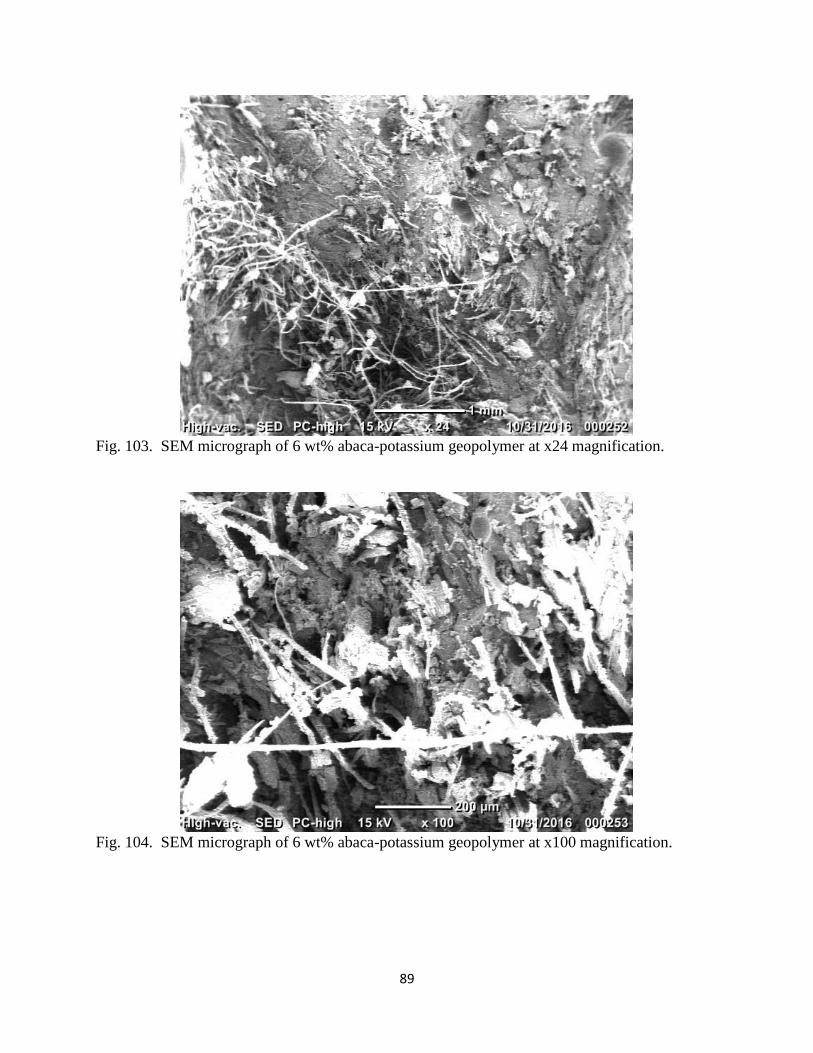
Fig. 103. SEM micrograph of 6 wt% abaca-potassium geopolymer at x24 magnification.
Fig. 104. SEM micrograph of 6 wt% abaca-potassium geopolymer at x100 magnification.

90
Fig. 105. SEM micrograph of 6 wt% abaca-potassium geopolymer at x500 magnification.
Fig. 106. SEM micrograph of 6 wt% abaca-potassium geopolymer at x1000 magnification.

91
Fig. 107. SEM micrograph of 8 wt% abaca-potassium geopolymer at x24 magnification.
Fig. 108. SEM micrograph of 8 wt% abaca-potassium geopolymer at x100 magnification.

92
Fig. 109. SEM micrograph of 8 wt% abaca-potassium geopolymer at x500 magnification.
Fig. 110. SEM micrograph of 8 wt% abaca-potassium geopolymer at x1000 magnification.

93
Fig. 111. SEM micrograph of 50°C heat treated sample at x24 magnification.
Fig. 112. SEM micrograph of 50°C heat treated sample at x100 magnification.
94
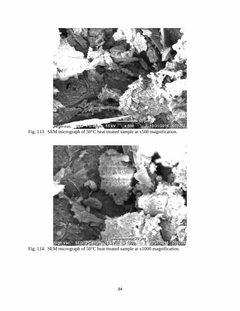
Fig. 113. SEM micrograph of 50°C heat treated sample at x500 magnification.
Fig. 114. SEM micrograph of 50°C heat treated sample at x1000 magnification.

95
Fig. 115. SEM micrograph of 100°C heat treated sample at x24 magnification.
Fig. 116. SEM micrograph of 100°C heat treated sample at x100 magnification.

96
Fig. 117. SEM micrograph of 100°C heat treated sample at x500 magnification.
Fig. 118. SEM micrograph of 100°C heat treated sample at x1000 magnification.

97
Fig. 119. SEM micrograph of 150°C heat treated sample at x24 magnification.
Fig. 120. SEM micrograph of 150°C heat treated sample at x100 magnification.
98
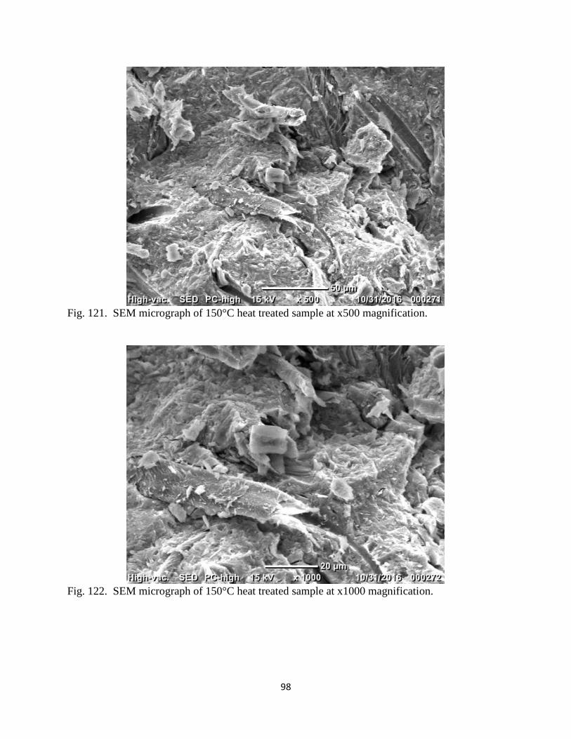
Fig. 121. SEM micrograph of 150°C heat treated sample at x500 magnification.
Fig. 122. SEM micrograph of 150°C heat treated sample at x1000 magnification.

99
Fig. 123. SEM micrograph of 200°C heat treated sample at x24 magnification.
Fig. 124. SEM micrograph of 200°C heat treated sample at x100 magnification.

100
Fig. 125. SEM micrograph of 200°C heat treated sample at x500 magnification.
Fig. 126. SEM micrograph of 200°C heat treated sample at x1000 magnification.

101
Fig. 127. SEM micrograph of 250°C heat treated sample at x24 magnification.
Fig. 128. SEM micrograph of 250°C heat treated sample at x100 magnification.

102
Fig. 129. SEM micrograph of 250°C heat treated sample at x500 magnification.
Fig. 130. SEM micrograph of 250°C heat treated sample at x1000 magnification.

103
Fig. 131. SEM micrograph of 300°C heat treated sample at x24 magnification.
Fig. 132. SEM micrograph of 300°C heat treated sample at x100 magnification.

104
Fig. 133. SEM micrograph of 300°C heat treated sample at x500 magnification.
Fig. 134. SEM micrograph of 300°C heat treated sample at x1000 magnification.
105
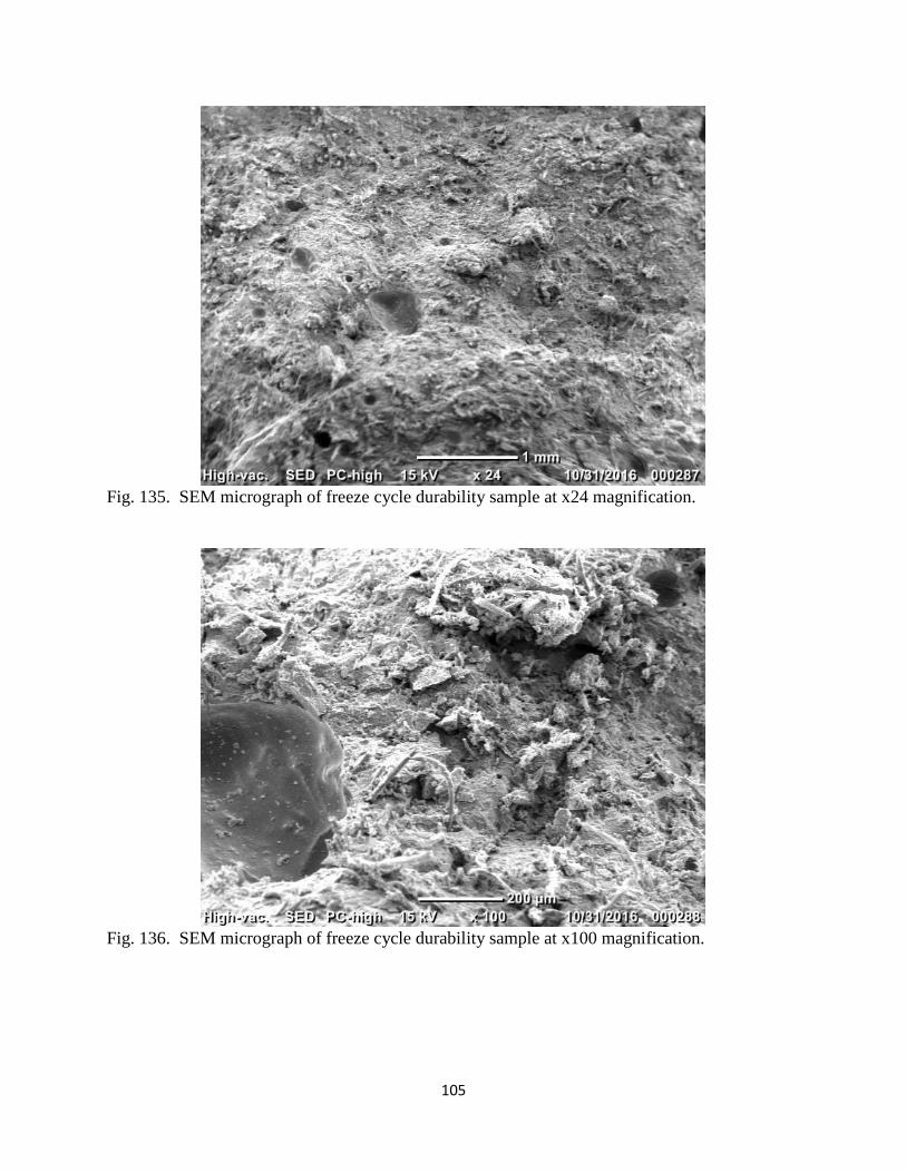
Fig. 135. SEM micrograph of freeze cycle durability sample at x24 magnification.
Fig. 136. SEM micrograph of freeze cycle durability sample at x100 magnification.
106
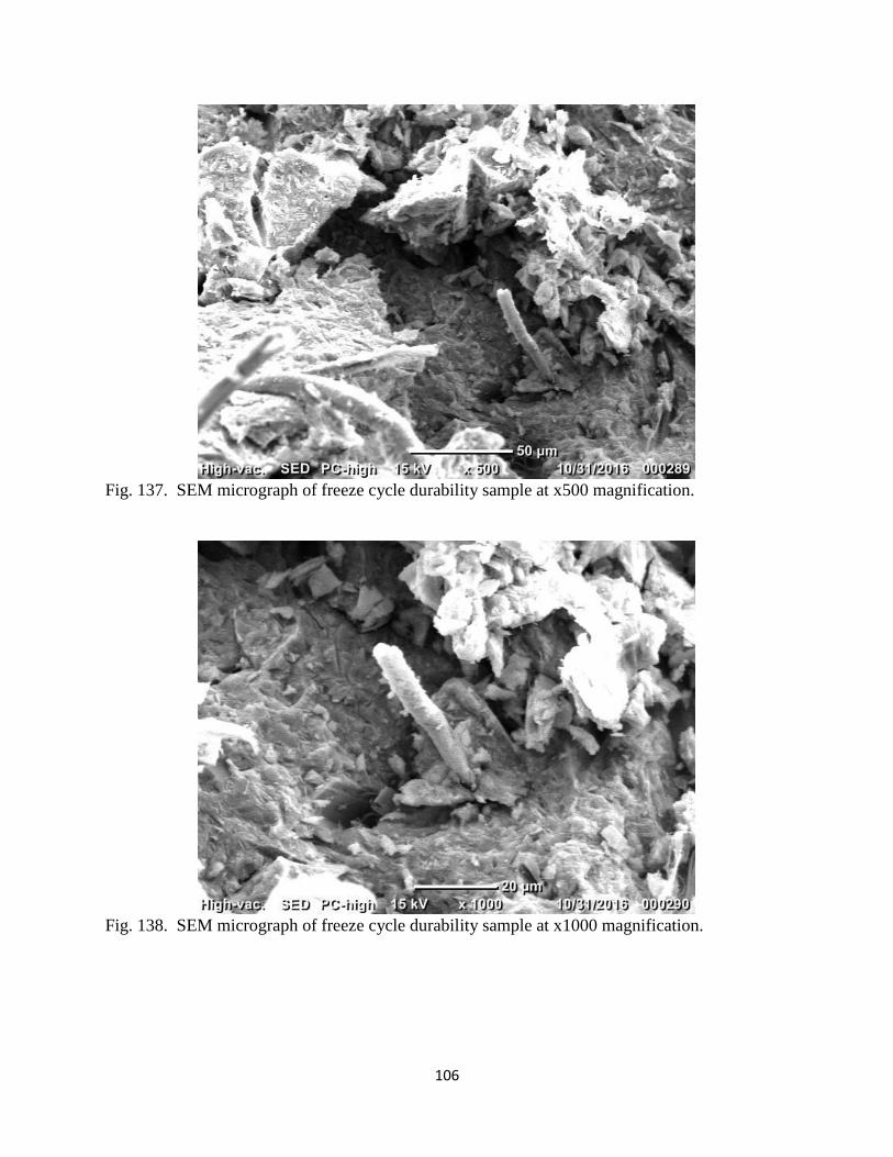
Fig. 137. SEM micrograph of freeze cycle durability sample at x500 magnification.
Fig. 138. SEM micrograph of freeze cycle durability sample at x1000 magnification.

107
Fig. 139. SEM micrograph of H2SO4 durability sample at x24 magnification.
Fig. 140. SEM micrograph of H2SO4 durability sample at x100 magnification.

108
Fig. 141. SEM micrograph of H2SO4 durability sample at x500 magnification.
Fig. 142. SEM micrograph of H2SO4 durability sample at x1000 magnification.
109
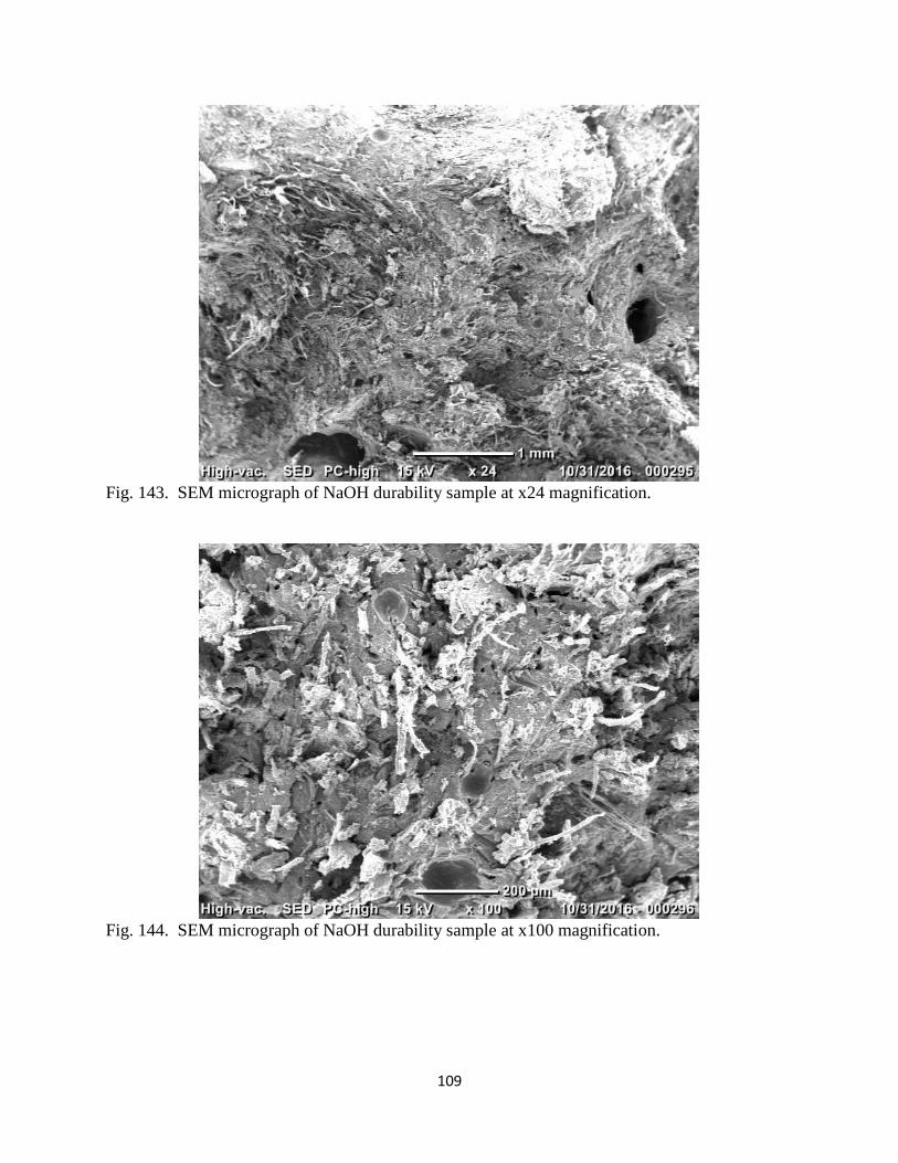
Fig. 143. SEM micrograph of NaOH durability sample at x24 magnification.
Fig. 144. SEM micrograph of NaOH durability sample at x100 magnification.
110
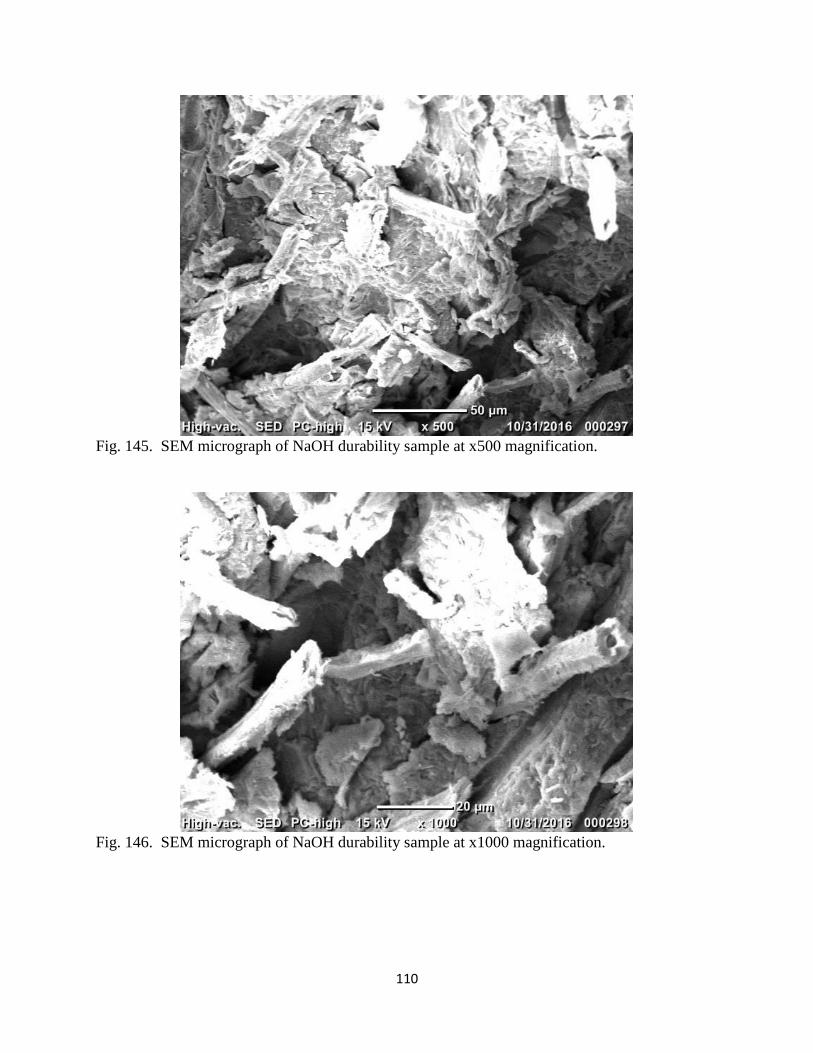
Fig. 145. SEM micrograph of NaOH durability sample at x500 magnification.
Fig. 146. SEM micrograph of NaOH durability sample at x1000 magnification.
111
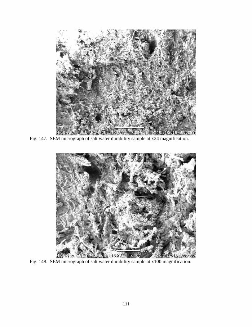
Fig. 147. SEM micrograph of salt water durability sample at x24 magnification.
Fig. 148. SEM micrograph of salt water durability sample at x100 magnification.
112
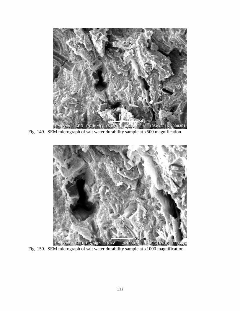
Fig. 149. SEM micrograph of salt water durability sample at x500 magnification.
Fig. 150. SEM micrograph of salt water durability sample at x1000 magnification.

113
Fig. 151. SEM micrograph of water durability sample at x24 magnification.
Fig. 152. SEM micrograph of water durability sample at x100 magnification.

114
Fig. 153. SEM micrograph of water durability sample at x500 magnification.
Fig. 154. SEM micrograph of water durability sample at x1000 magnification.