© Copyright 2004 Dr. Phillip A. Laplante 1 Performance estimation and optimization Theoretical...

© Copyright 2004 Dr. Phillip A. Laplante1

Performance estimation and optimization Theoretical preliminaries Performance analysis Application of queuing theory I/O performance Performance optimization Results from compiler optimization Analysis of memory requirements Reducing memory utilization


Theoretical preliminaries NP-completeness Challenges in analyzing real-time

systems The Halting Problem Amdahl’s Law Gustafson’s Law


NP-completeness The complexity class P is the class of problems which can be solved

by an algorithm which runs in polynomial time on a deterministic machine.

The complexity class NP is the class of all problems that cannot be solved in polynomial time by a deterministic machine. A candidate solution can be verified to be correct by a polynomial time algorithm.

A decision problem is NP complete if it is in the class NP and all other problems in NP are polynomial transformable to it.

A problem is NP-hard if all problems in NP are polynomial transformable to that problem, but it is impossible to show that the problem is in the class NP.

NP complete problems tend to be those relating to resource allocation, -- this is the situation that occurs in real-time scheduling.

This fact does not bode well for the solution of real-time scheduling problems.


Challenges in analyzing real-time systems When there are mutual exclusion constraints, it is impossible to

find a totally on-line optimal runtime scheduler. The problem of deciding whether it is possible to schedule a set

of periodic processes that use semaphores only to enforce mutual exclusion is NP-hard.

The multiprocessor scheduling problem with two processors, no resources, independent tasks, and arbitrary computation times is NP-complete.

The multiprocessor scheduling problem with two processors, no resources, independent tasks, arbitrary partial order and task computation times of either 1 or 2 units of time is NP-complete.

The multiprocessor scheduling problem with two processors, one resource, a forest partial order (partial order on each processor), and each computation time of every task equal to 1 is NP-complete.

The multiprocessor scheduling problem with three or more processors, one resource, all independent tasks and each computation time of every task equal to 1 is NP-complete.


The Halting Problem

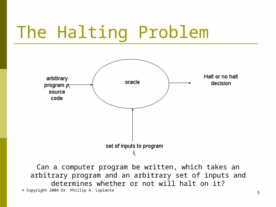
Can a computer program be written, which takes an arbitrary program and an arbitrary set of inputs and determines whether or

not will halt on it?


The Halting Problem

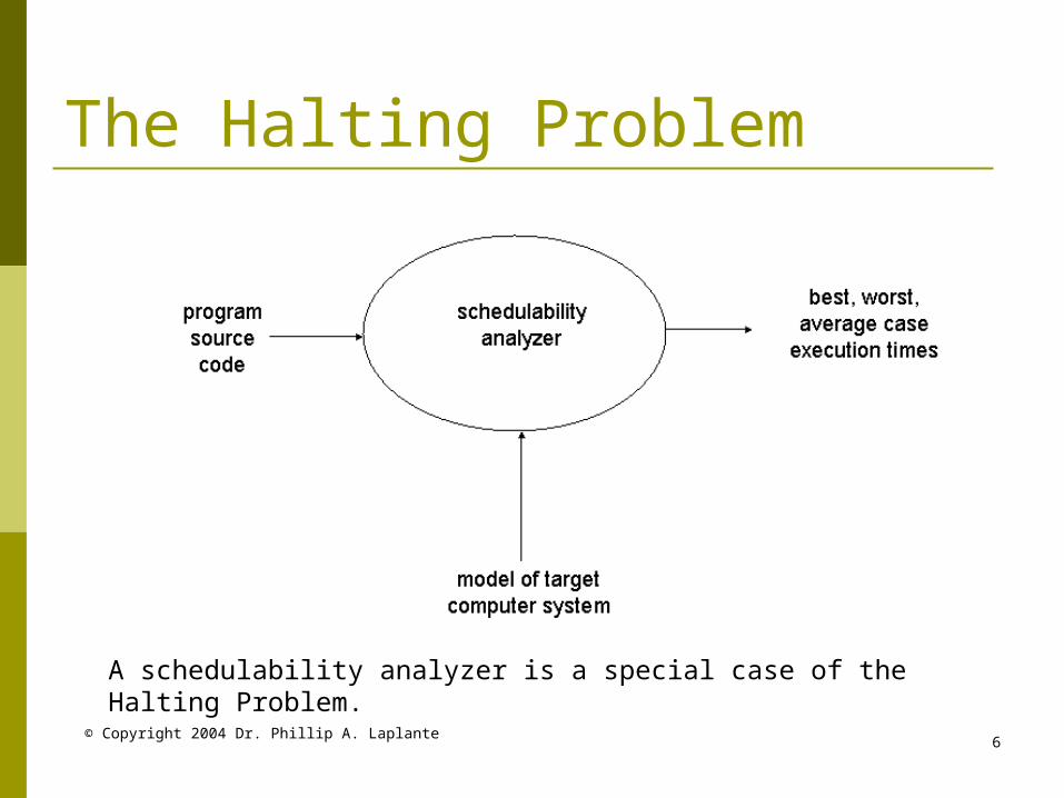
A schedulability analyzer is a special case of the Halting Problem.


Amdahl’s Law Amdahl’s Law – a statement regarding the level

of parallelization that can be achieved by a parallel computer.

Amdahl’s Law – for a constant problem size, speedup approaches zero as the number of processor elements grows.

Amdahl’s Law is frequently cited as an argument against parallel systems and massively parallel processors.

speedup1 ( 1)

n

n s


Gustafson’s Law Gustafson found that the underlying principle that “the

problem size scales with the number of processors” is inappropriate”.

Gustafson’s empirical results demonstrated that the parallel or vector part of a program scales with the problem size.

Times for vector start-up, program loading, serial bottlenecks, and I/O that make up the serial component of the run do not grow with the problem size.

speedup s p n


Gustafson’s Law

0

2

4

6

8

10

12

14

16

18

1 4 7 10 13 16 19 22 25 28 31

Number of Processors

Sp

eed

up

Amdahl

Gustafson

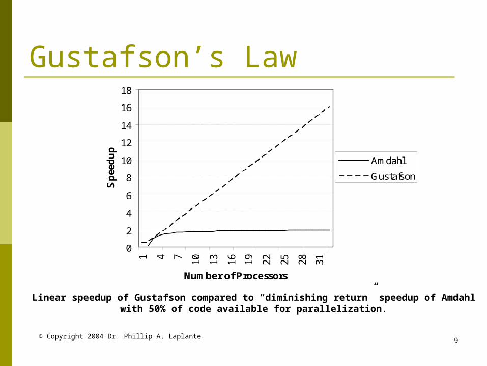
Linear speedup of Gustafson compared to “diminishing return” speedup of Amdahl with 50% of code available for parallelization.


Performance analysis Code execution time estimation Analysis of polled loops Analysis of coroutines Analysis of round-robin systems Response time analysis for fixed period systems Response time analysis -- RMA example Analysis of sporadic and aperiodic interrupt

systems Deterministic performance


Code execution time estimation Instruction counting Instruction execution time simulators Use the system clock


Analysis of polled loops

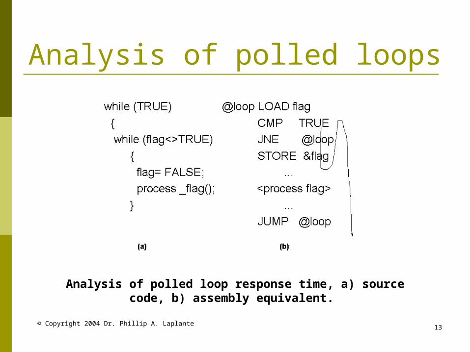
Analysis of polled loop response time, a) source code, b) assembly equivalent.


Analysis of coroutines

Tracing the execution path in a two-task coroutine system. A switch statement in each task drives the phase driven code (not shown). A central dispatcher calls

task1() and task2() and provides intertask communication via global variables or parameter lists.


Analysis of round-robin systems Assume n tasks, each with max execution time c and time

quantum q then T is worst case time from readiness to completion for any task (also known as turnaround time), denoted, is the waiting time plus undisturbed time to complete.

Example, suppose there are 5 processes with a maximum execution time of 500 ms. The time quantum is 100ms. Then total completion time is

( 1)c

T n q cq

500(5 1) 100 500 2500

100T ms


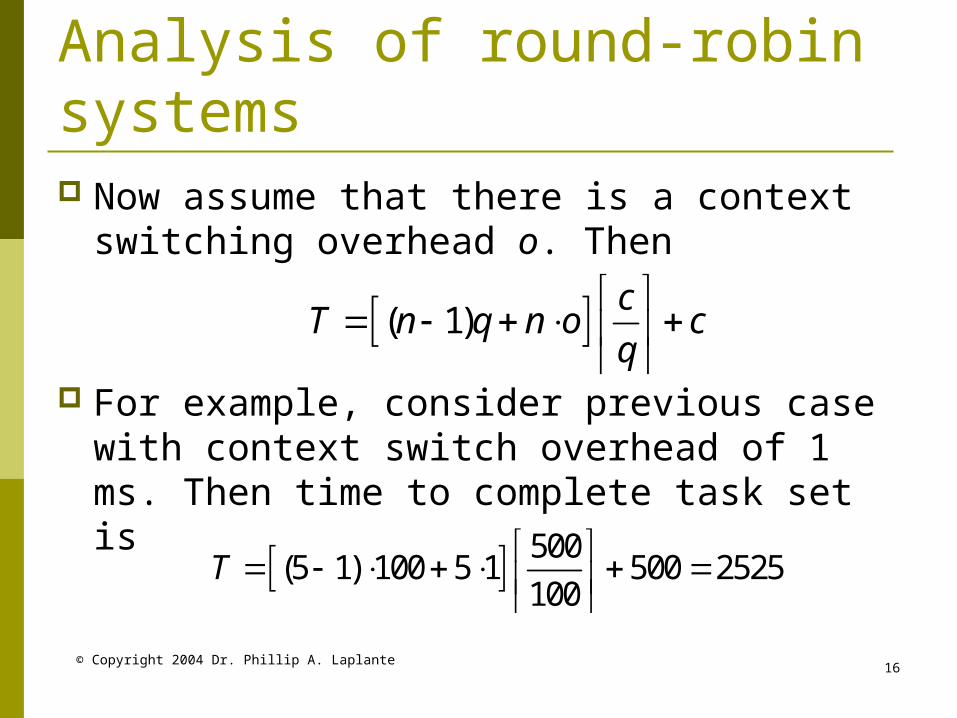
Analysis of round-robin systems Now assume that there is a context

switching overhead o. Then

For example, consider previous case with context switch overhead of 1 ms. Then time to complete task set is

( 1)c

T n q n o cq

500(5 1) 100 5 1 500 2525

100T


Response time analysis for fixed period systems For a general task,response time,Ri,is given as Ri

= ei + Ii where ei is max execution time and Ii is the maximum amount of delay in execution, caused by higher priority tasks.

By solving as a recurrence relation, the response time of the nth iteration can be found as

Where hp(i) is the set tasks of a higher priority than task i.

1

( )

/n ni i i j j

j hp i

R e R p e


Response time analysis for fixed period systems For our purposes, we will only deal with

specific cases of fixed-period systems. Such cases can be handled by manually

constructing a timeline of all tasks and then calculating individual response times directly from the timeline.


Analysis of sporadic and aperiodic interrupt systems Use a rate-monotonic approach with the non-

periodic tasks having a period equal to their worst case expected inter-arrival time.

If this leads to unacceptably high utilizations use a heuristic analysis approach.

Queuing theory can also be helpful in this regard.

Calculating response times for interrupt systems depends on factors such as interrupt latency, scheduling/dispatching times, and context switch times.


Deterministic performance Cache, pipelines, and DMA, all designed to improve average

real-time performance, destroy determinism and thus make prediction of real-time performance troublesome.

To do a worst case performance analysis, assume that every instruction is not fetched from cache but from memory.

In the case of pipelines, always assume that at every possible opportunity the pipeline needs to be flushed.

When DMA is present in the system, assume that cycle stealing is occurring at every opportunity, inflating instruction fetch times.

Does this mean that these make a system effectively unanalyzable for performance? Yes.

By making some reasonable assumptions about the real impact of these effects, some rational approximation of performance is possible.


Application of queuing theory The M/M/1 queue – basic model of a single

server (CPU) queue with exponentially distributed service and inter-arrival times can be used to model interrupt service times and response times.

Little’s law (1961) –Same as utilization calculation!

Erlang’s formula (1917) – can be used to a potential time-overloaded condition.


I/O performance Disk I/O is the single greatest contributor

to performance degradation. It is very difficult to account for disk device

access times when instruction counting. Best approach is to assume worse case

access times for device I/O and include them in performance predictions.


Performance optimization

Compute at slowest cycle Scaled numbers Imprecise computation Optimizing memory usage Post integration software optimization


Compute at slowest cycle All processing should be done at the

slowest rate that can be tolerated. Often moving from fast cycle to slower one

will degrade performance but significantly improve utilization.

For example a compensation routine that takes 20ms in a 40ms cycle contributes 50% to utilization. Moving to 100ms cycle reduces that contribution to only 20%.


Scaled numbers In virtually all computers, integer operations are

faster than floating-point ones. In scaled numbers, the least significant bit (LSB)

of an integer variable is assigned a real number scale factor.

Scaled numbers can be added and subtracted together and multiplied and divided by a constant (but not another scaled number).

The results are converted to floating-point at the last step – hence saving considerable time.


Scaled numbers For example, suppose an analog-to-digital

converter is converting accelerometer data. Let the least significant bit of the two’s

complement 16-bit integer have value 0.0000153 ft/sec2.

Then any acceleration can be represented up to the maximum value of

The 16-bit number 0000 0000 0001 011, for example, represents an acceleration of 0.0001683 ft/sec2.

152 1 *0.0000153 0.5013351


Imprecise computation Sometimes partial results are acceptable in order

to meet a deadline. In the absence of firmware support or DSP

coprocessors, complex algorithms are often employed to produce the desired calculation.

E.g., a Taylor series expansion (perhaps using look-up tables).

Imprecise computation (approximate reasoning) is often difficult to apply because it is hard to determine the processing that can be discarded, and its cost.


Optimizing memory usage In modern computers memory constraints are not

as troublesome as they once were – except in small, embedded, wireless, and ubiquitous computing!

Since there is a fundamental trade-off between memory usage and CPU utilization (with rare exceptions), to optimize for memory usage, trade run-time performance to save memory.

E.g., in look up tables, more entries reduces average execution time and increases accuracy. Less entries saves memory but has reverse effect.

Bottom line: match the real-time processing algorithms to the underlying architecture.


Post integration software optimization After system implementation, techniques can be

used to squeeze additional performance from the machine.

Includes the use of assembly language patches and hand-tuning compiler output.

Can lead to unmaintainable and unreliable code because of poor documentation.

Better to use coding “tricks” that involve direct interaction with the high-level language and that can be documented.

These tricks improve real-time performance, but generally not at the expense of maintainability and reliability.


Results from compiler optimization

use of arithmetic identities reduction in strength common sub-expression

elimination use of intrinsic functions constant folding loop invariant removal loop induction elimination use of revisers and caches dead code removal

flow-of-control optimization constant propagation dead-store elimination dead-variable elimination, short-circuit Boolean code loop unrolling loop jamming cross jump elimination speculative execution

Code optimization techniques used by compilers can be forced manually to improve real-time performance where the compiler does not implement them. These include:


Results from compiler optimization

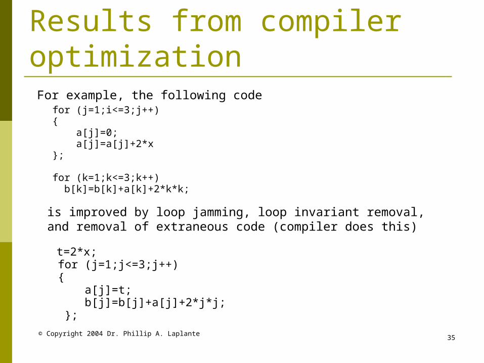
for (j=1;i<=3;j++) { a[j]=0; a[j]=a[j]+2*x }; for (k=1;k<=3;k++) b[k]=b[k]+a[k]+2*k*k;

is improved by loop jamming, loop invariant removal, and removal of extraneous code (compiler does this)

t=2*x; for (j=1;j<=3;j++) { a[j]=t; b[j]=b[j]+a[j]+2*j*j; };

For example, the following code


Results from compiler optimizationNext, loop unrolling yields (you have to do this, not the compiler):

Finally, after constant folding, the improved code is:

t=2*x; a[1]=t ; b[1]=b[1]+a[1]+2*1*1; a[2]=t ; b[2]=b[2]+a[2]+2*2*2; a[3]=t ; b[3]=b[3]+a[3]+2*3*3;

t=2*x; a[1]=t; b[1]=b[1]+a[1]+2; a[2]=t; b[2]=b[2]+a[2]+8; a[3]=t; b[3]=b[3]+a[3]+18;


Results from compiler optimization The original code involved 9 additions and

9 multiplications, numerous data movement instructions, and loop overheads. The improved code requires only 6 additions, 1 multiply, less data movement, and no loop overhead. It is very unlikely that any compiler would have been able to make such an optimization.


Analysis of memory requirements With memory becoming denser and cheaper,

memory utilization analysis has become less of a concern.

Still, its efficient use is important in small embedded systems and air and space applications where savings in size, power consumption, and cost are desirable.

Most critical issue is deterministic prediction of RAM space needed (too little can result in catastrophe).

Same goes for other rewritable memory (e.g. flash memory in Mars Rover).


Reducing memory utilization Shift utilization from one part of memory to

another (e.g. precompute constants and store in ROM).

Reuse variables where possible (document carefully).

Optimizing compilers that manage memory better (e.g. advanced Java memory managers).

Self modifying instructions? Good garbage reclamation and memory

compaction.

© Copyright 2004 Dr. Phillip A. Laplante 1 Performance estimation and optimization Theoretical...

Documents

Transcript of © Copyright 2004 Dr. Phillip A. Laplante 1 Performance estimation and optimization Theoretical...