Analysis of A Single QueueChapter 31

2

Birth Death Processes M/M/1 Queue M/M/m Queue M/M/m/B Queue with Finite Buffers Results for other Queueing systems

Overview

3

Jobs arrive one at a time (and not as a batch)

State = Number of jobs n in the system Arrival of a new job changes the state to

n+1 birth Departure of a job changes the system state

to n-1 death State-transition diagram:

Birth-Death Processes

0 1 2 j-1 j j+1…l0 l1 l2 lj-1 lj lj+1

m1 m2 m3 mj j+1 j+2

4

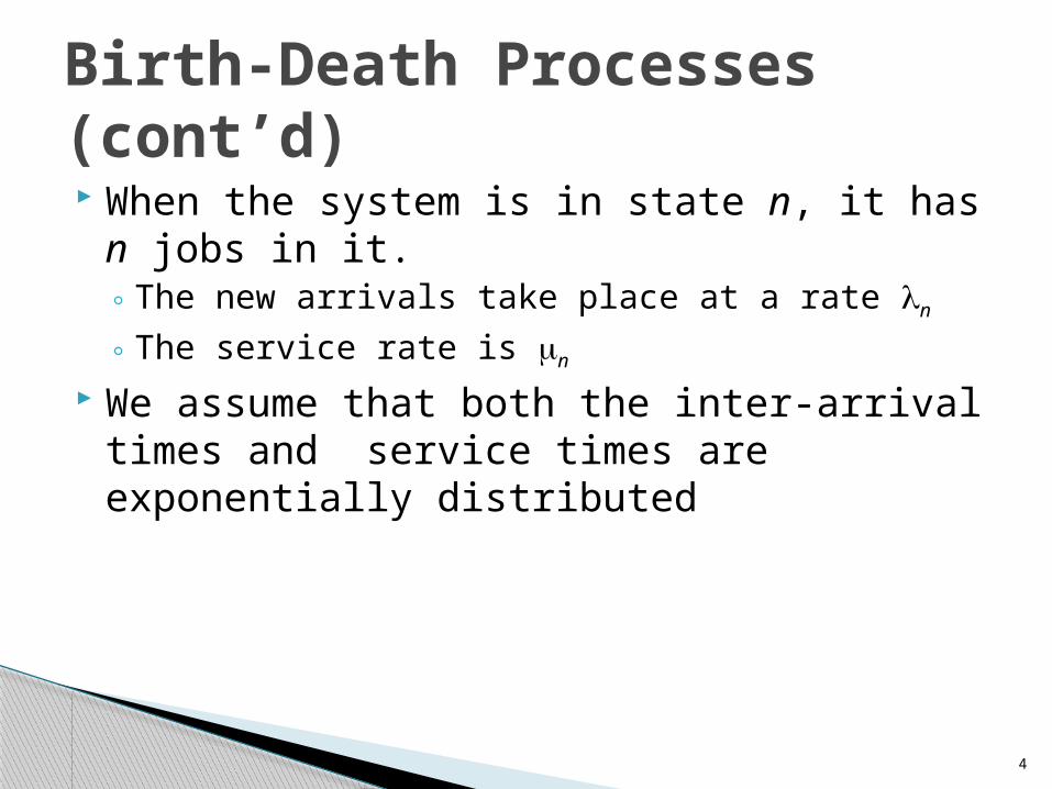
When the system is in state n, it has n jobs in it.◦ The new arrivals take place at a rate ln

◦ The service rate is mn We assume that both the inter-arrival times

and service times are exponentially distributed

Birth-Death Processes (cont’d)

5

The steady-state probability pn of a birth-death process being in state n is given by:

Here, p0 is the probability of being in the zero state

Theorem: State Probability

6

Proof

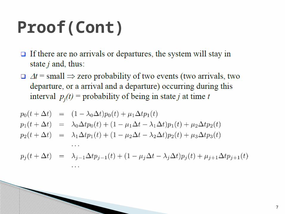
7

Proof(Cont)

8

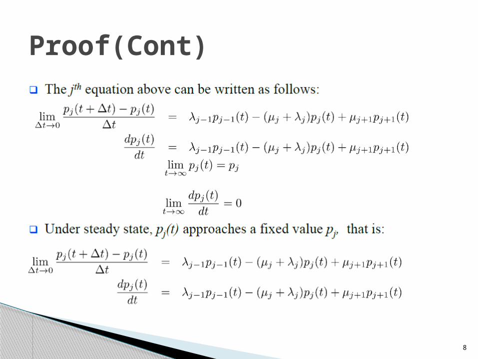
Proof(Cont)

9

Proof(Cont)

10

The sum of all probabilities must be equal to one:

11

M/M/1 queue is the most commonly used type of queue Used to model single processor systems or to model

individual devices in a computer system Assumes that the interarrival times and the service

times are exponentially distributed and there is only one server

No buffer or population size limitations and the service discipline is FCFS

Need to know only the mean arrival rate l and the mean service rate m

State = number of jobs in the system

M/M/1 Queue

0 1 2 J-1 J J+1…l l l l l l

m m m m

12

Results for M/M/1 Queue

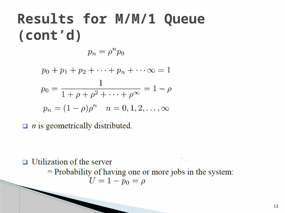
13

Results for M/M/1 Queue (cont’d)

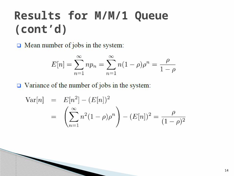
14

Results for M/M/1 Queue (cont’d)

15

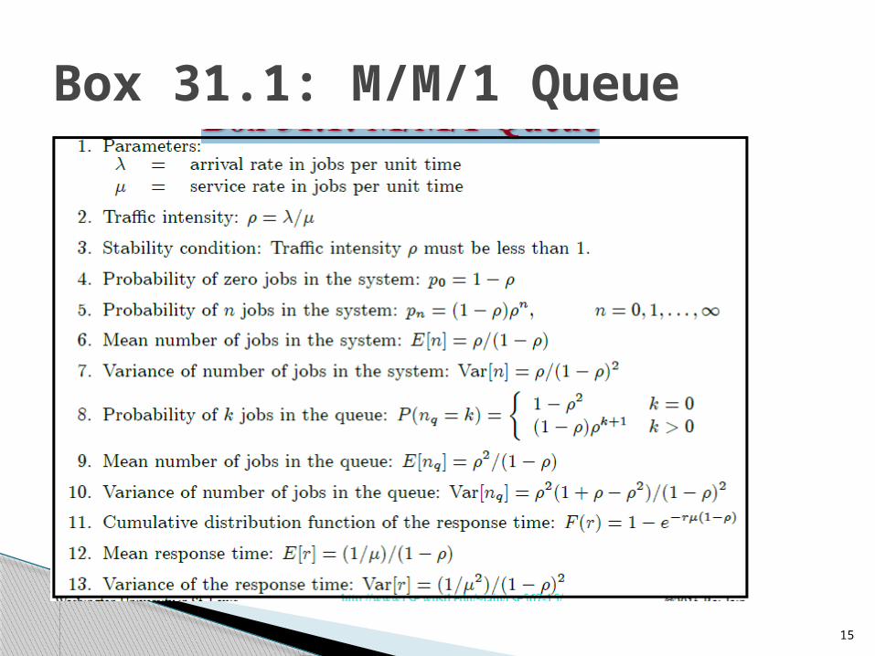
Box 31.1: M/M/1 Queue

16

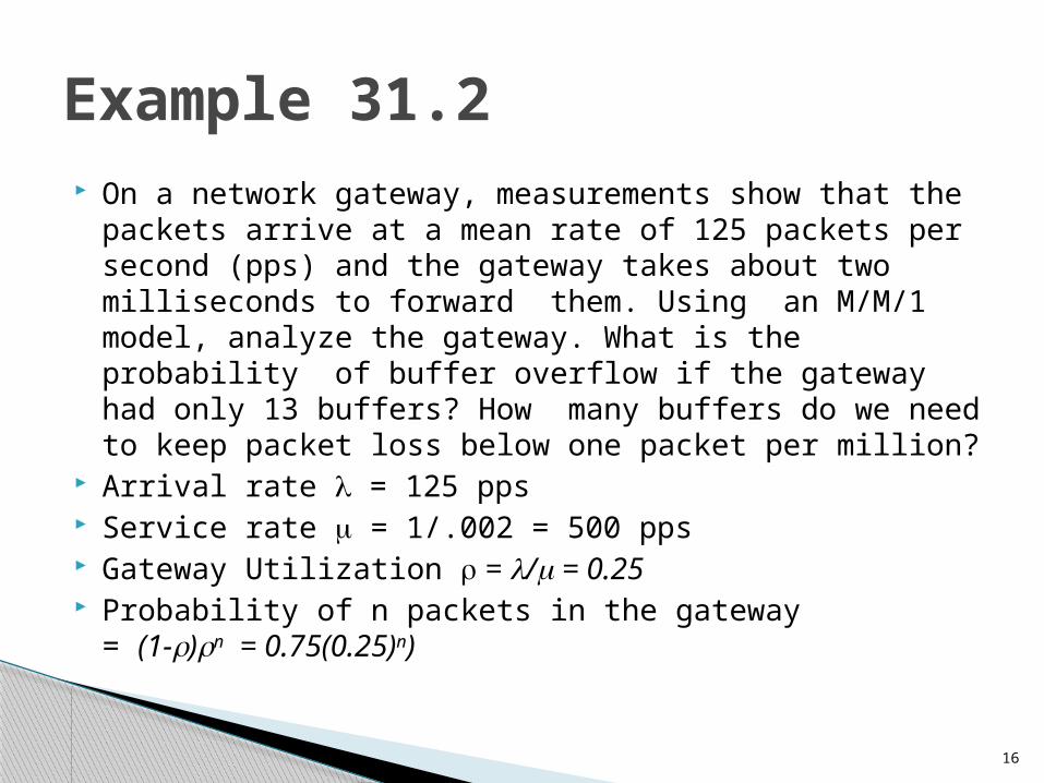
On a network gateway, measurements show that the packets arrive at a mean rate of 125 packets per second (pps) and the gateway takes about two milliseconds to forward them. Using an M/M/1 model, analyze the gateway. What is the probability of buffer overflow if the gateway had only 13 buffers? How many buffers do we need to keep packet loss below one packet per million?

Arrival rate l = 125 pps Service rate m = 1/.002 = 500 pps Gateway Utilization r = l/m = 0.25 Probability of n packets in the gateway

= (1-r)rn = 0.75(0.25)n)

Example 31.2

17

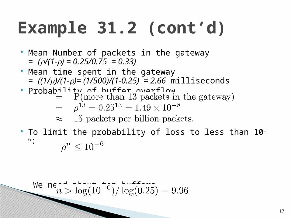
Mean Number of packets in the gateway = (r/(1-r) = 0.25/0.75 = 0.33)

Mean time spent in the gateway = ((1/m)/(1-r)= (1/500)/(1-0.25) = 2.66 milliseconds

Probability of buffer overflow

To limit the probability of loss to less than 10-6:

We need about ten buffers.

Example 31.2 (cont’d)

18

The last two results about buffer overflow are approximate. Strictly speaking, the gateway should actually be modeled as a finite buffer M/M/1/B queue. However, since the utilization is low and the number of buffers is far above the mean queue length, the results obtained are a close approximation.

Example 31.2 (cont’d)

19

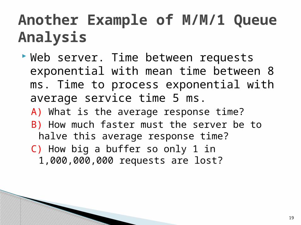
Web server. Time between requests exponential with mean time between 8 ms. Time to process exponential with average service time 5 ms.A) What is the average response time?B) How much faster must the server be to halve

this average response time?C) How big a buffer so only 1 in 1,000,000,000

requests are lost?

Another Example of M/M/1 Queue Analysis

20

Another Example of M/M/1 Queue AnalysisRequest rate

= 1/ 8 = 0.125 requests per ms

Service rate = 1/ 5 = 0.2

requests per msUtilization

= /= .125/.2 = .625So, 62.5% of

capacityA) Avg response time

(1/) / (1-)= (1/.2)/(1-.625)= 13.33 ms

To halve, want(1/) / (1-) = 6.665

Assume fixed, so change

= 1/6.665 + 0.125 = .257

B) So, (.275-.2)/.2 * 100= 37.5% faster

1 in 1 billion errorsBuffer size k:

Pr(k) 10-9

k 10-9

C) So, k > log(10-9) / log(.625)k 44

21

Single Queue, Multiple Servers - M/M/m Queue

22

How does response time for previous M/M/1 Web server change if number of servers increased to 4? ◦ Can model as M/M/4

M/M/m Example

23

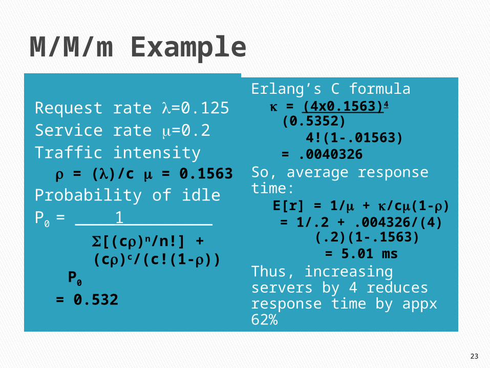
M/M/m Example

Request rate =0.125Service rate =0.2Traffic intensity

= ()/c = 0.1563

Probability of idleP0 = ____1_________

[(c)n/n!] + (c)c/(c!

(1-)) P0

= 0.532

Erlang’s C formula = (4x0.1563)4

(0.5352) 4!(1-.01563)= .0040326

So, average response time:

E[r] = 1/ + /c(1-)= 1/.2 + .004326/(4)

(.2)(1-.1563)= 5.01 ms

Thus, increasing servers by 4 reduces response time by appx 62%

24

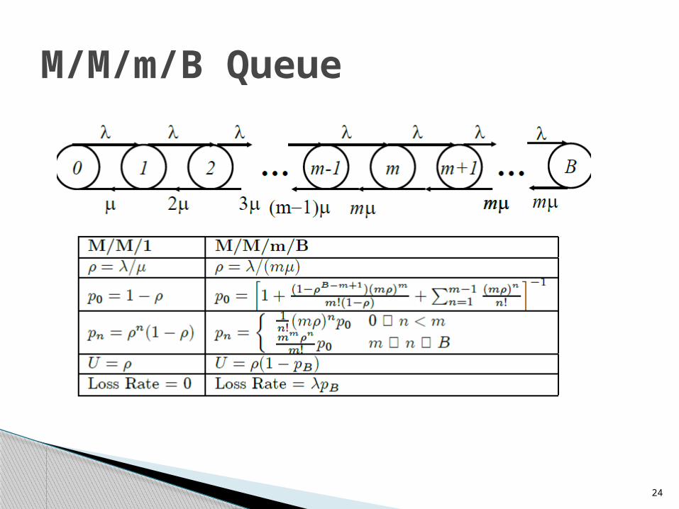
M/M/m/B Queue

25

Birth-death processes: Compute probability of having n jobs in the system

M/M/1 Queue: Load-independent => Arrivals and service do not depend upon the number in the system

Summary