Working.doc - AP Calculus BC
23
Board Approved 8-3-15 1 Curriculum: AP Calculus BC Curricular Unit: Slope Fields; Euler’s Method; Logistic Growth; Improper Integrals; Relative Rates of Growth Instructional Unit: A. Euler’s Method, Differential Equations, Improper Integrals, and Slope Fields – demonstrate knowledge of slope fields, Euler’s Method, differential equations, and improper integrals Description Section in Schoolnet: I.C. Functions, Graphs, and Limits: Asymptotic and Unbounded Behavior 3. Comparing relative magnitudes of functions and their rates of change (For example, contrasting exponential growth, polynomial growth, and logarithmic growth) II.E. Derivatives: Applications of Derivatives 7. Geometric interpretation of differential equations via slope fields and the relationship between slope fields and solution curves for differential equations 8. Numerical solution of differential equations using Euler’s method III.D. Integrals: Techniques of Antidifferentiation 3. Improper integrals (as limits of definite integrals) III.E. Integrals: Applications of Antidifferentiation 2. Solving separable differential equations and using them in modeling 3. Solving logistic differential equations and using them in modeling Standard Alignments (Section 2) GLE/CLE: N/A Knowledge: (MA) 1,2 CCSS: N/A APCALC: BC.Ic.3; BC.IIe.7,8; BC.IIId.3; BC.IIIe.2,3 NETS: 1c; 4c Performance: 1.6, 3.2, 3.6 Unit (Section 3) Learning Targets: • Determine the relative rate of growth for different functions • Evaluate improper integrals to determine if they converge or diverge • Use Euler’s Method to approximate a solution of a differential equation • Solve a differential equation
Transcript of Working.doc - AP Calculus BC
Board Approved 8-3-15
1
Curriculum: AP Calculus BC Curricular Unit: Slope Fields; Euler’s Method; Logistic Growth; Improper Integrals; Relative Rates of Growth Instructional Unit: A. Euler’s Method, Differential Equations, Improper Integrals, and Slope Fields – demonstrate knowledge of slope fields, Euler’s Method, differential equations, and improper integrals Description Section in Schoolnet: I.C. Functions, Graphs, and Limits: Asymptotic and Unbounded Behavior 3. Comparing relative magnitudes of functions and their rates of change
(For example, contrasting exponential growth, polynomial growth, and logarithmic growth)
II.E. Derivatives: Applications of Derivatives 7. Geometric interpretation of differential equations via slope fields and the
relationship between slope fields and solution curves for differential equations
8. Numerical solution of differential equations using Euler’s method III.D. Integrals: Techniques of Antidifferentiation 3. Improper integrals (as limits of definite integrals) III.E. Integrals: Applications of Antidifferentiation 2. Solving separable differential equations and using them in modeling 3. Solving logistic differential equations and using them in modeling
Standard Alignments (Section 2) GLE/CLE: N/A Knowledge: (MA) 1,2 CCSS: N/A APCALC: BC.Ic.3; BC.IIe.7,8; BC.IIId.3; BC.IIIe.2,3 NETS: 1c; 4c Performance: 1.6, 3.2, 3.6
Unit (Section 3)
Learning Targets: • Determine the relative rate of growth for different functions • Evaluate improper integrals to determine if they converge or diverge • Use Euler’s Method to approximate a solution of a differential equation • Solve a differential equation
Board Approved 8-3-15
2
• Interpret differential equations geometrically using slope fields and the relationship between slope fields and solution curves
• Solve a logistic differential equation and interpret the result Instructional Strategies: • Lecture enhanced with:
• SMART Notebook • PowerPoint • the Internet
• Drill and guided practice • Demonstrations • Reflective discussion • Class discussion • Computer assisted instruction • Activity: Spreading a Rumor: Students will collect logistical data by simulating a
rumor spreading by using the random integer generator feature on their graphing calculators
Assessments/Evaluations: • Students will be assessed on the concepts taught using a variety of modalities:
• Direct teacher observations • Formative assessments • Homework assignments • Formal common assessment
Mastery: 80% Sample Assessment Questions: • Ten grizzly bears were introduced into a national park 10 years ago. There are 23
bears in the park at the present time. The park can support a maximum of 100 bears A) Write the differential equation. B) Solve the differential equation. C) Sketch a graph of the solution to the differential equation with labels and a
window. D) How many bears will there be 5 years from now? E) When is the population growing the fastest? When t = _____________ and P =
________________. Instructional Resources/Tools: • Textbook(s): Chapters 7 & 9 - Finney, Ross L., Franklin D. Demana, Bert K. Waits,
and Daniel Kennedy. Calculus: Graphical, Numerical, Algebraic. 4th ed. Boston: Prentice Hall, 2012. Print. APEdition.
• Website(s): http://www.otherwise.com/population/logistic.html • Graphing calculator Cross Curricular Connections: •
Board Approved 8-3-15
3
Depth of Knowledge (Section 5) DOK: 4
Board Approved 8-3-15
4
Curriculum: AP Calculus BC Curricular Unit: Sequences; Series Instructional Unit: B. Introduction to Sequences and Series – use appropriate formulas to calculate terms and sums of sequences and series Description Section in Schoolnet: IV.A. Polynomial Approximations and Series: Concept of a Series: 1. A series is defined as a sequence of partial sums, and convergence is
defined in terms of the limit of the sequence of partial sums. Technology can be used to explore convergence and divergence
IV.B. Polynomial Approximations and Series: Series of constants: 2. Geometric series with applications
Standard Alignments (Section 2) GLE/CLE: N/A Knowledge: (MA) 1,2 CCSS: N/A APCALC: BC.IVa.1; BC.IVb.2 NETS: 6a Performance: 1.6, 3.2, 3.6
Unit (Section 3)
Learning Targets: • Determine if a series or sequence is arithmetic, geometric, or neither and find new
terms • Determine the explicit formula for the nth term of a given series and use it to find
specific terms • Determine the explicit formula for a series written recursively and find new terms • Determine if a geometric series has a limit and use the formula to find the limit • Determine if a sequence has a limit • Expand a series written in ∑ notation • Rewrite an expanded series in ∑ notation • Determine the sum of n terms of a geometric or arithmetic series • Determine if a geometric series has a limit and use the formula to find the limit
Board Approved 8-3-15
5
Instructional Strategies: • Lecture enhanced with:
• SMART Notebook • PowerPoint • the Internet
• Drill and guided practice • Demonstrations • Reflective discussion • Class discussion • Computer assisted instruction • Activity: Objective Review – take a list of objectives that deal with evaluating terms
of sequences and sums of series and compose a problem illustrating each objective Assessments/Evaluations: • Students will be assessed on the concepts taught using a variety of modalities:
• Direct teacher observations • Formative assessments • Homework assignments • Formal common assessment
Mastery: 80% Sample Assessment Questions: • Which is more: being given one million dollars, or one penny the first day, double
that penny the next day, then double the previous day's pennies and so on for 30 days? Show your work using a series to make your decision
Instructional Resources/Tools: • Worksheets developed by the instructor • Graphing calculator Cross Curricular Connections: •
Depth of Knowledge (Section 5) DOK: 4
Board Approved 8-3-15
6
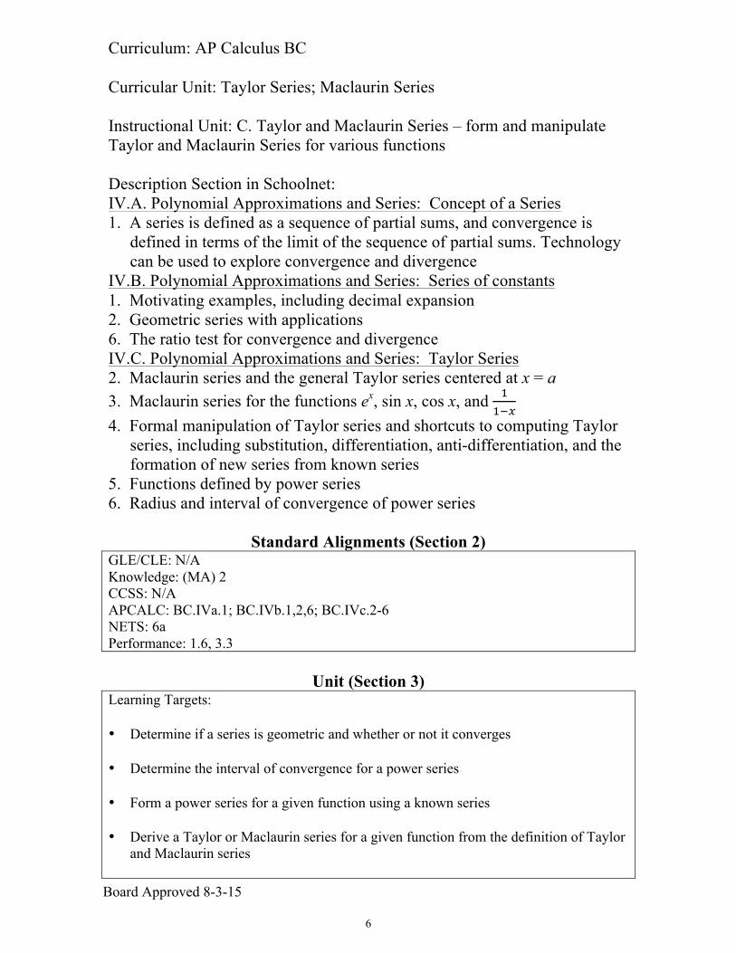
Curriculum: AP Calculus BC Curricular Unit: Taylor Series; Maclaurin Series Instructional Unit: C. Taylor and Maclaurin Series – form and manipulate Taylor and Maclaurin Series for various functions Description Section in Schoolnet: IV.A. Polynomial Approximations and Series: Concept of a Series 1. A series is defined as a sequence of partial sums, and convergence is
defined in terms of the limit of the sequence of partial sums. Technology can be used to explore convergence and divergence
IV.B. Polynomial Approximations and Series: Series of constants 1. Motivating examples, including decimal expansion 2. Geometric series with applications 6. The ratio test for convergence and divergence IV.C. Polynomial Approximations and Series: Taylor Series 2. Maclaurin series and the general Taylor series centered at x = a 3. Maclaurin series for the functions ex, sin x, cos x, and !
!!!
4. Formal manipulation of Taylor series and shortcuts to computing Taylor series, including substitution, differentiation, anti-differentiation, and the formation of new series from known series
5. Functions defined by power series 6. Radius and interval of convergence of power series
Standard Alignments (Section 2) GLE/CLE: N/A Knowledge: (MA) 2 CCSS: N/A APCALC: BC.IVa.1; BC.IVb.1,2,6; BC.IVc.2-6 NETS: 6a Performance: 1.6, 3.3
Unit (Section 3)
Learning Targets: • Determine if a series is geometric and whether or not it converges • Determine the interval of convergence for a power series • Form a power series for a given function using a known series • Derive a Taylor or Maclaurin series for a given function from the definition of Taylor
and Maclaurin series

Board Approved 8-3-15
7
• Know from memory the Taylor or Maclaurin Series for ex,!sin x,!cos x,!ln x and 11! x
• Determine if a sequence converges or diverges and find the limit as n→∞ if it exists (limits you should know)
• Use the ratio test to determine the open interval and radius of convergence for a
power series Instructional Strategies: • Lecture enhanced with:
• SMART Notebook • PowerPoint • the Internet
• Drill and guided practice • Demonstrations • Reflective discussion • Class discussion • Computer assisted instruction • Activity: Illustrate a converging series on graph paper – Students will use graph paper
to illustrate the series !!+ !
!+ !
!… and investigate whether it converges or diverges
Assessments/Evaluations: • Students will be assessed on the concepts taught using a variety of modalities:
• Direct teacher observations • Formative assessments • Homework assignments • Formal common assessment
Mastery: 80% Sample Assessment Questions: • KNOWN SERIES: Find a Power series representation for f (x) = x2 cos(3x) using a
known series. Write in ∑ notation, as well as writing the 1st three nonzero terms. • Derive from the definition of Maclaurin Series the infinite series for e5x. Show at least
3 terms and ∑ notation. • Use the ratio test to prove that the Maclaurin Series for sin x converges for all x. Instructional Resources/Tools: • Textbook(s): Chapters 9 & 10 - Finney, Ross L., Franklin D. Demana, Bert K. Waits,
and Daniel Kennedy. Calculus: Graphical, Numerical, Algebraic. 4th ed. Boston: Prentice Hall, 2012. Print. APEdition.
• Graphing calculator Cross Curricular Connections: •
Depth of Knowledge (Section 5) DOK: 4
Board Approved 8-3-15
8
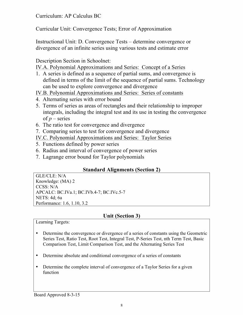
Curriculum: AP Calculus BC Curricular Unit: Convergence Tests; Error of Approximation Instructional Unit: D. Convergence Tests – determine convergence or divergence of an infinite series using various tests and estimate error Description Section in Schoolnet: IV.A. Polynomial Approximations and Series: Concept of a Series 1. A series is defined as a sequence of partial sums, and convergence is
defined in terms of the limit of the sequence of partial sums. Technology can be used to explore convergence and divergence
IV.B. Polynomial Approximations and Series: Series of constants 4. Alternating series with error bound 5. Terms of series as areas of rectangles and their relationship to improper
integrals, including the integral test and its use in testing the convergence of p – series
6. The ratio test for convergence and divergence 7. Comparing series to test for convergence and divergence IV.C. Polynomial Approximations and Series: Taylor Series 5. Functions defined by power series 6. Radius and interval of convergence of power series 7. Lagrange error bound for Taylor polynomials
Standard Alignments (Section 2) GLE/CLE: N/A Knowledge: (MA) 2 CCSS: N/A APCALC: BC.IVa.1; BC.IVb.4-7; BC.IVc.5-7 NETS: 4d; 6a Performance: 1.6, 1.10, 3.2
Unit (Section 3)
Learning Targets: • Determine the convergence or divergence of a series of constants using the Geometric
Series Test, Ratio Test, Root Test, Integral Test, P-Series Test, nth Term Test, Basic Comparison Test, Limit Comparison Test, and the Alternating Series Test
• Determine absolute and conditional convergence of a series of constants • Determine the complete interval of convergence of a Taylor Series for a given
function
Board Approved 8-3-15
9
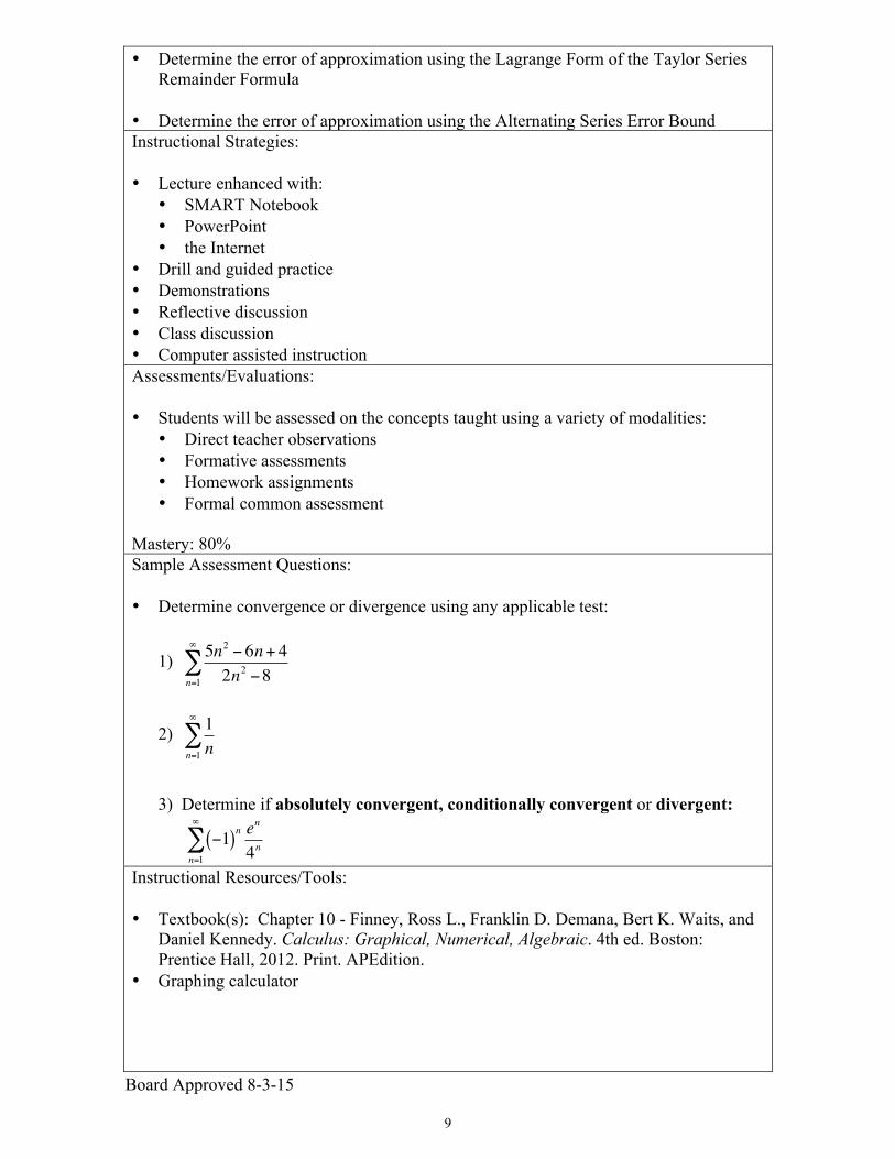
• Determine the error of approximation using the Lagrange Form of the Taylor Series Remainder Formula
• Determine the error of approximation using the Alternating Series Error Bound Instructional Strategies: • Lecture enhanced with:
• SMART Notebook • PowerPoint • the Internet
• Drill and guided practice • Demonstrations • Reflective discussion • Class discussion • Computer assisted instruction Assessments/Evaluations: • Students will be assessed on the concepts taught using a variety of modalities:
• Direct teacher observations • Formative assessments • Homework assignments • Formal common assessment
Mastery: 80% Sample Assessment Questions: • Determine convergence or divergence using any applicable test:
1) 5n2 ! 6n+ 42n2 !8n=1
"
#
2) 1nn=1
!
"
3) Determine if absolutely convergent, conditionally convergent or divergent:
!1( )n en
4nn=1
"
#
Instructional Resources/Tools: • Textbook(s): Chapter 10 - Finney, Ross L., Franklin D. Demana, Bert K. Waits, and
Daniel Kennedy. Calculus: Graphical, Numerical, Algebraic. 4th ed. Boston: Prentice Hall, 2012. Print. APEdition.
• Graphing calculator
Board Approved 8-3-15
10
Cross Curricular Connections: •
Depth of Knowledge (Section 5) DOK: 4
Board Approved 8-3-15
11
Curriculum: AP Calculus BC Curricular Unit: Parametric Equations Instructional Unit: E. Parametric Equations – utilize parametric forms of equations Description Section in Schoolnet: I.A. Functions, Graphs, and Limits: Analysis of Graphs 1. With the aid technology, graphs of functions are often easy to produce.
The emphasis is on the interplay between the geometric and analytic information and on the use of calculus both to predict and to explain the observed local and global behavior of a function
I.E. Parametric, Polar, and Vector Functions 1. The analysis of planar curves includes those given in parametric form,
polar form, and vector form II.B. Derivative at a Point 1. Slope of a curve at a point. Examples are emphasized, including points at
which there are vertical tangents and points at which there are no tangents
2. Tangent line to a curve at a point and local linear approximation II.E. Applications of Derivatives 2. Analysis of planar curves given in parametric form, polar form, and
vector form, including velocity and acceleration II.F. Computation of Derivatives 4. Derivatives of parametric, polar, and vector functions III.B. Applications of Integrals 1. Appropriate integrals are used in variety of applications to model
physical, biological, or economic situations. To provide a common foundation, specific applications should include the length of a curve given in parametric form
Standard Alignments (Section 2)
GLE/CLE: N/A Knowledge: (MA) 2,4 CCSS: N/A APCALC: BC.Ia.1; BC.Ie.1; BC.IIb.1,2; BC.IIe.2; BC.IIf.4; BC.IIIb.1 NETS: 1c; 6a Performance: 1.6, 1.10, 3.2
Board Approved 8-3-15
12
Unit (Section 3) Learning Targets: • Show a complete parametric graph on the calculator and identify the initial point,
terminal point, and direction of motion on the graph • Convert equations from parametric to Cartesian by eliminating the parameters • Write a set of parametric equations to represent a conic section • Solve application problems involving motion using parametric equations • Find derivatives of functions given in parametric form • Write the equation of a tangent line using parametric equations • Find arc length of a curve given by parametric equations • Identify points on a curve where vertical and horizontal tangents occur • Find the area of a surface of revolution defined by parametric equations Instructional Strategies: • Lecture enhanced with:
• SMART Notebook • PowerPoint • the Internet
• Drill and guided practice • Demonstrations • Reflective discussion • Class discussion • Computer assisted instruction • Activity: Parametric Fun – Students graph parametric equations to explore the effect
of parameter changes Assessments/Evaluations: • Students will be assessed on the concepts taught using a variety of modalities:
• Direct teacher observations • Formative assessments • Homework assignments • Formal common assessment
Mastery: 80%
Board Approved 8-3-15
13
Sample Assessment Questions: • It’s the bottom of the ninth inning, the Cardinals are behind 6-3 and the bases are
loaded. Stan Musial is at bat. He swings and makes contact with the ball 3 feet above the plate at an angle of 20 degrees from the horizontal at a velocity of 150 feet per second. He hits straight toward center field where there is a fence 400 feet from home plate and 20 feet high. At the moment the ball is hit, there is a wind blowing straight in from center field at 6 miles per hour (8.8 feet per second). Does Stan hit a grand slam and win the game? 1) Write and graph the parametric equations describing the following situations:
a) the two equations representing the path of the ball if there were no wind b) the two equations representing a wind of 6 miles per hour c) the two equations representing a wind of 12 miles per hour
2) Decide if any of the above would result in a home run. 3) Decide which is a more important factor: velocity or angle. Explain your choice
with specific numerical examples using the above equations for a foundation. Use different values for angle and velocity in your determination. Take into account real-world issues of factors that affect velocity and angle
Instructional Resources/Tools: • Textbook(s): Chapter 11 - Finney, Ross L., Franklin D. Demana, Bert K. Waits, and
Daniel Kennedy. Calculus: Graphical, Numerical, Algebraic. 4th ed. Boston: Prentice Hall, 2012. Print. APEdition.
• Graphing calculator Cross Curricular Connections: •
Depth of Knowledge (Section 5) DOK: 4
Board Approved 8-3-15
14
Curriculum: AP Calculus BC Curricular Unit: Polar Equations Instructional Unit: F. Polar Equations – utilize polar forms of equations Description Section in Schoolnet: I.A. Functions, Graphs, and Limits: Analysis of Graphs 1. With the aid technology, graphs of functions are often easy to produce.
The emphasis is on the interplay between the geometric and analytic information and on the use of calculus both to predict and to explain the observed local and global behavior of a function.
I.E. Parametric, Polar, and Vector Functions 1. The analysis of planar curves includes those given in parametric form,
polar form, and vector form II.B. Derivative at a Point 1. Slope of a curve at a point. Examples are emphasized, including points at
which there are vertical tangents and points at which there are no tangents
2. Tangent line to a curve at a point and local linear approximation II.E. Applications of Derivatives 2. Analysis of planar curves given in parametric form, polar form, and
vector form, including velocity and acceleration II.F. Computation of Derivatives 4. Derivatives of parametric, polar, and vector functions III.B. Applications of Integrals 1. Appropriate integrals are used in variety of applications to model
physical, biological, or economic situations. To provide a common foundation, specific applications should include the length of a curve given in parametric form
Standard Alignments (Section 2)
GLE/CLE: N/A Knowledge: (MA) 2,4 CCSS: N/A APCALC: BC.Ia.1; BC.Ie.1; BC.IIb.1,2; BC.IIe.2; BC.IIf.4; BC.IIIb.1 NETS: 1c; 6a Performance: 1.6, 1.10, 3.2
Unit (Section 3)
Learning Targets: • Graph points on polar paper
Board Approved 8-3-15
15
• Convert coordinates from rectangular to polar and vice versa • Find other possible sets of polar coordinates for a given point • Convert equations in rectangular form to polar form and vice versa • Graph polar equations by hand using a t-table • Identify types of polar graphs given an equation • Find the derivative of a polar equation • Find arc length of a given polar equation • Find area of a polar region • Find intersection points of polar equations • Find area of intersecting polar curves Instructional Strategies: • Lecture enhanced with:
• SMART Notebook • PowerPoint • the Internet
• Drill and guided practice • Demonstrations • Reflective discussion • Class discussion • Computer assisted instruction • Activity: On-line Interactive Polar Graphing game Assessments/Evaluations: • Students will be assessed on the concepts taught using a variety of modalities:
• Direct teacher observations • Formative assessments • Homework assignments • Formal common assessment
Mastery: 80% Sample Assessment Questions: • Consider the polar curve r = 2sin 3!( ) for 0 !! ! " .
a) In the xy–plane provided, sketch the curve. b) Find the area of the region inside the curve.
c) Find the slope of the curve at the point where ! = "4
Board Approved 8-3-15
16
Instructional Resources/Tools: • Textbook(s): Chapter 11 - Finney, Ross L., Franklin D. Demana, Bert K. Waits, and
Daniel Kennedy. Calculus: Graphical, Numerical, Algebraic. 4th ed. Boston: Prentice Hall, 2012. Print. APEdition.
• Graphing calculator Cross Curricular Connections: •
Depth of Knowledge (Section 5) DOK: 4
Board Approved 8-3-15
17
Curriculum: AP Calculus BC Curricular Unit: Calculus of Vector Functions Instructional Unit: G. Calculus of vector functions – apply concepts of calculus to vector defined functions Description Section in Schoolnet: I.A. Functions, Graphs, and Limits: Analysis of Graphs 1. With the aid technology, graphs of functions are often easy to produce.
The emphasis is on the interplay between the geometric and analytic information and on the use of calculus both to predict and to explain the observed local and global behavior of a function
I.E. Functions, Graphs, and Limits: Parametric, Polar, and Vector Functions 1. The analysis of planar curves includes those given in parametric form,
polar form, and vector form II.B. Derivatives: Derivative at a Point 1. Slope of a curve at a point. Examples are emphasized, including points at
which there are vertical tangents and points at which there are no tangents
2. Tangent line to a curve at a point and local linear approximation II.E. Derivatives: Applications of Derivatives 2. Analysis of planar curves given in parametric form, polar form, and
vector form, including velocity and acceleration II.F. 4. Derivatives of parametric, polar, and vector functions
Standard Alignments (Section 2) GLE/CLE: N/A Knowledge: (MA) 2,3 CCSS: N/A APCALC: BC.Ia.1; BC.Ie.1; BC.IIb1,2; BC.IIe.2; BC.IIf.4 NETS: 4d; 6b,d Performance: 1.6, 1.10, 3.2, 3.6
Unit (Section 3)
Learning Targets: • Name and define vectors • Find the magnitude of a given vector • Perform arithmetic operations on vectors, both algebraically and geometrically • Find the resultant vector using scalar multiplication and scalar addition
Board Approved 8-3-15
18
• Find components of a vector given the initial and terminal points • Find a unit vector in the same direction of a given vector • Find limits of vector-valued functions • Calculate and graph a vector value function • Find the unit tangent vector at a point and the equations of the corresponding tangent
and normal lines • Find direction of motion using a vector value function • Apply concepts of displacement, distance, velocity, acceleration, and speed to vector
– valued functions using derivatives and integrals Instructional Strategies: • Lecture enhanced with:
• SMART Notebook • PowerPoint • the Internet
• Drill and guided practice • Demonstrations • Reflective discussion • Class discussion • Computer assisted instruction Assessments/Evaluations: • Students will be assessed on the concepts taught using a variety of modalities:
• Direct teacher observations • Projects w/ scoring guides: AP Packet – students will complete problems from
previous Advanced Placement exams that pertain to vectors and use the scoring guides provided by the College Board to examine their solutions for correctness
• Quiz • Homework assignments • Formal common assessment
Mastery: 80% Sample Assessment Questions: • An object moving along a curve in the xy-plane has position (x(t), y(t)) at time t with
dxdt= cos t3( )!!and !!dydt = 3sin t2( )
for 0 < t < 3. At time t = 2, the object is at position (4, 5). a) Write an equation for the line tangent to the curve at (4,5) b) Find the speed of the object at time t = 2. c) Find the total distance traveled by the object of the time interval 0 < t < 1. d) Find the position of the object at time t = 3.
Board Approved 8-3-15
19
Instructional Resources/Tools: • Textbook(s): Chapter 11 - Finney, Ross L., Franklin D. Demana, Bert K. Waits, and
Daniel Kennedy. Calculus: Graphical, Numerical, Algebraic. 4th ed. Boston: Prentice Hall, 2012. Print. APEdition.
• Website(s): Introduction to Vector: • http://www.youtube.com/watch?v=ajTeseYcimE • http://www.livebinders.com/play/play/538864
• Graphing calculator Cross Curricular Connections: •
Depth of Knowledge (Section 5) DOK: 4
Board Approved 8-3-15
20
Curriculum: AP Calculus BC Curricular Unit: Working AP Problems Instructional Unit: H. Solve AP Problems – demonstrate knowledge of calculus by solving a variety of AP style problems Description Section in Schoolnet: I. Functions, Graphs, and Limits II. Derivatives III. Integrals IV. Polynomial Approximations and Series
Standard Alignments (Section 2) GLE/CLE: N/A Knowledge: (MA) 2,3 CCSS: N/A APCALC: BC.Ia-e; BC.IIa-f; BC.IVa-f; BC.IIIa-c (Concepts only) NETS: 4d; 6b,d Performance: 1.6, 1.10, 3.2, 3.6
Unit (Section 3)
Learning Targets: • Solve problems similar to those found on AP Calculus AB and/or BC exams Instructional Strategies: • Lecture enhanced with: • SMART Notebook • PowerPoint • the Internet • Drill and guided practice • Demonstrations • Reflective discussion • Class discussion • Computer assisted instruction • One or more of the following hands-on activities:
• AP Calculus Jeopardy game • AP Calculus Clue game • Calculus Murder Mystery • Interactive online calculus computer game (written by instructor)
Board Approved 8-3-15
21
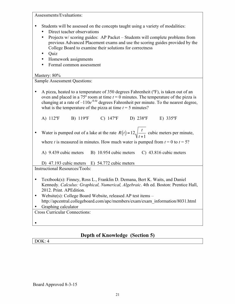
Assessments/Evaluations: • Students will be assessed on the concepts taught using a variety of modalities:
• Direct teacher observations • Projects w/ scoring guides: AP Packet – Students will complete problems from
previous Advanced Placement exams and use the scoring guides provided by the College Board to examine their solutions for correctness
• Quiz • Homework assignments • Formal common assessment
Mastery: 80% Sample Assessment Questions: • A pizza, heated to a temperature of 350 degrees Fahrenheit (ºF), is taken out of an
oven and placed in a 75º room at time t = 0 minutes. The temperature of the pizza is changing at a rate of –110e-0.4t degrees Fahrenheit per minute. To the nearest degree, what is the temperature of the pizza at time t = 5 minutes? A) 112ºF B) 119ºF C) 147ºF D) 238ºF E) 335ºF
• Water is pumped out of a lake at the rate R t( ) =12 tt +1
cubic meters per minute,
where t is measured in minutes. How much water is pumped from t = 0 to t = 5?
A) 9.439 cubic meters B) 10.954 cubic meters C) 43.816 cubic meters D) 47.193 cubic meters E) 54.772 cubic meters
Instructional Resources/Tools: • Textbook(s): Finney, Ross L., Franklin D. Demana, Bert K. Waits, and Daniel
Kennedy. Calculus: Graphical, Numerical, Algebraic. 4th ed. Boston: Prentice Hall, 2012. Print. APEdition.
• Website(s): College Board Website, released AP test items – http://apcentral.collegeboard.com/apc/members/exam/exam_information/8031.html
• Graphing calculator Cross Curricular Connections: •
Depth of Knowledge (Section 5) DOK: 4
Board Approved 8-3-15
22
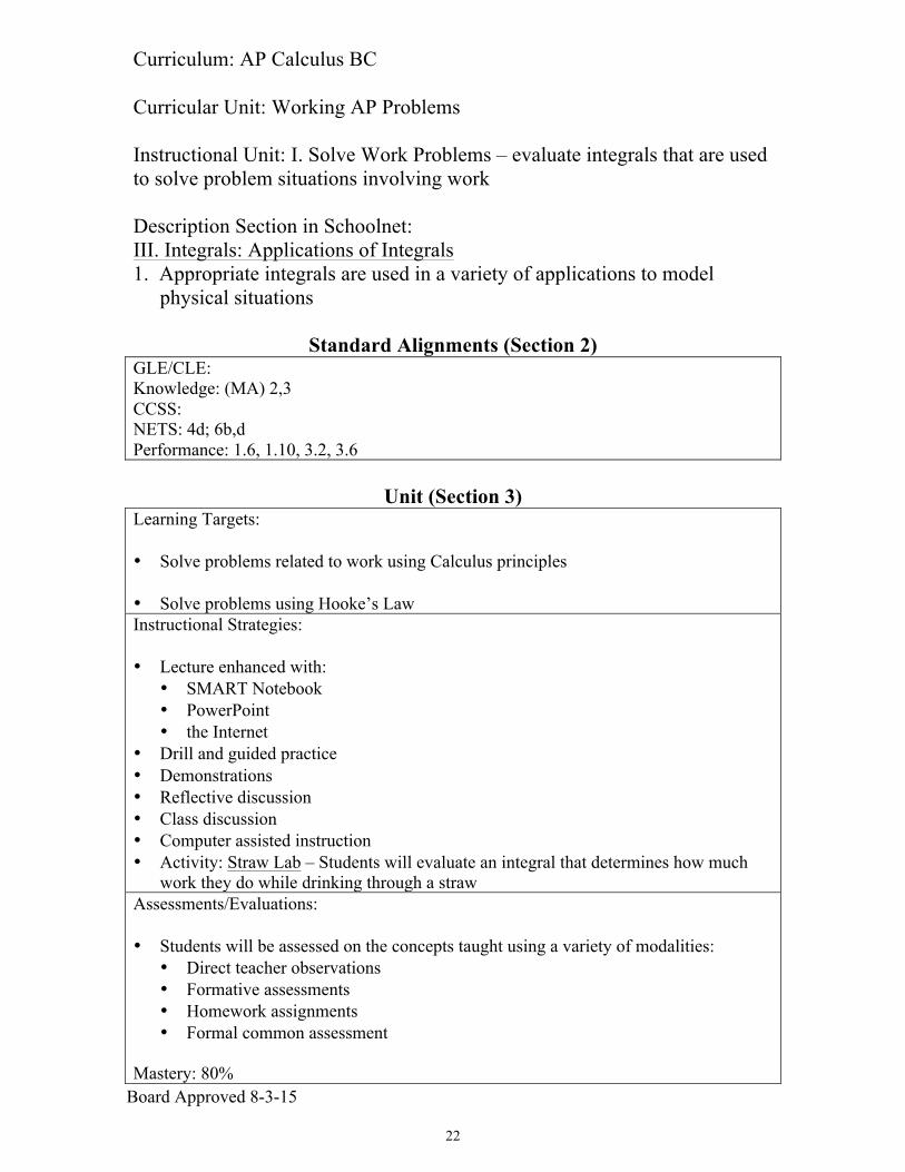
Curriculum: AP Calculus BC Curricular Unit: Working AP Problems Instructional Unit: I. Solve Work Problems – evaluate integrals that are used to solve problem situations involving work Description Section in Schoolnet: III. Integrals: Applications of Integrals 1. Appropriate integrals are used in a variety of applications to model
physical situations
Standard Alignments (Section 2) GLE/CLE: Knowledge: (MA) 2,3 CCSS: NETS: 4d; 6b,d Performance: 1.6, 1.10, 3.2, 3.6
Unit (Section 3)
Learning Targets: • Solve problems related to work using Calculus principles • Solve problems using Hooke’s Law Instructional Strategies: • Lecture enhanced with:
• SMART Notebook • PowerPoint • the Internet
• Drill and guided practice • Demonstrations • Reflective discussion • Class discussion • Computer assisted instruction • Activity: Straw Lab – Students will evaluate an integral that determines how much
work they do while drinking through a straw Assessments/Evaluations: • Students will be assessed on the concepts taught using a variety of modalities:
• Direct teacher observations • Formative assessments • Homework assignments • Formal common assessment
Mastery: 80%
Board Approved 8-3-15
23
Sample Assessment Questions: • Find the work done in pushing a car a distance of 30 feet along a level road while
exerting a constant force of 95 pounds. • A rocket on the launch pad weighs 40 tons. By the time it reaches an altitude of 80
miles, it weighs only 10 tons because 30 tons of fuel has been used. Assume the weight of the rocket decreases linearly with displacement above the earth. How many mile-tons of work are done in lifting the rocket to an altitude of 80 miles?
• A force of 9 pounds is required to stretch a spring from its natural length of 6 inches to a length of 8 inches. Find the work done in stretching the spring: a) from its natural length to a length of 10 inches. b) from a length of 7 inches to a length of 9 inches. c) compressing it from its natural length to 2 inches smaller.
Instructional Resources/Tools: • Textbook(s): Chapter 8 - Finney, Ross L., Franklin D. Demana, Bert K. Waits, and
Daniel Kennedy. Calculus: Graphical, Numerical, Algebraic. 4th ed. Boston: Prentice Hall, 2012. Print. APEdition.
• Website(s): Hooke’s Law – http://webphysics.davidson.edu/applets/animator4/demo_hook.html
• Graphing calculator Cross Curricular Connections: •
Depth of Knowledge (Section 5) DOK: 4