CTA 2013 Torino - Sessione speciale sulla Robustezza Strutturale

AAllmmaa MMaatteerr SSttuuddiioorruumm –– UUnniivveerrssiittàà ddii BBoollooggnnaa
DOTTORATO DI RICERCA IN
INGEGNERIA STRUTTURALE ED IDRAULICA
Ciclo XXIII
Settore scientifico-disciplinare di afferenza: ICAR09
Fiber beam-columns models with flexure-shear interaction for nonlinear analysis of reinforced concrete structures.
Presentata da: Filippo Cardinetti Coordinatore Dottorato Relatore Chiar.mo Prof. Erasmo Viola Chiar.mo Prof. Pier Paolo Diotallevi Correlatore
Ing. Luca Landi
Esame finale anno 2011

Abstract
The aim of this study was to develop a model capable to capture the different contributions
which characterize the nonlinear behaviour of reinforced concrete structures. In particular,
especially for non slender structures, the contribution to the nonlinear deformation due to
bending may be not sufficient to determine the structural response. Two different models
characterized by a fibre beam-column element are here proposed. These models can
reproduce the flexure-shear interaction in the nonlinear range, with the purpose to improve
the analysis in shear-critical structures. The first element discussed is based on flexibility
formulation which is associated with the Modified Compression Field Theory as material
constitutive law. The other model described in this thesis is based on a three-field
variational formulation which is associated with a 3D generalized plastic-damage model as
constitutive relationship.
The first model proposed in this thesis was developed trying to combine a fibre beam-
column element based on the flexibility formulation with the MCFT theory as constitutive
relationship. The flexibility formulation, in fact, seems to be particularly effective for
analysis in the nonlinear field. Just the coupling between the fibre element to model the
structure and the shear panel to model the individual fibres allows to describe the nonlinear
response associated to flexure and shear, and especially their interaction in the nonlinear
field. The model was implemented in an original matlab® computer code, for describing
the response of generic structures. The simulations carried out allowed to verify the field of
working of the model. Comparisons with available experimental results related to
reinforced concrete shears wall were performed in order to validate the model. These
results are characterized by the peculiarity of distinguishing the different contributions due
to flexure and shear separately. The presented simulations were carried out, in particular,
for monotonic loading. The model was tested also through numerical comparisons with

Abstract
other computer programs. Finally it was applied for performing a numerical study on the
influence of the nonlinear shear response for non slender reinforced concrete (RC)
members.
Another approach to the problem has been studied during a period of research at the
University of California Berkeley. The beam formulation follows the assumptions of the
Timoshenko shear beam theory for the displacement field, and uses a three-field
variational formulation in the derivation of the element response. A generalized plasticity
model is implemented for structural steel and a 3D plastic-damage model is used for the
simulation of concrete. The transverse normal stress is used to satisfy the transverse
equilibrium equations of at each control section, this criterion is also used for the
condensation of degrees of freedom from the 3D constitutive material to a beam element.
In this thesis is presented the beam formulation and the constitutive relationships, different
analysis and comparisons are still carrying out between the two model presented.

Table of contents
Chapter 1 - Inroduction
1.1 Sommario 1
1.2 Different approaches to the nonlinear analyses of reinforced concrete structures 1
1.2.1 Macroscopic approach 1
1.2.2 Microscopic approach 2
1.2.3 Global models 3
1.2.4 Fibre Models 10
1.3 Aim and objective of the thesis 13
1.4 Outline of the thesis 14
Chapter 2 - Fibre beam-column element with flexure-shear interaction: state of
the art
2.1 Sommario 16
2.2 Fibre Beam‐Column Element Using Strut‐and‐Tie Models 17
2.2.1 Guedes’s Model 17
2.2.2 Martinelli’s Model 20
2.2.3 Ranzo and Petrangeli’s model 23
2.3 Fibre Beam‐Column Element Using Microplane Model 27
2.3.1 Petrangeli’s Model 27
2.4 Fibre Beam‐Column Element Using Smeared Crack Models 29

2.4.1 Vecchio and Collins’s model 29
2.4.2 Bentz’s Model 33
2.4.3 Remino’ Model. 35
2.4.4 Bairan’s Model 37
2.5 Fibre Beam‐Column Element Using Damage Models. 41
2.5.1 Modello di Mazars 41
Chapter 3 - Fibre beam-column beam formulation
3.1 Sommario 44
3.2 Definition of the vectors involved 45
3.3 Formulation of the element starting from mixed method 46
3.4 Element state determination 48
3.4.1 Description of the procedure 49
3.4.2 Element state determination algorithm. 50
Chapter 4 - Constitutive Relationship: Section state determination
4.1 Sommario 55
4.2 Modified compression field theory 56
4.2.1 Introduction 56
4.2.2 Compatibility condition 56
4.2.3 Equilibrium Condition 57
4.2.4 Constitutive relationship 59
4.2.5 Transmitting loads across the cracks 60
4.3 Disturbed stress field model 63

4.3.1 General overview 64
4.3.2 Equilibrium equation 65
4.3.3 Compatibility relations 67
4.3.4 Constitutive Relations 69
4.3.5 Shear slip model 71
Chapter 5 - Implementation of the model
5.1 Sommario 74
5.2 Definition input vectors and matrices 75
5.3 Algorithm steps 77
5.3.1 Structure state determination 80
5.3.2 Element state determination 81
5.3.3 Section state determination 83
5.4 Solution strategies 89
5.5 Flow Chart 91
5.5.1 Structure state determination 91
5.5.2 Element state determination 92
5.5.3 Section state determination 93
Chapter6 - Numerical analysis and validation
6.1 Sommario 97
6.2 Comparisons between numerical and experimental results 98
6.2.1 Geometry of specimen B4 and modeling criteria 98
6.2.2 Results of the comparison 101

6.3 Numerical comparison with VecTor2 106
6.4 Investigation on the influence of flexure‐shear interaction 107
6.4.1 Parametric analysis on bridge pier 107
6.4.2 Parametric analysis on a shear wall 111
6.4.3 Analysis with the ratio (slender shear wall) L/D=10. 111
6.4.4 Analysis with the ratio L/D=2 . 116
6.4.5 Analysis with the ratio L/D=1. 118
Chapter 7 - Alternative formulation for the shear critical beam-column element
(developed in University of California Berkeley)
7.1 Sommario 121
7.2 Finite element formulation 122
7.2.1 Kinematic assumptions 122
7.2.2 Hu‐Washizu Functional 122
7.2.3 Force interpolation matrix 126
7.2.4 Descripion of the shear forces 126
7.2.5 Section deformation and stiffness matrix 127
7.3 Constitutive relationships. 128
7.3.1 Steel material model 128
7.3.2 Concrete material model 130
Conclusion 134
References 137

CHAPTER 1
Introduction
1.1 Sommario
In questo capitolo introduttivo verranno trattati i criteri di modellazione della risposta
sismica non lineare di strutture in c.a. Si riporta sia una classificazione delle diverse
tipologie di modelli, sia una descrizione degli aspetti che sono stati sviluppati e
perfezionati nel corso degli ultimi decenni. Vengono poi richiamati alcuni modelli e, senza
entrare nel dettaglio, se non evidenziando le caratteristiche salienti. In questo modo è
possibile inquadrare meglio le proprietà e le assunzioni su cui si basano i modelli proposti.
1.2 Different approaches to nonlinear analysis of reinforced concrete
structures
The study of reinforced concrete structures under strong seismic actions requires the
formulation of analytical models capable of describing the behaviour of structural elements
subject to cyclic loading in the non-linear fields, taking into account the typical phenomena
of progressive deterioration of stiffness and strength. the following approaches can be
distinguished in relation to the complexity and the model scale.
1.2.1 Macroscopic approach
Structural modeling of the is made trying to achieve a correspondence between the
structural members and the elements of the analytical model. To this end, the one-
dimensional elements are used to simulate the response of a beam, columns, or a wall
portion between two floors. Following a macroscopic approach the effects of geometry
details can be lost, such as the exact form of longitudinal and transverse reinforcement, but
the main aspects of structural behavior can be reproduced quickly and the spread inelastic
deformations along the element can be considered.
A typical example of the macroscopic approach are the global models. The constitutive
laws for this kind of modes, are introduced in terms of section forces-section deformation
such as moment-curvature relations. These approximation are sufficiently accurate to
describe the aspects that characterize the cyclic loading response, defined through

CHAPTER 1
2
hysteretic model. The reduced computational time and accurate simulation of the global
hysteretic behavior, makes these models the most efficient method for the analysis of
complex structures, consisting in a large number of elements.
The class of fiber models can be set in a macroscopic approach, indeed each structural
element can be described by a single finite element, and the equilibrium and compatibility
conditions are expressed in global terms. The sections behavior is studied through a
discretization into finite areas, or, for planar elements, in strips. The constitutive
relationships are locally defined, in terms of stress-strain relation for each fiber. Therefore,
the fiber models are considered as intermediate between local and global formulation. At
one side fiber model are based on simplified kinematic assumptions that allow to reduce
the number of equations, to the other hand the global behaviour is derived from the
materials constitutive laws. However fiber models requires remarkable computational
effort, especially in complex structures analysis.
1.2.2 Microscopic approach
The structure is discretized with a large number of two or three-dimensional finite
elements, using different elements for concrete, reinforcement and the bonds between the
two materials. It’s much more accurate in describing the local behavior, but requires an
excessive computational time. The use of microscopic models allows, at the most, to run
analysis of individual elements or portions of structures, such as walls, beam-column or
nodes.
Introduction
3
1.2.3 Global models
The modeling of seismic behavior of reinforced concrete structures in the last forty years'
was the focus of many researchers and led to the development of multiple types of global
models. Since the late 60s were proposed simple models, which over the years have been
improved and expanded.
This introduction it is focused on the elements for non linear analysis of structures, in
which the shear strength is enough to ensure the development of inelastic deformation. In
this context, global models can be classified in relation to the inelastic deformation
distribution, with this criteria may have lumped plasticity elements and distributed
plasticity elements.
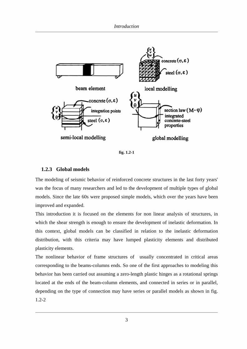
The nonlinear behavior of frame structures of usually concentrated in critical areas
corresponding to the beams-columns ends. So one of the first approaches to modeling this
behavior has been carried out assuming a zero-length plastic hinges as a rotational springs
located at the ends of the beam-column elements, and connected in series or in parallel,
depending on the type of connection may have series or parallel models as shown in fig.
1.2-2
fig. 1.2-1
CHAPTER 1
4
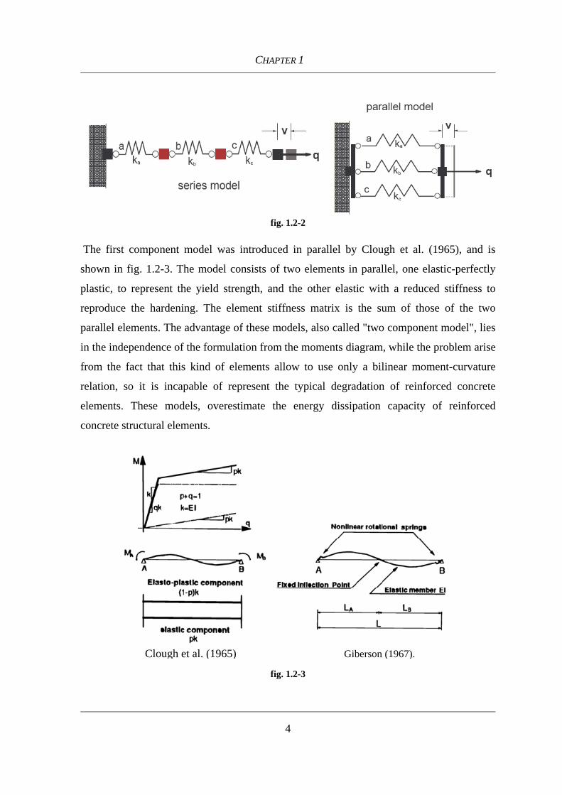
The first component model was introduced in parallel by Clough et al. (1965), and is
shown in fig. 1.2-3. The model consists of two elements in parallel, one elastic-perfectly
plastic, to represent the yield strength, and the other elastic with a reduced stiffness to
reproduce the hardening. The element stiffness matrix is the sum of those of the two
parallel elements. The advantage of these models, also called "two component model", lies
in the independence of the formulation from the moments diagram, while the problem arise
from the fact that this kind of elements allow to use only a bilinear moment-curvature
relation, so it is incapable of represent the typical degradation of reinforced concrete
elements. These models, overestimate the energy dissipation capacity of reinforced
concrete structural elements.
fig. 1.2-2
Clough et al. (1965) Giberson (1967).
fig. 1.2-3

Introduction
5
Series models were introduced to overcoming the limitations inherent in the parallel
models. They were formally introduced by Giberson (1967), the model (fig. 1.2-3) consists
of two non-linear rotational springs and end of an elastic beam. For each spring is
introduced a moment-rotation relationship assuming an antisymmetric linear distribution of
moments along the element. In series models the flexibility matrix of each spring is
summed with the flexibility matrix of the linear elastic beam. This type of models are
much more versatile than the parallels, with series models is possible to describe a more
complex hysteretic behavior, selecting an appropriate moment-rotation relationship for
springs, but they are limited by the assumption of a constant moments distribution along
the element. Suko and Adams (1971), proposed to take the contraflexure point from the
initial elastic analysis instead of the center of the beam. Otani (1974), proposed a more
sophisticated model, shown in fig. 1.2-4. The Otani’s model consists of two deformable
parallel elements, one linear elastic and the other non-linear, two rotational springs and two
rigid connection at the ends to take into account the finite size of the beam-column node.
The rotational springs are used to consider the effects of the reinforcement slip at the
nodes. The construction of the flexibility matrix is based on the calculation of the
contraflexure point step by step. The element is treated as two cantiliver beams, with a free
end at the contraflexure point. With this assumption the element is equivalent to two
inelastic rotational springs at the ends, whose properties are related to the current position
of the contraflexure point. The Otani’s model, however, is not capable to evaluate the
actual spread inelasticity along the element, depending not only on the current state of the
element, but also on the load history.

CHAPTER 1
6
Concentrated plasticity models have been formulated neglecting the phenomena of axial
force-moment interaction. The moment-rotation relationship are defined referring to a
constant value of axial force, usually the gravity loads. Actually, the normal stress in the
columns due to seismic action can vary significantly, affecting both the resistance and the
stiffness properties of structural elements. Considerable efforts have been made to include
the effects induced by the variations of normal stress in simplified models, but this kind of
models are not applied extensively. Saatcioglu et al. (1983) introduced a concentrated
plasticity model, in which the moment-rotation relationship of the springs is characterized
by a family of curves, each corresponding to a different value of normal stress.
An important step in the modeling of axial force-bending moment interaction, was made
with the introduction of multispring models, which are classified between as concentrated
plasticity, but actually these differ considerably from those described above, and in
somehow are similar to simplified fibers models. The first multispring model was proposed
by Lai et al. (1984), it was constituted by a central elastic element, and a series of axial
springs at the end zones to simulate the inelastic response (fig. 1.2-5). The non-linear
deformations are concentrated in the end zone, although their behavior is not defined by
fig. 1.2-4

Introduction
7
the moment-rotation relation, but through a discretization of such zones in areas that
represent the springs.
In the Lai’s model each inelastic element consists of five spring for concrete, four for
corners and a central one, and four for steel. The force-displacement relationship for the
steel springs follows an hysteretic model with degradation similar to that assumed on the
moment-rotation relationship viewed for others concentrated plasticity models. The
elongation of each spring is correlated with the average axial displacement and the section
rotation, through the assumption of plane sections remain plain.
Saiid et al. (1989), proposed a multispring model with five springs based on Lai et al.
(1984). One spring is central to simulate concrete core, while four springs are placed at
sides to simulate the behavior of a reinforced concrete element subjected to axial
elongation, corresponding to the area represented by each spring. With this model the
authors overcame some inherent inconsistencies in the Lai’s model, and have performed
good comparison with experimental tests.
The best feature of multispring models is the ability to simulate with good accuracy the
nonlinear behavior of spatial columns, requiring much lower computational effort than
fiber models.
fig. 1.2-5

CHAPTER 1
8
The concentrated plasticity models, as seen above, are not able to take into account the
gradual spread of inelastic deformation within the elements. A more accurate description
of the nonlinear behavior of reinforced concrete elements is possible by using distributed
plasticity models. These kind of models assumes that the inelastic deformation may occur
in any section, the element response is derived through an integration of sections response
along the element.
Schnobrich and Takayanagi (1979), have proposed to divide the element into a finite
number of segments (fig. 1.2-6), each with constant properties dependent on the bending
moment at the midpoint. Each segment is studied through a moment-curvature relation
including the effects of degradation due to cyclic loading. Also in this model a proposal to
take account the axial-bending interaction is made. The section stiffness is defined,
including axial effects, as resulting from predefined interaction diagrams.
Analyze the sections response along the element leads to various difficulties, for the
greatest calculation time and for the numerical problems related to the arise of unbalanced
moments within the element. Equilibrate these moments requires the introduction of
complex procedures not necessary when are studied only the end sections. Therefore,
several authors have developed concentrated plasticity models able to take into account the
gradual spread inelasticity. These models, also called distributed inelasticity have been
widely used, and many computer codes have been based on them.
In fig. 1.2-6 is shown the Meyer’s model, Meyer et al. (1983) and the later one improved
by Roufaiel and Meyer (1987). The element is divided into three zones, one central elastic
and two inelastic ends, varying in length depending on the load history.

Introduction
9
This formulation is independent from the position of contraflexure point, and take into
account the coupling of the inelastic deformation in the two non linear segments. The
properties of these segment are derived by simplified assumptions on the end sections,
carried out through hysteretic moment-curvature models
Schnobrich and Keshavarzian (1985), have adopted the same element, but taking into
account axial-flexure interaction. To consider these effects they followed a similar
approach to that proposed by Takayanagi and Schnobrich (1979).
The criteria used by Meyer et al. (1983) is part of the formulation of Filippou and Issa
(1988), and Mulas and Filippou (1990), which added to the element, two rotational springs
at the extremities, for take into account the fixed end rotation at the beam-column joint,
due to bar pull-out.effects. These authors have attempted to define more accurately the
moment-rotation relationship of the springs, which was independent from the assumed
moment-curvature relationship at the end sections. Filippou Ambrisi (1997) have included
more non-linear springs to account for translational non-linear deformations due to shear.
This model is made up of several sub-elements connected in series to distinguish the
various aspects that affect the nonlinear behavior of the structural element.
A further evolution was carried out by Aredia and Pinto (1998) dividing the element into
three zones. They have developed a method to identify, in the elastic part of the element,
cracked and uncracked zones. Their model is based on the assumption that the elastic limit
Schnobrich and Takayanagi (1979) Roufaiel e Meyer (1987).
fig. 1.2-6

CHAPTER 1
10
may be exceeded only in the end zone, and that the cracked areas can be developed at both
of them, both from the central section of the element, where it is possible to apply a
concentrated load. Both areas, cracked and plasticized have variable length depending on
the loading history, determined by taking a linear progression of bending moment from
each end to the center of the beam.
A common plasticity model that differs from those just described was carried out by
Kunnath et al. (1990), this model can perform local and global damage evaluation as well
as non-linear seismic analysis of reinforced concrete structures. Kunnath et al. (1990) did
not directly assess the length of the plasticized hinges. The element characteristics will be
deducted from the sections by integration, assuming a flexibility distribution piecewise
linear (fig. 1.2-7) .
This distribution is identified by the beam ends flexibility, that come from the moment-
curvature relationship, and from the flexibility of the contraflexure point, which is assumed
to be equal to the elastic value.
1.2.4 Fibre Models
In Fibres models is carried out a double discretization, in the longitudinal direction
difining a predetermined number of sections and in the transverse direction, discretizing in
small finite areas the element cross sections. In case of simple planar bending model is
sufficient to subdivide the sections into strips perpendicular to the axis of flexion, in the
more general spatial cases a double subdivision into small rectangular areas is required
fig. 1.2-7

Introduction
11
(fig. 1.2-8). Each fiber, represent a corresponding portion of elementary concrete or
reinforcement area , by integration over the cross section is possible to obtain moment-
curvature relationship, and thus determines the overall response of the whole element. By
the hypothesis of plane sections remain plane, axial deformation of each fiber ( , )x yε can
be obtained, once knowing curvature xχ , yχ and axial deformation 0ε referred in section
centroid.
0( , ) z xx y y zε ε χ χ= + ⋅ − ⋅ (1.3.1)
The characteristics described above are common to all models, so that not changes in
different element formulations. What really change in different fibre models is essentially
the state determination procedures that depend on different formulation. In fact fiber
models, as distributed plasticity models, has the problem, highlighted in previous
paragraph, about the arise of unbalanced section forces within the element. After a load
step application, nodal displacement are calculated and from these the section forces can be
evaluated, but because of the materials nonlinear behavior in all control sections, resisting
forces doesn’t match section forces.
fig. 1.2-8
CHAPTER 1
12
In global models, especially those with concentrated plasticity this problem is not treated
because only the end sections are taken into account. Fibre models differ therefore in the
process used to determine the section resisting forces. Different procedure has been
proposed depending on the element formulation, in particular can be found procedure for
stiffness based, flexibility based or mixed elements.
The early models have been developed on a stiffness based approach, using classical shape
functions. A model that use this approach is due to Aktan et al. (1974), in which nodal
resisting forces are obtained directly from section resisting forces by applying the virtual
work principle. The formulation is compatible, however, it is shown that is inadequate in
nonlinear cases because it involves a linear curvature distribution over the length. This
assumption is unrealistic for reinforced concrete elements in nonlinear field.
The latter models become increasingly based on a flexibility approach, this class of
models uses forces interpolation functions, thus a balanced element is achieved while in
stiffness models the compatibility was the basic assumption. One of the first balanced
element is proposed by Kaba and Mahin (1984), based on Aktan (1974), this model
introduce the displacements interpolation functions updated for each load increment
through the flexibility matrix. In this model, however, the numerical problems discussed
above have not been solved because the theoretical formulation is not totally consistent
with the flexibility approach.
Essentially the flexibility approach is more realistic than the stiffness based one, but
involves significant problems in determining the nodal resisting forces. Many studies,
therefore, have attempted over the years to overcome these problems. Zeris and Mahin
(1988, 1991), developed a complex iterative procedure to investigate the cross section
deformation associated with internal balanced forces, with a shape coincident with forces
interpolation functions. Taucer et al. (1991) have proposed a model that is part of a more
general mixed approach. The nodal resisting forces are calculated for each element through
an iterative procedure. At each iteration, are calculated the residual nodal displacements
associated with the unbalance section forces along the element. The main characteristic of
this model is that, at each iteration, compatibility and equilibrium are satisfied within the
element. Taucer et al. (1991) show that the proposed algorithm is effective even if the
structural response is characterized by "softening" as in concrete structures.

Introduction
13
Finally some recent developments in fiber models are oriented in the attempts to develop
extensions in classical elements including other sources of nonlinear deformation, such as
those related to shear stress. In this class of models, widely described in chapter two, the
section state deformation is characterized not only by the axial deformation and the
curvature in the centroid, but also by the shear deformation evaluated in nonlinear field.
Besides the hypothesis of plane sections remain plane, a given distribution of shear
deformation is assigned in order to detect the state of deformation of each fiber. Generally
a biaxial stress-strain relationships is associated to these elements. This model is very close
to a microscopic approach, but compared to the that has the same degrees of freedom of
beam element type.
In conclusion, fibre models requires a large number of operations to evaluate the element
stiffness matrix, the stress and strain state in each section. In other words fibre models are
really time consuming in state determination procedures. Although sometimes it incurs in
numerical stability problems, many advantages can be identified using these models as:
Catch the actual evolution of plasticization along the element
Are able to reproduce realistically pinching phenomena
Describe in detail geometry and position of transverse reinforcement
Can reproduce the interaction between axial forces and bending moments
Can be easily implemented spatial elements.
Also the constitutive relationship are more easy to implement because the singles materials
are considered instead of moment-curvature relationship.
In this thesis a fibre model able to take into account the coupling between moment, axial
forces, and shear in non-linear field is presented. It is based on the flexibility approach to
take advantage of the benefits attributed to this class of fiber model, in particular between
all fibre modes has been chosen Taucher et all. (1991) because it seemed to respond better
to requests features.
1.3 Aim and objectives of the thesis
The main purpose of the thesis is to propose a finite element able to model structures,
where the shear deformation appears predominant. The category of models chosen to attain
this goal are the fiber models, treated in the previous chapter. As highlighted in the

CHAPTER 1
14
overview in this introduction, the shear deformation and in particular the shear-flexure
coupling in nonlinear field is still an open research topic, in particular, in global models as
beam-column elements.
This aim will be achieved through the following enabling objective:
To gather information on existing knowledge about flexure- shear interaction in
fibres models, through a comprehensive literature review.
To develop and implement an efficient fibre model, capable of predicting the
behaviour of concrete squat structures, which include a bidimensional theory for
concrete (Modified Compression Field Theory) as constitutive relationship.
To validate the model by comparing the predicted behaviour with the behaviour
observed in experimental results, in particular the model must reproduce the global
response of the structure with reasonable agreement with experimental evidence.
To validate the model by comparing the results with another code with different
approach and carrying out a parametric analysis with the aim of study the influence
of flexure-shear interaction by varying the slenderness.
To illustrate a different model proposed, based on a different formulation and a
different constitutive relationship , with the aim of proposing an alternative model
with which, will carry out future comparison and mutual improvement.
1.4 Outline of the thesis
The contents of the thesis will be divided into different chapters as follows:
The first chapter is introductory, recalls some basic concepts of nonlinear analysis and
models categories. In this chapter can be found descriptions of concentrated plasticity
elements (one component and two components model) , distributed plasticity elements
and fibres models, focusing on the stiffness and flexibility formulations highlighting
the benefits and the deficiency of each approach.
The second chapter is entirely dedicated to the state of the art of fibres beam-column
element, in which some author tried to introduce shear deformation. In this chapter will
be discussed in detail each of these models, from the strut and ties, to Microplane and
smeared crack to finish with damage models.

Introduction
15
In the third chapter will be treated the finite element formulation, will be described in
detail the derivation of the flexibility based element, starting from the two-fields mixed
method. This chapter describes how numerical procedures for structural and element
determination have been carried out.
The fourth chapter is entirely dedicated to section state determination, through the
description of MCFT (modified compression field theory) and DSFM (distrurbed
stress field model) that are the basis of the constitutive law implemented in the model.
For each theory will be analyzed compatibility, equilibrium and constitutive
relationships for the average quantities between the material cracks, will be explained
the equilibrium problem on cracks location and shear slip over the cracks.
In the fifth chapter will be explained the implementation of the model, this chapter will
show the vectors and matrices involved in the program and the flow charts of the code.
Furthermore will be explained in detail how the theories on which the model have been
based are unified in a single computer code.
The sixth chapter will report all tests and comparisons performed with the computer
code. First of all will be presented the reproduction of the experimental test conducted
by Osterele et al. (1979). Then will be shown the numerical comparison between the
computer program Vector2, developed at University of Toronto, and the code proposed
in this thesis. Finally, two parametric analysis conducted on a bridge pier and on a
shear wall, show how the nonlinear flexure-shear interaction actually affect the
response in squat structure. Different analysis are carried out with the aim of evaluate
this influence varying the structural slenderness.
The seventh chapter describe the formulation the constitutive relation and the
implementation of the model studied at University of California Berkeley. This model
represent an alternative solution to the presented problem, some comparison between
the two models are in progress. For the element formulation has been used a three-
field variational formulation while for constitutive relationship a three-dimensional
material model. For concrete has been implemented a damage model with two
parameters, one for tension and one for compression Lee and Fenves (1998), while for
steel structures has been implemented a classical plasticity model.

CHAPTER 2
Fibre beam-column element with flexure-shear interaction:
state of the art
2.1 Sommario
Tra i vari approcci adottati per eseguire delle analisi non lineari di strutture in c.a. gli
elementi a fibre hanno mostrato una grande capacità di riprodurre l’interazione tra sforzo
assiale e momento flettente, mentre l’accoppiamento di sforzi normali, flessionali e
taglianti è un fenomeno ancora poco chiaro.
La soluzione al problema della modellazione taglio-flessione è stata affrontata in molti
studi con approcci diversi. Un aspetto che caratterizza molti dei modelli proposti è il
disaccoppiamento di flessione e taglio. Ad esempio, nei modelli “strut and tie” il classico
elemento trave è associato ad un traliccio che simula il meccanismo resistente a taglio. In
alcuni casi i modelli “strut and tie” sono stati combinati con elementi a fibre, come nei
modelli proposti dalla Guedes e Pinto (1997), Martinelli (2002) e da Ranzo e Petrangeli
(1998). Un altro metodo seguito per predire la risposta taglio-flessione si basa sulla teoria
Microplane studiato da Bazant e Oh (1998), Bazant e Prat (1998) e da Bazant e Ozbolt
(1990). L'approccio Microplane permette la descrizione della risposta multiassiale
attraverso la combinazione di relazioni costitutive monoassiali. Petrangeli et al. (1999)
usarono la teoria Microplane all'interno di un elemento a fibre.
Un altro approccio si basa sui modelli a fessurazione diffusa Vecchio e Collins (1988). In
questo approccio, il calcestruzzo fessurato è modellato come un materiale ortotropo, in cui
equilibrio e di compatibilità sono formulati in termini medi di tensione e deformazione..
Remino (2004) ha sviluppato un elemento a fibre con un legame costitutivo basato su Rose
(2001). Ceresa et al. (2008) hanno realizzato un modello a fibre basato su una
formulazione in rigidezze considerando la modified compression field theory (Vecchio e
Collins (1996)) come legame costitutivo. Una particolare tipologia di modelli, come quella
presentata da Mazars et al. (2006), implementano anche la teoria del danno.
In questo capitolo saranno illustrati nel dettaglio questi modelli sottolineandone le
caratteristiche ed i punti deboli.

Fibre beam-column element with flexure-shear interaction: state of the art
17
2.2 Fibre Beam-Column Element Using Strut-and-Tie Models
This approach considers a Timoshenko fibre beam-column element, which is coupled with
a truss structure. All the shear action is carried by the truss members. There are several
models that adopt this technique, these models are presented below.
2.2.1 Guedes’s Model
Guedes et. al. (1994-1997) proposed a two-node 3D beam-column element based on a
displacement formulation, with linear shape functions for axial displacement and rotation.
The degrees of freedom per node are six, three displacements and three rotations::
( ) ( ) ( ) ( ) ( ) ( ) ( )x y zx u x v x w x x x xθ θ θ⎡ ⎤= ⎣ ⎦u (2.2.1)
On section, the axial components are obtained through a classical fibre model, while the
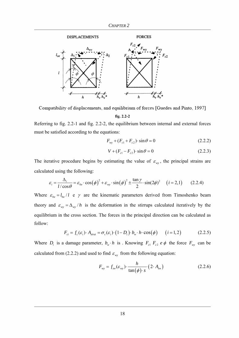
shear components are obtained independently by a truss model (fig. 2.2-1).
fig. 2.2-1
The truss consists in two concrete struts whose slope represents the direction of principal
stresses and strains, and longitudinal and transverse steel beam. The equilibrium and
compatibility are shown in fig. 2.2-2
CHAPTER 2
18
fig. 2.2-2
Referring to fig. 2.2-1 and fig. 2.2-2, the equilibrium between internal and external forces
must be satisfied according to the equations:
1 2( ) sin 0wy c cF F F θ+ + ⋅ = (2.2.2)
1 2( ) sin 0c cV F F θ+ − ⋅ = (2.2.3)
The iterative procedure begins by estimating the value of wyε , the principal strains are
calculated using the following:
( ) ( ) ( )2 2 20
tancos sin sin(2 ) 2,1/ cos 2
ii e wy i
lγε ε φ ε φ φ
θΔ
= = ⋅ + ⋅ ± ⋅ = (2.2.4)
Where 0 0 /e el lε = e γ are the kinematic parameters derived from Timoshenko beam
theory and /wy wy hε = Δ is the deformation in the stirrups calculated iteratively by the
equilibrium in the cross section. The forces in the principal direction can be calculated as
follow:
( ) ( ) ( )( ) ( ) 1 1, 2cosci c i strut c i i wF f A D b h iε σ ε φ= ⋅ = ⋅ − ⋅ ⋅ =⋅ (2.2.5)
Where iD is a damage parameter, wb h⋅ is . Knowing 1 2c cF F e φ the force wyF can be
calculated from (2.2.2) and used to find wyε from the following equation:
( ) ( )( ) 2
tanwy sw wy swhF f A
sε
φ= ⋅ ⋅ ⋅
⋅ (2.2.6)

Fibre beam-column element with flexure-shear interaction: state of the art
19
If the two subsequent values of wyε match with a predetermined tolerance, the solution is
found, otherwise the iterative procedure continue. At the end of each iteration shear
resisting forces V are estimated for each cross section.
The stiffness matrix, which the authors suggest to use, is derived from classic Timoshenko
beam element keeping uncoupled flexure and shear. the following consideration can be
made:
• The nonlinear behavior is derived from the use of the uniaxial constitutive
relationship σ ε− , the tangent modulus is obtained step-by-step. The costitutive
relationship used by the author is shown in fig. 2.2-3
• A simple liner elastic relationship can be used to represent the relation between the
shear forces V and the shear deformation γ in the truss model.
fig. 2.2-3
This was one of the first attempts to model the shear behavior in a fiber element.
The model presented is a 3D beam-column element, but the shear is modeled with a 2D
mechanism. Furthermore, the truss model is not able to take into account other shear
resistance mechanisms such as dowel action, arch action, aggregate interlock, compressive
concrete that contribute to increase the beam-column shear capacity.
Questo fu uno dei primi tentativi nel quale si cercò di modellare il comportamento a taglio
in un elemento a fibre.
Another limitation is represented by the inclination of the cracks that is fixed, equal to 30 °
or 45 °, further the truss model is not able to catch the coupling between axial flexure and
CHAPTER 2
20
shear, in other words, the shear force has no effect on flexural response. The numerical
verification highlight that the model did not represent the crack-closing phenomenon, so
the pinching effect is amplified.
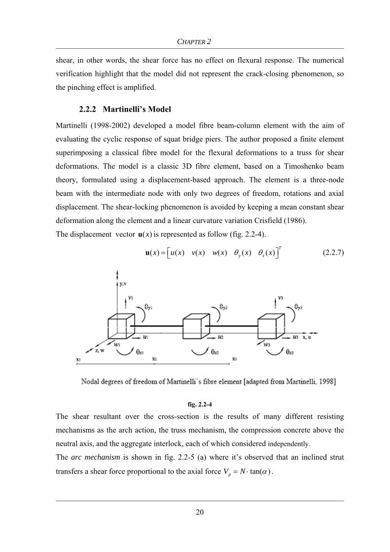
2.2.2 Martinelli’s Model
Martinelli (1998-2002) developed a model fibre beam-column element with the aim of
evaluating the cyclic response of squat bridge piers. The author proposed a finite element
superimposing a classical fibre model for the flexural deformations to a truss for shear
deformations. The model is a classic 3D fibre element, based on a Timoshenko beam
theory, formulated using a displacement-based approach. The element is a three-node
beam with the intermediate node with only two degrees of freedom, rotations and axial
displacement. The shear-locking phenomenon is avoided by keeping a mean constant shear
deformation along the element and a linear curvature variation Crisfield (1986).
The displacement vector ( )xu is represented as follow (fig. 2.2-4).
( ) ( ) ( ) ( ) ( ) ( )T
y zx u x v x w x x xθ θ⎡ ⎤= ⎣ ⎦u (2.2.7)
fig. 2.2-4
The shear resultant over the cross-section is the results of many different resisting
mechanisms as the arch action, the truss mechanism, the compression concrete above the
neutral axis, and the aggregate interlock, each of which considered independently.
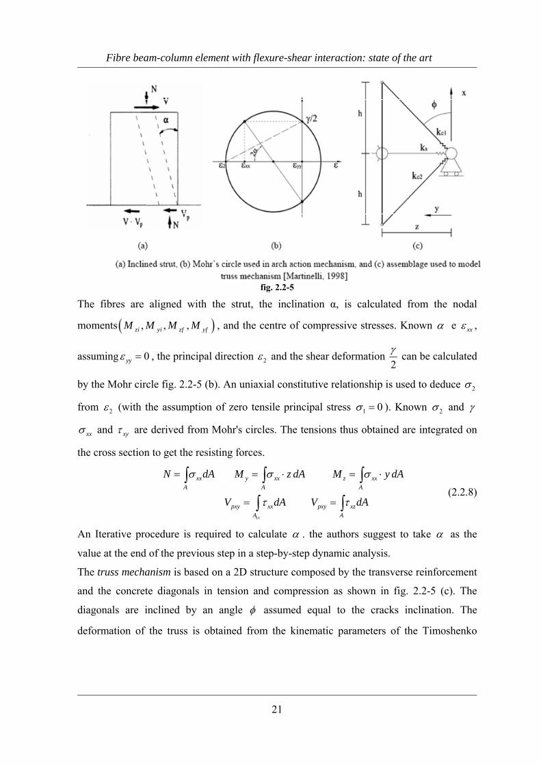
The arc mechanism is shown in fig. 2.2-5 (a) where it’s observed that an inclined strut
transfers a shear force proportional to the axial force tan( )pV N α= ⋅ .
Fibre beam-column element with flexure-shear interaction: state of the art
21
fig. 2.2-5
The fibres are aligned with the strut, the inclination α, is calculated from the nodal
moments ( ), , ,zi yi zf yfM M M M , and the centre of compressive stresses. Known α e xxε ,
assuming 0yyε = , the principal direction 2ε and the shear deformation 2γ can be calculated
by the Mohr circle fig. 2.2-5 (b). An uniaxial constitutive relationship is used to deduce 2σ
from 2ε (with the assumption of zero tensile principal stress 1 0σ = ). Known 2σ and γ
xxσ and xyτ are derived from Mohr's circles. The tensions thus obtained are integrated on
the cross section to get the resisting forces.
cc
xx y xx z xxA A A
pxy xx pxy xzA A
N dA M z dA M y dA
V dA V dA
σ σ σ
τ τ
= = ⋅ = ⋅
= =
∫ ∫ ∫
∫ ∫ (2.2.8)
An Iterative procedure is required to calculate α . the authors suggest to take α as the
value at the end of the previous step in a step-by-step dynamic analysis.
The truss mechanism is based on a 2D structure composed by the transverse reinforcement
and the concrete diagonals in tension and compression as shown in fig. 2.2-5 (c). The
diagonals are inclined by an angle φ assumed equal to the cracks inclination. The
deformation of the truss is obtained from the kinematic parameters of the Timoshenko
CHAPTER 2
22
beam xxε and xyγ where yyε it is assumed equal to the strain in the stirrups and is calculated
by imposing the equilibrium of the truss along y 0yyσ = .
Using the Mohr circles of the principal directions are simply calculated, and xyτ can be
deduced by knowing the principal stresses. The shear transferred by the truss is calculated
by integrating the shear stress over the tensioned concrete in the cross section t xy tV Aτ= ⋅ .
concrete tangent modulus 1E and 2E in principal direction and steel tangent modulus
sE can be also evaluated. By the tangent modulus is possible to calculate the stiffness
matrix shearK associated with the contribution of the truss.
The interlocking mechanism, is taken into account assuming a set of diagonal cracks with
constant spacing s (s a model parameter), inclined by an angle φ kept constant, respect to
the beam axis. The shear component xyINτ on the cross section are derived from the stresses
arising at crack faces, due to the relative displacement. These stresses are calculated from
the strains xxε , xyγ e yy sε ε= derived from the truss mechanism. The shear force
associated to the interlocking mechanism is derived from the integration of the shear
stresses xyINτ over the tensioned concrete area: IN xyIN tV Aτ= ⋅
The shear resistance force is given by the sum of the contribution of pV , tV e INV and the
stiffness matrix of the section is the following:
2
2
0 0
0 0
0 0
0 0 0 00 0 0 0
A A A
A A A
s
A A A
shear
shear
EdA y EdA z EdA
y EdA y EdA y z EdA
z EdA y z EdA z EdA
⎡ ⎤− ⋅ ⋅⎢ ⎥⎢ ⎥− ⋅ ⋅ − ⋅ ⋅⎢ ⎥⎢ ⎥
= ⎢ ⎥⋅ − ⋅ ⋅ − ⋅⎢ ⎥⎢ ⎥⎢ ⎥⎢ ⎥⎣ ⎦
∫ ∫ ∫
∫ ∫ ∫
∫ ∫ ∫K
KK
(2.2.9)
where E is the elastic tangent modulus and shearK is obtained by the truss mechanism.
A positive characteristic of this model is that it takes into account different shear resisting
mechanisms. In particular, the arch effect and the flexural behavior are formulated in 3D,
while other mechanisms are studied separately in planes xy and xz.

Fibre beam-column element with flexure-shear interaction: state of the art
23
This means that the actual spatial behavior of the model is sometimes lost. It is also noted
that in the arch effect the contribution of the shear depends on α and xxε , that are flexure-
dependent parameter, so flexure and shear in the truss mechanism are actually coupled.
In the truss mechanism the inclination of the cracks and the crack spacing are assumed
constant, thus the effect of the longitudinal reinforcement is no taken into acount.
The deformation involved are xyγ and yyε (neglected in the arch mechanism) are calculated
iteratively until the equilibrium in y direction is reached.
The solution of the aggregate interlock is derived from the truss mechanism, in terms of
strains, thus the aggregate interlock is not able to influence the other mechanisms, in
particular, is not able to affect the principal stresses directions.
In the sectional stiffness matrix the shear contribution is given only by the truss mechanism
and it is uncoupled from the flexural term. It could imply low convergence rate.
The comparisons with experimental results highlight some lacks of the model: first of all
the capability to capture some specimen collapse, furthermore it tends to exaggerate
strength degradation in cycles.
The model proposed by Martinelli [1998, 2002] is able to take into account different shear
resistance mechanisms studied independently. While failing to capture a full coupling
between axial, flexure and shear forces, it still can capture the behaviour of reinforced
concrete with shear-influenced response with a very reasonable accuracy.
2.2.3 Ranzo and Petrangeli’s model
Ranzo and Petrangeli (1998) proposed a 2D fibre beam column element based on
flexibility approach, in which the bending-axial behaviour is modelled by a classical fibre
discretisation whilst the shear response is represented by a nonlinear truss model in which
is applied an hysteretic stress-strain relationship. The two different behaviours are coupled
by a damage criterion at section level and then integrated along the element.
Stress shape functions are introduced for the 2-node element (fig. 2.2-6), so that the
moment, axial and shear forces can be given by the following equations:
( ) , ( ) 1 , ( ) i ji j
M Mx xN x N M x M M V xl l l
+⎛ ⎞ ⎛ ⎞= = − − ⋅ + ⋅ =⎜ ⎟ ⎜ ⎟⎝ ⎠ ⎝ ⎠
(2.2.10)

CHAPTER 2
24
fig. 2.2-6
Three are the degrees of freedom, two rotation ,i jθ θ and an axial elongation ,δ the
displacements vector is:
[ ]( ) ( ) ( )zx u x xθ=u (2.2.11)
In terms of compatibility, curvature χ , axial deformation ε and shear strain γ of the
section are defined. Axial force and moment are functions of ( ),ε χ , while the shear force
depends on axial and shear strains ( ),ε γ .
The resulting section stiffness matrix is the following:
[ ]
1 1
2
1 1
max
0
0
( , )0 0
nfib nfib
i i i i ii i
nfib nfib
i i i i i ii i
E A E y A
E y A E y A
v γ εγ
= =
= =
⎡ ⎤⎢ ⎥⎢ ⎥⎢ ⎥
= ⎢ ⎥⎢ ⎥⎢ ⎥∂⎢ ⎥
∂⎢ ⎥⎣ ⎦
∑ ∑
∑ ∑sk (2.2.12)
the stiffness matrix highlights the lack of coupling between shear and bending at the
section level.

Fibre beam-column element with flexure-shear interaction: state of the art
25
fig. 2.2-7
In fig. 2.2-7 can be observed the schematization of the model, concrete is represented as a
single truss element whose area is a percentage of the total section. This percentage depend
on the neutral axis at the flexure cracking point. The shear reinforcement, is equivalent to a
chord whose area is equal to the sum of shear reinforcement plus a percentage of the
longitudinal bars. Solving the strut-and-tie model, the V γ− curve is found, having
assumed a constant value for the inclination of the cracks φ. V γ− curve is defined as a
function of the applied load N, shear reinforcement and diagonal concrete struts. This
curve is obtained by applying small increments ( )iVΔ until the failure is reached, with the
distortion ( )
u uz v z
γ ∂ ∂= ≅
+ ∂. To obtain a continue curve, an analytical function is used to
interpolate these points. This procedure leads to the determination of the cracking, yielding
and ultimate shear force and distortion.
To relate the shear strength to the ductility, there are many branches of the hysteretic
relationship V γ− incorporates a degradation criterion, the primary curve is function of the
axial strain, chosen as damage indicator
(

CHAPTER 2
26
fig. 2.2-8).
Like other models based on a truss mechanism, the shear strength is the resultant of
different mechanisms (ductility-dependent concrete contribution and truss mechanism
formed by the transverse reinforcement).
fig. 2.2-8
In this model flexural and shear behaviour works in series without any specific coupling
between axial, flexure and shear components, this characteristic is underlined in the
stiffness matrix components.
Some of the assumptions are based on empirical considerations that are not necessarily
theoretically-based nor experimentally-validated. First of all the location of the equivalent
struts is given by the assumption that the axial force N is parallel to the transversal steel, in
this way the proposed system configuration is able to reproduce the correct damage

Fibre beam-column element with flexure-shear interaction: state of the art
27
sequence. Further, the cracking angle φ is assumed constant, with an average value (30° or
45°), whilst the contribution of the longitudinal bars in the truss mechanism is simply
estimated by the author.
The primary V γ− skeleton curve of the hysteretic shear relationship has been calibrated
using a nonlinear truss model, whilst a simplified damage criterion has been used to take
into account the degradation of the curve due to flexure-shear interaction]. A calibration
procedure is required for each analysis and for each structural element to be studied. This
mean that this model is very limited in general applications.
2.3 Fibre Beam-Column Element Using Microplane Model
The Microplane model family Bazant and Oh (1985), Bazant and Prat (1988) Bazant and
Ozbolt (1990), Ozbolt and Bazant (1992) is based on a kinematic constraint that links the
external deformation with slected internal planes, and the simple monitoring of the stress -
strain relations on these planes. The state of each Microplane is characterized by axial and
shear strains which makes it possible to match any Poisson ratio value.
This approach allows to describe a multi-axis response through a combination of uniaxial
constitutive laws.
2.3.1 Petrangeli’s Model
Petrangeli et al. (1996.1999) developed a fiber element based on flexibility approach to
model the shear behavior and its interaction with the bending moment and axial force in
reinforced concrete columns. The element is a 2D beam with two nodes and three degrees
of freedom per node:
[ ]( ) ( ) ( ) ( )zx u x v x xθ=u (2.3.1)
Tension and deformation vectors are the following:
( ) [ ] ( ) [ ]0 , , ,N M Vξ ε χ γ ξ= =q p (2.3.2)
Where ξ is the normalized abscissa, the beam forces p are related to the nodal
forces , ,j j iN M M , and plane sections remain plane in order to determine the longitudinal
strain xxε . To evaluate the transverse strains are assumed several shape functions Vecchio
Collins (1988). In addition to the classical assumption derived by the Timoshenko beam
theory, that keep the shear strain constant along the depth of the section, the authors have

CHAPTER 2
28
also introduced a parabolic distribution obtaining equally acceptable results in both cases.
To determine the deformations in the transverse direction yyε , the equilibrium in y
direction between concrete and steel is imposed in this way an itterative procedure begin in
order to determine a complete deformation vector xx yy xyε ε ε⎡ ⎤⎣ ⎦ associated with each
layer. Once known the deformation vector a biaxial constitutive law is applied in order to
determine the tension vector. For each fibre an incremental constitutive relationship is
derived from the static condensation of the degrees of freedom in y direction.
i ii ixx xxa asi ii ixy xysa s
d dK Kd dK Kσ εσ ε
⎡ ⎤ ⎡ ⎤⎡ ⎤= =⎢ ⎥ ⎢ ⎥⎢ ⎥
⎢ ⎥ ⎢ ⎥⎣ ⎦⎣ ⎦ ⎣ ⎦ (2.3.3)
The stiffness coefficient are calculated as follow:
( ) ( )( ) ( )
11 21 12 33 23 32
13 23 12 31 32 21
,
,
i i i i i i i i i ia s
i i i i i i i i i ias sa
K D D D K D D D
K D D D K D D D
α α
α α
= − ⋅ ⋅ = − ⋅ ⋅
= − ⋅ ⋅ = − ⋅ ⋅ (2.3.4)
iα is a percentage of the transverse reinforcement and imnD are the coefficient of the
material matrix in the i-th fibre .
As constitutive relationship for concrete, the authors chose a modified microplane model "
which links together and an equivalent uniaxial rotating model. In particular, in the
modified model, only microplane normal components are monitored. Strains are
subdivided into “weak” and “strong” components along the principal strain directions,
therefore, tensions are found for the two directions w (weak) s (strong)
( );w w s s wk k k k ks s e s C e= = ⋅ (2.3.5)
For each k-th micoplane. Regardind weak microplane, the costitutive model is based on
Mander et. al (1988), while for the stroger one, a linear elastic relationship is used. Stresses
and strains are calculated as follow:
;w s w sk k k k k ke e s sε σ= + = + (2.3.6)
Tension vector xx yy xyσ σ τ⎡ ⎤= ⎣ ⎦σ is derived by the virtual work principle, while the
material matrix D can be obtained using an incremental form of constitutive relationship.
Both σ and D are numerically evaluated, by monitoring a suitable number of microplanes.
(generally eight).
Stress-strain relationship for steel is described by Menegotto and Pinto (1977).

Fibre beam-column element with flexure-shear interaction: state of the art
29
The originality of this model compared to the strut and tie is the introduction of a biaxial
constitutive law based on a "Microplane. The biaxial approach of this formulation lead
toward an advanced model, able to describe in a more accurate manner the behaviour of
reinforced concrete structure without superimposition of different models.
On the other hand is difficult to get the influence of the different contributions to the shear
resistance. Indeed, the author reports deficiencies in the introduction of the dowel effects
as well as the relative displacement of the concrete surfaces across large cracks.
Further this model tend to underestimate the shear resistance in some areas of the beam
where the shear resistant mechanism is well represented with a strut and tie, since the local
effects caused by support and loading details cannot be predicted with the proposed
formulation, according to the author. The computational complexity of the model is similar
to the others analyzed so far while no deterrent effect are taken into account in this
element. Particularly considering that the macro stress tensor σ and the concrete fibre
constitutive matrix D must be numerically evaluated for each fibre and for each load step.
2.4 Fibre Beam-Column Element Using Smeared Crack Models
In this approach, the cracked concrete is modeled as an orthotropic material, continuous, in
which compatibility, equilibrium and constitutive relationship are formulated in terms of
average stresses and strains. This approach is particularly suitable for the analysis of a
single section under combined loads as shown in the following paragraph.
2.4.1 Vecchio and Collins’s model
Vecchio e Collins (1988) introduced the "dual-section analysis" to predict the response of a
reinforced concrete beam subject to shear, the authors developed a sectional model only,
without introducing it within a finite element.
The beam is a 2D plane and the section is discretized by layers as shown in fig. 2.4-1, the
only compatibility relationship required is the plane section remain plane after
deformation, The shear stresses calculation is carried out by finite differences between
normal stresses evaluated at each end of the fibre.

CHAPTER 2
30
fig. 2.4-1
2 1( ) ( )1( ) ( )( )
b
yxx xx xx xx
xyy
x xx b y dy doveb y x x S
σ σ σ στ−
∂ ∂ −= − ⋅ ⋅ ≈
∂ ∂∫ (2.4.1)
by is the coordinate of the last fibre, 2 1( ) ( )xx xxx e xσ σ are the normal tension in
fibres evaluated in two section separated by a distance S (this distance is assumed d/6
with d = beam depth).
The iterative procedure for the analysis of the section is represented in the follow flow
chart fig. 2.4-2.

Fibre beam-column element with flexure-shear interaction: state of the art
31
fig. 2.4-2
The analysis starts with the estimation of shear and axial strains. The equilibrium for each
one of the two sections at distance S is satisfied by an inner loop. Outer loop checks if the
shear stress calculated are equal (within an acceptable tolerance) to the initially assumed
one. Vecchio and Collins (1988) proposed two alternative and approximate solutions based
on a constant or a parabolic shear strain with the aim of simplifying the procedure. This
improvement eliminate the iterations on shear strains estimates (indicated with an asterisk
in the flowchart of fig. 2.4-2.). Generally the approximate procedures is close to more
accurate full dual-section analysis approach in terms of global behaviour.
The constitutive relationship adopted was the modified compression field theory (MCFT),
which in its first formulation (Vecchio Collins (1986)) was able to reproduce only
monotonic loadings. In twenty years, some improvement of the theory where carried out in
order to pass these limitation.

CHAPTER 2
32
According to MCFT theory, the cracked concrete is considered as an orthotropic material
along the two principal stress and strain direction as shown in fig. 2.4-3.
fig. 2.4-3
Vecchio and Collins’s sectional model use an iterative procedure in order to calculate the
shear distribution over the section. This approach give accurate results for beam subjected
to monotonic loading while the procedure is really time-consuming if implemented in a
finite element program. The dual-section analysis features also inherent difficulties in
accurately evaluating the shear stress profile on the two sections in a numerical stable
manner Benz (2000).
Indeed, the two sections must be evaluated to the same value of shear and axial load, in
order to avoid numerical instabilities. Even a small difference in axial force between the
two sections implies inaccuracy in shear stress profile. Discontinuities in shear stress
profile could be predicted for different depths of cracking subjected to different moments.
This problem, was overcame by Vecchio and Collins [1988] using a kinematics constraint,
or rather the introduction of a shear strain or shear stress distribution, in the definition of the
shear profile. This makes the procedure more stable and simple, and even if in this way the
shear stress cannot satisfy section equilibrium (because of open shear stress profile), the
approximation is considered by the author consistent with the approximation of the model.
The model can predict shear strength very well compared with the experimental results, an
exception are those beams lightly shear reinforced. This limitation (reduced accuracy in
shear-critical beams containing very little or no transverse reinforcement), Vecchio (2000)
introduced a new conceptual model for describing the behaviour of cracked reinforced
concrete − the Disturbed Stress Field Model DSFM.

Fibre beam-column element with flexure-shear interaction: state of the art
33
Finally, since the analytical procedure is a sectional model based on the assumption that
plane sections remain plane, it is not capable of predicting the local effects present in the
loading and support zones.
2.4.2 Bentz’s Model
To overcome the limitations of the dual section analysis, Benz (2000) proposed an
approach called Longitudinal sectional stiffness method. This approach was formulated for
predicting the load-deformation response of RC sections subjected to bending moments,
axial loads and shear forces. The assumption of this procedure are plane sections remain
plane and the distribution of shear stresses across the section is defined by the rate of
change of flexural stresses. An initial shear strain profile is required as function of the
mean sectional shear deformation γ (for the first load step, the elastic Jourawski solution
is assumed):
( )( )xy
A Q y VconI b y A
γ γ γ⋅= ⋅ =
⋅ (2.4.2)
Once calculated the axial deformation of the beam with the classic Eulero Bernoulli theory
and shear deformation with (2.4.2), the relationship between the section’s elongation,
curvature and mean shear strain and the fibre strains can be derived :
ˆ( ) sx = ⋅ε B ε (2.4.3)
Where ˆ( ) xx xyx ε γ⎡ ⎤= ⎣ ⎦ε e [ ]0s ε χ γ=ε .
At each fibre, the differential increment of stress along the beam axis can be computed as
follows
ntd dε= ⋅σ D (2.4.4)
In which ntD is the nodal tangent stiffness matrix, xx yy xyε ε γ⎡ ⎤= ⎣ ⎦ε and
xx yy xyσ σ τ⎡ ⎤= ⎣ ⎦σ .
For the equilibrium in the transverse direction, the component 0yyσ = at each fibre.
Fron this equilibrium equation a static condensation of the DOF in the y-direction is
obtained, and an incremental constitutive relation is derived:
ˆ ˆˆ ˆxx xxnt nt
xy xy
d dd d
d dσ ετ γ
⎡ ⎤ ⎡ ⎤= = ⋅ = ⋅⎢ ⎥ ⎢ ⎥⎣ ⎦ ⎣ ⎦
σ D D ε (2.4.5)
CHAPTER 2
34
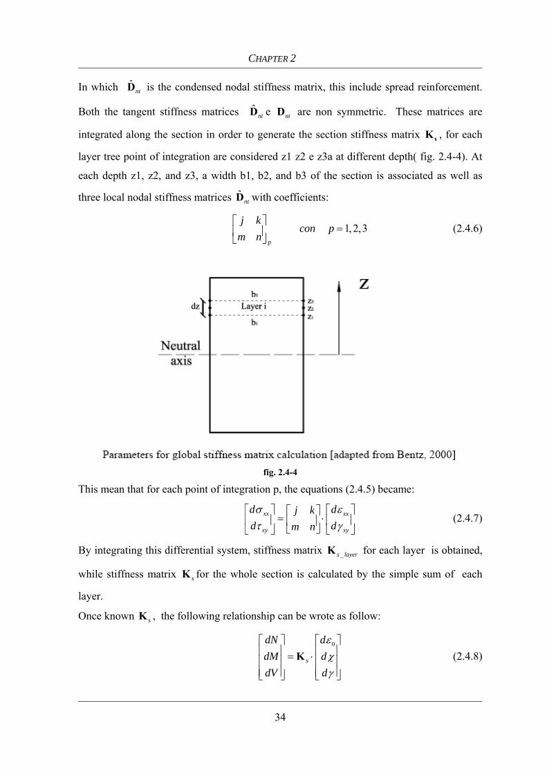
In which ˆntD is the condensed nodal stiffness matrix, this include spread reinforcement.
Both the tangent stiffness matrices ˆntD e ntD are non symmetric. These matrices are
integrated along the section in order to generate the section stiffness matrix sK , for each
layer tree point of integration are considered z1 z2 e z3a at different depth( fig. 2.4-4). At
each depth z1, z2, and z3, a width b1, b2, and b3 of the section is associated as well as
three local nodal stiffness matrices ˆntD with coefficients:
1, 2,3p
j kcon p
m n⎡ ⎤
=⎢ ⎥⎣ ⎦
(2.4.6)
fig. 2.4-4
This mean that for each point of integration p, the equations (2.4.5) became:
xx xx
xy xy
d dj kd dm nσ ετ γ
⎡ ⎤ ⎡ ⎤⎡ ⎤= ⋅⎢ ⎥ ⎢ ⎥⎢ ⎥⎣ ⎦⎣ ⎦ ⎣ ⎦
(2.4.7)
By integrating this differential system, stiffness matrix _s layerK for each layer is obtained,
while stiffness matrix sK for the whole section is calculated by the simple sum of each
layer.
Once known sK , the following relationship can be wrote as follow:
0
s
dN ddM ddV d
εχγ
⎡ ⎤ ⎡ ⎤⎢ ⎥ ⎢ ⎥= ⋅⎢ ⎥ ⎢ ⎥⎢ ⎥ ⎢ ⎥⎣ ⎦ ⎣ ⎦
K (2.4.8)

Fibre beam-column element with flexure-shear interaction: state of the art
35
Sinche the deformation incrementi s given by the following equation:
1
0
0
ss
dNdx
d dM vdx dx
dVdx
−
⎡ ⎤=⎢ ⎥⎢ ⎥⎢ ⎥= ⋅ =⎢ ⎥⎢ ⎥⎢ ⎥=⎢ ⎥⎣ ⎦
ε K (2.4.9)
Using the (2.4.5), (2.4.3) and the (2.4.9) and changing the variable the following
relationship can be reached:
1
0ˆ ˆ ˆ ˆ
ˆ0
s snt s
s
d dd d Vdx d d dx
−
⎡ ⎤⎢ ⎥= = ⋅ ⋅ ⋅ ⎢ ⎥⎢ ⎥⎣ ⎦
σ εσ ε D B Kε ε
(2.4.10)
In the end, the xyτ diagram can be calculated by introducing xxddxσ evaluated by (2.4.10) in
(2.4.1) equation.
The constitutive relationship used by Benz is MCFT, this formulation can satisfy the
equilibrium between the fibre and is able to calculate the resistance and the deformation in
a section subjected by M, N, and T. The Hypothesis of plane section remain plane and
0yyσ = limit the range of validity of the analysis away from the restrained areas and
concentrated loads, the response of elements without shear reinforcement tends to be
inaccurate because of the limitations inherent in MCFT. The cyclical behavior of the
material has not been implemented, the model also has not been tested in a finite element
program which could assemble complex structures.
2.4.3 Remino’ Model.
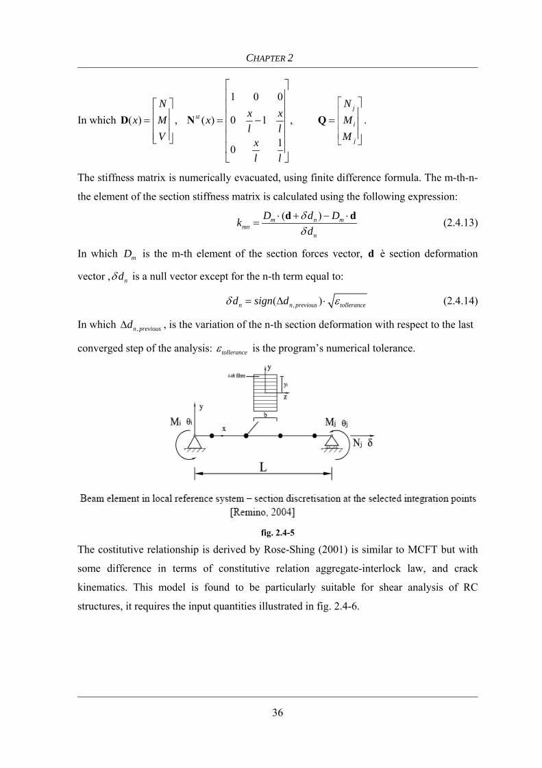
Remino (2004) formulated a fibre Timoshenko force-based beam-column element. The
force-based formulation is based on the solution strategy proposed by Spacone et al.
(1996). The element (shown in fig. 2.4-5 with without rigid body movements) has two
nodes and two degrees of freedom per node:
[ ]( ) ( ) ( )zx u x xθ=u (2.4.11)
From the nodal forces Q , the section force vector ( )xD is computed as follows:
( ) ( )stx x= ⋅D N Q (2.4.12)
CHAPTER 2
36
In which
1 0 0
( ) , ( ) 0 1 ,
10
jst
i
j
N Nx xx M x Ml l
V Mxl l
⎡ ⎤⎢ ⎥
⎡ ⎤⎡ ⎤ ⎢ ⎥⎢ ⎥⎢ ⎥ ⎢ ⎥= = − = ⎢ ⎥⎢ ⎥ ⎢ ⎥⎢ ⎥⎢ ⎥ ⎢ ⎥⎣ ⎦ ⎣ ⎦
⎢ ⎥⎣ ⎦
D N Q .
The stiffness matrix is numerically evacuated, using finite difference formula. The m-th-n-
the element of the section stiffness matrix is calculated using the following expression:
( )m n mmn
n
D d Dkd
δδ
⋅ + − ⋅=
d d (2.4.13)
In which mD is the m-th element of the section forces vector, d è section deformation
vector , ndδ is a null vector except for the n-th term equal to:
,( )n n previous tolleranced sign dδ ε= Δ ⋅ (2.4.14)
In which ,n previousdΔ , is the variation of the n-th section deformation with respect to the last
converged step of the analysis: tolleranceε is the program’s numerical tolerance.
fig. 2.4-5
The costitutive relationship is derived by Rose-Shing (2001) is similar to MCFT but with
some difference in terms of constitutive relation aggregate-interlock law, and crack
kinematics. This model is found to be particularly suitable for shear analysis of RC
structures, it requires the input quantities illustrated in fig. 2.4-6.

Fibre beam-column element with flexure-shear interaction: state of the art
37
fig. 2.4-6
The main characteristic of this model is the implementation of a "smeared crack" in a
program fem for the analysis of complete structures. A direct interaction between the
section forces is considered. Unfortunately, numerical difficulties were found in analyzing
the cyclical behavior of the fibers, the numerical results compared with the experimental
data are not always accurate.
2.4.4 Bairan’s Model
Bairan (2005) developed a 3D model for the analysis of reinforced concrete sections
subject to bending moment, shear, axial force and torque. The author designed a model that
considers the section distortion due to shear and torque through a generalized state of
stress strain of the section. This approach allows consider the equilibrium of the section
separated from the equilibrium of whole beam, allowing the introduction of models
developed separately for sections, in any type of beam formulation.
Given a section, the whole 3D state is obtained through the distorting effects wu superimposed to the traditional ones due to the conservation of plane sections psu , the
physical meaning of this decomposition is schematically shown in fig. 2.4-7.

CHAPTER 2
38
fig. 2.4-7
While the structural equilibrium is insured by the resisting forces derived from psu , the
sectional equilibrium is given by the internal forces resulting from wu . Since the
displacement field is decomposed as follows:
ps w= +u u u (2.4.15)
The same decomposition can be applied in stress and strain field as follow:
ps w ps we= + = +ε ε ε σ σ σ (2.4.16)
Rewriting in the weak form the 3D differential equilibrium equations of an elementary
volume using as weighting function the displacement field u, the following residual
equations of a beam differential element are obtained:
( ) ( ) ( )( ) ( ) ( )
( ) ' 0
( ) ' 0
ps ps ps ps ps w
w w w ps w w
x
x
⎧ = − − =⎪⎨
= − − =⎪⎩
R G σ F σ F σ
R G σ F σ F σ (2.4.17)
In which ( )ps xR is the residual in the space of the plane-section displacement field, and
( )w xR is the residual in the space of the distortion displacement field. This approach
consists in founding an appropriate expression of wσ to satisfy the equation ( ) 0w x =R ,
which represents the cross-section constitutive relation, and then in solving the beam
equilibrium equation ( ) 0ps x =R . So the procedure aims to solve a 3D problem through
two decoupled components: a 1D beam problem, using standard frame elements to

Fibre beam-column element with flexure-shear interaction: state of the art
39
discretise the plane section field and a 2D sectional problem, using bi-dimensional
elements, locally at the beam’s integration points, to discretise the distortion field
(equations (2.4.17)). In particular, in the case of RC beams, the sections are subdivided in
2D elements simulating the concrete matrix, 1D elements simulating the transversal
reinforcements, and point elements simulating the longitudinal reinforcements. Indicated
with wd the vector of nodal values of these elements, the distortion field results:
w w w= ⋅u N d (2.4.18)
with wN interpolation matrix that contain shape functions. Imposing that the nodal
distorsion satisfy the equilibrium over the control sections:
* *w = ⋅d A ξ (2.4.19)
In which * * *' ' ' ' '0 0s s x y z x y zε χ χ χ ε χ χ χ⎡ ⎤ ⎡ ⎤= =⎣ ⎦ ⎣ ⎦ξ e e is the generalized
deformation vector of the section and its derivative, the matrix *A is derived by the
material stiffness matrix D , the shape functions wN are the derivate of wB and *psB which
are the fuctions that interpolate the deformations *se . Referring to (2.4.16) the strains can
be expressed as:
* *ps ps w w w ws e= ⋅ = ⋅ = ⋅ ⋅ε B e ε B d B A ξ (2.4.20)
where 0s xy xz x y zε χ χ χ χ χ⎡ ⎤= ⎣ ⎦e is the vector of generalised section strains, and
the matrix psB is the strain interpolation matrix for se .
From (2.4.20), it can be noticed that the distortion field is a linear function of the eight
components of the vector ξ* , in which two components are not independent from the
others. Hence, a reduction of the required degrees of freedom (from 8 to 6) is obtained by
means of the matrix Ξ which condensates the derivatives of axial elongation and torsion
curvature taking into account the actual distributed axial load and torsion moment.
* = Ξ ⋅ξ ξ (2.4.21)
A crucial step of the model is expressing the ξ vector as a function of the generalized
section strains. To reach this goal, the author introduces the generalized shear deformation
through the virtual work principle, reaching the following relationship:
s= ⋅ξ Ω e (2.4.22)
noting that such matrix Ω has not been explicitly defined for the case of a generic RC

CHAPTER 2
40
section. Substituting the (2.4.22) and (2.4.21) in (2.4.19) the distortion nodal values
result:
*ws= ⋅ ⋅d A Ω e (2.4.23)
implying that the non-local contribution due to the distortion-warping field can be
computed as a function of local variables alone, in particular the generalised section
strains. A new definition of wε is obtained by substituting the (2.4.23) in (2.4.20) , whilst
the stresses of Eq. (2.4.16) can be derived from the following equations:
ps ps w we= ⋅ = ⋅σ D ε σ D ε (2.4.24)
In which D is the material matrix, which can be of any type, in general anisotropic.
Finally, through the virtual work principle, the generalized stresses ss are derived and
hence the section stiffness matrix is obtained:
*
*
* * *
psT T T T psTs
A A
psT ps psT ws
A A
T T T wT w T T T wT w
A A
dA dA
dA dA
dA dA
= +
= ⋅ ⋅ + ⋅ ⋅ ⋅ ⋅ ⋅ +
+ ⋅ ⋅ ⋅ ⋅ ⋅ + ⋅ ⋅ ⋅ ⋅ ⋅ ⋅ ⋅ ⋅
∫ ∫
∫ ∫
∫ ∫
s B σ Ω Ξ A B σ
K B D B B D B A Ω Ξ
Ω Ξ A B D B Ω Ξ A B D B A Ω Ξ
(2.4.25)
For the constitutive model was implemented a rotating smeared crack, in which the
material behavior is described along the principle directions. For concrete in compression
is considered Vecchio Selby (1991) relationship able to model the cyclic loading. For the
concrete in tension is considered a linear elastic behavior until the cracking and a
descending curve after cracking described by Cervenka (1985), unloading and reloading
are assumed linear. For steel has taken a classic elastic-plastic model.
The author used a triaxial stress state to calculate the resistance in the principle directions
of breaking through a domain consists of a three-dimensional surface. The stiffness matrix
of the material is calculated along the principal directions, then rotated in the x-y direction
through an appropriate transformation matrix. Before transformation the matrix result
diagonal, whose elements are the secant modulus of the principal directions. The shear
modulus is given by
( )( )
12
i jij
i j
Gσ σ
ε ε
−=
− (2.4.26)

Fibre beam-column element with flexure-shear interaction: state of the art
41
To summarize: the model proposed by Bairan is able to simulate the complete interaction
between the six components of internal action and deformation of a general cross section
with an arbitrary arrangement of longitudinal reinforcement. This element is certainly an
advanced model for reinforced concrete elements, obtained developing a sectional model
in which the non-local effects due to section’s warping-distortion induced by shear/torsion
are derived from local quantities such as the generalized section strains. Hence,
equilibrium and compatibility at the sectional level (inter-fibre equilibrium) are satisfied
because no a priori hypotheses on the shear flow or strain distribution are needed.
On the other hand the development of the model also requires some approximations with
regard to the distortion field and its the discretization, the variation of distortion along the
beam, the behaviour of the material and the discretization of the section. It’s not clear how
these might affect the quality of approximations, the numerical stability and the field of
applicability of the method. Future developments include the implementation of the
sectional model proposed in a finite element program for analysis of frames subject to
static and dynamic loads. Through this route is expected to give an answer to previous
questions.
2.5 Fibre Beam-Column Element Using Damage Models.
The damage models require some concepts of fracture mechanics to simulate the
propagation of cracks. These include parameters such as fracture energy, which represents
the energy required to create a new rupture of the material expressed unit per length. This
parameter is an intrinsic characteristic of the material for concrete and its value is about
0,3fkNmG
m= .
2.5.1 Modello di Mazars
Mazars et al. (2006) developed a 3D element with stiffness approach based on
Timoshenko beam theory. The interpolation functions depends on the material properties
(Young's modulus and shear modulus for each fiber) only in the first step of loading, while
in the following functions are assumed constant. The finite element with two nodes and six
degrees of freedom per node, is shown in fig. 2.5-1 while the displacement vector is the
following:

CHAPTER 2
42
( ) ( ) ( ) ( ) ( ) ( ) ( )x y zx u x v x w x x x xθ θ θ⎡ ⎤= ⎣ ⎦u (2.4.27)
The section stiffness matrix Ks, relating the vectors of the generalized
stresses x y x y zN V V M M M⎡ ⎤⎣ ⎦ and strains (with rigid body movements eliminate)
is the calculate as follow:
( )2 2
2
2
0 0 0
0 0 0 0
0 0 0 0
0 0 0 0 0
0 0 0 0
0 0 0 0 0
A A A
y yA A
zA A
s
z z yA
A A
A
E dA E z dA E y dA
k G dA k G z dA
G dA k G y dA
k G k y k z dA
E z dA E y z dA
E y dA
⎡ ⎤⋅ − ⋅⎢ ⎥⎢ ⎥
⋅ − ⋅ ⋅⎢ ⎥⎢ ⎥⎢ ⎥⋅ ⋅⎢ ⎥⎢ ⎥=⎢ ⎥⋅ ⋅ ⋅ + ⋅⎢ ⎥⎢ ⎥
⋅ − ⋅ ⋅⎢ ⎥⎢ ⎥⎢ ⎥⋅⎢ ⎥⎣ ⎦
∫ ∫ ∫
∫ ∫
∫ ∫
∫
∫ ∫
∫
K (2.4.28)
Where A is the section area, E is the young modulus and G is the shear modulus, of each
fibre, y zk e k are correction factors due to shear, depending on the geometry of the section
and the material.
fig. 2.5-1
For steel a classical plasticity model is adopted while for concrete are introduce two
different damage models: Mazars (fig. 2.5-2(a)) characterized by a variable damage scale,
used for monotonic loadings and La Bordiere (fig. 2.5-2 (b)) which, having two variable
scales of damage and including the closing of cracks and permanent effects was adopted to
model cyclic loading. In any case, the damage model affects only the normal stresses.

Fibre beam-column element with flexure-shear interaction: state of the art
43
The model is affected by two main limitations, the effect of distortion and damage model
of isotropic type are not included. The latter in particular implies that the element is unable
to reproduce the typical response of anisotropic sections in reinforced concrete when the
cracks are caused by the shear. This means that the model can be used in studying the
global behavior of slender elements as shown by the numerical results for general purpose
more accurate and robust relationship are required. The use of constitutive relations with
local "strain softening"(as this case) mean that the results are mesh-dependent, thus
increasing the complexity of the model.
fig. 2.5-2

CHAPTER 3
44
Fibre beam-column beam formulation
3.1 Sommario
In questa tesi ci si propone di riuscire a modellare il comportamento di elementi strutturali in
cemento armato cercando di cogliere l’interazione che nasce tra sforzo normale, momento flettente
e taglio in campo non lineare. Per fare ciò è stato ideato un elemento finito nuovo sulla linea dei
modelli “smeared” visti nel capitolo 2. L’elemento finito in questione è un modello a fibre basato
sulla flessibilità Spacone Taucer Filippou (1996) sul quale è implementato un legame di tipo
biassiale con fessurazione diffusa, per cogliere l’accoppiamento tra le sollecitazioni e descrivere in
maniera unitaria e coerente il comportamento strutturale. In questo capitolo è descritta la
formulazione analitica dell’elemento finito a fibre, non si fa cenno al legame biassiale che sarà
trattato ampiamente nel capitolo successivo e all’implementazione completa descritta in modo
dettagliato nel capitolo 5. Verranno comunque accennati alcuni passi dell’algoritmo di Element
State Determination in quanto risulta essere una procedura fondamentale per la formulazione
completa dell’elemento.
Lo sviluppo analitico sarà svolto nella forma più generale del “mixed method” (metodo misto) visto
che questo approccio chiarisce meglio il processo di “state determination” utilizzato nell’algoritmo
di analisi non lineare.
Le ipotesi fatte alla base del sono:
• Piccole deformazioni
• Conservazione delle sezioni piane
Le sollecitazioni all’interno dell’elemento sono rappresentate attraverso una funzione
d’interpolazione che le lega alle forze nodali dell’elemento stesso, le azioni interne così ottenute
sono tali da soddisfare l’equilibrio entro l’intero elemento. Il soddisfacimento dell’equilibrio è
proprio la condizione che sta alla base del metodo.
La formulazione proposta presenta notevoli vantaggi, equilibrio e compatibilità sono ovunque
soddisfatti lungo l’elemento, l’equilibro è rispettato con la scelta delle funzioni di interpolazione, la
compatibilità è soddisfatta integrando le deformazioni delle sezioni per avere le deformazioni
dell’elemento e gli spostamenti di estremità mentre per soddisfare il legame è stata implementata
una procedura iterativa.

Fibre beam-column element formulation
________________________________________________________________________________
________________________________________________________________________________
45
3.2 Definition of the vectors involved
The finite element is schematically represented in fig. 3.2-1, in which x y are the local coordinates
while X Y represents the global reference system: in this description the following notation is
adopted: forces are represented by uppercase and displacements and deformations from the
corresponding lower case letters in bold are represented vectors and matrices.
fig. 3.2-1
1
2
3
Element nodal forcesQQQ
⎧ ⎫⎪ ⎪= ⎨ ⎬⎪ ⎪⎩ ⎭
Q (3.2.1)
1
2
3
element nodal displacementqqq
⎧ ⎫⎪ ⎪= ⎨ ⎬⎪ ⎪⎩ ⎭
q (3.2.2)
( )( )( ) section forces( )
M xx T x
N x
⎧ ⎫⎪ ⎪= ⎨ ⎬⎪ ⎪⎩ ⎭
D (3.2.3)
( )
( ) ( ) section deformation( )
xx x
x
χγε
⎧ ⎫⎪ ⎪= ⎨ ⎬⎪ ⎪⎩ ⎭
d (3.2.4)

CHAPTER 3
________________________________________________________________________________
________________________________________________________________________________
46
in order to finalize the study to the shear deformation, the extension to the spatial case was not
implemented. This extension can be obtained by adding shear and moment in and orthogonal
direction and torque. More sophisticated shape function for the section must be introduced for this
extension.
3.3 Formulation of the element starting from mixed method
In general analytical formulation of the element is not considered any constitutive relationship. In
agreement with those reported by Spacone et all.(1996) the finite element formulation is based on
the mixed method, and it is shown that the particular choice of shape functions dependent on the
flexibility, lead to a substantial simplification of the final equation. It is shown that with this
particular choice, the mixed method can be reduced to the flexibility method. However the
formalism of the mixed method is very useful for understanding the procedure of element
determination here described.
In the two fields mixed method Zienkiewicz e Taylor (1989), independent shape functions are used
to interpolate the of forces and displacements fields along the element. Called Δ the incrementi of
the corresponding quantities, the two fields can be written as follows:
( ) ( )i ix xΔ = ⋅Δd a q (3.3.1)
( ) ( ) e ( ) ( )i i i ix x x xΔ = ⋅Δ = ⋅D b Q D b Q (3.3.2)
Where ( )xa e ( )xb are respectively the interpolation matrices of deformation and forces, the
superscript i indicates the i-th iteration. Following the principle of virtual forces we can write the
following equation;
1
0
( ) ( ) ( ) ( ) 0L
T i i ix x x x dxδ δ −⎡ ⎤⋅ − ⋅Δ =⎣ ⎦∫ D d f D (3.3.3)
1( )i x−f is the flexibility matrix calculated at previous step.
Substituting (3.3.1) and (3.3.2) in (3.3.3) the following equation can be written:
1
0
( ) ( ) ( ) ( ) 0L
T T i i ix x x x dxδ −⎡ ⎤⋅ ⋅ ⋅Δ − ⋅ ⋅Δ =⎣ ⎦∫Q b a q f b Q (3.3.4)
Since equation (3.3.4) must hold for any TδQ , it follows that:
1
0 0
( ) ( ) ( ) ( ) ( ) 0L L
T i T i ix x dx x x x dx−⎡ ⎤ ⎡ ⎤⋅ ⋅Δ − ⋅ ⋅ ⋅Δ =⎢ ⎥ ⎢ ⎥
⎣ ⎦ ⎣ ⎦∫ ∫b a q b f b Q (3.3.5)
The expression in square brackets represent the following matrices:

Fibre beam-column element formulation
________________________________________________________________________________
________________________________________________________________________________
47
1 1
0
( ) ( ) ( )L
i T ix x x dx− −= ⋅ ⋅∫F b f b (3.3.6)
0
( ) ( )L
T x x dx= ⋅∫T b a (3.3.7)
Where 1i−F is the flexibility matrix of the element andT is a matrix that only depend on the
interpolation function matrices. Thus using (3.3.6) and the (3.3.7), the equation(3.3.5) can be
written as follow:
1 0i i i−⋅Δ − ⋅Δ =T q F Q (3.3.8)
In mixed method the integral form of equilibrium is derived from the virtual displacement principle:
1
0
( ) ( ) ( )L
T i i T ix x x dxδ δ−⎡ ⎤⋅ + Δ = ⋅⎣ ⎦∫ d D D q P (3.3.9)
where P is the vector of applied loads, in equilibrium with the internal forces; substituting the
(3.3.1) and the (3.3.2) in the (3.3.9) following equation is obtained:
1 1
0
. ( ) ( ) ( )L
T i i T ix x x dxδ δ− −⎡ ⎤⋅ ⋅ + ⋅Δ = ⋅⎣ ⎦∫q a b Q b Q q P (3.3.10)
Since equation (3.3.10) must hold for anyδq , it follows that:
1 1
0 0
( ) ( ) ( ) ( )L L
T i T i ix x dx x x dx− −⎡ ⎤ ⎡ ⎤⋅ ⋅ + ⋅ ⋅Δ =⎢ ⎥ ⎢ ⎥
⎣ ⎦ ⎣ ⎦∫ ∫a b Q a b Q P (3.3.11)
Written in matrix form:
1 1T i T i i− −⋅ + ⋅Δ =T Q T Q P (3.3.12)
Combining the equations (3.3.8) and (3.3.12) in one system of equations:
1
1
i i
i T iT i
−
−
⎡ ⎤ ⎧ ⎫− Δ ⎧ ⎫⋅ =⎨ ⎬ ⎨ ⎬⎢ ⎥ − ⋅Δ ⎩ ⎭⎣ ⎦ ⎩ ⎭
0F T QP T QT 0 q
(3.3.13)
The firs equation can be solved for iΔQ and the results substituted in the second equation. In this
way the following equation is reached:
1 1T i T i i T i− −⎡ ⎤⋅ ⋅ ⋅Δ = − ⋅⎣ ⎦T F T q P T Q (3.3.14)
The function ( ) and ( )x xa b are completely independent in the general formulation, but can be
observed in the equation (3.3.7) how with a particular choice of the shape function ( )xa , a

CHAPTER 3
________________________________________________________________________________
________________________________________________________________________________
48
remarkable simplification, in particular a function ( )xa depending on the flexibility can be chosen as
follow:
11 1( ) ( )i ix f x−− −⎡ ⎤= ⋅ ⋅ ⎣ ⎦a b F (3.3.15)
An interpolation function thus assigned relates the section deformation with the corresponding
element deformation, from (3.3.1) this equation can be written:
11 1( ) ( )i i i ix f x−− −⎡ ⎤Δ = ⋅ ⋅ ⋅Δ⎣ ⎦d b F q (3.3.16)
This particular choice of ( )xa imply that T i san Identity matrix I, recalling the (3.3.7):
11 1
0
( ) ( )L
T i ix x dx−− −⎡ ⎤
⎡ ⎤= ⋅ ⋅ ⋅ =⎢ ⎥ ⎣ ⎦⎣ ⎦∫T b f b F I (3.3.17)
With this choice of ( )xa the equation (3.3.14) is reduced to:
1 1i i i i− −⎡ ⎤ ⋅Δ = −⎣ ⎦F q P Q (3.3.18)
This choice of ( )xa reduce the mixed method to the flexibility method. The equation (3.3.18) is the
linearized realtion between applied loads 1i i−−P Q and the corrisponding deformation
increments iΔq .
Although the classical flexibility method provide the same system of equations (3.3.18), the
derivation described above has the following advantages:
• The mixed method provide directly an expression, flexiblility dependent for the deformation
shape functions ( )xa
• It show the consistent implementation of the state determination process.
• Is more general because it allow the choice of different shape functions ( )xa .
Since ( )xa and ( )xb are independent and not change during the iterative process, the proposed
method coincides with the classical flexibility method, the procedure also reduces to the stiffness
method if the constitutive relationship is linear elastic. In other words, the independence between
the two fields is not inherent in the definition of shape the functions, but comes from the material
nonlinearity.
3.4 Element state determination
The flexibility method was chosen in this work, because is shown in several studies that leads to
significant advantages in nonlinear analysis of structures. The main problem of this method is the
determination of the resisting forces starting from the deformations of the element. This problem

Fibre beam-column element formulation
________________________________________________________________________________
________________________________________________________________________________
49
arises when the finite element formulation is based on the virtual forces principle. The procedure
used in the solution of this problem is called element state determination. The problem has been
faced and solved through a procedure presented by Spacone et all. (1996).
Although the element is based on flexibility, it is implemented in a program that uses the direct
stiffness method, so every step that yield all the general displacement of the structural degrees of
freedom. Since the element is based on flexibility there aren’t shape functions that correlate
deformation strain field along the element with the nodal displacements. The process of finding the
resisting forces that correspond to the given element deformation is known as state determination.
3.4.1 Description of the procedure
The state determination process consist of three different phases:
• Section state determination: Starting from section deformation, this procedure determine the
section forces. While in general, this phase is simple and direct, in this work is represented
by a complex procedure described in next chapter.
• Element state determination: Starting from the nodal displacement, in this phase the nodal
resisting forces are calculated. Element state determination has section state determination
inside.
• Structure state determination: In this phase the forces of each element are assembled, giving
the structure resisting forces. This forces must be compared with the applied loads, this
comparison give the unbalanced forces that must be applied to the structure in an iterative
procedure until convergence is reached.
In the algorithm described below three levels of iteration are introduced, two outermost processes
denoted by k and i indices that involve structural degrees of freedom and an innermost process
denoted by index j that corresponds to the element state determination.
The section state determination is not reported in this chapeter.
In fig. 3.4-1 is represented the structure and element evolution during a load step kEΔP .

CHAPTER 3
________________________________________________________________________________
________________________________________________________________________________
50
fig. 3.4-1
3.4.2 Element state determination algorithm.
In the following pages the subsequent steps of the procedure will be described in detail, not
considering for the type of element and the section state determination in order to focus the
attention on the element state determination.
• k = denote the applied load step
• i = is the index for the Newton-Raphson iteration scheme at structural level
• j = is the index for the element state determination process.
(1) First of all the global system of equation is solved and the displacement of the structure are
updated.
1i i is E− ⋅Δ = ΔK p P (3.4.1)
1i i i−= + Δp p p (3.4.2)
(2) Deformation increment for the elements are calculated starting from nodal displacement of
the structure, subsequently the element deformation are updated.
i ieleΔ = ⋅Δq L p (3.4.3)
1i i i−= + Δq q q (3.4.4)
The matrix eleL include two transformation, tin the first the element displacement in global
reference system are transformed to the displacement in local reference system. In the second

Fibre beam-column element formulation
________________________________________________________________________________
________________________________________________________________________________
51
transformation the element displacement are transformed to the element deformation by a static
condensation that consist into an elimination of the rigid body movments.
(3) Start element state determination procedure, some iteration are carried out for each element
f the structure.
The procedure start by the calculation of the nodal forces increment in the element
1j j j−Δ = ⋅ΔQ k q (3.4.5)
When j=1 1 0j− =k k , 1 0j− =Q Q e 1j i−Δ = Δq q where i-1 correspond to the state of the element
calculated at the last Newton-Raphson iteration.
Nodal forces are updated:
1j j j−= + ΔQ Q Q (3.4.6)
(4) Determine the section forces increment for all control section.
In order to calculate the section forces the equation (3.3.2) is used; this equation relate section and
nodal forces, in the following chapters this matrix will be better explained.
( ) ( )j jx xΔ = ⋅ΔD b Q (3.4.7)
1( ) ( ) ( )j j jx x x−= + ΔD D D (3.4.8)
(5) Determine section deformation increment for each control section:
Residual deformation 1( )j x−r must be added to the previous iteration. For j=1, 0 ( ) 0x =r
1 1( ) ( ) ( ) ( )j j j jx x x x− −Δ = +⋅Δd f D r (3.4.9)
1( ) ( ) ( )j j jx x x−= + Δd d d (3.4.10)
(6) Flexibility and stiffness tangent matrix of the section 1
( ) ( )j jx x−
⎡ ⎤= ⎣ ⎦f k and the resisting
forces ( )jR xD has been subsequently calculated starting from the deformation ( )j xd .
(7) Once known the resisting forces, unbalanced section forces ( )jU xD can be calculated by the
following difference:
( ) ( ) ( )j j jU Rx x x= −D D D (3.4.11)
(8) Using the new flexibility matrix and the unbalanced forces, residual deformation can be
calculated as follow:
( ) ( ) ( )j j jUx x x= ⋅r f D (3.4.12)
(9) A new flexibility and stiffness matrix for the element can be calculated by integration:

CHAPTER 3
________________________________________________________________________________
________________________________________________________________________________
52
0
( ) ( ) ( )L
j T jx x x dx= ⋅ ⋅∫F b f b (3.4.13)
1j j −
⎡ ⎤= ⎣ ⎦K F (3.4.14)
(10) Check for the elemet convergence
If the unbalanced forces for each section are smaller than a fixed tollarence , the element have
converged and after setting i j=Q Q e i j=K K , the procedure continue. If some section have not
converged the residual element deformation sj are calculated by integration of the residual section
deformation rj(x).
0
( ) ( )L
j T jx x dx= ⋅∫s b r (3.4.15)
J is incremented as j=j+1 and the algorithm return to the step (3) with 1j j+Δ = −q s until convergence
is reached.
(11) Determine resisting forces and new stiffness matrix of the structure.
When all element have converged the i-th Newton-Raphson step is complete and the element force
vectors are assembled .
1
( )n
i T iR ele ele
ele== ⋅∑P L Q (3.4.16)
A new structure tangent stiffness matrix is than assembled as follow:
1
( )n
i T is ele ele ele
ele== ⋅ ⋅∑K L K L (3.4.17)
Where n is the number of elements of the whole structure.
The resisting forces are than compared with the applied loads and if the difference between these
forces ( iuΔP ) is greater than a fixed tolerance, the unbalanced forces imposed to the structure, the
index i is incremented in i=i+1 and the next Newton–Raphson iteration begin with 1i iu E
+Δ = ΔP P .
In this chapter there aren’t any reference to the fibers model just to focus on the formulation of the
element, in particular the flexibility method deduced from the mixed method to the description of
the element state determination. In following chapters is described the procedure applied to a fiber
element that include flexure and shear component, is also explained a section state determination
that allow the coupling of flexure and shear in nonlinear field.
CHAPTER 4
Constitutive Relationship: Section state determination
4.1 Sommario
In questo capitolo ci si propone di illustrare la teoria che sta alla base del legame
costitutivo per l’elemento finito descritto nel capitolo precedente. Come già accennato il
legame utilizzato è di tipo biassiale, le relazioni sono tratte dalla MCFT (modified
compression field theory) Vecchio Collins (1986) e sui successivi sviluppi quali la DSFM
(disturbed stress field model) Vecchio (2000). Le teorie citate sono state sviluppate per
modellare lo stato tensionale e deformativo di elementi in c.a. soggetti a stati piani di
tensione. Nel modello il c.l.s. fessurato è considerato come un materiale ortotropo in cui
equilibrio compatibilità e legame sono formulati in termini di tensioni e deformazioni
medie; a parte sono poi introdotte considerazioni sullo stato locale della fessura nella quale
sono poste delle limitazioni per quel che riguarda il livello tensionale. Tutte le relazioni per
il calcestruzzo fessurato derivano prove sperimentali su 30 provini sollecitati a diverse
sollecitazioni (dal puro taglio al puro sforzo di membrana) svolte presso la Toronto
University.
In sostanza il modello presentato in questo capitolo rientra nella categoria di quelli a
fessurazione diffusa (smeared) con angolo di fessura variabile.
Nell’originaria MCFT per quanto fosse previsto un controllo sulla fessura, la relazione tra
il calcestruzzo teso e le tensioni locali non erano dirette. Tuttavia lo scorrimento dovuto
alle tensioni tangenziali sulla frattura (shear slip) era trascurato e quindi non messo in
conto nella deformazione complessiva dell’elemento.
Proprio in questa direzione viene in aiuto la DSFM che, basata sulla MCFT, tenta di
fornire una migliore rappresentazione del comportamento del calcestruzzo valutando
esplicitamente lo scorrimento sulle fessure.
Nei paragrafi che seguiranno saranno illustrate le due teorie evidenziandone le differenze e
le analogie.

CHAPTER 4
56
4.2 Modified compression field theory
4.2.1 Introduction
The membrane element shown in fig. 4.2-1 represent a portion of reinforced concrete
structure with uniform thickness and uniform reinforcement in two direction x and y.
Loads acting on the element edge and they consist in uniform axial stresses xf , yf and
shear stresses xyν . The deformed shape is defined by to normal strains x yε ε and xyγ , the
deformation keep parallel the edges. The problem consist in finding the relationship
between tension and deformation according to the following hypothesis:
• For each strain state there exists only one corresponding stress state; situations in
which the influence of loading history is significant will not be treated (cyclic
loading).
• Stresses and strains can be considered in terms of average values when taken over
areas or distances large enough to include several cracks.
• Perfect bond between concrete and reinforcements
• Uniform distribution of longitudinal and transverse reinforcing bars
Tensile stresses and tensile strains will be treated as positive quantities while compressive
stresses and strains will be taken as negative.
fig. 4.2-1
4.2.2 Compatibility condition
From the third hypothesis deformation in concrete must be equal for steel (no prestrains are
considered), thus this equation can be written:

Constitutive relationship: section state determination
57
sx cx xε ε ε= = (4.2.1)
sy cy yε ε ε= = (4.2.2)
Knowing the deformation components in x and y direction x yε ε and xyγ , the deformation
component in every direction can be calculated usin the Mohr circles (fig. 4.2-2) using
these equations:
( )22tan
xxy
ε εγ
θ⋅ −
= (4.2.3)
1 2x yε ε ε ε+ = + (4.2.4)
and
1 12 2 2
2 1 2 1
tan y yx x
y x y x
ε ε ε εε ε ε εθε ε ε ε ε ε ε ε
− −− −= = = =
− − − − (4.2.5)
fig. 4.2-2
where 1 2eε ε are the principal deformation.
4.2.3 Equilibrium Condition
The forces applied to the element must be balanced by internal forces due to concrete and
steel bars. This condition is written for not restrained body and is represented by fig. 4.2-3.

CHAPTER 4
58
fig. 4.2-3
Analytically, this condition can be written for x direction with this equilibrium equation:
x cx c sx sA Ac As
f dA f dA f dA= +∫ ∫ ∫ (4.2.6)
Neglecting the concrete area reduction due to the presence of steel bars, the equation
(4.2.6) can be written as follow:
x cx sx sxf f fρ= + ⋅ (4.2.7)
Similarly in y direction:
y cy sy syf f fρ= + ⋅ (4.2.8)
xy cx sx sx xy cy sy syeν ν ρ ν ν ν ρ ν= + ⋅ = + ⋅ (4.2.9)
assuming:
cxy cx syν ν ν= = (4.2.10)
The tension field in concrete is completely defined by cxf , cyf e cxyν .
The Mohr circle (fig. 4.2-4) for concrete give the following equations:
1 tancxy
cx cc
f fνθ
= − (4.2.11)
1 tancy c cxy cf f ν θ= − ⋅ (4.2.12)
and

Constitutive relationship: section state determination
59
2 11tan
tanc c cxy cc
f f ν θθ
⎛ ⎞= − +⎜ ⎟
⎝ ⎠ (4.2.13)
fig. 4.2-4
4.2.4 Constitutive relationship
Constitutive relationship for concrete and steel are introduced to link average stresses to
the average strains. These average stress-strain relations may differ significantly from the
usual local stress-strain relations determined from standard material tests. Furthermore, the
average stress-strain relationships for the reinforcement and for the concrete will not be
completely independent of each other, although this will be assumed to maintain the
simplicity of the model. For steel a simple elastic perfectly plastic model is assumed
without taking into account the average shear stresses in the steel bars. With these
assumption the constitutive relationship for steel is the following:
sx s sx yxf E fε= ⋅ ≤ (4.2.14)
sy s sy yyf E fε= ⋅ ≤ (4.2.15)
0sx syν ν= = (4.2.16)
For the concrete, the main assumption is that principal directions of stresses and strains
coincide cθ θ= . The principal compressive stress in the concrete 2cf was found to be a
CHAPTER 4
60
function not only of the principal compressive strain 2cε but also of the co-existing
principal tensile strain 1cε . The relationship deduced from standard tests carried out in
Toronto University is the following:
2
2 22 max ' '2c c
c c
f f ε εε ε
⎡ ⎤⎛ ⎞ ⎛ ⎞⎢ ⎥= ⋅ ⋅ −⎜ ⎟ ⎜ ⎟⎢ ⎥⎝ ⎠ ⎝ ⎠⎣ ⎦
(4.2.17)
In which:
2max'
1'
1 1.00.8 0.34
c
c
c
ff ε
ε
= ≤− ⋅
(4.2.18)
It’s important to observe that 'cε is a negative quantities (normally -0.002), than increasing
1ε , 2max'
c
c
ff
is reduced.
Regarding 1cf is assumed that the stress-strain relation is linear elastic, prior cracking:
1 1c cf E ε= ⋅ (4.2.19)
The concrete modulus can assume this value'
'2 cc
c
fEε
= ⋅
In post cracking phase, MCFT suggest the following equation:
111 200
crc
ffε
=+ ⋅
(4.2.20)
4.2.5 Transmitting loads across the cracks
The formulation described above doesn’t give information about the local variation of
stresses over the cracks, because is written in average terms.
At a crack, the tensile stresses in the reinforcement will be higher than average, while
between cracks they will be lower than average. On the other the concrete tensile stresses,
hand, will be zero at a crack and higher than average midway between cracks. These local
variations are important because the ultimate capacity of the element may be governed by
the reinforcement's ability to transmit tension across the cracks.

Constitutive relationship: section state determination
61
To make this evaluation the element in fig. 4.2-5 must be considered; on the plane 1, the
average value describes the element behaviour, while in the plane 2, crack values must be
considered.
fig. 4.2-5
The crack is inclined orthogonally to the compression principal direction; while along the
direction 1 the average shear stresses are 0 (as a principal direction) , a local shear stress over the
crack (plane 2) can be found, These shear stresses ciν , may be accompanied by small local
compressive stresses cif across the crack.. The applied external stresses xf , yf , xyν are fixed,
so the two sets of stresses shown in fig. 4.2-6 must be statically equivalent. Assuming a
unit area for both plane 1 and plane 2, the requirement that the two sets of stresses produce
the same force in the x-direction is represented by (4.2.21), while the same condition in y
direction is given by (4.2.22).
11( )
tanc
sx sxcr sx c civf f f fρθ
⋅ − = + + (4.2.21)
11( )
tanc
sy sycr sy c civf f f fρθ
⋅ − = + + (4.2.22)

CHAPTER 4
62
fig. 4.2-6
The equilibrium equations (4.2.21) e (4.2.22) can be satisfied without compressive cif and
shear stresses ciν increasing the steel stresses with this relation:
( ) ( )sy sycr sy sx sxcr sxf f f fρ ρ⋅ − = ⋅ − (4.2.23)
However, the tension in reinforcement on the crack can’t exceed the yielding point, so if
averages reinforcements tensions are high it may be impossible to satisfy the (4.2.23). In
this case, the equilibrium requires the shear stress on the fracture that must necessarily
arise. It's important to analyze the physical nature of these shear stresses: generally in
concrete, cracking will occur along the interface between the cement paste and the
aggregate particles. The resulting rough cracks can transfer shear by aggregate interlock.
The relationship between shear over the crack surfaces ciν , the crack width w and
compression stresses over the fracture cif have been studied by Walraven (1981) who
deduced the following experimental relationship:
2
maxmax
0.18 1.64 0.82 cici ci ci
ci
ffν νν
= ⋅ + ⋅ − ⋅ (4.2.24)
In which:
( )
'
max
0.31 2416
cci
fw
a
ν−
=+ ⋅
+
(4.2.25)
where a is the aggregate dimension measured in mm, tension are expressed in Mpa.

Constitutive relationship: section state determination
63
The crack width can be found by the principal strain and the crack spacing with this
relation:
1cw sθε= ⋅ (4.2.26)
Where the crack spacing is:
1sin cos
mx my
s
s s
θ θ θ=+
(4.2.27)
In which mx mys e s are the indicators of the crack control characteristics of the x and y
reinforcement.
In this way a combination of ci cied fν that satisfy the equilibrium equations (4.2.21) and
(4.2.22) by the (4.2.25) can be founded. If the solution can’t be found because of the
yielding steel in the crack, the principle tensile stress 1cf must be reduced until an
equilibrate configuration is reached.
4.3 Disturbed stress field model.
In order to overcome some problem present in MCFT, a new theory was formulated on the
same theoretical basis. The improvements made in DSFM formulation are substantially a
new approach for the orientation of stress and strain fields in concrete, removing the
hypothesis of the coincidence of the two fields and the inclusion of shear slip in the global
deformation of the element. Shear slip is the deformation due to the shear tension on the
fracture. The new theory can also consider prestrains and can model with more accuracy
problems in which MCFT revealed some deficiencies as:
• Panels containing heavy amounts of reinforcement in both directions, panels
subjected to high biaxial compressions in addition to shear, or in panels where the
reinforcement and loading conditions are such that there is no rotation of the
principal stress or strain conditions, MCFT underestimate the shear strength.
• Shear strength and stiffness are generally overestimated for uniaxially reinforced
panels or for panels containing very light reinforcement in the transverse direction.
• Reduced accuracy also has been observed in shear-critical beams containing very
little or no transverse reinforcement

CHAPTER 4
64
Consider the principal directions of stress and strain coincident leads to errors, because
while in pre-cracking state both fields are inclined by 45 ° in relation to the horizontal
direction, after the opening of the first cracks, the deformation field increase its inclination
more than the stress field does. Then both directions grow with a regular interval. After
yielding of the transverse reinforcement, the reorientation of the stress field accelerated in
accordance with the pattern of the change in the principal strain direction.
4.3.1 General overview
Consider the shear wall shown in fig. 4.3-1, will be used for illustrative purposes. load is
carried through the structure by internal stress fields in the concrete and by strut or tie
forces in the reinforcement.
fig. 4.3-1
Narrowing the focus to a smaller region of the wall, consider an area spanning several
cracks but one where the sectional forces can be considered relatively constant, taking a
section 1-1 with Points A and B located at cracks. (Note that the orientation of the section
line is taken normal to the crack direction.) The tension profiles along the section 1-1 are
drown in fig. 4.3-2. In Particular the principal tensile tension in concrete 1cf will approach
zero at the crack locations but will be greater than zero between the cracks due to tension
stiffening and other mechanism. Compensating this reduction at crack location the
compression stress 2cf in concrete and the tensile stresses in reinforcement sf increase
their value. The average shear stresses ciν are zero, while at the crack location these are
necessary for the equilibrium.

Constitutive relationship: section state determination
65
fig. 4.3-2
This therory attempt to model the average and local behavior (over the crack), combined
together by the development of equilibrium, compatibility, and constitutive relations.
4.3.2 Equilibrium equation
Consider the element shown in fig. 4.3-3 subjected to the uniform tension
x y xyσ σ τ⎡ ⎤= ⎣ ⎦σ , the element is reinforced along two direction, generally oriented
referring to the references axes. Reinforcement are considered smeared. Equilibrium will
be analyzed in average terms over the area and locally in crack location.
fig. 4.3-3

CHAPTER 4
66
Concrete is treated as an orthotropic material with rotating cracks, the principal tensions
1 2c cf e f are parallel and perpendicular to the crack direction θ (shown in fig. 4.3-4)
respectively.
fig. 4.3-4
The equilibrium equation is the following:
[ ] [ ]1
n
c c s si ii=
= ⋅ + ⋅∑σ D ε D ε (4.3.1)
In which cD e sD are the material matrices, whose elements are a function of the principal
directions in the concrete and inclination of the reinforcement, the index i is for the i-th
reinforcement. In case of the reinforcement are parallel to the edges the following
equations can be written:
x cx x sx
y cy y sy
xy cxy
f ff f
σ ρσ ρ
τ ν
= + ⋅= + ⋅
=
(4.3.2)
cxf , cyf e cxyν can simply be determined through the use of Mohr circles (fig. 4.3-3 (b)).
On crack location, the following equilibrium equation must be satisfied:
( ) 2
1cos
n
i scri si ni cii
f f fρ θ=
⋅ − ⋅ =∑ (4.3.3)
In which iρ is the percentage of reinforcement over the area, sif is the average tension in
steel and scrif is the local tension in steel corresponding to the strain scriε . The angle niθ is
defined as this difference niθ θ α= − .

Constitutive relationship: section state determination
67
The increase of tension in the reinforcement at the crack, leads to the development of shear
stress along the surface of the fracture, these stresses can be estimated as:
( )1
cos sinn
ci i scri si ni nii
f fν ρ θ θ=
= ⋅ − ⋅ ⋅∑ (4.3.4)
4.3.3 Compatibility relations
Consider the compatibility conditions in a reinforced concrete element that is experiencing
deformations composed of both continuum straining and discontinuous slip along crack
surfaces. Such an element is depicted in fig. 4.3-5. The continuum straining is the result of
mechanical compliance to stress and to the smearing of crack widths over a finite area. The
slip component is the result of rigid body movement along a crack interface. The total
strain will be written with the vector x y xyε ε γ⎡ ⎤= ⎣ ⎦ε , the inclination of principal
direction of the apparent deformation (total strain) εθ can be found by:
11 tan2
xy
x yε
γθ
ε ε−⎡ ⎤
= ⋅ ⎢ ⎥−⎢ ⎥⎣ ⎦
(4.3.5)
Decoupling the two effects, calling c cx cy cxyε ε γ⎡ ⎤= ⎣ ⎦ε the continuum strain of the whole
concrete element and sε the component of shear slip over the crack, the principal strains
for cε are:
( )2 21 2
( ) 1,2 2 cxy
cx cycx cyc c
ε εε ε ε ε γ
+= ± ⋅ − + (4.3.6)
These strains are represented in fig. 4.3-5 (a), and their inclination is:
1arctan
2cxy
cx cyσθ
γε ε
= ⋅⎛ ⎞⎜ ⎟⎜ ⎟−⎝ ⎠
(4.3.7)

CHAPTER 4
68
fig. 4.3-5
Consider the slip over the crack sδ depicted in fig. 4.3-5 (b), an average slip can be
defined as:
ss s
δγ = (4.3.8)
sγ is function of the crack opening w and the reinforcement spacing s.
Using Mohr’s circle, the slip can be espressed, by the decomposition in the following
component: s s s sx y xyε ε γ⎡ ⎤= ⎣ ⎦ε in which:
( )
( )
( )
sin 22
sin 22
cos 2
s sx
s sy
sx s
γε θ
γε θ
ε γ θ
= − ⋅
= ⋅
= ⋅
(4.3.9)
In addition to these analyzed effects, the element may also be subject to:
• Thermal and mechanical expansion collected in the elastic strain offset ocε
• Plastic offsets due to cyclic loading conditions pcε
Thus the full strain vector is represented as follow:
s o pc c c= + + +ε ε ε ε ε (4.3.10)

Constitutive relationship: section state determination
69
The ‘‘lag’’ in the rotation of the principal stresses in the continuum, relative to the rotation
of the apparent principal strains, will be defined as:
ε σθ θ θΔ = − (4.3.11)
To correlate the apparent (or total) deformation with the actual orientation of the stress and
strain field in the continuum part, the following equation is used:
( ) ( ) ( )cos 2 sin 2s xy y xσ σγ γ θ ε ε θ= ⋅ + − ⋅ (4.3.12)
Since the bars are considered perfectly bonded with concrete the average tension in the
steel are calculated from total strain:
( ) ( )cos 2 sin 22 2 2
x y x y xysi i i
ε ε ε ε γε α α
+ −= + ⋅ + ⋅ (4.3.13)
iα is the inclination angle of the reinforcement, the local stresses and strains on the crack
in reinforcement must be increased to compensate the stress reduction in concrete. It is
assumed 1crεΔ the local strain increased in the principal stress direction such as to satisfy
the equilibrium condition represented by (4.3.3). The local strain in the reinforcement will
be:
21 cosscri si cr niε ε ε θ= + Δ ⋅ (4.3.14)
4.3.4 Constitutive Relations
The compressive behavior in concrete is influenced by an high softening due to cracking in
the transverse direction. The principal stress in compression is therefore influenced by both
the principal compression and tension strains, and this influence is captured by the
reduction factor dβ :
0.8
1
2
11
0.35 0.28
0.55
ds d
cd
c
s
C C
C
C
β
εε
=+ ⋅
⎛ ⎞= ⋅ − −⎜ ⎟
⎝ ⎠=
(4.3.15)
Cd and Cs are taken from experimental evidence, dβ factor is used to define the stress
value in the pick of the curve, as follow:

CHAPTER 4
70
'
0
p d c
p d
f fβ
ε ε ε
= − ⋅
= − ⋅ (4.3.16)
A proper response curve in compression is:
( )
2
2
2
2 2
1
0.80 ; 1 0 ; 0.6717 62
c
pc p n k
c
p
p pp c c p
nf f
n
f fn k se k se
εε
εε
ε ε ε ε
⋅
⎛ ⎞⋅⎜ ⎟⎝ ⎠= ⋅⎛ ⎞− + ⎜ ⎟⎝ ⎠
⎛ ⎞= − = < < = − <⎜ ⎟
⎝ ⎠
(4.3.17)
While, regarding tensile behaviour in concrete, before cracking a linear elastic relation can
be used:
1 1 10c c c c crf E conε ε ε= ⋅ < < (4.3.18)
Where Ec is the elastic tangent modulus for concrete and crε is the cracking strain.
In post cracking field, the tension stress in concrete can be estimante by two mechanism,
one associated with tension softening 1a
cf is calculated by the following equations:
( )( )
1'1 1 c cra
c tts cr
f fε εε ε
⎡ ⎤−= −⎢ ⎥−⎣ ⎦
(4.3.19)
Where: '2 fts
t r
Gf L
ε = ⋅⋅
e 7.5 /fG N m= , r L 750mm= , ( )0.33' '0.65t cf f= ⋅ .
As in the MCFT, the concrete tension stiffening stresses are calculated as follows:
'
111
b tc
t c
ffc ε
=+ ⋅
(4.3.20)
In which the terms have the following value: ( )1
412.2 ed cosn
it ni
i bi
c mm d
ρ θ=
⋅= ⋅ = ⋅∑ ,
bid is the rebar diameter. So the tension in cracked concrete will be given by:
1 1 1max ;a bc c cf f f= (4.3.21)
Regarding to the steel classical trilinear diagram described by the following equations is
used:

Constitutive relationship: section state determination
71
( )
0 ;
;
;
0 ;
s s s s y
s y y s sh
s y sh s sh sh s u
s s u
f E
f f
f f E
f
ε ε ε
ε ε ε
ε ε ε ε ε
ε ε
= ⋅ < <
= < <
= + ⋅ − < <
= >
(4.3.22)
The constitutive relations described above are depicted in fig. 4.3-6.
fig. 4.3-6
4.3.5 Shear slip model
Several studies are carried out in order to quantify sδ along the crack surface as a function
of shear stress ciν . These formulations are generally influenced by the cracks opening w,
the aggregates size a, and the cylindrical 'cf and cubic ccf compressive stresses. The
relation adopted is given by Walraven (1981):
( )0.8 0.7071.8 0.234 0.20
a cis
ccw w fνδ
− −=
⋅ + ⋅ − ⋅ (4.3.23)
This approach is not always effective, in particular, does not model well the case where
there are no shear reinforcement, in particular in this case the equilibrium equations give a
zero shear stresses on the crack surface.
CHAPTER 4
72
An additional approach is related to the change in direction between the principal stress
and strain. The rotation of the stress field remains delayed of a certain range compared to
strain field. This range is stable after the first crack and remains constant, until the
longitudinal reinforcement starts yielding. Experimental evidence shows that this initial
interval is around 5 °-10 ° in function of the reinforcement. Regarding to the initial
direction of crack icθ the rotation of the principal apparent deformation εθΔ can be
calculate as follow:
icε εθ θ θΔ = − (4.3.24)
Knowing lθ (around 5°-10°) e εθΔ the variation in direction of the stress field can be
calculate:
l
l
l
σ ε
σ ε
θ θ θ θ θ
θ θ θ θ
Δ = Δ − Δ >
Δ = Δ Δ ≤ (4.3.25)
In which lθ is 5° for biaxial reinforced elements, 7.5°, for uniaxial reinforced element, 10°
for elements reinforced in other way. The inclination of the stress field is calculated as
follow:
icσ σθ θ θ= + Δ (4.3.26)
Thus, using equation (4.3.12) bsγ can be calculated. Combining the two approach in a
hybrid formulation, the lacks of each mechanism can be eliminated. The deformation
sγ due to the shear slip can be determinate as:
max ;a bs s sγ γ γ= (4.3.27)
In the early stages of loading or in case of no shear reinforced elements, the problem is
governed by the second criterion, while in more advanced step of loading is the Walraven
formulation to be predominant.
In conclusion, DSFM is an extension of MCFT, by which the following restrictions can be
overcome:
• The inclinations of the principal stresses and principal strains are no longer
necessarily equal.

Constitutive relationship: section state determination
73
• Behavior and failure conditions influenced by crack shear slip are better
represented.
• The check on the crack shear stress is no longer necessary.
• The softening of the compression response is reduced, this behavior is more
consistent with that reported by others.

CHAPTER 5
Implementation of the model
5.1 Sommario
L’oggetto di questa tesi è lo studio del comportamento non lineare di strutture tozze,
l’approccio a questa problematica è stato affrontato in via del tutto generale sviluppando
un elemento finito a fibre, seguendo l’approccio “member by member” visto nel primo
capitolo. La scelta dell’elemento a fibre è nata proprio dalla volontà di affrontare
l’argomento in modo generale; sono infatti note le potenzialità di questo genere di
modellazione ed i possibili sviluppi ed ampliamenti che vi si possono operare. Gli
svantaggi sono pur tuttavia presenti, uno tra tutti è l’appesantimento computazionale che
un elemento di questo tipo apporta in un programma ad elementi finiti.
Per lo scopo si è realizzato interamente un codice di calcolo originale agli elementi finiti in
grado di modellare qualsiasi struttura con membrature monodimensionali, dai generici telai
alle semplici travi.
La base teorica per la formulazione dell’elemento è spiegata nel capitolo 3 mentre il
legame costituivo del cemento armato consiste nella teoria DSFM illustrata nel capitolo 4,
di seguito verranno esplicitati tutti i vettori le matrici ed i passi dell’algoritmo
implementati nel programma compilato in linguaggio Matlab©. La descrizione è
organizzata suddividendo le diverse state determination dal livello di struttura a quello di
elemento fino a quello di sezione. Sono infine riportati i diagrammi di flusso del codice per
i tre livelli.

Implementation of the model
75
5.2 Definition input vectors and matrices
In this chapter we will analyze only the core of the program, ignoring the initial data entry
and output results. The input quantities required by the algorithm are as follows:
• Node coordinates (vnodi):
Matrix that collects the nodal coordinates of the elements:
1 .. ..
n .. ..
x ynode
node
⎡ ⎤⎢ ⎥⎢ ⎥=⎢ ⎥⎢ ⎥⎣ ⎦
vnodi (5.2.1)
• Connection matrix (LCO):
Number of rows in this matrix coincide with the number of beams, row 1 indicates the
beam 1, row n indicates the beam n. The elements of the matrix are the numbers of beam
ends nodes.
i j1 .. ..
n .. ..
node nodebeam
beam
⎡ ⎤⎢ ⎥⎢ ⎥=⎢ ⎥⎢ ⎥⎣ ⎦
LCO (5.2.2)
• Boundary matrix (BL):
Matrix that collect node and direction restrained (direction are indicate as x=1 y=2 φ=3)
node direction.. ..
.. ..
⎡ ⎤⎢ ⎥⎢ ⎥=⎢ ⎥⎢ ⎥⎣ ⎦
BL (5.2.3)
• Applied load vector P:

Chapter 5
76
node 1x
y
PPM
⎧ ⎡ ⎤⎪ ⎢ ⎥⎨ ⎢ ⎥⎪ ⎢ ⎥⎩= ⎢ ⎥
⎢ ⎥⎢ ⎥⎢ ⎥⎣ ⎦
P (5.2.4)
• Section compatibility matrix (l):
Is a matrix that relate the section deformation χεγ
⎡ ⎤⎢ ⎥⎢ ⎥⎢ ⎥⎣ ⎦
with the fibres deformation fib
fib
εγ⎡ ⎤⎢ ⎥⎣ ⎦
.
Is a tridimensional matrix, its dimension is [2 number of fibres x 3 x number of beams]
1 0 10 1 0
0 10 1 0ifib
y
y
⎡ ⎤⎢ ⎥⎢ ⎥⎢ ⎥=⎢ ⎥⎢ ⎥⎢ ⎥⎣ ⎦
l (5.2.5)
• Fibre area matrix (A):
Are diagonal matrix, whose dimension is [2 number of fibres x 2 number of fibres x
number of beams], on the diagonal are given respectively to the index i and i +1 the area of
the i-th fiber.
1
1
0 0 00 0 00 0 00 0 0
AA
⎡ ⎤⎢ ⎥⎢ ⎥⎢ ⎥=⎢ ⎥⎢ ⎥⎢ ⎥⎣ ⎦
A (5.2.6)
• Reinforcement matrix (ro):
This matrix collect all the reinforcement characteristics for each fibre, its dimension is
[number of beams x 8]
x x y yAs n ferri x n ferri y sx syρ ρ φ° °⎡ ⎤= ⎢ ⎥⎣ ⎦
ro (5.2.7)

Implementation of the model
77
Where sx e sy are the reinforcement spacing, x yeρ ρ are the percentage of steel in x and
y direction.
• Matrix that collect the characteristics of materials (carmat):
0
y c
t ct
u c
s cu
s c
f ff f
Eε ε
εν ν
⎡ ⎤⎢ ⎥⎢ ⎥⎢ ⎥=⎢ ⎥⎢ ⎥⎢ ⎥⎣ ⎦
carmat (5.2.8)
Input require also the number of nodes, the number of beams, the number of directions
restrained and the number of fibers. There are other matrix that will be explained below.
5.3 Algorithm steps:
(1) Creation of initial modulus matrix:
Two matrices whose size is equal to the areas marix A, are built by collecting the modulus
of elasticity. A matrix for a steel Es and one for concrete Ec., these matrx are the following:
1 1
1 1
1 1
0 0 0 0 0 0
0 0 0 0 0 0
0 0 0 0 0 00 0 0 0 0 0
s c
s c
s c
E EG G
eχ χ
⎡ ⎤ ⎡ ⎤⎢ ⎥ ⎢ ⎥⎢ ⎥ ⎢ ⎥⎢ ⎥ ⎢ ⎥
= =⎢ ⎥ ⎢ ⎥⎢ ⎥ ⎢ ⎥⎢ ⎥ ⎢ ⎥⎢ ⎥ ⎢ ⎥⎣ ⎦ ⎣ ⎦
E E (5.3.1)
(2) Creation of the initial stiffness matrix
First of all the section stiffness matrix can be calculate as follow:
( )Ts x cρ= ⋅ ⋅ + ⋅ ⋅k l E A E A l (5.3.2)
Knowing the section stiffness matrix , by inversion, section flexibility matrix can be
calculate: 1−=f k . By integration the flexibility matrix of the element F can be calculate as
follow:
0
( ) ( ) ( )L
T x x x dx= ⋅ ⋅∫F b f b (5.3.3)

Chapter 5
78
( )xb , is the forces interpolation matrix, this matrix interpolate the nodal forces, giving the
section forces in control sections.
1 0
1 1( ) 0
0 0 1
x xl l
xl l
⎡ ⎤−⎢ ⎥⎢ ⎥⎢ ⎥= ⎢ ⎥⎢ ⎥⎢ ⎥⎢ ⎥⎣ ⎦
b (5.3.4)
The relation between nodal forces and section forces is written below, the nodal forces are
represented in fig. 5.3-2 (a).
1
2
3
1 0( )
1 1( ) 0( ) 0 0 1
x xl lM x Q
T x Ql l
N x Q
⎡ ⎤−⎢ ⎥⎡ ⎤ ⎡ ⎤⎢ ⎥⎢ ⎥ ⎢ ⎥⎢ ⎥= ⋅⎢ ⎥ ⎢ ⎥⎢ ⎥⎢ ⎥ ⎢ ⎥⎢ ⎥⎣ ⎦ ⎣ ⎦
⎢ ⎥⎢ ⎥⎣ ⎦
(5.3.5)
Then, two operators are defined, one is the rotation matrix :
cos sin 0 0 0 0sin cos 0 0 0 00 0 1 0 0 00 0 0 cos sin 00 0 0 sin cos 00 0 0 0 0 1
θ θθ θ
θ θθ θ
⎡ ⎤⎢ ⎥−⎢ ⎥⎢ ⎥
= ⎢ ⎥⎢ ⎥⎢ ⎥−⎢ ⎥⎣ ⎦
Ta (5.3.6)
Where θ is the angle of the beam in global reference system fig. 5.3-1

Implementation of the model
79
θ
fig. 5.3-1
The other operator is a condensation matrix:
1 10 1 0 0
1 10 0 0 1
1 0 0 1 0 0
a a
a a
l l
l l
⎡ ⎤−⎢ ⎥⎢ ⎥⎢ ⎥
= ⎢ ⎥⎢ ⎥⎢ ⎥−⎢ ⎥⎣ ⎦
R (5.3.7)
This matrix is used to relate the system in fig. 5.3-2 a to the system in fig. 5.3-2 b:
1
11
12
23
2
2
0 0 11 1 0
1 0 00 0 11 1 0
0 1 0
a a
a a
Nl lT
QM
QN
QT
l lM
−⎡ ⎤⎢ ⎥⎡ ⎤ ⎢ ⎥⎢ ⎥ ⎢ ⎥⎢ ⎥ ⎡ ⎤⎢ ⎥⎢ ⎥ ⎢ ⎥⎢ ⎥= ⋅⎢ ⎥ ⎢ ⎥⎢ ⎥⎢ ⎥ ⎢ ⎥⎢ ⎥ ⎣ ⎦⎢ ⎥ ⎢ ⎥− −⎢ ⎥ ⎢ ⎥⎢ ⎥⎣ ⎦ ⎢ ⎥⎣ ⎦
(5.3.8)

Chapter 5
80
fig. 5.3-2
Once Known all the quantities defined above, is possible to calculate the element stiffness
matrix:
1T T −= ⋅ ⋅ ⋅ ⋅ak Ta R F R Ta (5.3.9)
In the element formulation (Taucer et all.1996) presented in the third chapter, this
transformation matrix is indicated with the letter eleL .
The procedure is carried out for each beam, at the end, the stiffness matrix in GRS (global
reference system) is known for every element, than the structure stiffness matrix is
assembled by the connection matrix LCO .
The algorithm is organized on three levels, Structure state determination, element state
determination and section state determination. These levels are each within the other, in
particular structure state determination contain element state determination that contain
section state determination.
5.3.1 Structure state determination Each loading step is characterized by Newton-Raphson iterations indicated with
superscript i. At each iteration the global system of equation is solved, and the structural
displacements p are updated:
1i i istr E− ⋅Δ = ΔK p P (5.3.10)
1i i i−= +Δp p p (5.3.11)
where Kstr is the structure stiffness matrix and PE are the external loads. Using matrix Lele,
the element deformation increments are derived from the structural displacement
increments and then the element deformations are updated:
i ieleΔ = ⋅Δq L p (5.3.12)

Implementation of the model
81
1i i i−= +Δq q q (5.3.13)
At this point an element state determination is activated for each element with the purpose
to determine the element resisting forces Qi and the element stiffness matrix Ki associated
to the element deformations qi. When the element state determination is concluded, the
resisting nodal forces of the single elements are expressed in the global reference system
through the matrix Lele. The structural resisting forces are then obtained by summation of
the resisting forces of all elements:
( )1
nelei T iR ele eleele== ⋅∑P L Q (5.3.14)
By assembling the current element stiffness matrices it is formed the new structure
stiffness matrix:
( )1
nelei T istr ele eleeleele== ⋅ ⋅∑K L K L (5.3.15)
The unbalanced nodal forces correspond to the difference between the applied and resisting
forces:
i i iu E RΔ =Δ −P P P (5.3.16)
If these unbalanced forces are not below a certain tolerance, the index i is incremented to
i+1 and a new Newton-Raphson iteration is started by applying the unbalanced forces to
the structure; otherwise the subsequent load increment is applied and the analysis is
continued.
5.3.2 Element state determination The element state determination, based on the one proposed by Taucer et al. (1996), is
characterized by an iterative procedure where each iteration is identified by the index j.
The first step is the determination of the increments of the element nodal forces from those
of the element deformations and the updating of the element nodal forces:
1j j j−Δ = ⋅ΔQ K q (5.3.17)
1j j j−= +ΔQ Q Q (5.3.18)
When j=1, K0 = Ki-1, Δq1 = Δqi and Q0 = Qi-1, where the quantities denoted by the index i-1
are evaluated considering the state of the element at the last Newton-Raphson iteration.

Chapter 5
82
The section forces are then updated considering the section force increments obtained from
the element deformation increments:
( ) ( )j jx xΔ = ⋅ΔD b Q (5.3.19)
1( ) ( ) ( )j j jx x x−= +ΔD D D (5.3.20)
Using the section flexibility matrix it is possible to determine the section deformation
increments from the section force increments and to update the section deformations:
1 1( ) ( ) ( ) ( )j j j jx x x x− −Δ = +⋅Δd f D r (5.3.21)
1( ) ( ) ( )j j jx x x−= +Δd d d (5.3.22)
where rj-1(x) are the residual section deformations due to the section unbalanced forces for
the previous iterations. When j=1, r0=0. At this point a section state determination is
activated for each control section with the purpose to determine the section resisting forces
DjR(x) and the section flexibility matrix fj(x) associated to the section deformations dj(x).
By calculating the difference between the applied and the resisting forces it is possible to
derive the section unbalanced forces for the current iteration:
( ) ( ) ( )j j ju Rx x x= −D D D (5.3.23)
The new element flexibility matrix is obtained by integration of the section flexibility
matrices:
0
( ) ( ) ( )L
j jT x x x dx= ⋅ ⋅∫F b f b (5.3.24)
This matrix is then inverted to obtain the element stiffness matrix Kj. The residual section
deformations for the current iteration are calculated from the section unbalanced forces:
( ) ( ) ( )j j jux x x= ⋅r f D (5.3.25)
The residual nodal displacement are determined by integration of the residual section
deformations:
0
( ) ( )L
j jT x x dx= ⋅∫s b r (5.3.26)
As usual for the distributed plasticity models, the integrals of the Eqs.(5.3.24) and (5.3.26)
are solved numerically by monitoring the response in given sections along the element,
called control sections. The element convergence is reached when the unbalanced forces at
all the control sections are sufficiently small. This check may be performed through energy

Implementation of the model
83
criteria (Taucer et al. 1996). If the element reaches the convergence it is assumed Qi = Qj
and Ki = Kj and the procedure continues with the element state determination of another
element. After completing the element state determination of all elements the procedure
continues with the research of the overall equilibrium of the structure with the Newton-
Raphson iterations. If the element does not converge another iteration is performed by
considering the following element deformation increments:
1j j+Δ = −q s (5.3.27)
5.3.3 Section state determination The section state determination is aimed to calculate, for each control section, the resisting
forces DR(x) and the flexibility matrix f(x) corresponding to the deformations d(x). From
the section deformation vector it is possible to obtain the condensed deformation vector
( , )x yε = εx γxyT of the fibre at a distance y from the axis z:
( , ) ( ) ( )x y y x= ⋅ε l d (5.3.28)
The matrix l is defined on the basis of the assumptions that plane sections remain plane and
shear strain is constant along the height of the section:
0 1
( )0 1 0y
y−⎡ ⎤
= ⎢ ⎥⎣ ⎦
l (5.3.29)
The determination of the strains in concrete is performed through an iterative procedure,
which is activated at the fibre level. The strains in concrete, in fact, depend on the strains
associated to shear slip. Moreover, also the value of the transversal strain yε cannot be
derived directly. Initially tentative values are assumed for the strains in concrete and the
total transversal strains. The strains in steel are then defined as follows:
ysy
sx x
ε εε ε
==
(5.3.30)
Once the strains in concrete and steel are known, the corresponding stresses are calculated
according to the material constitutive relationships. These stresses represent the average
stresses calculated between cracks. For concrete the principal strain direction are
calculated:

Chapter 5
84
( )2 2
1 21
arctan2
1arctan
2
( ) 1,2 2 cxy
cxy
cx cy
xy
x y
cx cycx cyc c σ
ε
θ
θ
γε ε
γε ε
ε εε ε ε ε γ = ⋅
= ⋅
⎛ ⎞⎜ ⎟⎜ ⎟−⎝ ⎠⎛ ⎞⎜ ⎟⎜ ⎟−⎝ ⎠
+= ± ⋅ − +
(5.3.31)
The response of the cracked concrete is characterized by a significant softening that comes
from the cracking, the principal compressive stress is a function not only of both principal
compressive and tensile strain.
This influence is caught by dβ factor
0.8
1
2
11
0.35 0.28
0.55
ds d
cd
c
s
C C
C
C
β
εε
=+ ⋅
⎛ ⎞= ⋅ − −⎜ ⎟
⎝ ⎠=
(5.3.32)
dβ is used to find peak stress
'
0
p d c
p d
f fβ
ε ε ε
= − ⋅
= − ⋅ (5.3.33)
Calculation of principal compressive stress in concrete 2cf :
( )
2
2
2
2 2
1
0.80 ; 1 0 ; 0.6717 62
c
pc p n k
c
p
p pp c c p
nf f
n
f fn k se k se
εε
εε
ε ε ε ε
⋅
⎛ ⎞⋅⎜ ⎟⎝ ⎠= ⋅⎛ ⎞− + ⎜ ⎟⎝ ⎠
⎛ ⎞= − = < < = − <⎜ ⎟
⎝ ⎠
(5.3.34)
Calculation of principal tensile stress in concrete 1cf :
( )
'
111
dove 2.2 ed cos cos4 4 2
tc
t c
yxt
x x y y
ffc
c m mn nσ σ
εφφ πθ θ
ρ ρ
=+ ⋅
⎛ ⎞= ⋅ = ⋅ + ⋅ −⎜ ⎟⋅ ⋅ ⋅ ⋅ ⎝ ⎠
(5.3.35)
Calculation of average stresses in steel

Implementation of the model
85
( )
0 ;
;
;
0 ;
s s s s y
s y y s sh
s y sh s sh sh s u
s s u
f E
f f
f f E
f
ε ε ε
ε ε ε
ε ε ε ε ε
ε ε
= ⋅ < <
= < <
= + ⋅ − < <
= >
(5.3.36)
An important check is performed with regard to the transmission of the stresses across the
cracks. Local increases of stresses and strains are required in the reinforcement to transfer
average concrete tensile stresses across a crack. These increases allow to compensate for
the local reduction in the concrete average tensile stresses. The local strains in
reinforcements are calculated as follows:
21 cos 2sycr sy cr σ
πε ε ε θ⎛ ⎞⎜ ⎟⎝ ⎠
= +Δ ⋅ − (5.3.37)
( )21 cossxcr sx cr σε ε ε θ= +Δ ⋅
(5.3.38)
The local incremental strain Δε1cr in the principal stress direction is calculated in order to
satisfy the equilibrium condition expressed by:
( ) 21
1cos
n
i scri si ni ci
f f fρ θ=
⋅ − ⋅ =∑ (5.3.39)
which is here adapted to the case of reinforcements parallel to x and y axes:
( ) ( ) ( )2 21cos cos 2x sxcr sx y sycr sy cf f f f fσ σ
πρ θ ρ θ⎛ ⎞⎜ ⎟⎝ ⎠
⋅ − ⋅ + ⋅ − ⋅ − = (5.3.40)
where fsxcr and fsycr are derived from the constitutive relationships as functions of εsxcr e
εsycr. The solution of Eq. (5.3.40) is obtained numerically by considering increasing values
of Δε1cr from an initial value equal to zero. Once the equilibrium equation is satisfied, the
shear stress in the concrete fracture is calculated according to:
( )1
cos sinn
ci i scri si ni nii
f fν ρ θ θ=
= ⋅ − ⋅ ⋅∑ (5.3.41)
rearranged in the following form:
( ) ( ) ( ) ( )cos sin cos sin2 2x sxcr sx y sycr syci f f f fσ σ σ σπ πν ρ θ θ ρ θ θ⎛ ⎞ ⎛ ⎞
+ ⎜ ⎟ ⎜ ⎟⎝ ⎠ ⎝ ⎠
= ⋅ − ⋅ ⋅ ⋅ − ⋅ − ⋅ − (5.3.42)
From the shear stress ciν it is possible to derive the shear slip γs along the crack surface the
slip δs is determined according to two approaches (vecchio2000). In the first approach it is

Chapter 5
86
calculated as a function of shear stress νci, crack width w and cubic compressive strength
fcc:
( )0.8 0.7071.8 0.234 0.20
a cis
ccw w fνδ
− −=
⋅ + ⋅ − ⋅ (5.3.43)
where w is a function of the crack spacing s. The crack width is calculated as follows:
1cw sε= ⋅ (5.3.44)
1sin cos
x y
s
s sσ σθ θ=+
(5.3.45)
A further approach is related to the difference which arises between the rotation of the
principal stresses and the apparent strains. This difference stabilize after the first crack and
remains constant, until the reinforcement starts yielding. Experimental evidence (Vecchio
2000) shows that this initial difference θl is around 5°-10° depending on the type of
reinforcement. By denoting with θic the inclination of principal stresses in concrete at first
cracking, it is possible to derive the angle Δθε between the apparent principal strains at the
current load stage and the principal stresses at first cracking:
icε εθ θ θΔ = − (5.3.46)
The variation of the principal stress directions can be calculated as follow:
l
lσ ε εθ θ θ θ θΔ = Δ − Δ > (5.3.47)
lσ ε εθ θ θ θΔ = Δ Δ ≤ (5.3.48)
where θl = 5° for elements with biaxial reinforcement, θl = 7.5° for elements with uniaxial
reinforcement and θl = 10° for elements with other types of reinforcement. The inclination
of the principal stresses in concrete is:
icσ σθ θ θ= +Δ (5.3.49)

Implementation of the model
87
The shear strain due to shear slip can then be calculated as follows:
( ) ( ) ( )cos 2 sin 2bs xy y xσ σγ γ θ ε ε θ= ⋅ ⋅ + − ⋅ ⋅ (5.3.50)
Combining the two approaches in a hybrid formulation, the shear strain due to shear slip
along the crack surface can be evaluated as the maximum of the two corresponding values:
max ;a
a bss s ss
δγ γ γ⎧ ⎫⎪ ⎪⎨ ⎬⎪ ⎪⎩ ⎭
= = (5.3.51)
where s is the crack spacing.
The deformation components associated to shear slip are calculated as follows:
( )
( )
( )
sin 22
sin 22
cos 2
s sx
s sy
sxy s
γε θ
γε θ
γ γ θ
= − ⋅
= ⋅
= ⋅
(5.3.52)
where γs is the shear strain due to slip along the crack surface.
New values of strains in concrete are then calculated:
( ) 'cs= −ε ε ε (5.3.53)
where εc is the vector of the strains in concrete and εs is the vector of the strains due to slip.
With the new values of concrete strains a new iteration is performed. At this stage it is
performed also the correction of the value of the total transversal strain yε in order to
satisfy the transversal equilibrium condition:
y cy y syf fσ ρ= + ⋅ (5.3.54)
with σy =0.
While the original MCFT is formulated on the basis of the secant stiffness matrix, the
model presented here, according to the one proposed by Taucer et al. 1996, is based on the
tangent stiffness matrix. The tangent modules relative to the two principal directions are
calculated from the material constitutive laws as functions of the principal strains. The

Chapter 5
88
tangent modules are collected in material stiffness matrices related to the principal
directions:
1
2
0 0* 0 0
0 0
c
c c
c
EE
G
⎡ ⎤⎢ ⎥⎢ ⎥⎢ ⎥⎢ ⎥⎣ ⎦
=E (5.3.55)
0 0
* 0 0 00 0 0
sx
x sxEρ⎡ ⎤⎢ ⎥⎢ ⎥⎢ ⎥⎢ ⎥⎣ ⎦
=E (5.3.56)
For the reinforcement steel parallel to the y direction it is adopted a matrix Esy* which can
be obtained by replacing in Eq. (5.3.56) ρxEsx with ρyEsy. These matrices are then
transformed to the x and y directions:
*Tc c= ⋅ ⋅E T E T (5.3.57)
*Tsx sx= ⋅ ⋅E T E T (5.3.58)
This transformation is applied also to matrix Esy*. The transformation matrix is given by:
( )
2 2
2 2
2 2
cos sin cos sinsin cos cos sin
2cos sin 2cos sin cos sin
ψ ψ ψ ψψ ψ ψ ψ
ψ ψ ψ ψ ψ ψ
⎡ ⎤⎢ ⎥⎢ ⎥⎢ ⎥⎢ ⎥⎢ ⎥⎢ ⎥⎣ ⎦
= −− −
T (5.3.59)
where ψ =θσ for the concrete, ψ =0 for the reinforcements in x direction and ψ = 90 ° for
the reinforcements in y direction. The total material stiffness E is evaluated by summation:
c sx sy+ +=E E E E (5.3.60)
Finally the matrix E is condensed in order to obtain the matrix E , referred to the two
deformation components εx and γxy.
The stresses in concrete relative to the two principal directions are calculated from the
material constitutive laws as functions of the principal strains. The values of the stresses in
concrete relative to x and y axes are derived through these transformations:
( )
( )
( )
1 21
21 2
1
1 2
(1 tan( )tan(
(1 tan( )tan(
(1 tan( )
c ccx c
c ccy c
c ccxy
f ff f
f ff f
f f
σ
σ
σ
σ
σ
θθ
θθ
νθ
2
2
2
−= −
+ )− ⋅ )
= −+ )
− ⋅ )=
+ )
(5.3.61)

Implementation of the model
89
By knowing also the stresses in the reinforcements parallel to the x and y directions it is
possible to determine the total stresses with the equilibrium conditions:
x cx x sx
y cy y sy
xy cxy
f ff f
σ ρσ ρ
τ ν
= + ⋅= + ⋅
=
(5.3.62)
The stresses σx and τxy, used to derive the section resisting forces, are then collected in the
condensed stress vector σ .
The matrix E and the vector σ are relative to a single fibre, so they are functions of the
position of the fibre and of the control section, and can be written as ( , )x yE and ( , )x yσ .
The section stiffness matrix and the resisting forces of the control section can be calculated
by integration:
T( ) ( ) ( , ) ( )A
x y x y y dA= ⋅ ⋅∫k l E l (5.3.63)
( ) ( ) , )R Ax y x y dA= ⋅ (∫ TD l σ (5.3.64)
As usual for the fibre models, these integrals are solved numerically by subdividing the
control sections into a number of fibres. The modules and the stresses are computed at the
midpoint of each fibre. Due to the formulation of the constitutive model of the fibres, the
steel areas are considered smeared over the concrete fibres and each fibre may contains
both concrete and steel at the same location.
5.4 Solution strategies
Regarding the solution strategies adopted in the program, it must be noted first that the
code works in forces control. This characteristic substantially prevents to catch a softening
behavior and has convergence problems in case where the stiffness matrix tends to zero. to
overcome this last problem a variable loading step technique has been adopted.
• Variable loading step
This technique consists in changing λ (load multiplier), in function of the Newton-
Raphson’s iterations convergence. If the convergence is not reached after a certain number
of iteration, the algorithm automatically set 2λλ = and repeat the calculation from the

Chapter 5
90
previous load step. Has been given a limitation of 16λ beyond which the non-convergence
is accepted and the calculation proceeds with a warning alert. Similarly, if the convergence
is reached with a tolerance greater than 1e-10 the algorithm set 2λ λ= with the aim to
optimize the computational time.
• Convergence criteria
The convergence criterion adopted, in terms of structural level is based on an energy
criteria. In particular, as shown in Taucer et al. 1996 it was assumed that the general
convergence of Newton Raphson iteration is achieved when the ratio between the current
work increment and the initial work increment is less than a certain tolerance.
( ) ( )
( ) ( )
( ) ( )
( ) ( )1 1 1 1
T Ti i i ik k k kE U
T Tk k k kE E
Stolδ δ
δ δ
⎧ ⎫ ⎧ ⎫⎡ ⎤ ⎡ ⎤Δ ⋅ Δ Δ ⋅ Δ⎨ ⎬ ⎨ ⎬⎢ ⎥ ⎢ ⎥⎣ ⎦ ⎣ ⎦⎩ ⎭ ⎩ ⎭= ≤⎧ ⎫ ⎧ ⎫⎡ ⎤ ⎡ ⎤Δ ⋅ Δ Δ ⋅ Δ⎨ ⎬ ⎨ ⎬⎢ ⎥ ⎢ ⎥⎣ ⎦ ⎣ ⎦⎩ ⎭ ⎩ ⎭
P p P p
P p P p (5.4.1)
Even with regard to the element state determination convergence, an energy criterion was
chosen. the increase of energy at the current iteration j is calculated and compared to the
energy associated with the element iteration j = 1. This criteria is described by the
following equation:
( )( ) ( )( )( )( ) ( )
( )( ) ( )( ) ( )( )( ) ( ) ( )
1 1 1
1 1
.T Tj j j j ji i i i ik k k k k
T Ti i ii i k k kk k
Etol
δ δ
δ δδ δ
− − −
−
⎧ ⎫ ⎧ ⎫⎡ ⎤ ⎡ ⎤⎪ ⎪ ⎪ ⎪Δ ⋅ Δ ⋅⎨ ⎬ ⎨ ⎬⎢ ⎥ ⎢ ⎥⎣ ⎦ ⎣ ⎦⎪ ⎪ ⎪ ⎪⎩ ⎭ ⎩ ⎭= ≤⎧ ⎫ ⎧ ⎫⎡ ⎤ ⎡ ⎤⎪ ⎪ Δ ⋅ ⋅ Δ⎨ ⎬Δ ⋅ Δ⎨ ⎬ ⎢ ⎥⎢ ⎥ ⎣ ⎦⎩ ⎭⎣ ⎦⎪ ⎪⎩ ⎭
a
a
Q q s k s
q k qQ q
(5.4.2)
where the numerator carries the quantities calculated in step j and the denominator the
initial quantities.
The default tolerance for both are set to the same value 610Stol Etol −= = . This criteria
has the great advantage of controlling the unbalancing forces and residual deformations
simultaneously.

Implementation of the model
91
5.5 Flow Chart
5.5.1 Structure state determination

Chapter 5
92
5.5.2 Element state determination

Implementation of the model
93
5.5.3 Section state determination

Chapter 5
94

Implementation of the model
95
* *T Tc c sx sx= ⋅ ⋅ = ⋅ ⋅E T D T E T D T
By summation the material
matrix can be calculated c sx sy+ +=E E E E
Stresses are then calculated and
collected in stress vector
( )
( )
( )
1 21
21 2
1
1 2
(1 tan( )tan(
(1 tan( )tan(
(1 tan( )
c ccx c
c ccy c
c ccxy
f ff f
f ff f
f f
σ
σ
σ
σ
σ
θθ
θθ
νθ
2
2
2
⎡ ⎤⎢ ⎥⎢ ⎥⎢ ⎥⎢ ⎥⎢ ⎥⎢ ⎥⎢ ⎥⎢ ⎥⎢ ⎥⎢ ⎥⎢ ⎥⎣ ⎦
−= −
+ )− ⋅ )
= = −+ )
− ⋅ )=
+ )
σ
Vector stresses σ and material matrix E are then condensed
by the transverse equilibrium of the section in σ ed E that
do not contain the degree of freedom in y direction

CHAPTER 6
Numerical analysis and validation
6.1 Sommario
Diverse analisi sono state svolte al fine di validare l’elemento finito proposto e di studiare
l’effettiva influenza che l’interazione taglio flessione ha sul comportamento globale della
strutture caratterizzate da una geometria prevalentemente tozza.
Per la validazione del modello con risultati sperimentali si è fatto riferimento all’ampia
campagna di prove sperimentali condotte dalla Portland Cement Association (Oesterele et
al. 1976). Le prove sono state condotte su diverse tipologie di pareti, da semplicemente
rettangolari, con pilastrini e flangiate con diverse dimensioni ed armature. Nel report a cui
si è fatto riferimento sono evidenziati per ogni prova sperimentale i contributi che taglio e
flessione portano allo spostamento finale della parete. Questa tipologia di dati ha dato
un’ulteriore stimolo al tentativo di modellare i vari contributi. Le pareti testate
rappresentano dei modelli in scala di pareti reali, dove il fattore di scala è pari a 1/3. La
parete esaminata col codice di calcolo è indicata nel report come specimen B4.
E’ stato inoltre svolto un confronto di tipo numerico, in termini di comportamento globale,
tra il modello proposto nella tesi ed il codice di calcolo Vector II sviluppato presso
l’Università di Toronto. Il codice in questione è un programma ad elementi finiti
bidimensionali il quale utilizza la stessa teoria del modello oggetto della tesi come legame
costituivo.
Sono state inoltre svolte numerose analisi parametriche su due tipologie di strutture tozze
ricorrenti, una pila da ponte ed una parte di taglio. Lo scopo delle analisi parametriche è
quello di mostrare come l’interazione taglio-flessione influenzi il comportamento di
strutture sostanzialmente tozze e di capire, secondo il modello oggetto di studio, qual è la
snellezza limite oltre la quale l’effetto delle non linearità taglianti risulti di secondaria
importanza.

Chapter 6
98
6.2 Comparisons between numerical and experimental results
The model was validated by performing comparisons with available experimental results.
The comparisons presented in this paper regard some experiments conducted by the
Portland Cement Association. These tests were conducted on different types of RC shear
walls characterized by different shapes of the cross-section: rectangular, barbell and
flanged represented in fig. 6.2-1. For each section different dimensions and reinforcements
were considered in the tests. The wall examined in this study is indicated in the cited report
Oesterele et al. (1976) as Specimen B4. For this specimen the different contributions due to
shear and bending to the lateral displacement of the wall were available from experimental
results. This distinction in the displacement data gave the opportunity to find out if the
model can catch the different components of displacement. The tested walls are scale
models of real walls, where the scale factor is 1/3.
6.2.1 Geometry of specimen B4 and modelling criteria The cross-section has the dimensions shown in fig. 6.2-2, the specimen was designed with
all lengths expressed in inches but here are reported in millimetre. Along his height, the
Rectangular Barbell Flanged
fig. 6.2-1

Numerical analysis and validation
99
specimen was monitored at each floor as described in fig. 6.2-3. The vertical reinforcement
ratio of this specimen was set equal to 1.11% in each column. The mechanical properties
of materials are shown in Tables 1 and 2.
The wall was modelled with seven finite elements, in which the control sections were
taken at the ends. Each section monitored in the experimental tests was associated to a
control section of the model. The modelling of the wall with finite elements is shown in
fig. 6.2-4a while the cross-section discretization with fibres is shown in fig. 6.2-4b.
The steel was considered spread in each concrete fibre according with the model
assumption. All the analyses were carried out considering a normal stress proportional to
the self weight of the wall.
mm mm mm
mmmm mm
mm
fig. 6.2-2
fig. 6.2-3

Chapter 6
100
Table 1. Mechanical properties of steel of tested specimen.
fy fu Es εu
Steel 73.20 (Ksi) 98.80 (Ksi) 32900 (Ksi)
12.6% 511 (MPa) 690 (MPa) 229807 (MPa)
Table 2. Mechanical properties of concrete of tested specimen.
fig. 6.2-4
a) b)

Numerical analysis and validation
101
Day 'cf Ec
Concrete 68 6.53 (Ksi) 4100 (Ksi)
46 (MPa) 28639 (MPa)
6.2.2 Results of the comparison The diagrams obtained with the model, characterized by thicker lines, were superimposed
to the diagrams related to the experimental results, characterized by thinner lines.
The first comparison was performed with reference to the pushover curve in fig. 6.2-5.
This comparison shows that the graph obtained from the analysis matches well the
experimental results.
It was not possible to represent the softening branch since this analysis was performed
under load control. Another comparison was carried out in terms of moment-rotation
diagrams at different levels. In particular, the diagrams were obtained at the following
locations: at the base and at distances equal to 3ft (915 mm) and 6ft (1830 mm) from the
base. The rotation at the base was measured at the first monitored section, located 250 mm
0
10
20
30
40
50
60
70
80
90
0 2 4 6 8 10 12 14
Load
, kips
Deflection , in.
ExperimentFibre model
Numbers indicate load stage for monotonic test
1 in. = 25.4 mm1 kip = 4.448 kN
fig. 6.2-5

Chapter 6
102
from the base. Even for the moment-rotation diagrams, the curves obtained numerically
can approximate the experimental response as shown in fig. 6.2-6. Similarly, in fig. 6.2-7,
the shear-distortion diagrams derived from the analyses are compared with those presented
in the report. It is possible to notice also in this case that the numerical results approximate
well the experimental response.
The diagrams in fig. 6.2-8 show the different contributions due to flexure and shear to the
deflected shape in the nonlinear range.
To distinguish these contributions, the analysis was performed first with the model that
takes into account the flexure-shear interaction. Then the analysis was repeated by
neglecting, in the model, the shear deformation. This analysis provided the contribution of
flexure while the shear deflection was derived as difference between the results of the two
analysis.
As it is possible to notice in fig. 6.2-8, the total horizontal displacements along the height
obtained numerically are close to those from experimental tests. For each type of
contribution, flexure or shear, different diagrams, associated to different loading steps, are
illustrated. The results relative to the last loading step are not shown since they are relative
to the softening branch in the force-displacement diagram. From fig. 6.2-8 it is evident that
the model was able to simulate accurately the different contributions due to flexure and
shear in the nonlinear response of the wall. Moreover, the model was able to capture also
the interaction between flexure and shear. The nonlinear response, in fact, is variable along
the height while the shear is constant. This result may be interpreted as the effect of the
variation of the bending moment on the shear response, and it is examined also in the next
paragraph.
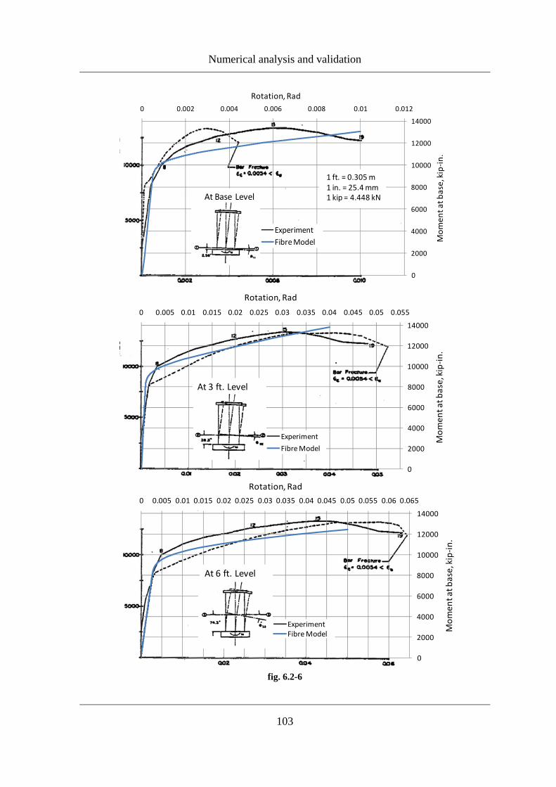
Numerical analysis and validation
103
0
2000
4000
6000
8000
10000
12000
14000
0 0.002 0.004 0.006 0.008 0.01 0.012
Mom
ent at b
ase, kip‐in
.
Rotation, Rad
ExperimentFibre Model
1 ft. = 0.305 m1 in. = 25.4 mm1 kip = 4.448 kNAt Base Level
0
2000
4000
6000
8000
10000
12000
14000
0 0.005 0.01 0.015 0.02 0.025 0.03 0.035 0.04 0.045 0.05 0.055
Mom
ent at b
ase, kip‐in
.
Rotation, Rad
Experiment
Fibre Model
At 3 ft. Level
0
2000
4000
6000
8000
10000
12000
14000
0 0.005 0.01 0.015 0.02 0.025 0.03 0.035 0.04 0.045 0.05 0.055 0.06 0.065
Mom
ent at b
ase, kip‐in
.
Rotation, Rad
ExperimentFibre Model
At 6 ft. Level
fig. 6.2-6

Chapter 6
104
0
10
20
30
40
50
60
70
80
0 0.005 0.01 0.015 0.02 0.025 0.03 0.035 0.04 0.045
Load, kips
Shear distortion, Rad
Experiment
Fibre Model
1 ft. = 0.305 m1 in. = 25.4 mm1 kip = 4.448 kN
In Base to 3 ft Level
0
10
20
30
40
50
60
70
80
0 0.005 0.01 0.015 0.02 0.025 0.03 0.035 0.04 0.045
Load, kips
Shear distortion, Rad
Experiment
Fibre Model
In 3 to 6 ft Level
0
10
20
30
40
50
60
70
80
0 0.005 0.01 0.015 0.02 0.025 0.03 0.035 0.04 0.045
Load, kips
Shear distortion, Rad
Experiment
Fibre Model
In Base to 6 ft Level
fig. 6.2-7
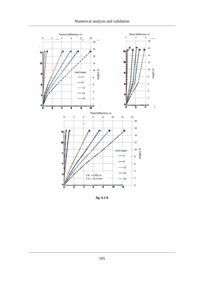
Numerical analysis and validation
105
0
2
4
6
8
10
12
14
16
18
0 2 4
Height, ft.
Shear Deflection, in.
0
2
4
6
8
10
12
14
16
18
0 2 4 6 8 10
Height, ft.
Flexure Deflection, in.
5
8
12
14
16
Load stages
0
2
4
6
8
10
12
14
16
18
0 2 4 6 8 10 12 14
Height, ft.
Total Deflection, in.
5
8
12
14
16
Load stages
1 ft. = 0.305 m1 in. = 25.4 mm
fig. 6.2-8

Chapter 6
106
6.3 Numerical comparison with VecTor2
The proposed model was tested also through various comparisons with other models,
implemented in available computer programs. This paragraph illustrates an example of a
comparison with the computer code VecTor2, based on bi-dimensional finite elements and
on MCFT constitutive law. The example regards a squat RC wall whose geometric
characteristics are shown in fig. 6.3-1. The adopted material properties are: concrete
cylinder compressive strength equal to 25 MPa and steel yielding stress equal to 450 MPa.
Web reinforcements are bars with a diameter equal to 8 mm at a spacing equal to 20 cm,
pillars reinforcement are 4 bars with a diameter equal to 16 mm. The proposed model was
applied considering for this structure 7 finite elements with 2 control sections per element
and 23 fibres per section fig. 6.3-2
Fibre subdivision of cross-section
(a) (b) fig. 6.3-2
P
5000 mm
7000
mm
5000 mm
250
mm
fig. 6.3-1
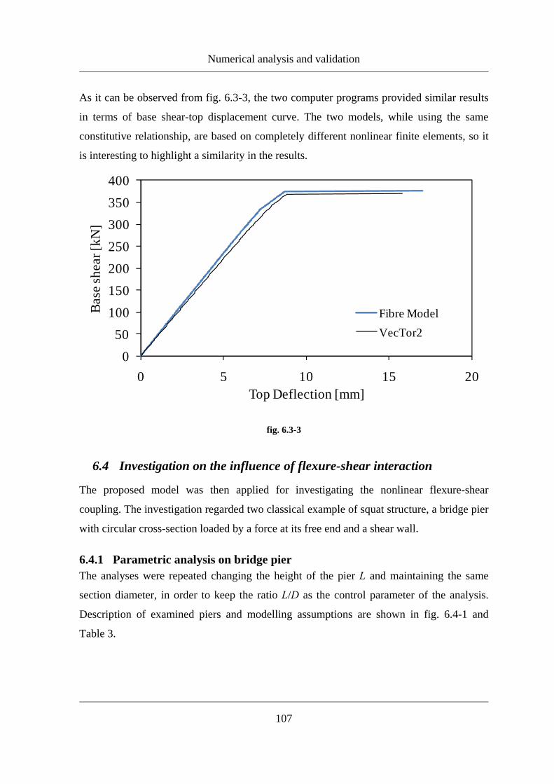
Numerical analysis and validation
107
As it can be observed from fig. 6.3-3, the two computer programs provided similar results
in terms of base shear-top displacement curve. The two models, while using the same
constitutive relationship, are based on completely different nonlinear finite elements, so it
is interesting to highlight a similarity in the results.
6.4 Investigation on the influence of flexure-shear interaction
The proposed model was then applied for investigating the nonlinear flexure-shear
coupling. The investigation regarded two classical example of squat structure, a bridge pier
with circular cross-section loaded by a force at its free end and a shear wall.
6.4.1 Parametric analysis on bridge pier The analyses were repeated changing the height of the pier L and maintaining the same
section diameter, in order to keep the ratio L/D as the control parameter of the analysis.
Description of examined piers and modelling assumptions are shown in fig. 6.4-1 and
Table 3.
050
100150200250300350400
0 5 10 15 20
Base
shea
r [kN
]
Top Deflection [mm]
Fibre ModelVecTor2
fig. 6.3-3

Chapter 6
108
Table 3. Geometrical dimensions and modelling assumptions of RC piers under study
Diameter (m) 2 2 2 2 2 2 2 2 2 2
Height (m) 2 4 6 8 10 12 14 16 18 20
L/D 1 2 3 4 5 6 7 8 9 10
Number of
elements 2 4 5 6 7 8 8 9 10 11
Element length
(m) 1.00 1.00 1.20 1.33 1.42 1.50 1.75 1.77 1.80 1.81
With regard to mechanical properties of materials, a concrete with cylinder compressive
strength equal to 45 MPa and a steel with yielding stress equal to 430 MPa were
considered. For each L/D ratio, two types of analysis were made: one considering
nonlinear flexural behaviour and linear shear response, uncoupled by the flexural one; the
other considering coupled nonlinear flexural and shear behaviour.
By calling with dMV the top displacement associated to the base shear at yielding and
calculated considering nonlinear flexure-shear interaction, and with dM the same type of
displacement obtained by keeping linear the shear behaviour, the results of the parametric
analysis are illustrated in fig. 6.4-2. In the Figure the ratio dMV/dM is plotted as a function of
the ratio L/D. This graph shows that nonlinear flexure-shear interaction affected the
response in a significant way for values of L/D lower than 4.
P
D = 2000 mm
L
D = 2000 mm
123 mm
φ24 mm
Fibre subdivision
(a) (b)
fig. 6.4-1

Numerical analysis and validation
109
In fig. 6.4-3 VM is the value of base shear calculated considering linear shear behaviour
while VMV is the value of base shear obtained considering nonlinear shear behaviour.
Figure 19 illustrates the ratio VM/VMV calculated at fixed values of top displacement in the
non-linear range and plotted as a function of the ratio L/D. This diagram shows again the
importance of nonlinear shear response. The inclusion of shear deformation, in fact,
increases the flexibility of the structure with the consequence that for obtaining given
displacement values, lower values of lateral load are required. In the range of L/D between
2 and 4 the obtained values of the ratio VM/VMV are around 1.15.
0.00
2.00
4.00
6.00
8.00
10.00
12.00
0 2 4 6 8 10
L/D
d M V /d M
fig. 6.4-2
fig. 6.4-3
0.95
1.00
1.05
1.10
1.15
1.20
1.25
0 2 4 6 8 10
L/D
V M / V MV
Displacement = 10 mm
Displacement = 40 mm
Displacement = 60 mm
Displacement = 80 mm

Chapter 6
110
fig. 6.4-4 illustrates the diagrams of base shear versus shear deformation evaluated at
different locations along the height of the pier. This graph shows that the shear response
changes along the height when nonlinear flexure-shear interaction is included in the
analysis. On the other hand the diagram of base shear versus shear deformation remains
linear and constant along the height when linear shear response is considered. Since shear
forces are constant along the height while diagrams of shear versus shear deformation does
change, it is clear also in these investigations, as noticed in the experimental results, that
the variation of bending moment along the height affects the shear deformations. This
result highlights the influence of flexure-shear interaction in the nonlinear response.
0
2000
4000
6000
8000
10000 Shear [KN]
fig. 6.4-4

Numerical analysis and validation
111
6.4.2 Parametric analysis on a shear wall This analysis was carried out, similar to the previous on a shear wall. Numerical results are
obtained keeping the section (reported in fig. 6.4-5) and varying the height. The main
analysis and results are reported below:
6.4.3 Analysis with the ratio L = 10d
(slender shear wall).
The wall was schematized with 20 elements (21 nodes). The geometrical discretization
and mechanical characteristics of the wall are reported in of the analysis are shown in
P
A A
L
Sez A-A
1000 mm
100 mmm
Ø 16 Ø8/100 mm
fig. 6.4-5
Steel
Concrete
fig. 6.4-6

Chapter 6
112
From the analysis the following diagrams are obtained. In red curve is represented the
flexural model keeping shear in linear elastic range, in blu curve a full copling between
flexure and shear is considered. The results are reported in terms of pushover curve,
moment curvature and shear-shear distortion.
Flexural model
Flexure-shear interaction
Pushover curve
Displacement [mm]
Shear [N]
fig. 6.4-7

Numerical analysis and validation
113
Flexural model
Flexure-shear interaction
Moment-curvature at the base
Curvature [mm-1]
Moment
[Nmm]
fig. 6.4-8

Chapter 6
114
Also in this example we can observe the capacity of the model to catch the flexure-shear
interaction, in particular is observed how the bending moment affects the T γ− diagram.
In fact the diagram shear-shear distortion varies along the height of the beam, even though
the shear is obviously constant on the wall.
Flexural model Flexure - shear interaction
Flexural model Flexure-shear interaction
Flexural model Flexure- shear interaction
Flexural model Flexure- shear interaction
Shear distortion Shear distortion
Shear distortion x 10-5 Shear distortion
x 10-5
x 10 4 x 104
x 10 4 x 104
x 10-5 x 10⁻⁵
Shear-shear distortion at the base Shear-shear distortion at node 5
Shear-shear distortion at node 10 Shear-shear distortion at node 15
fig. 6.4-9
Shear [N]
Shear [N]
Shear [N]
Shear [N]

Numerical analysis and validation
115
Stresses evaluated in earlier load steps
Stresses evaluated in latter load steps
Num
ber of fibre
Num
ber of fibre
Num
ber of fibre
Num
ber of fibre
6.4-10

Chapter 6
116
6.4.4 Analysis with the ratio L = 2d
.
In this second example, the wall was schematized with 4 nodes and 5 elements.
Geometrical and mechanical characteristics of the analysis are shown in 6.4-11
The results are presented in terms of pushover curve, moment curvature, shear-shear
distortion in the following figures 6.4-12; 6.4-13; 6.4-14:
Flexural model
Flexure-shear interaction
Displacement [mm]
Pushover curve
Shear [N]
6.4-12
Steel
Concrete
6.4-11

Numerical analysis and validation
117
Flexural model
Flexure-shear interaction
Moment
[Nmm]
6.4-13Curvature [mm-1]
Flexural model
Flexure-shear interaction
Shear[N]
Shear distortion
Shear-shear distortion at the base
6.4-14
Moment-curvature at the base

Chapter 6
118
6.4.5 Analysis with the ratio L = 1d
.
In this example the wall was schematized with 3 node and 2 elements. Mechanical and
geometrical parameters are represented below in fig 6.4-15:
Errore. L'origine riferimento non è stata trovata.
Steel
Concrete
6.4-15
Flexural model
Flexure-shear interaction
Shear [N]
Displacement [mm]
6.4-16
Pushover curve

Numerical analysis and validation
119
Flexural model
Flexure-shear interaction
Moment-curvature at the base
Moment
[Nmm]
Curvature [mm-1]6.4-17
Flexural model
Flexure-shear interaction
Shear-shear distortion at the base
Shear[N]
Shear distortion 6.4-18

Chapter 6
120
It may be observed that in a squat wall much as it analyzed in latter example, the non-
linear flexure-shear interaction will be decisive in determining the general behavior of the
structure. It may also notice that before cracking the two models return identical results.
This suggests that the model developed with flexure-shear interaction in non-linear field is
an extension of the simplest flexure element.

CHAPTER 7
Alternative formulation for the shear critical beam-column
element (developed in University of California Berkeley)
7.1 Sommario
Una formulazione alternativa a quella proposta fino ad ora è stata studiata presso
l'Università della California di Berkeley (UCB) sotto la supervisione del professor Filip. C
Filippou. L'elemento è stato sviluppato e implementato nella piattaforma informatica
FedeasLab (Saritas, Filippou (2006)). Per quanto riguarda il campo di spostamento, l’
elemento segue l'ipotesi della teoria della trave deformabile per taglio di Timoshenko,
mentre per la derivazione della risposta elemento è stato utilizzato una formulazione
variazionale a tre campi basata sul funzionale di Hu-Washizu. Il problema dei grandi
spostamenti è considerato attraverso l'uso della formulazione corotazionale.
Invece di un legame costitutivo bidimensionale per ogni fibra, è stato direttamente
utilizzato un modello tridimensionale del materiale in cui è stata successivamente applicata
una condensazione delle variabili attraverso l'equilibrio trasversale della sezione. Questo
garantisce l'accoppiamento delle tensioni in ogni sezione di controllo. Per lo stesso
elemento finito sono state introdotti due diversi legami costitutivi tridimensionali, uno per
le strutture in l'acciaio ed un altro per l'analisi di strutture in cemento armato.
Per il calcestruzzo è stato implementato un modello di danno con due parametri, uno per
controllare i danni in compressione e un altro parametro per il danno in trazione. Il modello
di danno tridimensionale utilizzato è stato formulato da Lee e Fenves (1998). Le pagine
seguenti descrivono in dettaglio la formulazione dell’ elemento finito e le relazioni
costitutive per il calcestruzzo e l'acciaio.
Validazioni ed analisi con il modello presentato nel seguente capitolo, sono tutt’ora in
corso, in particolare si tanno svolgendo confronti tra i due modelli presentati nella tesi.

CHAPTER 7
122
7.2 Finite element formulation
The finite element model under study is a two-dimensional beam formulated with the
assumption of small displacements, but large displacements and therefore non-linear
geometry can be considered and took into account in the transformation of the element
response from the local to the global reference system, through the corotational
formulation, as shown by Souza (2000) and Filippou and Fenves (2004).
7.2.1 Kinematic assumptions
The simplest beam theory including shear deformations in the structural response is the
Timoshenko beam theory based on the following displacement field:
( , ) ( ) - ( )( , ) ( )
x
y
u x y u x y xu x y w x
θ= ⋅=
(7.2.1)
Where θ (x) is the rotation of the normal to the undeformed x-axis, the normal to the
section does not coincide with the axis of the deformed beam.
In a single field variational formulation, the nodal displacements are generally assumed as
primary variables, and the interpolation functions of displacements are used to derive the
overall response of the element. If instead, a functional approach based on a two or three
fields is considered, in addition to the interpolation functions for displacements, are
required interpolation functions for tension (2 fields) or tension and the deformations (3
fields). These elements are generally more accurate and numerically stable in the non-
linear fields. The element presented is based on the latter approach, the element was
derived from the three functional fields, also known as Hu-Washizu functional, in which
was then introduced the kinematic assumption (7.2.1)
7.2.2 Hu-Washizu Functional
The mathematical formulation of the elastic element is based on the three fields, tension σ,
strain ε and displacement u, and is represented by the following equation:
( , , ) ( T U
HW extW d dΩ Ω
⎡ ⎤Π = ) Ω+ − Ω+Π⎣ ⎦∫ ∫σ ε u ε σ ε ε (7.2.2)
W(ε) is the strain energy function from which stresses are derived by

Alternative formulation for the shear critical beam-column element
123
( )Wσ ∂( ) =
∂εεε
(7.2.3)
ε U is the strain vector that is compatible with the displacements u according to this
equation:
s= ∇ε u (7.2.4)
Under small strains it is equal to the symmetric part of the displacement gradient s∇ . extΠ
is the energy associated with external forces, is expressed by the equation:
* *
t u
T T Text d d d
Ω Γ Γ⎡ ⎤Π = − Ω− Γ − − Γ⎣ ⎦∫ ∫ ∫u b u t t u u
(7.2.5)
Where t = σ ∙ n and n is the normal to the boundary, * superscript denotes the imposed
values of variables. It is assumed that the external loading is conservative so that the work
depends only on the final displacement values u. Ω is the domain of the free body which
are associated volume forces, while Γt Γu are the loaded and bounded surfaces respectively
to which are associated surface forces or imposed displacements.
The formulation of the beam obtained using a three-field functional, allows for the
independent specification of the strains ε from the displacements u. This allow the
selection of section kinematic independent from beam kinematics. Introducing the beam
kinematic described in equation (7.2.1) in equation (7.2.4) the following equation can be
written:
( , ) '( ) '( )
( , )( , ) ) '( )
u xxx
yu xxy
du x y u x y xdx
du x ydu x y x w xdy dx
ε θ
γ θ
= = − ⋅
= + = − ( + (7.2.6)
The section strain field is taken in accordance with the following relation.
( ) )
, ) ( )xx a
xy
x y xy z x
ε ε κγ φ γ
− (⎧ ⎫ ⎧ ⎫= =⎨ ⎬ ⎨ ⎬(⎩ ⎭⎩ ⎭
ε (7.2.7)
Where ( )a xε is the axial deformation along the x-axis, )xκ( is the curvature and ( )xγ is the
section shear strain. In this model can be introduced a non uniform shear strain of the
section through the function , )y zφ( . In this function was introduced a simplification,
considering it a function of y only, instead y and z , ) )y z yφ φ( ≡ ( .
Writing the functional (7.2.2) for the beam, the following can be written:

CHAPTER 7
124
ˆ T u T uHW extd d dδ δ δ δ δ δ
Ω Ω Ω⎡ ⎤ ⎡ ⎤Π = ( ) Ω+ − Ω+ − Ω+ Π⎣ ⎦ ⎣ ⎦∫ ∫ ∫σ ε ε σ ε ε σ ε ε (7.2.8)
substituting (7.2.6) and (7.2.7) in (7.2.8) results:
( ) ( ) ( ) ( ) [ ] ( ) ( ) [ ]
ˆ ˆ( ) ) ) ( )
'( ) ) ' ) ( )
'( ) ) ) ( )
'( ) ) ' ) ( )
'( ) ) ) ( )
HW xx a xy
xx a
xx
xx a
xx ext
x y x y x d
u x x y x x d
w x x y x d
u x x y x x d
w x x y x d
δ σ δε δκ σ φ δγ
δσ ε θ κ
δσ θ φ γ
σ δ δε δθ δκ
σ δ δθ φ δγ δ
Ω
Ω
Ω
Ω
Ω
Π = − ( + ( Ω +
− ( − ( − Ω+⎡ ⎤⎣ ⎦
− ( − ( Ω+
− ( − ( − Ω+⎡ ⎤⎣ ⎦
− ( − ( Ω + Π
∫∫∫∫∫
(7.2.9)
Section forces are defined as follow:
)
xx xx xyA A A
xyA
N dA M y dA V dA
and V y dA
σ σ σ
φ σ
= = − =
= (
∫ ∫ ∫∫
(7.2.10)
Where N is the axial force, M is the bending moment, V is the shear force and V* that is
work conjugate with the shear strain field , ) ( )y z xφ γ( of the equation (7.2.7). From
equations (7.2.10), the equation (7.2.9) become:
( ) ( ) ( )
( ) ( ) ( )
( )
* *
0
*
0
0
ˆ ˆ ˆ( ) ) )
'( ) ( ) '( ) ( ) '( ) ( ) )
'( ) '( ) '( ) )
l
HW a
l
a
l
ext
x N N x M M x V V dx
u x x M x x V w x x V x dx
u x N x M w x x V dx
δ δε δκ δγ
δ ε δ θ κ δ θ δ γ
δ δθ δ δθ
Π = − + ( − + ( − +
+ Ν − + − + − − ( +
+ + + − ( +Π
∫
∫
∫
(7.2.11)
Where
ˆ ˆ ˆˆ ˆ ˆ
ˆ ˆ)
xx xx xyA A A
xyA
N dA M y dA V dA
and V y dA
σ σ σ
φ σ
= = − =
= (
∫ ∫ ∫∫
(7.2.12)
The potential energy of the external loads can be written as follow:
0
( ) ( ) ( ) ( ) )l
ext n x u x q x w x m x x dxδ δ δ δθΠ = − + ( ) + (∫ (7.2.13)
Whose quantity are represented in the following figure fig.7.2-1:
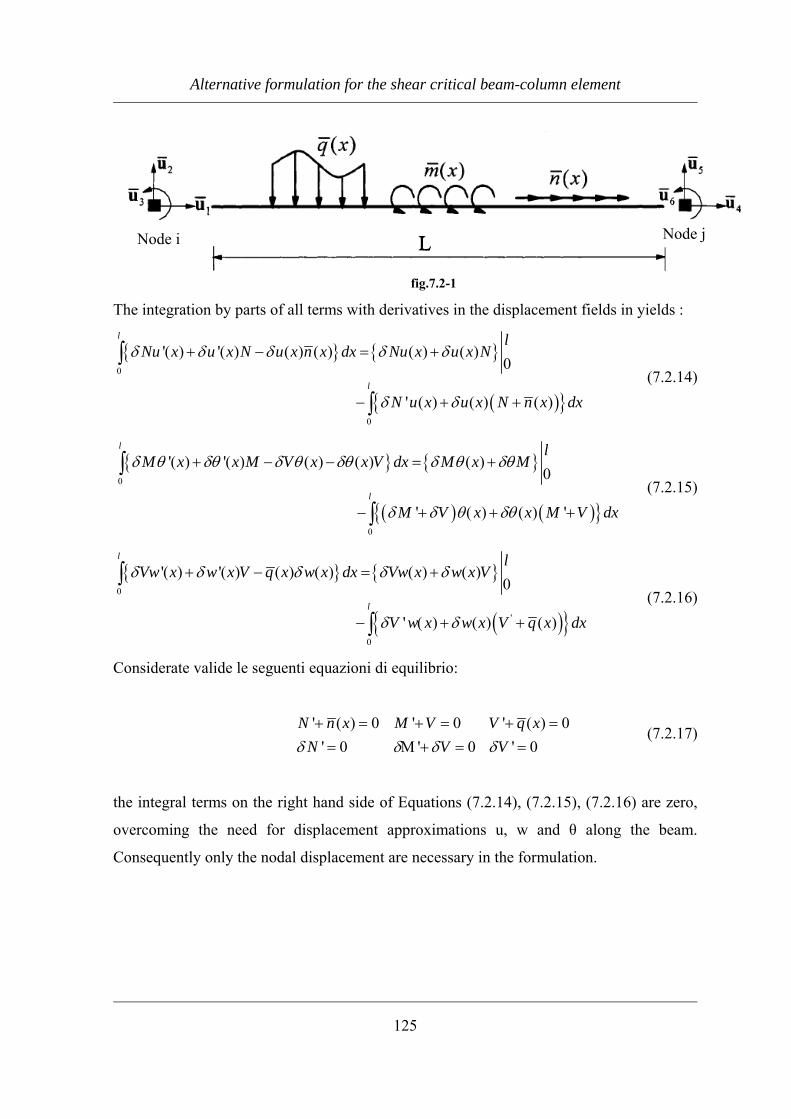
Alternative formulation for the shear critical beam-column element
125
The integration by parts of all terms with derivatives in the displacement fields in yields :
( ) 0
0
'( ) '( ) ( ) ( ) ( ) ( )0
' ( ) ( ) ( )
l
l
lNu x u x N u x n x dx Nu x u x N
N u x u x N n x dx
δ δ δ δ δ
δ δ
+ − = +
− + +
∫
∫ (7.2.14)
( ) ( ) 0
0
'( ) '( ) ( ) ( ) ( )0
' ) ( ) '
l
l
lM x x M V x x V dx M x M
M V x x M V dx
δ θ δθ δ θ δθ δ θ δθ
δ δ θ δθ
+ − − = +
− + ( + +
∫
∫ (7.2.15)
( ) 0
'
0
'( ) '( ) ( ) ( ) ( ) ( )0
' ) ( ) ( )
l
l
lVw x w x V q x w x dx Vw x w x V
V w x w x V q x dx
δ δ δ δ δ
δ δ
+ − = +
− ( + +
∫
∫ (7.2.16)
Considerate valide le seguenti equazioni di equilibrio:
' ( ) 0 ' 0 ' ( ) 0' 0 ' 0 ' 0
N n x M V V q xN V Vδ δ δ δ+ = + = + == Μ + = =
(7.2.17)
the integral terms on the right hand side of Equations (7.2.14), (7.2.15), (7.2.16) are zero,
overcoming the need for displacement approximations u, w and θ along the beam.
Consequently only the nodal displacement are necessary in the formulation.
Node i Node j
fig.7.2-1
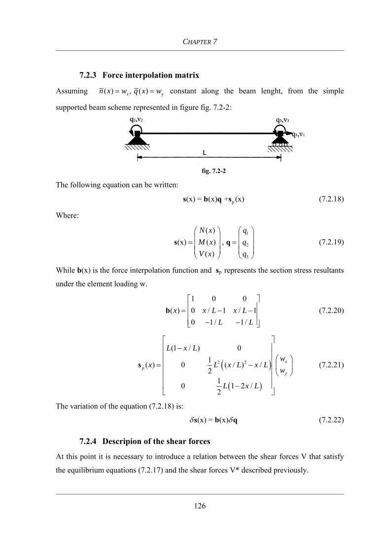
CHAPTER 7
126
7.2.3 Force interpolation matrix
Assuming ( ) , ( )x yn x w q x w= = constant along the beam lenght, from the simple
supported beam scheme represented in figure fig. 7.2-2:
The following equation can be written:
p(x) = (x) + (x)s b q s (7.2.18)
Where:
1
2
3
( )(x) ( ) ,
( )
N x qM x qV x q
⎛ ⎞ ⎛ ⎞⎜ ⎟ ⎜ ⎟= =⎜ ⎟ ⎜ ⎟⎜ ⎟ ⎜ ⎟⎝ ⎠ ⎝ ⎠
s q (7.2.19)
While b(x) is the force interpolation function and sp represents the section stress resultants
under the element loading w.
1 0 0
( ) 0 / 1 / 10 1/ 1/
x x L x LL L
⎡ ⎤⎢ ⎥= − −⎢ ⎥⎢ ⎥− −⎣ ⎦
b (7.2.20)
( )
( )
2 2
(1 / ) 01( ) 0 ( / ) /2
10 1 2 /2
xp
y
L x Lw
x L x L x Lw
L x L
⎡ ⎤⎢ ⎥−⎢ ⎥ ⎛ ⎞⎢ ⎥= − ⎜ ⎟⎢ ⎥ ⎝ ⎠⎢ ⎥⎢ ⎥−⎣ ⎦
s (7.2.21)
The variation of the equation (7.2.18) is:
(x) = (x)δ δs b q (7.2.22)
7.2.4 Descripion of the shear forces
At this point it is necessary to introduce a relation between the shear forces V that satisfy
the equilibrium equations (7.2.17) and the shear forces V* described previously.
fig. 7.2-2

Alternative formulation for the shear critical beam-column element
127
To find a relationship between V and V*, it is assumed the hypothesis of linear elastic
material, for which the following equation can be written:
* 2
)( ( ))
) ) ( ( ))
xyA A
xyA A
V dA y G x dA
V y dA y G x dA
σ φ γ
φ σ φ γ
= = (
= ( = (
∫ ∫
∫ ∫ (7.2.23)
Therefore, this relationship can be expressed as follows:
2
*
)in cui
)A
A
y dAV V
y dA
φβ β
φ
(= =
(
∫
∫ (7.2.24)
Substituting (7.2.24) in the functional, combining the parameter β with the deformation
( )xγ , modified deformation can be founded as follow:
( ) ( )x xγ β γ= ⋅ (7.2.25)
In the functional the this equation can be written:
*ˆ ˆ) )x V x Vδγ δγ( = ( (7.2.26)
therefore:
( )ˆ ) in cui )xyA
yV y dA y φψ σ ψβ
= ( ( =∫ (7.2.27)
7.2.5 Section deformation and stiffness matrix
The kinematics of the section is described by the following equation:
( )
1 0)
0 0 ))
axx
sxy
xy
xy
x
εε
ε κγ ψ
γ
⎡ ⎤−⎛ ⎞ ⎡ ⎤ ⎢ ⎥= = ⋅ = ⋅ (⎜ ⎟ ⎢ ⎥ ⎢ ⎥(⎣ ⎦⎝ ⎠ ⎢ ⎥(⎣ ⎦
a e (7.2.28)
The section forces can be expressed by the following equations:
ˆˆ 1 0 ˆˆˆ ˆ 0 ˆˆ 0 ( )
ˆ)
xxA
xxxx
xyA A
xyA
dAN
M y dA y dAyV
y dA
σ
σσ
σψ
ψ σ
⎛ ⎞⎜ ⎟⎛ ⎞ ⎜ ⎟ ⎡ ⎤⎜ ⎟ ⎡ ⎤⎜ ⎟ ⎢ ⎥= = − = − ⋅⎜ ⎟ ⎢ ⎥⎜ ⎟ ⎢ ⎥⎜ ⎟ ⎣ ⎦⎜ ⎟ ⎢ ⎥⎜ ⎟ ⎣ ⎦⎝ ⎠ ⎜ ⎟(⎜ ⎟⎝ ⎠
∫
∫ ∫
∫
s (7.2.29)

CHAPTER 7
128
The derivative of section forces, with respect to the section deformations defined in results
in the section tangent stiffness matrix
ˆ ˆ ( )T T
s s s mA A
dA dAδ δ εδ δ
= = =∫ ∫s σk a a k ae e
(7.2.30)
Where mk is the tangent modulus, defined as ˆ ( )
mδ εδ
=σkε
Considering a fibre discretization of the section, the section stiffness matrix can be
obtained by the following summation.
, , ,
2, , ,
1 2, , ,
))
) ) )
aa i aa i i sa in
s aa i i aa i i i sa i ii
i sa i i i sa i i ss i
k y k y ky k y k y y k Ay k y y k y k
ψψ
ψ ψ ψ=
⎡ ⎤− ⋅ (⎢ ⎥= − ⋅ − ( ⋅⎢ ⎥⎢ ⎥( − ( (⎣ ⎦
∑k (7.2.31)
where n is the number of fibre of the section.
Once known the section stiffness matrix, the element stiffness matrix is obtained by
integration, than the structural stiffness matrix is assembled by classical method.
7.3 Constitutive relationships.
The finite element described in the formulation can be used to simulate concrete and steel
structures. To catch the flexure-shear coupling, a multi axial bond must be used, at least a
bidimensional relationship. For steel structures has been implemented a classical plasticity
model, while for concrete a three-dimensional approach based on the damage model,
proposed by Lee and Fenves (1998), is used. To adjust a three-dimensional model in a
beam element has been introduced a static condensation. This procedure is carried out
considering the stirrups as a translational constraint, or introducing the hypothesis of a
plane stress state if stirrups are not present.
7.3.1 Steel material model
To model steel structures, was used a general J2 plasticity model as a constitutive
relationship , presented by Lubliner et al. (1993) improved by Auricchio and Taylor
(1995). This model, compared to the classical Prandtl-Reuss J2, has the advantage of
considering the material hardening through the expansion of the yield surface.
In this plasticity model are defined two type of function, one limit function F and one
yield function F, the latter is the same function as that used in classical plasticity theory.

Alternative formulation for the shear critical beam-column element
129
The function F distinguishes between admissible and inadmissible states, and provides a
smooth transition between elastic and inelastic states. This behaviour is much more
realistic for metallic materials. Graphically, this kind of model can be represented by the
following figure in case of uniaxial material.
The function F is classically defined as:
2F J k= − (7.2.32)
Where J2 is defined as the second invariant of the deviatoric stress tensor while F is
defined as follow:
( ) :FF h F δ λδ
⎛ ⎞= ⋅ −⎜ ⎟⎝ ⎠
σσ
(7.2.33)
where λ is called consistency parameter and must satisfies the following
loading/unloading conditions:
, 0 0F e Fλ λ≥ 0 ≤ = (7.2.34)
( )h F is defined as follow:
( ) ( ); i k
Fh F H H HF Hδ ϕ ϕ
= = +− +
(7.2.35)
where φ is the distance between the current and the asymptotic radius of the yield function
and δ is the rate of approaching the asymptote. Booth are the constants that define the
connection between the curves.
Hi is the isotropic hardening modulus and Hk is the kinematics hardening modulus.
fig. 7.3-1

CHAPTER 7
130
For further information about this plasticity model of can be found in Lubliner et al. (1993)
Auricchio and Taylor (1995).
7.3.2 Concrete material model
Concrete has shown the stress-strain behavior of a plastic material as well as that of a
material with damage. For this reason several models proposed to combine the two
theories. Lubliner et al. (1989) developed a plastic-damage model that is easier to calibrate
with experimental data. However, Lee and Fenves (1994) show that the relation between
the degradation variables and the plastic strain lead to a complex and unstable algorithm.
Lee and Fenves (1998) developed a plastic-damage model with two damage variables, one
for a tensile and one for a compressive damage state, and modified the yield function of the
Barcelona model to include the two damage variables. Lee and Fenves (1998) plastic-
damage model is the basis on which the concrete constitutive relationship is developed.
This choice arises from the fact that the concrete has the behavior of a plastic material
although it is certainly subjected to cyclic damage. Compared to the model presented in
Lee and Fenves’s articles, the derivation of the tangent modulus of the material has been
changed. In the following will be briefly explained the damage model used.
According to the plasticity theory, the strain tensor can be divided into two parts, one
elastic and one plastic, as follow:
( )0p= −σ C ε ε (7.2.36)
0C is the initial elastic stiffness. The plastic strain rate is determined with a flow rule in
connection with a plastic potential function Ф according to this relation:
)p δλδΦ(
=σεσ
(7.2.37)
In the original Lee and Fenves (1998) model a single internal damage variable κ is
introduced, which is assumed to satisfy the following damage evolution rule
( , )λ=κ H σ κ (7.2.38)
Lubliner et al. (1989) use a single damage variable, this variable is a combination of tensile
and compressive damage variables. This assumption is accurate only for monotonic

Alternative formulation for the shear critical beam-column element
131
loading. Lee and Fenves introduce two damage variables, one for compression and the
other for tensile state. This hypothesis makes the behavior more realistic in the case of
cyclic loading. The damage variables are taken as follow:
t
c
κκ⎧ ⎫
= ⎨ ⎬⎩ ⎭
κ (7.2.39)
Tensile and compression strength are functions of the damage parameters:
( ) ( ),t t t c c cf f f fκ κ= = (7.2.40)
According to the classical damage mechanics this relation can be written:
1 D
=−σσ (7.2.41)
Where σ represent the effective stress and D is a positive scalar parameter, that can
assume values between 0 (undamaged material) ad 1 (broken material). From the definition
the following equation can be deduced:
( ) ( ) ( ) ( )1 , 1t t t t t c c c c cf D f f D fκ κ κ κ= − = −⎡ ⎤ ⎡ ⎤⎣ ⎦ ⎣ ⎦ (7.2.42)
where ( ) ( )0 1, 0 1t t c cD Dκ κ≤ ≤ ≤ ≤ . A single damage parameter can be derived by the
two parameters above:
( ) ( )( )1 1 1t cD D D Dκ= = − − − (7.2.43)
The limit surfaces proposed initially by Lubliner and subsequently modified by Lee and
Fenves is effective for every type of loading, as shown in numerous analysis, except for an
hydrostatic loading, for which the problem of never reach the crisis.
The limit surface concerned is represented by the following equation:
( ) ( )1 2 max1 ˆ3
1 cF I J cα β σα
= + + −−
σ (7.2.44)
Where maxσ is the algebraically largest principal stress, I1 is the first invariant of the
hydrostatic stress tensor and J2 is the second invariant of the deviatoric stress tensor, α is a
dimensionless parameter, expressed in terms of the initial uniaxial compressive yield stress
fc0 and the initial biaxial compressive yield stress fb0, according to:
0 0
0 02b c
b c
f ff f
α −=
− (7.2.45)

CHAPTER 7
132
β is the Barcellona constant, which is found in the homonymous model (Lubliner (1989)).
Lee and Fenves have changed the parameter β as follows:
( ) ( )( ) ( )( )1 1c
t
CC
β β α α= = − +κ
κκ
(7.2.46)
Where ( ) ( ),c c c t t tC f C f= − =κ κ are cohesion values in tension and compression,
respectively.
An important aspect to consider is the static condensation of the stiffness matrix , obtained
for a three-dimensional material, on a beam column element. To this end, the constraints
have been imposed considering the effect of shear reinforcement (stirrups), according to
the following equilibrium equation:
00
yy y yyy
zz z z
fRfRz
σ ρσ ρ
+⎧ ⎫⎧ ⎫ ⎧ ⎫= = =⎨ ⎬ ⎨ ⎬ ⎨ ⎬+⎩ ⎭ ⎩ ⎭⎩ ⎭
R (7.2.47)
Where , without shear reinforcement 0y zρ ρ= = the equation (7.2.47) returns the case of
plane stress state condition. Linearizing (7.2.47) with respect to an initial strain 0ε in the y
direction gives:
( ) ( )0 ,0
0
yy yy yyyy y y y xx yy zz
xx yy zz
yy yy yy yxy yz xz y yy
xy yz xz yy
f
f
σ σ σσ ε ρ ε ε ε ε
ε ε ε
σ σ σγ γ γ ρ ε
γ γ γ ε
∂ ∂ ∂+ + Δ + Δ + Δ +
∂ ∂ ∂
∂ ∂ ∂ ∂+ Δ + Δ + Δ + Δ =∂ ∂ ∂ ∂
(7.2.48)
In z direction similarly:
( ) ( )0 ,0
0
zz zz zzzz z z z xx yy zz
xx yy zz
zz zz zz zxy yz xz z zz
xy yz xz zz
f
f
σ σ σσ ε ρ ε ε ε εε ε ε
σ σ σγ γ γ ρ εγ γ γ ε
∂ ∂ ∂+ + Δ + Δ + Δ +
∂ ∂ ∂
∂ ∂ ∂ ∂+ Δ + Δ + Δ + Δ =∂ ∂ ∂ ∂
(7.2.49)
In writing the linearized equations, it was considered that for a planar beam, the shear
deformations are zero 0, 0yz xzγ γ= = as well as their increments 0, 0yz xzγ γΔ = Δ = .
The equations (7.2.48) and (7.2.49) can be written in matrix form as follow:
,0
,0
xxyyyy y y yyzz yyxx yyxy yyxzyyy
xyzzyy zzzz z z zzxx zzxy zzxzzzz
xz
C E C C C CRC C E C C CR
ερ ε
γρ ε
γ
Δ⎧ ⎫+ Δ⎡ ⎤ ⎡ ⎤⎧ ⎫⎧ ⎫ ⎪ ⎪= − − Δ⎨ ⎬ ⎨ ⎬ ⎨ ⎬⎢ ⎥ ⎢ ⎥+ Δ⎩ ⎭ ⎩ ⎭⎣ ⎦ ⎣ ⎦ ⎪ ⎪Δ⎩ ⎭
(7.2.50)
Alternative formulation for the shear critical beam-column element
133
The incremental stress-strain relation, can be written separating the normal strains in the transverse direction:
xx xxxx xxxy xxxz xx xxyy xxzz
yyxy xyxx xyxy xyxz xy xyyy xyzz
zzxz xzxx xzxy xzxz xz xzyy xzzz
C C C C CC C C C CC C C C C
σ εε
σ γε
σ γ
⎡ ⎤ ⎡ ⎤Δ Δ⎡ ⎤ ⎧ ⎫Δ⎧ ⎫⎢ ⎥ ⎢ ⎥⎪ ⎪⎢ ⎥Δ = Δ +⎨ ⎬ ⎨ ⎬⎢ ⎥ ⎢ ⎥⎢ ⎥ Δ⎩ ⎭⎪ ⎪⎢ ⎥ ⎢ ⎥⎢ ⎥Δ Δ⎣ ⎦ ⎩ ⎭⎣ ⎦ ⎣ ⎦
(7.2.51)
substituting the (7.2.51) in (7.2.50) for the converged state R=0 (transverse equilibrium),
the condensed material stiffness matrix can be obtained
1xxxx xxxy xxxz xxyy xxzzyyyy y y yyzz yyxx yyxy yyxz
m xyxx xyxy xyxz xyyy xyzzzzyy zzzz z z zzxx zzxy zzxz
xzxx xzxy xzxz xzyy xzzz
C C C C CC E C C C C
C C C C CC C E C C C
C C C C C
ρρ
−⎡ ⎤ ⎡ ⎤⎛ ⎞+⎡ ⎤ ⎡ ⎤⎢ ⎥ ⎢ ⎥= − ⎜ ⎟⎢ ⎥ ⎢ ⎥⎢ ⎥ ⎢ ⎥ ⎜ ⎟+⎣ ⎦ ⎣ ⎦⎝ ⎠⎢ ⎥ ⎢ ⎥⎣ ⎦ ⎣ ⎦
k (7.2.52)
The same procedure can be used considering only two stress components xxσ e xyσ .

CONCLUSION
This thesis illustrates the attempt to introduce a model that can accurately reproduce the
nonlinear behavior of structures where shear deformation is critical for the overall
behaviour. In a fibre beam-column element based on flexibility formulation a constitutive
relationship that allows to reproduce the nonlinear flexure-shear interaction was introduced
for the purpose. Indeed in this category of elements there aren’t still models, of proven
accuracy, able to reproduce the squat structures behaviour. The main characteristics of the
beam-column element are substantially two:
• The flexibility formulation, based on the two-fields mixed method
• The constitutive relationship based on the MCFT, in which a rotating smeared-
crack bidemensional model is assumed for the concrete.
While the fibre model considered is based on the incremental load approach and tangent
stiffness matrix, the modified compression field theory on which the constitutive relation is
based, considers a total load approach and secant stiffness matrix for the iterations.
In particular was chosen to adapt the original MCFT to an algorithm based on the
incremental load approach and the tangent stiffness matrix to take advantage of the more
fast convergence resulting from this approach. The algorithm includes an element state
determination, well established for flexibility based elements, and a new section state
determination, with iterations at the fibre level for the determination of the stress and
strains in concrete and steel according to the constitutive model.
The proposed model was implemented in an original computer code and then calibrated
and validated through comparisons with available experimental results.
The verification regarded in particular some tests conducted by Osterele et al(1979) on RC
walls for which the different contributions to the deflected shape due to flexure and shear
were available. The results shown that The model was able to simulate accurately these
contributions at different levels of excursion in the inelastic range. The results were carried
out in terms of Pushover curve, moment-rotation, shear- shear deformation and deformed
shape.
A further test was carried out through numerical comparisons with the computer program
VecTor2, based on bi-dimensional finite elements and on MCFT constitutive law. The
analysis was carried out on a shear wall fixed at the base and loaded by a force on top.

Conclusion
135
Although the two codes are based on two different types of finite elements, the results
obtained in global terms, that is in terms of pushover curve are comparable. Even
numerical comparisons have shown that the proposed model can be effectively used, in the
monotonic loading, for the analysis of squat structures.
Various numerical analyses were then performed in order to study the influence of flexure-
shear interaction. First of all a bridge pier with circular cross section was analyzed to
investigate this kind of influence, the analyses were repeated changing the height of the
pier and maintaining the same section diameter, in order to keep the slenderness as the
control parameter of the analysis. Than an similar analysis was carried out un a shear wall
in which the slenderness range was between one and ten. From these analyses it is evident
the influence of the nonlinear shear deformation, especially for the elements characterized
by a ratio of length to section dimension lower than 4. The observed variation along the
element of the shear response, associated to the variation of bending moment, highlights
the influence of flexure-shear interaction in the inelastic range and the capability of the
model in reproducing this effect.
The implementation of the MCFT constitutive relationship in a fibre beam-column model
seemed to be a proper solution for the simulation of shear dominated elements in the
nonlinear range. The inclusion of shear response however involved a significant increase
of the complexity of the algorithm of the fibre model. The presented applications of the
model regard analyses in presence of monotonic loading. More research work is required at
the date to extend the applications for cyclic loading.
As regards to the model studied in the University of California Berkeley has been reported
the finite element formulation based on a three fields functional and the constitutive laws
for concrete and steel structures. Between the two models presented are still in progress
studies and comparisons, which will be reported in future papers.
With regard to the first model presented in this thesis, the following future developments
can be highlighted:
• Implementation of a cyclic analysis, changing from a load control to a displacement
control. This allows to capture effects such as softening, fundamental in nonlinear
analysis of reinforced concrete structures

Conclusion
136
• Simplification of the constitutive relationship, with the aim of reducing the levels of
iteration and therefore the computational time.
• The future extension of the model should account for a more accurate distribution
of shear strains over the section, until now assumed constant.
• Finally The beam finite element model can be extended to include the interaction of
axial force, biaxial bending moment, biaxial shear and torsion through the 3d
coupling of normal and shear stresses. A warping function for torsion must be
added to the kinematic assumptions.
As regard to the second model studied at University of California Berkeley, the following
developments are underway:
• Numerical validation and comparisons between the two models, first in monotonic
than in cyclic loading
• Implementation of Biaxial constitutive relationship as Modified Compression Field
theory, in the Timoshenko beam element formulated on three-field Hu-Washizu
variational.

REFERENCES
Bairan, J.M. (2005). “A Nonlinear Coupled Model for the Analysis of Reinforced Concrete
Sections Under Bending, Shear, Torsion and Axial Forces.”, Ph.D. thesis, Technical
University of California, Barcelona, Spain.
Banon, H., Biggs, J. e Irvine, M.(1981). “Seismic Damage in Reinforced Concrete
Frames”. Journal of Structural Engineering, ASCE, 107(ST9), p.p. 1713-1729.
Bentz, E.C. (2000). “Sectional Analysis of Reinforced Concrete Member.”, Ph.D. thesis,
Technical University of Toronto, Canada.
Brancaleoni, F., Ciampi, V. e Di Antonio, R (1983). “Rate Type Models for Nonlinear
Hysteretic Structural Behaviour.” EUROMECH Colloquium, Palermo Italia
Ceresa P., Petrini L., Pinho R. (2007). “Flexure-shear fibre beam-column elements for
modelling frame structures under seismic loading - state of the art.” Journal of Earthquake
Engineering, Vol. 11, Special Issue 1.
Ceresa P., Petrini L., Pinho R. e Auricchio F.(2007). “ Development of a Flexure-Shear
Fibre Beam-Column Elements for Modelling of Frame Structures Under Seismic
Loading.” First European Conference on Earthquake Engineering and Seismology,
Geneva, Switzerland 2006, paper number 1425
Cervenka, V. (1985). “Constitutive Models for Cracked Reinforced Concrete.” ACI
journal, 82(6),877-882.
Cloug , R. e Benuska, L. (1966). “Nonlinear Earthquake Behaviour of Tall Buildings.”
Journal of Mechanical Engineering, ASCE, 93(EM3), 129-146.
Clough, R. and Johnston, (1967). “Effect of Stiffness Degradation on Earthquake Ductility
Requirements.” Transactions of Japan Earthquake Engineering Symposium, Tokyo, p.p.
195-198.

References
138
Crisfield, M.A. (1986 ). “Snap-Through and Snap-Back response in concrete structure and
the danger of under-interaction”, International Journal of Numerical Methods in
Engineering, 22, 751-767.
Darvall, L.P. e Mendis, P. (1985). “Elastic-Plastic- Softening Analysis of Plane Frames”,
Journal of Structural Engineering, ASCE, 11 (STA4), 871-888.
Filippou, F.C. e Issa, A. (1988). “Nonlinear Analysis of Reinforced Concrete Frames
under Cyclic Load Reversal”, EERC Report 83-19, Earthquake Engineering. Research
Centre, Berkeley.
Taucer F.F. , Spacone E. e Filippou F.C., (1991). “A Fiber Beam-Column Element
for Seismic Response Analysis of Reinforced Concrete Structures”, EERC Report 91-17,
Earthquake Engineering Research Centre, Berkeley.
Spacone, E. e Taucer, F.F., Filippou, F.C. (1996). “A Fiber Beam-Column Model for
Nonlinear Analysis of R/C Frames: Part.1 Formulation” Earthquake Engineering and
Structural Dynamics 25, 711-725
Giberson, M. (1967). “The Response of Nonlinear Multi-Story Structures Subjected to
Earthquake Excitation”. Earthquake Engineering Research Laboratory, Pasadena.
Guedes, J. e Pinto, A.V. (1997). “A Numerical Models for Shear Dominates Bridges
Piers”, Proceedings of the Second Italy-Japan Workshop on Seismic Design and Retrofit of
Bridges, Rome, Italy.
Guedes , J., Pegon, P. e Pinto, A.V.(1994-1997). “A Fiber-Timoshenko Beam Element in
CASTEM 2000”, Special publication Nr. 1.94.31 Applied Mechanics Unit, Safety
Technology Institute, Commission of European Communities, Joint Research Centre, Ispra
Establishment, Italy

References
139
Guner S, Vecchio FJ. Pushover Analysis of Shear-Critical Frames: Formulation. ACI
Structural Journal 2010; 107: 63-71.
Lai, S. Will, G. e Otani, S. (1984). “Model for Inelastic Biaxial Bending of Concrete
Members”. Journal of Structural Engineering, ASCE, 110(ST11), 2563-2584.
Mander, J.B., Priestley, M.J.N. e Park, R. (1988). “Theoretical Stress-Strain Model for
Confined Concrete”. Journal of Structural Engineering, ASCE, 114(ST8), 1804-
1826.
Martinelli, L. (1998-2002) “Modellazione di Pile da Ponte in C.A. a travata soggetti ad
eccitazione sismica”, Phd. thesis, Dipartimento di Ingegneria Strutturale, Politecnico
di Milano, Milano, Italy
Mazars, J. Kotronis, P., Ragueneu, F. e Casaux, G. et al. (2006). “Using Multifiber Beams
to Account for Shear and Torsion. Application to Concrete Structural Element”,
Computer Methods in Applied Mechanics end Engineering 195(52), 7264-7281.
Meyer, C., Roufaiel, M.S. and Arzoumanidis, S.G.(1983). “Analysis of Damaged Concrete
Frames for Cyclic Loads”, Earthquake Engineering and Structural Dynamics,
vol.11, 207- 228.
Meyer, C., Roufaiel, M.S. (1987). “Analytical Modelling of Hysteretic Behaviour of R/C
Frames”, Journal of Structural Engineering, ASCE, 113(ST3), 429-444.
Otani, S. (1974). “Inelastic Analysis of R/C Frame Structure”, Journal of the Structural
Division, ACSE, 100(ST7).
Oesterle G, Fiorato AE, Johal LS, Carpenter JE, Russsell HG,(1974) Corley WG.
Earthquake resistant structural walls – Tests of isolated walls. Report to National
Science Foundation, 1976, Submitted by Research and Construction Technology
Laboratories, Portland Cement Association, Illinois.

References
140
Petrangeli, M, Pinto, P. e Ciampi, V.(1996,1999). “Fiber Element for Cyclic Bending and
Shear of R/C Structures. I: theory”, Journal of Engineering and Mechanics
125(9), 994,1001.
Ranzo, G. e Petrangeli, M. (1998). “A Fiber Beam Element with Section Shear Modelling
for Seismic Analysis of R/C Structures “, Journal of Earthquake Engineering 2, 443-
473
Remino, M. (2004). “Shear Modelling of Reinforced Concrete Structures”, Phd. Thesis,
Dipartimento di Ingegneria civile, Università degli studi di Brescia, Brescia, Italia.
Rose, B.W. (2001). “A Constitutive Model for the Analysis of reinforced concrete beams-
columns subjected to lateral loads”, Phd. Thesis, CEAE Dept., University of
Colorado, Boudler, Colorado.
Saiidi M., Sozen M. A. (1981) “Simple Nonlinear Seismic Analysis of R/C Structures”,
Journal of the Structural Division, ASCE, 107 (ST5)
Saritas A, Filippou FC. (2009) “Inelastic axial-flexure–shear coupling in a mixed
formulation beam finite element.” International Journal of Non-Linear Mechanics;
44: 913-922.
Selby, R.G., Vecchio, F.J. (1991). “Towards Compression-Field Analysis of Reinforced
Concrete Solids” Journal of Structural Engineering, ASCE, 117(6), 1740-1758.
Soleimani, D., Popov, E.P. e Bertero, V.V. (1979). “Nonlinear Beam Model for R/C Frame
Analysis”, 7th ASCEE Conference of Electronic Computation, St. Louis.
Takayanagi, T. e Schnobrich, W. (1979) . “Nonlinear Analysis of Coupled Wall
Systems”, Earthquake Engineering and Structural Dynamics, vol.7, 1-22.

References
141
Takeda, T., Sozen, M.A. e Nilsen, N. (1970). “Reinforced Concrete Response to Simulated
Earthquakes”, Journal of Structural Engineering, ASCE, 96(ST12), 2557-2573.
Takizawa, H. e Aoyama, H. (1976). “Biaxial Effects in Modelling Earthquake Response of
R/C Structure”, Trans. of Arch. Inst. of Japan , 240, Part.1 in Feb. 1976, pp. 51-62,
Part. 2 in March 1976, pp. 65-77.
Vecchio, F.J., Collins, M.P. (1986). “ The Modified Compression Field Theory for
Reinforced Concrete Element Subjected to Shear”, Journal of American Concrete
Intitute, 83(2), 219-231.
Vecchio, F.J., Collins, M.P. (1988). “Predicting the Response of Reinforced Concrete
Beams Subjected to Shear Using the Modified Compression Field Theory”, ACI
Structural Journal, 85,258-268.
Vecchio, F.J.(2000). “Disturbed Stress Field Model of Reinforced Concrete: Formulation”,
Journal of Structural Engineering, ASCE, 126(9), 1070-1077.
Vecchio, F.J.(2001). “Disturbed Stress Field Model of Reinforced Concrete:
Implementation”, Journal of Structural Engineering, ASCE, 127 (1), 12-20.
Walraven, J. C. (1981). “Fundamental analysis of aggregate interlock.” Journal of
Structural Engineering, ASCE, 107(11), 2245–2270.
Wong P, Vecchio FJ. (2003) VecTor2 and Formworks Manual.
http://www.civ.utoronto.ca/vector/, .
Zeris, C.A. e Mahin, S.A. (1988). “Analysis of Reinforced Concrete Beam-Column under
uniaxial Excitation”, Journal of Structural Engineering, ASCE, 114(ST4), 804-820.

References
142
Zienkiewicz, O.C. e Taylor, R.L (1989). The Finite Element Method. Vol. I. Basic
Formulation and Linear Problems. Fourth Edition, McGraw Hill, London.
Zienkiewicz, O.C. e Taylor, R.L (1989). The Finite Element Method. Vol. II. Solid and
Fluid Mechanics, Dynamics and Non-Linearity. Fourth Edition, McGraw Hill,
London.