A Semiparametric Estimation for Regression Functions … and Masry (2000) propose an additive...
19
573 Available at http://pvamu.edu/aam Appl. Appl. Math. ISSN: 1932-9466 Vol. 9, Issue 2 (December 2014), pp. 573-591 Applications and Applied Mathematics: An International Journal (AAM) A Semiparametric Estimation for Regression Functions in the Partially Linear Autoregressive Time Series Model R. Farnoosh and M. Hajebi Department of Mathematics Iran University of Science and Technology Tehran 16846, Iran [email protected]; ibejahm@msui.ea.mi S.J. Mortazavi Department of Mathematics Islamic Azad University of Science and Research Branch Tehran, Iran [email protected] Received: May 19, 2014; Accepted: October 2, 2014 Abstract In this paper, a semiparametric method is proposed for estimating regression function in the partially linear autoregressive time series model. Here, we consider a combination of parametric forms and nonlinear functions, in which the errors are independent. Semiparametric and nonparametric curve estimation provides a useful tool for exploring and understanding the structure of a nonlinear time series data set to make for a more efficient study in the partially linear autoregressive model. The unknown parameters are estimated using the conditional nonlinear least squares method, and the nonparametric adjustment is also estimated by defining and minimizing the local L2-fitting criterion with respect to the nonparametric adjustment and, with smooth-kernel method, these estimates are corrected. Then, the autoregression function estimators, which can be calculated with the sample and simulation data, are obtained. In this case, some strong and weak consistency and simulated results for the semiparametric estimation in this model are presented. The root mean square error and the average square error criterions are also applied to verify the efficiency of the suggested model. Keywords: Semiparametric estimation; Nonparametric adjustment; Conditional nonlinear least squares method; Partially linear autoregressive model; Smooth kernel approach; Autocorrelation function; Simulation MSC 2010 No.: C14, C15, C52, C53
Transcript of A Semiparametric Estimation for Regression Functions … and Masry (2000) propose an additive...

573
Available at
http://pvamu.edu/aam Appl. Appl. Math.
ISSN: 1932-9466
Vol. 9, Issue 2 (December 2014), pp. 573-591
Applications and Applied
Mathematics:
An International Journal
(AAM)
A Semiparametric Estimation for Regression Functionsin the
Partially Linear Autoregressive Time Series Model
R.Farnoosh and M.Hajebi
Department of Mathematics
Iran University of Science and Technology
Tehran 16846, Iran
[email protected]; [email protected]
S.J.Mortazavi Department of Mathematics
Islamic Azad University of Science and
Research Branch
Tehran, Iran
Received: May 19, 2014; Accepted: October 2, 2014
Abstract
In this paper, a semiparametric method is proposed for estimating regression function in the
partially linear autoregressive time series model. Here, we consider a combination of parametric
forms and nonlinear functions, in which the errors are independent. Semiparametric and
nonparametric curve estimation provides a useful tool for exploring and understanding the
structure of a nonlinear time series data set to make for a more efficient study in the partially
linear autoregressive model. The unknown parameters are estimated using the conditional
nonlinear least squares method, and the nonparametric adjustment is also estimated by defining
and minimizing the local L2-fitting criterion with respect to the nonparametric adjustment and,
with smooth-kernel method, these estimates are corrected. Then, the autoregression function
estimators, which can be calculated with the sample and simulation data, are obtained. In this
case, some strong and weak consistency and simulatedresults for the semiparametric estimation
in this model are presented. The root mean square error and the average square error criterions
are also applied to verify the efficiency of the suggested model.
Keywords: Semiparametric estimation; Nonparametric adjustment; Conditional nonlinear
least squares method; Partially linear autoregressive model; Smooth kernel
approach; Autocorrelation function; Simulation
MSC 2010 No.: C14, C15, C52,C53
574 R. Farnoosh et al.
1. Introduction
The nonlinear autoregressive models are the most popular models for the nonlinear time series
analysis. Over the past two decades, there has been a growing interest in the time series literature for
nonlinear models [Tong (1990)]. Several authors have constructed nonlinear time series models shown to
be useful in some applications. Haggen and Ozaki (1981) propose the exponential autoregressive model
to apply in the modeling of sound vibration. Cai and Masry (2000) propose an additive nonlinear ARX
time series model to consider the estimation and identification of components, both endogenous and
exogenous. Chen and Tsay (1993) propose a class of nonlinear additive autoregressive models with
exogenous variable for nonlinear time series analysis. Farnoosh and Mortazavi (2011) propose the first-
order nonlinear autoregressive model with dependent errors to estimate the yearly amount of deposits in
an Iranian Bank.
In time series analysis with the focus on autoregressive models, one faces, in particular, three
problems: model identification, i.e., lag selection, model estimation and prediction. Many
methods have been proposed to cope with these problems. For nonlinear models, there are results
showing the strong (or weak) consistency and asymptotic normality of the estimators.
Semiparametric and nonparametric curve estimation provides a useful tool for exploring and
understanding the structure of a nonlinear time data set, especially when classic time series
models are inappropriate. Auestad and Tjostheim (1990) applied a multivariate kernel smoothing
method to estimate the conditional mean and conditional variance of a nonlinear autoregression.
Our interest is the estimation of parameters in a nonlinear time series model which is usually
performed by conditional least squares. Achievement of nice asymptotic properties of these
estimators is not automatic because of the diverse possibilities in the choice of the model. Results
for conditional least squares estimators are proved in Klimko and Nelson (1978) in a general set
up. In this paper, we intend to propose a combination of parametric forms and nonlinear
functions to make a more efficient study in the following partially linear autoregressive model
( ) | | ( )
At first, we suppose that f(.) has a parametric framework, namely parametric model as
( ) * ( ) + ( )
where ( ) is a known smooth function of x, and 𝜖 is a parametric space. Both and β
are unknown parameters.
We suggest a semiparametric form ( ) ( ) for the unknown autoregression function
f(.), where ( ) is a nonparametric adjustment. This model is a simple generalization of the first-
order nonlinear autoregressive model of Jones (1978) and Zhuoxi et al. (2009), and is a time
series counterpart of the generalized additive model of Hastie and Tibshirani (1990) in regression
analysis that was introduced by Gao (1998), Gao and Yee (2000).
The goal of this paper is to extend the work of Zhuoxi et al. (2009) in the semiparametric
estimation for the nonlinear autoregressive model. There are a number of practical motivations
behind it; these include the search for population biology models and the Mackey-Glass system

AAM: Intern. J., Vol. 9, Issue 2 (December 2014) 575
[see Glass and Mackey (1988))]. In addition, the recent development in partially linear
(semiparametric) regression (see Heckman (1986); Hardle et al. (1997)) has established a solid
foundation for studying model (1.1).
We want to estimate f(x) and ( ) under the following form
( ) ( ) ( ) ( )
Hence, we use a combination of parametric method and nonparametric adjustment. The
parameters and nonparametric adjustment are estimated, using a conditional nonlinear least
squares method and then, with the smooth-kernel method, these estimates are corrected, so it will
be considered as
( ) ( ) ( ) ( )
The contents of this paper are organized as follows. In section 2, a conditional nonlinear least
squares method is presented to estimating parameters and β. Also, in this section, the
semiparametric estimator is introduced by a natural consideration of the local L2-fitting criterion
for the partially linear autoregressive time series model. The strong and weak consistencies of
the semiparametric estimations are investigated in section 3. The performance of this method is
assessed by simulation in section 4. Finally, section 5 illustrates an application of this model to
predict annual ring width (ARW), of Kelardasht site in the north of Iran, from 1974 to 2008.
2. Semiparametric estimation in the partially linear autoregressive time
series model
We consider the following model
( ) | | ( )
where { } is a sequence of independent and identically-distributed (i.i.d) random variables with
mean zero and variance . Also, and are independent for each t and β is unknown
parameter.We want to estimate the regression function f(x) that can be formed as ( ), where
( ) is afunction of x with as an unknown parameter of the model. For the model
(2.1), and β should be well estimated withconditional nonlinear least squares errors method as
follows
( ) ∑{( ( ))
} ( )
and
( ) ( ) | | ( )
In fact, and are the common conditional least squares estimators based on ,

576 R. Farnoosh et al.
for n successive observations from the model.
Now, we estimate ( ) in ( ) ( ) ( ) by using a similar idea of Hjort and Jones (1996),
Zhuoxi et al. (2009) and Farnoosh and Mortazavi (2011).
We define the local L2-fitting criterion asthe following form
( ) ∑ (
)* ( ) ( ) +
( )
where f(.) is an unknown autoregression function with sample size n, k is a kernel and is
band- width. So we obtain the estimator ( ) of ( ) by minimizing theabove criterion with
respect to ( ). Therefore, we get a nonparametric estimator with smooth kernel method of
( ) as
( ) ∑ [ (
) ( ) ( )]
∑ [ (
) ( )]
( )
then the estimator of f(x) could be
( ) ( ) ( ) ( )
Unfortunately, the formula ( ) contains the unknown functionf(x), therefore by using
( )
and with regard to the fact the errors of model are small values, we have
∑ (
) ( ) ( ) ∑ (
) ( )( )
Therefore, one can obtain
( ) ∑ [ (
) ( )( )]
∑ [ (
) ( )]
( )
Finally, the autoregression function estimators which can be calculated with the sample and
simulation data, are
( ) ( ) ( ) ( )

AAM: Intern. J., Vol. 9, Issue 2 (December 2014) 577
3. The assumptions and properties of asymptotic behaviors
In this section, some properties and the asymptotic behaviors of theestimator are investigated.
The assumptions A1-A10 are considered as follows
(A1) f(.) is Lipschitz continuous and all moments of are finite and the density function of
errors is Lipschitz and bounded total variation, also, the sequence * + is stationary
ergodic sequence of integrable random variable. See Hayashi (2000) and Taniguchi and
Kakizawa (2000).
(A2)
exist and are continuous, for all
where i,j,k =1,..., m.
(A3) ( | ) ( | )
where k is a constant.
(A4) We define
( ) ( | ) ( )
and the following matrices
( ( )
( )
)
( ( )(
( )
( )
))
We will assume throughout that B and D are positive definite and finite.
(A5) The sequence ( ) is α-mixing (Yu (1973)). The sufficient conditions are
introduced. See Rosenblatt (1971), Bradley (2007), Masry and Tjostheim (1995) and
Robinson (1983).
(A6) and have the same distribution π(.), such that the density φ(.) of π(.) exists,
bounded, continuous and strictly positive in aneighborhood of the point x.
(A7) ( ) and ( ) are bounded and continuous with respect to x, away from 0 in a
neighborhood of the point x.Set ( ) ( )
(A8) ( ) has continuous derivative with respect to and the derivative at the point is
uniformly bounded with respect to x.

578 R. Farnoosh et al.
(A9) The kernel k: is a compactly symmetric bounded function, such that ( ) for x in a set of positive Lebesgue measures.
(A10) where
If we accept assumptions (A1)-(A10), we have the following lemma and theorems:
Lemma 3.1.
Under the conditions (A1)-(A10), We have the following results when .
( ) ∑ (
) ( ) ( )
( ) ( ) ( )
( ) ∑ (
) ( )
( )
( )
where ( ) is defined as in (A7) and φ(x) is the density of or which is bounded,
continuous and strictly positive in aneighborhood of the point x.
Proof ( ):
It can be calculated as
∑ (
) ( ) ( )
*∑ (
) ( ( ) ( )) ( )
+
∑ (
) ( ) ( )
Using (A1)-(A4), and strong consistency of the conditional least squares method Klimko and
Nelson(1978), and (A7)-(A9), we have
|( ( ) ( )) ( )| (( ) )
Since, f(x) and k(x) are bounded and continuous with respect to x, one can claim: there exists
such that
|∑ (
) ( ( ) ( )) ( )
AAM: Intern. J., Vol. 9, Issue 2 (December 2014) 579
∑ | ( ) ( )|
|
((
) ) (( )
)
Thus, a.s. as
Due to the sequence * + is α-mixing, then
∑ (
) ( ) ( )
{ (
) ( ) ( )}
as
According to (A6)-(A7), we can show (Put u=
also,∫ ( ) * ( )+)
{ (
) ( ) ( )}
∫ (
) ( ) ( ) ( )
∫ ( ) ( ) ( ) ( )
( ) ( ) ( )∫ ( )
Therefore,
∑ (
) ( ) ( )
( ) ( ) ( )
as
Proof (b):
Since, ( ) is bounded and continuous with respect to x, ta ai
∑ (
) ( )
*∑ (
) ( ( ) ( )) ( )
+
∑ (
) ( ) ( )
580 R. Farnoosh et al.
Using (A8)-(A10), there exists , such that
| | ∑
| ( ) ( )|
(( ) )
(( )
)
Thus, a.s. as
According to (A5), the sequence * + is α-mixing, therefore
∑ (
) ( ) ( )
{ (
) ( )}
According to (A6)-(A7),we can show (Put
,also, ∫ ( ) * ( )+)
{ (
) ( )}
∫ (
) ( ) ( ) ( )
∫ ( ) ( ) ( )
Finally,
∑ (
) ( ) ( )
( )
( )
as
Therefore, the proof is complete.
Theorem 3.2.
If we accept the assumptions (A1)-(A10) and ( ) be the introduced estimator in (2.6), then
( ) ( ) as

AAM: Intern. J., Vol. 9, Issue 2 (December 2014) 581
Proof:
Substituting Lemma 3.1 in (2.6) and using the strong consistency of and we canprove
Theorem 3.2.
Theorem 3.3.
If we accept the assumptions (A1)-(A10) and ( ) be the defined autoregression function
estimator in(2.8), then ( ) ( ) as
Proof:
One may obtain the equality
( ) ( ) ( )∑ [ (
) ( )]
∑ [ (
) ( )]
On the other hand, we have
∑ [ (
) ( )]
∑ [ (
) ( ( ) ( ))]
∑ [ (
) ( )]
To complete the proof, it is known that
| | (( ) )
a.s., as it is enough to show and
, as
It follows that
|
∑ * (
) ( ( ) ( ))+
|
∑ [ | || ( ) ( )|]
(( )
) ((
) ) ((
) )

582 R. Farnoosh et al.
which implies a.s., as
Since
* ∑ [ (
) ( )]
+
and
* ∑ [ (
) ( )]
+
,∑ [ (
) ( )]
-
,∑ [ (
)
( )]
-
∑ [ (
) ( ) (
) ( )]
(
)
where is a constant, we get By the strong consistency of and
and lemma 3.1, we complete the proof.
4. Simulation Study
We investigate the appropriateness of semiparametric method by estimating parameters and
regression function in the following model
( )
tith ( ( ) ) where * + is a sequence of independent identically-distributed (i.i.d)
random variables. We generate the data with sample sizes n=400,600,800 using the following
nonlinear functions
( ) ( )
and assume
( ) ( )

AAM: Intern. J., Vol. 9, Issue 2 (December 2014) 583
( ) ( ) ( )
and assume
( ) ( )
Finally, we compute the average square error (ASE) for the efficiency of the proposed estimation
method
∑ { ( ) ( )}
The square root of the ASE is denoted by RMSE (Root Mean Square Error).
Tables 1 and 2 show the descriptive statistics indices for simulation data and errors in the above
mentioned models 1 and 2, respectively. The Kolmogorov-Smirnov statistic is obtained to test
the normality of the errors of model. The test statistic and p-value confirm the normality of the
residuals. Also, the RMSE estimation for the above mentioned models 1 and 2 are provided in
Tables 3 and 4.
Figures 1 and 2 show the curves of f(x) and its semiparametric estimator under the two types of
the above mentioned models with selected bandwidth and different sample sizes. The red and
blue lines are the regression function f(x) and the semiparametric estimator respectively. Also,
Figures 3 and 4 show the autocorrelation function (ACF) errors of the model with f(x) and its
semiparametric estimator under the two types of above mentioned models with selected
bandwidth and different sample sizes.
These two figures, show that the ACF errors of the model are almost uncorrelated. The
simulation results show that the semiparametric estiamator of the autoregression function
performs well.
Table 1. Descriptive statisticsfor the simulation data and errors of the model ( )
var N Min Max Mean std K-
Smirnov
P-value
data 400 0.69 4.05 1.3178 0.88613 6.021 0.0000101
data 600 0.69 4.05 1.3104 0.87522 7.37 0.0000071
data 800 0.69 4.05 1.2392 0.77338 8.47 0.000048
error 400 0.4016 0.49 0.06 0.1511 1.128 0.157
error 600 -0.44 0.75 0.0592 0.1754 1.353 0.0865
error 800 -0.73 0.84 0.06 0.1911 1.421 0.0721

584 R. Farnoosh et al.
Figure 1. ( ) , n=600, RMSE=0.0725.
Table 2. Descriptive statisticsfor the simulation data and errors of the model ( ) ( ) var N Min Max Mean std K-Smirnov P-value
data 400 0.11 1.05 0.4093 0.2525 3.061 0.000146
data 600 0.11 1.05 0.4089 0.2523 3.748 0.000105
data 800 0.11 1.05 0.4087 0.2519 4.32 0.000091
error 400 -0.13 0.12 -0.004 0.04715 1.1755 0.126
error 600 -0.15 0.152 -0.002 0.03412 0.888 0.41
error 800 -0.121 0.17 -0.003 0.04431 1.238 0.092
Table 3. RMSE for estimating the model ( )
n RMSE
400 4.769153 0.523312 0.09 0.0806
600 5.2131 0.495932 0.112 0.0725
800 5.1771 0.472340 0.135 0.0643
Table 4. RMSE for estimating the model ( ) ( ) n RMSE
400 7.86 4.2137 0.3754 0.13219 0.0265
600 7.85 4.1943 0.3901 0.10538 0.0249
800 6.6987 4.1131 0.1077 0.1325 0.0142

AAM: Intern. J., Vol. 9, Issue 2 (December 2014) 585
Figure 2. ( ) ( ), n=600, RMSE=0.0249
Figure 3. ACF of errors of the model ( )
, n=600

586 R. Farnoosh et al.
Figure 4. ACF of errors of the model ( ) ( ) n=600
Figure 5. Exact values of ARW for three species (Pinus Eldarica) of Kelardasht site
(The north of Iran)
5. Empirical Application
In this research, three normal Pinus eldarica trees were randomly selected from a plantation at
Garagpas-Kelardasht site, which is located in the western part of the Mazandaran province in the
north of Iran. These treeshave grown for over 35 years in this site. TbaPinus eldarica Medw is
mixed with some Pinus sylvestris, Pinus nigra and Picea abies at the Garagpas-Kelardasht
site. The Pinus eldarica trees were cut for this studyin January 2009. To illustrate the suitability

AAM: Intern. J., Vol. 9, Issue 2 (December 2014) 587
of our methodology to the ARWdata, we use an additive functional autoregressive model to
forecast the ARW of kelardasht site in the north of Iran, from 1974 to 2008. The following
functional-autoregressive model is proposed as empirical model
( )
where { } is a sequence of i.i.d random variables with mean zero and variance . Also,
and are independent for each t and is constant. Using the presented semiparametric
method, we estimate the regression function.
Table 5, respectively, shows the observed-estimated value for the ARW data of kelardasht site in
the north of Iran, from 1974 to 2008. The descriptive statistics of the ARW of pine wood are
shown in Table 6. There are significant differences between the growth andring width (radius)
of a tree in a year. The ARW values were increasing by increasing age of tree (radial axis). The
mean of the ARW of three trees was 3.74 mm.
The RMSE and ASE values of the regression function for the functional autoregressive models
are shown in Table 7. Figure 5 shows the curves of the observations (the ARW data in threetrees
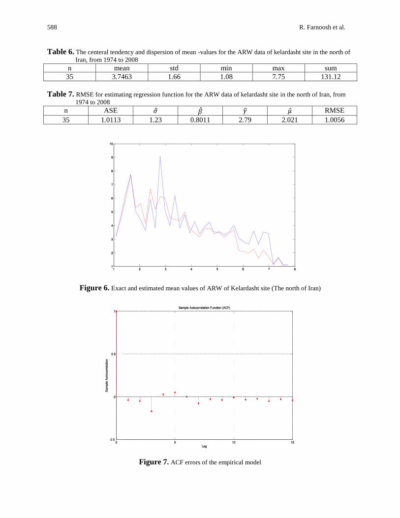
of Pinus Elderica) from 1974 to 2008. Figure 6 shows the curves of the observations (the mean
of ARW data) and its semiparametric estimator with selected bandwidth.
The red and blue lines are the curves of the observations and the semiparametric
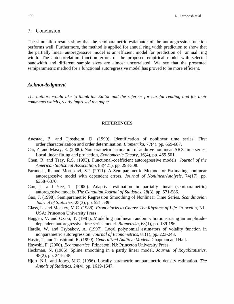
predictor, respectively. Figure 7 shows the ACF errors of the proposed empirical model. The
errors of themodel are almost uncorrelated. We see that the presented semiparametric method
for a functional autoregressive model is more efficient.
Table 5. The observed - forcasted mean -values for the ARW data of kelardasht site in the north of
Iran, from 1974 to 2008
Time Exact-value Forecasted-value Time Exact-value Forecasted-value 1974 3.17 3.21 1992 3.74 4.21
1975 4.43 4.39 1993 3.82 3.13
1976 5.91 6.30 1994 3.51 4.07
1977 7.75 7.73 1995 3.51 3.62
1978 5.30 3.52 1996 3.14 3.34
1979 5.68 3.90 1997 3.41 3.74
1980 4.14 4.91 1998 2.72 2.47
1981 6.71 5.39 1999 2.18 2.71
1982 5.18 5.83 2000 2.07 2.97
1983 6.12 8.34 2001 2.00 2.57
1984 6.03 6.66 2002 2.28 2.96
1985 4.59 4.87 2003 1.61 2.33
1986 4.43 4.47 2004 2.21 2.53
1987 4.36 6.33 2005 1.77 2.02
1988 5.03 4.47 2006 1.15 1.56
1989 3.80 6.64 2007 1.65 1.67
1990 3.45 3.51 2008 1.08 1.12
1991 3.18 3.02
588 R. Farnoosh et al.
Table 6. The centeral tendency and dispersion of mean -values for the ARW data of kelardasht site in the north of
Iran, from 1974 to 2008
n mean std min max sum
35 3.7463 1.66 1.08 7.75 131.12
Table 7. RMSE for estimating regression function for the ARW data of kelardasht site in the north of Iran, from
1974 to 2008
n ASE RMSE
35 1.0113 1.23 0.8011 2.79 2.021 1.0056
Figure 6. Exact and estimated mean values of ARW of Kelardasht site (The north of Iran)
Figure 7. ACF errors of the empirical model

AAM: Intern. J., Vol. 9, Issue 2 (December 2014) 589
6. Summary
The partially linear autoregressive model is currently used in a variety of fields, including
econometric studies, finance, wood industry science, biometrics, engineering, genetics, ecology
and biology. This paper proposed a combination of parametric forms and nonlinear functions, in
which the errors are independent. Theerrors and observations are also independent for each t.
Since the parametric methods are not very efficient to estimate the regression functions, semipar-
ametric methodsare used.
At first, we suppose that the regression function f(.) has a parametric framework, that can be
formed as ( ) where ( ) is a function of x with as an unknown parameter of the
model. Therefore, we suggested a semiparametric form ( ) ( ) for the unknown
autoregression function f(.), where ( ) is a nonparametric adjustment. The unknown parameters
are estimated using the conditional nonlinear least squares method and by defining and
minimizing the local L2-fitting criterion with respect to ( ), the nonparametric adjustment is
also estimated and then, with smooth-kernel method, these estimates are corrected. So, the
estimator of f(x) can be obtained. Because the formula ( ) contains the unknown function
f(x), and with regard to the fact the errors of the model are small values, we can obtain ( ) euea
estimator of ( )
In order to investigate the efficiency of the semiparametric method in our model, we consider an
empirical application. Hereby, three normal Pinus eldarica trees were randomly selectedfrom a
plantation at Garagpas-Kelardasht site, which is located in the western part of the Mazandaran
province in the north of Iran. These trees have grown over 35 years in this site. The Pinus
eldarica trees were cut for this studyin January 2009. The ARW Pinus eldarica was predicted by
an additive functional autoregressive model, from 1974 to2008. The results are shown in Tables
(5-7) and Figures (5-7) which indicate that the presented semiparametric method for a
functional autoregressive model is more efficient.
Table 5, respectively, shows the observed-estimated value for the ARW data of kelardasht site in
the north of Iran. In Table 6, the descriptive statistics of the ARW of pine wood isshown. We
see that there are significant differences between the growth andring width (radius) of a tree in a
year, so much so that the ARW values were increasing by increasing age of tree (radial axis).
The RMSE and ASE criterions are also applied to verify the efficiency of the suggested model.
The RMSE and ASE values of the regression function for the functional autoregressive models
are shown in Table 7. As we can see, it supports the iaeiefficiency of the suggested model.
The curves of the ARW data in threetrees of Pinus Elderica are shown in Figure 5. The curves of
the mean of ARW data and its semiparametric estimator with selected bandwidth are also shown
in Figure 6. Also, Figure 7 shows the ACF errors of the proposed empirical model which
indicates that the errors of themodel are almost uncorrelated. The results of the study show that
the semiparametric estiamator of the autoregression function performs well.
590 R. Farnoosh et al.
7. Coaalsumoa
The simulation results show that the semiparametric estiamator of the autoregression function
performs well. Furthermore, the method is applied for annual ring width prediction to show that
the partially linear autoregressive model is an efficient model for prediction of annual ring
width. The autocorrelation function errors of the proposed empirical model with selected
bandwidth and different sample sizes are almost uncorrelated. We see that the presented
semiparametric method for a functional autoregressive model has proved to be more efficient.
Acknowledgment
The authors would like to thank the Editor and the referees for careful reading and for their
comments which greatly improved the paper.
REFERENCES
Auestad, B. and Tjostheim, D. (1990). Identification of nonlinear time series: First
order characterization and order determination. Biometrika, 77(4), pp. 669-687.
Cai, Z. and Masry, E. (2000). Nonparametric estimation ofadditive nonlinear ARX time series:
Local linear fitting and projection, Econometric Theory, 16(4), pp. 465-501.
Chen, R. and Tsay, R.S. (1993). Functional-coefficient autoregressive models. Journal of the
American Statistical Association, 88(421), pp. 298-308.
Farnoosh, R. and Mortazavi, S.J. (2011). A Semiparametric Method for Estimating nonlinear
autoregressive model with dependent errors. Journal of NonlinearAnalysis, 74(17), pp.
6358–6370.
Gao, J. and Yee, T. (2000). Adaptive estimation in partially linear (semiparametric)
autoregrssive models. The Canadian Journal of Statistics, 28(3), pp. 571-586.
Gao, J. (1998). Semiparametric Regression Smoothing of Nonlinear Time Series. Scandinavian
Journal of Statistics, 25(3), pp. 521-539.
Glass, L. and Mackey, M.C.(1988). From clocks to Chaos: The Rhythms of Life. Princeton, NJ,
USA: Princeton University Press.
Haggen, V. and Ozaki, T. (1981). Modelling nonlinear random vibrations using an amplitude-
dependent autoregressive time series model. Biometrika, 68(1), pp. 189-196.
Hardle, W. and Tsybakov, A. (1997). Local polynomial estimators of volality function in
nonparametric autoregression. Journal of Econometrics, 81(1), pp. 223-243.
Hastie, T. and Tibshirani, R.(1990). Generalized Additive Models. Chapman and Hall.
Hayashi, F. (2000). Econometrics. Princeton, NJ: Princeton University Press.
Heckman, N. (1986). Spline smoothing in a partly linear model. Journal of RoyalStatistics,
48(2), pp. 244-248.
Hjort, N.L. and Jones, M.C. (1996). Locally parametric nonparametric density estimation. The
Annals of Statistics, 24(4), pp. 1619-1647.

AAM: Intern. J., Vol. 9, Issue 2 (December 2014) 591
Jones, D.A. (1978). Nonlinear Autoregressive Processes. Proceedings of the Royal Society of
London, Mathematical and Physical Sciences, 360(A), pp. 71-95.
Klimko, L.A. and Nelson, P.L. (1978). On conditional least square estimator for stochastic
processes. The Annals of Statistics, 6(3), pp. 629-642.
Masry, E. and Tjostheim, D. (1995). Nonparametric estimation and identification of nonlinear
ARCH time series: strong convergence and asymptotic normality. EconometricTheory,
11(2), pp. 258-289.
Rosenblatt, M. (1971). Markov processes, Structure and Asymptotic Behavior. Springer-Verlag,
Inc.
Bradley, R.C. (2007). Introduction to Strong Mixing Conditions. Kendrick Press, Heber City,
Utah, Volume 1, 2, 3.
Robinson, P.M. (1983). Nonparametric estimation for time series models. Journal of Time
Series Analysis, 4(3), pp. 185-208.
Taniguchi, M. and Kakizawa, Y. (2000). Asymptotic Theory of Statistical Inference for Time
Series. New York: Springer-Verlag NY.
Tong, H. (1990). Nonlinear Time Series. Oxford University Press, Oxford.
Yu, A.D. (1973). Mixing conditions for markov chains. Theory of Probability and itsApplic
ations, 18(2), pp. 312-328.
Zhuoxi, Y. Dehui, W. and Ningzhoneg, S. (2009). Semiparametric estimation of regression
function in autoregressive models. Journal of Statistics and Probability Letters, 79(2),
pp. 165-172.