SERI/TR-98372-1 UC CATEGORY: UC-61a

ANAEROBIC FERMENTATION OF BEEF CATTLE MANURE

FINAL REPORT

-A. G. HASHIMOTO Y. R. CHEN -V. H. VAREL

ROMAN L. HRUSKA U.S. MEAN ' ANIMAL , RESEARCH CENTER

U.S. DEPARTMENT OF AGRICULTURE CLAY CENTER, NEBRASKA

JANUARY 1981

PREPARED UNDER SUBCONTRACT No. 08-9-8372-1 FOR THE Solar Energy Research Institute A Division of Midwest Research Institute

1617 Cole Boulevard Golden, Colorado 80401

Prepared for the U,S, Department of. Energy Contract No, EG-77-C-01-4042

SERI TECHNICAL MONITOR:

DAN JANTZEN

FOREWORD

This report describes the results of a research project to produce energy in the form of methane and a high protein feed supplement from livestock manure. This work was jointly funded by the US Department of Agriculture, through the Science and Education Administration, and the US Department of Energy, through the Solar Energy Research Institute.

The results of this research indicates that there are many livestock operations where thermophillic fermentation of livestock manure would be both technically feasible and economically attractive. The develop­ment of this technology has now reached the point where a significant commercialization effort is needed, aimed at integrating such fermen­tation units into livestock production operations.

The USDA and DOE are currently working out arrangements for such a program.

~~ Senior Project Manager Biomass Program Office

i

SUM~1ARY

This report summarizes the research being conducted at the Roman L. Hruska U.S. Meat Animal Research Center to convert livestock manure and crop residues into methane and a high protein feed ingredient by thermophilic anaerobic fermentation. The major biological and operational factors involved in metha­nogenesis were discussed, and a kinetic model that describes the fermentation process was presented. Substrate biodegradability, fermentation temperature, and influent substrate concentration were shown to have significant effects on CH4 production rate. The kinetic model predicted methane production rates of existing pilot and full-scale fermentation systems to within 15%.

The 5.7 m3 fermentor was operated at: temperatures of 45, 50 and 55°C; hydraulic retention times ranging from 12 to 4 days; mixed continuously or 2 hr/day; and fed once/day or 22 times/day. No difference in methane production rate was observed when the fermentor was mixed 2 hr/day versus continuously. The methane production rate was about 10% higher when the fermentor was fed 22 times/day compared with once/day. The highest methane production rate achieved by the fermentor was 4.7 L CH4/L fermentor·day. This is the highest rate reported in the literature and about 4 times higher than other pilot or full-scale systems fermenting livestock manures.

Assessment of the energy requirements for anaerobic fermentation systems showed that the major energy requi rement for a thermophi 1 i c system was for maintaining the fermentor temperature. Of the total heating energy required, about 89 to 94% was for heating the influent slurry at an ambient temperature of 10°C. The next major energy consumption was due to the mixing of the influent slurry and fermentor liquor. Mixing amounted to 7.3% of the gross methane energy production, assuming continuous mixing. The least energy was consumed in pumping. The total energy required for mixing and pumping accounted for 10.8 to 11.3% of the gross thermal energy production.

An approach to optimizing anaerobic fermentor designs by selecting design cri­teria that maximize the net energy production per unit cost was presented. Using this optimization technique, we estimated that a farmer-constructed and operated system would be economically feasible for beef feedlots between 1,000 to 2,000 head without a feed credit assumed for the effluent, and about 300 head with a feed credit of $60/~1g effluent total solids. Commercial "turn-key" systems are only feasible for feedlots larger than 8,000 head with no effluent credit, and feedlots between 1,000 to 2,000 head with an effluent credit of $60/t~g. Based on these results, we bel i eve that the economi cs of anaerobic fermentation is sufficiently favorable for farm-scale demonstration of this technology.

;i

TABLE OF CONTENTS

Page

SUMMARY

TABLE OF CONTENTS i;

LIST OF FIGURES v

LIST OF TABLES vi

1.0 INTRODUCTI ON 1

2.0 PRINCIPLES OF METHANE PRODUCTION 2

2.1 INTRODUCTION 2

2.2 MICROBIOLOGY 2

2.3 ENVIRONMENTAL CONSI DERATIONS 4

2.3.1 pH 4

2.3.2 Alkalinity 4

2.3.3 Vol at il e Ac ids 5

2.3.4 Temperature 5

2.3.5 Nutrients 5

2.3.6 Toxic Materi al s 6

2.4 FERMENTATION KINETICS 7

2.4.1 Kinetic Models 7

2.4.2 Ultimate Methane Yield (Bo) 8

2.4.3 Maximum Specific Growth Rate (~m ) 8

2.4.4 Kinetic Parameter (K) 11

2.4.5 Application of Kinetic Model 13

2.5 SUMMARY 13

3.0 PILOT-SCALE THERMOPHILIC FERMENTOR OPERATION 15

3.1 INTRODUCTIDN 15

3.2 EQU I P~ilENT AND PROCEDURES 15

iii

3.2.1 Pilot-Plant Facilities

3.2.2 Methods

3.3 FERMENTOR OPERATION

3.3.1 Start-Up

15

18

20

20

3.3.2 Steady-State Operation 20

3.3.3 Comparison of Experimental to Predicted CH4 27 Production Rates

3.4 SUMMARY 32

4.0 ENERGY REQUIREMENTS FOR ANAEROBIC FERMENTATION SYSTEMS 33

4.1 INTRODUCTION

4.2 ENERGY AND POWER REQUIREMENTS

4.2.1 Heating Requirement

4.2.2 Pumping Power and Energy Requirements

4.2.3 Mixing Power Requirement

4.3 DISCUSSION

33

33

33

34

39

39

4.3.1 Comparing Energy Requirements 39

4.3.2 Effect of Influent Concentration on Net Thermal 42 Energy Production

4.3.3 Net Thermal Energy Production of Mesophilic and 42 Thermophilic Systems

4. 4 SU~1t{lAR Y

5.0 ECONOMIC OPTIMIZATION OF ANAEROBIC FERMENTOR DESIGNS

5.1 INTRODUCTION

5.2 OPTIMIZED DESIGNS

5.2.1 Capital Cost

5.2.2 Net Energy Production Per Unit Cost

5.3 ECONmlICS

5.3.1 System Design

42

46

46

46

46

46

48

48

5.3.2 Capital Cost

5.3.3 Annual Cost

iv

5.3.4 Energy Production Costs

5.3.5 Implications of this Assessment

5 . 4 SUt~MAR y

6.0 AC~NOWLEDGEMENTS

7.0 REFERENCES

50

54

54

58

58

59

60

v

LIST OF FIGURES

Page

2.1 The four bacterial groups involved in the complete anaerobic 3 degradation of organic matter

2.2 Effect of temperature on maximum specific growth rate 10

2.3 Effect of influent volatile solids content on the kinetic 12 parameter K

3.1 Schematic diagram of pilot-scale anaerobic fermentation system 16

3.2 Schematic drawing of pilot-scale fermentor 19

3.3 Gas production and pH profiles during start-up 21

3.4 Total alkalinity and volatile acids profiles during start-up 22

3.5 Changes in total volatile acids with time after feeding 28

3.6 Changes in CH4 and C02 concentration with time after feeding 29

3.7 Changes in CH4 and total gas production with time after feeding 30

4.1 Comparing net thermal energy production from thermophilic 43 anaerobic fermentation systems for different influent VS concentration

4.2 Comparing net thermal energy production from mesophilic (35°C) 44 and thermophilic (55°C) anaerobic systems

5.1 Effect of fermentor volume on capital cost 47

5.2 Effect of hydraul i c retenti on time, temperature and influent 49 concentration on the net energy production per unit cost

5.3 Effect of plant size on methane production costs 55

5.4 Effect of plant size on electricity production cost 56

vi

LIST OF TABLES

Page

2.1 Effect of manure type and ration constituents on ultimate 9 methane yield (Bo)

2.2 Experimental and predicted volumetric methane production rates 14

3.1 Beef cattle rations used .throughout the course of the fermentor 17 operation

3.2 Summary of steady-state performance of the pilot-scale fermentor 23 operated at 55°C, mixed continuously, and at different HRT

3.3 Summary of steady-state performance of the pilot-scale fermentor 24 operated at different temperatures and HRT

3.4 Summary of steady-state performance of the pilot-scale fermentor 25 operated at 50°C, 6 days HRT and mixed continuously and 2 hours per day

3.5 Summary of steady-state performance of the pilot-scale fermentor 26 operated at 55°C and fed once-per-day or 22 times per day

3.6 Experimental and predi cted methane producti on rates of the pil ot- 31 scale fermentor

4.1 Heating energy requirements and net thermal energy production for 35 fermentors operating at 55°C

4.2 Power and energy requirements for pumping effluent and process 37 slurries (10 hr/day pumping)

4.3 Power and energy requirements for pumping effluent and process 38 slurries (3 hr/day pumping)

4.4 Power and energy requirements for propeller mixing of fermentor 40 liquor and process slurry

4.5 Summary of energy producti on and requi rement for anaerobi c systems 41 fermenting beef cattle manure at 55°C

5.1 Energy production and requirements for various plant sizes and 51 energy use options

5.2 Installed equipment costs for major components of a 1860 m3 52 anaerobic fermentor

5.3 Costs for producing methane and electricity at various plant sizes 53

5.4 Energy production costs for various plant sizes, energy production 57 options and effluent feed credits

1

SECTION 1.0

INTRODUCTION

This report summarizes the research being conducted at the Roman L. Hruska U.S. Meat Animal Research Center to assess the technical and economic feasibi­lity of recoverin9 methane and high protein biomass from the thermophilic fer­mentation of beef cattle and crop residues. Specific objectives are to:

1. Develop design criteria for optimum production of methane and/or biomass from anaerobic fermentation of livestock and crop residues,

2. Develop efficient methods to recover high protein biomass from the fer­mented residue,

3. Evaluate the nutritional value of the biomass as a livestock feed,

4. Determine the capital and operational costs, and energy, manpower and safety requirements for methane fermentation systems associated with livestock operations.

This project was initiated in 1976 and is jointly funded by the U.S. Department of Agriculture, Science and Education Administration, Agricultural Research and the U.S. Department of Energy, Biomass Energy Systems Branch/ Solar Energy Research Institute. The specific objectives of interest to the Department of Energy are Objectives 1 and 4 listed above. This report sum­marizes the completed research on thermophilic, anaerobic fermentation of beef cattle manure. Work is continuing on fermentation of crop residue.

2

SECTION 2.0

PRINCIPLES OF METHANE PRODUCTION

A. G. Hashimoto, Y. R. Chen, and V. H. Varel

2.1 INTRODUCTION

Methane (CH4) is produced in nature through the anaerobic decomposition of organic matter. Since bacteria are the predominant species involved in methanogenesis, this discussion on the principles of CH4 production deals with the bacteria involved in methanogenesis and the factors that affect both the rate of CH4 production and the amount of organic matter that can be converted to CH4'

2.2 MICROBIOLOGY

Methanogenesis has traditionally been viewed as a two-stage process -- the acid-forming and CH4-forming stages (Kirsch and Sykes, 1971; Torien and Hattingh, 1969). In the first stage, acid-forming bacteria were thought to ferment organic materials, like carbohydrates, lipids, and proteins to for­mate, acetate, propionate, butyrate, ethanol, hydrogen (H2) and carbon dioxide (C02). Bryant (1976, 1979) and t·1cI nerny and Bryant (1978) proposed a three­stage scheme that attempts to synthesi ze more current i nformati on on methano­genesis from organic matter. In general, the first stage involves species of fermentative bacteria which, as a metabolic group, hydrolyze complex car­bohydrates, proteins, and lipids and ferment these products to fatty acids, H2, and C02' The second metabolic group, called the "H2-producing acetogenic bacteri a II produce acetate, C02 and H2 from the fatty aci ds generated in the first stage. The third stage involves the methanogenic bacteria that utilize the products of the first two stages -- mainly acetate, C02, and H2 to produce CH4 and C02' Recently, an additional stage was added to this scheme, as shown in Figure 2.1. This metabolic group is called the homoacetogenic bacteria which are reported to synthesize acetate using H2, C02, and formate (Zeikus, 1979; Wolfe, 1979). t~ethanogenesis in the gastrointestinal tract of animals involves only the first metabolic group and H2 utilization by methanogens (Hungate, 1966). Acetogenic bacteria are not significantly involved due to the short retention times in these ecosystems. Acetate and other volatile acids accumulate in rumen, fecal, and colon fermentations and are utilized as major energy sources by herbivorous animal s.

Most of the information concerning extracellular intermediates important in methanogenesis comes from studies of rumen and sewage sludge fermentations (Hobson et al., 1974; Hungate, 1966, Torien and Hattingh, 1969; Wolin, 1974). Acetate is an important precursor in nature because about 70% of the CH4 produced in sludge is produced via the methyl group of acetate (Kugelman and McCarty, 1965; Smith and Mah, 1966). Mountfort and Asher (1978) found that during the first few hours after a beef-manure fermentor is fed, up to 90% of the CH4 produced comes from acetate. Reduction of C02 by H2, and to some extent by other intermediate electron donors, accounts for the rest of the CH4 production. Winfrey et al. (1977) showed that H2 is an important inter­mediate and a rate-limiting factor in lake sediment methanogenesis. Formate is rapidly converted to H2 and C02 by nonmethanogens or is directly utilized by methanogens (Hungate, 1966).

COMPLEX ORGANIC MATTER

I. HYDROLYTIC BACTERIA

I ORGANI;'--AC_I_DS_I ___ ----...::>'~ II. HYDROGEN PRODUCiNG­

'ACETDGENIC Bt\CTERIA

H2t CO2 , FORfili/i.TE

l

III. HOMOI1,CETOGENIC BACTEHIA

ACETATE I

IV. METHANOGENIC BACTER!A

'f

Figure 2.1. The four bacterial groups involved in the complete anaerobic degradation of organic matter.

4

Succinate is a major extracellular intermediate in the rumen, which is rapidly decarboxyl ated to propi onate (Hungate, 1966; Scheifi nger et al., 1973). Other than acetate and H2, propionate is probably the most important intermediate in methanogenes i s (~1cCarty, 1964c; Smith and Mah, 1966). Kaspar and Wuhrman (1978) calculated that 15% of the total steady-state CH4 production is derived from propionate. Definitive kinetic studies, such as those of Smith and Mah (1966) on acetate, have not been reported on butyrate or longer carbon-chained acids.

Ethanol and lactate are probably not important intermediates. Organisms pro­duce these products to dispose of electrons generated in glycolysis, but they also produce H2' In the natural system, H2-using methanogenic bacteria rapidly use the H2' which allows the fermentative bacteria to produce more H2 and acetate and less lactate and ethanol. Thus, in the rumen, ethanol is neither produced nor used, though many bacteri al speci es produce ethanol in pure culture (Hungate, 1966). Only under stress of feeding high substrate levels does lactate become an important intermediate in the rumen. Wolin (1974, 1976) and Bryant (1976, 1979) discussed in detail the research dealing with al tered el ectron flow in the di recti on of H2 producti on caused by the metabolic interactions of methanogens and nonmethanogens.

2.3 ENVIRONMENTAL CONSIDERATIONS

Environmental factors influence the rate and amount of CH4 produced during methanogenesis. Some of the major environmental factors are pH, alkalinity, volatile acids, temperature, nutrients, and toxic materials. Several authors have reviewed the influence of these factors on methanogenesis (Mah et al., 1977; Wolfe, 1971; Zeikus, 1977; Hobson et al., 1974; Torien and Hattingh, 1969; Speece and McCarty, 1964; Kirsch and Sykes, 1971).

2.3.1 EJ:!.

The methanogenic and acetogenic bacteria seem to be sensitive to pH. The pH, in turn, is a function of the bicarbonate alkalinity, the C02 partial pressure, and the vol ati 1 e aci ds concentrati on. ~lcCarty (1964a). reported that CH4 production proceeds quite well as long as the pH is maintained between 6.6 and 7.6, with an optimum range between 7.0 and 7.2. At pH values below 6.2, toxi­city is acute. Alkali should be added to maintain the pH above 6.6. High pH can be a problem with CH4 production from animal manure because of the high levels of ammonia generated at high organic loading rates (Jewell et al., 1976).

2.3.2 Alkalinity

Alkalinity is a measure of the buffering capacity of the fermentor contents and consists of the bicarbonate, carbonate, ammonia, and hydroxide components. Organic acids and acid salts may also contribute to the buffering capacity (Am. Public Health Assoc., 1975). ~1cCarty (1964a) indicated that a bicar­bonate alkalinity in the range of 2.5 to 5.0 g CaC03/L provides a safe buf­fering capacity for anaerobic treatment of waste. Sievers and Brune (1978) and Kroeker et al. (1979) reported on the importance of ammonia in buffering animal manure fermentations. The relatively low carbon:nitrogen ratio of ani­mal manures was reported as a major factor in the stability of animal manure fermentations. Ammonia was reported to contribute to the process stability by increasing the bicarbonate buffering capacity and increasing the pH.

5

2.3.3 Volatile Acids

McCarty and ~1cKinney (1961) found that volatile acid levels should remain below 2.0 g acetatelL for efficient fermentation. Above this level, the acids were toxic. This seems to hold true for thermophilic temperatures also, as Varel et al. (1977) reported less efficient CH4 production from cattle manure when the level of organic acids rose above 2.0 giL. Kroeker et al. (1979) showed acute methanogenic toxicity at unionized volatile acid concentrations between 30 to 60 mglL as acetic acid. This corresponded to total volatile acid concentrations between 1.65 to 2.6 giL as acetic acid.

2.3.4 Temperature

Temperature is an important environmental parameter in anaerobic fermentation processes. Faster fermentation rates, faster solid-liquid separation and minimization of bacterial and viral pathogens are some benefits attributed to thermophilic fermentation (Pfeffer, 1974; Cooney and Wise, 1975). Pfeffer (1974) used shredded municipal refuse to establish ~NO optimum temperatures. The optimum in the mesophilic and thermophilic range was 42 and 60°C, respectively. He al so concluded that it Itlas less expensive to produce CH4 at the higher temperature. A definite acclimation period was required to ini­tiate thermophilic fermentation. Buhr and Andrews (1977) stated that although the literature is contradictory, minor fluctuations in temperature can cause problems for thermophilic fermentors. Golueke(1958) found that the total volatile acids increased as temperature increased between 35 and 65°C.

Although the rates of reaction in the thermophilic range are much faster than those in the mesophi 1 i c range, most sewage sl udge fermentati on systems have operated under mesophilic conditions (McCarty, 1964a). In the past, energy requirements to maintain thermophilic temperatures were thought to be excessive due to the high water content of sewage sludges. Studies on urban refuse indicate that thermophilic temperatures are more economical and effi­cient for CH4 production (Pfeffer and Liebman, 1976; Pfeffer, 1974). Results published in this report show that thermophilic fermentation of beef cattle manure is more economical than mesophilic fermentation.

2.3.5 Nutrients

Another important envi ronmental conditi on is the presence of the nutri ents, like nitrogen, phosphorous, sulfur, and trace nutrients, needed by bacteria (Bryant, 1974; Bryant et al., 1971; ~lcCarty, 1964a). Animal manures and muni­cipal sewage sludges usually contain all the required nutrients in adequate quantities, but other substrates may not. Pfeffer and Liebman (1976) found that municipal refuse was deficient in nitrogen and phosphorous. McCarty (1964b) reported that other elements having stimulatory effects at low con­centrations include sodium, potassium, calcium, magnesium, and iron. All of these elements can exhibit inhibitory effects at higher concentrations. In general, the bacteria involved in methanogenesis have simple nutrient require­ments and, although various individual species may require growth factors (e.g., B-vitamins, fatty acids, amino acids), these are supplied by other bacterial species (Bryant, 1974; Bryant et al., 1971).

The relative proportion of nutrients is also important in methanogenesis. Hills (1979) reported a 60 to 70% increase in CH4 yield when the carbon:nitrogen ratio was increased from 8 to 25 by adding glucose or cellulose. Since most animal manures have carbon:nitrogen ratios between 6 to 10, the potential to

6

increase CH4 yields by adding carbonaceous materials to manures is apparent. The practical limitation of this concept, however, is that most crop residues are even less biodegradable than animal manures. Thus, pretreatment of crop residues is necessary to increase their biodegradability.

2.3.6 Toxic Materials

Other environmental factors involve toxicities resulting from excessive quan­tities of organic or inorganic substances. The threshold toxic levels of inorganic substances vary depending on whether the substr'ates act singly or in combination. Certain combinations have synergistic effects, whereas others display antagonistic effects (~1cCarty, 1946b; Kugelman and r~cCarty, 1965). Several investigators have implicated high concentrations of sulfate in retarding CH4 production. But recently, Bryant et al. (1977) and Winfrey and Zeikus (1977) have independently proposed that competition for available H2 is the mechanism by which sulfate inhibits w~thanogenesis in natural ecosystems. The sulfate-reducing bacteria apparently scavenge the available H2 faster than the methanogens.

Inhibition by ammonia is a significant problem with some high rate fermen­tation processes, particularly when ammonia-rich manure from swine and poultry are fermented, and a proper acclimation period is not permitted (Lapp et al., 1975; Stevens and Schulte, 1979; Sievers and Brune, 1978; Kroeker et al., 1979; Converse et al., 1977a). fvlcCarty (1964b) reported that at concentrations between 1.5 and 3.0 giL of total ammonia nitrogen and at a pH greater than 7.4, the unionized ammonia may inhibit methanogenesis. At concentrations above 3.0 giL, ammonia becomes toxic regardless of pH. However, Lapp et al. (1975), Converse et al. (1977a) and Fischer et al. (1979) have reported stable CH4 production with ammonia concentrations in excess of 3.0 giL (2.2 to 8.0 giL). Kroeker et al. (1979) used a urea and acetic-acid substrate to investi­gate the effect of ammonia inhibition on CH4 production. They concluded that CH4 was progressively inhibited as the ammonia nitrogen concentration increased above 2 giL; however, toxicity (i.e., complete cessation of CH4 production) did not occur even at ammonia nitrogen concentrations of 7.0 giL.

Antibiotics and growth promoters used in livestock rations can inhibit or even completely stop methanogenesis. Turnocliff and Custer (1978) reported that operating an anaerobic fermentation system where the antibiotic lincomycin is used is probably futile. Fischer et al. (1978) also reported severe fermentor instability 'r/hen lincomycin was used in swine rations to control dysentery. Hashimoto et al. (1979) reported that chlortetracycline had no adverse effect on methanogenesis, but that monensin nearly doubled the time (from 20 to 40 days) for the start of CH4 production in batch fermentations. After the bac­teria adapted to the monensin, however, the fermentation proceeded at rates comparable to batch fermentations without monensin. Three possible mechanisms may explain the apparent adaptation of the bacteria to monensin or any other antibiotic: a) mutant strains of bacteria develop resistance to the antibiotic; b) microbial populations shift as the result of inhibition of some bacteria and increase in others; andlor c) the antibiotic is deactivated during the lag period. Chen and Wolin (1979) have evidence suggesting that the first two mechanisms listed above explain the role of monensin in the rumen. The Rumensin Technical Manual (Eli Lilly Co., 1975) shows that one part per million of monensin in soil samples is deactivated in 14 days when incubated with animal feces, and in 25 days when incubated without feces. Experiments on daily feeding of manure containing monensin to fermentors show

7

unstable fermentation except at very long hydraulic retention times (30 to 40 days) (Yarel and Hashimoto, 1981). More research on the effects of anti­biotics on methanogenesis is necessary since antibiotics are widely used in livestock production.

,.-

2.4 FERMENTATION KINETICS

2.4.1 Kinetic Models

It is important to understand the kinetics of CH4 fermentation to design and operate optimum systems. Several kinetic models have been used to describe the anaerobi c fermentati on process. The Monod (1950) ki neti c model has been adapted to describe the anaerobic digestion kinetics of sewage sludge (OIRourke, 1968; Lawrence and McCarty, 1969; Andrews and Pearson, 1965) and animal manures (Morris, 1976; Hill and Barth, 1977). The advantages of the Monod type model are that the ki neti c parameters (the mi croorgani sm maximum specific growth rate and half-velocity constant) have deterministic con­notations that describe the microbial processes, and the model can predict the conditions when maximum biological activity occurs and when activity ceases (i.e., wash-out). Disadvantages of the Monod model are that one set of kine­tic parameters cannot describe the biological process at short and long reten­tion times (Garrett and Sawyer, 1952; Chiu et al., 1972a,b), and that the kinetic parameters cannot be obtained for certain complex substrates (Pfeffer, 1974) .

To overcome the disadvantages of the Monad model, various forms of the first­order kinetic model have been used (McKinney, 1962; Eckenfelder, 1963; Grau et al., 1975; Grady .et al., 1972; Pfeffer, 1974; Morris, 1976). The advantages of the first-order models are that they are simple to use and give good fit of experimental data. Disadvantages are that they do not predict the conditions for maximum biological activity and system failure.

The Contois (1959) kinetic model has the advantages and generally avoids the di sadvantages inherent in the ~lonod model. The Contoi s model was adapted to describe the kinetics of CH4 fermentation as follows (Chen and Hashimoto, 1978) :

where:

[ 1 - K ] e~m - 1 + K

Yy = volumetric CH4 production rate, L CH4/L fermentor'day;

So = influent total volatile solids (YS) concentration, giL;

Bo =' ultimate CH4 yield, L CH4/9 VS added as e ---7 00;

e = hydraulic retention time, day;

~m = maximum specific growth rate of microorganisms, day-I;

K = kinetic parameter, dimensionless.

(2.1 )

Equation 2.1 states that for a given loading rate (Sole), the daily volume of

8

CH4 per volume of fermentor depends on the biodegradability of the material (Bo) and the kinetic parameters ~m and K.

2.4.2 Ultimate Methane Yield (Bo)

Equation 2.1 shows that the amount of CH4 produced is directly proportional to the ultimate CH4 yield (B o)' Bo can be determined by two methods: 1) plotting the steady-state CH4 yield (L CH4/9 VS fed) versus the reciprocal of the retention time and extrapolating to an infinite hydraulic retention time (i.e., l/e = 0); or 2) incubating a known amount of substrate until a negli­gible amount of CH4 is produced (long-term batch fermentation). These two methods gave similar estimates of Bo for beef cattle manure fermented at tem­peratures ranging from 30 to 65°C at 5°C intervals (Hashimoto et al., 1979). There was no effect of temperature on Bo' and 80 averaged 0.32 ± 0.01 L CH4/9 VS fed for the steady-state method and 0.328 ± 0.022 L CH4/9 VS fed for the batch method.

For livestock manures, Bo depends on the specie, ration, the age of the manure, the collection and storage method, and the amount of foreign material (like dirt and bedding) incorporated in the manure. Table 2.1 shows some values of Bo determined for beef cattle manure (Hashimoto et al., 1979) .. Table 2.1 shows that the manure from cattle fed higher grain rations had greater Bo val ues than that from ani'mal s fed hi gher roughage rati ons. Thi s is an expected result since rations containing higher levels of roughage would contain greater amounts of lignin complexed with cellulose. Table 2.1 also shows that chlortetracycline and monensin do not affect Bo' but 6 to 8 week 01 d manU.re from a di rt feedlot has a lower 80 than fresh manure. Based upon the trends noted above, we have estimated Bo (L CH4/9 VS fed) for confined beef to be 0.35 ± 0.05, beef manure from dirt lots to be 0.25 ± 0.05; dairy manure to be 0.20 ± 0.05; and swine manure to be 0.50 ± 0.05. More studies are needed to refine these estimates and to determine other factors that affect methane yield.

2.4.3 Maximum Specific Growth Rate (~m)

Figure 2.2 shows the relationship between temperature and llm' The values of ~m shown in Figure 2.2 were estimated by Chen and Hashimoto (1978) from data on anaerobic fermentations of sewage sludge (O'Rourke, 1968), municipal refuse (Pfeffer, 1974), dairy cattle manure (Morris, 1976; Bryant et al., 1976) and beef cattle manure (Varel et al., 1977).

Figure 2.2 shows that a straight line can be drawn between most of the data between 20 and 60°C. This relationship is described by the following equation:

~m = 0.013 (T) - 0.129 (2.2)

where T is the temperature between 20 and 60°C. Temperatures above 60°C sharply decrease ~m' The data that do not conform to Equation 2.2 are those of Pfeffer at 40 and 45°C and those of Bryant et al. and Varel et al. at 60°C. Analysis of Pfeffer's data shows a large variation in Bo and K with temperature, indicating a variation in composition of the refuse fed to the various fermentors. The high values of ~m for the data of Bryant et al. and Varel et al. may have resulted from the limited amount of data (three relatively short hydraulic retention times: 3, 6 and 9 days) available to

9

TABLE 2.1. EFFECT OF ~,1ANURE TYPE AND RATION CONSTI TUENTS ON UL TIMATE ~~ETHANE YIELD (Bo)a

Ration, % Dry Matter

r,1anure Type Corn Silage Corn Antibiotic Bo

L CH~/g VS fed

1 day 01 d 91.5 0 none 0.173b

1 day 01 d 40.0 53.4 none 0.232c

1 day 01 d 7.0 87.6 none O.290 d

1 day 01 d 7.0 87.6 Chlortetracycline 0.294d

1 day 01 d 7.0 87.6 Monensin 0.267 d

6-8 weeks old from 7.0 87.6 Chlortetracycline 0.210 b

di rt lot & Monensin

aFrom Hashimoto et al., 1979.

b,c,dMeans without a common superscript differ (P<0.05).

1.0

I >. a 'U

... W 0.8 t- A <! 0:::

I ~\ l-

S 0.6 0 \ 0:::: (9 \

\ <-) \ tL 0.4 \ 0 \ LJ.J \ 0.. V U)

~ :J 0.2 JJm =0.13 (T) - 0.129 ~ X 0 c::{ 0 ~

o.o ________ ~ ________ ~ ______ ~~ ______ ~ ________ ~ ______ ~ 10 20 30 40 50 60 70

TEMPERATURE, °C Figure 2.2. Effect of temperature on maximum specific growth rate (0 - O'Rourke. 1968; • - Morris, 1976;

V - Chen et al., 1979;.6. - Pfeffer, 1974; A - Vare1 et al., 1978; 0 - Bryant et al., 1976).

I-' a

11

estimate Bo' ~m and K. The problems experienced in estimating these parame­ters are discussed elsewhere (Chen and Hashimoto, 1978).

2.4.4 Kinetic Parameter (K)

Equation 2.1 shows that when Bo' So' e, and ~m are constant and K increases, the CH4 production rate (ry) decreases. Thus, an increase in K indicates, some type of inhibition has occurred. This inhibition may be caused by one or more of the following: overloading (i.e., more substrate is being added to the system than the bacteria can effectively use); inhibitory substances (e.g., volatile acids, ammonia, heavy metals, and salts) exceeding threshold levels; or reduced mass transfer of substrate, products, or both, because of the higher solids concentration.

Figure 2.3 shows the effect of influent volatile solids (YS) concentration on K for swine manure at 35°C, and cattle manure at 32.5 and 60°C. The K values for swine manure were calculated from the data of Summers and Bousfield (1980). We estimated the Bo for their manure to be 0.36 L CH4/9 YS fed by plotting the CH4 yield (L CH4/9 YS fed) versus lie and extrapolating to an infinite e. This Bo is lower than what we suggest for U.S. swine manure (0.50 L CH4/9 YS fed), which may have been caused by the diet (barley rather than corn) and the use of bedding (sawdust) to house the swine. Also, the lower YS content (70% rather than the 80 to 85% for fresh swine manure in the U.S.) of their manure suggests that some YS were destroyed before fermentation or that a larger portion of the VS in the ration was used by the swine. Both of these factors would decrease Bo'

The values for Bo "'Jere 0.245 L CH4/9 VS fed for dairy cattle manure at 32.5°C (data of Morrois, 1976), 0.169 L CH4/9 VS fed for dairy cattle manure at 60°C (data of Bryant et al., 1976), and 0.280 L CH4/9 VS fed for beef cattl e manure at 60°C (data of Chen and Hashimoto, 1978). °

We estimated the values for ~ using Equation 2.2; we calculated K by substi­tuting the cited values of Bo' ~m' So and e for each data set into Equation 2.1 and solving for K.

Figure 2.3 shows that K is relatively constant (about 0.6) at low So' but increases at different So depending upon the fermentation temperature and manure type. The value of K begins increasing at 35 g VS/L for swine manure at 35°C, 40 9 VS/L for cattle manure at 32.5°C and 60 g VS/L for cattle manure at 60°C. This behavior of K seems logical, because overloading a fermentor inhibits CH4 formation, and thermophilic fermentors can sustain a higher loading rate than mesophilic fermentors before onset of inhibition (Varel et al., 1980). The effect of manure type on K may be caused by differences in ration digestible energy, differences in digestion (rumen versus monogastric) and/or the presence of inhibitory substances in the swine ration (e.g., the swine ration contained 200 ppm of copper).

Figure 2.3 should be used with caution because several data sources ,,,ere used and these experiments were not planned to evaluate the kinetic parameters. A systematic study using identical apparatus and procedures is necessary to verify the preliminary results shown in Figure 2.3. Also, the presence of inhibitory substances in the manure would cause K to increase at a lower So than shown in Figure 2.3.

0:: W 1-w <c-~

<r

B

n:: 4 a: o t-­W Z ~ 2

CATTLE" 60° C

SWINE, 35° C CATTLE t 32.5° C

~

O __________ ~ ________ ~ __________ .~ ____ ~ __ ~ __________ ~ ________ ~.d

o 25 50 75 100 125 150

INFLUENT VOLATILE SOLIDS CONTENT, g VS/L Figure 2.3. Effect of influent volatile solids content on the kinetic parameter K (e - Summers et al.,

1980; II - Morris, 1976; T - Bryant et al.,1976; A - Varel et a1.) 1977).

...... N

13

2.4.5 Application of the Kinetic Model

Equation 2.1 was used to predict Yy of various pilot- and full-scale systems fermenting livestock manures at 35, 55 and 60°C (Table 2.2). Figure 2.2 was used to estimate ~m at each temperature and Figure 2.3 was used to estimate K at each So' 'Values for Bo were assumed to be 0.20 L CH4/9 VS fed for dairy cattle manure and 0.50 L CH4/9 VS fed for swine manure except when Bo could be calculated (the data of Summers and Bousfield, 1980).

Table 2.2 shows the experimental and predicted Yy along with the operational and kinetic parameters used to estimate Yv. It al so shows the ratio of the predicted to experimental Yv. Most of the predicted values are within 15% of the experimental value of Yy except for the dairy manure fermented at 60°C. This predictive capacity is quite good, considering that ~m and K, and Bo in most instances, were independently determined and had not been adjusted to fit the experimental data.

2.5 SUMMARY

This Section summarizes the major biological and operational factors involved in methanogenesis. A kinetic model that describes the fermentation process was presented and applied as a starting point in understanding and optimizing the fermentation process. Substrate biodegradability, fermentation temperature, and influent substrate concentration were shown to have signifi­cant effects on CH4 production rate. The CH4 production rates of existing pilot and full-scale fermentation systems were predicted to within 15% using this kinetic model.

TABLE 2.2. EXPERII~ENTAL MJD PREDICTED VOLUlvlETRIC METHANE PRODUCTION RATES

B a Temp a S a a ea y~,a L CH4/L'day Ratio 0 llm 0 K Specie L CH4/9 VS fed °C day-l 9 VS/L day ~ Pred Pred/Exp Source of Data --

Dai ry 0.20 35 0.326 64.7 1.05 10.4 0.94 0.86 0.92 Converse et al., 1977b Dai ry 0.20 60 0.651 65.2 0.60 6.2 1.41 1. 76 1.25 Converse et al., 1977b

Swine 0.50 35 0.326 31.5 0.60 15 0.95 0.90 0.96 Kroeker et al . , 1975 Swine 0.50 35 0.326 31.5 0.60 15 0.89 0.90 1.01 Kroeker et al . , 1975 Swine 0.50 35 0.326 31.5 0.60 30 0.57 0.49 0.86 Kroeker et al . , 1975 Swine 0.50 35 0.326 31.5 0.60 30 0.50 0.49 0.98 Kroeker et a 1 . , 1975

I-'

Swine 0.50 35 0.326 43.5 0.75 15 1.08 1.22 1.13 Fi scher et a 1 . , 1975 +:0

Swine 0.50 35 0.326 39.2 0.70 15 1.07 1.11 1.03 Fi scher et al . , 1975 Swine 0.50 35 0.326 46.8 0.90 15 1.17 1.27 1.08 Fischer et a 1 • , 1975 Swine 0.50 35 0.326 60.0 1. 70 15 1.36 1.39 1.02 Fischer et al . , 1975 Swine 0.36 35 0.326 23.1 0.60 10 0.69 0.66 0.95 Summers et a 1 . , 1980

aSymbols are defi ned in Equation 2.1

15

SECTION 3.0

PILOT-SCALE THERMOPHILIC FERMENTOR OPERATION

A. G. Hashimoto

3.1 INTRODUCTION

Thermophil i c anaerobi c fermentati on of 1 i v'estock manures has several advantages that make it attractive for more detailed investigation. This system has the potential for significantly higher CH4 production rate, with resultant savings in capital expenditures. Also, the residue is sanitized; therefore, disease transmission is minimized. This is especially important if the product is to be refed to livestock. Laboratory studies have demonstrated higher CH4 pro­duction rates at thermophilic than mesophilic temperatures. Augenstein et al. (1976) showed about four times higher CH4 production rates at 60°C than at 37°C for anaerobic cultures being fed C02 and H2' Likewise, Pfeffer (1974) showed a four-fold increase in reaction rate at 60°C compared to 35°C for cultures fed domestic refuse. Varel et al. (1977) reported the highest CH4 production rate (4.5 L CH4/Lfermentor'day) for beef cattle manure fermented at 60°C.

Converse et al. (1977b) compared the pilot-scale anaerobic fermentation of dairy waste at mesophilic (37°C) and thermophilic (60°C) temperatures. Their thermophilic CH4 production rate was lower than the laboratory results reported by Varel et al. (1977) and close to those obtained by their mesophi­lic fermentor. They proposed the following possible explanations for the unexpectedly low gas yields of their thermophilic fermentor: insufficient mixing; wide temperature fluctuations in fermentor; less efficient microflora in their system; less biodegradable manure in their system; lower system effi­ciency because of improper scale-up factors.

The need for improved design criteria and scale-up factors for thermophilic, anaerobic fermentation systems is apparent. One of the objectives of this project was to determine the design factors necessary to achieve the high gas yields obtained by laboratory-scale thermophilic fermentors.

3.2 EQUIPMENT AND PROCEDURES

3.2.1 Pilot-Plant Facilities

Figure 3.1 is a schematic diagram of the pilot-scale fermentation system. The pilot-scale facilities were constructed under contract with Hamilton Standard Division of United Technologies, Inc. Manure (1 to 10 days old) was gathered daily from steers housed on partially roofed, concrete-floored pens. The steers weighed from 340 to 570 kg, depending on the season. Table 3.1 shows the rations fed to the cattle over the 1319 days of fermentor operation.

The manure was transported to the pilot plant by a small front-end loader and dumped into the s1 urry tank. Itlater was added to the materi alto form a sl urry of 12 to 14% total solids (TS). The slurry i'laS mixed by a 1-kltl variable speed mixer. Based upon the TS and volatile solids (VS) analyses, a given amount of slurry was pumped into a 1-m3 tank on a platform scale, the weight of the slurry transferred was recorded, and water was added to dilute the slurry to a specified VS concentration.

o = PUMP

.. SLURRY FEEDLOT ...

TANK

J"

LAND

DRYER

:

,~

FEED

PRESSURE _..4i11e--i R ELI E F

VALVE .....

GAS

CHROMATOG

GAS METER

kV~ WEIGHT kV ~ HEAT TANK EXCHANGER j~

_4 CENTRATE "'"

CENTRIFUGE

._ CAKE ..... J J~

,,- ... ~ ~ p P

CONDENSATE a FOAM TRAP

11/0

,

FERMENTOR

'if

Figure 3.1. Schematic Diagram of Pilot-Scale Anaerobic Fermentation System

....... 0'1

TABLE 3.1. BEEF CATTLE RATIONSa USED THROUGHOUT THE COURSE OF THE FERMENTOR OPERATION

Day of Operation (inclusive dates)

0-125 126-436 437-463 464-809 810-1319 Item (11 /30/76-4/4/77) (4 /5 /77 -4 /9 /78) (4 /10 /77 -5/5/78) (5 /6 /78-2/17 /79) (2/18/79-7 /11 /80 )

Yellow Corn

Corn Sil age

Al falfa Haylage

Soybean ~1ea 1

Limestone

Dicalcium Phosphate

Salt

Trace Mineralsb

Vitamin ADE c

Chlortetracyclined

83.6

4.0

4.2

7.0

0.9

0.1

+

+

+

aExpressed on a dry matter basis

90.8

6.9

2.3

b9. 9 9 Arizona-chelated trace minerals per kg dry ration

90.8

6.9

1.9

0.3

0.1

0.1

+

+

+

c29 •3 g (ADE supplement of 8.8 x 106 IU Vito A/lb) per kg of dry ration

90.8

6.9

1.9

0.3

0.1

0.1

+

+

°10.8 9 chlortetracycline (110 9 chlortetracycline/kg carrier) per kg of dry ration

85.0

13 .0

1.6

0.2

0.1

0.1

+

+

I-' -.....

18

The slurry in the weight tank was mixed by a 0.25-kW dual-propeller mixer while the slurry was being pumped into the heat exchange loop and into the fermentor. The heat exchanger consisted of three, 6-m-long concentric tubes connected in series such that the slurry was pumped through the inner tube while hot water was pumped through the outer tube. Slurry from the fermentor was continuously pumped through the heat exchanger at 0.0032 m3/sec.

A schematic diagram of the fermentor and mixer is shown in Figure 3.2. The fermentor volume was 5.7 m3 with a working volume of 5.4 m3 during the first 248 days of operation and 5.1 m3 for the remainder of the study. The fermen­tor had four baffles equally spaced around the tank and the mixer consisted of a 1.5 kW variable-speed motor and two, 3-blade, stainless steel, marine pro­pellers on a stainless steel shaft. The following geometric relationships were used: fermentor diameter (T) to propeller diameter (D) ratio, T/D = 5.6; propeller spacing of 2.50; baffle width (W) of-T/W = 14; and spacing between baffle and fermentor wall W/2.

The gas produced during the fermentation passed through condensate-foam traps, a temperature-compensated gas meter, and a pressure relief valve. The condensate-foam trap consisted of a cylindrical tank, 0.53 m in diameter and 1.73 m high, with a siphon calibrated to discharge when the pressure exceeds 0.25 m of water column. This has reduced the frequency of draining condensate from the gas flow meters and has eliminated the need to disassemble and clean the gas line after excessive foaming. The CH4 and C02 concentration is measured by a gas chromatograph several times each day.

The pilot-plant facilities are housed in a 14 x 8.5 m building which also con­tains an office and laboratory facilities for determining solids, pH and a 1 k ali n ity •

3.2.2 Methods

Before adding fresh slurry to the fermentor, a specified volume of fermented slurry, corresponding to the desired hydraulic retention time (HRT) , was removed. The fermented slurry was either mixed directly with other feed ingredients for livestock feeding trials or centrifuged. The centrate flowed to a lagoon for ultimate land applicatibn, and the centrifuge cake was dried at 70°C, then used as a feed ingredient for livestock feeding trials.

Samples of slurries fed and withdrawn from the fermentor were routinely ana­lyzed for various constituents. Total, volatile, fixed and suspended solids, ammonia (distillation method), chemical oxygen demand, alkalinity (to pH 3.7), pH, and total volatile acids (TVA, silicic acid method) were determined by the methods outlined in Standard Methods (APHA, 1975). Total Kjeldahl nitrogen was determined using Technicon block digestors and Auto-Analyzer II as described by Wael and Gehrke (1975).

Daily gas production was measured by an American AL-175 gas meter with tem­perature compensati on capabi 1 i ty. Gas vol ume was corrected to standard tem­perature (O°C) and pressure (1 atmosphere). CH4 and C02 concentrations were measured using an on-line, Gow Mac Series 550 gas chromatograph with thermal conductivity detectors. The stainless steel column (0.64 by 183 cm) was packed with 60/80 mesh chromosorb 102. Injector, oven and detector tem­peratures were 102, 100 and 131°C, respectively, with a bridge current of 100 m.a. Helium carrier gas flow was 60 ml/min.

19

VARIBLE SPEED MIXER

~-------4--;"'~:"--- 2 .13 f'I')

BAFFLE --l-'4~ -

o:::t co o 0.07

0.15

k-o

ALL DIMENSIONS IN METERS

Figure 3.2. Schematic Drawing of Pilot-Scale Fermentor.

o ±

,..... C\J o

20

3.3 FERMENTOR OPERATION

3.3.1 Start-Up

Start-up commenced on November 30, 1976 with a charge of 50 kg of VS in 3.2 m3 of water previously heated to 52°C. The manure charged to the system was 1 to 7 days old and contained 30% TS and 84% VS. Slaked lime (13.7 kg) was added during the first 5 days of operation to maintain the pH at 7. After day 6 of operation, the pH began to increase with a concomitant increase in gas produc­tion and decrease in TVA. Daily charging of manure began on day 9 with a loading of 1.6 kg YS/m3 of tank contents.

Figure 3.3 shows the change in pH and accumulated gas production during start-up. After 6 days, the gas production increased dramatically. Figure 3.4 shows that the alkalinity increased during start-up and that the TVA increased to 3.5 gil as HOAc at day 6 of operation, then steadily decreased to below 1 gil after 10 days. Within 9 days, significant gas production was achieved. This agrees with the experiences of Varel et al. (1977) for their laboratory-scale fermentors.

The fermentor loading was gradually increased from 1.6 to 2 .. 4 kg YS/m3 between days 9 and 37 of operat1on. On day 38, the fermentor reached the desired operating volume (5.4 m ) and daily effluent withdrawal commenced. The hydraul i c retenti on ti me (HRT) was gradually decreased to 20 gays on day 56. The temperature was raised to 55°C and loading of 5.4 kg VS/m on day 63. The loading was decreased to 3.4 kg YS/m 3 on day 73 because the TVA began to increase.

3.3.2 Steady-State Operation

The fermentor performance was eval uated at vari ous operati ng conditions to define optimum design criteria. The fermentor was operated at each condition for at least four HRT before steady-state data were recorded.

Tables 3.2, 3.3, 3.4 and 3.5 summarize the steady-state performance of the fermentor under different operating conditions. These tables .show that the volumetric CH4 production rate increases as the loading rate increases; the F,S in the effluent was close to the influent FS, indicating that the fermentor contents were completely mixed; and that little nitrogen was lost during fermentation.

Table 3.2 summarizes the fermentor performance at 55°C, fed once daily and mixed continuously. It shows that the CH4 yield (L CH4/9 VS fed (VSf») decreased as the HRT decreased, and that the L CH4/9 YS used (VS u) averaged 0.54.

Table 3.3 summarizes the fermentor performance at 45 and 50°C, fed once daily and mixed continuously. The first three steady-states in Table 3.3 (So = 65.3, 61.5 and 77.1 g VS/L) showed unusually low yields of 0.36, 0.39 and 0.30 L CH4/9 YS u' These low yields prompted an intensive search for gas leaks from the fermentor and gas handling system. The search revealed a small leak around the packed bearing of the propeller shaft and a significant leak through the secondary gas-relief valve. The last steady-state in Table 3.3 (So = 80.2 g VS/L) shows the fermentor performance after the gas leaks were sealed. The CH4 yields were much higher than the three previous steady-state yields.

21

8

I 7 Q.

14

t t t t 12

4.3 0.8 2.3 2.3 LIME ADDED, Kg

t f ~ t r0 E

Z .... 10 0 f-t.)

8 ::) 0 0 0:: 0- 6

(f)

c:::r: 4 <..9

2

o 2 4 6 8 10 12

DAYS

Figure 3.3. Gas Production and pH Profiles During Start-Up.

22

7

6 ---'---/ '"

/ ''v/

5 I r TOTAL ALK. (pH 3.7)

~ . as Co C03

4 (______ I en

.. I '",) z 0 I VOLATILE -~ ACIDS as HOAc 0:: 3 r-- I z w u Z 2 0 START DAILY U

FEEDING

o 2 4 6 8 10 12

DAYS

Figure 3.4. Total Alkalinity and Volatile Acids Profiles During Start-Up.

23

TABLE 3.2. SUMMARY OF STEADY-STATE PERFORMANCE OF THE PILOT-SCALE FERMENTOR OPERATED AT 55°C, fvlIXED CONTINUOUSLY, AND AT DIFFERD!T HRTa

PARAMETER

Total Solids I nf., gIL Eff., giL

Volatile Solids Inf., giL Eff., gIL

Fixed Solids Inf., giL Eff., giL

COD Inf., gIL Eff., giL

Tota 1 Nitrogen Inf., giL Eff., giL

Ammonia-N I nf., giL Eff., giL

Volatile Acids I nf., giL Eff., giL

Alkalinity Inf., giL Eff., giL

pH Inf. Eff.

Methane, ~6

Methane Production LIL'day Llg VSf Llg VS u

12

70.1±5.4 36.6±2.7

61. 8±S. 3 29.2±2.8

8.3 7.4

74.9±13.2 40. 2±7.1

4.32±0.37 3. 93±0. 38

1.13±0.12 1.89 ±D. 05

6.95±0.79 1.15±0.23

4.06±1.18 8.59±0.42

5.2±0.26 7.9±0.OB

55.0±4.9

1.59±0.30 0.31 0.58

Hydraulic Retention Time, Days

6

74.4±7.3 43. 0±3. 8

68. 7±8. 7 37. 0±4. 6

5.7 6.0

73.8±3.1 47. 2±3. 5

3.69 to. 41 3.B2±0.03

1. 02 ±D. 28 1.82±0.07

6. 75±0. 74 1.82±0.21

3.26±0.54 8.53±0.55

4.8±0.29 7.9±0.07

52.1±3.0

2.73±0.12 0.23 0.50

4

67.7±4.7 43. 8±1. 7

59.5±4.5 35.B±1.5

8.2 7.9

73.0±3.6 47.B±2.4

3.81±0.10 4.14±0.23

1.50±0.26 1.90±0.07

4.56±0.85 2.55±0.19

5.43±0.45 9.23±0.11

7.65±0.36 7.93±0.12

52.2±2.1

3.28±0.24 0.22 0.55

7

92.4±2.7 47.0±0.8

82.6±2.1 37.1±0.5

9.8 9.9

93.1±11 55.0±3.6

4.25±0.32 4.19±0.03

0.93±O.07 1. 61±0.16

7.85±0.66 1. 27±0. 07

3.73±0.48 8. 26±0. 51

4.85±O.21 7.87±0.04

49.9±O.7

3.47±0.20 0.29 0.53

aData presented as mean ± 1 standard deviation, steady-state assumed after 4 HRT

24

TABLE 3.3. SUMMARY OF STEADY-STATE PERFORMANCE OF THE PILOT-SCALE FERMENTOR OPERATED AT DIFFERENT TH1PERATURES AND HRTa

Temperature/Hydraulic Retention Time

Parameter 45°C/9d 50°C/6d 50°C/6d 50°C/6d

Total Solids I nf. , gil 74.8±9.4 70.1±3.9 85.1±11.2 92.0±3.1 Eff. , gil 38.5±6.8 39.5±0.5 42.3±5.9 53.8±5.6

Vol at i1 e So 1 ids I nf. , gIL 65.3±9.4 61.5±3.6 77 .1±10. 2 80.2±2.9 Eff. , gil 30.0±0.6 30.8±0.5 33. 8±0. 5 42.1±0.S

Fixed Solids I nf. , gil 9.5 8.6 8.0 11.8 Eff. , gil 8.5 8.7 8.5 11. 7

COD I nf. , gil 72. 4±4. 8 73.9±3.3 76. 5±10.4 94. 3±5. 2 Eff. , gIL 42.7±2.7 42. 8±1. 6 43.6±5.7 56. 5±5. 5

Total Nitrogen I nf. , gil 2.68±0.10 2.81±0.16 2. 97±0. 38 3.44±0.21 Eff. , gIL 2.80±0.06 2.98±0.10 3.20±0.07 3.66±0.08

Ammonia-N Inf. , gIL 0.58±0.04 0.62±0.05 O. 72±0. 06 1.23±0.05 Eff. , gil 1. 21±0. 02 1. 33±0. 03 1. 37±0. 01 1.49±0.02

Vol at i1 e Ac ids I nf. , gil 6. 44±0. 51 6.60±O.62 8. 06±0. 39 . 6. 41±1. 38 Eff. , gil 1. 47 to. 09 0.87 to. 05 1.17±0.13 1.68±0.07

A 1 kal i nity I nf. , gil 2. 88±0. 56 2.88±0.35 3. 98± 1. 42 5.05±0.38 Eff. , gil 6.93±0.09 7.34±0.15 7.53±0.20 10.23±0.34

pH Inf. 4.88±0.28 4.71 ±O.ll 4.81±0.35 5.44±0.22 Eff. 7.61±O.04 7.76±0.07 7.78±0.10 7.91±0.06

tvlethane, % 52.7 ±3. 7 58 .1±1. 3 53.9±1.4 59.4±O.7

Methane Production L/l'day 1.43±O.15 2.01±0.1l 2.14±0.21 3.85±0.06 L!g VSf 0.20 0.20 0.17 0.29 L/g YS u 0.36 0.39 0.30 0.60

aOata presented as mean standard devi a ti on, steady-state assumed after 4 HRT

25

TABLE 3.4. SUMMARY OF STEADY-STATE PERFORMANCE OF THE PILOT­SCALE FER~1ENTOR OPERATED AT 50°C, 6 DAYS HRT AND MIXED CONTINUOUSLY AND 2 HOURS PER DAya

Mixing Duration, hid

Parameter 24 2

Total Solids I nf • , giL 67.7±3.3 69.6±4.1 Eff. , giL 34.4±0.4 33.1±0.8

Vo 1 at il e So 1 ids I nf • , giL 59.8±3.0 61.4±3.6 Eff. , gIL 26.5±0.3 25.1±0.8 Change, % -55.7 -59.1

Fixed Solids I nf., giL 7.9 8.2 E ff., giL 7.9 8.0

COD I nf • , giL 68.9±3.5 70.2.±6.9 Eff. , giL 34.0±4.3 34.8±5.1

Total Nitrogen I nf. , giL 2.42±0.17 2.61±0.24 Eff. , giL 2.65±0.06 2.54±0.03

Ammonia-N I nf. , giL 0.73±0.02 0.78±0.04 Eff. , giL 1.24±0.06 1. 29±0.02

Vol at il e Ac ids I nf. , giL 5.07±0.70 6.72±0.82 Eff. , giL 0.62±0.10 O. 92±0. 35

Alkalinity Inf., giL 3.33±0.15 3.19±0.26 Eff. , giL 6.57±0.22 6.79±0.27

pH Inf. 5.45±0.37 4.80 ±0.04 Eff. 7. 50±0. 04 7.5110.05

Methane, % 52.5±0.8 53.9 ±4. 7

Methane Production L/L'day 2.59±0.06 2.6010.19 l/g VSf 0.26 0.25 l/g VS u 0.47 0.43

aData presented as mean ± 1 standard deviation, steady-state assumed after 4 HRT

26

TABLE 3.5. SUMMARY OF STEADY-STATE PERFORMANCE OF THE PILOT-SCALE FERMENTOR OPERATED AT 55°C AND FED ONCE-PER-DAY OR 22 TIMES PER DAya

Parameter

.Total Solids Inf., g/L Eff., gIL

Volatile Solids Inf., g/L Eff., g/L

Fixed Solids I nf., g/L Eff., g/L

COD Inf., g/L E ff " g/L

Total Nitrogen Inf., g/L Eff., g/L

Ammonia-N Inf., g/L Eff., g/L

Vol at il e Ac ids Inf., g/L Eff., g/L

Alkalinity Inf., g/L Eff., g/L

pH Inf. Eff.

~1ethane, %

Methane Production L/l'day L/g VSf l/g VS u

Hydraulic Retention Time, days (times fed per day)

5 (lx/day)

92.8±8.9 46.4±1.9

84.9±8.4 39.8±1. 7

7.9 6.6

93.7±11 52.9±5.2

3.62±0.31 3.88±0.29

O.94±O.13 1.44±0.03

6.89±0.34 1.64±0.12

2.95±0.59 6.12±0.32

4.61±0.31 7.70±0.05

51.9±1.4

4.23±0.49 0.25 0.47

5 (22x/day)

94. 7±5. 9 51.6±2.0

83.8±5.1 41. 5±1. 7

10.9 10.1

96.1±13.1 56. 9± 9.2

4.25±0.20 4.27±0.18

1.12±0.16 1.85±0.14

7.70±1.14 2.39±0.33

4.37±0.25 8.63±0.63

5.65±0.30 7.71±0.12

55±2.3

4.65±0.22 0.28 0.55

5 (22x/day)

95.0±9.9 50.2±1.6

82.3±8.6 38. 8±1. 2

12.7 11.4

102.2±9.7 53.0±5.3

3.95±0.12 4.01±0.08

0.79±0.02 1. 72±0. 07

9. 04±1. 01 2.12±0.85

3.24±0.24 9.50±0.48

4.41±0.04 7.70±0.16

56.6±0.3

4. 70±0. 32 0.29 0.54

4.5(22x/day)

88.8±2.6 51. 2±0. 7

76.0±5.1 37.8±0.4

12.8 13.4

95.9±12.1 55.3±4.6

4.25±0.10 4. 22±0. 08

O. 92±0. 02 2.07±0.02

11.42±0.42 3.34±0.08

4.35±0.46 10.08±1.31

4.71 to. 24 7.84 to. 06

57. 3±0. 4

4.30±0.16 0.25 0.51

aOata presented as mean ± 1 standard deviation, steady-state assumed after 4 HRT

27

Table 3.4 summarizes the fermentor performance at 50°C, 6 days HRT, once daily feeding and mixed continuously or 2 hr/day. Table 3.4 shows that there is no difference in performance when the fermentor is mixed continuously or only 2 hr/day. Based on these results, it is difficult to justify the increased energy needed to continuously mix the fermentor when there is no apparent increase in CH4 production rates. However, these steady-state trials were not long enough to assess the long-term effect that intermittent mixing may have on sediment accumulation in the fermentor. If intermittent mixing allows solids deposition in the fermentor, the fermentor volume would decrease. This decrease in effective fermentor volume affects important operational parameters such as HRT and loading rate. Thus, the mixing requirement for fermentation systems may be based on the materials handling and fermentor design aspects rather than maximum CH4 production rates. More research is needed on the materials handling function of mixing systems in anaerobic fermentors.

Table 3.5 compares the fermentor performance when fed once daily or 22 times per day. At a HRT of 5 days and similar influent YS concentration, the CH4 production rate was about 10% higher when the fermentor was fed 22 times per day compared to being fed once per day. The lower CH4 production rate at once per day feed; ng may have resul ted from the dai ly shock loadi ng of the fermentor, especially at the short HRT of 5 days. Figure 3.5 and 3.6 show the variation in TVA, and percent CH4 and C02, respectively, with time after feeding when the fermentor was operated at 55°C andHRT of 12 days. There was a 250% increase in TVA 2 hr after feeding, then a gradual decrease in TVA. The CH4 concentration decreased to about 46% 4 hr after feeding, increased to 66% 14 hr after feeding, and remained at that concentration for the rest of the day. Figure 3.7 shows the change in hourly total gas and CH4 production rate with time after feeding. The hourly total gas production rate was 7 times higher and the CH4 production rate was 6 times higher 1 hr after feeding compared to 22 hr after feeding. Since the results shown in Figures 3.5 to 3.7 were for the fermentor operated at 12 days HRT and loading rate of 5.2 kg

. YS/m3'day, we ex~ect that the magnitude of a daily shock loading at 5 days HRT and 16.5 kg VS/m 'day loading rate would be much greater, and this shock loading may be the reason for the lower CH4 production rate for the daily fed operation compared to the 22 hr/day feeding.

3.3.3 Comparison of Experimental to Predicted CH4 Production Rates

One of the major reasons for operating the pilot-scale fermentor was to obtain data that could be used to design full-scale systems.

In the design and scale-up of the fermentation systems, it is important to be able to predict the performance of the fermentor under different operating conditions in order to optimize the systems. Equation 2.1 was used to predict the CH4 production rate (Yy) of the fermentor. Figure 2.2 was used to esti­mate ~m at 50 and 55°C and Figure 2.3 was used to estimate K. Since Figure 2.3 has relationships between K and So only at 32.5 and 60°C, the values for K at 50 and 55°C were assumed to vary as they do at 60°C (this assumption seems to be valid based on preliminary results from our laboratory). The value of Bo was assumed to be 0.35 L CH4/9 YSf' since long-term (114 to 186 day) batch fermentations of the fermentor influent yielded Bo ranging from 0.32 to 0.40 L CH4/9 YSf·

Table 3.6 shows the experimental and predicted Yy from the fermentor, along with the operational and kinetic parameters used to predict YV' The mean

1.6 -0 0 <! 0 -+-(J) 0 « 1.2 (j)

0

-' ""'-01 ..

(f) 0.8 0

0 « lJJ -' t(

0.4 -' 0 > -' ~

5 l- 0.0

0 6 12 18 24

TIME AFTER FEEDING, hours Figure 3.5. Changes in Total Volatile Acids with Time After Feeding (T = 55°C, HRT = 12 days, Loading

Rate = 5.2 kg VS/m3'day)

N (X)

,.

70

~ 0 60 .. Z 0

~ 50 a:: I-Z w (.) z o· U

30 C\I

0 ()

0:: 20 0

~ I 10 U

o~------------~------------~------------~------------~ o 6 12 18 24

TIME AFTER FEEDING, hours

FigUl~e 3.6. Changes in CH4 (0) and C02 (0) Concentration with Time Afte\~ Feeding (T = 55°C. HRT = 12 days. Loading Rate = 5.2 kg VS/m3·day).

N \.0

"'7 ""-o

2.0

l- 1.0· o :J C) o 0:: (L

(j)

« 0.5-(9

TOTAL GAS

O.O,."........,.. ______ """'-________ I-________ J.. ___ ,-'"-_""""'""

o

Figure 3.7.

6 12 18 24

TIi\!lE A~FTER FEEDii\JG, hours

Changes in C.~ and Total Gas Production with Time After Feeding (T = 55°C, HRT = 12 days. Loading Rate = 5.2 kg VS/m3.day).

w o

TABLE 3.6. EXPERH1DJTAL AND PREDICTED tJ1ETHANE PRODUCTION RATESa OF THE PILOT -SCALE FERMENTOR

Feeding t1i xi ng Tempe ra tu re HRT So YY..2. L CH~l/L' day Ratio llm K x/day h/day °C day-1 day 9 VStlL Exp Pred Pred/Exp --1 24 55 0.586 12 61.8 0.60 1. 59 1.64 1.03

1 24 55 0.586 6 68.7 0.65 2.73 3.18 1.16

1 24 55 0.586 4 59.5 0.60 3.28 3.60 1.10

1 24 55 0.586 7 82.6 0.80 3.47 3.61 0.95

1 24 50 0.521 6 80.2 0.80 3.85 3.08 0.88 w ......

1 24 50 0.521 6 59.8 0.60 2.59 2.62 1.05

1 2 50 0.521 6 61.4 0.60 2.60 2.69 1.07

1 24 55 0.586 5 85.0 0.85 4.23 3.85 0.98

22 24 55 0.586 5 84.0 0.85 4.65 3.81 0.88

22 24 55 0.586 5 82.3 0.80 4.70 3.86 0.87

22 24 55 0.586 4.5 76.0 0.70 4.30 3.89 0.96

aAssumes Bo = 0.35 L CH4/9 VSf

32

ratio of the predicted to experimental YV was 0.99 with a standard deviation of ±0.10. This predictive capacity is very good, considering that K and ~m were independently obtained, and is more than adequate for design applications.

3.4 SUMMARY

This Section summarizes the start-up and steady-state operation of the pilot-scale, thermophilic, anaerobic fermentor. The fermentor was operated at: temperatures of 45, 50 and 55°C; hydraulic retention times ranging from 12 to 4 days; mixed continuously or 2 hr/day; and fed 1 or 22 times/day. No difference in CH4production rate was observed when the fermentor was mixed 2 hr/day versus continuously. The CH4 production rate was about 10% higher when the fermentor was fed 22 times/day as compared with once/day. The highest CH4 production rate achieved by the fermentor was 4.7 L CH4/L fermentor·day. This was the highest rate reported in the literature and about four times higher than other pilot- or full-scale systems fermenting livestock manure.

33

SECTION 4.0

ENERGY REQUIREMENTS FOR ANAEROBIC FERMENTATION SYSTEMS

Y. R. Chen and A. G. Hashimoto

4.1 INTRODUCTION

This section discusses the power and energy requirements for m1x1ng, pumping, and heati ng the i nfl uent sl urry and fermentor 1 i quor. Th; s di-scussi on is necessary in order to maximize the net energy production of anaerobic fermen­tation systems.

4.2 ENERGY AND POWER REQUIREMENTS

4.2.1 Heating Requirement

The total heat required to maintain the fermentor liquor at a desired tem­perature can be expressed as follows:

QT = Qf + Qw + Qg + Oi - Or (4.1)

where: OT = total fermentor heat requirement, J/day;

Of = heat loss through fermentor walls, floor and top, J/day;

Ow = heat loss due to evaporation, J/day;

Qg = heat loss due to the gas leaving fermentor, J/day;

O' = heat required to rai se the influent slurry to the desired -1

fermentor temperature, J/day; and

Or = heat of reaction from methane fermentation, J/day.

The heat loss through the fermentor wall s (Of) is the sum of the heat loss through the top, side walls, and bottom of the fermentor, which can be calcu­lated from the overall heat transfer coefficients of top, side walls and bot­tom of the fermentor.

The heat loss due to evaporated water (Ow) is the sum of the sensible heat loss of the steam and the heat of evaporation of water. The sensible heat loss with the dry biogas leaving the fermentor (Og) is the sum of the sensible heat in CH4 and C02' Ashare et ala (1978) have dlscussed in detail the calcu­lation of Og and Ow'

The heat required to raise the influent slurry to the fermentor operating tem­perature can be calculated from:

Qi = W Cp (t - ts) (4.2)

where t is the fermentation temperature (OC), ts is the influent slurry tem­perature (OC), H is the total weight of slurry to be added to the fermentor

34

per day, and CQ is the specific heat of the influent slurry. The specific heat of the influent slurry depends on its total solids concentration. We have calculated the specific heat of beef cattle manure slurry to be:

Cp = 4.17 [1 - 0.00812 (TS)J (4.3)

where Cp is in KJ/Kg'oC and TS is the total solids concentration in %.

Pirt (1978) suggested that in an anaerobic process, 3% of the available heat is liberated in the reaction. However, using our experimental data from 6 days HRT and a volatile solids loading rate of 15 kg/m3'day, we found that 102 MJ/m3'fermentor'day of heat energy was available from the influent fed to the 5.1 m3 fermentor. The fermentor, however, produced 122 moles of CH4/ m3'fermentor'day, which contained a heat energy of 107.7 MJ/m3·fermentor o day. Since the heat energy in the CH4 is essentially equal to the substrate heat energy, we concluded that the heat of reaction (Or) was negligible.

In the following calculations, fermentors with total working volume up to 785 m3 were assumed to have worki ng tank hei ght to di ameter rati os of 1. 0, thu s limiting tank height to 10 m. Tanks larger than 785 m3 were designed with a maximum tank height of 10 m and sufficient diameter to accomodate the volume. The maximum tank diameter was assumed to be 80 m, resulting in a maximum tank volume of 5027 m3. Systems requiring volumes greater than 5027 m3 were designed with multiple tanks. The top, sides, and bottom of each fermentor were assumed to be insulated with materials having an overall heat transfer coefficient of 2.04 KJ/h·m2.oC.

Table 4.1 gives the thermal energy requirements for fermentation systems operating at 55°C, 5 days HRT and 80 g VS/L influent concentration along with their gross methane energy production. Using B = 0.35 L CH4/g VS for beef cattle manure, maximum specific growth rate (~m9 of 0.586 day-l (for 55°C) and kinetic parameter (K) of 0.8, the volumetric methane production rate (rV) of 3.96 mj CH4/m3'fermentor'day is obtained (Hashimoto et al., 1980).

Table 4.1 shows that for plant sizes ranging from 1 to 1,000 ~1g TS/day, Of increases from 0.186 to 36.2 GJ/day; Ow + 0

8 increases from 0.089 to 89.0

GJ/day; and Oi increases from 1.910 to 1,91 GJ/day. The total heat energy requirement, however, decreases from 39.7% to 37.0% of the gross methane energy production, assuming a boiler efficiency of 70% and an ambient tem­perature of 10°C. Of the total heating requirement, 87.4% to 93.9% is for heating the influent, while heat loss through the fermentor walls accounts for 1.8% to 8.5% of the total heat requirement. The percent of heat required to compensate for the surface heat loss varies inversely with the size of the fermentor.

The net thermal energy production, i.e., the amount of CH4 energy production minus heat energy requirement, ranges from 4.73 GJ/day for the 1 Mg TS/day plant to 4,950 GJ/day for the 1,000 ~lg TS/day plant.

4.2.2 Pumping Power and Energy Requirements

The rheological properties of the slurry being pumped and mixed have a direct influence on the power requirements. Livestock waste slurries and fermentor liquor generally display non-Newtonian, pseudoplastic behavior. We previously used a power-law formula to describe the relationship between shear stress (T)

TABLE 4.1. HEATING ENERGY REQUIREMENTS AND NET THERtvlAL ENERGY PRODUCTION FOR FERt~ENTORS OPERATING AT 55°C a

PLANT SIZE (Mg TS/day) PARM1ETER 1 10 100

Each Fermentor Volume (m3) 53.2 532 2660

Number of Tanks 1 1 2

Gross Thermal Energy Production 7.85 78.5 785 (GJ Iday)

Fermentor Surface Heat Loss 0.186 0.862 5.19 (GJ I day)

Heat Loss Through Gas Line 0.089 0.890 8.90 (GJ I day)

Heating Influent (GJ/day) 1.910 19.10 191.0

Total Heat Loss (GJ/day) 2.185 20.85 205.1

Heat Required (GJ/day) 3.12 29.79 293.0

Net Thermal Energy Production 4.73 48.8 493 (GJ Iday)

aInfluent TS = 94 giL; influent VS = 80 giL; % CH4 = 50; influent slurry temperature lOoC

Ambient temperature 10°C, Overall heat transfer coefficient = 2.04 KJ/h·m2.oC

YV = 3.96 m3 CH4/m3 fermentor' day, HRT = 5 days.

1000

13300

4

7850

36.2 w (jl

89.0

1910

2035

2907

4950

36

and shear rate (y) (Chen and Hashimoto, 1976,1979):

- K,n L - Y (4.4)

where K is rheological consistency index in Pa's n and n is rheological beha­vior index. The K and n of beef cattle manure slurries at different total solids concentration have been reported earlier (Chen and Hashimoto, 1979).

The method of calculating the pumping power requirement for a pseudoplastic slurry was described previously (Chen and Hashimoto, 1976). He have found that the onset of turbulence in pumping livestock waste slurry was delayed until the General i zed Reynol ds number (NRe I) for 1 i vestock waste sl urry was over 3,100. The Generalized Reynolds number is defined by:

(4.5)

where P = slurry density, kg/m3;

o = pipe diameter, m;

v = slurry flow speed, m/sec/

To prevent solid particles from settling in the pipe and to have better heat transfer characteristics when a heat exchanger is used to recover effluent heat, the piping should be designed to maintain turbulent flow (NRe > 4,300)' In our calculation, however, the pipe size is chosen so that the NRe l is close to but does not exceed 5,000, and the pipe size is no smaller than 0.0191 mID.

Table 4.2 lists the pipe diameter, pumping rate, number of pumps and the total influent and effluent volume to be pumped. The plants were assumed to operate at 5 days HRT and 80 g VS/L influent concentration (9.4% T5 concentration). The effective pumping length was assumed to be 300 m, which does not include the pressure head due to the liquid height of the above-ground tank. The same pump used to pump the i nfl uent was al so used to pump the effl uent. Effl uent pumpi ng was not necessary for the 1000 r,1g TS/d pl ant because there was suf­ficient head to use gravity flow.

The rheological properties were assumed to be: K = 0.61 Pa·s n and n = 0.54 for the 10% T5 influent; and K = 0.33 Pa's n and n = 0.5 for the 5% TS effluent.

Table 4.2 shows that the power required to pump the influent is 0.70 kW for the 1 Mg T5/day plant and 95.4 kW for the 1,000 Mg T5/day plant. The power requirement per unit volume of slurry pumped decreases from 65.8 W/m3 for the 1 Mg T5/day plant to 8.97 H/m3 for the 1,000 Mg TS/day plant. Because of the low viscosity of the fermentor liquor and use of gravity flow in the large plant, the power required to pump the effluent ranged from 3.55 to 0 kW for plants ranging from 1 to 1,000 ~1g TS/day. The total energy required to pump the influent and effluent increased from 0.0345 GJ/day for the 1 Mg TS/day plant to 3.44 GJ/day for the 1,000 ~lg TS/day plant.

Table 4.3 shows that if the pumping time for the influent slurry and the

TABLE 4.2. POWER AND ENERGY REQUIREMENTS FOR PU~1PING EFFLUENT AND PROCESS SLURRIES a

PLANT SIZE (Mg TS/day) PARAMETER 1 10 100 1000

Volume of Slurry to be Pumped 1.064 10.64 106.6 1064 per 1·lou r (m3 /hr)

Pipe Diameter (m) 0.0191 0.0381 0.1016 0.2286

Generalized Reynolds Number for 495 2740 2783 4234 Influent Pumping

w

'" Number of Pumps 1 1 2 4

b 0.70 4.31 12.90 95.4 Influent Power (kW) Power/Volume (W/m3) 65.8 40.5 12.12 8.97

Effluent Power {kW)b 0.26 3.55 1.61 0 Power/Volume (VJ/m 3 ) 24.2 33.4 1. 513 0

Total Ener9Y Required (GJ / day) 0.0345 0.283 0.524 3.44

a10 hours pumping. Influent assumed: 10% TS, K = 0.61 Pa's n, n = 0.54; Effluent assumed: 5% TS, K = 0.33 Pa's n, n = 0.50. Effective length 300 m including the effective length due to sucti on. expansion, contraction of flow.

b Pump efficiency = 50% assumed.

TABLE 4.3. POWER AND ENERGY REQUIREMENTS FOR PUMPING EFFLUENT AND PROCESS SLURRIES a

PLANT SIZE (~1g TS/day) PARAf'lIETER 1 10 100 1000

Volume of Slu3ry to be Pumped 3.55 35.5 355 3550 per Hour (m /hr)

Pipe Diameter (m) 0.0254 0.0635 0.1778 0.330

Generalized Reynolds Number for 1446 4711 4260 4084 Influent Pumping

Number of Pumps 1 1 2 4 w co

Influent b 2.10 14.21 19.21 33.0 Power (kW) Power/Volume (W/m3) 197.4 133.6 18.05 3.10

Effl uent b 1.20 8.92 0 0 Power (kW) Power/Volume (H/m3) 11. 28 83.8 0 0

Total Ener9Y Required (GJ I day) 0.0358 0.250 0.415 2.854

a3 hours pumping. Influent assumed: 10% TS, K = 0.61 Pa's n, n = 0.54; Effluent assumed: 5% TS, K = 0.33 Pa's n, n = 0.50. Effective length 300 mincluding the effective length due to suction, expansion, contraction of flow.

b Pump efficiency = 50% assumed.

39

effluent is shortened to 3 hr/day, the pipe size and power requirement will increase. Pumping the influent requires 2.10 kH for the 1 t~g TS/day plant and 33.0 kW for the 1,000 Mg TS/day plant. However, the total energy consumption remains about the same for the 1 and 10 Mg TS/day plants, and there is a 17% to 20% reduction in energy consumption for the 100 and 1,000 t'1g TS/day plants, respectively, because much larger pipes are used for 3 hr pumping compared to pumping 10 hr per day.

4.2.3 Mixing Power Requirement

The pilot-scale fermentor liquor (at about 5% TS) and the influent slurry (at about 12% TS) were agitated by mixers equipped with dual, 3-blade marine propell ers. Adequate agitati on was achi eved at rotati onal speeds of 140 rpm for the fermentor liquor and 316 rpm for the influent slurry.

The net power consumption was estimated from the plots of power number (N p) and Reynolds number (NRe) for mixing beef cattle manure (Chen and Hashimoto, 1979). The net power consumption for mixing the fermentor liquor was 86.7 W for one propeller and 156.2 W for dual propellers, using a factor of 1.8 for dual propellers (Bates et a1., 1966). This gives a net power consumptiDn per volume of 28.8 W/m3.

The net power consumpti on for mi xi ng the i nfl uent sl ~rry was esti mated usi ng the same procedure, and was calculated to be 152 W/m for single propeller and 213 W/m3 for dual propellers. A factor of 1.4 for dual propellers is used because the separation of these two propellers is only one propeller diameter (Bates et al., 1966).

To maintain the same quality of mixing in large scale fermentation systems, the power consumption per unit volume should be preserved (Johnstone and Thri ng, 1957).

Table 4.4 shows the pov,er and energy requirement for mixing fermentor liquor and i nf1 uent sl urry for different pl ant si zes. I;Jith conti nuous mi xi ng, the fermentor mixing energy requirement increased from 0.222 to 222.0 GJ/day for plant sizes ranging from 1 to 1,000 Mg TS/day. For mixing the influent slurry, the power and energy requirement are 48% higher than those for the fermentor liquor.

4.3 DISCUSSION

4.3.1 Comparing Energy Requirements

Table 4.5 summarizes the energy requirements for systems fermenting beef cattle manure operating at 55°C,S days HRT, and 80 g VS/L influent concentration. The energy requirements for C02 scrubbing and CH4 compression are also listed in Table 4.5. Ashare et al. (1978) concluded that the water scrubbing of C02 is the simplest and cheapest way to clean the biogas.The power requ i red was es ti mated to be 5.88 vJ /m3 / day of the bi ogas flow rate. The net power required to compress the methane gas from 101.3 kPa (1 atmosphere) to 861 kPa (8.5 atmosphere) was used. Assuming an ideal gas and adiabatic process, the total power required to compress the CH4 is 4.94 vl/m3/day (Perry and Chilton, 1973) with a compressor efficiency of 70%.

Table 4.5 shows that the heating required to maintain the fermentor at 55°C

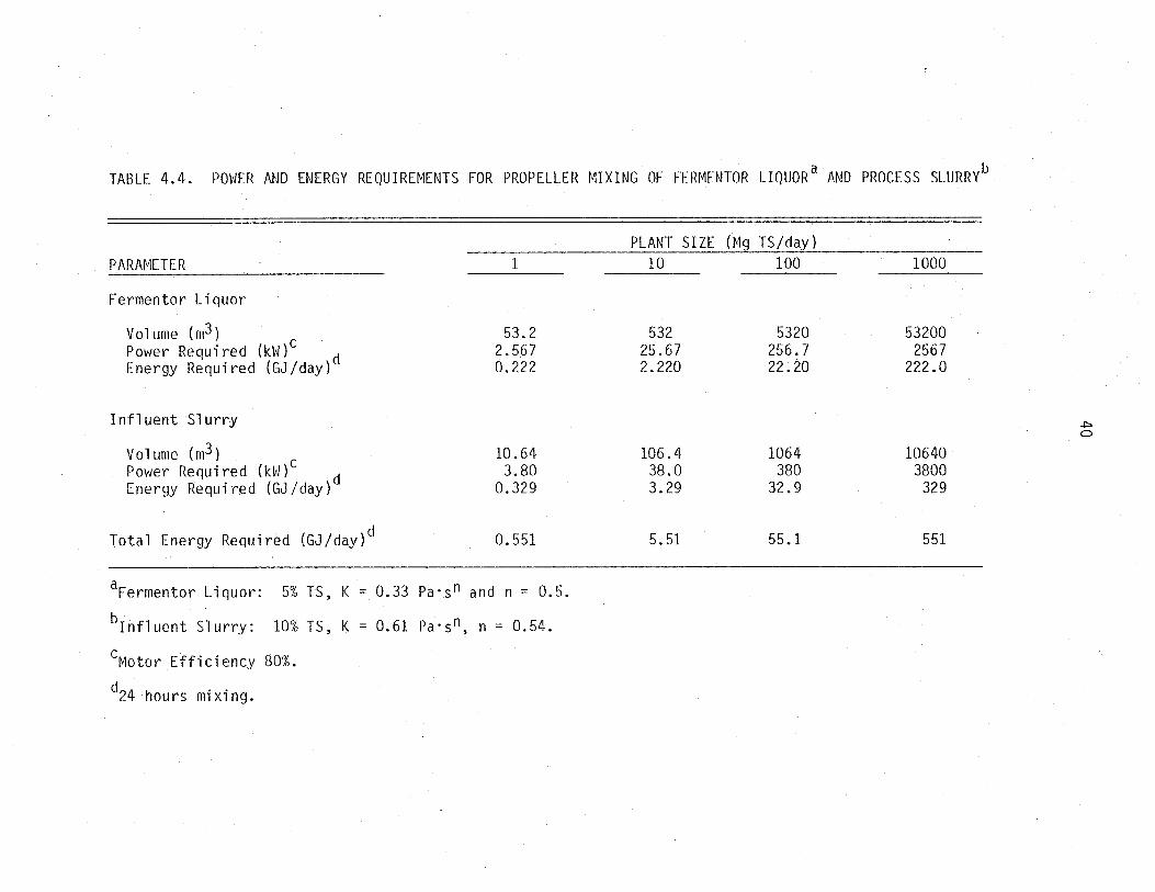
TABLE 4.4. POWER AND ENERGY REQUIREMENTS FOR PROPELLER MIXING OF FERMENTOR LIQUOR a AND PROCESS SLURRyb

PLANT SIZE (~1g TS/day) PARAMETER 1 10 100 1000

Fermentor Liquor

Vo 1 ume (m3) 53.2 532 5320 53200 Power Required (kW)c d 2.567 25.67 256.7 2567 Energy Required (GJ/day) 0.222 2.220 22.20 222.0

Influent Sl urry ~ 0

Vo 1 ume (m3) 10.64 106.4 1064 10640 Power Required (kW)c d 3.80 38.0 380 3800 Energy Required (GJ/day) 0.329 3.29 32.9 329

Total Energy Required {GJ/day)d 0.551 5.51 55.1 551

aFermentor Liquor: 5% TS, K = 0.33 Pa·s n and n = 0.5.

bInfluent Slurry: 10% TS, K = 0.61 P a . 5 n, n = 0.54.

CMotor Efficiency 80%.

d24hours mixing.

TABLE 4.5. SUMMARY OF ENERGY PRODUCTION AND REQUIREMENT FOR ANAEROBIC SYSTEMS FERMENTING BEEF CATTLE MANURE AT 55°Ca

PLANT SIZE (r~g TS / day) PARM1ETER 1 10 100

Gross Methane Energy Production 7.85 78.5 785 (GJ /day)

Heating Energy Requiredb (GJ/day) 3.12 29.79 293.0

Heating Energy Requiredb w/50% 1. 757 16.15 156.5 Effluent Heat Recovery (GJ/day)

Pumping Energy RequiredC (GJ/day) 0.0345 0.283 0.524

Mi xi ng Energy Requiredd (GJ / day) 0.551 5.51 55.1

C02 Scrubbing (GJ / day) 0.2142 2.142 21.42

CH4 Compression (GJ/day) 0.0900 0.900 9.00

aInfluent concentration 80 9 VS/L, HRT = 5 days, Yv = 3.96 013 CH4/m3·fermentor·day.

bAmbient and process slurry temperature, 10°C.

c10 hours of pumping, 300 01 effective length.

d24 hours of mixing.

1000

7850

2907

1543

3.44

551

205

90.0

42

comprises the major portion of the total energy consumption, ranging from 39.7% to 37.0% at an assumed ambient temperature of 10°C. Of this heating energy requirement, 87.4% to 93.9% is used to heat the influent slurry. This indicates the absolute necessity of recovering the effluent heat energy for heating the influent. The heating energy requirement is reduced from 37.0% to 19.7% of the gross energy production for a 1,000 Mg TS/day plant if 50% of the effluent heat is recovered.

The next major energy consumption is mlxlng. It amounts to 7.3% of the total CH4 energy production. Our laboratory and pilot studies showed that the CH4 production did not vary with the duration of daily mixing of the fermentor liquor, indicating that the minimum mixing requirement for fermentation systems may be based on the slurry and effluent handling aspects. The energy consumption of mixing can be cut at· least one half by reducing the mixing time.

The least energy is consumed in pumping. Pumping energy depends less on the plant size because larger pipes can be used for handling larger volumes of the slurry. Energy consumed per volume pumped decreases as pipe size increases. Three hours pumping has higher Reynolds number but requires larger pumps and pipes than 10 hours pumping and therefore involves higher capital cost (Tables 4.2 and 4.3).

The total energy consumption, including C02 scrubbing and CH4 compression, but excluding heating energy, accounts for 11.3% of the gross CH4 energy produc­tion for the 1 Mg TS/day plant and 10.8% for the 1,000 Mg TS/day plant.

4.3.2 Effect of Influent Concentration on Net Thermal Energy Production

Equation 2.1 and Figures 2.2 and 2.3 were used to calculate the gross CH4 production from which the heating requirement was subtracted to determine the net thermal energy production. In calculating the CH4 production at 55°C, m of 0.586 day-1 and K = 0.6, 0.65, 0.8, and 1.3 for So = 60, 70, 80, and 100 g VS/L, respectively, were used. Figure 4.1 shows that at long HRT, higher influent concentration will produce more net thermal energy for the same plant size. However, at HRT less than 12 days, the net thermal energy production increases with So only if So is less than 80 g VS/L. As So increases to 100 g VS/L, the net thermal energy production has a decreases sharply.

4.3.3 Net Thermal Energy Production of tvlesophilic and Thermophilic Systems

Figure 4.2 compares the net thermal energy production from systems fermenting beef cattle manure at mesophilic (35°C) and thermophilic (55°C) temperatures with an influent concentration of 80 g VS/L. At 35°C and So = 80 g VS/L, ~m = 0.326 day-1 and K = 1.7 were used.

Figure 4.2 shows that, at long HRT, mesophilic systems may produce more net thermal energy than thermophil ic systems, but at short HRT, thermophil ic systems wi 11 produce more. The advantage of thermophil i cover mesophil i c systems will increase if the effluent heat is recovered for influent slurry heating.

4. 4 SU~lMARY

This section discussed the energy requirements for anaerobic fermentation

......... ~ 90 0

-0 "'--::> <..9 '--'"

".. 75 -z 0 l-0 ~ 60 -0 0 0::: 0..-

r 45 -(9 n:: w Z W

30 -.J <I: ~ 0::: W I 15 J-

r-W Z 0

0

Figure 4.1.

So = 100 9 V8/L

:= 80 =70 g VS/L

SO= 60 9 VS/L

5 10 15 20 25 HYDRAULIC RETENTION TIME, (days)

Comparing net thermal energy production from thermophilic anaerobic fermentation systems for different influent VS concentration (fermentation temperature 55°C) plant size 10 Mg TS/day, ambient temperature 10°C, and 80 = 0.35 L CH4/g VS).

.j::>. w

-- 100 ~ a

"'0

:::s (9 ..........

.... 80 -z 0 t-O ::J 0 0 60 0:: t'1-

>-<..9 0:: W 40 Z LLI

~ <t ~ et: 20 lLJ I r-1-w a z 0

Figure 4.2.

5 10 15 20 25 HYDRAULIC RETENTION TIME, (days)

Comparing net thermal energy production from mesophilic !35°C) and thermophilic (55°C) anaerobic systems lplant size 10 Mg TS/day, ambient temperature 10 C, So = 80 g VS/L, and 90 = 0.35 L CH4/9 VS. A: 35°C without effluent heat recovery, B: 35°C with 50% heat recovery, C: 55°C without effluent heat recovery, D: 55°C with 50% heat effluent heat recovery).

~ ..J::>

45

systems. The major energy consumption for a thermophilic system is in main­taining the fermentor temperature. Of the total heating energy required, about 89 to 94% was for heating the influent slurry at an ambient temperature of 10°C. The need to recover the heat leaving with the effluent is apparent. With 50% effluent heat recovery, the heating energy requirement is reduced from 37.0% to 19.7% of the gross energy production for a 1,000 Mg TS/day plant.

The next major energy consumption was due to the mlxlng of the influent slurry and fermentor liquor. Mixing amounted to 7.3% of the gross methane energy production, assuming continuous mixing. The mixing energy can be reduced greatly if the mixing time is reduced.

The least energy was consumed in pumping. Pumping energy did not increase when the pumping time was shortened from 10 to 3 hours. Three hours of pumping has a higher Reynolds number but requires a larger pump and bigger pipes.

The total energy consumption excluding thermal energy consumption accounts 10.8 to 11.3% of the gross thermal energy production.

Using the kinetic constants given for different influent concentration and fermentation temperature, it was found that for HRT less than 12 days, the net thermal energy production increased with the influent concentration up to 80 g VS/L and began to drop at influent concentration greater than 80 g VS/L. Also, a longer HRT will produce more net thermal energy at the same influent concentration.

The net thermal energy production for 35° and 55°C were also compared for an influent concentration of 80 g VS/L. This comparison showed that a ther­mophilic (55°C) system will produce more thermal energy than a mesophilic (35°) system unless the fermenter is operated at a very long HRT.

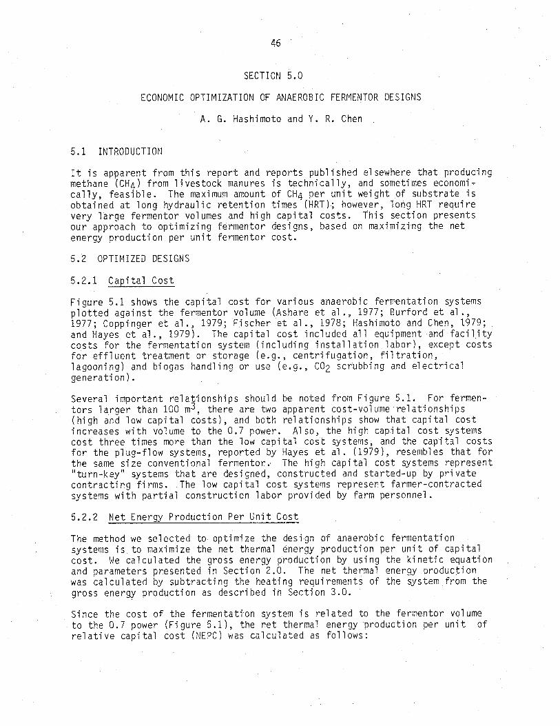
46

SECTION 5.0

ECONOMIC OPTIMIZATION OF ANAEROB IC FERMENTOR DESIGNS

A. G. Hashimoto and Y. R. Chen ,

5.1 INTRODUCTION

It is apparent from this report and reports published elsewhere that producing methane (CH4) from livestock manures is technically, and sometimes economi­cally, feasible. The maximum amount of CH4 per unit weight of substrate is obtained at long hydraulic retention times (HRT); however, long HRT require very large fermentor volumes and high capital costs. This section presents our approach to optimizing fermentor designs, based on maximizing the net energy production per unit fermentor cost.

5.2 OPTIMIZED DESIGNS

5.2.1 Capital Cost

Figure 5.1 shows the capital cost for various anaerobic fermentation systems plotted against the fermentor volume (Ashare et al., 1977; Burford et al., 1977; Coppinger et al., 1979; Fischer 'et al., 1978; Hashimoto and Chen, 1979; and Hayes et al., 1979). The capital cost included all equipment and facil,ity costs for the fermentation system (including installation labor), except costs for effluent treatment or storage (e.g., centrifugation, filtration, lagooning) and biogas handling or use (e.g., C02 scrubbing and electrical generation).

Several important relationships should be noted from Figure 5.1. For fermen­tors larger than 100 m3, there are two apparent cost-volume relationships (high and low capital costs), and both relationships show that capital cost increases with volume to the 0.7 power. Also, the high capital cost systems cost three times more than the low capital cost systems, and the capital costs for the plug-flow systems, reported by Hayes et al. (1979), resembles that for the same si ze conventi onal fermentor. The hi gh capi tal cost systems represent "turn-keyll systems that are desi gned, constructed and started-up by pri vate contracting firms. The low capital cost systems represent farmer-contracted systems with partial construction labor provided by farm personnel.

5.2.2 ~Jet Energy Production Per Unit Cost

The method we selected to optimize the design of anaerobic fermentation systems is to maximize the net thermal energy production per unit of capital cost. vie cal cul ated the gross energy producti on by usi ng the ki neti c equati on and parameters presented in Section 2.0. The net thermal energy production was calculated by subtracting the heating requirements of the system from the gross energy production as described in Section 3.0.

Si nce the cost of the fermentation system is rel ated to the fermentor vol ume ,to the 0.7 power (Figure 5.1), the net thermal energy production per unit of relative capital cost (NEPC) was calculated as follows:

-W-10 6 ...

l-(/) 0 U

-1

~ -J:::>o '-J

0.. <t 105 ()

104~·~~~~~~--~--~~~~--~~~~~--~~~~~~--~~~~~ 10 10 2 103 10

4 10

5 10

6

FERMENTOR VOLUME m3 I t

Fi gure 5.1. Effect of Fermentor Vol ume on Capital Cost (0, Ashare et a 1.. 1977; ., Burford et a 1.. 1977; 0, Coppinger et al., 1979; ", Fischer et al., 1978;!J., Hashimoto et al., 1979; and 0, Hayes et a 1 ., 1979).

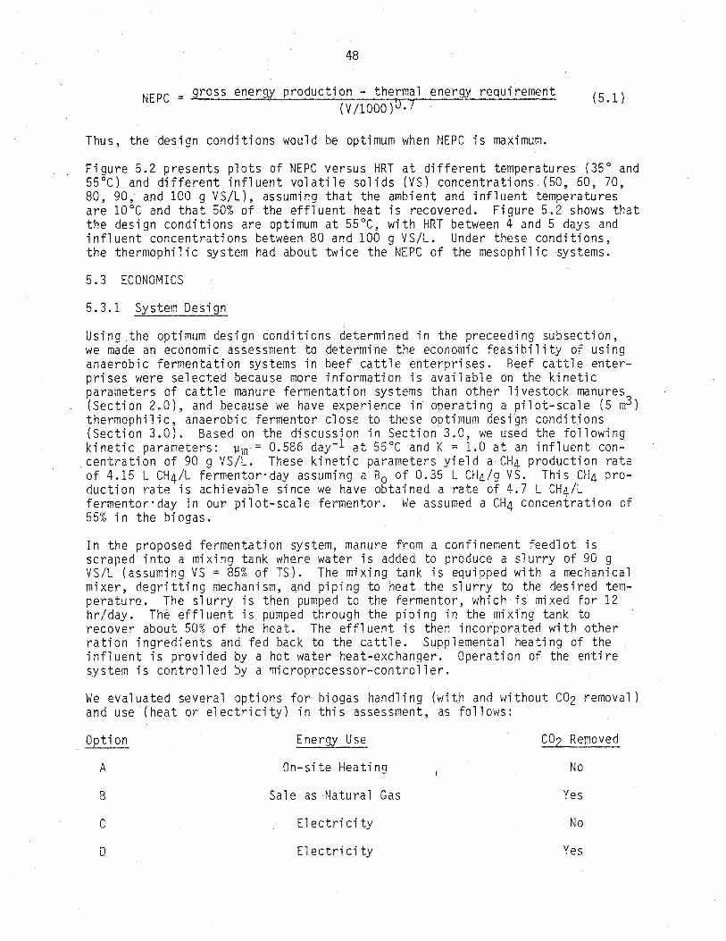
NEPC

48

= gross energy production - thermal energy requirement (V/1000)O.7

Thus, the design conditions \vould be optimum when NEPC is maximum.

(5.1 )

Figure 5.2 presents plots of NEPC versus HRT at different temperatures (35° and 55°C) and different influent volatile solids (VS) concentrations (50, 60, 70, 80, 90, and 100 g VS/l), assuming that the ambient and influent temperatures are 10°C and that 50% of the effluent heat is recovered. Figure 5.2 shows that the design conditions are optimum at 55°C, with HRT between 4 and 5 days and influent concentrations between 80 and 100 g VS/l. Under these conditions, the thermophilic system had about twice the NEPC of the mesophilic systems.

5. 3 ECONO~lICS

5.3.1 System Design

Using the optimum design conditions determined in the preceeding subsection, Y./e made an economi c assessment to determi ne the economic feas i bi 1 i ty of us; ng anaerobic fermentation systems in beef cattle enterprises. Beef cattle enter­prises were selected because more information is available on the kinetic parameters of cattle manure fermentation systems than other livestock manures (Section 2.0), and because we have experience in operating a pilot-scale (5 m3) thermophilic, anaerobic fermentor close to these optimum desi~n conditions (Section 3.0). Based on the discussion in Section 3.0, we used the following kinetic parameters: Pm = 0.586 day-1 at 55°C and K = 1.0 at an influent con­centration of 90 9 VS/l. These kinetic parameters yield a CH4 production rate of 4.15 l CH4/l fermentor'day assuming a 80 of 0.35 l CH4/9 VS. This CH4 pro­duction rate is achievable since we have obtained a rate of 4.7 l CH4/l fermentor'day in our pilot-scale fermentor. We assumed a CH4 concentration of 55% in the biogas.

In the proposed fermentation system, manure from a confinement feedlot is scraped into a mi xi ng tank where water is added to produce a sl urry of 90 g VS/l (assuming VS = 85% of TS). The mixing tank is equipped with a mechanical mixer, degritting mechanism, qnd piping to heat the slurry to the desired tem­perature. The slurry is then pumped to the fermentor, which is mixed for 12 hr/day. The effluent is pumped through the piping in the mixing tank to recover about 50% of the heat. The effluent is then incorporated with other ration ingredients and fed back to the cattle. Supplemental heating of the i nfl uent is provi ded by a hot y./ater heat-exchanger. Operati on of the enti re system is controlled by a microprocessor-controller.

We evaluated several options for biogas handling (with and without C02 removal) and use (heat or electricity) in this assessment, as follows:

Option Energy Use CO2 Removed

A On-site Heating No

B Sale as Natural Gas Yes

C El ectri city No

0 El ectri ci ty Yes

l'f) E '-. J 120 (9

.... 1- 55 Q C U) 0 90 g VS/L 0 100 -

l-Z ~

0:: 80

liJ 0-

Z 0 60 - 60 g VSI -~-0 35°C :) 80 g VS/L 0 -0 40 Ct: 0..

>-(9 G:: 20 w Z W

I- 0 W Z 0 2 4 6 8 10

HYDRAULIC RETENTION TIME, days

Figure 5.2. Effect of Hydraulic Retention Time, Temperature and Influent Concentration on the Net Energy Production Per Unit Cost.

..p. 1.0

50

For all of these options, H2S and moisture are removed from the biogas by the iron sponge and glycol absorption processes, and the gas is compressed and stored at 860 kPa in tanks with a l-day gas-production capacity. These pro­cesses are necessary to prevent corrosion and to allow some flexibility to modulate the variation in daily gas production. The C02 is removed by the water-stripping pro~ess.

Table 5.1 summarizes the fermentor volume, energy requirements, and net energy production for the various options and plant sizes. Procedures used to calcu-1 ate the vol ume and number of fermentors and energy requi rements are presented in Section 4.0.

Since the efficiency of an internal combustion engine to convert CH4 into use­ful work increases as the engine size increases, the engine-generator effi­ciency 'v-/as estimated by the following equation (assuming a 95% efficient generator and engine efficiencies published by Evans et al., 1973):

Engine-generator efficiency (%) = 4.18 1n (E) + 11.61 (5.2)

where E is the gross energy input to the engine (GJ/day) and the maximum effi­ciency is 38%. Equation 5.2 i~ only applicable for engines fueled with 100% CH4; therefore, Equation 5.2 is applicable only for Option D. The engine­generator efficiencies for Option C were assumed to be 60% of that calculated from Equation 5.2, since the useful work output per unit energy input of a high compression engine, receiving gas containing 55% CH4, is 60% of an engine receiving 100% CH4 (Neyeloff and Gunkel, 1975).

The net CH4 production, shown in Table 5.1, was calculated by subtracting the net heating requirement from the gross energy production. The net electrical production was calculated by subtracting the electrical energy requirements from the electrical energy produced by the engine-generator. Option 0 pro­duced more net electrical energy than Option C because the higher engine­generator efficiency of Option 0 was sufficient to offset the increased energy for C02 removal.

We assumed that the waste heat from the engine would be used to heat the fermentor. This assumption is justified since the net heating requirement is only about 20% of the total energy production, and between 20 to 30% of the gross energy consumed by the engine can be recovered from the jacket cooling system. Since an additional 26 to 30% of the heat can be recovered from the engine exhaust, Options C and 0 can be a source of low temperature (75 to 85°C) process It/ater, as well as electricity. We did not assume any use of the excess waste heat from the engine generator in our energy balance, nor did we assess any credit for the excess heat generated.

5.3.2 Capital Cost

Table 5.2 shows the installed equipment costs for major components of a 1860 m3 anaerobi c fermentati on system, usi ng the vari ous bi ogas handl i ng and use options identified above. The costs shown in Table 5.2 were used as the basis to estimate the total capital cost at various plant sizes. Total capital costs were estimated by using engineering and inspection fees, contingency, escalation and start-up costs of 14, 10, 18 and 10% of installed equipment costs, respectively. To estimate the total capital costs for different plant sizes, the scale-up factor of digester volume to the 0.7 power, as shown in

51

TABLE 5.1. ENERGY PRODUCTION AND REQUIREMENTS a FOR VARIOUS PLANT SIZES AND ENERGY USE OPTIONS

PLANT SIZE, Mg TS/day

PARAiv1ETER 1 10

Working volume, m3 47 472

Gross energy producti on, MJ /day 7,300 73,000

Energy requirements, MJ/day Net heating 1,550 14,100 Mixing 143 1;430 Pumping 21 129 Gas compression 152 1,520 Scrubbing pump 111 1,110

Electrical generator efficiency, % Option C 12 18 Option D 20 30

Net CH4 productionb, MJ/day Options A & B 5,750 58,900

Net el ectri ca 1 producti an b, t~J / day Option C 574 10,100 Option D 1,030 17,400

100

4,720

730,000

136,000 14,300

635 15,200 11 , 100

24 38

594,000

145,000 236,000

aAssumes 50% effluent heat recovery, 12 hr/day mixing of influent and fermentor, 10 hr/day pumping of influent and effluent, and ambient and influent tem­perature of 10°C.

bGross production minus requirement (thermal or electrical energy).

52

TABLE 5.2. INSTALLED EOUIPfY1ENT COSTS FOR ~1AJOR COMPONENTS OF A 1860 m3 ANAEROBIC FERMENTOR

COST (i n $1000 )

CO~lPONENT A B C

Premix & degrit 50 50 50

Pump 30 30 30

Fermentor w/mixer 250 250 250

Heat exchanger 20 20 20

Piping 10 10 10

Microprocessor-controller 20 20 20

Gas cleaner 50 50 50

CO2 scrubber 200

Compressors & storage tanks 100 50 100

Boiler 30 30

Engine-generator w/heat exchangers 100

TOTAL INSTALLED EQUIPMENT COST 560 710 630

D

50

30

250

20

10

20

50

200

50

100

780

53

TABLE 5.3. COSTS FOR PRODUCING METHMJE AND ELECTRICITY AT VARIOUS PLANT SIZES

PLANT SIZE, Mg TS/day

PARM1ETER 1 10 100

Capital costs, $1000 Option A 65 327 1,640 Option B 83 417 2,090 Option C 73 365 1,830 Option D 91 454 2,270

Labor costs, $1000/yr 11 22 43

Fixed costs, $1000/yr Opti on A 16 79 394 Option B 20 100 501 Option C 17 87 439 Option D 22 109 546

Uti 1 ity costs, $1000/yr Option A 1.7 17 164 Option B 2.2 22 220 Option C 0.1 1 11 Option D 0.1 1 11

Total annual costs, $1000/yr Option A 29 117 600 Option Ala 10 48 306

Option B 34 144 764 Option Bla 12 62 398

Option C 29 111 492 Option Cia 9 36 168

Option D 33 132 600 Option D'a 10 43 204

aLow cost option assumes labor and fixed costs to be 25% and 33%, respectively, of high cost option.

54

Figure 5.1, was used. Table 5.3 shows the total capital costs for the various options and plant sizes.

5.3.3 Annual Costs

Annual costs (labor, fixed and utility costs) were estimated fo~ the various plant sizes (Table 5.3). Salaries for the plant operators were assumed to range from $ll,OOO/yr for the 1 Mg TS/day plant up to $43,OOO/yr for the 100 Mg TS/day plant.

Fixed costs were calculated assuming an interest rate of 14% and a 20-year straight-line depreciation of the total capital cost. Taxes, insurance, and repair and maintenance were estimated to be 3, 1.5 and 3% of the installed equipment cost, respectively.

Utility costs were calculated based upon the energy requirements in excess of that produced. Utility rates were assumed to be $14/GJ (5\1/kv/h) for electri­city and $0.11/m3 for make-up water. The utility costs shown for Options A and 8 reflect electricity and water charges. The only utility cost charged to Opt; cins C and 0 was for make-up water, si nee the engi ne-generator produced more el ectri city and waste heat than needed by the fermentati on system.

Table 5.3 also shows the total annual costs for the low cost, farmer­contracted and operated systems. The capital costs for these systems were assumed to be one-third the cost of a comparably sized, "turn-key" plant (Figure 5.1). The labor costs were assumed to be one-quarter of the high cost system. This low level of labor can be justified because of the use of microprocessor-controllers to operate and monitor much of the routine operation.

5.3.4 Energy Production Costs

Energy production costs were calculated by dividing the total annual cost for each opti on by the annual net energy (CH4 or el ectri city) produced by each option. The effect of plant size on CH4 production costs for the high cost systems (Options A and 8) and the low-cost systems (Options AI and 8 1

) are shown in Figure 5.3. The plant size at which CH4 production costs equal the current natural gas prices of $3/GJ would be 75, greater than 300, 4.2 and 6.7 Mg TS/day for Options A, 8, AI and 8 1

, respectively. Thus, although there is only about a three-fold difference in total annual cost between Option A and AI, there is about an 18-fold difference in break-even plant size.

Fi gure 5.4 shows the effect of plant si ze on el ectri ci ty producti on costs. The plant sizes at which the electricity production costs equal the current electricity rate of $14/GJ (5\1/kWh) would be 43, 22, 5.3 and 2.8 Mg TS/day for Options C, 0, CI and 0 1

, respectively. These results show that there is an eight-fold difference in break-even plant size between the low-cost and high­cost systems, and that the increased electricity generation efficiency, caused by scrubbing C02 from the biogas (Options 0 and 0 1

), more than compensates for the increased total annual costs.

Table 5.4 lists the energy production costs for the various options at dif­ferent plant sizes (1, 10 and 100 Mg TS/day) and an effluent feed credit of S60/Mg effluent TS. The production costs with effluent feed credit were calculated by subtracting the feed credit from the total annual cost and by

J

~ -tIT

12 r: (/) 0 u

z 0 I- 8 <-) ::> a 0 0:: ll.

LlJ B Z 4 « A I i-lLl 8' ~

A

20 40 60 80 100 PLANT SIZE, Mg TS/day

Figure 5.3. Effect of Plant Size on Methane Production Costs (Temperature = 55°C, HRT = 5 days, So = 90 9 VS/L. A = High Cost, no C02 Removal; n = High Cost, C02 removal; A' = Low Cost, no C02 Removal; 8' = Low Cost, C02 Removal).

01 01

140

J 120 (9

"'-4:A-

... t- 100 (I) 0 0

Z 0 80 1-() :J 0 0 60 . cr: (L

>-t- 40 .. 0 cr: ~ 0 w 20--.J W

20 40

PLANT SIZE, Mg

J

60

TS/day 80 100

Figure 5.4. Effect of Plant Size on Electricity Production Cost (Temperature = 55°C, HRT = 5 days, So = 90 9 VS/L. C = High Cost, no C02 Removal; 0 = High Cost, C02 Removal; C' = Low Cost, no C02 Removal; 0 1 = Low Cost, C02 Removal).

CJ1 0"1

57

TABLE 5.4. ENERGY PRODUCTION COSTS a FOR VARIOUS PLANT SIZES, ENERGY PRODUCTION OPTIONS AND EFFLUENT FEED CREDITS

PLANT SIZE, Mg TS/day 1 10 100

Feed Credit Feed Credit Feed Credit

OPTION $O/Mg $60/Mg $0 /~1g $60/Mg $O/Mg $60 /~~g

A 13.71 8.01 5.46 -0.11 2.77 -2.76 AI 4.67 -1.04 2.26 -3.32 1.41 -4.11

B 15.88 10.23 6.67 1.14 3.49 -1.99 BI 5.57 -0.09 2.83 -2.70 1.82 -3.66

C 138.36 81.18 29.98 -2.46 9.31 -13,35 CI 41.87 -15.31 9.68 -22.76 3.17 -19.49

0 88.68 56.74 20.83 1. 94 6.96 -6.94 0 1 27.19 -4.75 6.76 -12.13 2.36 -11. 54

aCosts expressed as $/GJ.

58

dividing the difference by the annual net energy production. The results in Table 5.4 indicate that the break-even plant sizes are decreased to between 3 and 8 Mg TS/day for the high cost systems when the effluent feed credit is used. For the low cost systems, the break-even plant size is less than 1 ~~g TS/day when the effluent feed credit ;s used.

5.3.5 Implications of this Assessment

This economic assessment has shown that CH4 can be economically generated at moderate plant sizes (3 to 6 Mg TS/day) when farmer-constructed and operated systems are used or when "turn-key" systems use an effl uent feed credit of $60/~1g effluent TS. Assuming that 2.8 kg TS/day can be recovered from a con­fined steer, the break-even plant size discussed above would serve feedlots between 1,000 to 2,000 cattle. If the farmer-constructed and operated systems also fed the fermentor effluent, then anaerobic fermentation systems would be economically feasible for feedlots of less than 300 cattle.

In this assessment, we assumed that all of the energy produced would be used. Lipper et al. (1976) reported that the energy requirements for energy-intensive commercial feedlots in Kansas were 2.2 GJ/head'yr for natural gas and 0.32 GJ/head'yr for electricity. The net energy production from a plant receiving manure from a 1,000-head feedlot would be about 6.2 GJ/head'yr of CH4 (Options A and B) or 0.9 (Option C) and 1.6 GJ/head"yr (Option D) of electricity. Thus, more energy would be produced by these systems than could be used by the livestock enterprise. Strategies must be developed to utilize this excess energy. Conscientious effort must be exercised to adjust energy use to pro­ducti on at the enterpri se level, and there must be the opportuni ty to sell the surplus energy.

5. 4 SU~1MAR Y

We have presented our approach to optimizing anaerobic fermenter designs by selecting design criteria that maximize the net energy production per unit cost. Using this optimization technique, we estimate that a farmer-constructed and operated system would be economically feasible for beef feedlots between 1,000 to 2,000 head without an effluent feed credit, and about 300 head with an effl uent feed credi t of $60/~1g eff1 uent TS. Commerci a 1 "tu rn-key" systems are only feasible for feedlots larger than 8,000 head when an effluent credit is not used, and for feedlots between 1,000 to 2,000 head when an effluent feed credit of $60/Mg effluent TS is used. Based on these results, we believe that the economics of anaerobic fermentation is sufficiently favorable for farm-scale application of this technology.

59

SECTION 6.0

ACKNOWLEDGEMENTS

The authors wish to acknowledge the technical support provided by Robin Anderson, Lorrin Barth, Jim Chapman, Misi Eich, Susie Hassler, Gary Klein, Brad McConnell, Lynn Niemann, Mike Overturf, Steve Robinson, Larry Roehl and Moira Wilhelm.

60

SECTION 7.0

REFERENCES

1. American Public Health Association. 1975. Standard Methods for the Examination of \~ater and Wastewater, 14th ed., Amer. Pub. Health Assoc., Inc., New York.

2. Andrews, J. F. and E. A. Pearson. 1965. Kinetics and characteristics of volatile acid production in anaerobic fermentation processes. International Journal Air Water Pollution 9:439.

3. Ashare, E., D. L. Wise, and R. L. Wentworth. 1977. Fuel gas production from animal residue. Engineering Report, Dynatech RID Company. Dynatech Report No. 1551. Cambri dge, r~A.

4. Ashare, E., D. C. Augenstein, D. C. Young, R. J. Hassan, and G. L. Duret. 1978. Evaluation of systems for purification of fuel gas from anaerobic di gesti on. Eng; neeri ng Report, Dyna tech RID Company. Dynatech Report No. 1628. Cambri dge, ~1A.

5. Augenstein, D. C., D. L. Wise, and C. L. Cooney. 1976. Biomethanation: Anaerobic fermentation of C02/H2 and CO to methane. Presented at the 69th Annual Meeting of the AICHE, November 28 to December 2, 1976w Chicago, IL.

6. Bates, R. L., P. L. Fondy, and J. G. Fenic. 1966. Impeller charac­teristics and power, in Mixing (I), V. W. Uhl and J. B. Gray, Eds., -Academic Press, NY.

7. Bryant, M. P. 1974. Nutritional features and ecology of predominant anaerobic bacteria of the intestinal tract. Amer. J. Clin. Nutr. 27:1313.

8. Bryant, M. P. 1976. The microbiology of anaerobic degradation and metha-nogenesis with special reference to sewage. p. 107. In: H. G. Schlegel (ed.). Symposium on r~icrobial Energy Conversion. E. Goltze KG, Gottingen, Germany.

9. Bryant, M. P. 1979. Microbial methane production-theoretical aspects. J. Anim. Sci. 48:193.

10. Bryant, r~. P., S. F. Tzeng, 1. M. Robinson and A. E. Joyner Jr. 1971. Nutrient requirements of methanogenic bacteria. p. 23. In: R. F. Gould (ed.). Anaerobic Biological Treatment Processes, Advances in Chemistry, Series 105. Amer. Chern. Soc., Washington, D.C.

11. Bryant, M. P., V. H. Yarel, R. A. Frobish and H. R. Isaacson. 1976. Biological potential of thermophilic methanogenesis from cattle wastes. In: H. G. Schlegel (ed.). Seminar on ~1icrobial Energy Conversion. E. Goltze KG, Gottingen, Germany.

12. Bryant, ~1. P., L. L. Campbell, C. A. Reddy and ri. R. Crabill. 1977. Growth of desulfovibrio in lactate or ethanol media low in sulfate in asso­ciation with H2-utilizing methangenic bacteria. Appl. Environ. r1icrobiol. 33:1162.

61

·13. Buhr, H. O. and J. F. Andrews. 1977. The thermophilic anaerobic digestion process. Water Res. 11:129.

14. Burford, J. L., F. T. Varani, S. Schellenbach, W. F. Shelley and B. Pace. 1977. Energy potential through bio-conversion of agricultural wastes: Phase II. Final Report to Four Corners Regional Commission, Grant No. 672-366-002. Bio-Gas of Colorado, Inc., Arvada, CO.

15. Chen, M. and M. J. Wolin. 1979. Effect of monensin and lasalocid-sodium on the growth of methanogenic and rumen saccharolytic bacteria. Applied and Environmental t~icrobiology 38:72-77.

16. Chen, Y. R., and A. G. Hashimoto. 1976. Pipeline transport of livestock waste slurries. The TRANSACTIONS of the ASAE. 19:(5):898-902,906.

17. Chen, Y. R. and A. G. Hashimoto. 1978. Kinetics of methane fermentation. p. 269. In: C. D. Scott (ed.). Proc Symp. on Biotechnology in Energy Production and Conservation. John Wiley, New York.

18. Chen, Y. R., and A. G. Hashimoto. 1979. Impeller mixing power require­ment. Presented at the 1979 Winter meeting of the ASAE. New Orleans, LA. ASAE Paper No. 79-4583, St. Joseph, MI.

19. Chiu, S. Y., L. T. Fan, I. C. Kao and L. E. Erickson. 1972a. Kinetic behavior of mixed populations of activated sludge. Biotechnol. and 8ioeng. 14:179.

20. Chiu, S. Y., L. E. Erickson, L. T. Fan and I. C. Kao. 1972b. Kinetic model identification in mixed populations using continuous culture data. Biotechnol. and Bioeng. 14:207.

21. Contois, D. E. 1959. Kinetics of bacterial grov/th: relationship between population density and specific growth rate of continuous cultures. J. Gen. t~icrobiol. 21:40.

22. Converse, J. C., G. W. Evans, C. R. Verhoven, W. Gibbo~, and M. Gibbon. 1977a. -Performance of a large size anaerobic digester for poultry manure. Paper No. 77-0451, ASAE, St. Joseph, Michigan.

23. Converse, J. C., J. G. Zeikus, R. E. Graves and G. W. Evans. 1977b.

24.

Anaerobic degradation of dairy manure under mesophilic and thermophilic temperatures. TRANSACTIONS of the ASAE 20:336.

Cooney, C. L. an~ D. L. Wise. 1975. solid waste for fuel gas production.

Thermophilic anaerobic digestion of Biotechnol. Bioeng. 17: 1119.

25. Coppinger, E., J. Brautigam, J. Lenart and D. Baylon. 1979. Report on the design and operation of a full-scale anaerobic dairy manure digester. Final Report to the U.S. Department of Energy, EG-77-C-06-1016. Solar Energy Research Institute, Golden, CO. 84 p.

26. Eckenfelder, W. W., Jr. 1963. Mathematical formulation of the biological oxidation process. p.277. In: W. Yl. Eckenfelder and J. t-1cCabe(eds.). Advances in Biological Waste Treatment. Permagon Press, New York.

62

27. Eli Lilly. 1975. Rumensin Technical Manual. Indianapolis, Indiana.

28. Evans, Jr., F. L., C. R. Olson, H. Steen-Johnson, V. H. Abadie Jenett. 1973. Process machinery drives. p. 24.1-24.50. In: Perry and C. H. Chilton (Eds.). Chemical Engineers Handbook. McGraw-Hill Book Co., New York.

and E. R. H.

29. Fischer, J. R., D. M. Sievers and C. D. Fulhage. 1975. Anaerobic digestion in swine wastes. p.307. In: \~. J. Jewell (ed.). Energy, Agriculture and \~aste ~1anagement. Ann Arbor Science, Ann Arbor, ~~ichigan.

30. Fischer, J. R., D. ~~. Sievers and E. L. Iannotti. 1978a. Biological and chemical fluctuations during anaerobic digestion of swine manure. ASAE Paper 78-4011, ASAE, St. Joseph, Michigan.

31. Fischer, J. R., E. L. Iannotti, D. M. Sievers, C. D. Fu1hage and N. F. Meador. 1978b. ~lethane production systems for swine manure. p. 45-76. In: J. M. Sweeten (Ed.). Proc. Great Plains Sem. on Methane Production from Livestock Manure. College Station, TX.

32. Fi scher, J. R., E. L. Iannotti, J. H. Porter and A. Garci a. 1979. Producing methane gas from swine manure in a pilot-size digester. Trans. Am. Soc. Agr. Engr. 22:370.

33. Garrett, ~1. T., Jr. and C. N. Sawyer. 1952. Kinetics of removal of soluble BOD by activated sludge. p. 51. In: Proceedings, 7th Industrial Waste Conference,Purdue University, Lafayette, Indiana.

34. Go1ueke, C. G. sewage sludge.

1958. Temperature effects on anaerobic digestion of raw Sewage and Industrial Wastes 30:1225.

35. Grady, C. P. L., Jr., L. F. Harlow and R. R. Riesing. 1972. Effects of growth rate and influent substrate concentration on effluent quality from chemostats containing bacteria in pure and mixed culture. Biotech. and Bioeng. 14:391.

36. Grau, P., M. Dohanyos andfJ. Chudoba. 1975. Kinetics of multicomponent substrate concentrate removal by acti vated sl udge. Hater Research 9: 637.

37. Hashimoto, A. G. and Y. R. Chen. 1979. Anaerobic fermentation of beef cattle and crop residues. Proceedings, Third Annual Fuels from Biomass Symposium, June 4-6, Golden, CO, 491.

38. Hashimoto, A. G., V. H. Vare1 and Y. R. Chen. 1979b. Factors affecting methane yield and production rate. ASAE Paper No. 79-4583. ASAE, St. Joseph, Michigan.

39. Hashimoto, A. G., Y. R. Chen, and V. H. Varel. 1980. Theoretical aspects of methane production: State-of-the-Art. Presented at the Fourth International Symposium on Livestock ~lastes; Amarillo, TX, April 15-17, 1980.

40. Hayes, T. D., W. J. and D. F. Sherman. First International Cardiff, Wales.

Jewell, A. Dell'Orto, K. J. Fanfoni, A. P. Leuschner 1979. Anaerobic digestion of cattle manure. Handout, Symposium on Anaerobic Digestion. University College,

63

41. Hill, D. T. and C. L. Barth. 1977. A dynamic model for simulation of animal waste digestion. J. Wat. Pol. Cont. Fed. 49:2129.

42. Hills, D. J. 1979. Effects of carbon:nitrogen ratio on anaerobic digestion of dairy manure. Agricultural ItJastes 1:(4):267-278.

43. Hobson, P. N., S. Bousfield and R. Summers. 1974. Anaerobic digestion of organic matter. p. 131. In: Critical Reviews in Environmental Control, Chemical Rubber Co., Cleveland.

44. Hungate, R. E. 1966. In: The Rumen and Its Microbes, Academic Press, New York.

45. Jewell, ltJ. J., H. R. Davis, H. H. Gunkel, D. J. Lathwell, J. H. Martin, Jr., T. R. ~'1cCarty, G. R. Morris, D. R. Price and D. i~. Hilliams. 1976. Bioconversion of agricultural wastes for pollution control and energy conservation. Final Report, ERDA-NSF-741222A01. Cornell University, Ithaca, New York.

46. Johnstone, R. E., and M. W. Thring. 1957. scale-up methods in chemical engineering.

Pilot plants, models, and McGraw-Hill Book Co., NY.

47. Kaspar, H. F. and K. Wuhrman. 1978. Kinetic parameters and relative turnovers of some important catabolic reactions in digesting sludge. Appl. Environ. ~1icrobiol. 36:1.

48. Kirsch, E. J. and R. t~. Sykes. 1971. Anaerobic digestion in biological waste treatment. p.155. In: D. J. D. Hockenhull and J. and A. Churchill (eds.). Progress in Industrial Microbiology. London.

49. Kroeker, E. J., H. M. Lapp, D. D. Shculte and A. 8. Sparling. 1975. Cold weather energy recovery from anaerobic digestion of swine manure. p. 337-352. In: \oj. J. Jewell (ed.). Energy, Agriculture and ~~aste t1anagement. Ann Arbor Science, Ann Arbor, MI.

50. Kroeker, E. J., D. D. Schulte, A. B. Sparling and H. M. Lapp. 1979. Anaerobic treatment process stability. J. Itlater Poll. Control Fed. 51:718.

51. Kugelman, I. J. and P. L. t/1cCarty. 1965. Cation toxicity and stimulation in anaerobic waste treatment. J. Water Pollut. Control Fed. 37:97.

52. Lapp, H. ~1., D. D. Schulte, E. J. Kroeker, A. B. Sparling and B. H. Topnik. 1975. Start-up of pilot scale swine manure digesters for methane production. p. 234. In: Proc. 3rd Int. Symp. Livestock Wastes. Amer. Soc. Agr. Eng., St. Joseph, Michigan.

53. Lawrence, A. W. and P. L. McCarty. 1969. Kinetics of methane fermen­tation in anaerobic treatment. Journal Hater Pollution Control Federation 41:Rl.

54. Lipper, R. 1., J. A. Anschutz and J. C. Walker. 1976. Energy require­ments for commercial beef feedlots in Kansas. Summary Report to the Kansas State Department of Health, Division of Environment Health Services, Kansas State University, ~'1anhattan, KS.

64

55. ~~ah, R. A., D. M. Ward, L. Bareski and T. L. Glass. 1977. Biogenesis of methane. Ann. Rev. Microbial. 31:309.

56. McCarty, P. L. 1964a. Anaerobic waste treatment fundamentals, II. Environmental requirements and control. Public Works 95:123.

57. McCarty, P. L. 1964b. Anaerobic waste treatment fundamentals, III. Toxic materials and their control. Public Works 95:91.

58. ~~cCarty, P. L. 1964c. The methane fermentation. p. 314. In: H. Henkelekian and N. C. Dondero (eds.). Principles and Applications in Aquatic Microbiology. John Wiley and Sons, Inc., New York.

59. McCarty, P. L. and R. E. ~~cKinney. 1961. Volatile acid toxicity in anaerobic digestion. J. Water Pollut. Control Fed. 33:223.

60. ~1cInerney, M. J. and M. P. Bryant. 1978. Syntrophic association of H2-utilizing methanogenic bacteria and H2-producing alcohol and fatty acid­degrading bacteria in anaerobic degradation of organic matter. In: Proceedings of the Symposia, Anaerobiosis and Anaerobic Infection. Gustav-Fischer, Verlag Stuttgart, Germany.

61. McKinney, R. E. 1962. Mathematics of complete mixing activated sludge. Journal Sanitary Engineering Division, Am. Soc. of Civil Eng. 88:87.

62. fvlonod, J. 1950. The techni que of conti nuous culture theory and app 1 i ca­tions. Annales de l'Institut Pasteur 79:390.

63. Morris, G. R. 1976. Anaerobic fermentation of animal wastes: a kinetic and empirical design evaluation. M.S. Thesis, Cornell University, Ithaca, New York.

64. Mountfort, D. O. and R. A. Asher. 1978. Changes in proportions of ace­tate and carbon dioxide used as methane precursors during the anaerobic digestion of bovine waste. Appl. Environ. Microbiol. 36:648.

65. Neyeloff, S. and W. W. Gunkel. 1975. Methane-carbon dioxide mixtures in an internal combustion engine. p. 397-408. In: H. J. Jewell (Ed.). Energy, Agriculture and Haste Management. Ann Arbor Science, Ann Arbor, MI.

66. O'Rourke, J. R. 1968. Kinetics of anaerobic treatment at reduced tem­peratures. Ph.D. Thesis, Stanford University, S~af'J-ford, California.

67. Perry, R. H. and C. H. Chilton. 1973. Chemical Engineers ' Handbook.

68.

Fifth Edition. McGraw-Hill Book Co., New York.

Pfeffer, J. T. 1974. Temperature effects on anaerobic fermentation of domestic refuse. Biotechnol. Bioeng. 16:771-787.

69. Pfeffer, J. T. and J. C. Liebman. 1976. Energy from refuse by bioconver­sion, fermentation and residue disposal process. Resource Recov. Conserv. 1: 3.

70. Pi rt, S. J. reclamation.

1978. Aerobic and anaerobic microbial digestion in waste J. Applied Chemical Biotechnology, 28, 232.

65

71. Scheifinger, C. C. and M. J. Wolin. 1973. Propionate formation from cellulose and soluble sugars by combined cultures of Bacteroides suc­cinogenes and Selenomonas ruminantium. Appl. Microbiol. 26:789. ---

72. Sievers, D. ~1. and D. E. Brune. 1978. Carbon/nitrogen ratio an9 anaero­bic digestion of swine waste. Trans. Am. Soc. Agr. Engr. 21:537.

73. Smith, P. H. and R. A. Mah. 1966. Kinetics of acetate metabolism during sludge digestion. Appl. Microbiol. 14:368.

74. Speece, R. E. and P. L. McCarty. biological solids accumulation in International Conference on Water New York.

1964. Nutrient requirements and anaerobic digestion. p. 305. In: Pollution Research. Permagon Press,

75. Stevens, M. A. and O. O. Schulte. 1979. Low temperature anaerobic digestion of swine manure. J. Env. Engr. Div., ASCE 105:33.

76. Summers, R. and S. Bousfield. 1980. A detailed study of piggery-waste anaerobic digestion. Agricultural Wastes 2:61-78.

77. Torien, D. F. and W. H. J. Hattingh. 1969. Anaerobic digestion, 1. The microbiology of anaerobic digestion. Water Res. 3:385.

78. Turnocliff, W. and M. Custer. design for a hog farm. Final Energy Conservation, Contract Colorado.

1978. Evaluation of methane gas system and report to the state of Colorado, Office of No. OEC-00003. Bio-Gas of Colorado, Arvada,

79. Varel, V. H., H. R. Isaacson and ~~. P. Bryant. 1977. Thermophilic methane production from cattle waste. Appl. Environ. Microbiol. 33:298.

80. Varel, V. H., A. G. Hashimoto and Y. R. Chen. 1980. Effect of tem­perature and retention time on methane production from beef cattle manure. Appl. Environ. Microbiol. 40:(2):217.

81. Varel, V. H. and A. G. Hashimoto. 1981. Effect of monensin and chlor­tetracycline on methane production from beef cattle wastes. Appl. Environ. ~1icrobiol. 41: (1) :xxx- (accepted).

82. Wael, L. L., Sr., and C. W. Gehrke. 1975. An automated total protein nitrogen method. Journal of the AOAC. 48: (6):1221.

83. Winfrey, M. R. and J. G. Zeikus. 1977. Effect of sulfate on carbon and electron flow during microbial methanogenesis in freshwater sediments. Appl. Environ. Microbiol. 33:275.

84. \~infrey, ~1. R., D. R. Nelson, S. C. Klevickis and J. G. Zeikus. 1977. Association of hydrogen metabolism vlith methanogenesis in lake Mendota sediments. Appl. Environ. Microbiol. 33:312.

85. ~Iolfe, R. S. 1971. Microbial formation of methane. p. 107. In: A. W. Rose and A. \~. Hilkinson (eds.). Advances in ~'1icrobial Physiology. Academic Press, New York.

86.

66

Wolfe, R. S. 1979. ~1icrobial biochemistry of methane - a study in contrasts. p.293. In: J. R. Quayle (ed.). Microbial Biochemistry. Volume 21. University Park Press, Baltimore.

87. Wolin, M. J. 1974. Metabolic interactions among intestinal microorga­nisms. Amer. J. Clin. Nutr. 27:1320.

88. Wolin, M. J. 1976. Interaction between~H2 producing and methane­producing species. p. 141. In: H. G. Schlegel, G. Gottschalk and N. Pfenning (eds.). Microbial Formation and Utilization of Gases (H2' CH4, C02)' Goltze KG, Gottingen, Germany.

89. Zeikus, J. G. 1977. Biology of methanogenic bacteria. Bacteriol. Rev. 41:514.

90. Zeikus, J. G. 1979. Microbial populations in anaerobic digesters. First International 'Symposium on Anaerobic Digestion, University Industry Center, University College, September 17-21, Cardiff, Wales.

Document Control 11. SERI Report No. Page TR~98372-l

NTIS Accession No. 3. Recipient's Accession No.

4. Title and Subtitle 5. Publication Date

Anaerobic Fermentation of Beef Cattle Manure January 1981 6.

7. Author(s) 8. Performing Organization Rept. No. A.G. Hashimoto. Y.R. Chen V.H. Varel

9. Performing Organization Name and Address Roman L. Hruska U.S. Meat Animal Research Center U.S. Department of Agriculture Clay Center, Nebraska

12. Sponsoring Organization Name and Address Solar Energy Research Institute 1617 Cole Boulevard Golden, Colorado 80401

15. Supplementary Notes

SERI Technical Honitor: Dan Jantzen

10. Project/Task/Work Unit No. 3335.01

11. Contract (C) or Grant (G) No.

(C) DB-9-8372-l

(G)

13. Type of Report & Period Covered

Technical Report 14.

16. Abstract (Limit: 200 words) This report summarizes the research to convert livestock manure and crop residues into methane and a high protein feed ingredient by thermophilic anaerobic fermentation. The major biological and operational factors involved in methanogenesis were discussed, and a kinetic model that describes the fermentation process was presented. Substrate biodegradability, fermentation temperature, and influent substrate concentration were shown to have significant effects on CH

4 pro­

duction rate. The kinetic model predicted methane production rates of existing pilot and full-scale fermentation systems to within 15%. The highest methane pro­duction rate achieved by the fermenter was 4.7 L CH

4/L fermenter day. This is the I

highest rate reported in the literature and· about 4 times higher than other pilot or full-scale systems fermenting livestock manures. Assessment of the energy re­quirements for anaerobic fermentation systems showed that the major energy re­quirement for a thermophilic system \Vas for maintaining the fermenter temperature. The next major energy consumption was due to the mixing of the influent slurry and fermenter liquor. An approach to optimizing anaerobic fermenter designs by select­ing design criteria that maximize the net energy production per unit cost was pre­sented. Based on the results, we believe that the economics of anaerobic fermenta­tion is sufficiently favorable for farm-scale demonstration of this technology.

17. Document Analysis a.DescriptorsAnaerobic Conditions:Ql; Animal Foods; Biomass; Economics; Fermentation: Tl,Q2; r1a~ures:T2; Methane:T3; Recovery:Q3; Thermophilic Conditions: Agricul­tural Wastes; Alkanes; Cryogenic Fluids; Energy Sources; Fluids; Food; Hydro-

carbons; Organic Compounds; Renewable Energy Sources; Solid Wastes; Hastes

c. UC Categories 61a

18. Availability Statement National Technical Information Service U.S. Department of Commerce 5285 Port Royal Road Sorinofiplr1 Vir9'in.<1 22161

Form No. 8200-13 (6-79)

19. No. of Pages

76 20. Price

$6.00