© 2018

Pengcheng Wang

ALL RIGHTS RESERVED

DYNAMICS AND CONTROL OF RIDER-BICYCLESYSTEMS

By

PENGCHENG WANG

A dissertation submitted to the

School of Graduate Studies

Rutgers, The State University of New Jersey

in partial fulfillment of the requirements

For the degree of

Doctor of Philosophy

Graduate Program in Mechanical and Aerospace Engineering

Written under the direction of

Dr. Jingang Yi

And approved by

New Brunswick, New Jersey

October, 2018

ABSTRACT OF THE DISSERTATION

Dynamics and Control of Rider-Bicycle Systems

By PENGCHENG WANG

Dissertation Director:

Dr. Jingang Yi

How can an autonomous bicycle robot system keep balance and track a path? How does a

human rider ride a bicycle? And how can we enhance human riding safety and efficiency?

Answers of these questions can provide guidance for autonomous single-track vehicle con-

trol system design, understanding human riding skills and vehicle assistive design. Fur-

thermore, riding a bicycle is an unstable physical human-machine interaction (upHMI).

Riding skills analysis is a good example about understanding human control mechanism,

including human body movement control and human neuro-control. The bicycle assisted

balancing system also provides the inspiration for designing other human-robot coopera-

tion system. This dissertation has three objectives: the first one is to design control system

for autonomous bicycle for balancing and tracking; the second one is to model and ana-

lyze the human riding skills of balancing and tracking; and the last one is to design tuning

method for human riding balancing skills.

The first part of this dissertation focuses on the autonomousbicycle control system

design for balancing and path following. The bikebot, an autonomous bicycle system, is

ii

designed for these control mechanism implementation. The gyro-balancer control law and

steering motion control law are designed for balancing the bikebot system in the stationary

and moving stages, respectively. Using these two control laws, a switching control strat-

egy is proposed for a stationary-moving transition process. The control performances are

demonstrated by the experimental results for a complete maneuver.

For the trajectory tracking tasks, the external/internal convertible (EIC) structure-based

control strategies are proposed and implemented. The EIC-based control takes the advan-

tages of the non-minimum phase underactuated dynamics structure. We first analyze and

demonstrate the EIC-based motion tracking controller. An auxiliary gyro subsystem con-

trol law is then designed to enhance the tracking performance of the EIC-based controller.

The errors dynamics and control properties are discussed and analyzed. Finally, the control

strategies are implemented on the bikebot system. The experiments results confirm and

demonstrate the controllers effectiveness.

The second part of the dissertation focuses on the analysis of human riding skills, in-

cluding the balance control and the tracking skills. For themotion tracking with balancing

motor skills, using the EIC structure, a balance equilibrium manifold (BEM) concept is

proposed for analyzing the human trajectory tracking behaviors and balancing properties.

The contributions of steering and upper-body motion are analyzed quantitatively. Finally,

performance metrics are introduced to quantify the balancemotor skills using the BEM

concept. These analysis and discussions are demonstrated and validated by extensive hu-

man riding experiments. Comparison between the EIC-based control and human control is

also presented and demonstrated.

For the balance skill studies, we first present the control models of human steering

angle and upper-body leaning torque. These models are inspired by the human stance

balance studies and built on several groups of human riding experiments. The parameters

sensitivity analyses are also discussed with experiment validation. Using the time-delayed

system stability analysis, the quantitative influences of the model parameters on closed-

loop stability are also demonstrated and experimentally verified.

iii

Based on aforementioned results, actively tuning the rider-bikebot interaction is the aim

of the last part of the dissertation. First, from the rider-bikebot interaction dynamics, the

stiffness and damping effect for balancing are analyzed. The control of the rider-bikebot

interactions is designed to tune the stiffness and damping effects by reshaping the rider

steering motion. From experiments observation, the rider balancing performances are sig-

nificantly improved under the tuned interaction dynamics. Furthermore, under a special

tuned stiffness and damping effect, the rider-bikebot system can be balanced autonomously

without considering the rider steering input. This property is also theoretically proven and

also verified by the experiments.

The outcomes of this dissertation not only advances the understanding the human rider

balance motor skills but also provides the guidance for the autonomous bicycle control

design, and the human balancing performance tuning method through rider-bikebot in-

teractions. At the end of this dissertation, future work directions are also discussed and

presented.

iv

Acknowledgments

First of all, I would like to thank my Ph.D. advisor, Dr. Jingang Yi, for his valuable guid-

ance through my entire Ph.D. study and research. Dr. Yi is a perfect example of a scholar

and an engineer. It is him who leads me into the robotics field,shapes my skills for the fu-

ture career path. Without his support, and guidance, I wouldnot complete this dissertation.

Next I would like to express my sincere appreciation to Dr. Xiaoli Bai, Dr. Elizabeth

Torres, and Dr. Qingze Zou for being my dissertation committee members and offering

their constructive comments and suggestions for improvement of my research work.

Special acknowledgement goes to Prof. Yongchun Fang for introducing me to Rut-

gers, and his encouragement and guidance. Additionally, myappreciation goes to my

group members and visiting scholars at Robotics, Automation and Mechatronics labora-

tory, including Yizhai Zhang, Kuo Chen, Yongbin Gong, Chaoke Guo, Fei Liu, Mitja

Trkov, Kaiyan Yu, Haijun Han, Juanjuan Sun, Merrill Edmonds, Siyu Chen, Shanqiang

Wu, Yingshu Liu, Hongbiao Xiang, and Lei Sun. I also would like to thank my friends

and fellow students, Jiangbo Liu, Xiaodong Xia, Fei Ge, Zhong Chen, Hanxiong Wang,

Wuhan Yuan, and Xiaobing Zhang. Their support, suggestion,and encouragement help me

to complete my Ph.D. study.

v

Dedication

I dedicate my dissertation to my parents, Guoli Wang and Yanhui Liu.

vi

Table of Contents

Abstract . . . . . . . . . . . . . . . . . . . . . . . . . . . . . . . . . . . . . . . ii

Acknowledgments . . . . . . . . . . . . . . . . . . . . . . . . . . . . . . . . . v

Dedication . . . . . . . . . . . . . . . . . . . . . . . . . . . . . . . . . . . . . . vi

List of Tables . . . . . . . . . . . . . . . . . . . . . . . . . . . . . . . . . . . . xi

List of Figures . . . . . . . . . . . . . . . . . . . . . . . . . . . . . . . . . . . xii

1. Introduction . . . . . . . . . . . . . . . . . . . . . . . . . . . . . . . . . . . 1

1.1. Motivation . . . . . . . . . . . . . . . . . . . . . . . . . . . . . . . . . . . 1

1.2. Background . . . . . . . . . . . . . . . . . . . . . . . . . . . . . . . . . . 2

1.2.1. Autonomous bicycle systems . . . . . . . . . . . . . . . . . . . . .2

1.2.2. Human control mechanisms modeling and analysis . . . .. . . . . 4

1.3. Dissertation outline and contributions . . . . . . . . . . . .. . . . . . . . 5

2. System Dynamics and Experiment System. . . . . . . . . . . . . . . . . . 10

2.1. Introduction . . . . . . . . . . . . . . . . . . . . . . . . . . . . . . . . . . 10

2.2. Bikebot system dynamics . . . . . . . . . . . . . . . . . . . . . . . . . .. 11

2.3. Rider-bicycle system dynamics . . . . . . . . . . . . . . . . . . . .. . . . 14

2.4. Bikebot experiments system . . . . . . . . . . . . . . . . . . . . . . .. . 16

2.5. Conclusion . . . . . . . . . . . . . . . . . . . . . . . . . . . . . . . . . . 18

3. Bikebot Autonomous Balancing Control . . . . . . . . . . . . . . . . . . . 19

vii

3.1. Introduction . . . . . . . . . . . . . . . . . . . . . . . . . . . . . . . . . . 19

3.2. Stationary balancing by gyro-balancer . . . . . . . . . . . . .. . . . . . . 22

3.2.1. Orbits construction . . . . . . . . . . . . . . . . . . . . . . . . . . 22

3.2.2. Orbital regulation controller design . . . . . . . . . . . .. . . . . 25

3.3. Balancing control by steering actuation . . . . . . . . . . . .. . . . . . . 26

3.4. Balance switching control laws . . . . . . . . . . . . . . . . . . . .. . . . 27

3.4.1. Balancing actuation capacity comparison . . . . . . . . .. . . . . 28

3.4.2. DOA Estimates . . . . . . . . . . . . . . . . . . . . . . . . . . . . 29

3.4.3. Switching Strategy . . . . . . . . . . . . . . . . . . . . . . . . . . 34

3.5. Experiments results . . . . . . . . . . . . . . . . . . . . . . . . . . . . .. 35

3.6. Conclusion . . . . . . . . . . . . . . . . . . . . . . . . . . . . . . . . . . 40

4. Bikebot Autonomous Tracking Control . . . . . . . . . . . . . . . . . . . . 41

4.1. Introduction . . . . . . . . . . . . . . . . . . . . . . . . . . . . . . . . . . 41

4.2. EIC-based controller design . . . . . . . . . . . . . . . . . . . . . .. . . 43

4.3. Stability analysis . . . . . . . . . . . . . . . . . . . . . . . . . . . . . .. 48

4.4. Experiments . . . . . . . . . . . . . . . . . . . . . . . . . . . . . . . . . . 51

4.4.1. Path following control . . . . . . . . . . . . . . . . . . . . . . . . 51

4.4.2. Trajectory tracking control . . . . . . . . . . . . . . . . . . . .. . 54

4.4.3. Gyro-balancer assistive control . . . . . . . . . . . . . . . .. . . . 56

4.5. Conclusion . . . . . . . . . . . . . . . . . . . . . . . . . . . . . . . . . . 59

5. Control Analysis for Human Tracking Riding . . . . . . . . . . . . . . . . 60

5.1. Introduction . . . . . . . . . . . . . . . . . . . . . . . . . . . . . . . . . . 60

5.2. Dynamics structure and BEM . . . . . . . . . . . . . . . . . . . . . . . .. 63

5.3. Balancing by body movement and steering . . . . . . . . . . . . .. . . . . 65

5.4. Riding balance performance metrics . . . . . . . . . . . . . . . .. . . . . 68

5.4.1. Stability analysis for EIC design . . . . . . . . . . . . . . . .. . . 68

viii

5.4.2. Riding performance metrics . . . . . . . . . . . . . . . . . . . . .70

5.5. Experiments . . . . . . . . . . . . . . . . . . . . . . . . . . . . . . . . . . 71

5.6. Conclusion . . . . . . . . . . . . . . . . . . . . . . . . . . . . . . . . . . 76

6. Control Analysis for Human Balancing Riding . . . . . . . . . . . . . . . . 77

6.1. Introduction . . . . . . . . . . . . . . . . . . . . . . . . . . . . . . . . . . 77

6.2. Human balance control models and stability analysis . .. . . . . . . . . . 80

6.2.1. Human balance control models . . . . . . . . . . . . . . . . . . . .80

6.2.2. Rider-bicycle system stability . . . . . . . . . . . . . . . . .. . . 84

6.3. Experiments . . . . . . . . . . . . . . . . . . . . . . . . . . . . . . . . . . 85

6.3.1. Riding experiments design . . . . . . . . . . . . . . . . . . . . . .85

6.3.2. Riding Performance Metrics . . . . . . . . . . . . . . . . . . . . .87

6.4. Results . . . . . . . . . . . . . . . . . . . . . . . . . . . . . . . . . . . . . 88

6.4.1. Model validation results . . . . . . . . . . . . . . . . . . . . . . .88

6.4.2. Control models parameters analysis . . . . . . . . . . . . . .. . . 91

6.4.3. Stability results . . . . . . . . . . . . . . . . . . . . . . . . . . . . 95

6.5. Discussions . . . . . . . . . . . . . . . . . . . . . . . . . . . . . . . . . . 97

6.6. Balancing stability under zero speed . . . . . . . . . . . . . . .. . . . . . 103

6.7. Conclusion . . . . . . . . . . . . . . . . . . . . . . . . . . . . . . . . . . 106

7. Balance Performance Tuning of Rider-Bikebot Interactions . . . . . . . . . 107

7.1. Introduction . . . . . . . . . . . . . . . . . . . . . . . . . . . . . . . . . . 107

7.2. Rider-bikebot interactions model . . . . . . . . . . . . . . . . .. . . . . . 109

7.3. Control of rider-bikebot interactions . . . . . . . . . . . . .. . . . . . . . 110

7.3.1. Controller design . . . . . . . . . . . . . . . . . . . . . . . . . . . 110

7.3.2. Performance metrics and evaluation . . . . . . . . . . . . . .. . . 113

7.4. Experimental results . . . . . . . . . . . . . . . . . . . . . . . . . . . .. 114

7.4.1. Experiment setup . . . . . . . . . . . . . . . . . . . . . . . . . . . 114

ix

7.4.2. Experimental results . . . . . . . . . . . . . . . . . . . . . . . . . 115

7.5. Conclusion . . . . . . . . . . . . . . . . . . . . . . . . . . . . . . . . . . 119

8. Conclusions and Future Work . . . . . . . . . . . . . . . . . . . . . . . . . 120

8.1. Conclusions . . . . . . . . . . . . . . . . . . . . . . . . . . . . . . . . . . 120

8.2. Future work . . . . . . . . . . . . . . . . . . . . . . . . . . . . . . . . . . 123

References . . . . . . . . . . . . . . . . . . . . . . . . . . . . . . . . . . . . . 125

x

List of Tables

4.1. The mean and standard deviation of|ep|ave(m) and|eα|ave(deg) for the path

following performances. . . . . . . . . . . . . . . . . . . . . . . . . . . . 53

6.1. The mean and standard deviation of the human steering and upper-body

movement model parameters. . . . . . . . . . . . . . . . . . . . . . . . . . 90

6.2. Identified human upper-body movement and steering control time delays. . 91

7.1. Parameters configuration of interaction model . . . . . . .. . . . . . . . . 115

7.2. F -test for the balancing metrics under controllersC andCa (F0.05(1,4) =

7.71) . . . . . . . . . . . . . . . . . . . . . . . . . . . . . . . . . . . . . 117

xi

List of Figures

2.1. (a) The Rutgers bikebot system. (b) A kinematic schematic of the gyro-

balanced bikebot system. . . . . . . . . . . . . . . . . . . . . . . . . . . . 12

2.2. (a) Human riding experiment. (b) A kinematic schematicof the rider-

bicycle system. . . . . . . . . . . . . . . . . . . . . . . . . . . . . . . . . 15

2.3. The Rutgers bikebot. . . . . . . . . . . . . . . . . . . . . . . . . . . . . .16

2.4. (a) Bikebot data onboard control system. (b) 6-DoFs IMU. . . . . . . . . . 17

2.5. (a) Gyro-balancer part. (b) Autonomous steering part.. . . . . . . . . . . . 17

3.1. Gyro-balancer orbital regulation results. (a) Bikebot rolling trajectory on

ϕb-ϕb phase plan. (b) Flywheel pivoting trajectory onϕw-ϕw phase plan.

(c) Bikebot roll angleϕb trajectory. (d) Flywheel pivoting angleϕw trajectory. 35

3.2. The DOA plots of the gyro-balancer and steering balancecontrols. (a) The

DOA plots under gyro-balancer orbital regulation controluw with initial

conditionϕw0 = 0 and various parameters. Blue:mb = 55 kg,ωs = 1500

rpm,hb = 0.64 m; Green:mb = 42 kg,ωs = 1500 rpm,hb = 0.64 m; Red:

mb = 55 kg,ωs = 1200 rpm,hb = 0.64 m; Black:mb = 55 kg,ωs = 1200

rpm, hb = 0.48 m. (b) The DOA plots of the gyro-balancer controluw

and steering controlus. (c) Plots ofΩw andΩs. Blue: boundary ofΩw at

mb = 55 kg andωs = 1500 rpm; Green, red and black: boundaries ofΩs

undervr = 0.75 m/s,vr = 1.00 m/s andvr = 1.50 m/s. . . . . . . . . . . . 36

xii

3.3. Switched balance control results. (a) Bikebot roll angle ϕb and target roll

angleϕbe. (Top-figure: blue and red curves underuw and green curve un-

der us; Bottom-figure: blue and red curves are the roll angleϕb(t) and

the desiredϕbe(t), respectively. The solid and dash lines portion repre-

sent the only balancing and balancing-tracking,respectively. (b) Flywheel

pivoting angleϕw and steering angleφ. Blue and red portion underuw

control and the green portion underus control.) (c) Bikebot planar posi-

tion (X, Y ). Purple dash, blue solid, and black square portions are under

uw, us, and EIC-based velocity-steering control(uv, us), respectively. The

red dash line is the target path. (d) Bikebot velocityvr and path following

erroreP . For the top-figure, blue and red portion are underuw andus con-

trols, respectively. (e) State variable(ϕb(ts2), ϕb(ts2)) on theϕb-ϕb plane.

Blue squares, red circles, red crosses marks are for the success, failure with

|II + ID| ≤ IC , failure with |II + ID| > IC cases, respectively. The black

lines are the boundary ofΩw. (f) Running conditions in theII-ID plane.

Blue squares, red circles, and red crosses are for the success, failure with

|II + ID| ≤ IC , failure with |II + ID| > IC cases, respectively. The black

line representsII + ID = IC . . . . . . . . . . . . . . . . . . . . . . . . . . 37

4.1. A nearly external/internal convertible system. . . . . .. . . . . . . . . . . 44

4.2. Bikebot path following results. (a), (b) and (c) Horizontal position results

of Straight line, circle and ‘8’-figure. (Blue lines are the bikebot horizontal

position, Red lines are the target paths.) (d), (e) and (f) Roll angle tracking

results of Straight line, circle and ‘8’-figure. (Blue linesare the measured

bikebot roll angleϕb, Red lines are the targetϕbe trajectories.) . . . . . . . 52

xiii

4.3. Tracking results comparison between the regular EIC controller and mod-

ified EIC controller. (a) Position trajectories. (black dash, blue solid and

red solid lines are the target trajectory, real trajectory under modified EIC

control and real trajectory under regular EIC control.) (b)Position track-

ing error. (c) Position Tracking errors inX- andY - directions. (d) Bikebot

real velocities under these two controllers. (e) time suspension rate in mod-

ified EIC control. (f) Roll angle tracking results. (Upper figure is for the

modified EIC control, lower figure is for the original EIC control)) . . . . . 55

4.4. Performance comparison of the two controllersC andC to follow a straight-

line. (The solid circular dot indicates the starting location.) . . . . . . . . . 57

4.5. Performance comparison of the two controllersC andC to follow a straight-

line. (a) Tracking errors. (b) Balancing roll angles. . . . . .. . . . . . . . 57

4.6. Performance comparison of the two controllersC andC to follow a straight-

line. (a) Controller inputs underC. (b) Controller inputs underC. . . . . . . 57

4.7. Performance comparison of the two controllersC andC to follow a circular

trajectory. (a) The tracking trajectory underC. (b) The tracking trajectory

underC. The solid circular dots indicate the starting locations in(a) and (b). 58

4.8. Performance comparison of the two controllersC andC to follow a circular

trajectory. (a) Tracking errors underC. (b) Controller inputs underC. . . . . 58

4.9. Performance comparison of the two controllersC andC to follow a circu-

lar trajectory. (a) Balancing roll angles and position errors underC. (b)

Balancing roll angles and position errors underC. . . . . . . . . . . . . . . 58

5.1. (a) Sensitivity factorλϕh with varying yaw rateψ. (b) Sensitivity factorλφ

with varying bikebot velocityvr. . . . . . . . . . . . . . . . . . . . . . . . 67

5.2. Position errors and balancing errors (means and standard derivations) for

rider performance: (a) Straight line, middle speed; (b)R = 6 m circle,

middle speed; (c)R = 6 m ’8’-figure, middle speed. . . . . . . . . . . . . . 72

xiv

5.3. Horizontal positions (means and standard derivations) for rider performance:(a)

Circle, middle speed; (b)R = 6m ’8’-figure, middle speed; (c)R = 4m

’8’-figure, middle speed. . . . . . . . . . . . . . . . . . . . . . . . . . . . 73

5.4. Balancing Metrics (means and standard derivations) for rider performance:

(a) Balancing statesϕb andϕh; (b) Control outputs steering angleφ and

leaning torqueτh; (c) BM1; (d) BM2. (For (a) and (b), Blue solid lines

are real measurements, and Red dash lines are calculation results based on

EIC-based control structure. For (d), Blue, green and red lines areBM21,

BM22 andBM2 respectively.) . . . . . . . . . . . . . . . . . . . . . . . . 74

5.5. Path following comparison of bikebot and human rider (an example of ‘8’-

figure path): (a) horizontal position, (b) steering angleφ and rolling angle

ϕb. . . . . . . . . . . . . . . . . . . . . . . . . . . . . . . . . . . . . . . . 74

5.6. Means and standard derivations of performance metrics: (a,d)BM1, (b,e)

BM21 and (c,f)BM22. ((a-c): bikebot autonomous riding, (d-f): human

rider riding; blue: straight line; red: 6 m radius circle; green: 4 m radius

circle; purple: 6 m radius ’8’-figure; black: 4 m radius ’8’-figure.) . . . . . 75

6.1. A rider’s upper-body balance control model [1]. . . . . . .. . . . . . . . . 81

6.2. (a) Handlebar and front wheel steering angle sensors and front wheel steer-

ing actuator. (b) Visual blocking glasses and mirror glasses. . . . . . . . . . 87

6.3. Experimental results for rider-bikebot dynamics models validation. (a) Bal-

ancing torques in the first equation of rider-bikebot dynamics. (b) Balanc-

ing torques in the second equation of rider-bikebot dynamics. . . . . . . . . 89

6.4. Rider steering and upper-body movement model validation results. (a)

Rider upper-body and bikebot roll angle profiles (top plot) and bikebot po-

sition trajectory (bottom plot). (b) Validation results for the rider steering

control modelφ in (6.2) (top plot) and the upper-body movement torque

modelτh in (6.1) (bottom plot). . . . . . . . . . . . . . . . . . . . . . . . . 90

xv

6.5. Model parameter and time delay variations in experiments with five sub-

jects under different visual conditions. (a) Parameterkb1. (c) Time delay

τ3. (c) Time delayτ4. . . . . . . . . . . . . . . . . . . . . . . . . . . . . . 91

6.6. Control model parameters and human steering time delays under varying

steering actuation delayτs. (a) Human steering control gainkb1. (b) Total

steering delayτs3. (c) Total steering delayτs4. (d) Human upper-body

control gainkb1. (e) Human steering control delayτ3. (f) Human steering

control delayτ4. . . . . . . . . . . . . . . . . . . . . . . . . . . . . . . . . 92

6.7. Mean values and standard deviations across all subjects with respect to

experiments conditions. . . . . . . . . . . . . . . . . . . . . . . . . . . . . 95

6.8. Balance metricBM (mean and standard deviation) for five subjects under

(a) varying steering actuation delayts and (b) visual conditions. . . . . . . 95

6.9. Stable region in thekb1-kb2 plane at different steering actuation delays. (a)

τs3 = 200 ms. (b)τs3 = 300 ms. (c)τs3 = 350 ms. Red solid curve indi-

cates the stable region calculated by the mean values of the control model

parameters, green dot and blue dash curves indicate the stable regions cal-

culated by the one standard deviation below and above the mean values of

all model parameters, respectively. The different area generated by lower

and upper boundary are the bright green region. The point in grey region

belongs to one of the areas generated by mean, lower and upperboundaries.

Individual dot represents each subject experiment test. “×”, “ @”,“ ⋆”, “ ”

and “⋄” marks indicate subjects A to E, respectively. Blue and red marks

indicate the stable and unstable parameters point respectively. . . . . . . . . 98

xvi

6.10. Stable region in theτs4-τs3 plane at different steering actuation delays. (a)

τs3 ∈ [160, 240) ms. (b)τs3 ∈ [240, 320) ms. (c)τs3 ∈ [320, 400] ms.

Grey area indicates the stable region calculated by the meanvalues of the

control model parameters. (All experiments trails are divided into 3 sets

corresponding theseτs3 intervals. In every group, the average value of the

upper-body time delays and all the control gains generate the grey areas.)

In the figures, individual dot represents each subject experiment test. “×”,

“@”,“ ⋆”, “ ” and “⋄” marks indicate subjects A to E, respectively. Blue

and red marks indicate the stable and unstable parameters point respectively. 99

6.11. Stability regions under different model parameters and delays.Re(λ0) val-

ues under varying (a)τs3 andτs4. (b) kb1 andts3. (c) τ1 andτ2. Stability

regions under varying (d)τs3 and τs4. (e) kb1 and τs3. (f) τ1 and τ2. In

(d)-(f), stable regions are marked withRe(λ0) < 0. . . . . . . . . . . . . . 100

6.12.Re(λ0) values under varyingkh1 andkh2 with (a) τs3 = 200 ms andτs4 =

160 ms and (b)τs3 = 350 ms andτs4 = 310 ms. . . . . . . . . . . . . . . . 101

6.13. Stability regions under under varyingτ1 and τ2 with different delaysτs3

andτs4. The stable region is marked withRe(λ0) < 0. Blue “@”, green

“×”, red “⋄”, and black “” marks indicate the estimated mean values of

(τ1, τ2) for each subject under these four pairs of time delay combinations

τs3/τs4, respectively. . . . . . . . . . . . . . . . . . . . . . . . . . . . . . 102

6.14. Stability regions under different model parameters in zero speed case.Re(λ0)

values under varying (a)τ3 andτ4. (b) τ1 andτ2. (c) kb1 andkb2. (d) kh1

andkh2. In (e)-(h), stable regions are marked withRe(λ0) < 0. . . . . . . . 105

xvii

7.1. Comparison of experimental results under three controllers for one subject.

The first column is under normal riding control, the second and the third

column plots are underC andCa, respectively. In (a)-(c), the top plots are

the handlebar steering angleφh and actual steering angleφ. The bottom

plots are the human upper-body torqueτh. In (d)-(f), the top plots are the

bikebot roll angleϕb and rider upper-body roll angleϕh. The bottom plots

are the applied disturbance torqueτg. . . . . . . . . . . . . . . . . . . . . . 116

7.2. Mean values and standard variance across all subjects with respect to ex-

periments conditions: (a). Balancing metricBM1 andBM2. (b). Control

gainskt1 andkb1. . . . . . . . . . . . . . . . . . . . . . . . . . . . . . . . 118

7.3. Values ofRe(λ0) with different gainskt1 andkt2 under controllersC. . . . . 119

xviii

1

Chapter 1

Introduction

1.1 Motivation

Enhancing the performance and extending the capabilities of human-machine interaction

(HMI) systems, and in particular, unstable physical human-machine interaction (upHMI)

systems are interesting challenges. Research into these topics, especially in terms of theory

and implementations for the modeling and control of these interactions, is sparse due to

the involvement of human motor skills and the complex dynamics of such systems. In this

dissertation, a bicycle system is considered as a new research paradigm for HMI modeling,

autonomous transportation system reinforcement, and human balance control performance

tuning.

Despite our highly developed modern transportation system, bicycles and motorcycles

are still considered important transportation tools that we include in our daily routines, due

to their high maneuverability and agile off-road capabilities. Furthermore, these single-

track vehicles provide a perfect platform for recreation, exercises, competitive sports, and

even patients rehabilitation. Therefore, enhancing the safety and efficiency of these sys-

tems is desirable and critical. To achieve this, we must not only model and analyze the

human motor skills necessary to balance the bicycle while following a path, but we must

also develop an actively controlled bicycle-based robot system to tune the rider-bicycle

interaction.

When looked at in the framework of HMI systems, a rider-bicycle system presents

many research questions. First, rider motor skills are an important part of these systems,

however, compared to sitting, standing, and walking, research on balancing while riding is

2

limited and must therefore be investigated. Furthermore, understanding how to sense and

fuse human and machines states, and how to reshape human maneuvers are both extremely

important steps toward enhancing the capabilities of rider-bicycle human-in-the-loop sys-

tems. Finally, built on this human control mechanism and robotics system, the human

motor skills assisting and training system can be developed.

The main goals of this dissertation are twofold. The first oneis to develop the balancing

and tracking control of an autonomous bicycle system, and the second one is to better

understand the human rider balancing and path-tracking motor skills through rider-bicycle

interactions. The work done towards achieving these two goals lays the foundation for the

development of the rider assistive riding system and the design of the rider motor skills

tuning system. The last part of this dissertation investigates this topic further.

1.2 Background

A discussion on the state of HMI systems research, and rider-bicycle interaction in par-

ticular, can be divided into two parts: autonomous bicycle systems, and human control

mechanisms.

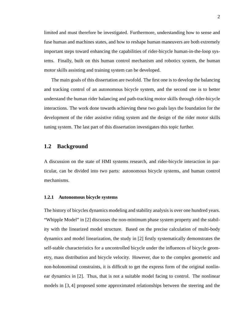
1.2.1 Autonomous bicycle systems

The history of bicycles dynamics modeling and stability analysis is over one hundred years.

“Whipple Model” in [2] discusses the non-minimum phase system property and the stabil-

ity with the linearized model structure. Based on the precise calculation of multi-body

dynamics and model linearization, the study in [2] firstly systematically demonstrates the

self-stable characteristics for a uncontrolled bicycle under the influences of bicycle geom-

etry, mass distribution and bicycle velocity. However, dueto the complex geometric and

non-holonominal constraints, it is difficult to get the express form of the original nonlin-

ear dynamics in [2]. Thus, that is not a suitable model facingto control. The nonlinear

models in [3, 4] proposed some approximated relationships between the steering and the

3

balancing torques, which can be utilized in the controller design. Furthermore, the com-

plex tire ground frictional interactions are also considered and fused into the whole system

dynamics in [5–9].

For the trajectories tracking by only using the steering andvelocity control inputs, bicy-

cle is a typical non-minimum phase underactuated system. Itis proven that no continuous

control exists for exactly tracking with keeping internal subsystem stable [10]. Feedback

linearization control methods are designed for balancing task. For example, the sliding

mode control strategy is utilized for the balancing and tracking task in [4]. Considering that

the bicycle dynamics has the external/internal convertible (EIC) structure [11], a series of

EIC-based control strategies are proposed for implementing the approximate tracking task.

First, the classic EIC-based controller is utilized for thesimplified bicycle model [11]. The

modified EIC-based control laws are designed for the complexbicycle/motorcycle mod-

els that include the special steering balancing effect and the tire ground interaction [12].

Additionally, the steering effect is proven to be able to balance a stationary bicycle [12].

However, the experimental results for this control system are inadequate comparing with

the theoretical work. The results of Blue Team in the 2005 DARPA Challenge confirm

these difficulties [13]. The recent experimental results ofprecisely trajectories tracking

are mentioned in [14]. In the recent years, Honda company proposes a motorcycle assist

system [15] that has the excellent balancing capabilities at zero or slow velocity.

To enhance the autonomous bicycle balancing and tracking capabilities and consider-

ing human rider operations, auxiliary devices are introduced and equipped on the typical

bicycle system, such as the weight lifting devices and gyro-balancers. These devices can

provide additional control inputs for internal subsystem keeping stable, and improve the

whole system balancing and tracking performances. The effect of weight shifting opera-

tion, which can be considered as the rider upper-body leaning motion, is shown to eliminate

the right half-plane zeros of the linearized closed-loop system [16]. The gyro-balancer is

another control inputs for balancing, such as the developments in [17–19]. The bikebot

4

system [14, 20] is built for the autonomous bicycle control laws implementation and hu-

man riding process observation. In [20], for the stationarybicycle, the gyro-balancer is

shown to regulate the bicycle rolling motion on a designed periodical orbit. Based on the

EIC structure, in [14], the gyro-balancer is designed as an auxiliary control for assisting the

bicycle balance and enhancing the trajectories tracking performances.

1.2.2 Human control mechanisms modeling and analysis

Modeling human control mechanisms is a complete and challenging task for several rea-

sons. Models must account for not only a non-rigid human bodyand multiple contact in-

teractions, but also complex human sensing, actuation and decision mechanisms. As much,

most research in this area focuses on the control of sitting,standing or walking motions.

For human stance, the whole or upper-body is approximately considered as an inverted

pendulum. Following the same treatment, the rider upper-body leaning motion in cycling is

modeled as an inverted pendulum swing motion [12,21,22]. This motion is one of the main

balancing sources generated by the rider. The precise dynamics model including the other

joints motion of the upper-body, arms and legs are also constructed. The work in [23] pro-

poses a physical-learning model for depicting these motions, which uses a low-dimensional

learning-based model to simulate the complex high dimensional dynamics effectively. In

most studies, only the upper-body leaning motion is considered in the system stability anal-

ysis. The rider posture estimation is necessary for the rider physical dynamics validating

and the rider control model construction. In [24, 25], the wearable inertial measurement

units (IMUs), including the accelerometers and gyroscopes, are used for the body seg-

ments orientation and position estimation. Other sensors,such as the magnetic sensor and

the onboard camera, are also introduced to enhance the measure precision and to eliminate

the IMU drifting effect [26,27].

It is challenging to capture and model human control motor skills. The motor skills

depict the combination of human sensing, decision and actuation. Several neuro-balancing

models are constructed for human stance. In [28], a time-delayed proportional-derivative

5

(PD) feedback control model is proposed. In those models, the time delayed human an-

gular positions and angular velocities are multiplied by the control gains as the balancing

joints torques. The model depicts the human sensory response to balancing states as short-,

medium- and long-latency phasic mechanisms due to proprioception, vestibular and visual

sensory. The muscle stiffness and damping factors of the neuro-musculoskeletal system are

also considered in the model. Experiments are conducted andused to validate the model

structure and identify the model parameters, the control gains and time delay constants.

However, the closed-loop system stability was not analyzedand included in [28]. A similar

simplified control model structure is used for standing on balancing board problem. Prop-

erties of the nonlinear closed-loop dynamics are discussedquantitatively, such as the limit

cycle existence and the bifurcation phenomena. The work in [29, 30] gives the qualitative

discussion of human riding behaviors, from the dynamics viewpoint and based on the ex-

perimental observation. The balance control model in [28] is also used for capturing the

stationary balancing riding in [31] and for riding stability analysis [1].

Besides balancing task, the human motor skills for complex operations are also dis-

cussed in recent years. In [32], the motion planning method is conducted on the learned

low-dimensional skill manifolds but not the complex analytical robotic models. The man-

ifold concepts are utilized for depicting the human motion sets and synergies relationships

in [33, 34]. Human motor skills learning process and behavior forming process are also

discussed, such as [35] for a kind of simulated non-minimum phase system tracking task.

However, these aforementioned works mainly focus on the human motor skills without

considering the dynamics interactions between human and machines. Few quantitative

analysis is reported for the rider path tracking with balancing maneuvers.

1.3 Dissertation outline and contributions

This dissertation is divided into eight chapters. Chapter 1is the introduction of the disser-

tation. Chapter 2 presents the bikebot system dynamics and the rider-bicycle dynamics and

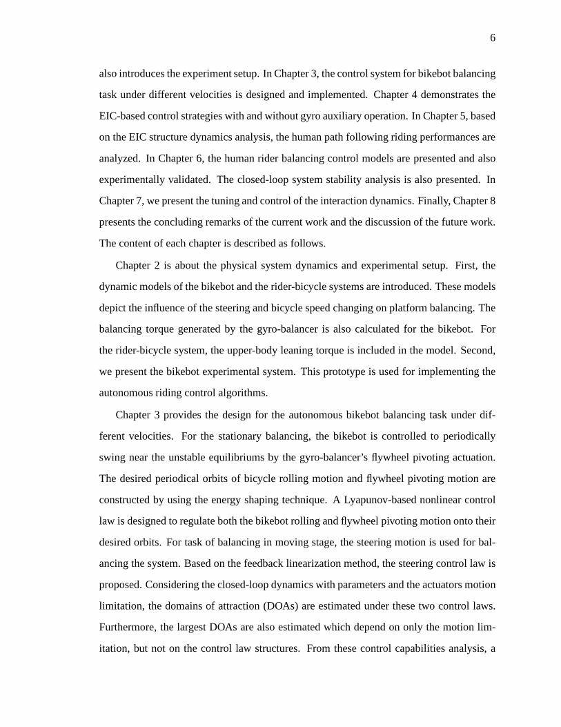
6

also introduces the experiment setup. In Chapter 3, the control system for bikebot balancing

task under different velocities is designed and implemented. Chapter 4 demonstrates the

EIC-based control strategies with and without gyro auxiliary operation. In Chapter 5, based

on the EIC structure dynamics analysis, the human path following riding performances are

analyzed. In Chapter 6, the human rider balancing control models are presented and also

experimentally validated. The closed-loop system stability analysis is also presented. In

Chapter 7, we present the tuning and control of the interaction dynamics. Finally, Chapter 8

presents the concluding remarks of the current work and the discussion of the future work.

The content of each chapter is described as follows.

Chapter 2 is about the physical system dynamics and experimental setup. First, the

dynamic models of the bikebot and the rider-bicycle systemsare introduced. These models

depict the influence of the steering and bicycle speed changing on platform balancing. The

balancing torque generated by the gyro-balancer is also calculated for the bikebot. For

the rider-bicycle system, the upper-body leaning torque isincluded in the model. Second,

we present the bikebot experimental system. This prototypeis used for implementing the

autonomous riding control algorithms.

Chapter 3 provides the design for the autonomous bikebot balancing task under dif-

ferent velocities. For the stationary balancing, the bikebot is controlled to periodically

swing near the unstable equilibriums by the gyro-balancer’s flywheel pivoting actuation.

The desired periodical orbits of bicycle rolling motion andflywheel pivoting motion are

constructed by using the energy shaping technique. A Lyapunov-based nonlinear control

law is designed to regulate both the bikebot rolling and flywheel pivoting motion onto their

desired orbits. For task of balancing in moving stage, the steering motion is used for bal-

ancing the system. Based on the feedback linearization method, the steering control law is

proposed. Considering the closed-loop dynamics with parameters and the actuators motion

limitation, the domains of attraction (DOAs) are estimatedunder these two control laws.

Furthermore, the largest DOAs are also estimated which depend on only the motion lim-

itation, but not on the control law structures. From these control capabilities analysis, a

7

switching control strategy is proposed for balancing in thestationary-moving stages transi-

tion process. The experiments results demonstrate the performances of the aforementioned

control methods.

Chapter 4 focuses on the bikebot autonomous tracking tasks.First, using the steering

properties of the EIC structure, we present a tracking and balancing control strategy. The

tracking and balancing errors analysis is then discussed. Considering the non-minimum

phase system property, an auxiliary gyro pivoting control law is designed for reducing the

path tracking errors. The tracking performance of these twocontrol methods are demon-

strated by both the analysis and the experiments. The EIC-based control with modified

velocity vector field is also implemented.

Chapter 5 presents the analyzing methods and results about the human rider path track-

ing and balancing performance. Based on the EIC structure, the balance equilibrium man-

ifold (BEM) concept is introduced. Based on the BEM concepts, we first analyze the

balancing contribution of the steering and the upper-body leaning operations. The analysis

shows that using the steering actuation is much more effective than the body movement

in term of platform balance task. A balancing metric is also defined for measuring the

balancing performance along the rider tracking process. A second metric is introduced for

depicting the tracking and balancing results of riders. Finally, multiple riders are asked to

control the bikebot to track the given paths. These rider experiments results are used to

demonstrate the effectiveness of the proposed analyzing methods.

In Chapter 6, the human balance skills are discussed. Based on the recorded data from

the conducted balance riding experiments, the control models of steering operation and

upper-body leaning torque are constructed and proposed in this chapters. Both control

models share the time delayed PD feedback structures with the bicycle frame and the upper-

body rolling information. We then discuss the stability analysis of the linearized closed-

loop system. For the stability and balancing performances,the influence of the changing of

the dynamics physical parameters, the control gains and time delays in the human control

8

models are also discussed. Extensive experiments are conducted by multiple subjects, un-

der different types disturbances, the rolling torque perturbation by gyro pivoting, the visual

feedback channel disturbance and the additional time delayon the steering actuator. We

analyze these experimental results and present the human balance motor skill changes.

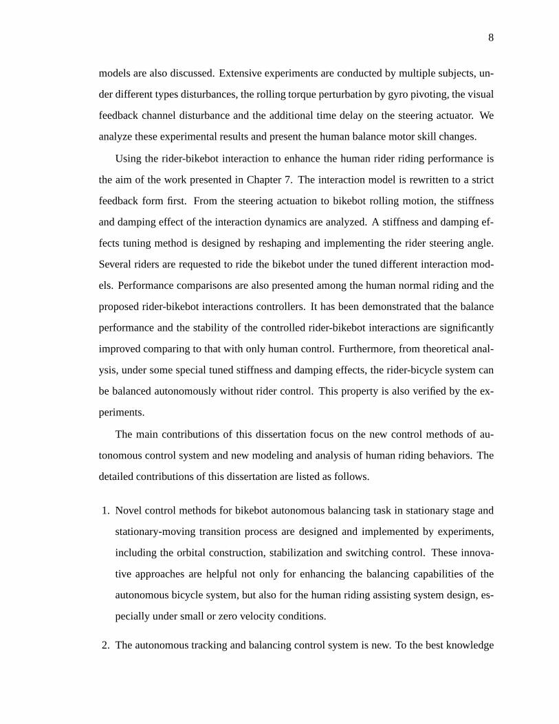
Using the rider-bikebot interaction to enhance the human rider riding performance is

the aim of the work presented in Chapter 7. The interaction model is rewritten to a strict

feedback form first. From the steering actuation to bikebot rolling motion, the stiffness

and damping effect of the interaction dynamics are analyzed. A stiffness and damping ef-

fects tuning method is designed by reshaping and implementing the rider steering angle.

Several riders are requested to ride the bikebot under the tuned different interaction mod-

els. Performance comparisons are also presented among the human normal riding and the

proposed rider-bikebot interactions controllers. It has been demonstrated that the balance

performance and the stability of the controlled rider-bikebot interactions are significantly

improved comparing to that with only human control. Furthermore, from theoretical anal-

ysis, under some special tuned stiffness and damping effects, the rider-bicycle system can

be balanced autonomously without rider control. This property is also verified by the ex-

periments.

The main contributions of this dissertation focus on the newcontrol methods of au-

tonomous control system and new modeling and analysis of human riding behaviors. The

detailed contributions of this dissertation are listed as follows.

1. Novel control methods for bikebot autonomous balancing task in stationary stage and

stationary-moving transition process are designed and implemented by experiments,

including the orbital construction, stabilization and switching control. These innova-

tive approaches are helpful not only for enhancing the balancing capabilities of the

autonomous bicycle system, but also for the human riding assisting system design, es-

pecially under small or zero velocity conditions.

2. The autonomous tracking and balancing control system is new. To the best knowledge

9

of the author, no such experiments have been reported in the past.

3. The human riding behaviors for balancing and tracking tasks are systematically col-

lected, observed and analyzed under designed experiments conditions with multiple

types of disturbances. Based on this work, the human balancing motor skills are ana-

lyzed. These experiments and methods are new.

4. The human rider control models for balance riding are proposed and validated. This

work provides in-depth understanding of human riding control mechanism, and a novel

compensation method for general balancing mechanism studyand the human-in-the-

loop system design.

5. The rider tracking with balancing control skills are analyzed. We present new BEM

concepts and metrics for measuring the rider performances.These metrics are new and

can be used to capture and characterize the motor skills. TheEIC-based evaluation

indexes and the analyzing tool give the guidance for the rider assisting system design.

Furthermore, these methods can also be extended to other human-machine interaction

analysis, especially for the unstable control system.

6. A novel rider-bikebot interaction tuning method is designed and implemented in experi-

ments. The method can effectively enhance the human rider riding safety and balancing

performances. The proposed interaction tuning methodology has a potential value for

riding training system design. To the best knowledge of the author, riding balance

tuning design and experiments have not been reported in the past.

10

Chapter 2

System Dynamics and Experiment System

2.1 Introduction

For understanding the rider-bicycle system interaction and enhancing the autonomous bi-

cycle system capability, the dynamic model construction isan important and foundational

work. For validating the rider-bicycle interaction analysis, implementing the autonomous

control system and assisting/perturbing the rider behaviors, building an autonomous bicy-

cle experimental system is necessary and critical.

Lots of works have been done to depict the dynamics of the moving motorcycle and

bicycles, including the special geometry structure and thetire-road interaction [12]. Based

on the no-slipping and no-sliding assumption, the non-holonomic constraints are intro-

duced, and the Whipple model is constructed for the moving bicycle utilizing multi-body

Lagrangian equations [29]. Some self-stability properties are demonstrated under different

geometrical and mass distribution parameters [2, 36]. Besides, the tire-road friction model

is combined under the slipping and sliding condition [3]. Considering the lateral motion of

the tire-ground contact point, the stationary motorcycle dynamics with an accurate steer-

ing mechanism is proposed in [37]. The bikebot system with gyro-balancer dynamics is

also constructed in [14, 37], with the analysis of coupling effect from flywheel pivoting

motion with bicycle frame rolling motion. Furthermore, combining the bicycle dynamics

with the rider body motion, the rider-bicycle system dynamics is also studied in recent

years. In [21, 22], the rider upper-body is considered as an inverted pendulum mounted on

the bike seat, and the upper-body leaning motion is considered as an important motion for

balancing.

11

The first part of this chapter demonstrates the rider-bicycle dynamics, and autonomous

bikebot dynamics, which are mentioned in [21, 22] and [14, 20], respectively. Comparing

with other rider-bicycle dynamic models, the rider upper-body leaning torque, the main

balancing torque generated by riders, are picked up and calculated in the dynamics. For the

bicycle part, some different kinds of balancing torques resulting from steering are also in-

cluded. The second part focuses on the experiment system, which is mentioned and utilized

in the works of [14, 20–22]. The functions and design detailsof sensing, data processing

and actuating are included. It has to be pointed out that, thedynamics construction works

are from the cooperation of this dissertation author and hisresearch group colleague Dr.

Yizhai Zhang, and for the experiment system, the author focuses on the redesign and mod-

ification works about the sensors, programs and actuators. The original bikebot design is

proposed by colleague Dr. Yizhai Zhang [12]. Considering the whole work completeness

and without repeating to mention these backgrounds, the dynamics and experimental sys-

tem are proposed in this chapter as the preparing and basic work of the entire dissertation

work.

The rest part of this chapter is organized as follows. The bikebot dynamics and rider-

bicycle system dynamics are introduced in Section 2.2 and 2.3, respectively. Section 2.4

demonstrates the experimental system. The conclusion is listed in Section 2.5.

2.2 Bikebot system dynamics

As shown in Fig. 2.1(a), the bikebot system can be consideredas several inter-connected

parts: the rear frame with the rear wheel, the gyro-balancermounted on the rear frame, and

the front wheel. There are three coordinate frames are introduced for motions and attitude

descriptions: the fixed inertial frameN , the translating and rotating body frameB, and the

translating trajectory frameR. As shown in Fig. 2.1(b), the origin ofR frame is attached

at the rear wheel contact pointC2 with x-axis parallel with the wheel baseC1C2, which is

defined as the straight line connecting the front wheel contact pointC1 and the rear wheel’s

12

CompactRIO embed. sys. motor

GPSantenna

Gyro−balancer

Bikebot IMU

High−precision antenna

Steering motor

Driving

(a)

Gyro−balancer

xryr

zr

xbybzbϕb

ϕw

ψ

φg

φ

lb

hb

l

ωs

ξ

W

C1

C2

G

B

RNXY Z

ϕw

(b)

Figure 2.1: (a) The Rutgers bikebot system. (b) A kinematic schematic of the gyro-balanced bikebot system.

C2. TheC2 velocity alongxb is defined asvr. Thez-axis of frameR is parallel with the

z-axis ofN . Bikebot roll angle, the angle between thez-axis ofB andz-axis ofN , is

defined asϕb. The yaw angleψ is defined as the angle between thex-axis ofN andx-axis

of R. The horizontal and vertical positions of the mass center point G with respect toBarelb andhb, respectively. The bicycle mass and mass moment of inertia aboutG point in

the direction of thex-axis ofB aremb andJb, respectively. The length of wheel baseC1C2

is denoted asl. And the front wheel caster angle is denoted asξ, and the front wheel trail

distance is denoted aslt. With the steering angleφ, the projective steering angle on the

ground isφg, which can be calculated as1

φg = arctan

(tanφ cξ

cϕb

)

.

As the same treatment in [22], the relationships betweenψ andφ are

ψ =vr tanφ cξl cϕb

(2.1)

and

uψ =vr cξl cϕb

(

sec2φ φ+ tanφ tanϕbϕb

)

+vr tanφ cξl cϕb

(2.2)

with defininguψ = ψ.

1Notationcx = cosx(sx = sinx) for variablex is used through the entire dissertation.

13

Combining the rolling and the yawing motion, the center masspoint linear velocity

vectorvg w.r.t. N expressed inB is

vG =(

vr − hbψ sϕb

)

ib +(

hbϕb + lbψ cϕb

)

jb − lbψ sϕb kb (2.3)

with ib, jb andkb as the unit vectors of thexb-, yb- andzb-axes ofB, respectively.

The height of the center mass is mainly dominated by the rolling motion by the term

hbcϕb . Furthermore, at smallϕb case, another height changing factor∆hb has to be consid-

ered due to the combination of rolling and steering, which can be approximated as

∆hb ≈ltlb cξ tanφ sϕb

l. (2.4)

Thus, the potential energyV is

V = mbg

(

hb cφb −ltlb cξ tanφ sϕb

l

)

. (2.5)

The pivoting angle of the spinning flywheel isϕw along they-axis ofB, and the spin-

ning angular velocity isωs. Another pivoting coordinate frameF is introduced, in which

they- andz-axes are accorded by the definitions ofϕw andωs, respectively.if , jf andkf

are the unit vectors of thex-, y- andz− axes directions inF . Thus, the angular velocity

vectorωf w.r.t toN expressed inF is

ωf =(

cϕw ϕb − sϕw cϕb ψ)

if +(

sϕb ψ + ϕw

)

jf+(

sϕw ϕb + cϕw cϕb ψ + ωs

)

kf . (2.6)

Let Iz be the mass moment of inertia of the flywheel along the spinning axis. Naturally, the

mass momentum of inertia along they- andx-axes ofF , Ix andIy are approximated asIz2

.

The inertia matrixIw expressed inF is Iw = diagIz2, Iz

2, Iz

.

The total kinematic energyT is obtained as

T =1

2mbv

TGvG +

1

2Jbϕ

2b +

1

2ωTf Iwωf . (2.7)

The balancing dynamics along thex-axis ofB has the general coordinatesq = [ϕb, ϕw]T

under the controlled pivoting torqueτp. After defining the LagrangianL = T − V , the

Lagrangian equation is utilized for the dynamics construction

d

dt

(∂L

∂qi

)

− ∂L

∂qi= ui, i = 1, 2, (2.8)

14

with u1 = 0, u2 = τp. From (2.8), we obtain the equation of motion

(mbh

2b + Jb + Iz s2

ϕw + Iz2

c2ϕw

)ϕb +mbhb cφb vrψ −mbh

2b cϕb sϕb ψ

2

−mbgltlb tanφ cξ cϕbl

−mbhbg cϕb −mbhblb cϕb uψ

+Iz cϕw

(

ωs − 12ϕb sϕw −1

2ψ cϕb cϕw

)(

ϕw − cϕb ψ)

= 0

(2.9)

andIz2ϕw + Iz c2

ϕwcϕb ψϕb + Iz

2cϕw sϕw ϕ

2b − Iz

2cϕw sϕw c2

ϕbψ2

+Izωs

(

ψ cϕb sϕw −12ϕb cϕw

)

− Iz2

sϕb uψ = τp.(2.10)

The trajectory motion kinematics is calculated as follow. The 2-dimensional position

of rear wheel contact pointC2 is defined asrC2 = [X, Y ]T in N , with velocityvC2 = rC2 .

Under the non-holonomic constraint ofC2, the lateral velocity is zero and the velocityvC2

has the relationship withvr andψ as

vC2 =

vX

vY

=

X

Y

=

cψ − sψ

sψ cψ

vr

0

. (2.11)

After taking twice derivatives, under the control inputu = [ur, uψ] with ur = vr, the

dynamics extension results in

r(3)C2

= vC2 = −

2vr sψ +vrψ cψ

−2vr cψ +vrψ sψ

ψ

︸ ︷︷ ︸

Ψ

+

cψ −vr sψ

sψ vr cψ

︸ ︷︷ ︸

Rψ

u. (2.12)

2.3 Rider-bicycle system dynamics

For the rider-bicycle system, the kinematics of the trajectory motion is same as that of the

aforementioned bikebot system. Only the rolling dynamics is given in this section, which

is also similar as the former system.

As shown in Fig. 2.2(b), the rear frame and steering structures of the rider-bicycle

system are the same as the bikebot in Fig. 2.1(b). The flywheelpart is not considered in the

dynamics. One main difference is that the upper-body motionis considered. Naturally, the

upper-body with arms has multiple DoFs. However, only the upper-body leaning motion

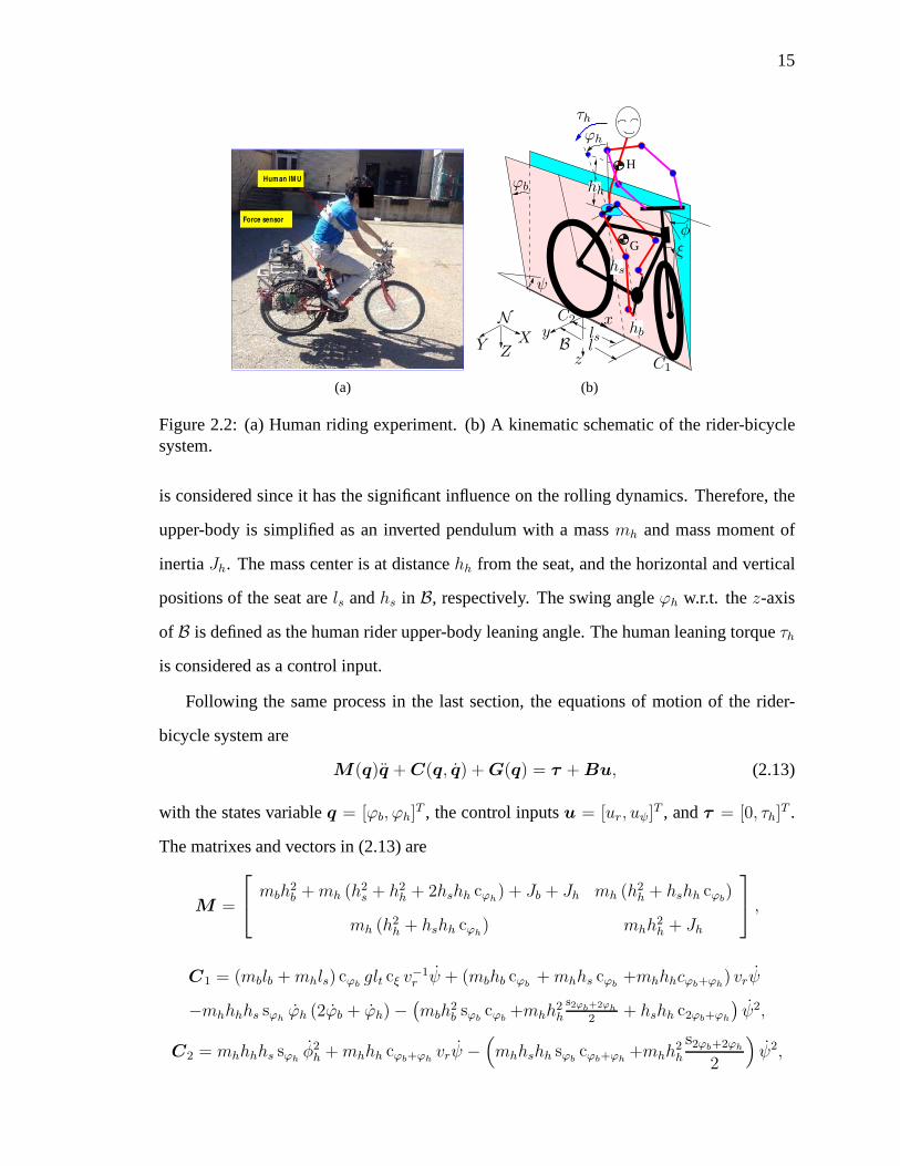
15

Human IM U

Force sensor

(a)

G

H

XY Z

x

z

y

hs

τh

ϕb

N

C1

C2

l

hh

hbls

ψ

ϕh

B

φ

ξ

(b)

Figure 2.2: (a) Human riding experiment. (b) A kinematic schematic of the rider-bicyclesystem.

is considered since it has the significant influence on the rolling dynamics. Therefore, the

upper-body is simplified as an inverted pendulum with a massmh and mass moment of

inertiaJh. The mass center is at distancehh from the seat, and the horizontal and vertical

positions of the seat arels andhs in B, respectively. The swing angleϕh w.r.t. thez-axis

of B is defined as the human rider upper-body leaning angle. The human leaning torqueτh

is considered as a control input.

Following the same process in the last section, the equations of motion of the rider-

bicycle system are

M(q)q + C(q, q) + G(q) = τ + Bu, (2.13)

with the states variableq = [ϕb, ϕh]T , the control inputsu = [ur, uψ]

T , andτ = [0, τh]T .

The matrixes and vectors in (2.13) are

M =

mbh

2b +mh (h2

s + h2h + 2hshh cϕh) + Jb + Jh mh (h2

h + hshh cϕb)

mh (h2h + hshh cϕh) mhh

2h + Jh

,

C1 = (mblb +mhls) cϕb glt cξ v−1r ψ + (mbhb cϕb +mhhs cϕb +mhhhcϕb+ϕh) vrψ

−mhhhhs sϕh ϕh (2ϕb + ϕh) −(mbh

2b sϕb cϕb +mhh

2h

s2ϕb+2ϕh

2+ hshh c2ϕb+ϕh

)ψ2,

C2 = mhhhhs sϕh φ2h +mhhh cϕb+ϕh vrψ −

(

mhhshh sϕb cϕb+ϕh +mhh2h

s2ϕb+2ϕh

2

)

ψ2,

16

G =

−mbhbg sϕb −mhhsg sϕb −mhhhg sϕb+ϕh

−mhhhg sϕb+ϕh

,

and

B =

0 −mbhblb cϕb −mhhslh cϕb −mhhhlh cϕb+ϕh

0 −mhhhlh cϕb+ϕh

.

2.4 Bikebot experiments system

Fig. 2.3 shows the bikebot experiment system, that can be ride by human rider or controlled

by the onboard computer. The bikebot system is designed and built for three aims. The first

aim is recording the rider operation and system states, and generating disturbances into the

rider’s closed-loop sensorimotor feedback system. The second one is experimentally val-

idating the designed autonomous bikebot balancing and tracking controllers. The last one

is to tune the human behaviors for enhancing the riding safety and efficiency and training

the human riders.

IMU

embed. sys. CompactRIO

Hub−motor

Gyro−balancer sensor

actuator Brake

encoder Handlebar 6−DoF force

Crank/pedal encoders

Steering

encoder

Flywheel

mechanism

Wheel

Figure 2.3: The Rutgers bikebot.

This platform is modified from a mountain bicycle with added onboard sensors and

actuators. As shown in Fig. 2.4(a), a real-time embedded system (from NI cRIO model

9082) is used for collecting the sensor measurements and also for motion control. For the

sensing part, the bicycle velocityvr is obtained by the encoder mounted on the rear wheel;

the steering angleφ and the handlebar rotating angleφh are measured by two encoders on

17

(a) (b)

Figure 2.4: (a) Bikebot data onboard control system. (b) 6-DoFs IMU.

(a) (b)

Figure 2.5: (a) Gyro-balancer part. (b) Autonomous steering part.

the steering structure, and the upper-body relative leaning angleϕh is captured by a rolling

arm equipped with an encoder that is connected to the upper body. In the gyro-balancer

subsystem (Fig. 2.5(a)), the flywheel pitching and spinningangles are measured by the en-

coders. Besides, the bicycle and upper-body 6-DoFs motion information, includingϕb, ϕh

andψ, are detected by two IMUs attached on them. The bicycle frame-fixed IMU is shown

in Fig. 2.4(b). The bicycle position is measured by the onboard GPS system, or calculated

by the measured steering angleφ and bicycle speedvr along the riding trajectory.

For the actuation parts, the pedaling actuation is powered by a motor through the on-

board computer system, while a human rider can still manually control it. As shown in

18

Fig. 2.5(b), the front wheel can be configured either mechanically connected or discon-

nected to the handlebar. On one hand, like a normal bicycle, the bicycle steering operation

can be carried out directly by the rider through the handlebar. On the other hand, when the

front wheel is mechanically disconnected with the handlebar, the steering motion is driven

by the steering motor directly. This function provides the capability that the actual steer-

ing angle can be controlled to follow a designed profile. For the rolling torque generated

by the gyro-balancer subsystem (Fig. 2.5(a)), the pitchingangle and spinning speed of the

flywheel are independently controlled by two motors.

2.5 Conclusion

The dynamics models of the bikebot system and the rider-bicycle system were proposed in

this chapter. The control effects of steering, gyro-balancing torque, and rider upper-body

leaning motion were demonstrated in these models. The bicycle experimental system was

also demonstrated, in which the states measuring and recording, control processer, and the

actuators were introduced.

19

Chapter 3

Bikebot Autonomous Balancing Control

3.1 Introduction

Bicycles and motorcycles provide an excellent platform forstudying human-machine or

human-robot interactions. It has also been reported for clinical diagnosis and rehabilitation

treatment [38–40]. In [20], an actively controlled bicycle-based robot, called bikebot, is

designed to study human neuro-control mechanism and physical human-robot interactions.

Due to its non-minimum phase dynamics, it is challenging to design bikebot control sys-

tem. From practice viewpoint, it is desirable to have a complete autonomous strategy for

the bikebot system from stationary to moving maneuvers. However, because of different

bikebot dynamics at stationary and moving speed, the platform balance strategies are not

the same. The goals of this chapter are to design the balance control laws under stationary

and moving conditions, and to develop an integrated stationary and moving balance control

for autonomous bikebot.

Dynamics and control of bicycles or motorcycles are among active research areas for

many years [16]. Autonomous single-track vehicles need to maintain both trajectory track-

ing and platform balancing tasks simultaneously. Using thesteering and velocity actua-

tions, several controller designs were developed [11,14,41–43]. An elegant design in [11]

takes advantage of the EIC dynamics structure of the riderless bicycle to design an au-

tonomous controller. A simplified bicycle model is used in [11] and only simulation results

are presented to illustrate the design methodology. The work in [14] extends the EIC-based

control design and demonstrates the experimental implementation and performance using

the bikebot. Other experimental and demonstration works include those in [14,42,44,45].

20

The stationary balance control is also a difficult task for the bikebot system. The ad-

ditional rolling torque generated by the gyro-balancer canbe used for the balance keeping

task. In recent years, control laws are proposed for balancing similar systems, such as the

inverted pendulum, Furuta pendulum and acrobat system [46,47]. These controllers can be

divided into two groups: the equilibrium point regulation and orbital regulation. The typ-

ical method of the former is the energy shaping and dissipation injection design [48–51].

The latter design is sophisticated with two parts: the orbitconstructing and regulation con-

trol design. The first part is orbits existence, that is, the target orbit of the system states

should be related and they are the solutions of the closed-loop dynamics. Virtual con-

straints [52,53], sliding modes [4] or limit-cycle dynamics [54] are introduced, and the sys-

tem dynamic forms are dominated by the conservation of the first integral. The regulation

control law can then drive the states onto their target orbits [55], such as time varying lin-

ear feedback control methods with transverse dynamics [56]. In [20], using gyro-balancer,

an orbital regulation control law is proposed to balance theplatform at stationary or low

moving velocities.

It is challenging to estimate the maximum roll motion range under a certain control

system. The results in [57] show that the bicycle can only be stabilizable within a small

range of roll angles (e.g., 1-2 degs), particularly at low moving velocities. The simple

analysis in [37] has showed that balancing a stationary bicycle only by steering actuation

is extremely difficult because of a small DOA under the controller design. Introducing

additional actuators can overcome this limited stabilizable range and assist the balance

capability. However, no formal analysis is given to estimate the DOA under the control

design in [20].

In this chapter, the gyro-balancer control law is proposed first for the stationary bal-

ance control task. In this task, the orbital regulation is chosen as the control method. That

is, the stationary bicycle is expected not only to keep balance but also to swing near the

equilibrium point periodically controlled by the gyro-balancer pivoting motion. The en-

ergy shaping techniques is utilized for shaping the desireddynamics as a simple pendulum

21

dynamics. The virtual constraint between the bikebot rolling angle and flywheel pivoting

velocity is built to get the desired periodical orbits for the bikeobt frame rolling and fly-

wheel pivoting motion. According to the reshaped energy andproposed virtual constraint,

a Lyapunov-based orbital regulation controller is designed. The theoretical stability analy-

sis and experimental results demonstrate that the system states can converge to the desired

orbits. It has to be pointed out that for the first time the gyro-balancer stationary balancing

control experiment is carried out by the author and Dr. Yizhai Zhang, and other parts in this

chapter are completed by the author himself. For balancing of a moving platform, based

on the feedback linearization structure, the steering balancing control law is introduced.

We then present an integrated stationary/moving balance control of autonomous bike-

bots. The control system integrates the balance control strategies for the stationary and

moving bikebot platform. Due to different dynamics and control design for stationary and

moving bikebot, we analyze the DOAs for the given controllers and then a switching strat-

egy is used to integrate them for stationary-to-moving and moving-to-stop maneuvers. The

integration design guarantees that the transition state lies in the DOAs of the closed-loop

dynamics under the targeted control design. To demonstratethe DOA analysis and integra-

tion design, we use the orbital regulation control law [20] for balancing stationary bikebot

and the EIC-based balance control is used for the moving bikebot [22]. Furthermore, a fea-

sible DOA concept is introduced to capture the possibly largest state variable region under

any balance control laws with consideration of actuation limits. The main contribution of

work lies in the analysis and design of the integrated balance control for the autonomous

bikebot in the stationary-moving transition. The switchedcontrol design provides guaran-

teed balance performance and could be used for other underactuated balance robots.

The rest parts of this chapter are organized as follows. Section 3.2 focuses on the task

of balancing under only gyro pivoting control design, including the orbits construction and

orbital regulation control. Section 3.3 introduces a steering balancing control for moving

stage. The control capacity analyses, the DOA estimates, and the switching control design

22

are presented in Section 3.4. Section 3.5 demonstrates the experimental results and pro-

vides the control performance analysis. Section 3.6 gives the conclusion of the works in

this chapter.

3.2 Stationary balancing by gyro-balancer

This section focuses on the stationary bicycle balancing bythe gyro pivoting control. First,

an orbits constructing method is proposed, and then the orbit regulation controller with

stability analysis is demonstrated. Finally, the control system performance is shown by the

experiment results.

3.2.1 Orbits construction

Under conditionsvr = 0 andφ = 0, the bikebot dynamics (2.9) and (2.10) reduce to(

mbh2b + Jb + Iz s2

ϕw +Iz2

c2ϕw

)

ϕb −mbhbg sϕb +Iz

(

ωs −1

2ϕb sϕw

)

cϕw ϕw = 0, (3.1)

andIz2ϕw +

Iz2

cϕw cϕw ϕ2b −

1

2Izωs cϕw ϕb = τp. (3.2)

Noticing (3.2) without the coupling term ofϕb, the pivoting angular velocityϕw can be

easily controlled to track the desired trajectories through a lower level tracking controller.

Thus, these dynamics can be modified into a 3-dimensional system as

x1 = x2 (3.3a)

x2 = f(x) + g1(x)u1 (3.3b)

x3 = u1, (3.3c)

with the statesx = [x1, x2, x3]T = [ϕb, ϕb, sϕw ]T , the control inputu1 = cϕw ϕw, and

f(x) =mbghb sx1

mbh2b + Jb + Iz s2

ϕw + Iz2

c2ϕw

, g1(x) = − Ixx2 s2x3 +Izωs

mbh2b + Jb + Iz s2

ϕw + Iz2

c2ϕw

.

Due to the mechanical structure constraints, the pivotingϕw andϕw are bounded as

|x3| = | sϕw | ≤ sϕmaxw

< 1, |u1| = | cϕw ϕw| ≤ ωmaxw

23

with the maximum pivoting angle and angular velocity asϕmaxw andωmax

w , respectively. The

equilibrium of the dynamics (3.3) isx1e = x2e = 0 underϕwe = 0.

Furthermore, the rolling dynamics (3.2) satisfies

d

dt

[(mbh

2b + Ix)x2 + Ixx1x

23 + Izωsx3

]= − ∂

∂x1(mbghb cx1) (3.4)

with the angular momentum along thex-axis as

px(t) = (mbh2b + Ix)x2(t) + Iwxzx2(t)x

23(t) + Iwzωsx3(t). (3.5)

By integrating (3.4), the angular momentum is

px(t) − px(0) =

∫ t

0

mbghb sx1(τ) dτ. (3.6)

Thus, the following property is introduced.

Property 3.1. For a given periodic profilex1(t) with periodT , the profile for the pivoting

angle is also periodic with the same period.

Proof. Given an arbitrary periodical orbitx1(t + T ) = x1(t) for any t, x2(t) = x1(t) is

also periodic with periodT , i.e.,x2(t+ T ) = x2(t). And then, the following relationships

are obtained

px(t+ T ) − px(0) =

∫ t+T

0

mbghb sx1(τ) dτ

and

px(t+ T ) − px(t) =

∫ T

0

mbghb sx1(τ) dτ. (3.7)

Under periodicalx1(t) andx2(t),∫ T

0sx1(τ) dτ = 0. Therefore, (3.4) reduces to

[x3(t+ T ) − x3(t)] [Iwzωs + Iwxz(x3(t+ T ) + x3(t))] = 0.

Thus,x3(t+ T ) = x3(t) andϕw is also periodic with periodT .

In the following, the orbits construction method based on energy shaping mechanism

is demonstrated. First, the rolling dynamics (3.3b) is simplified, considering the facts that

ωs ≫ |x2|, Izωs cx3 ≫ |Ixx2 s2x3 | andmbh2b ≫ Ix. Thus,

x2 −g

hbsx1 +

Izωsmbh2

b

u1 = 0, (3.8)

24

with x ∈ D := S × R × (−1, 1). The desired bicycle rolling orbitOb is then designed as

the following simple pendulum dynamics profile as

Ob : x2 +b

hGsx1 = 0 (3.9)

with a gravitationally equivalent constantb > 0 and a given initial valuex10. When the

rolling statesx1 andx2 are onOb, the controlledx3 has to satisfy the relationship as

x3 = −(b+ g)mbh2b

Iwzbωsx2 = −Lx2 (3.10)

with constantL =(g+b)mbh

2b

Izbωs. For obtaining the large control actuator pivoting range, the

desired flywheel pivoting orbitOw is designed as the integration of (3.10) with zero initial

values. Therefore,Ow is designed as

Ow : x3 = −Lx2, (3.11)

which can be also considered as a virtual constraint for the system statesx1 andx3.

In fact, the orbits structures (3.9) and (3.11) provide a family of orbits with the same

dynamics form. To determine the final orbits, the initial states values are needed. Here, the

defined energy function is introduced for choosing a unique orbit in Ob, that is, the total

energy under the definedb, as

E(x1, x2) =1

2mbh

2bx

22 +mbhbb (1 − cx1) . (3.12)

When target orbitOb reaches the maximum anglexd1 with x2 = 0, the total energy is

Ed = mbhbb(1 − cxd1). Thus, the dynamics (3.9) and (3.11) withEd generate a unique

orbits coupleOb andOw.

Remark 3.1. The proposed orbits construction process is similar as the classic method

in [53,56]. However, there are two main differences comparing these two strategies, which

are dominated by the special dynamics form of the bikebot system. First, the construction

steps are not the same. In the proposed method, the orbit shape, as (3.9), is designed

firstly, and the virtual constraint (3.11) is obtained usingthe orbit shape. That is, the

25

energy shaping progress is to determine the dynamics to a desired form. Contrary to the

presented approach, the method in [53, 56] takes a reverse order in design. Second, the

virtual constraints are not the same. The proposed method isa linear relationship between

the angular velocityϕb and the angular positionϕw, not as that among the position states.

That is due to the dynamics model structure. The coupling term is only in the centripetal-

Coriolis torque, but not in the potential and acceleration terms.

3.2.2 Orbital regulation controller design

For regulating the system states on the desired orbits, the control law is proposed as follows.

The control inputu1 is designed as

u1 =Lb

hb(sx1 +v1) . (3.13)

And the auxiliary control inputv1 defined as

v1 = k2 [∆Ex2 + αk1 (x3 + Lx2)] , (3.14)

with constantα = gbIzωs

and the energy difference∆E = E(x1, x2) − Ed under given

desiredEd.

Property 3.2. Starting at a given non-zero statex0, statex of dynamics (3.3) and (3.8) can

be asymptotically regulated onto the desired orbits (3.9) and (3.11) with desireEd, under

the designed controller (3.13) and (3.14).

Proof. The positive defined Lyapunov candidate functionV1(x) is designed as follows

V1(x) =1

2∆E2 +

1

2k1 (x3 + Lx2)

2 (3.15)

with the positive constantk1. Its time derivative is

V1(x) = ∆E(mbh2bx2x2 +mbhbbsx1x2) + k1(x3 + Lx2)(x3 + Lx2). (3.16)

Substituting the dynamics (3.3b) and the designed controller (3.13), (3.16) becomes

V1(x) = −mbhb(g + b) [∆Ex2 + αk1 (x3 + Lx2)] v1. (3.17)

26

Consideringv1 structure in (3.14),V1(x) is not greater than zero, as

V1(x) = −mbhb(g + b)k2 [∆Ex2 + αk1 (x3 + Lx2)]2 ≤ 0. (3.18)

Based on (3.18), according to LaSalle theory [58],x can be proven to converge to the

invariant setS(x) asymptotically,

S(x) =x ∈ D |∆Ex2 + αk1 (x3 + Lx2) = 0

. (3.19)

It is obvious that the origin point is in the set, asxe = 0 ∈ S(x). At this point,x = 0. For

any none zero states point inS(x), the auxiliary control inputv1 is zero, and the desired

orbit dynamics (3.9) is satisfied. That is, the energy difference∆E is a constant value, and

integrating from (3.10), the virtual constraint value ofx3 + Lx2 is constant.

If ∆E 6= 0, considering non-constantx2 on (3.10), with the constantx3 + Lx2, the

equationv1 = 0 can not be satisfied. It exists a contradiction. Thus,∆E = 0 and the set

Ow = S(x) \ 0 also satisfies

Ow(x) = x ∈ D |∆E = 0, x3 + Lx2 = 0 . (3.20)

That is equivalent to the desiredOb andOw with E = Ed.

3.3 Balancing control by steering actuation

We consider to use steering actuation to balance the platform under moving velocityvr > 0.

From the bikebot dynamics, the balance torqueτs generated by steering is calculated as

τs = (kp1 + kp2φt)φt + kdus (3.21)

with φt := tanφ, andus := φt as the controlled steering angular velocity.kp1 =mbhb cξ

l(v2r−

v2c ), vc =

√glblt cξhb

, kp2 = −mbh2bv

2r c2ξ tanϕb

landkd =

mbhblbvr cξl

. Note that the sign of pa-

rameterkp1 depends on the velocityvr andkd > 0. It is straightforward to obtain that

with increasing steering angleφ and velocityvr, the torqueτs value grows as well. It is

noted that when bikebot velocityvr is small, the value of torqueτs is small. Because of this

27

observation, it is extremely challenging to use steering actuation to balance the platform

whenvr is small. Therefore, the following design is for relative large velocityvr ≥ vc.

Using the feedback linearization, the steering control input us can be designed as same

as the EIC-based control strategy [14] and also in Chapter 4.For a given moving trajectory,

we can calculate the balance equilibrium manifold and letϕbe denote the desired roll angle.

The balance errors are denoted aseϕb = ϕb − ϕbe, eϕb = ϕb − ϕbe, andeϕb = ϕb − ϕbe.

Under fixed flywheel pivotingϕw = ϕw = 0 andωs = 0, uw = 0, (2.9) is approximately

reduced to

Jtϕb ≈ fs − kdus,

with fs = mbghbsϕb − kp1 tanφ− kp2 tan2 φ, Jt = mbh2b + Jb + Iz and the approximation

of uψ asuψ ≈ vr cξl cϕb

us. The steering control inputus is designed as

us =1

kd[fs + Jt(c1eϕb + c0eϕb)] , (3.22)

where constantsc1, c2 > 0. The closed-loop dynamics is theneϕb + c1eϕb + c0eϕb = 0,

which is obviously asymptotically stable.

3.4 Balance switching control laws

In this section, we present the balance capacity and comparison between the gyro-balancer

and the steering actuation first. The main goal of this comparison is to explain and jus-

tify the use of each of these two actuators for balance control. From this analysis, it

becomes clear that the gyro-balancer can effectively be used for stationary bikebot bal-

ance (small steering-induced torque), while the steering balance torque would dominate

the gyro-balance torque at relatively large moving velocities. Because of this observation,

we consider that at stationary or low velocity, the balance is maintained by the gyro-balance

only and at relatively large velocities, only steering balance is used. For a complete design,

a switching control strategy is needed, that is, the gyro-balancer and steering actuation

are used for balance control at different velocity ranges. The switching conditions are de-

termined by the control capacity of each actuation. The estimated DOA is an effective

28

measure for quantifying control capacity.

3.4.1 Balancing actuation capacity comparison

We consider the following physical actuation limits for flywheel and steering motions:

|ϕw(t)| ≤ ϕmaxw < π

2, |ϕw| ≤ ωmax

w , |ϕw(t)| ≤ γmaxw , |φ(t)| ≤ φmax

s < π2, |φ(t)| ≤ ωmax

s ,

|φ(t)| ≤ γmaxs , whereϕmax

i , ωmaxi , andγmax

i , i = w, s, are the constants of maximum

position, velocity, and acceleration for the flywheel pivoting and steering actuations, re-

spectively.

From (2.9), the gyro-balancer torqueτg is

τg = Iz cϕw

(

ωs −1

2ϕb sϕw −

1

2ψ cϕb cϕw

)(

ϕw + ψ sϕb

)

. (3.23)

Considering thatϕb can be neglected comparing withωs for smallϕb and ϕb, the gyro-

balancer torqueτg(t) is approximated asτg(t) ≈ Izωs cϕw ϕw and the maximum instan-

taneous torque amplitude is|τg|max = Izωsωmaxw . Under this approximation, over a time

interval[t1, t2], the impulse ofτg is obtained as

Ig(t1, t2) =

∫ t2

t1

τg(ν)dν = Izωs sϕw∣∣t1

t2.

It is straightforward that|Ig|max = 2Izωssϕmaxw

. The value ofIg(t1, t2) only depends on the

pivoting anglesϕw(t1) andϕw(t2). By ϕmaxw , ωmax

w andγmaxw , we can obtain the smallest

time duration∆t = t2 − t1 for providing|Ig|max and the average torqueτg.

Underϕb = 0 and a constantφ, from (3.21), the steering-induced balance torqueτs is

τs =mbhb cξ

l(v2r − v2

c ) tanφ.

It is clear from the above result that the value of torqueτs increases with increasing ve-

locity vr and steering angleφ. Moreover, comparing with torqueτg generated by the gyro-

balancer with a short time duration∆t (= 0.5 s for the bikebot), the steering-induced torque

τs is more persistent and can last for long time. Moreover, the magnitude ofτg is also larger

than that ofτmaxs (around 20 Nm) under significant velocityvr.

29

3.4.2 DOA Estimates

We give an estimation of the DOA estimateD1(x) under the gyro-balancer control (3.13)

and (3.14). From the previous analysis in Section 3.2, underx = 0, V1(0) = 12E2d . With

the non-increasingV1(x), for converging onto the desired orbitsOb andOw, a conservative

estimationD1(x) is obtained as

D1(x) =

x ∈ R3 | V1(x) ≤ 1

2E2d

. (3.24)

For an given initial pivoting angleϕw0, the setD1(x) in theϕb-ϕb plane can be calculated

and plotted. We introduceDw ⊂ [−π2, π

2] × R as the projected set ofD1(x) onto theϕb-ϕb

plane, namely,

Dw = (x1, x2) |x ∈ D1(x) for a givenx3 . (3.25)

The above set indeed covers all trajectory of(ϕb(t), ϕb(t)) ∈ Dw from a given initial con-

dition ϕw(0) under the gyro-balancer controluw. We plot the boundary ofDw to illustrate

the controllable range.

Under a given speedvr, the DOA estimateDs ⊂ [−π2, π

2] × R of the steering con-

troller (3.22) is dominated by variablesφmaxs , φmax

s andγmaxs . It is difficult to explicitly

obtain a closed-form calculation under these motion limits. We use the computational ap-

proach to obtain an estimation ofDs by finding the maximum initial states(ϕb0, ϕb0) to

maintain a stable trajectory under given control parameters.

The above calculated DOA estimatesDw andDs are under specific gyro-balancer and

steering controllers. In the following, we introduce setsΩw, Ωs ⊂ [−π2, π

2] × R for the

gyro-balancer and steering actuations, respectively, under any possible controllers. In other

words, if the initial state(ϕb0, ϕb0) /∈ Ωw, Ωs, the bikebot cannot be balanced respectively

under any gyro-balancer and steering controllers.

To simplify the analysis, the linearized closed-loop dynamics under the gyro-balancer

and steering actuation controls are given respectively as

Σg : ϕb − k2ϕb + kguw/J = 0, (3.26)

Σs : ϕb − k2ϕb + kp1φt/J + kdus/J = 0, (3.27)

30

where constantsJ = mbh2b + Jb, k =

√

J−1mbghb, andkg = Izωs. For a given initial

valuesϕb(0) = ϕb0 andϕb(0) = ϕb0, the solutions forΣg andΣs are

ϕb (t) = II (ϕb0, ϕb0, t) + IC (ui, [0, t]) , i = s, w. (3.28)

The initial and input terms in (3.28) are given as

II(ϕb0, ϕb0, t) = ke1(t)ϕb0 + ke2(t)ϕb0, (3.29)

IC(us, [0, t]) =1

J

∫ t

0

ke2(t− s)(kp1φt(s) + kdus(s))ds, (3.30)

IC(uw, [0, t]) =1

J

∫ t

0

ke2(t− s)kguw(s)ds, (3.31)

whereke1(t) = ekt+e−kt

2andke2 (t) = ekt−e−kt

2k. Noting thatφt = us, it is straightforward to

obtainIC(−ui, [0, t]) = −IC(ui, [0, t]) for i = s, w.

We denote inputsu∗s(t) andu∗w(t) profiles as to driveφ(t) andϕw(t) from zero their

maximum valuesφmaxs andϕmax

w as fast as possible respectively, and then hold them at the

maximum values afterward. Let us denote the times to reach their maximum values under

u∗s(t) andu∗w(t) ast∗s andt∗w, respectively. In (3.28),ke2(t) is increasing function witht,

kp1 > 0, kg > 0, andkd > 0. We present and prove the following property.

Property 3.3. For any givenui(t), i = s, w, under aforementioned physical actuation

limits, for t > 0, IC(ui, [0, t]) is bounded as

|IC(ui, [0, t])| ≤ IC(u∗i , [0, t]), i = s, w. (3.32)

Proof. Considering the similar structures ofIC(ui, [0, t]) for us anduw, we only give the

proof of the property (3.32) forus. The φ∗t (t) is noted as the control steering angular

position underu∗s(t), andφt(t) is under a givenus(t).

From the definition ofu∗s(t), the signalφ∗t (t) is generated. Compared to any arbitrary

control inputus(t), we have the relationship as

−φ∗t (tx) ≤ φt (tx) ≤ φ∗

t (tx) (3.33)

31

which is equal to

−∫ tx

0

u∗s (s) ds ≤∫ tx

0

us (s) ds ≤∫ tx

0

u∗s (s) ds (3.34)

for any time pointtx. With ke2(t) > 0, ∀t > 0, we have the inequality aboutus(t) as∣∣∣∣

∫ t

0

ke2 (t− s)φt (s) ds

∣∣∣∣≤∫ t

0

ke2 (t− s)φ∗t (s) ds. (3.35)

And then, we focus on the second convolution term∫ t

0ke2 (t− s) us (s) ds of the con-

trol termIC(us, [0, t]). We define the signal differencevs(s) as

vs(s) = u∗s(s) − us(s), s ≥ 0. (3.36)

Naturally, consideringu∗s(0) = us(0), vs(0) = 0. And because of the boundedφs and

γs, vs(s) is 2-ordered differentiable w.r.t.s. For simply expression, we introduced two

integrals as

M (t1, t2) =

∫ t2

t1

vs (s) ds, ∀0 ≤ t1 < t2 ≤ t, (3.37)

and

E (t1, t2) =

∫ t2

t1

ke2 (t− s) vs (s) ds, ∀0 ≤ t1 < t2 ≤ t. (3.38)

Naturally,M (t1, t2) +M (t2, t3) = M (t1, t3) andE (t1, t2) + E (t2, t3) = E (t1, t3) with

∀0 ≤ t1 ≤ t2 ≤ t3 ≤ t. Besides, from (3.34), we have

M (0, t1) ≥ 0, ∀0 ≤ t1 ≤ t. (3.39)

Because of the 2-ordered differentiablevs(s). That is, in the time interval(0, t), there exists

a open time interval array, noted as(a1, b1) , (a2, b2) , · · · (ak, bk) , · · · , with a1 ≥ 0. And

any two of these intervals have no intersection. A setS>0 ⊂ [0, t] is introduced as

S>0 = (a1, b1) ∪ (a2, b2) ∪ · · · ∪ (ak, bk) ∪ · · · .

Whens ∈ S>0, vs(s) > 0. And if s /∈ S>0 ands ∈ (0, 1), vs(s) ≤ 0.

From (3.39),M(0, a1) = 0. Combining withvs(s) ≤ 0, ∀s ∈ (0, a1), vs(s) = 0, ∀s ∈(0, a1). That is,E(0, a1) = 0. E(0, a2) can be divided as

E (0, a2) = E (0, a1) + E (a1, b1) + E (b1, a2) . (3.40)

32

Since the positiveke2(t − s) is strictly decreasing w.r.t.s, vs(s) ≤ 0, s ∈ (b1, a2), and

vs(s) > 0, s ∈ (a1, b1), we have the following inequality

E (0, a2) > M (0, a1) + ke2 (t− b1)M (a1, b1)

+ke2 (t− b1)M (b1, a2). (3.41)

Thus,

E (0, a2) > ke2 (t− b1)M (0, a2) > 0. (3.42)

Similarly, for the interval(0, a3), we have

E (0, a3) = E (0, a2) + E (a2, b2) + E (b2, a3) , (3.43)

and

E (0, a3) > ke2 (t− b1)M (0, a2) +

ke2 (t− b2)M (a2, b2) + ke2 (t− b2)M (b2, a3). (3.44)

Therefore,

E (0, a3) > ke2 (t− b2)M (0, a3) > 0. (3.45)

Supposing

E (0, ak) > ke2 (t− bk−1)M (0, ak) ,

we can deduce an inequality aboutE(0, ak+1) as

E (0, ak+1) > ke2 (t− bk)M (0, ak+1) > 0. (3.46)

Using this process iteratively to the end, we have

E (0, t) > 0.

With (3.38), we have the bounded convolution value as

∫ t

0

ke2 (t− s) us (s) ds ≤∫ t

0

ke2 (t− s)u∗s (s) ds. (3.47)

Symmetrically, we also can conclude

−∫ t

0

ke2 (t− s) u∗s (s) ds ≤∫ t

0

ke2 (t− s) us (s) ds. (3.48)

33

Finally, combining the relationships (3.47) and (3.48) aboutu∗s(s) and the relationship (3.35)

aboutφ∗t (s), we proved the bounded relationship (3.32) aboutu∗s(t). The (3.32) aboutu∗w

can be obtained by the similar process. We omit the details here.

Then, we give the definitions of theΩs andΩw as

Ωi (ϕb, ϕb) = (ϕb, ϕb) | |II (ϕb, ϕb, ti)| ≤ IC (u∗i , [0, ti]) , i = s, w. (3.49)

The definedΩi has the following property as

Property 3.4. Given an initial states point(ϕb0, ϕb0) at t = 0, if (ϕb0, ϕb0) /∈ Ωi, the system

can not be balanced under any control inputui. If (ϕb0, ϕb0) ∈ Ωi, there exist a control

input, noted asu∗i , under which, the system can be balanced.

Proof. Considering that the balancing task is to letϕb(t) → 0 ast → 0, the exponential

converging factore−kt can be neglected. Then the termII(ϕb, ϕb, t) can be rewritten as

II (ϕb0, ϕb0, t) =ekt

2ϕb0 +

ekt

2kϕb0.

Naturally, we have

II (ϕb0, ϕb0, t) = ek(t−ti)II (ϕb0, ϕb0, ti) . (3.50)

Based on theu∗i definitions, we haveu∗i (t) = 0, t > ti. Similarly, sinceu∗i (t) = 0, t > ti,

and neglecting thee−kt term,IC(u∗i , t) can be approximated as

IC (u∗i , [0, t]) = ek(t−ti)IC (u∗i , [0, ti]) , t > ti. (3.51)

Combining with Property 3.3, for any givenui, IC(ui, [0, t]) is bounded as

−ek(t−ti)IC (u∗i , [0, ti]) ≤ IC (ui, [0, t]) ≤ ek(t−ti)IC (u∗i , [0, ti]) . (3.52)

If (ϕb0, ϕb0) satisfies the relationship as

II (ϕb0, ϕb0, ti) > IC (u∗i , [0, ti]) , (3.53)

combining with (3.52) and (3.27), we have

ϕb (t) ≥ ek(t−ti) (II (ϕb0, ϕb0, ti) − IC (u∗i , [0, ti])) > 0.

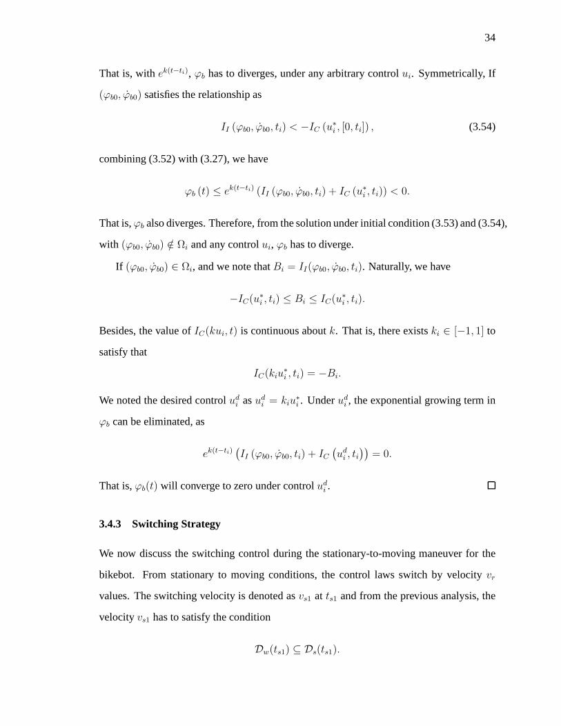
34

That is, withek(t−ti), ϕb has to diverges, under any arbitrary controlui. Symmetrically, If

(ϕb0, ϕb0) satisfies the relationship as

II (ϕb0, ϕb0, ti) < −IC (u∗i , [0, ti]) , (3.54)

combining (3.52) with (3.27), we have

ϕb (t) ≤ ek(t−ti) (II (ϕb0, ϕb0, ti) + IC (u∗i , ti)) < 0.

That is,ϕb also diverges. Therefore, from the solution under initial condition (3.53) and (3.54),

with (ϕb0, ϕb0) /∈ Ωi and any controlui, ϕb has to diverge.

If (ϕb0, ϕb0) ∈ Ωi, and we note thatBi = II(ϕb0, ϕb0, ti). Naturally, we have

−IC(u∗i , ti) ≤ Bi ≤ IC(u∗i , ti).

Besides, the value ofIC(kui, t) is continuous aboutk. That is, there existski ∈ [−1, 1] to

satisfy that

IC(kiu∗i , ti) = −Bi.

We noted the desired controludi asudi = kiu∗i . Underudi , the exponential growing term in

ϕb can be eliminated, as

ek(t−ti)(II (ϕb0, ϕb0, ti) + IC

(udi , ti

))= 0.

That is,ϕb(t) will converge to zero under controludi .

3.4.3 Switching Strategy

We now discuss the switching control during the stationary-to-moving maneuver for the

bikebot. From stationary to moving conditions, the controllaws switch by velocityvr

values. The switching velocity is denoted asvs1 at ts1 and from the previous analysis, the

velocityvs1 has to satisfy the condition

Dw(ts1) ⊆ Ds(ts1).

35

-2.5 -2 -1.5 -1 -0.5 0 0.5 1 1.5 2 2.5-10

-5

0

5

10Exp

Desired

ϕb (deg)

ϕb

(deg

/s)

(a)

-60 -40 -20 0 20 40 60-200

-100

0

100

200Controlled

Desired

ϕw (deg)

ϕw

(deg

/s)

(b)

100 120 140

-2

-1

0

1

2

ϕb

(deg

)

Time (s)

(c)

100 120 140-60

-40

-20

0

20

40

60

ϕw

(deg

)

Time (s)

(d)

Figure 3.1: Gyro-balancer orbital regulation results. (a)Bikebot rolling trajectory onϕb-ϕbphase plan. (b) Flywheel pivoting trajectory onϕw-ϕw phase plan. (c) Bikebot roll angleϕb trajectory. (d) Flywheel pivoting angleϕw trajectory.

To switch the control fromus (under the steering balance) touw (under the gyro-balancer),

that is, from moving-to-stationary transition, we consider the switching velocity atvs2 with

time ts2. The condition that needs to be satisfied is given as(ϕb(ts2), ϕb(ts2)) ∈ Dw. In

this case, the gyro-balancer controller can balance the system with a zero steering angleφ.

However, in practice, this condition is difficult to satisfyunder zero steering angle, partic-

ularly under possibly disturbances. We will present experimental results and discussion in

the next section.

3.5 Experiments results

We first demonstrate the stationary balance control performance under the orbital stabiliza-

tion controluw. The values of the major bikebot parameters aremb = 37.5 kg, hb = 0.64

36

-3 -2 -1 0 1 2 3-0.8

-0.6

-0.4

-0.2

0

0.2

0.4

0.6

0.8

ϕb (deg)

ϕb

(deg

/s)

(a)

-3 -2 -1 0 1 2 3

-6

-4

-2

0

2

4

6

ϕb (deg)

ϕb

(deg

/s)

(b)

-4 -3 -2 -1 0 1 2 3 4-40

-20

0

20

40

ϕb (deg)

ϕb

(deg

/s)

(c)

Figure 3.2: The DOA plots of the gyro-balancer and steering balance controls. (a) TheDOA plots under gyro-balancer orbital regulation controluw with initial conditionϕw0 = 0and various parameters. Blue:mb = 55 kg,ωs = 1500 rpm,hb = 0.64 m; Green:mb = 42kg,ωs = 1500 rpm,hb = 0.64 m; Red:mb = 55 kg,ωs = 1200 rpm,hb = 0.64 m; Black:mb = 55 kg,ωs = 1200 rpm,hb = 0.48 m. (b) The DOA plots of the gyro-balancer controluw and steering controlus. (c) Plots ofΩw andΩs. Blue: boundary ofΩw atmb = 55kg andωs = 1500 rpm; Green, red and black: boundaries ofΩs undervr = 0.75 m/s,vr = 1.00 m/s andvr = 1.50 m/s.

m andωs = 1500 rpm. Figs. 3.1(a) and 3.1(b) show the phase portraits of theϕb-ϕb and

ϕw-ϕw, while Figs. 3.1(c) and 3.1(d) show the roll angleϕb and pivoting angleϕw profiles.

The desired roll angle orbits reach to±2 deg. The bikebot is released atϕb0 = −1.2 deg

andϕb0 = 0 deg/s withϕw0 = 0. From Fig. 3.1(c), after several periods, the bike roll angle

profiles converge to the desired roll orbitOb. This is clearly shown in Fig. 3.1(a). When

the rolling motion reaches the desired orbit, the flywheel pivoting motion is also near the

pivoting orbit, as shown in Fig. 3.1(b). The flywheel pitching trajectory is within the range

of ±50 deg as shown in Fig. 3.1(d).

37

70 75 80 85 90 95 100 105 110 115-2

-1

0

1

2

84 86 88 90 92 94 96 98 100 102 104-0.5

0

0.5

1

ϕb

(deg

)ϕb,ϕbe

(deg

)

Time (s)(a)

-50

0

50

70 75 80 85 90 95 100 105 110 115-5

-3

-1

1

3

56

ϕw

(deg

)φ

(deg

)

Time (s)(b)

0 10 20 30 40 50-1

-0.8

-0.6

-0.4

-0.2

0

0.2

0.4

0.6

0.8

1

Gyro-balancerSteeringTrackingTarget

X (m)

Y(m

)

(c)

70 75 80 85 90 95 100 105 110 115

0

1

2

8 10 12 14 16 18 20 22 24 26 280

0.2

0.4

vr

(m/s

)X (m)

Time (s)

eP

(m)

(d)

-2 -1.5 -1 -0.5 0 0.5 1 1.5 2

-10

-5

0

5

10

g boundary

successfailure 1failure 2

ϕb (deg)

ϕb

(deg

/s) Ωw

(e)

-0.05 0 0.05 0.1 0.15-0.1

-0.05

0

0.05

0.1

successfailure 1failure 2II+I

D=I

C

II (rad)

I D(r

ad)

ID + II < IC

ID + II > IC

(f)

Figure 3.3: Switched balance control results. (a) Bikebot roll angleϕb and target roll angleϕbe. (Top-figure: blue and red curves underuw and green curve underus; Bottom-figure:blue and red curves are the roll angleϕb(t) and the desiredϕbe(t), respectively. The solidand dash lines portion represent the only balancing and balancing-tracking,respectively. (b)Flywheel pivoting angleϕw and steering angleφ. Blue and red portion underuw controland the green portion underus control.) (c) Bikebot planar position(X, Y ). Purple dash,blue solid, and black square portions are underuw, us, and EIC-based velocity-steeringcontrol (uv, us), respectively. The red dash line is the target path. (d) Bikebot velocityvrand path following erroreP . For the top-figure, blue and red portion are underuw anduscontrols, respectively. (e) State variable(ϕb(ts2), ϕb(ts2)) on theϕb-ϕb plane. Blue squares,red circles, red crosses marks are for the success, failure with |II + ID| ≤ IC , failure with|II + ID| > IC cases, respectively. The black lines are the boundary ofΩw. (f) Runningconditions in theII-ID plane. Blue squares, red circles, and red crosses are for thesuccess,failure with |II + ID| ≤ IC , failure with |II + ID| > IC cases, respectively. The black linerepresentsII + ID = IC .

38

Fig. 3.2(a) shows the sets boundaries ofDw at various combinations of parametermb,

hb andωs. From these plots, we observe that the smallerms, smallerhb, or largerωs

values, the DOA estimatesDw become larger. Under the outdoor experiment condition

(i.e.,mb = 55 kg, hb = 0.64 m andωw = 1500 rpm, the blue curve in Fig. 3.2(a)), the

estimated maximum controllable roll angle by gyro-balancer control uw is less than 1.7

deg. That region is also plotted in Fig. 3.2(b) and is boundedby blue curve. If the initial

roll states(ϕb0, ϕb0) ∈ Dw, controlleruw can drive the state to converge to orbitOb (i.e.,

red circle). Fig. 3.2(b) also shows the plot ofDs under different velocityvr values. For

vr = 0.85 (black solid lines) and1 m/s (black dash lines), the regionsDs increases in

size. If vr ≥ 0.85 m/s, DOA regionDw underuw is covered byDs underus. Fig. 3.2(c)

shows the boundaries of largest DOAsΩs andΩw under various velocity values. With

increasedvr, regionΩs is enlarged. Whenvr ≥ 0.75 m/s,Ωw ⊂ Ωs. Comparing withDs

in Fig. 3.2(b), for a givenvr, Ωs is almost at the same size as that ofDs.

We also run stationary-to-moving-to-stationary experiments under the switching con-

trol betweenuw andus. During the second moving phase, the bikebot is commanded to

track a straight-line trajectory under the EIC-based steering controlus, and the first and

third transition phases, balancing is the only target underuw. Fig. 3.3 shows the perfor-

mance of one experimental run results. The stationary-to-moving transition are from 66.2

s to 81.6 s and the moving-to-stationary duration is from 106.3 s to 118.5 s. The path

following portion is therefore from 86.1 s to 95.5 s. The balanced roll angle profiles are

plotted in Fig. 3.3(a). In the first and third portions, the bikebot experiences the periodical

swing motions in the range about[−1, 1] deg under the orbital stabilization controluw. In

the middle portion, under steering controlus, roll angle is within the range of[−1, 1] deg.

Moreover, the roll angle tracks the desired trajectoryϕbe(t) by the EIC design. The gyro-

balancer pivoting and steering angle control inputs are shown in Fig. 3.3(b). Fig. 3.3(c)

shows the bikebot planar position and the position errors are held within±0.4m as shown

in Fig. 3.3(d). The switching velocities are designed atvs1 = 1.2 m/s andvs2 = 1.9 m/s

andvs1 satisfies the DOA analysis.

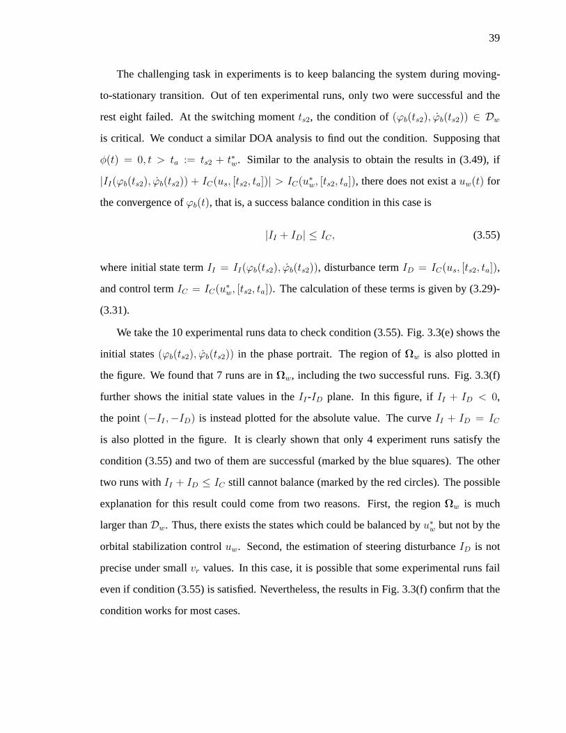
39

The challenging task in experiments is to keep balancing thesystem during moving-

to-stationary transition. Out of ten experimental runs, only two were successful and the

rest eight failed. At the switching momentts2, the condition of(ϕb(ts2), ϕb(ts2)) ∈ Dw

is critical. We conduct a similar DOA analysis to find out the condition. Supposing that

φ(t) = 0, t > ta := ts2 + t∗w. Similar to the analysis to obtain the results in (3.49), if

|II(ϕb(ts2), ϕb(ts2)) + IC(us, [ts2, ta])| > IC(u∗w, [ts2, ta]), there does not exist auw(t) for

the convergence ofϕb(t), that is, a success balance condition in this case is

|II + ID| ≤ IC , (3.55)

where initial state termII = II(ϕb(ts2), ϕb(ts2)), disturbance termID = IC(us, [ts2, ta]),

and control termIC = IC(u∗w, [ts2, ta]). The calculation of these terms is given by (3.29)-

(3.31).

We take the 10 experimental runs data to check condition (3.55). Fig. 3.3(e) shows the

initial states(ϕb(ts2), ϕb(ts2)) in the phase portrait. The region ofΩw is also plotted in

the figure. We found that 7 runs are inΩw, including the two successful runs. Fig. 3.3(f)

further shows the initial state values in theII-ID plane. In this figure, ifII + ID < 0,

the point(−II ,−ID) is instead plotted for the absolute value. The curveII + ID = IC

is also plotted in the figure. It is clearly shown that only 4 experiment runs satisfy the

condition (3.55) and two of them are successful (marked by the blue squares). The other

two runs withII + ID ≤ IC still cannot balance (marked by the red circles). The possible

explanation for this result could come from two reasons. First, the regionΩw is much

larger thanDw. Thus, there exists the states which could be balanced byu∗w but not by the

orbital stabilization controluw. Second, the estimation of steering disturbanceID is not

precise under smallvr values. In this case, it is possible that some experimental runs fail

even if condition (3.55) is satisfied. Nevertheless, the results in Fig. 3.3(f) confirm that the

condition works for most cases.

40

3.6 Conclusion

This chapter presented a stationary balance control law, a moving balance control law,

and an integrated balance control of autonomous bikebot system in complete stationary-

to-moving maneuvers. Gyro-balance and steering actuationare two main effective con-

trol strategies for stationary and moving cases respectively. We analyzed the DOA of the

closed-loop systems under these two control designs and then built on the DOA analysis,

a safety control strategy was designed for stationary-to-moving maneuvers. We conducted

extensive experiments to illustrate and demonstrate the analysis and design. The results

validated the effectiveness of the switching control strategies.

From theoretical analysis and experiments results, the proposed switching control seems

not robust enough for handling large disturbances in practical experiments. We plan to re-

lax some assumptions in the analysis and develop a combined gyro-balancer and steering

control strategy to enhance the balance performance in future.

41

Chapter 4

Bikebot Autonomous Tracking Control

4.1 Introduction

Underactuated balancing systems such as bicycles or motorcycles provide a unique plat-

form to train and treat human with postural balance disabilities [38,59]. Balancing control

of the bikebot is presented in Chapter 3. To further understand and tune the characteristics

of human balance motor skills in these unstable physical human-robot interactions, it is

desirable to design and build an autonomous trajectory tracking and balancing capability

for the bikebot system.

Trajectory tracking control of a riderless autonomous bicycle (or motorcycle) has also

been proposed and studied in [11, 13, 17, 41–43, 60]. Steering and velocity control are

the main two actuations for the autonomous bicycles or motorcycles designs except that

in [17,60], additional mechanisms such as weight-shiftingare used to assist the balance of

the systems. Although many above-mentioned research work discuss the motion control of

autonomous bicycles, few experimental results and demonstration have been reported. The

results of the Blue team in the 2005 DARPA Challenge confirm the difficulties to achieve

accurately trajectory tracking and balance control of autonomous single-track vehicles [13].

One of the research goals of this chapter is to demonstrate the experiments of trajectory

tracking and balancing of autonomous bikebot using steering and velocity control.

Understanding the human sensorimotor mechanism in the physical unstable rider-bicycle

interaction is studied in recent work in [12, 29, 30]. Modeling and pose estimation of the

rider-bicycle interactions are reported in [26, 27, 61]. Tofurther identify the human con-

trol strategies quantitatively, the research work in [21, 22] present the human upper-body

42

movement and steering control models and their influences onplatform balance. Bikebot

is utilized in the work presented in [21, 22]. The use of the gyro-balancer as an additional

actuation helps the balance of the stationary bikebot [20] and also enables the further tun-

ing of human motor skills through the physical rider-bikebot interactions. Another goal of

this work is to integrate the gyro-balancer design into the trajectory-tracking and balancing

control.

In this chapter, a trajectory tracking and balance control law is first presented. With the

steering and velocity control, the bikebot can track a target trajectory autonomously. The

controller design is built on an extension of the EIC structure of the nonlinear dynamics of

the bikebot system [11,41]. The EIC-based control is modified and implemented to achieve

both trajectory-tracking and platform-balancing tasks. The control design is then extended

by incorporating the gyro-balancer actuation to further enhance the control performance.

The use of additional gyro-balancer torque further reducesthe position tracking error and

the performance improvement is also guaranteed by design. The control systems designs

are validated and demonstrated by experiments.

To our best knowledge, there is no reported experimental demonstration for the precise

and successful trajectory tracking and balance control of autonomous bicycles or motor-

cycles. The experiments in [42, 62] and other demonstrations only show the balance ca-

pability of controlled bicycle or motorcycle systems and trajectory tracking is not among

the control tasks. Indeed, from control systems design viewpoint, trajectory tracking and

platform balancing are two competing tasks. Other studies (e.g., [11,17,43]) do not include

experimental demonstration and validation. The EIC-basedcontrol with inclusion of the

gyro-balancer design complements the human rider control strategies developed in litera-

ture [21, 22, 29, 30]. The control design in this chapter alsoenables the use of bikebot for

control of physical human-robot interactions. Although the chapter focuses on the bikebot,

the proposed control systems approach can be applied to other underactuated balancing

systems, such as pole-cart, Furuta pendulum, or biped walkers, etc.

The remainder of this chapter is organized as follows. The control laws are designed

43

in Section 4.2. The theoretical analysis for this control system stability and performance is

demonstrated in Section 4.3. The designed experiments are presented in Section 4.4. The

concluding remarks are discussed in Section 4.5.

4.2 EIC-based controller design

The bikebot dynamics in (2.9) and (2.12) can be converted into an nearly EIC form. The

nearly EIC form of a nonlinear dynamical system is an extension of the EIC form intro-

duced in [11].

Definition 4.1. Ann(= m+p)-dimensional nonlinear control system is called in annearly

external/internal convertible formif the system is of the form

Σ :

xi = xi+1, xm = u, i = 1, · · · , m− 1,

αj = αj+1,

αp = f(x,α) + g(x,α)u+ gi(x,α)ui,

y = x1, j = 1, · · · , p− 1,

(4.1)

with inputsu, ui ∈ R, outputy ∈ R, state variables(x,α), with x = [x1 · · · xm]T ∈ Rm

and α = [α1 · · · αp]T ∈ Rp. Functionsf(x,α), g(x,α) and gi(x,α) are smooth and

g(x,α) 6= 0 for all (x, α) ∈ Br ⊂ Rn+p is an open ball. Moreover, we refer to theexternal

subsystemof Σ as

Σext : xi = xi+1, xm = u, i = 1, · · · , m− 1, (4.2)

and theinternal subsystemof Σ as

Σint : αi = αi+1, αp = f(x,α) + g(x,α)u+ gi(x,α)ui, (4.3)

for i = 1, · · · , p− 1.

Fig. 4.1 shows the structure of the nearly EIC system. The nearly EIC systemΣ is

convertiblebecauseΣint is nearly converted toΣext (with an addition internal controlui

44

x1x2xm

α1α2αp

u

ui

∫

∫∫

∫

∫

∫ y

f(x,α)+g(x,α)u+gi(x,α)ui

Internal subsystem

External subsystem

Figure 4.1: A nearly external/internal convertible system.

term), andΣext is nearly converted toΣint (again with an addition internal controlui term)

under a simple transformationu = g(x,α)−1 [v − f(x,α)]. To see this dual-structure

property, definingξ = α1 as the dual output and applying the above transformation to

Σ (4.1), we obtain thedualof Σ(u).

Σd :

xi = xi+1, xm = −g−1(x,α)f(x,α) + g−1(x,α)v,

αj = αj+1, αp = v + g−1(x,α)gi(x,α)ui,

ξ = α1, i = 1, · · · , m− 1, j = 1, · · · , p− 1.

(4.4)

The bikebot rolling dynamics (2.9) can be rewritten as

Jtϕb = f(ϕb) + gψ(ϕb)uψ + gwuw, (4.5)

with Jt = mbh2b + Jb + Iz(1 + s2

ϕw)/2, f(ϕb) = −mbhb cϕb vrψ + mbh2b cϕb sϕb ψ

2 +

mbhbg sϕb +Iz cϕw sϕb ψ(ωs− ϕb sϕw /2− ψ cϕb cϕw /2) +mbgltlb tan φ cξ cϕb

l, gw = −Iz(ωs−

ϕ sϕw /2− ψ cϕb cϕw /2) cϕw , andgψ(ϕb) = −mbhblb cϕb. The equivalent control inputs for

rolling areuψ anduw = ϕw. Combining with (2.12) and (4.5), the EIC form of this system

is

Σext : r(3)C2

= uN , (4.6a)

Σint : ϕ = J−1t [f(ϕb) + gψ(ϕb)uψ + gwuw] . (4.6b)

45

For a given desired trajectoryT :(Xd(t), Yd(t)), we design a linear feedback controller

for Σext [22]

uextN = r

(3)d − b2ep − b1ep − b0ep, (4.7)

anduext = R−1ψ (Ψ + uext

N ), whererd = [Xd(t), Yd(t)]T , errorep(t) = [eX , eY ]T = rC2 −

rd, andr(3)d denotes the third derivative ofrd. The control gainsbi, i = 0, 1, 2, are chosen

to guarantee thats3 + b2s2 + b1s+ b0 = 0 is Hurwitz. Under (4.7), the external vector field

Next is defined as

Next :=

X (t)

X (t)

X(3)d − Σ2

i=0bie(i)X

Y (t)

Y (t)

Y(3)d − Σ2

i=0bie(i)Y

. (4.8)

Using control design (4.7), the BEM is defined as

E =

(x, ϕbe)∣∣∣ϕb = ϕbe(ψ, vr,u

ext, ϕw

)

, ϕb = ϕb = 0

, (4.9)

wherex = [rTC2rTC2

rTC2]T andα = [ϕb ϕb]

T . In (4.9), the roll angle equilibriumϕbe =

ϕbe(ψ, vr,uext, ϕw) is the solution of the following equation (underuψ = uext

ψ anduw = 0)

F (ϕbe, ψ, vr,u, ϕw) = f(ϕb) + gψ(ϕb)uextψ = 0. (4.10)

The derivativesϕbe andϕbe can be approximated by the directional derivatives alongNext

with uw = 0 as

LNextϕbe = LNext

ϕe +∂ϕbe∂t

, L2Next

ϕbe = LNextLNext

ϕbe.

If the gyro-balancer is not actuated, that is,uw = 0, the internal system controller is

designed as

uintψ = g−1

ψ (ϕb)(−f(ϕb) + Jtvintψ ) (4.11)

where

vintψ = L2

Nextϕbe − a1eϕb − a0eϕb (4.12)

46

with the tracking errors definitionseϕb = ϕb − ϕbe, eϕb = ϕb − ϕbe ≈ ϕb − LNextϕbe, and

a0, a1 > 0. Under thisuintψ , the closed-loop error dynamics forΣint is eϕ + a1eϕ + a0eϕ =

0 and asymptotically stable. Therefore, without using the gyro-balancer actuation, the

controller is

C : ur = uextr , uψ = uint

ψ , uw = 0. (4.13)

The gyro-balancer pivoting controluw and the modifieduintψ are designed in the follow-

ing. According to the EIC control structure, under control input uext = [uextr uext

ψ ]T , the

bikebot position(X(t), Y (t)) converges to the desired trajectoryT exponentially. How-

ever, for the balancing task, the steering inputuintψ is different fromuext

ψ and thus introduces

position tracking errorsep. On the other hand,uintψ has to tune roll angleϕb to follow equi-

librium ϕbe. The goal of the gyro-balancer controluw is to assist platform balancing under

uintψ . We consider that under the combineduw anduint

ψ , the balancing capability is the same

asuintψ in (4.11) and thus

Jtvintψ = f(ϕb) + gψ(ϕb)u

intψ = f(ϕb) + gψ(ϕb)u

intψ + gwuw. (4.14)

Underuext (4.7) anduext = R−1ψ (Ψ + uext

N ), the position tracking closed-loop dynam-

ics is

r(3)d − b2ep − b1ep − b0ep = Ψ + Rψ

uextr

uextψ

. (4.15)

On the other hand, from (4.6a) and control (4.7),

r(3)c = Ψ + Rψ

uextr

uintψ

(4.16)

and subtracting (4.15) from (4.16), the real closed loop tracking system is

e(3)p + b2ep + b1ep + b0ep = dp := Rψ

0

uintψ − uext

ψ

. (4.17)

Using the BEM definition (4.9),uextψ can be rewritten in terms ofϕbe as

uextψ = −g−1

ψ (ϕbe)f(ϕbe). (4.18)

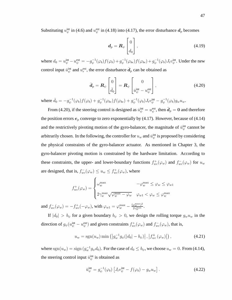
47

Substitutinguintψ in (4.6) anduext

ψ in (4.18) into (4.17), the error disturbancedp becomes

dp = Rψ

0

d0

, (4.19)

whered0 = uintψ −uext

ψ = −g−1ψ (ϕb)f(ϕb)+g−1

ψ (ϕbe)f(ϕbe)+g−1ψ (ϕb)Jtv

intψ . Under the new

control inputuintψ anduext

r , the error disturbancedp can be obtained as

dp = Rψ

0

d0

= Rψ

0

uintψ − uext

ψ

, (4.20)

whered0 = −g−1ψ (ϕb)f(ϕb) + g−1

ψ (ϕbe)f(ϕbe) + g−1ψ (ϕb)Jtv

intψ − g−1

ψ (ϕb)gwuw.

From (4.20), if the steering control is designed asuintψ = uext

ψ , thendp = 0 and therefore

the position errorsep converge to zero exponentially by (4.17). However, becauseof (4.14)

and the restrictively pivoting motion of the gyro-balancer, the magnitude ofuintψ cannot be

arbitrarily chosen. In the following, the controller foruw anduintψ is proposed by considering

the physical constraints of the gyro-balancer actuator. Asmentioned in Chapter 3, the

gyro-balancer pivoting motion is constrained by the hardware limitation. According to

these constraints, the upper- and lower-boundary functions f+wc(ϕw) andf−

wc(ϕw) for uw

are designed, that is,f−wc(ϕw) ≤ uw ≤ f+

wc(ϕw), where

f+wc(ϕw) =

ωmaxw −ϕmax

w ≤ ϕw ≤ ϕw1

2γmaxw

√ϕmaxw − ϕw ϕw1 < ϕw ≤ ϕmax

w

andf−wc(ϕw) = −f+

wc(−ϕw), with ϕw1 = ϕmaxw − (ωmax

w )2

2γmaxw

.

If |d0| > bψ for a given boundarybψ > 0, we design the rolling torquegwuw in the

direction ofgψ(uintψ − uext

ψ ) and given constraintsf+wc(ϕw) andf−

wc(ϕw), that is,

uw = sgn(uw) min(∣∣g−1w gψ(|d0| − bψ)

∣∣ ,∣∣f±wc (ϕw)

∣∣), (4.21)

wheresgn(uw) = sign (g−1w gψd0). For the case ofd0 ≤ bψ, we chooseuw = 0. From (4.14),

the steering control inputuintψ is obtained as

uintψ = g−1

ψ (ϕb)[Jtv

intψ − f(ϕb) − gwuw

]. (4.22)

48

Remark 4.1. Because of physical limitation of the gyro-balancer pivoting effects, the bal-

ancing actuationuw itself might not be powerful enough to fully balance the platform. That

is the main reason why utilizinguw as an auxiliary control when|d0| is large. A practi-

cal scenario is that the desired trajectory has a sharp turning or the balancing platform

faces strong disturbances in a short time interval. Becauseof the limited actuation, in most

parts of the tracking process, the balancing performance mainly depends on the steering

actuation.

4.3 Stability analysis

Under the EIC-based controlC : (uextr , u

intψ , 0), the position tracking error is denoted asep.

With the additional gyro-balancer actuation, the control inputs and the position tracking

error are denoted asC : (uextr , u

intψ , uw) andep, respectively. It can be shown that under the

new controlC, the magnitude of the tracking errors is reduced. To show this property, the

following results are first demonstrated.

Property 4.1. The magnitude of error disturbancedp under controllerC is not greater than

that ofdp under controllerC.

Proof. From (4.19) and (4.20), this property is equivalent to show|d0| ≤ |d0|. For the case

of |d0| < bψ, uw = 0 is utilized, thus|d0| = |d0|. Therefore∥∥dp∥∥

2= ‖dp‖2. For the case

|d0| > |d0|, we have

d0 − d0 = uintψ − uint

ψ = g−1ψ (ϕ)gwuw. (4.23)

Form the sign and amplitude definition ofuw, we conclude the following relationships:

sgn (d0) = sgn(g−1ψ gwuw

)and |g−1

ψ gwuw| ≤ |d0| − bψ < |d0|. Therefore, under taking

the absolute value of (4.23) without changing the form, the relationship|d0| − |d0| =

|g−1ψ gwuw| > 0 is obtained.

Under controllerC, the EIC structure and property are still held. Therefore, as shown

in [11, 22], the closed-loop errorsep andep asymptotically converge to a bounded region

49

near origin. Similar to (4.17), the obtained dynamics forep is

e(3)p + b2¨ep + b1 ˙ep + b0ep = dp. (4.24)

Definingex = [eTp , eTp , e

Tp ]T andeϕb = [eϕb , eϕb]

T , similar to [11], the magnitudes of the

disturbancesdp anddp are assumed to be affine function ofex andex, respectively,

‖dp‖2 ≤ k0 + k1 ‖ex‖2 ,∥∥dp∥∥

2≤ k0 + k1 ‖ex‖2 , (4.25)

whereex = [eTp , ˙eTp , ¨e

Tp ]T andk0, k1, k0, k1 > 0 are positive constants. Because of the

results in Property 4.1, it is assumed that

k0 ≤ k0, k1 ≤ k1. (4.26)

The following results about errorsep andep are based on the following property.

Property 4.2. Under controllersC and C, the position tracking errorsep(t) and ep(t)

exponentially converge to regions near the origin. Moreover, there exist error boundsebp(t)

and ebp(t), that is,‖ep(t)‖ ≤ ebp(t) and‖ep(t)‖ ≤ ebp(t), thenebp(t) ≤ ebp(t), for ∀t ≥ 0.

Proof. We prove the property through the Lyapunov stability theorem [58] and the results

by Property 4.1. Using state variableex, we re-write the error dynamics (4.17) as

ex = Aex + dp,A = A0 ⊗ I2,A0 =

0 1 0

0 0 1

−b0 −b1 −b2

, (4.27)

where operator⊗ represents the Kronecker product andIn ∈ Rn×n is then-dimensional

identity matrix.

The Lyapunov functionV = eTxPex is introduced, where positive definition matrix

P = P T ∈ R6×6 is the solution of Lyapunov equationATP + PA = −I6. Note that

P always exists sinceA is Hurwitz. Following the stability of the perturbed systems [58]

and (4.25), the time derivative ofV = eTxPex is

V ≤ −(

1

c2− k1

2c2c1

)

V + 2c2k0

√

V

c1, (4.28)

50

wherec1 = λmin(P ) > 0 andc2 = λmax(P ) > 0 are the minimum and maximum eigen-

values ofP , respectively. DefiningW =√V , we write (4.28) as

W ≤ −αW +2c2k0√c1, (4.29)

whereα = 12

(1c2− k1

2c2c1

)

> 0, namely,k1 < c12c22

. ConsideringW (t) =√

V (t) ≥√c1‖ex(t)‖ and by comparison lemma [58], from (4.29) it is obtained that

‖ex(t)‖ ≤ cre−αt‖e(0)‖ +

2c2rk0

α=: ebp(t), (4.30)

wherecr = c2/c1. For the error dynamics under controllerC, the inequality is obtained as

‖ex(t)‖ ≤ cre−αt‖e(0)‖ +

2c2rk0

α=: ebp(t), (4.31)

with α = 12

(1c2− k1

2c2c1

)

> 0 andk1 <c12c22

. From (4.30) and (4.31), it is straightforward

to obtain that both errors exponentially converge to the regions near the origin with bounds

2c2rk0α

and 2c2r k0α

, respectively. Considering‖ex(0)‖ = ‖ex(0)‖ and α ≥ α, e−αt ≤ e−αt

for any t and k0α

≤ k0α

, and thusebp(t) ≤ ebp(t) for any t ≥ 0 because of relationships

in (4.26).

From (4.14), underC, the balancing control effect is the same as that ofC. The internal

system closed-loop error dynamics is still as

eϕb + a1eϕb + a0eϕb = dϕb, (4.32)

where disturbancedϕb = ϕbe − L2Nextϕbe + a1

(ϕbe − LNextϕbe

)is also bounded by the

norms of the desired trajectory,ep andeϕb [11]. Because of the unchanged internal error

dynamics (4.32) underC andC, the stability and tracking performance for the BEM are the

same for these two controllers. Note that this property is obtained by the particular gyro-

balancer controluw given by (4.14). Other alternative control ofuw can be also designed

to achieve different properties and to obtain the performance trade-off between position

tracking errorex and balancing erroreϕb .

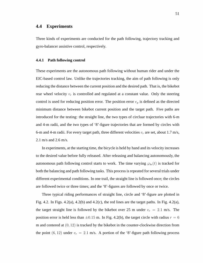
51

4.4 Experiments

Three kinds of experiments are conducted for the path following, trajectory tracking and

gyro-balancer assistive control, respectively.

4.4.1 Path following control

These experiments are the autonomous path following without human rider and under the

EIC-based control law. Unlike the trajectories tracking, the aim of path following is only

reducing the distance between the current position and the desired path. That is, the bikebot

rear wheel velocityvr is controlled and regulated at a constant value. Only the steering

control is used for reducing position error. The position error ep is defined as the directed

minimum distance between bikebot current position and the target path. Five paths are

introduced for the testing: the straight line, the two typesof circluar trajectories with 6-m

and 4-m radii, and the two types of ‘8’-figure trajectories that are formed by circles with

6-m and 4-m radii. For every target path, three different velocitiesvr are set, about 1.7 m/s,

2.1 m/s and 2.6 m/s.

In experiments, at the starting time, the bicycle is held by hand and its velocity increases

to the desired value before fully released. After releasingand balancing autonomously, the

autonomous path following control starts to work. The time varyingϕbe(t) is tracked for

both the balancing and path following tasks. This process isrepeated for several trials under

different experimental conditions. In one trail, the straight line is followed once; the circles

are followed twice or three times; and the ‘8’-figures are followed by once or twice.

Three typical riding performances of straight line, circleand ‘8’-figure are plotted in

Fig. 4.2. In Figs. 4.2(a), 4.2(b) and 4.2(c), the red lines are the target paths. In Fig. 4.2(a),

the target straight line is followed by the bikebot over 25 m undervr = 2.1 m/s. The

position error is held less than±0.15 m. In Fig. 4.2(b), the target circle with radiusr = 6

m and centered at(0, 12) is tracked by the bikebot in the counter-clockwise direction from

the point(6, 12) undervr = 2.1 m/s. A portion of the ‘8’-figure path following process

52

10 15 20 25 30 355.8

5.9

6

6.1

X (m)

Y(m

)

(a)

−6 −4 −2 0 2 4 6

6

8

10

12

14

16

18

X (m)

Y(m

)

(b)

−5 0 5 10 15 20

6

8

10

12

14

16

18

X (m)

Y(m

)

(c)

10 15 20 25 30 35−0.5

0

0.5

1

1.5

S (m)

ϕb

(deg

)

(d)

0 50 100 150 200 250 300 350

−5

−4

−3

−2

θP (deg)

ϕb

(deg

)

(e)

0 100 200 300 400 500 600 700

−6

0

6

−4

−2

2

4

88

−8

θP (deg)

ϕb

(deg

)

(f)

Figure 4.2: Bikebot path following results. (a), (b) and (c)Horizontal position results ofStraight line, circle and ‘8’-figure. (Blue lines are the bikebot horizontal position, Red linesare the target paths.) (d), (e) and (f) Roll angle tracking results of Straight line, circle and‘8’-figure. (Blue lines are the measured bikebot roll angleϕb, Red lines are the targetϕbetrajectories.)

is also plotted in Fig. 4.2(c). The target path includes two circles with a 6-m radius and

centered at(0, 12) and(12, 12), respectively. Undervr = 2.1 m/s, the bikebot starts near the

circle-connection point(6, 12), and follows the entire left circle in the counter-clockwise

direction and then the entire right circle in the clockwise direction. The blue line is the

actual position trajectory. The roll angleϕbe tracking results in these three processes are

also included in Fig. 4.2. From straight line to ‘8’-figure, the target path becomes complex,

and the position error also increases.

In Figs. 4.2(d), 4.2(e), and 4.2(f), the roll angle trajectories are displayed along the path

53

arc-lengthS(t) rather than time. For the straight line, theX-coordinate of the position is

used to represent the arc-length. For the circle and ‘8’-figure, the angular positionθP is used

to represent the arc-length. Angleθp is calculated from the vector direction from centers

of the circles to the current position. Thus, for the circle path, an entire circle corresponds

to θp ∈ [0, 360] deg, the ‘8’-figureθp ∈ [0, 720] deg, with the second circleθp ∈ [360, 720]

deg. From Fig. 4.2, the actual roll angleϕb (blue line) can track the desiredϕbe (red line)

closely.ϕb of the circle following is shown in Fig. 4.2(e). The most challenging case for

roll angle following is for the ‘8’-figure trajectory, whichcan be considered as following

two circles sequentially from two opposite directions. As shown in Fig. 4.2(f), after passing

the connection point(6, 12) (i.e.,θp = 360 deg),ϕbe experiences a dramatic change from a

negative to positive value.

Fig. 4.2 only demonstrates some examples out of all experiments under different riding

conditions. Statistical analysis is required in order to reveal the performance differences

among conditions. As previously mentioned, 15 experimental conditions (5 different paths

and 3 different velocities) were conducted. Under each condition, 4 completed trails (simi-

lar as Fig. 4.2) are gathered. In every single process, the average of absolute position error

|ep|ave and balancing error|eα|ave are calculated. For every riding condition, the mean val-

ues and standard derivations of|ep|ave and |eα|ave are calculated and shown in Table 4.1.

‘S’, ‘C6’, ‘C4’, ‘E6’ and ‘E4’ represent the straight line, circle with 6m radius, circle with

4m radius, ‘8’-figure with 6m radius and ‘8’-figure with 4m radius, respectively. ‘L’, ‘M’

and ‘H’ means the low, middle and high bikebot velocityvr, respectively.

Table 4.1: The mean and standard deviation of|ep|ave(m) and |eα|ave(deg) for the pathfollowing performances.

Path |ep|ave(L) |eα|ave(L) |ep|ave(M) |eα|ave(M) |ep|ave(H) |eα|ave(H)S 0.13±0.03 0.28±0.02 0.11±0.05 0.22±0.02 0.18±0.04 0.34±0.03

C6 0.28±0.04 0.54±0.03 0.31±0.04 0.38±0.03 0.39±0.05 0.48±0.03C4 0.35±0.05 0.81±0.02 0.37±0.06 0.82±0.05 0.43±0.10 1.09±0.09E6 0.33±0.10 0.61±0.06 0.38±0.10 0.73±0.08 0.49±0.11 0.84±0.11E4 0.41±0.13 0.98±0.06 0.56±0.25 1.45±0.14 0.69±0.30 1.75±0.17

54

From Table 4.1, under the same velocity, the results of the straight line following always

have the smallest position error and tracking errors. The circles’ results are better than those

of ‘8’-figures’ trajectories. The results of big radius paths are better than those of the small

radius paths. When the velocity is increased, both the position errors and the balancing

tracking errors are enlarged. From the controller design, the path-following performance

is highly related to the roll angle tracking results. Ifϕb cannot converge toϕbe quickly,

the current position also cannot follow the target path in a short time. Due to the model

uncertainty, actuation errors and other factors, trackingthe near zeroϕbe(t) (Fig. 4.2(d))

is easier than tracking the non-zero target profiles (Fig. 4.2(e)). Compared to the fast and

dramatically changingϕbe(t) profile (Fig. 4.2(f)), the slow varyingϕbe(t) is easier to track.

4.4.2 Trajectory tracking control

We apply the EIC-based controller to track the moving point on the horizontal plane for the

bikebot system. The tracking erroreP is the distance between the bikebot and the target

moving point, aseP = (e2X + e2Y )0.5, whereeX , eY ∈ R are the errors in theX- andY -

directions, respectively. In the trajectory tracking control design, both the steer angleφ and

the velocityvr are considered as control inputs.

To improve the trajectory tracking performance, the regular EIC-based controller is

modified by a velocity vector design method [12]. In this experiment, both the regular

EIC-based controller and the enhanced EIC-based controller are tested for tracking the

same target trajectory. The performances of these two controller are compared. For this

comparison, the experimental conditions, the target trajectories and the control parameters

of these two controllers are the same. The only difference isthat the modified controller

has a new modified vector field in the external subsystem controller. A moving point on a

cosine wave is designed as the target with the time-parametrization,

xd (t) = 2t, yd (t) = −3 cos

(πt

3

)

+ 9.

55

0 10 20 30 40 508

10

12

14

16

TargetModifiedOriginal

X (m)

Y(m

)

(a)

0 10 20 30 40 500

0.2

0.4

0.6

0.8

1

ModifiedOriginal

X (m)

eP

(m)

(b)

10 20 30 40 50−1

−0.5

0

0.5

10 20 30 40 50−2

−1

0

1

ModifiedOriginal

ModifiedOriginal

X (m)

eX

(m)

eY

(m)

(c)

0 10 20 30 40 501.8

2

2.2

2.4

2.6

2.8

3

ModifiedOriginal

X (m)

vr

(m/s

)(d)

10 20 30 40 500.92

0.94

0.96

0.98

1

X (m)

τ(s−

1)

(e)

0 10 20 30 40 50−20

0

20

10

−10

0 10 20 30 40 50

−10

0

10

RealDesired

RealDesired

X (m)

ϕb

(deg

)ϕb

(deg

)

(f)

Figure 4.3: Tracking results comparison between the regular EIC controller and modifiedEIC controller. (a) Position trajectories. (black dash, blue solid and red solid lines arethe target trajectory, real trajectory under modified EIC control and real trajectory underregular EIC control.) (b) Position tracking error. (c) Position Tracking errors inX- andY -directions. (d) Bikebot real velocities under these two controllers. (e) time suspension ratein modified EIC control. (f) Roll angle tracking results. (Upper figure is for the modifiedEIC control, lower figure is for the original EIC control))

The results are shown in Fig. 4.3. From Fig. 4.3(a), both the enhanced EIC-based con-

troller and the regular one can track the target trajectory.The enhanced controller has better

performance than that under the regular EIC-based controller. The position tracking errors

are plotted in Fig. 4.3(b). After a few seconds from starting, the position tracking errors of

the enhanced controller are smaller than those of the regular control. The error elementeY

is reduced significantly in Fig. 4.3(c). In Fig. 4.3(d), besides the EIC controller, the velocity

56

vector field also changes the bikebot velocity. At the peak points of the target trajectory, the

velocity under enhanced controller is smaller than that of the regular one. In the modified

EIC control, the time coordinate of the target trajectory istuned according to the current

position errors, and the new time coordinateτ is introduced. The time suspension rateτ is

plotted in Fig. 4.3(e). In Fig. 4.3(f), the roll angleϕbe tracking results of these two test are

similar under these two controllers.

4.4.3 Gyro-balancer assistive control

In this experiment, the gyro-balancer control is used to enhance performance. A straight

line and a circular path are used as the desired paths for the bikebot to follow. Figs. 4.4, 4.5

and 4.6 show the straight line tracking experimental results under both controllersC andC.

The trajectory is designed such that the bikebot is controlled to track a straight-line with

a constant velocity. Figs. 4.4 and 4.5(a) show the tracking trajectories and tracking errors,

respectively. Under both controllers, the bikebot successfully follows the straight-line.

However, underC, the bikebot reaches to the desired trajectory in a smooth fashion and

without overshoot compared to that underC. This observation is also clearly reflected by

the controlled inputs shown in Figs. 4.6(a) and 4.6(b). Without using the gyro-balancer, af-

ter crossing the desired trajectory, the bikebot continuesto turn (around 86 s in Fig. 4.6(b)).

In contrast, the gyro-balancer helps to generate additional torques to assist balancing task

(e.g., around 103 s in Fig. 4.6(a)). This actuation enhancement is also observed from

the reduced tracking errors in Fig. 4.5(a). The roll angles shown in Fig. 4.5(b) demon-

strate the tracking performance to follow the BEMs and thereis no significantly difference

between these two controllers. The circle trajectory tracking results are demonstrated in

Figs. 4.7, 4.8 and 4.9. The differences between the two controllers are similar to those in

the straight line results. By using the gyro-balancer control, the balancing angle tracking

performance is enhanced, and the position error is also reduced.

57

0 1 2 3 4 5 6 7−2.5

−2

−1.5

−1

−0.5

0

Desired traj.

X (m)

Y(m

)

UnderC

UnderC

Figure 4.4: Performance comparison of the two controllersC andC to follow a straight-line.(The solid circular dot indicates the starting location.)

1 2 3 4 5 60

0.2

0.4

0.6

0.8

1

Time (s)

‖ep‖/‖ep‖

(m)

UnderC

UnderC

(a)

102 103 104 105 106 107 108

−10

−5

0

5

84 85 86 87 88 89−10

−5

0

BEMExp

BEMExp

Time (s)

ϕ(d

eg)C

ϕ(d

eg)C

(b)

Figure 4.5: Performance comparison of the two controllersC andC to follow a straight-line.(a) Tracking errors. (b) Balancing roll angles.

1

1.5

−60−40−20

020

102 103 104 105 106 107 108−20

0204060

Time (s)

vr

(m/s

)φ

(deg

)ϕw

(deg

)

(a)

0.8

1

1.2

1.4

1.6

84 85 86 87 88 89−40

−20

0

20

Time (s)

vr

(m/s

)φ

(deg

)

(b)

Figure 4.6: Performance comparison of the two controllersC andC to follow a straight-line.(a) Controller inputs underC. (b) Controller inputs underC.

58

−10 −5 02

4

6

8

10

12

14

16

18

Desired traj.

X (m)

Y(m

)

UnderC

(a)

−10 −5 04

6

8

10

12

14

16

18

Desired traj.

X (m)

Y(m

)

UnderC

(b)

Figure 4.7: Performance comparison of the two controllersC andC to follow a circulartrajectory. (a) The tracking trajectory underC. (b) The tracking trajectory underC. Thesolid circular dots indicate the starting locations in (a) and (b).

1

1.5

2

−40

−20

0

20

40

62 64 66 68 70 72

0

50

100

Time (s)

vr

(m/s

)φ

(deg

)ϕw

(deg

)

(a)

0

0.5

1

1.5

2

2.5

80 100 120 140 160−40

−20

0

20

40

Time (s)

vr

(m/s

)φ

(deg

)

(b)

Figure 4.8: Performance comparison of the two controllersC andC to follow a circulartrajectory. (a) Tracking errors underC. (b) Controller inputs underC.

−5

0

5

70 80 90 100 110 120 130 1400

1

2

3

BEMExp

Time (s)

ϕ(d

eg)C

‖ep‖

(m)

(a)

−5

0

5

80 100 120 140 1600

1

2

3

4

5

BEMExp

Time (s)

ϕ(d

eg)C

‖ep‖

(m)

(b)

Figure 4.9: Performance comparison of the two controllersC andC to follow a circulartrajectory. (a) Balancing roll angles and position errors underC. (b) Balancing roll anglesand position errors underC.

59

4.5 Conclusion

A trajectory tracking and balancing control design for autonomous bikebot was presented

in this chapter. The control systems were built on the attractive EIC property of the bike-

bot dynamics. Two controller designs were proposed: one only used velocity and steering

actuation as the control inputs and the other used the gyro-balancer as an additional actu-

ation besides the aforementioned two inputs. Under both controllers, the position tracking

error and the roll angle tracking error were guaranteed to converge exponentially to regions

near the origin. Moreover, the use of the gyro-balancer was shown to guarantee a smaller

position tracking error bound than that by only using steering and velocity inputs. Exten-

sive outdoor bikebot experiments were conducted to validate and demonstrate the control

design performance.

60

Chapter 5

Control Analysis for Human Tracking Riding

5.1 Introduction

Human with trained motor skills can fluidly and flexibly interact with machines and these

machines can also provide augmented and enhanced actuationto facilitate human’s motor

skills. Postural balance is a critical human motor skill in many human daily activities, such

as standing, walking, riding a bicycle, and other human-machine or human-robot interac-

tions. Understanding and capturing the characteristics ofhuman balance control in these

human activities are important to design human assistive devices and rehabilitation robots.

In this chapter, the rider-bikebot (i.e., bicycle-based robot) interactions are utilized as an

example to study human balance skills and characteristics in interactions with machines.

As mentioned in Chapter 2, bikebot is an actively controlledbicycle-based robot that

was developed for studying human balance motor skills [20].Bikebot riding is used as the

example to study human balance motor skills primarily for several considerations. First,

balancing the unstable platform (e.g., bicycle) requires the coordinated control of multi-

limb and body movements and thus, this riding activity excites the human whole-body

movements and dynamics. Multiple actuations such as human upper-body movement,

steering or speed control are used individually or combinationally for balance task. There-

fore, it provides attractive venues to study how human rideruse and choose multiple actu-

ation options for the balance and path-following tasks. Second, as a single-track vehicle,

a rider must also steer the platform to follow a desired path while maintaining a balance

without falling. This multi-task feature in bicycle ridingrepresents two complementary

and sometimes competing aspects of human motor characteristics in human-machine or

61

human-robot interactions. Understanding how human deals with the trade-off or compro-

mise between the path-following and the platform balance tasks is another motivation to

study rider-bikebot interactions. Finally, as a direct application, bicycle riding is also re-

ported as a diagnosis and rehabilitation tool for postural disabilities [40,63].

The existing work on bicycle dynamics and models can be traced back more than one

hundred years ago [16, 64]. However, understanding the rider’s sensorimotor mechanism

and its interaction with the unstable platform is only reported in recent years [12, 29, 30].

The work in [29] uses a multi-body dynamics approach and an input/output viewpoint

to understand how the physical parameters affect the rider-bicycle interactions. In [30],

extensive human experiments are conducted to present the relationship between the bicy-

cle riding and the postural balance motor skill enhancements. The work in [12] focus on

the sensing, modeling and control of the rider-bicycle-environment interactions. Inspired

by the human stance control [65], the work in [21] proposes a feedback control model for

the rider’s upper-body movement and the steering mechanismin balancing the bicycle plat-

form. The human control models in [21,65] capture the human sensorimotor characteristics

such as latencies. The stability conditions are presented for the rider-bicycle system using

the time-delayed analysis [21].

Capturing and quantifying the human motor skills is an challenging task due to the com-

plexity and high dimensions of human motion and locomotion.Machine learning technique

is one approach to capture the human motor skills on the lower-dimensional skill mani-

folds. For example, in [32], motion planning is conducted onthe learned skill manifolds

without need to build the analytical robotic models. Embedded skill manifolds are also

presented in [33,34] to represent human hand motion. However, all of the aforementioned

work mainly discuss the human motor skills without consideration their interactions with

machines or robots. In many applications, the interactionsbetween the human and the ma-

chines or robots provide assistance and enhancements to facilitate motor skills learning [66]

and therefore, it is critical to capture and characterize these interactions.

Many bicycle dynamics and control work mainly consider the balance task rather than

62

focus on the competing trajectory-following task at the same time. The work presented

in this chapter fills such a knowledge gap through the BEM concept. It is shown that the

rider-bikebot dynamics that can be written as a nearly EIC form [11] and is similar as the

autonomous bikebot dynamics discussed in Chapter 4. The external subsystem of the rider-

bicycle dynamics deals with the trajectory tracking and theinternal subsystem captures the

rolling motion of the rider upper-body and the bikebot platform. The attractive property of

the EIC structure enables to treat the trajectory-trackingand balance performance in two

interconnected subsystems such that we can qualify each aspect of the performance under

one modeling and control framework. The BEM is then used to analyze and compare

the contributions of the human upper-body movement and steering actuations for balance

task. Finally, taking advantage of the EIC structure, a state-feedback controller is proposed

for rider tracking and balancing. The control performance is also compared with human

control. The new metrics are introduced to define the human riding and balance motor

skills. The extensive experiments are conducted to illustrate and demonstrate the BEM and

balancing skill metrics. Furthermore, the control resultsof human rider are also compared

with those of autonomous control in Chapter 4. The contribution of the work lies in the new

BEM concept and the BEM-based metrics for human motor skillswith applications to the

rider-bikebot interactions. This work also complement thelearned skill manifold approach

by providing an analytical method to quantify the human balance motor skills in physical

human-robot interactions.

The rest of the chapter is organized as follows. In Section 5.2, the BEM analysis is

presented. The analysis of the steering and body movement actuation for the balance task

is presented in Section 5.3. The control stability analysisand balance skill metrics are

discussed in Section 5.4. Experimental results are presented in Section 5.5. Finally, the

concluding remarks are summarized in Section 5.6.

63

5.2 Dynamics structure and BEM

Based on the same EIC structure mentioned in Fig. 4.1 of Chapter 4, and the rider-bicycle

dynamics (2.13) and (2.12), it is straightforward to see from (5.1) that the rider-bikebot

system is indeed in nearly EIC form, as

Σext : r(3)C2

= uN , (5.1a)

Σint : q = M−1 (q)[B (q)R−1

ψ (Ψ + uN ) − C (q, q) − G (q) + ui

](5.1b)

with ui = τ .

In the rider tracking task, the desired trajectoryT : (Xd(t), Yd(t)) in N is tracked by

the rider-bikebot system. According to the nearly EIC structure (5.1), the external dynam-

ics Σext determine the tracking ofT . The rider’s control inputs for external systemΣext is

denoted asuh = [uhr , uhψ]T (i.e., velocity and yaw angle controls) andui = τ (i.e., trunk

torque control) with bikebot trajectory(X(t), Y (t)) and rider-bicycle roll anglesq(t). Un-

deruh anduhi , dynamics (5.1) become

Σext : r(3)C2

= uhN := −Ψ + Rψuh, (5.2a)

Σint : q = M−1(q)(B(q)uh + τ − C(q, q) − G(q)

). (5.2b)

The internal (roll angles) equilibria are denoted asqe, by settingq = q = 0 in (5.2b). The

implicit functionF (q, ψ, vr,u, τ ) of q is defined as

F (q, ψ, vr,u, τ ) := B(q)u + τ − Cq(q) − G(q) (5.3)

with Cq(q) := Cq(q, 0). The roll angle equilibriaqe = qe(ψ, vr,u, τ ) are the solutions

of the algebraic equation

F (qe, ψ, vr,u, τ ) = 0. (5.4)

The BEM under rider controlE(uh, τ ) is then defined as an8-dimensional(X, Y )-

subspace inR8 of Σext underuh andτ .

E(uh, τ ) =

(x,α)∣∣qe = qe(ψ, vr,u

h, τ ), q = 0

(5.5)

64

with x = [rTC2, rTC2

, rTC2]T andα = [qT , qT ]T . The design follows the similar approach

in [67] and first step is to design a controller forΣext disregarding, for the moment, the

evolution ofΣint (5.1b) as

uextN = r

(3)d − b2ep − b1ep − b0ep, (5.6)

whererd = [Xd(t), Yd(t)]T , errorep(t) = [eX , eY ]T = rC2 −rd, andr

(m)d denotes them-th

derivative ofrd. The constantsbi, i = 0, 1, 2, are chosen such that the polynomial equation

s3 + b2s2 + b1s+ b0 = 0 is Hurwitz. Under such a control, a nominal external vector field

Next is defined as

Next :=

X(t)

X(t)

X(3)d −∑2

i=0 bie(i)X

Y (t)

Y (t)

Y(3)d −∑2

i=0 bie(i)Y

. (5.7)

By (5.6), the inputuext is defined as

uext = R−1ψ

(Ψ + uext

N

). (5.8)

Similar to (5.5), the BEME(uext, τ ) is defined as

E(uext, τ ) =

(x,α)∣∣ qe = qe(ψ, vr,u

ext, τ ), q = 0

. (5.9)

The BEME(uext, τ ) can be viewed as a time-dependent graph inR6 of Σext that is evolved

with the external nominal vector fieldNext under controluext andτ . The roll anglesq

need to be controlled aroundE(uext, τ ) while trackingT underuext. Note thatqe 6= 0

andqe 6= 0 in general and the derivativesqe andqe are approximated by using directional

derivatives [68] alongNext due to their dependency on the external subsystems anduext,

namely,

LNextqe = LNextqe +∂qe∂t

, L2Next

qe = LNextLNextqe.

65

Combining the inputsui anduψ in (2.13), (5.1b) is rewritten as

q = M−1(q)[Bτ (q)uint − C(q, q) − G(q)], (5.10)

where

uint =

uintψ

uintτ

=

uψ

τ

, Bτ =

B12 0

B22 1

andBij is element ofB at theith row andjth column. The stabilizing control ofΣint

in (5.10) aroundE(uext, τ ) is then given by

uint = B−1τ

(C + G + Mvint

),vint = L2

Nextqe − a1eq − a0eq, (5.11)

whereeq = q − qe, eq = q − qe ≈ q − LNextqe, constantsa0 anda1 are chosen such that

s2 + a1s+ a0 = 0 is Hurwitz.

The final control system design of the rider-bikebot system (5.1) combines the above

development in (5.8) and (5.11) as

ur = uextr , uψ = uint

ψ , τ = uintτ . (5.12)

Notice that the internal subsystem design has no influence onthe input channelur because

onlyuψ gets involved into the internal subsystem (5.1b). The coupling between the external

and internal subsystem control design is through the introduction of the BEME(uext, τ ).

By BEM, the external and internal subsystems can be decoupled approximately due to the

nearly EIC dual structural properties.

5.3 Balancing by body movement and steering

In this section, the effects of two control actuations, the rider upper-body movement and

the bikebot steering actuation on balancing the platform, are discussed. The analysis is

primarily built on the BEM development in the previous section.

To quantify the influence of the upper-body movement and the steering actuation on

balance task, the rider-bikebot systems is perturbed around the BEM, and then the sen-

sitivity near the perturbed BEM is computed. Noting that thefirst element of function

66

F (q, ψ, vr,u, τ ) in (5.3), denoted asF11, is not a function ofτ . The total derivative ofF1

is

dF1 =∂F1

∂ϕbdϕb +

∂F1

∂ϕhdϕh +

∂F1

∂ψdψ +

∂F1

∂uψduψ. (5.13)

Around BEM, changes of rider upper-body roll angle (dϕh) and the bikebot roll angle

(dϕb) are not independent. The relationship betweendϕh anddϕb aroundE(u, τ ) is first

calculated. From the BEM relationship given in (5.3) and theinternal dynamics (2.13),

it is noted that functionF (q, ψ, vr,u, τ ) indeed is the right hand side of internal dynam-

ics (2.13) evaluated atq = 0, that is,

M(q)q∣∣q=0

= F (q, ψ, vr,u, τ ).

The first equation from above is(

M11dϕbdt

+M12dϕbdt

)∣∣∣q=0

= F1, (5.14)

whereMij is the element ofM(q) at theith row andjth column. Noting that around BEM,

F1 = 0 (q = 0), from (5.14), it is obtained that

(M11dϕb +M12dϕb)∣∣∣q=0

= F1dt = 0,

and thus by integration,dϕbdϕh

= −M12

M11

. (5.15)

Using (5.15), the first two terms in (5.13) reduce to(

−∂F1

∂ϕb

M12

M11+∂F1

∂ϕh

)

︸ ︷︷ ︸

λϕh

dϕh = λϕhdϕh, (5.16)

whereλϕh is the sensitivity factor of the upper-body roll angleϕh. It is straightforward to

calculate and obtain

λϕh =(

−M12

M11A1 +mhhh sϕb+ϕh

)

vrψ +(

−M12

M11A2 −mhhh cϕb+ϕh

)

g

+[M12

M11(mbhblb sϕb +mhhsls (sϕb + sϕb+ϕh)) −mhhhls sϕb+ϕh

]

ψ

+[

−M12

M11A3 −mhhs(hh c2ϕb+ϕh +hs c2ϕb+2ϕh)

]

ψ2,

(5.17)

1The arguments of functionF (q, ψ, vr,u, τ ) are dropped for notation concise. Also, inputur (as part ofu does not appear inF (q, ψ, vr,u, τ ).

67

with A1 = Mh sϕb +mhhh sϕb+ϕh , A2 = Mh cϕb +mhhh cϕb+ϕh, andA3 = Jm c2ϕb +mhh2s

c2(ϕb+ϕh) +2mhhhhs c2ϕb+ϕh . For the steering actuation (i.e., steering angleφ), the sensi-

tivity factor can be calculated similarly as

λφ =∂F1

∂φ= − v2

r cξl cϕb c2

φ

(

A2 + A4

cξ sφ2l cϕb cφ

)

, (5.18)

with A4 = Jm s2ϕb +mhh2s s2ϕb+2ϕh +2mhhhhs s2ϕb+ϕh.

Although the closed-forms for sensitivity factorsλϕh andλφ are obtained, it is not obvi-

ous to obtain the conclusive comparison of their magnitude relationship directly from (5.17)

and (5.18). Instead, using the typical parameter values of the rider-bicycle system,λϕh and

λφ are plotted under variations of kinematic parameters such as yaw rate and bikebot ve-

locity as shown in Fig. 5.1. From Fig. 5.1(a), it is clearly observed that near the zero,

magnitude ofλϕh becomes larger than that with other rider upper-body roll angles. More-

over, at higher bikebot yaw rate, the magnitude ofλϕh is larger as well. These results imply

that it is more effective to turn upper-body at the up-straight position and with fast turning

of bikebot. For steering actuation effect, it is clearly shown in (5.18) that the value ofλφ

highly depends on the bikebot velocityvr (e.g., proportional tov2r ). The influence of the

yaw rate onλφ is minimal. It is also clearly shown that it is much more effective to use

steering actuation at small steering angles (i.e., high sensitivity).

−1.5 −1 −0.5 0 0.5 1 1.5−35

−30

−25

−20

0.0 rad/s0.2 rad/s0.4 rad/s0.6 rad/s0.8 rad/s1.0 rad/s

ϕh (rad)

λϕh

(Nm

/rad

)

(a)

−1.5 −1 −0.5 0 0.5 1 1.550

100

150

200

250

1.50 m/s1.75 m/s2.00 m/s2.25 m/s2.50 m/s

φ (rad)

λφ

(Nm

/rad

)

(b)

Figure 5.1: (a) Sensitivity factorλϕh with varying yaw rateψ. (b) Sensitivity factorλφ withvarying bikebot velocityvr.

Comparing the results in Figs. 5.1(a) and 5.1(b), it is interesting to note that for the same

68

amount of change of steering angleφ and upper-body roll angleϕh, the value ofλφ is about

five times of that ofλϕh . This comparison result implies that the torque generated by one

unit of steering angle is more than five times than that by one unit of the upper-body leaning

angle. This observation partially explains the perturbation experiments reported in [20] that

the rider primarily uses the steering actuation than the body movement to compensate for

the disturbance for keeping balance of the bikebot platform.

5.4 Riding balance performance metrics

5.4.1 Stability analysis for EIC design

From (5.10), the closed-loop dynamics forΣint is obtained as

M (q) q + Cq (q, q) + G (q) = Bτ (q) uint. (5.19)

Meanwhile, from the BEM (5.9) and (5.4), the equilibrium pointqe relationship is obtained

as

Bτ (qe)

uextψ

τe

− Cq(qe) − G(qe) = 0. (5.20)

Combining the first equation in (5.19) and (5.20), the relationship betweenuextψ anduint

ψ is

uintψ = uext

ψ + p′p, (5.21)

with the difference term

p′p = pp(q, q, q, qe) =(B−1τ (qe) [Cq(qe) − G(qe)]

)

1

−(B−1τ (q) [M(q)q + Cq(q, q) + G(q)]

)

1.

In the above equation, notation(x)i denotes theith element of vectorx. Substitutinguintψ

andur into the external control (5.6), (5.8) and external dynamics (5.1a), the error dynamics

for Σext is given by

e(3)p + b2ep + b1ep + b0ep = Rψ

p′p

0

=: pp. (5.22)

69

Similarly, from (5.11), the closed-loop error dynamics forΣint is obtained as

eq + a1eq + a2eq = pq, (5.23)

wherepq = qe−L2Next

qe+a1(qe−LNextqe). Similar to that in [11], it is assumed that vector

pp andpq are affine with errors, namely, there exist positive constantsci > 0, i = 1, · · · , 6,

such that

‖pp‖2 ≤ c1 + c2‖e1‖2 + c3‖e2‖2, ‖pq‖2 ≤ c4 + c5‖e1‖2 + c6‖e2‖2.

The error vectorse1 ande2 are defined ase1 = [eX , eX , eX , eY , eY , eY ]T ande2 =

[eb, eb, eh, eh]T . For error dynamics (5.22) and (5.23), the matricesAp andAq are

Ap =

0 1 0

0 0 1

−b0 −b1 −b2

, Aq =

0 1

−a1 −a0

. (5.24)

For given positive definite symmetric matricesQp andQq, it is straightforward to solve the

following Lyapunov equations to obtain positive definite symmetric matricesM p ∈ R3×3

andM q ∈ R2×2 such that

M pAp + ATpM p = −Qp, M qAq + AT

q M q = −Qq.

The Lyapunov functionV is chosen as

V = eT1 M 1e1 + eT2 M 2e2,

with M 1 = diag(M p,M p) andM 2 = diag(M q,M q). With error dynamics, the time

derivative ofV is

V = −eT1 Q1e1 − eT2 Q2e2 + 2(eT1 M 1D1 + eT2 M 2D2

),

whereD1 = [0, 0, (pp)1, 0, 0, (pp)2]T andD2 = [0, (pq)1, 0, (pq)2]

T . Let the spectrum

radii for matricesM p, M q, Qp, andQq beαp, αq, βp andβq, respectively. The inequality

of V is obtained as

V ≤ −η1 ‖e1‖22 − η2 ‖e2‖2

2 + 2αpc1 ‖e1‖2 + 2αqc4 ‖e2‖2 ,

70

with η1 = βp − 2αpc2 − αpc3 − αqc5 andη2 = βq − 2αqc6 − αpc3 − αqc5. Then, for any

given positived1, d2 > 0, V is bounded as

V ≤ −(

η1 −α2pc

21

d1

)

‖e1‖22 −

(

η2 −α2qc

24

d2

)

‖e2‖22 + d1 + d2.

For a givenc > 0, ΩV (c), ΩV (c) = (e1, e2) : V (e1, e2) ≤ c, is a bounded closed set.

The setΩ∗ is also introduced as

Ω∗ =(e1, e2) :

(η1 − α2

pc21/d1

)‖e1‖2

2 +(η2 − α2

qc24/d2

)‖e2‖2

2 = d1 + d2

.

Therefore, if there exists the positive constantsd1 andd2 such thatη1 > α2pc

21/d1, η2 >

α2qc

24/d2, the errors(e1, e2) will converge into the bounded setΩV (b), with

b := argk>0 sup k = V (e1, e2), (e1, e2) ∈ Ω∗ .

In other words, ast→ ∞, V = eT1 (t)M 1e1(t) + eT2 (t)M 2e2(t) ≤ b.

5.4.2 Riding performance metrics

Based on the aforementioned stability analysis, the metrics are introduced for evaluating

the subjects riding skill. The first metric is given by the BEM. From the analysis in the BEM

section, the BEM indeed captures the relationship between the rider trunk roll angle and

the bikebot roll angle. It captures both the cases when the rider tries to track any particular

path or freely balances the platform. Since its calculationdoes not needτ , the first balance

metricBM1 is defined as the first component ofF (q, ψ, vr,u, τ ) under controlu, namely,

BM1 = F1(q, ψ, vr,u, τ ). (5.25)

MetricBM1 does not take the consideration of the path-following performance. Con-

sidering both the trajectory-tracking and balance tasks, based on the above stability analysis

results and define the second balancing-tracking performance metricBM2 is designed as

BM2 = Ep (e1) + Eq (e2) = eT1 M 1e1 + eT2 M 2e2. (5.26)

Clearly,BM2 uses the both the path-following and the balance performance errors to quan-

tify the riding motor skills. FromBM2, BM21 = eT1 M 1e1 andBM22 = eT2 M 2e2 are

introduced for the position errors and balancing errors, respectively.

71

5.5 Experiments

In this section, under human rider control, several target paths are followed by the rider-

bicycle system. According to the collected rider-bicycle system states, the proposed rider

controller outputs are calculated and compared with the rider actual operations.

Five subjects (all males with ages:26.4 ± 2.2, heights1.75 ± 0.06 m, and weights

65.2 ± 9.6 kg) were recruited for the experiments. All of the participants were chosen

from students at Rutgers University and were reported to be in a good health condition.

All subjects were reported by themselves to have at least fiveyears’ bicycle riding history

and were considered as experienced riders. The five target paths and following velocities

were chosen as the same as those of the path following experiments in Section 4.4. The

paths were marked on the ground. These five subjects were requested to follow the trajec-

tories under the three different velocities as in Chapter 4.Before collecting the data, the

riders were allowed to exercise and be familiar with the bikebot and target path. For each

experiments condition, one subject repeated three times and all data were recorded.

For each trail, based on the states of the dynamics and the control operation of the riders,

the BEM(ϕbe(t), ϕhe(t)) is calculated. The position errorep(t) and the balancing tracking

error(eϕb(t), eϕh(t)) are also obtained. Combining with the rider operations(φ(t), τh(t)),

the rider EIC-based control lawuintψ (t) anduint

τ (t) are estimated. The balancing metrics can

also be calculated for the riding performance evaluation.

Unlike autonomous controls, under the same experimental condition, different rider

has different performance. To observe the averages and ranges, the errors mean values and

standard derivation of all trails are calculated. The errors of several paths are shown in

Fig. 5.2. Similar to Fig. 4.2, the arc-length coordinate is used to plot the Fig. 5.2. The

position errorseP (t) and balancing errorseϕb(t) are plotted. Fig. 5.3 further illustrates the

path-following performances on the horizontal plane.

Fig. 5.4 shows an example of one trail result for an ‘8’-figuretrajectory (with 6-m

radius) riding experiment. The balancing equilibrium point tracking result is plotted in

72

0 1 2 3 4 5 6 7 8 9−0.1

0

0.1

0.2

0.3

0 1 2 3 4 5 6 7 8 9−0.1

−0.05

0

0.05

0.1

S (m)

ep

(m)

eϕb

(rad

)

(a)

0 50 100 150 200 250 300 350

0

0.2

0.4

0 50 100 150 200 250 300 350

−0.05

0

0.05

θP (deg)

eP

(m)

eϕb

(rad

)

(b)

0 100 200 300 400 500 600 700

−0.4

−0.2

0

0.2

0.4

0 100 200 300 400 500 600 700−0.1

−0.05

0

0.05

0.1

θP (deg)

eP

(m)

eϕb

(rad

)

(c)

Figure 5.2: Position errors and balancing errors (means andstandard derivations) for riderperformance: (a) Straight line, middle speed; (b)R = 6 m circle, middle speed; (c)R = 6m ’8’-figure, middle speed.

Fig. 5.4(a), and the control outputs are shown in Fig. 5.4(b). For effective comparison,

we here use the steering angle as the output of the EIC-based controller, rather thanuintψ

in (5.11). The controller output steering angle is denoted asφc and also plotted in Fig. 5.4(b).

φc is compared to the actual steering angleφ. From this figure,φ(t) follows closely with

φc(t). The leaning torque outputuintτ is also near the actual measurementτh. From these

observations, the actual control by the riders can be considered as to regulate the balanc-

ing states near the equilibrium point. Finally, the balancing metricsBM1 andBM2 are

calculated and plotted in Figs. 5.4(c) and 5.4(d), respectively.

Furthermore, the path-following results under rider control are also compared with the

autonomous path-following results in Chapter 4. An exampleis shown in Fig. 5.5. From

Fig. 5.5(a), the path-following performances are similar under the autonomous control and

human riding experiments. The rider performance is slightly better than that under the au-

tonomous controller. Fig. 5.5(b) shows the balancing stateϕb and the steering angles. From

the figure, the autonomous control has the smootherφ profile, which results a smoother

73

−6 −4 −2 0 2 4 6−6

−4

−2

0

2

4

6

X (m)

Y(m

)

(a)

−10 −5 0 5 10−6

−4

−2

0

2

4

6

X (m)

Y(m

)

(b)

−8 −6 −4 −2 0 2 4 6 8

−4

−3

−2

−1

0

1

2

3

4

X (m)

Y(m

)

(c)

Figure 5.3: Horizontal positions (means and standard derivations) for rider performance:(a)Circle, middle speed; (b)R = 6m ’8’-figure, middle speed; (c)R = 4m ’8’-figure, middlespeed.

roll motion than those under the human control. This has influences on the position control

performance. The high frequency and large amplitude steering operation can adjust the

balancing and position errors quickly.

Fig. 5.6 shows performances metrics of both autonomous control and rider control.

The balancing metric|BM∗1 | under autonomous control and rider control are plotted in

Figs. 5.6(a) and 5.6(d), respectively. In these figures, we use the normalized|BM∗1 | to

represent the balance metric|BM1|. |BM∗1 | is obtained by using|BM1| divided bymbhb

for autonomous control, and divided bymbhb + mh(hs + hh) for rider control. Under the

same condition, the mean value of|BM∗1 | under bikebot control is smaller than that under

the rider control. Under a given velocity,|BM∗1 | for the straight line has the smallest mean

values, and the|BM∗1 | values for the circular trajectories are smaller than thosefor ‘8’-

figure trajectories. The|BM∗1 | values under larger radius trajectories are smaller than those

74

20 22 24 26 28 30 32 34 36 38 40

−0.2

0

0.2

20 22 24 26 28 30 32 34 36 38 40−0.2

0

0.2

Time (s)

ϕb,ϕ

be(r

ad)

ϕh,ϕ

he

(rad

)

(a)

20 22 24 26 28 30 32 34 36 38 40

−0.5

0

0.5

20 22 24 26 28 30 32 34 36 38 40

−20

0

20

Time (s)

φ,φ

c(r

ad)

τ h,τc

(Nm

)

(b)

20 22 24 26 28 30 32 34 36 38 40

−80

−40

0

40

80

Time (s)

BM

1

(c)

20 22 24 26 28 30 32 34 36 38 400

100

200

300

Time (s)

BM

21,BM

22,BM

2

(d)

Figure 5.4: Balancing Metrics (means and standard derivations) for rider performance: (a)Balancing statesϕb andϕh; (b) Control outputs steering angleφ and leaning torqueτh; (c)BM1; (d) BM2. (For (a) and (b), Blue solid lines are real measurements, and Red dashlines are calculation results based on EIC-based control structure. For (d), Blue, green andred lines areBM21, BM22 andBM2 respectively.)

−5 0 5 10 15 205

10

15

20

BikebotRiderTarget

X (m)

Y(m

)

(a)

−20

0

20

0 100 200 300 400 500 600 700−10

0

10

BikebotRider

BikebotRider

φϕb

θp (deg)

(b)

Figure 5.5: Path following comparison of bikebot and human rider (an example of ‘8’-figure path): (a) horizontal position, (b) steering angleφ and rolling angleϕb.

75

low middle high0

0.05

0.10

015

0.20

0.25

0.30

Speed

|BM

∗ 1|

(a)

low middle high0

20

40

60

80

Speed

BM

21

(b)

low middle high0

5

10

15

20

Speed

BM

22

(c)

low middle high0.1

0.15

0.20

0.25

0.30

0.35

0.40

Speed|BM

∗ 1|

(d)

low middle high0

5

10

15

20

25

Speed

BM

21

(e)

low middle high0

5

10

15

20

25

Speed

BM

22

(f)

Figure 5.6: Means and standard derivations of performance metrics: (a,d)BM1, (b,e)BM21 and (c,f)BM22. ((a-c): bikebot autonomous riding, (d-f): human rider riding; blue:straight line; red: 6 m radius circle; green: 4 m radius circle; purple: 6 m radius ’8’-figure;black: 4 m radius ’8’-figure.)

with small radius. Under autonomous control, for a given target path, the metric value is

large when the moving velocity is large. However, under rider control, the mean values

of |BM∗1 | are slightly smaller in the conditions of middle speed, the straight line, and the

circular trajectory with 6-m radius than other experimental conditions.

The balancing-tracking metricsBM2 are calculated under the same parameters for each

case.BM21 is for the position errors (Fig. 5.6(b) and 5.6(e)), andBM22 is for the balancing

errors (Fig. 5.6(c) and 5.6(f)). Similar to|BM∗1 |, the mean values ofBM21 are increased

76

when the speed is increased or the path radius is reduced. This phenomenon is observed

in both autonomous control and rider control conditions. Under rider control, theBM21

values are smaller than those under autonomous control. Therider position control results

are better than those of autonomous control, especially forthe ‘8’-figure paths with high

speed. The changing trend ofBM22 under various conditions is similar as that ofBM21.

In these calculations, the metrics’ standard derivations of human rider are much larger than

those of autonomous control.

5.6 Conclusion

This chapter presented the BEM concept to capture the human balance motor skills in

interactions with machines and robots. The bikebot platform was used as a paradigm to il-

lustrate the balance skill and the BEM calculation. The BEM was built on the rider-bicycle

dynamics that satisfied the nearly EIC structure. Using the dual convertible property of the

EIC system, a feedback linearization controller was designed and its stability was proven.

Two BEM-based performance metrics were also proposed and used to capture the balance

and path-following skills. The experiments of path-following under rider control were con-

ducted. The rider control operations were compared with theproposed EIC-based rider

controller, and the riding performances were evaluated by using several metrics. Further-

more, the riders control results were compared with the autonomous control results those

were presented in Chapter 4.

77

Chapter 6

Control Analysis for Human Balancing Riding

6.1 Introduction

Human balance capability is crucial for many motor skills, such as standing, walking and

running, etc. Human physiological delays in sensorimotor feedback increases complexity

in analyzing human balancing system. Although many advances have been witnessed in

recent years towards understanding human balancing tasks such as stick balancing [69,70],

quiet stance [28, 71, 72], balancing board [73], etc., few studies have been reported in

human-machine interactions where human full-body movements play an important role in

balancing the entire systems. In this chapter, we take an example of rider-bicycle systems

to present stability and control analysis of these human-in-the-loop systems.

Recent clinical studies report that some Parkinsons disease patients who cannot main-

tain a stance balance and walking balance are able to freely ride bicycles [39, 74]. Bicycle

is also considered to be used as a potential postural balancerehabilitation device [38, 40].

Intrinsically unstable bicycles offer a unique platform tostudy fundamental principles of

coupled physical human-machine interactions. Although bicycle dynamics and stability

have been studied for a long time (e.g., [16, 75–77]), few studies and experiments are re-

ported to quantify the human balance mechanisms and performance [78]. The goal of this

work is to present the stability and control analysis and experiments of the rider-bicycle

system under human steering and upper-body balance movements.

Riders balance control mechanism is a combination of perception, decision and manip-

ulation. Neuro-balance control models are reported in literature for human quiet stance. For

78

example, the model in [28, 79] describes a human feedback mechanism of upper-body up-

right stance with the identified proprioception, vestibular and visual sensory contributions.

The model captures the human sensory responses to environment as short-, medium- and

long latency phasic mechanisms due to proprioception, vestibular and visual sensory, re-

spectively. Using this neuro-control model, balance control stability analysis is conducted

for riding stationary bicycles [1, 31]. Built on the work in [80], a rider steering model

is presented in [81] for bicycle balancing and path-following tasks. Comparing with the

human structural model [80, 81], the neuro-balance model in[28, 79] has attractive com-

plementary features for studying rider-bicycle interactions. The model in [28,79] captures

the human neuro-musculoskeletal characteristics such as upper-body movements and time

delays, which are important for bicycle riding. This model also captures various human

sensorimotor properties and has been further validated through various stance balance ex-

periments. A similar modeling structure and a simplified control mechanism are proposed

in [72] for analyzing a balancing board problem. Although qualitative discussions about

balance mechanism are presented in [82, 83], no detailed, quantitative stability results of

the rider-bicycle system are reported and demonstrated.

The work presented in this chapter complements and extends the above-mentioned

human-bicycle balance control analysis and experiments. We develop new models for the

rider steering and upper-body movement control strategies. Using these models, we then

analyze stability and performance of the rider-bicycle system. The rider-bicycle dynamic

model in this chapter is built on and extended by the work of [84]. A PD feedback con-

trol law is proposed to describe the riders steering mechanism for balance tasks. Such a

neuro-musculoskeletal model is inspired by the work of stance balance strategy in [28,73].

For validating and understanding these control models, extensive riding experiments are

designed using the newly developed bikebot platform. The bikebot is an instrumented bi-

cycle that was designed and built primarily to help understand the human balance motor

skills and study physical human-robot interactions [20].

79

With the above-mentioned models, the closed-loop dynamicsof the rider-bicycle sys-

tems is captured by nonlinear differential equations with four time delays. We take advan-

tages of the recent advances in analysis tools for the time-delay dynamical systems [85–89]

and apply to the linearized dynamics around the equilibriumpoints. The quasi-polynomial

mapping-based root finder (QPMR) [90] is used to compute the right most roots of the

closed-loop characteristic equation. The stability results are compared and validated with

the experiments.

Besides normal riding condition, we also conduct rider-bikebot riding experiments un-

der three types of disturbances. The external torque disturbance is first introduced by the

bikebot’s gyro-balancer, the second type of the disturbance is the visual feedback block-

ing and distortion, and the last type of the disturbance is the steering actuation time de-

lay. One of the motivations to introduce these disturbancesin experiments is to excite the

rider-bicycle interactions such that the human balance control model can be identified and

estimated. The other goals include sensitivity analysis ofthe model parameters of the iden-

tified human sensorimotor balance models. We present the statistical analysis and use the

bicycle balance metric developed in [22] and the previous chapter to quantify the human

motor skills and performance.

The main contribution of the work are twofold. First, the newsensorimotor models for

human steering and upper-body movements extend and complement the existing methods

to capture human balance and control strategies. These human control models are validated

through experiments and provide enabling tools to analyze human-in-the-loop dynamic

systems and their performance. Second, the stability analysis of the rider-bicycle system

is new and can be directly used for designing the bicycle-based rehabilitation devices. The

perturbed human riding experiments provide a methodology to understand and estimate

the sensitivity of the model parameters on human balance performance. The approaches

can also be potentially extended to other types of physical human-machine or human-robot

interactions.

The rest of the chapter is organized as follows. In Section 6.2, the human balance

80

control strategy is discussed and stability analysis is also included. Section 6.3 describes

the experiments and the methods. Experimental results are presented in Section 6.4 and

discussions of the results are included in Section 6.5. Additionally, the control model

and stability in the special stationary condition is discussed in Section 6.6. Finally, we

summarize the concluding remarks in Section 6.7.

6.2 Human balance control models and stability analysis

In this section, we first present mathematical models for thehuman steering and the upper-

body movement control. These control models are used to represent the rider balance

behaviors. We then analyze the stability of the rider-bicycle system using these control

models.

6.2.1 Human balance control models

In [1], a human balance model is presented to capture the sensorimotor mechanisms to

ride a stationary bicycle. The model was adopted and extended from human stance model

in [28]. Fig. 6.1 illustrates the block diagram of the human balance control model in [1].

The model captures the body intrinsic stiffness, short-, medium- and long-term phasic

mechanisms due to proprioception, vestibular and visual sensory, respectively. For ex-

ample, the intrinsic stiffness mechanism provides a proportional torque (i.e., stiffness co-

efficientKin) to the (relative) roll angleϕh. The short-latency phasic mechanism (with

coefficientBsl and delayτsl) captures the upper-body tilting velocityϕh. The short-latency

phasic mechanism is based on the proprioception sensory feedback. The medium-latency

phasic mechanism (with time delayτml and coefficientBv) generates a torque that is pro-

portional to the upper-body angular velocityϕh. Finally, the long-latency sensory inte-

gration mechanism generates the torque through a neural proportional-integral-derivative

(PID) controller with long latencyτll.

81

Vestibular/visual

Long−latencysensory integration

Short−latency phasic mechanism

Intrinsic stiffness

Medium−latency phasic mechnism

Proprioception

Humanbicycle

dynamics

Proprioception

Bvse−τmls

−

−

+

+

+

+

+PID e−τlls

Bslse−τsls

ϕb

ϕb ϕh

ϕhuh

Kin

Wv

Wp2

Wp1

Figure 6.1: A rider’s upper-body balance control model [1].

Following the above model for stationary bicycle riding [1], quiet stance [28], and un-

stable board standing [73], we propose the following model for the upper-body movement

balance torqueuh(t)

τh(t) = kh0ϕh(t) + kh1ϕb(t− τ1) + kh2ϕb(t− τ2) + kh3ϕh(t− τ1) + kh4ϕh(t− τ2), (6.1)

wherekhi, i = 0, · · · , 4, are the control gains andτ1, τ2 > 0 are time-delay constants.

The control model (6.1) is considered as a similar but simplified structure as the model

shown in Fig. 6.1. The first term represents the passive torque proportional toϕh(t) with

intrinsic stiffnesskh0. The rest four terms in model (6.1) contain the time-delay ofthe

bikebot roll angleϕb and the upper-body lean angleϕh and their derivatives. These terms

are considered as an alternative and simplified representation of the short-, medium- and

long-term phasic mechanisms due to proprioception, vestibular and visual sensory shown

in Fig. 6.1. For example, the PD control structure with gainskh1 andkh3 for position and

kh2 andkh4 for velocity are used to capture the resultant effects of coefficientsBsl,Bv, and

the PID-gain in the model described in Fig. 6.1. The model (6.1) uses only two time delays

τ1 andτ2 rather than three in [1, 28] to simplify the analysis. The model (6.1) is validated

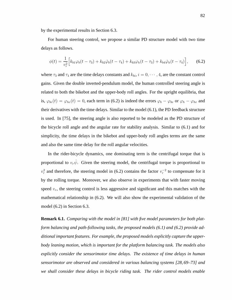
82

by the experimental results in Section 6.3.

For human steering control, we propose a similar PD structure model with two time

delays as follows.

φ(t) =1

v2r

[

kb1ϕb(t− τ3) + kb2ϕb(t− τ4) + kb3ϕh(t− τ3) + kb4ϕh(t− τ4)]

, (6.2)

whereτ3 andτ4 are the time delays constants andkbi, i = 0, · · · , 4, are the constant control

gains. Given the double inverted-pendulum model, the humancontrolled steering angle is

related to both the bikebot and the upper-body roll angles. For the upright equilibria, that

is, ϕbe(t) = ϕhe(t) = 0, each term in (6.2) is indeed the errorsϕb − ϕbe or ϕh − ϕhe and

their derivatives with the time delays. Similar to the model(6.1), the PD feedback structure

is used. In [75], the steering angle is also reported to be modeled as the PD structure of

the bicycle roll angle and the angular rate for stability analysis. Similar to (6.1) and for

simplicity, the time delays in the bikebot and upper-body roll angles terms are the same

and also the same time delay for the roll angular velocities.

In the rider-bicycle dynamics, one dominating term is the centrifugal torque that is

proportional tovrψ. Given the steering model, the centrifugal torque is proportional to

v2r and therefore, the steering model in (6.2) contains the factor v−2

r to compensate for it

by the rolling torque. Moreover, we also observe in experiments that with faster moving

speedvr, the steering control is less aggressive and significant andthis matches with the

mathematical relationship in (6.2). We will also show the experimental validation of the

model (6.2) in Section 6.3.

Remark 6.1. Comparing with the model in [81] with five model parameters for both plat-

form balancing and path-following tasks, the proposed models (6.1) and (6.2) provide ad-

ditional important features. For example, the proposed models explicitly capture the upper-

body leaning motion, which is important for the platform balancing task. The models also

explicitly consider the sensorimotor time delays. The existence of time delays in human

sensorimotor are observed and considered in various balancing systems [28, 69–73] and

we shall consider these delays in bicycle riding task. The rider control models enable

83

the stability analysis of the closed-loop systems. Finally, we also conduct the sensitivity

study of the model parameters under various sensory feedback disturbances. These are

complementary to the results in [81]. Finally, the rider control models are validated by

multiple-subject experiments and the results confirm the human riding performance and

the models.

Remark 6.2. We focus on the platform balancing task in this paper and the rider control

models are proposed by this consideration. Although they are not extensively validated by

path-following experiments, the rider control models in this paper might be possibly mod-

ified for path-following task [78]. Indeed, we have presented a nonlinear control design

(i.e., EIC-based control) for an autonomous bicycle for path-following task [22]. The rider

control outputs (i.e., steering angle) are similar to the EIC-based controller outputs. Ex-

tensive validation of the rider control models for path-following performance is out of the

scope of this study.

Remark 6.3. The steering control model (6.2) takes the steering angle, rather than steer-

ing torque, as its output for several reasons. First, due to the geometry parameters and

mass distributions, the combination of the bicycle rollingmotion and the forward motion

generates the steering torque with self-stability property [77]. However in practical rider

control scenarios, this torque is not large comparing with the steering friction and rider

control torque. The steering dynamics from the rider steering torque input to the steering

angle output has the fast responses. For a conventional bicycle, the steering torque due

to self-stability has negligible influence for the rider control. The rider can easily control

the steering close to the desired motion. Second, the experimental results in Section 6.4 of

this chapter and [21] confirm that the steering angle profilesfit well with the output of the

proposed steering control model. Indeed, besides our work,other reported control design

and experiments such as those in [21, 42] also neglect the steering dynamics and use the

steering angle (rather than the steering torque) as the input to obtain satisfactory results.

Finally, inclusion of the steering dynamics would increasethe complexity of the closed-

loop stability analysis and might even prevent from obtaining the stability and parameter

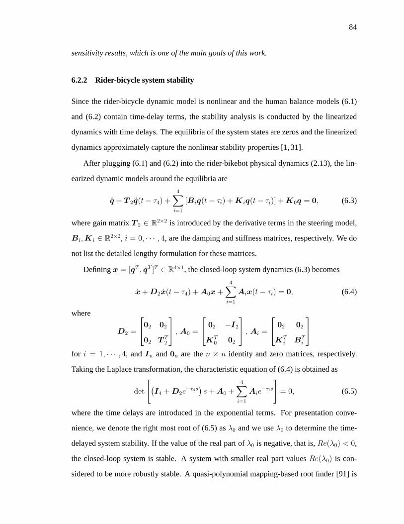
84

sensitivity results, which is one of the main goals of this work.

6.2.2 Rider-bicycle system stability

Since the rider-bicycle dynamic model is nonlinear and the human balance models (6.1)

and (6.2) contain time-delay terms, the stability analysisis conducted by the linearized

dynamics with time delays. The equilibria of the system states are zeros and the linearized

dynamics approximately capture the nonlinear stability properties [1,31].

After plugging (6.1) and (6.2) into the rider-bikebot physical dynamics (2.13), the lin-

earized dynamic models around the equilibria are

q + T 2q(t− τ4) +

4∑

i=1

[Biq(t− τi) + K iq(t− τi)] + K0q = 0, (6.3)

where gain matrixT 2 ∈ R2×2 is introduced by the derivative terms in the steering model,

Bi,K i ∈ R2×2, i = 0, · · · , 4, are the damping and stiffness matrices, respectively. We do

not list the detailed lengthy formulation for these matrices.

Definingx = [qT , qT ]T ∈ R4×1, the closed-loop system dynamics (6.3) becomes

x + D2x(t− τ4) + A0x +

4∑

i=1

Aix(t− τi) = 0, (6.4)

where

D2 =

02 02

02 T T2

, A0 =

02 −I2

KT0 02

, Ai =

02 02

KTi BT

i

for i = 1, · · · , 4, andIn and0n are then × n identity and zero matrices, respectively.

Taking the Laplace transformation, the characteristic equation of (6.4) is obtained as

det

[

(I4 + D2e

−τ4s)s+ A0 +

4∑

i=1

Aie−τis

]

= 0, (6.5)

where the time delays are introduced in the exponential terms. For presentation conve-

nience, we denote the right most root of (6.5) asλ0 and we useλ0 to determine the time-

delayed system stability. If the value of the real part ofλ0 is negative, that is,Re(λ0) < 0,

the closed-loop system is stable. A system with smaller realpart valuesRe(λ0) is con-

sidered to be more robustly stable. A quasi-polynomial mapping-based root finder [91] is

85

used to compute the stability region given by (6.5). We will also useRe(λ0) to illustrate

the stability property in later sections.

6.3 Experiments

In this section, we present the experimental setup, description and performance evaluation.

The experiments in this study serve for several purposes. The experiments are used to test

and validate the rider-bikebot dynamic models and the humanbalance control models dis-

cussed in the previous two sections. Moreover, we conduct experiments to understand and

reveal how the parameters of the human steering and upper-body control models change

under various riding conditions. Finally, we use the experiments to quantify and evaluate

the human riding performance and the stability results.

6.3.1 Riding experiments design

Five subjects were recruited for the experiments. In all tests, the subjects were required

to ride the bikebot only for keeping balance on an open parking field without considering

the bikebot trajectory. Therefore, path-following was notamong the riding objectives. The

bikebot was controlled at a constant speed (ranging from1.7-2.3 m/s and speed variation is

less than0.2 m/s in each test).

The riding experiments were conducted by three groups, following three types of dis-

turbances. The first group was the normal riding with perturbed rolling torques. The rolling

torque disturbance was introduced by the gyro-balancer. The subjects were informed the

possible rolling disturbance but they did not know when the disturbance was applied. The

generated disturbance was an impulse torque by suddenly pivoting of the spinning fly-

wheel. In the second group of experiments, the riders were visually perturbed as well as

the external torque disturbances by the gyro-balancer. To generate the visual disturbances,

two types of eye glasses were wore by the riders separately. Fig. 6.2(b) shows these two

types of eye glasses. The viewed images of the first pair of glasses (called Glasses I) were

86

partially blocked by translucent tapes. The subjects cannot see the environment objects

completely and the sensing images were blocked partially. The images of the second pair

of glasses (called Glasses II) were distorted by a set of internal mirrors. The visual hori-

zontal references were also distorted by Glasses II. When the subjects wore Glasses II, they

felt dizzy with the distorted images and it took a few hours toget used to it but still with

misjudgement sometimes. It is generally considered that Glasses II generate much more

visual and perception distortion and disturbance than thatof Glasses I.

The third set of experiments were conducted with time-delaydisturbances in steering

actuation. In these tests, the handlebar and the front wheelframe were mechanically dis-

connected. The rider rotated the handlebar and the actual steering angle was controlled by

the steering motor to track the human input angle with a designed time delay, as shown in

Fig. 6.2(a). The goal of this set of experiments is to understand how the steering distur-

bance and delay affect the riding performance and stability. The time-delay was set initially

from 80 ms and incremental delay in each experiment was 50 ms until the subjects cannot

maintain balancing properly. These time-delay values are at the same range of the human

neuro-controller delays reported in [28].

We label five subjects as A to E. Each subject was asked to ride the bikebot according to

the above-mentioned three groups of experiments. Before riding data was collected, each

subject was asked to ride the bikebot for about 15 to 30 minutes. Under each experimental

condition, the subject was asked to repeat the tests two or three times and all experimental

data were recorded and processed. All subjects completed the first group of normal riding

experiments and the second group of visual disturbances experiments with wearing Glasses

I. However, subject E cannot ride the bikebot while wearing Glasses II. For the third group

of riding experiments, subject A can ride and keep balance attime delays80, 130, 180, and

230 ms, subjects B and C finished successfully with80, 130, and180 ms, and subjects D

and E can only ride successfully at80 and130 ms.

87

(a) (b)

Figure 6.2: (a) Handlebar and front wheel steering angle sensors and front wheel steeringactuator. (b) Visual blocking glasses and mirror glasses.

6.3.2 Riding Performance Metrics

We use the value ofRe(λ0) of (6.5) as an indicator to quantify the system stability. To

quantify the riding balance skills, we use the BEM concept that was introduced previously

as a performance metric. The basic idea of the BEM is to calculate the balanced bicycle

and rider upper-body roll angles under the human control.

For given rider steering and pedaling inputs, we compute therequired balance torque

by the upper-body motion and these torques due to the bicycleroll motion (due to mass

center position changes). From the first dynamics equation (2.13), if the difference of the

calculated required torque and rider-bicycle rolling torque is zero, the bicycle roll angleϕb

and the rider upper-body roll angleϕh will maintain their equilibria. The calculation of

F (q, φ, φ) captures the net balancing torque for the rider upper-body movement under the

equilibrium conditions,

F (q, uφ) = −mbh2b sϕb cϕb ψ

2 −mhh2h sϕb+ϕh cϕb+ϕh ψ

2 −mhhhhs c2ϕb+ϕh ψ2

+mbhblb cϕb ψ +mhhsls cϕb ψ +mhhhls cϕb+ϕc ψ +mbhb cϕb vrψ

+mhhs cϕb vrψ +mhhh cϕb+ϕh vrψ −mbghb sϕb −mhghs sϕb

−mhghh sϕb+ϕh −uφ,

(6.6)

with uφ = (mblb +mhls)glt cξl

tanφ cϕb .

The smaller value of|F (q, φ, φ)|, the closer of the roll angles to their equilibria. Con-

sidering the metricF (q, φ, φ) over a time interval[t1, t2], we use the following balance

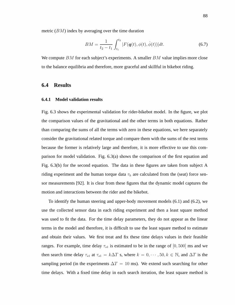
88

metric (BM) index by averaging over the time duration

BM =1

t2 − t1

∫ t2

t1

|F (q(t), φ(t), φ(t))|dt. (6.7)

We computeBM for each subject’s experiments. A smallerBM value implies more close

to the balance equilibria and therefore, more graceful and skillful in bikebot riding.

6.4 Results

6.4.1 Model validation results

Fig. 6.3 shows the experimental validation for rider-bikebot model. In the figure, we plot

the comparison values of the gravitational and the other terms in both equations. Rather

than comparing the sums of all the terms with zero in these equations, we here separately

consider the gravitational related torque and compare themwith the sums of the rest terms

because the former is relatively large and therefore, it is more effective to use this com-

parison for model validation. Fig. 6.3(a) shows the comparison of the first equation and

Fig. 6.3(b) for the second equation. The data in these figuresare taken from subject A

riding experiment and the human torque dataτh are calculated from the (seat) force sen-

sor measurements [92]. It is clear from these figures that thedynamic model captures the

motion and interactions between the rider and the bikebot.

To identify the human steering and upper-body movement models (6.1) and (6.2), we

use the collected sensor data in each riding experiment and then a least square method

was used to fit the data. For the time delay parameters, they donot appear as the linear

terms in the model and therefore, it is difficult to use the least square method to estimate

and obtain their values. We first treat and fix these time delays values in their feasible

ranges. For example, time delayτs1 is estimated to be in the range of[0, 500] ms and we

then search time delayτs1 at τs1 = k∆T s, wherek = 0, · · · , 50, k ∈ N, and∆T is the

sampling period (in the experiments∆T = 10 ms). We extend such searching for other

time delays. With a fixed time delay in each search iteration,the least square method is

89

28 30 32 34 36 38

-100

-50

0

50

100Non-gravityGravity

Time (s)

Torq

ue(N

m)

(a)

28 30 32 34 36 38-30

-20

-10

0

10

20

30Non-gravity

Gravity

Time (s)

Torq

ue(N

m)

(b)

Figure 6.3: Experimental results for rider-bikebot dynamics models validation. (a) Balanc-ing torques in the first equation of rider-bikebot dynamics.(b) Balancing torques in thesecond equation of rider-bikebot dynamics.

then used for estimating and obtaining the values of the control gains. For each set of

estimated time delays and control gains, we compute the fitting errors. Finally, the set of

the parameters that gives the smallest fitting error is chosen as the estimates of the control

model parameters.

Fig. 6.4 shows the validation results in one experiment testby subject A. The model

parameters were obtained by using the data collected in other experimental runs. The rider

operated the bikebot in a straight line like trajectory and the bikebot roll angle was within

0.1 rad; see Fig. 6.4(a). The model predictions of the steering angleφ and upper-body

movement torqueτh follow the sensor measurements in experiments. These results con-

firm the human steering and upper-body movement models. Similar to the dynamic model

validation, we also calculated the aggregated relative errors between the model prediction

and experiments shown in Fig. 6.4. For most of the riding experiments, the relative errors

for the steering angle and upper-body leaning torque are less than 35% and 10%, respec-

tively, for a 10 s time duration as shown in the figure.

We estimate the model parameters in (6.1) and (6.2) for each subject. The parameter

values are listed in Table 6.1 for the gains and Table 6.2 for the time delays. In the tables, we

include the mean values and standard deviations of each model parameter and time delay.

From the magnitudes of these parameters in the tables, we obtain that for the upper-body

90

movement torque (6.1), the values of passive stiffness parameterkh0 are slightly smaller

than these of active controlledkh3. Both kh0 andkh3 are larger than the control gainkh1.

Model parameterkh2 is also smaller thankh4. Therefore, the rider leaning torque is much

more sensitive for the upper-body attitude than the bikebotattitude. The time delay of the

steering control has an overall much larger value than that of the upper-body movement,

similar to the previously reported results [93] in which theformer and latter delays are

around 200 and 100 ms, respectively.

28 30 32 34 36 38

-0.1

0

0.1

0.2

-22 -20 -18 -16 -14 -12 -10 -8 -6 -41

2

3

4

5

6Time (s)

X (m)

Y(m

)ϕb/ϕh

(rad

) ϕbϕh

(a)

-0.5

0

0.5

ExpModel

28 30 32 34 36 38

-20

0

20

Time (s)

τ h(N

m)

φ(r

ad)

(b)

Figure 6.4: Rider steering and upper-body movement model validation results. (a) Riderupper-body and bikebot roll angle profiles (top plot) and bikebot position trajectory (bottomplot). (b) Validation results for the rider steering control modelφ in (6.2) (top plot) and theupper-body movement torque modelτh in (6.1) (bottom plot).

Table 6.1: The mean and standard deviation of the human steering and upper-body move-ment model parameters.

Gains A B C D Ekh0 −96.3 ± 6.03 −97.7 ± 7.50 −99.5 ± 12.0 −81.0 ± 3.82 −80.0 ± 3.54kh1 −66.2 ± 8.37 −71.5 ± 8.03 −74.6 ± 9.88 −84.0 ± 8.78 −81.9 ± 5.51kh2 −8.23 ± 0.85 −7.13 ± 6.03 −10.3 ± 1.56 −4.2 ± 1.84 −9.0 ± 0.95kh3 −139 ± 6.55 −135 ± 3.51 −111 ± 22.6 −85.0 ± 5.66 −75.7 ± 4.96kh4 −19.6 ± 0.75 −13.0 ± 2.27 17.7 ± 5.87 −11.7 ± 2.40 −16.9 ± 1.31kb1 10.15 ± 0.54 10.53 ± 0.51 9.13 ± 0.28 10.06 ± 0.15 10.10 ± 0.64kb2 1.24 ± 0.85 1.13 ± 0.06 1.62 ± 0.269 1.07 ± 0.028 1.61 ± 0.48kb3 0.90 ± 0.20 0.83 ± 0.06 1.33 ± 0.42 0.79 ± 0.23 1.30 ± 0.28kb4 0.92 ± 0.36 1.18 ± 0.13 1.01 ± 0.25 1.00 ± 0.28 1.18 ± 0.32

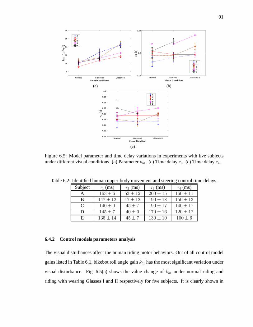
91

Normal Glasses I Glasses IIVisual Conditions

8

10

12

14

16

18

ACBDE

kb1

(m2/s

2)

(a)

Normal Glasses I Glasses IIVisual Condition

0.15

0.2

0.25

ACBDE

τ 3(s

)

(b)

Normal Glasses I Glasses IIVisual Condition

0.12

0.13

0.14

0.15

0.16

0.17

0.18

0.19

0.2

ACBDE

τ 4(s

)

(c)

Figure 6.5: Model parameter and time delay variations in experiments with five subjectsunder different visual conditions. (a) Parameterkb1. (c) Time delayτ3. (c) Time delayτ4.

Table 6.2: Identified human upper-body movement and steering control time delays.Subject τ1 (ms) τ2 (ms) τ3 (ms) τ4 (ms)

A 163 ± 6 53 ± 12 200 ± 15 160 ± 11B 147 ± 12 47 ± 12 190 ± 18 150 ± 13C 140 ± 0 45 ± 7 190 ± 17 140 ± 17D 145 ± 7 40 ± 0 170 ± 16 120 ± 12E 135 ± 14 45 ± 7 130 ± 10 100 ± 6

6.4.2 Control models parameters analysis

The visual disturbances affect the human riding motor behaviors. Out of all control model

gains listed in Table 6.1, bikebot roll angle gainkb1 has the most significant variation under

visual disturbance. Fig. 6.5(a) shows the value change ofkb1 under normal riding and

riding with wearing Glasses I and II respectively for five subjects. It is clearly shown in

92

0.00 0.08 0.13 0.18 0.237

7.5

8

8.5

9

9.5

10

10.5

11

11.5

12

A

C

B

D

E

τs (s)

kb1

(m2/s

2)

(a)

0.00 0.08 0.13 0.18 0.230.1

0.12

0.14

0.16

0.18

0.2

0.22

0.24

ACBDE

τs (s)

τ 3(s

)

(b)

0.00 0.08 0.13 0.18 0.230.08

0.1

0.12

0.14

0.16

0.18

0.2

ACBDE

τs (s)

τ 4(s

)

(c)

0.00 0.08 0.13 0.18 0.23-110

-100

-90

-80

-70

-60

-50

-40

ACBDE

τs (s)

kh1

(Nm

/rad

)

(d)

0.00 0.08 0.13 0.18 0.230.15

0.2

0.25

0.3

0.35

0.4

A

C

B

D

E

τs (s)

τ s3

(s)

(e)

0.00 0.08 0.13 0.18 0.230.1

0.15

0.2

0.25

0.3

0.35

ACBDE

τs (s)

τ s4

(s)

(f)

Figure 6.6: Control model parameters and human steering time delays under varying steer-ing actuation delayτs. (a) Human steering control gainkb1. (b) Total steering delayτs3.(c) Total steering delayτs4. (d) Human upper-body control gainkb1. (e) Human steeringcontrol delayτ3. (f) Human steering control delayτ4.

these plots that after blocking the visual feedback, the values of gainkb1 increase about 0.5-

2 consistently for each subject. Moreover, when the subjects wear Glasses II that distort

the visual feedback information, the values ofkb1 increase further about additional 0.5-2

for four out of five subjects. (The fifth subject E cannot ride stably.) Figs. 6.5(b) and 6.5(c)

further show the values of time delaysτ3 andτ4 under visual disturbances.

93

We ran theF -test (with null hypothesis rejection probability0.05) of kb1 variation under

visual disturbances to determine whether the visual conditions changing is the main cause

for the parameters variations. The results confirm that the visual conditions significantly

influence subjects A, B and C, while the effect was not clearlyobserved for subject D

(subject E failed to ride when wearing Glasses II). We do not find statistically significant

changes of other control gains or time delays under visual disturbances.

For the last group of experiments with delayed steering actuation, we denote the steer-

ing actuation time delay asτs. With human control delaysτ3 and τ4 in (6.2), the total

steering time delays are defined as

τs3 = τ3 + τs, τs4 = τ4 + τs.

Under varyingτs (i.e., τs3 and τs4), we have observed the changing values of steering

control gainkb1 and leaning control gainkh1, and time delaysτ3 andτ4. These observations

are illustrated in Fig. 6.6. We particularly illustrate these parameters because their changes

are the most significant.

Fig. 6.6(a) shows a seemingly decreasing trend of the human steering control gainkb1

with increasingτs. This could imply that the riders enforce the dominating steering gain

slightly by noticing the total time delays. However, this decreasing trend is not statistically

significant. We have obtained that only subject B shows the significant decrease and all

other subjects do not. The absolute values of the human control gain kh1 in Fig. 6.6(c)

instead show an increasing trend withτs. Comparing with the values in normal riding

case, the values of|kh1| at τs = 230 ms increase about 20 percent. It seems that with

an increasedτs, the riders tried to use their upper-body movement aggressively to keep

balancing the platform.

It is interesting to observe the decreasing trends of time delays τ3 and τ4 shown in

Figs. 6.6(b) and 6.6(c), respectively. We verified this tendency hypothesis by conducting

anF -test. For example, forτ3, theF -test results for subjects A and B are positive. But

the results for subjects C, D and E are negative. This result is likely due to the fact that

94

subjects D and E cannot even ride the bikebot onceτs > 130 ms. Similarly, forτ4, the

F -test results show that subjects A, B, and C are significant but not D and E. A large value

of τs implies an increased difficulty of riding bikebot. Only subject A can ride on the

bikebot atτs = 230 ms. Subjects B and C can still ride the bikebot up toτs = 180 ms and

D and E atτs = 130 ms. Although all subjects have different handling capabilities, it is

interesting to note in Figs. 6.6(e) and 6.6(f) that the maximum total time delaysτs3 andτs4

of all subjects are about the same, that is, around350 ms and400 ms, respectively. These

limits are probably the hard capability of the longest steering delay for experienced human

riders. It is also interesting to note that during theτs-increasing process, the values of delay

τ3 are consistently larger than those ofτ4 around 20 ms.

To analyze the trend across all subjects, Fig. 6.7 shows the mean values and standard

deviations of the above-mentioned parameters under varying τs and visual conditions. We

used the analysis of variance method to compute the mean and variance values for each

variable in the figure. We clearly see a decreasing trend for gainskb1, kh1, and time delays

τ3 andτ4 with increasingτs as shown in the top three plots in Fig. 6.7. Under increasing

severity of the visual conditions, the values of gainkb1 also increase as shown in the bottom

plot in Fig. 6.7. We conduct anF -test for the above-mentioned tendency hypotheses and

statistically only gainkb1 and delayτ4 show significantly changes under visual disturbance

and increasingτs, respectively.

We calculate the balance metricBM under different riding conditions and Fig. 6.8

shows the mean and standard deviation values. Fig. 6.8(a) showsBM calculations for

all subjects with increasingτs. The values ofBM clearly increase withτs. TheBM

values are around20 Nm for most riders (except subject E) at normal riding condition, i.e.,

τs = 0. Whenτs = 230 ms, theBM values increase to around30-60 Nm. Similarly, the

BM values also reach to around35-50 Nm when the subject wears Glasses II as shown

in Fig. 6.8(b). The deteriorated balance performance, thatis, increasedBM values, under

varying riding conditions (either large delay or severe visual distortion) match the riding

difficulty reported by the subjects.

95

8

10

12

-100

-50

0.00 0.08 0.13 0.18 0.23

0.1

0.2

0.3

Normal Glasses I Glasses II

Visual Condition

10

15

kb1

(m2/s

2)

kh1

(Nm

/rad

)τ

(s) τ3

τ4

kb1

(m2/s

2)

τs (s)

Figure 6.7: Mean values and standard deviations across all subjects with respect to experi-ments conditions.

0.00 0.08 0.13 0.18 0.230

10

20

30

40

50

60

70

ACBDE

τs (s)

BM

(Nm

)

(a)

Normal Glasses I Glasses IIVisual Condition

5

10

15

20

25

30

35

40

45

50

55

A

C

B

D

E

BM

(Nm

)

(b)

Figure 6.8: Balance metricBM (mean and standard deviation) for five subjects under (a)varying steering actuation delayts and (b) visual conditions.

6.4.3 Stability results

From experiment observations, time delaysτs3 andτs4 are critical to system stability. We

here choose gainskb1 andkb2 of the human steering control model (6.2) as an example to

illustrate the stability analysis. Fig. 6.9 shows the stability region in thekb1-kb2 plane under

delayτs3 = 200, 300 and350 ms. The stability region is defined asRe(λ0) < 0 for the

roots of (6.5) under changing model parameters, in this case, kb1 andkb2. The values of

all other model parameters and delays are listed in Tables 6.1 and 6.2. From Note that by

Fig. 6.6(e), the range ofτs3 ∈ [200, 350] ms corresponds to steering delayτs ∈ [0, 230]

96

ms. Besides the plotted regions (as solid red lines) by usingthe mean values of all model

parameters and delays, we also include the stability regions using the sets of the model

parameters one standard deviation smaller (green dot lines) and larger (blue dash lines)

than the mean values.

Fig. 6.9(a) shows the stability region whenτs3 = 200 ms, that is, zero delayτs =

0, while Figs. 6.9(b) and 6.9(c) forτs3 = 300 ms andτs3 = 350 ms, respectively. By

comparing these figures, we clearly observe that: (1) with increasingτs, the size of the

stability region reduces as shown fromτs = 0 (i.e.,τs3 = 200 ms) in Fig. 6.9(a) toτs = 230

ms (i.e.,τs3 = 350 ms) in Fig. 6.9(c). This is reasonable since it is more difficult for a

rider to balance a bikebot with a long steering delay than that with a short delay; (2) It is

interesting to see the identified(kb1, kb2) locations for each individual subject are relative

to the boundaries of the stability regions in the figure: withincreasing delays, the subjects’

balance performance became deteriorated and in the case ofτs = 230 ms in Fig. 6.9(c),

all subjects performed closely around the stability regionboundary. This is not surprised

since as shown in Fig. 6.6(e),τs3 = 350 ms (τ3 = 230 ms) is the maximum total (actuation)

delay that all subjects can handle without loss of balance inthe riding experiments.

Similar to Fig. 6.9 to show the stable regions under different values of the control gains,

Fig. 6.10 illustrates the stable region in theτs3 − τs4 plane along with all the subject time

delays. The plots are split into three groups according to the introduced threeτs3 ranges

between 160 and 400 ms. The figures give an estimation of the ranges of the time delays

τs3 andτs4 for system stability and also the observed subjects time delays. We also see that

for almost all experiments, the subject time delays are located within but close to the stable

region boundaries.

The values ofRe(λ0) with varying τs3 andτs4 are shown in Fig. 6.11(a). From this

figure, the values ofRe(λ0) are much more sensitive withτs3 (τ3) rather thanτs4 (τ4).

VariableRe(λ0) has the minimum value at aroundτs3 = 330 ms. The stability region is

plotted in Fig. 6.11(d) and from the figure, the maximal valueof τs3 for a stable closed-

loop system is about375-380 ms. This result is consistent with the experiment observation

97

shown in Fig. 6.6(d). In the experiments, no subject can control and balance the bikebot

whenτs3 > 400 ms and the maximum total delayτs3 for all subjects is about350 ms.

To clearly see the dependency of control gainkb1 on delayτs3, Fig. 6.11(b) shows the

Re(λ0) values as varyingkb1 andτs3 and Fig. 6.11(e) illustrates the stability region in the

kb1-τs3 plane. The stability region clearly confirms that the value of kb1 is reduced when

delay τs3 increases. Figs. 6.11(c) and 6.11(f) show theRe(λ0) and the stability regions

under varyingτ1 andτ2 with zero delayτs. For the pair(τ1, τ2) by which the system is stable

as shown in Fig. 6.11(f), the values ofRe(λ0) have no significant change. This implies that

system stability is not sensitive for(τ1, τ2) in these ranges. The values ofRe(λ0) and the

stability regions of varying gainskh1 andkh2 are demonstrated in Figs. 6.12(a)-6.12(b)

respectively forτs3 = 200 and350 ms. The stability regions are highly influenced byτs3

andτs4. With large time delays, the control gainkh1 is bounded and the absolute values of

kh1 from the experiments in Fig. 6.6(d) show an increasing and bounded trend as well.

6.5 Discussions

The human upper-body movement model (6.1) includes only thedependency on bikebot

and upper-body roll angles and their derivatives. Some other influencing factors are ne-

glected in this model. For instance, different from the quiet stance, the moving bikebot

is a non-inertial frame and thus, the Coriolis and centrifugal accelerations have influences

on the applied balance torques. At low moving velocities, yaw angleψ does not change

dramatically and the termψ2 can be neglected. We also neglect the possible influence of

the steering action on the upper-body movement torqueτh in the model.

We compare the human model parameters in bikebot riding withthe stationary riding

experiments in [31] and the stance experiments in [28]. First, the observed time delays

are not the same values as these in [28, 31]. In [28, 31], threetime delays, i.e., short-,

medium- and long-latency processes, are introduced in the model with the mean values

around21, 131 and288 ms, respectively. The short- and medium-latency processesare

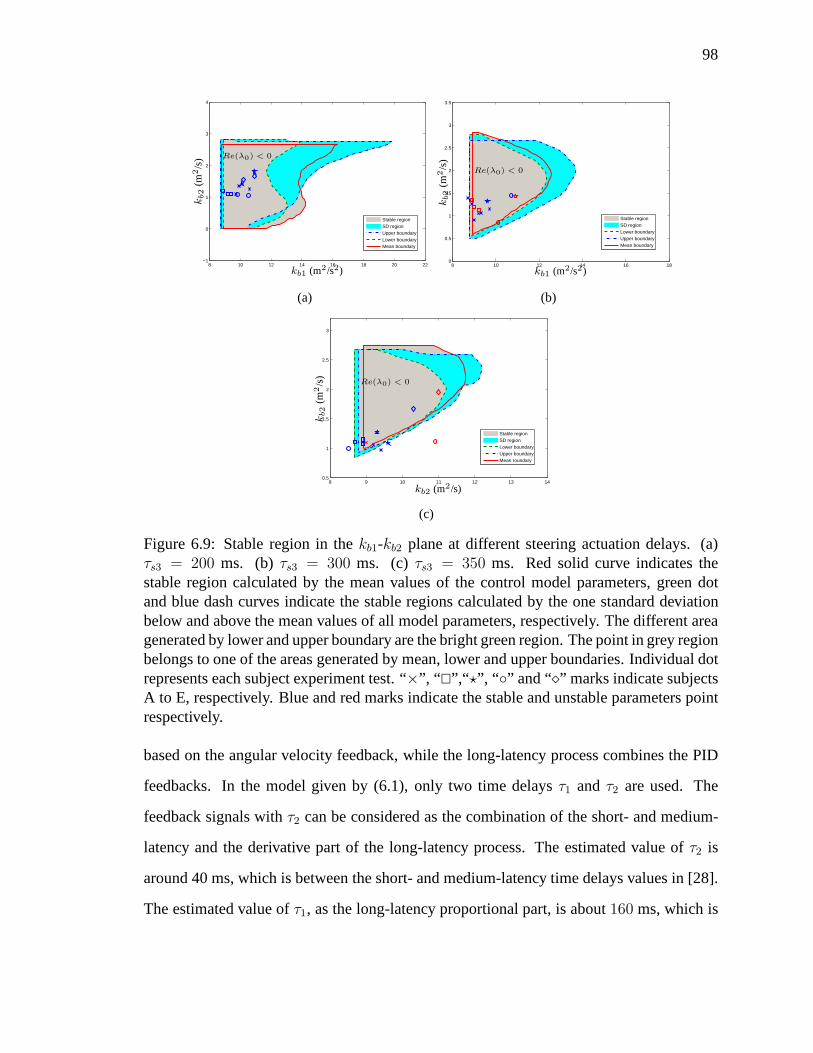
98

8 10 12 14 16 18 20 22−1

0

1

2

3

4

Stable regionSD regionUpper boundaryLower boundaryMean boundary

kb1 (m2/s2)

kb2

(m2/s

) Re(λ0) < 0

(a)

8 10 12 14 16 180

0.5

1

1.5

2

2.5

3

3.5

Stable regionSD regionLower boundaryUpper boundaryMean boundary

kb1 (m2/s2)

kb2

(m2/s

)

Re(λ0) < 0

(b)

8 9 10 11 12 13 140.5

1

1.5

2

2.5

3

Stable regionSD regionLower boundaryUpper boundaryMean roundary

kb2

(m2/s

)

kb2 (m2/s)

Re(λ0) < 0

(c)

Figure 6.9: Stable region in thekb1-kb2 plane at different steering actuation delays. (a)τs3 = 200 ms. (b) τs3 = 300 ms. (c) τs3 = 350 ms. Red solid curve indicates thestable region calculated by the mean values of the control model parameters, green dotand blue dash curves indicate the stable regions calculatedby the one standard deviationbelow and above the mean values of all model parameters, respectively. The different areagenerated by lower and upper boundary are the bright green region. The point in grey regionbelongs to one of the areas generated by mean, lower and upperboundaries. Individual dotrepresents each subject experiment test. “×”, “ @”,“ ⋆”, “ ” and “⋄” marks indicate subjectsA to E, respectively. Blue and red marks indicate the stable and unstable parameters pointrespectively.

based on the angular velocity feedback, while the long-latency process combines the PID

feedbacks. In the model given by (6.1), only two time delaysτ1 and τ2 are used. The

feedback signals withτ2 can be considered as the combination of the short- and medium-

latency and the derivative part of the long-latency process. The estimated value ofτ2 is

around 40 ms, which is between the short- and medium-latencytime delays values in [28].

The estimated value ofτ1, as the long-latency proportional part, is about160 ms, which is

99

0 0.1 0.2 0.3 0.4 0.5 0.6 0.7 0.8 0.9 10

0.05

0.1

0.15

0.2

0.25

0.3

Re(λ0) < 0

τs4 (s)

τ s3

(s)

(a)

0 0.1 0.2 0.3 0.4 0.5 0.6 0.7 0.8 0.9 10

0.1

0.2

0.3

0.4

Re(λ0) < 0

τs4 (s)

τ s3

(s)

(b)

0 0.1 0.2 0.3 0.4 0.5 0.6 0.7 0.8 0.9 10

0.1

0.2

0.3

0.4

Re(λ0) < 0

τs4 (s)

τ s3

(s)

(c)

Figure 6.10: Stable region in theτs4-τs3 plane at different steering actuation delays. (a)τs3 ∈ [160, 240) ms. (b)τs3 ∈ [240, 320) ms. (c)τs3 ∈ [320, 400] ms. Grey area indicatesthe stable region calculated by the mean values of the control model parameters. (Allexperiments trails are divided into 3 sets corresponding theseτs3 intervals. In every group,the average value of the upper-body time delays and all the control gains generate the greyareas.) In the figures, individual dot represents each subject experiment test. “×”, “ @”,“ ⋆”,“” and “⋄” marks indicate subjects A to E, respectively. Blue and red marks indicate thestable and unstable parameters point respectively.

smaller than that of long-latency time288 ms in [28]. The estimated value of the upper-

body passive stiffnesskh0 (see Table 6.1) in the bikebot riding experiments is larger than

that ofKin = 73.5 Nm/rad in [28], where the proportional control gainkh3 is close to the

value ofKin = 149 Nm/rad in [28]. The value of the upper-body angular velocitycontrol

gainkh4 is smaller than that ofBsl +Bv = 45.6 Nm/rad in the stance model.

From Table 6.1, the value of gainkb1 for bikebot roll angleϕb is much larger than that

of gain kb3 for the upper-body roll angleϕh. The angular velocity gainskb2 andkb4 are

within a similar range. Considering the magnitudes ofϕb, ϕh and their derivatives, the

dominating term of (6.2) is the first one, that is,kb1ϕb. This implies that the roll angle

ϕb plays a more important role for balancing the platform thanϕh does. From Table 6.2,

the values of time delaysτ3 (angular feedback) andτ4 (angular velocity feedback) in the

human steering control are about (around50 and100 ms) larger respectively than those

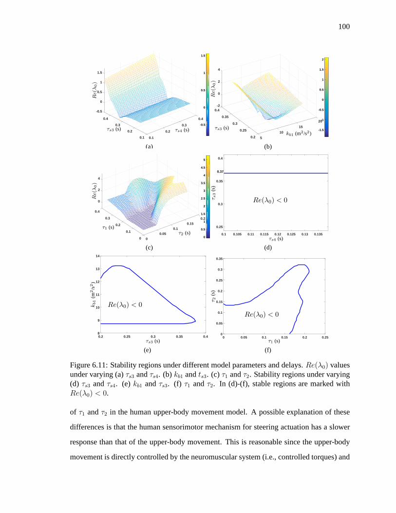
100

-0.5

0

0.4 0.4

0.5

0.3 0.3

1

1.5

0.2 0.2

0.1 0.1

-0.5

0

0.5

1

1.5

τs3 (s) τs4 (s)

Re(λ0)

(a)

-20.4

0.35

0

200.3

2

150.25 10

4

0.2 5

-1.5

-1

-0.5

0

0.5

1

1.5

2

kb1 (m2/s2)τs3 (s)

Re(λ0)

(b)

0.4

0

0.3 0.20.150.2

2

0.10.1

0.05

4

0 0 0

0.5

1

1.5

2

2.5

3

3.5

4

4.5

5

τ1 (s)τ2 (s)

Re(λ0)

(c)

0.1 0.105 0.11 0.115 0.12 0.125 0.13 0.135

0.25

0.3

0.35

0.4

0.37

τ s3

(s)

τs4 (s)

Re(λ0) < 0

(d)

0.2 0.25 0.3 0.35 0.48

9

10

11

12

13

14

kb1

(m2/s

2)

τs3 (s)

Re(λ0) < 0

(e)

0 0.05 0.1 0.15 0.2 0.250

0.05

0.1

0.15

0.2

0.25

0.3

0.35

τ1 (s)

τ 2(s

)

Re(λ0) < 0

(f)

Figure 6.11: Stability regions under different model parameters and delays.Re(λ0) valuesunder varying (a)τs3 andτs4. (b) kb1 andts3. (c) τ1 andτ2. Stability regions under varying(d) τs3 andτs4. (e) kb1 andτs3. (f) τ1 andτ2. In (d)-(f), stable regions are marked withRe(λ0) < 0.

of τ1 andτ2 in the human upper-body movement model. A possible explanation of these

differences is that the human sensorimotor mechanism for steering actuation has a slower

response than that of the upper-body movement. This is reasonable since the upper-body

movement is directly controlled by the neuromuscular system (i.e., controlled torques) and

101

the steering actuation is through the limb movements (i.e.,controlled angles) with possible

longer time delays.

-10

0

1

-50

2

0

3

-20-100

4

-40-150 -60

0

0.5

1

1.5

2

2.5

3

kh1 (Nm/rad)

kh2 (Nms/rad)

Re(λ0)

(a)

-150

0

-60-100

1

-40-50

2

-20

0 0

-0.5

0

0.5

1

1.5

2

kh1 (Nm/rad)kh2 (Nms/rad)

Re(λ0)

(b)

Figure 6.12:Re(λ0) values under varyingkh1 andkh2 with (a)τs3 = 200 ms andτs4 = 160ms and (b)τs3 = 350 ms andτs4 = 310 ms.

To observe the influence of steering delays onτ1 andτ2, Fig. 6.13 illustrates the stability

regions in theτ1-τ2 plane under four different pairs of(τs3, τs4): (200, 160), (250, 210),

(300, 260), and (350, 310) ms, respectively. We choose these pairs of(τs3, τs4) values

because the adjacent pairs are 50-ms incremental each otherand the starting pair is around

τs = 0. From the figure, the stability region is enlarged for the large values of(τs3, τs4).

The maximum value ofτ1 has increased almost around50 ms for each incremental pair of

(τs3, τs4) but the maximum values ofτ2 do not change significantly under varying(τs3, τs4).

The identified values forτ1 andτ2 listed in Table 6.2 all fall into the stability regions and

indeed these values do not change much when the steering delay τs was introduced in

experiments. This could imply that the human riders prefer to use and adopt faster steering

actions, rather than upper-body movement, to respond the time delays produced by the

actuator. This observation is consistent with the sensitivity analysis reported in [22].

Comparing with other sensing modality, the visual feedbackis important for bikebot

balance control. The visual sensing is critical for the rider to obtain the bikebot roll angle

ϕb estimation. Proprioception sensing is used by the rider to detect the body joints angles

and then to estimate the upper-body roll angleϕh. The vestibular feedback allows subjects

to obtain the absolute roll movements. It is possible that other human sensing capabilities

102

0 0.05 0.1 0.15 0.2 0.25 0.3 0.350

0.05

0.1

0.15

0.2

0.25

0.3

0.35

BBBBBBBBBBBBBB CCCCCCCCCCCCCC DDDDDDDDDDDDDD

τs3/τs4 = 200/160ms

Re(λ0) < 0

τ1 (s)

τ 2(s

)

Figure 6.13: Stability regions under under varyingτ1 andτ2 with different delaysτs3 andτs4. The stable region is marked withRe(λ0) < 0. Blue “@”, green “×”, red “⋄”, and black“” marks indicate the estimated mean values of(τ1, τ2) for each subject under these fourpairs of time delay combinationsτs3/τs4, respectively.

(e.g., force) can also provide indirect attitude or pose estimation [92]. However, these per-

ceptions sensory feedbacks cannot be used to completely replace the visual feedback. As

shown in Fig. 6.5, one subject cannot ride the bikebot after wearing Glasses II. This ob-

servation confirms that visual feedback plays a critical role in bikebot riding. On the other

hand, all five subjects can balance the bikebot even with partially visual blocking or distor-

tion and four of them can ride with wearing Glasses II. This implies that other perceptions

capabilities aforementioned can partially substitute thevisual feedback to achieve balance

motor skills. Meanwhile, as an evidence, the value of upper-body movement control gain

kb1 increases when the visual feedback information is partially lost (by Glasses I) and then

further grows when wearing Glasses II. The trend of the increased upper-body movement

control gain complements the visual feedback loss. This is similar to the experiments ob-

servation reported in [28].

The work in this study has several limitations. First, we only recruited experienced

bicycle riders as the subjects and it is not clear whether thepresented results can be ex-

tended and applied to other types of bicycle riders. Second,the results do not include

detailed stability analysis of the influence of bikebot velocity vr. Finally, this paper does

103

not consider and discuss how to tune and adapt the human motorskills through the physi-

cal rider-bikebot interactions. Indeed, all these limitations are among the ongoing research

directions and we will report the new developments in futurepublications.

6.6 Balancing stability under zero speed

For the stationary balancing, the upper-body leaning torque control modelτh is same

as (6.1) in the moving case. Modified from (6.2), the steeringmodel is considered as

φ(t) = kb1ϕb(t− τ3) + kb2ϕb(t− τ4) + kb3ϕh(t− τ3) + kb4ϕh(t− τ4). (6.8)

Plugging (6.1) and (6.8) into the rider-bicycle balance dynamics, we have the linearized

closed-loop dynamic models around the equilibria as

q +4∑

i=1

[B∗i q (t− τi) + K∗

iq (t− τi)] + K∗0q = 0. (6.9)

B∗i ,K

∗i ,K

∗0 ∈ R2×2, i = 1, · · · , 4, are the damping and stiffness matrices, respectively.

Introducingx = [qT , qT ]T , (6.9) becomes

x + A∗0x +

4∑

i=1

A∗ix(t− τi) = 0, (6.10)

where

A∗0 =

02 −I2

(K∗0)T

02

,A∗i =

02 02

(K∗i )T (B∗

i )T

for i = 1, · · · , 4. Taking the Laplace transformation, the characteristic equation of (6.10)

is obtained as

det

(

I4s+ A∗0 +

4∑

i=1

A∗i e

−τis

)

= 0. (6.11)

The QPMR tool is also used to compute the stability region. The control gains and time

delays of the control models (6.8) and (6.1) are estimated and listed in the following:kh0 =

−228.6 N/rad,kh1 = −2482.1 N/rad,kh2 = −305.5 Ns/rad,kh3 = −2253.5 N/rad,kh4 =

−108.7 Ns/rad,kb1 = −523.0, kb2 = −81.5 s,kb3 = −202.6, kb4 = −24.4 s,τ1 = 60 ms,

τ2 = 10 ms,τ3 = 180 ms, andτ4 = 90 ms.

104

We here briefly analyze the system stability around these parameter values. First, under

zero time delaysτi = 0, i = 1, · · · , 4, the closed-loop system is controllable under (6.8)

and (6.1) with these gains values listed above. By using the QPMR method, the stable

regions for time delays parameters are calculated. We also computeRe(λ0) under varying

model parameters. Moreover, under the given control gains and time delays, the closed-

loop system is stable at the upright position. Comparing with the moving bicycle experi-

ments, the control gain values are much larger and the time delays are smaller. This could

be explained by several factors. Without yaw motion, the balancing torque generated by

steering motion is given only byuφ. For a given steering angle, the value ofuφ is much

smaller than the balancing torque generated by yaw motion ofthe under moving platform.

For the stationary case, the upper-body movement contributes more for balancing the plat-

form than the steering actuation. Therefore, the control gain values of the steering and

upper-body movement torque models have large values in stationary case. Moreover, the

system is much more sensitive for the time delays in stationary case than the moving plat-

form because the balance response needs to be faster than that under the moving platform.

Fig. 6.14 illustrates the control parameters sensitivity for stability and stable regions.

Figs. 6.14(a) and 6.14(b) show the changes ofRe(λ0) values with time delay pairs(τ3, τ4)

and(τ1, τ2), respectively, while Figs. 6.14(e) and 6.14(f) illustratethe stable regions over

time delays in models (6.8) and (6.1), respectively. Clearly, these figures show thatRe(λ0)

values change dramatically near the stable boundaries shown in Figs. 6.14(e) and 6.14(f).

This implies that the system stability is sensitive with thetime delays near the boundaries.

Comparing with the regions in the moving bicycle case, the stable regions are smaller in

size. For example, the maximum value ofτ1 is less than 10 ms. For the steering control,

under a givenτ3 the stable interval ofτ4 values is small. Figs. 6.14(c) and 6.14(d) show

theRe(λ0) values under pairs(kb1, kb2) and(kh1, kh2), respectively, and their stable regions

are demonstrated in Figs. 6.14(g) and 6.14(h) accordingly.Near the boundaries, theRe(λ0)

value does not change significantly rapid with these controlgains as those for time delays

in Figs. 6.14(a) and 6.14(b).

105

00.05

0.10.15

0.2

00.1

0.20.3

0.4−5

0

5

−2

−1

0

1

2

3

4

5

τ3 (s)τ4 (s)

Re(λ

0)

(a)

00.02

0.04

00.05

0.10.15

0.2

−5

0

5

10

15

20

0

5

10

15

τ1 (s)τ2 (s)

Re(λ

0)

(b)

5070

90110

300

500

700

−4

0

4

−2

−1

0

1

2

3

4

5

6

kb1 (m2/s2)kb2 (m2/s)

Re(λ

0)

(c)

−360−320

−280−240

−3,500−3,000

−2,500−2,000

−1,500−4

−2

0

2

4

−3

−2

−1

0

1

2

3

kh1 (Nm)kh2 (Nms)

Re(λ

0)

(d)

0 0.05 0.1 0.15 0.2 0.250

0.02

0.04

0.06

0.08

0.1

0.12

0.14

0.16

τ 4(s

)

τ3 (s)

Re(λ0) < 0

(e)

0 0.004 0.008 0.0120

0.02

0.04

0.06

0.08

0.1

τ 1(s

)

τ2 (s)

Re(λ0) < 0

(f)

−95 −90 −85 −80 −75 −70 −65 −60

−760

−720

−680

−640

−600

kb1

(m2/s

2)

kb2 (m2/s)

Re(λ0) < 0

(g)

−400 −350 −300 −250−2,800

−2,600

−2,400

−2,200

−2,000

−1,800

kh1

(Nm

)

kh2 (Nms)

Re(λ0) < 0

(h)

Figure 6.14: Stability regions under different model parameters in zero speed case.Re(λ0)values under varying (a)τ3 andτ4. (b) τ1 andτ2. (c) kb1 andkb2. (d) kh1 andkh2. In (e)-(h),stable regions are marked withRe(λ0) < 0.

106

6.7 Conclusion

This chapter presented the human balance control and stability analysis of the rider-bicycle

systems. We first presented a rider-bikebot dynamic model. Inspired by the experimental

observation and the postural stance balance model, we proposed new PD feedback feedback

models with time delays for the human upper-body movement and steering control for

bicycle riding. The riding experiments with visual feedback and actuation disturbances

were then conducted. We discussed the stability analysis ofthe rider-bicycle system and

presented the influence of the model parameters, including the physical parameters, control

gains and time delays, on the system stability. The results were also used to interpret the

human balance capability and to compare with stance balanceand balancing stationary

bicycles that were reported previously. Additionally, therider-bikebot system balancing

stability in stationary case was also discussed.

107

Chapter 7

Balance Performance Tuning of Rider-BikebotInteractions

7.1 Introduction

Human balance control plays a central role not only in human motor skills, such as stand-

ing or walking, but also in other human-machine or human-robot interactions. In recent

years, bicycle was used as a diagnosis and treatment tool forclinic applications [63]. This

motivates us to use the bicycle-based platform as a tool to study human-machine interac-

tions. Human motor skill tuning or adaptation is another motivation for studying physical

rider-bikebot interactions [66].

Rider motor skills analysis and bicycle self-balance control are two important tasks for

designing balance tuning of rider-bikebot interactions. Bicycle dynamic models are exten-

sively studied (e.g., [16]), and the rider-bicycle dynamicmodels and balance analysis are

also reported in [12, 29, 30]. Several researchers focus on the quantitative modeling and

analysis of riding motor skills. In [21], the rider balance control is modeled as the time

delayed PD feedback for steering and upper-body leaning motion. The work in Chapter 6

extends these control models with sensory and actuation perturbation to analyze the in-

fluence of the models parameters on systems stability. The works in [22] and Chapter 5

propose a rider path-following control strategy using the EIC structure of the rider-bicycle

dynamics [11]. From the EIC structure and BEM concepts, the balancing-tracking metrics

are designed for the riding performances evaluation. Humanbehavioral models are also

developed for both balance riding and path following behaviors [80,81].

Tuning rider motor skills or controlling rider-bikebot interaction is a different process

108

comparing with the above-mentioned works. The actuations such as steering and pedal-

ing are not controlled by only human rider or onboard computer but by their interactions.

Few researches are reported about the interaction tuning and adaptation. Balance tuning

of rider-bikebot interactions is also challenging for several reasons. First, the range of bal-

anceable bicycle roll angle is limited and precise control is required for the unstable plat-

form [57], particularly under low velocity or stationary [37]. Second, the torque control of

the unstable rider-bikebot interactions is challenging due to their highly dynamic interac-

tions and complex human multi-sensory, multiple time delaysensorimotor feedback [94].

Additional complication comes from adaptation of human motor control under external

interference [95].

We present a balance performance tuning of rider-bikebot interactions. Unlike a typical

bicycle, the bikebot front wheel is not rigidly connected tohandlebar and is controlled by an

onboard computer. Based on the rider handlebar steering, the onboard computer regulates

the actual steering angle to achieve desired rider-bikebotinteraction dynamics. To reach

the design goal, we first convert the rider-bikebot dynamic model [21] into a new strict

feedback form. In this form, the rider steering and upper-body leaning balancing effects

become clear. A steering reshaping algorithm is designed for changing the control gains,

stiffness and damping ratio coefficients. The rider-bikebot system is guaranteed to be bal-

anced autonomously even without knowing rider steering information. Extensive human

subject experiments are conducted under only human steering riding (as the benchmark),

the interaction tuning riding and autonomous steering control. Rider control models and

stability analysis techniques in [21, 22] are used to illustrate the motor skills changing and

performance comparison. The main contribution of the work lies in the design and demon-

stration of the steering balance control of the rider-bikebot interactions. The outcome of

this work enables the use of the bikebot control to change andtrain human motor skills

through the human-robot interactions.

The remainder of the chapter is organized as follows. Section 7.2 presents the dynamic

109

model of rider-bikebot interactions. We discuss and analyze the control design and evalua-

tion of the rider-bikebot interactions in Section 7.3. Experimental results are presented in

Section 7.4. Concluding summary is presented in Section 7.5.

7.2 Rider-bikebot interactions model

As shown in Chapter 2. Definingq = [ϕb, ϕh]T , we obtain the rider-bikebot dynamics by

the Lagrangian equations

M(q)q + C(q, q) + G(q) = u, (7.1)

whereu = [0, τh]T , τh is the rider leaning torque. We write the motion equation (7.1) into

a different form. We introduce two state variables

qr = ϕb + γ (ϕh) , pr = m11(ϕh)ϕb +m12(ϕh)ϕh, (7.2)

where termsm11(ϕh) andm12(ϕh) are given asm11(ϕh) = mbh2b + mh(h

2s + h2

h +

2hshh cϕh) + Jb + Jh andm12(ϕh) = mh(h2h + hshh cϕh), respectively. State variable

qr is the combination of the cyclic coordinateϕb and the shape coordinateϕh, while pr is

the weighted angular momentum. In (7.2), variableγ(ϕh) is given as

γ(ϕh) =

∫ ϕh

0

m12(s)

m11(s)ds. (7.3)

Using the state variables, under the control inputsψ, ψ andua, the dynamic model (7.1) is

rewritten as

qr = m−112 (ϕh)pr, (7.4a)

pr = kp1ψ + kp2ψ2 + kdψ + kgg, (7.4b)

ϕh = ua, (7.4c)

110

where the terms in (7.4b) are given as

kd = −mbhblb cϕb −mhhsls cϕb −mhhhlh cϕb+ϕh ,

kp1 = −(mbhb cϕb +mhhs cϕb +mhhh cϕb+ϕh)vr + (mblb cϕb +mhls cϕb)glt cξvr,

kp2 = mbh2b sϕb cϕb +mhh

2h sϕb+ϕh cϕb+ϕh +mhhshh c2ϕb+ϕh,

kg = mbhb sϕb +mhhs sϕb +mhhh sϕb+ϕh .

.

The relationship between the control inputsua andu in (7.1) is obtained as

ua = eT2 M−1(q) [u − C(q, q) − G(q)]

with e2 = [0, 1]T .

The bikebot yaw rate and yaw acceleration are approximatelycalculated as [22]

ψ =vr tanφ cξl cϕb

, ψ ≈ vrφ cξl c2φ

. (7.5)

It is clear from (7.5) that the yaw rate and acceleration are directly related to the steering

angleφ and angular rateφ, and those are considered as the inputs to (7.4). The rider control

is considered as balancing a two-link acrobot system. The control inputs are not only the

upper link (body) swing motion but also the steering motion.The introduction of the new

states(qr, pr) puts the system into a strict feedback form (7.4). It becomesclear to see the

direct influences by different control inputs, and the stability analysis is also conveniently

obtained by this form. Based on the strict feedback form, thesub-dynamics of(qr, pr) is

not directly influenced by the upper-body swing angular velocity ϕh, angular acceleration

ϕh and the leaning torqueτh.

7.3 Control of rider-bikebot interactions

7.3.1 Controller design

We consider the control design of the rider-bikebot interactions given by (7.4). The rider

steering angle and actually controlled steering angle are denoted asφh(t) andφ(t), respec-

tively. For givenφh(t), the control goal is to designφ(t) to tune the interaction model from

111

φh(t) to (qr, pr). From (7.4b), the desired interaction model is

pr = kap1ψh + kap2ψ2h + kadψh + kaspr + kagg

a, (7.6)

where virtual yaw angleψh, angular rateψh and accelerationψh are calculated by (7.5)

with φh. In order to obtain the samepr profile in (7.4b) and (7.6), the controlled yaw rate

ψ(t) must satisfy the following differential equation

C : ψ +kp1kdψ +

kp2kdψ2 =

kap1kdψh +

kap2kdψ2h +

kadkdψh +

kaskdpr +

kagga − kgg

kd. (7.7)

The above calculation is denoted as controllerC.

It is possible to show that the solution of (7.7) would generate a bounded steering

angleφ(t) for a given bounded human rider roll angleφh(t). In (7.7), the termkaspr adds

damping-like effect to the interaction. The termkap1 can be considered as the control gain

of the rider steering input. Control gainkad is concerned with the steering velocityφh(t).

Termkagga acts similarly to the gravitational effect on balancing theplatform.

Whenϕb(t) andϕh(t) are near zero,φh(t) is also small, and parameterskap1, kap2 andkad

share the same functional forms askp1, kp2 andkd. ControllerC in (7.7) is linearized and

has the relationship in Laplace domain as

Ωψ(s) =ka∗p1 + ka∗d s

k∗p1 + k∗dsΩψh(s) +

kasp∗r + ka∗g g

a − k∗gg

k∗p1 + k∗ds, (7.8)

whereΩψ(s) = L(ψ) andΩψh(s) = L(ψh) are the Laplace transformations ofφ andφh,

respectively. The superscript “*” is used in (7.8) to indicate the linearized constants. It

is clear from (7.8) that the steering outputψ(t) is a combination of the filteredψh(t), roll

angle and roll angular velocity.

In Chapter 6, the human rider steering control is modeled as aPD feedback structure

with time delays. The tuning controller (7.8) shares the similar PD structure. Therefore,

the interaction tuning can be viewed similarly to the human neuro-steering mechanism.

Indeed, this observation is confirmed by the experimental results presented in Section 7.4.

We now consider a special case when control gainskap1 = kap2 = kad = 0. In this case,

the acutual steering angle is not a function of the rider steering input. The goal of the tuning

112

design is to maintain balancing under any feasibleϕh(t). We denote this control design as

autonomous steeringCa.

ControllerCa can be considered as a special case by setting gainskap1, kap2 andkad to zero

in (7.7). Therefore, we obtain

Σa : qr = m−112 (ϕh)pr, pr = kaspr + kg(qr, ϕh)g

a, (7.9)

where we choose constantskas < 0, ga < 0, andkag(qr, ϕh) = kq(qr, ϕh). Defining state

variablex = [qr, pr]T , we introduce the following property. Given (7.9) with the above

parameters,xe0 = 0 ∈ R2 is an exponentially stable equilibrium for the system

Σa0 : qr = m−1

12 (0)pr, pr = kaspr + kag (qr, 0)ga. (7.10)

Note thatΣa0 in (7.10) is obtained fromΣa in (7.9) under zero disturbanceϕh(t) = 0. The

right-hand function ofΣa0 in (7.10) is continuously differentiable and its Jacobian matrix is

A =

0 m−1

12 (0)

∂gakag (qr,0)

∂qrkas

qr=0

,

which is bounded and Lipschitz forqr ∈ (−π/2, π/2). Therefore, the origin is an expo-

nentially stable equilibrium of the linearized systemx = Ax. By the linearization stability

theorem [58], nonlinear systemΣa0 has the exponentially stable equilibriumxe0 = 0.

From the above property and converse Lyapunov function theorem, we obtain the fol-

lowing input-state stability relationship: forΣa0, there exist a disturbance bound‖ϕh(t)‖∞

and an initial bound‖x(0)‖∞ to guarantee thatΣa0 ∈ L∞, namely,

‖x(t)‖∞ ≤ γb ‖ϕh(t)‖∞ + βb (7.11)

for non-negative constantsγb ≥ 0 andβb ≥ 0.

From the definition ofγ(ϕh) andqr in (7.3) and (7.2), the boundedϕh(t) andqr(t) result

in a boundedϕb(t). The above analysis implies that if the rider roll angleϕh(t) is bounded

and relatively small, the rider-bikebot interactions can be stabilized by autonomous steering

Ca. Note that controllerCa has an attractive property with few parameters and does not need

the measurement of rider upper-body leaning torque.

113

7.3.2 Performance metrics and evaluation

Tuning interaction model affects the rider behavior, balancing performance and systems

stability, and we ought to analyze these effects.

The rider steeringφh(t) and upper-bodyτh(t) control models in Chapter 6 are intro-

duced as

τh(t) = kh0ϕh(t)+ kh1ϕb(t− τ1)+ kh2ϕb(t− τ2)+ kh3ϕh(t− τ1)+ kh4ϕh(t− τ2) (7.12)

and

φh(t) =1

v2r

[kb1ϕb(t− τ3) + kb2ϕb(t− τ4) + kb3ϕh(t− τ3) + kb4ϕh(t− τ4)], (7.13)

where constantskhi, i = 0, · · · , 4, andkbj, j = 1, · · · , 4, are the control gains.τi > 0,

i = 1, · · · , 4, are the constant time delays of human sensorimotor system.For convenience

of stability analysis, we assume that the actual steering inputφ(t) shares the same structure

asφh(t) but with additional delayτs > 0, namely,

φh(t) =1

v2r

[kt1ϕb(t−τ3−τs)+kt2ϕb(t−τ4−τs)+kt3ϕh(t−τ3−τs)+kt4ϕh(t−τ4−τs)],(7.14)

where control gainsktl, l = 1, · · · , 4, are constants. Note that under human control, gains

ktl = kbj , l, j = 1, · · · , 4 and difference betweenφ(t) andφh(t) is the additional time

delayτs of the steering mechanism. As shown in Chapter 6, with control modelsφ(t) and

τh(t), the real part of right most roots of the closed-loop characteristic equation, denoted as

Re(λ0), is used as an index for the system stability. To quantify thebalance performance,

the average absolute balancing torque, denoted asBM1 , is introduced as a metric index [22].

The second metricBM2 is the average gravity torque in the riding time interval[t1, t2], that

is,

BM2 =

1

t2 − t1

∫ t2

t1

|kg (ϕb, ϕh) g|dt. (7.15)

114

7.4 Experimental results

7.4.1 Experiment setup

The bikebot system is shown in Fig. 2.1(a). The bikebot roll angle ϕb and upper-body

leaningϕh are measured by the onboard IMU and a rolling arm, respectively. The bicycle

velocityvr, front wheel steeringφ and handlebar steeringφh are measured by the encoders.

An onboard computer is connected to sensors and actuation systems. The system details

are included in Chapter 2. The linkage between the bikebot handlebar and the front steering

frame can be reconfigured and disconnected. The handlebar steeringφh(t) is controlled by

the rider. The front wheel steeringφ(t) is controlled by the onboard computer and driven

by the steering motor.

Three subjects were recruited for the bikebot riding and tuning experiments. All of

the participants were reported to be in a good health condition and they were considered

as experienced riders (i.e., at least five-year bicycle riding history). Three sets of riding

experiments were conducted in this study. The first set of experiments was the normal

bikebot (bicycle) riding. The subjects ride the bikebot as aregular bicycle and steering

angleφ(t) = φh(t). In the second and third sets of experiments, the handlebar was not

rigidly connected to the front wheel frame and the steering angle was regulated by the

onboard controllersC andCa as described in the previous section.

The subjects were asked to ride the bikebot for only keeping balance (about 10-12 s)

at an open parking lot. Disturbed torques were generated by the gyro-balancer to perturb

the riding for about two to four times (each time lasts for about 0.5 s with a peak torque

around35 Nm) in each run. The subjects were not informed when the perturbation torques

were applied so that the collected data can be used to identify the natural human responses.

In each set of experiments, the subjects were requested to repeat the riding for three times.

Before the formal experiments, each subject was asked to ride the bikebot for 10 to 15 mins

to get familiar with the platform. The subjects were asked tocontrol the bikebot at a fixed

velocity aroundvr = 1.8-2.2 m/s.

115

7.4.2 Experimental results

The values of the control parameters of three sets of controllers are listed in Table 7.1. The

human riding is considered as the benchmark for the other twocontrollers. For controllersCandCa, from several tests, the damping and the stiffness coefficients are chosen respectively

askas = −1.2, ga = 0.5g andkas = −2.5, ga = −0.5g, g = 9.8 m/s2 is the gravitational

constant.

Table 7.1: Parameters configuration of interaction model

Parameters kap1/kp1 kap2/kp2 kad/kd kas ga/g kagHuman 1.0 1.0 1.0 0.0 1.0 kg

C 1.0 1.0 1.0 −1.2 0.5 kg

Ca 0.0 0.0 0.0 −2.5 −0.5 kg

Fig. 7.1 shows the comparison results of various performance under rider normal riding,

controllersC andCa from one subject. For the benchmark results shown in Fig. 7.1(d),

the gyro-balancer generates disturbance peak torques at two time instances. Right after

the disturbance torques,ϕb andϕh profiles show clear reactive responses. Looking into

φ andτh profiles shown in Fig. 7.1(a), the rider does not seemingly show the consistent

responses. For the first disturbance, the rider seems to response with a large steering angle

φ but for the second one, it is not obvious to see a large steering angle profile change. One

reason for such results comes from that for the second disturbance, steering angleφ is in

a negative value range, which already provides correction response to the disturbance. We

also observe a large leaning torqueτh profile at the time of these disturbances.

Under controllerC, Figs. 7.1(b) and 7.1(e) show the experimental performancefrom the

same subject. Under the same disturbance torques as those innormal riding experiments,

the human responses, both the steering angleφh and leaning torquesτh, show different re-

sponses; see Fig. 7.1(b). Rider responses show oscillatingprofiles ofφh andτh, while both

the bikebot and human roll angles show more oscillation but less significant (in magnitude)

116

−0.2

0

0.2

57 58 59 60 61 62 63 64 65 66−40

−20

0

20

ExpModel

ExpModel

φ(r

ad)

τ h(N

m)

Time (s)

(a)

−0.2

0

0.2

65 66 67 68 69 70 71 72 73 74 75−40

−20

0

20

ExpModel

φ(r

ad)

τ h(N

m)

Time (s)

φφh

(b)

−0.2

0

0.2

52 54 56 58 60 62 6453 55 57 59 61 63−40

−20

0

20

ExpModel

φ(r

ad)

τ h(N

m)

Time (sec)

φφh

(c)

−0.1

0

0.1

57 58 59 60 61 62 63 64 65 66−40

−20

0

20

40

ϕ(r

ad)

τ g(N

m)

Time (s)

ϕbϕh

(d)

−0.1

0

0.1

65 66 67 68 69 70 71 72 73 74 75−40

−20

0

20

40

ϕ(r

ad)

τ g(N

m)

Time (s)

ϕbϕh

(e)

−0.1

0

0.1

52 54 56 58 60 62 6453 55 59 61 6357−40

−20

0

20

40

ϕ(r

ad)

τ g(N

m)

Time (s)

ϕbϕh

(f)

Figure 7.1: Comparison of experimental results under threecontrollers for one subject. Thefirst column is under normal riding control, the second and the third column plots are underC andCa, respectively. In (a)-(c), the top plots are the handlebar steering angleφh andactual steering angleφ. The bottom plots are the human upper-body torqueτh. In (d)-(f),the top plots are the bikebot roll angleϕb and rider upper-body roll angleϕh. The bottomplots are the applied disturbance torqueτg.

than these in normal riding; see Fig. 7.1(d). Comparing withC, controllerCa generates even

more extremely responses as illustrated in Figs. 7.1(c) and7.1(f). For example, bothϕb and

ϕh profiles occur fast and small magnitude oscillations; see Fig. 7.1(e). It is not surprising

to notice that steering anglesφ andφh also show the faster oscillations than these underC.

It is interesting to observe that underC andCa, the actual steering angle (φ) profile

shares a similar trend as the rider steering angle profileφh. This observation can also be

117

confirmed by the models in (7.13) and (7.14) and the comparison results of the model

prediction and actual profiles in Figs. 7.1(b) and 7.1(c). The input differences ofC and

Ca lie in their magnitudes. One of the main reasons for such results is that the calculated

steering angleφ by controller (7.7) is highly related to the human steering input and this

observation is also validated by the approximation given in(7.8). Even forCa, the influence

of human steering control still exists because of the damping-effect feedback termkaspr.

To evaluate the control performance, Fig. 7.2(a) shows the values of the mean and

standard derivations of metricsBM1 andBM

2 for three subjects under various runs. It is clear

that underC, the mean value ofBM1 is smallest among three controllers. If we consider

metricBM2 , controllerCa demonstrates the smallest value. However, from Figs. 7.1(d)-

7.1(f), underCa, the rolling anglesϕb(t) andϕh(t) change fastest, that is, the fast response

needs large torques and results in largeBM1 . As listed in Table 7.2, theF -test results show

that both theBM1 andBM

2 values underC are significantly different from the human riding.

The difference ofBM2 underC andCa is statistically significant. These results imply that

the proposed control designs enhance the closed-loop balance performance significantly.

Table 7.2:F -test for the balancing metrics under controllersC andCa (F0.05(1,4) = 7.71)

Subject A B C

BM1 underC 10.73 14.46 25.78

BM1 underCa 3.01 0.31 0.01

BM2 underC 20.91 8.07 10.57

BM2 underCa 36.45 25.57 19.97

Using the experimental data, we also identify and estimate the steering and human

upper-body leaning torque models given by (7.12) and (7.13)and controllerC by (7.14).

As demonstrated in Figs. 7.1(a)-7.1(c) for one subject, these identified models fit the ex-

perimental data closely and therefore, the PD structure with time delays captures the actual

human motor skills. We also look into the changes of the parameters values for controllers

118

20

30

40

5

10

15

20

25

ABC

ABC

BM 1

(Nm

)BM 2

(Nm

)Normal C CaRiding Condition

(a)

1012141618

91011121314

ABC

ABC

kt1

kb1

Normal C Ca

Normal CRiding Condition

(b)

Figure 7.2: Mean values and standard variance across all subjects with respect to experi-ments conditions: (a). Balancing metricBM1 andBM2. (b). Control gainskt1 andkb1.

C andCa. For each subject, the model parameters values of the leaning torqueτh(t), in-

cluding control gains and time delays, do not show significant change underC or Ca. This

implies that, even with the changing rider-bikebot interactions, the riders’ leaning balance

mechanism has no significant change. For steering controlφ(t) andφh(t), the control

model gains vary as shown in Fig. 7.2(b) with estimated time delayτs = 8-10 ms. The val-

ues of the most influential control gainskt1 andkb1 are changed under controllerC. With

the increasing rider-bikebot interaction stiffness coefficient, the steering control gainkt1

grows as well and underCa, it has the largest value. On the other hand, the values of the

human steering control gainkb1 do not change much between human riding and underC.

Finally, we consider the stability indexRe(λ0) changes under different control gains.

Fig. 7.3 shows the values ofRe(λ0) with gainskt1 andkt2. From this figure, under a typical

derivative control gainkt2 ∈ [1.0, 3.0], the values ofRe(λ0) reduce with the increasing

119

0

1

2

3

4

0.5

1.5

2.5

3.5

5

10

15

20

−2

0

2

4

−1.5

−1

−0.5

0

0.5

1

1.5

2

2.5

kt1

kt2

Re(λ

0)

Figure 7.3: Values ofRe(λ0) with different gainskt1 andkt2 under controllersC.

value ofkt1. Combining the results in Fig. 7.2(b), if the value of the stiffness coefficient

is reduced, saykt1, from 10 to 16.5, the values ofRe(λ0) reduce as well. This implies

enhanced stability performance, and the result is consistent with the balance performance

in experiments.

7.5 Conclusion

This chapter presented the tuning control of rider-bikebotinteractions to enhance the bal-

ance performance. The design was built on the strict feedback form of the rider-bikebot

interactions model. The control of the rider-bikebot interactions was designed to tune the

model stiffness and damping effects. We presented two typesof tuning control design.

One design used the rider steering information and balancing states, and second one used

only balancing states. We conducted extensive multi-subject experiments to demonstrate

the control performance. Performance comparisons were also presented among the hu-

man normal riding and the proposed rider-bikebot interactions controllers. It has been

demonstrated that the balance performance and the stability of the controlled rider-bikebot

interactions were significantly improved than that with only human control.

120

Chapter 8

Conclusions and Future Work

8.1 Conclusions

This dissertation contains three different works: controlsystem design for the autonomous

bikebot system, human riding motor skills and mechanism analysis for balancing and path

tracking, and the tuning control of rider-bikebot interactions. Additionally, rider-bicycle

systems dynamics and bikebot experimental system are also included.

The balancing control problems for the autonomous bikebot systems were solved. For

the stationary balancing task, a gyro-balancer pivoting control law was designed. The

balancing torque generated by the flywheel pivoting motion was used to both balance a

stationary bicycle and drive the system onto periodical orbits. The desired periodical or-

bits of bicycle rolling motion and flywheel pivoting were achieved via energy shaping and

the introduction of virtual constraints. For this under-actuated system, a Lyapunov-based

nonlinear control law was designed to regulate both the bikebot rolling and flywheel piv-

oting motion onto their desired orbits. For the task of balancing during motion, a steering

balancing control law design was introduced using the feedback linearization. The control

capabilities of these two control laws were analyzed. Considering the closed-loop dynam-

ics with parameters and the actuators’ motion limitations,DOAs of these two control laws

were estimated. Furthermore, the largest DOAs were also estimated and these DOAs de-

pended on only the motion limitation, but not on the control law structures. Based on these

control capabilities analyses, a switching control strategy was proposed for the transition

from stationary balancing to balancing during motion. Experimental results demonstrated

the performances of the aforementioned control methods.

121

The position tracking tasks were implemented by several EIC-based controllers. An

EIC-based bikebot position trajectory tracking controller was introduced, and a gyro-balancer

auxiliary control law was proposed. The gyro-balancer was used for generating the auxil-

iary balancing torque for the equilibrium roll angle trajectory tracking. In the control pro-

cess, this gyro-balancer motion could partly replace the role of steering for balancing. In

the theoretical analysis, for this under-actuated system output tracking problem, the gyro-

balancer and steering combination control could reduce theposition tracking errors. The

path following performance of the regular EIC-based control law was tested experimen-

tally. Five types of paths were followed by the bikebot system. The moving point tracking

function was implemented by the regular EIC-based control and the enhanced EIC-based

control with integrated velocity vector field design. By theperformance comparison, the

latter control strategy was determined to have superior position tracking result than the

former one. Finally, the gyro-balancer auxiliary control law was implemented for the path-

following task. Comparing with the typical EIC-based control, the performance under the

gyro-balancer assistant was enhanced.

For the rider-bikebot system, rider position tracking and balancing control were mod-

eled, analyzed and discussed. In the position tracking analysis, the BEM concept was

introduced to capture the rider balance motor skills in interactions with the bicycle. The

BEM was built on the rider-bicycle dynamics that satisfied the nearly EIC structure. Using

the dual convertible property of the EIC system, a feedback linearization controller was

designed and its stability was proven. Two BEM-based performance metrics were also

proposed and used to capture the balance and path-followingskills. Extensive experiments

were conducted with several riders riding the bikebot to follow different paths at different

velocities. Based on the collected rider-bikebot system states, the proposed rider control

structure output was compared with the actual rider operations. The recorded rider control

processes also illustrated the proposed BEM concept and were used to compare the balance

performance between the rider control and the bikebot autonomous control.

For the rider balancing control, inspired by other human balancing models, a new PD

122

feedback feedback structure with time delays for the upper-body movement and steering

control models was proposed for depicting the rider balancing maneuvers. Several kinds

of experiments with riders were conducted. Besides the normal riding conditions, visual

feedback disturbances, external torque disturbance and steering operation time delays were

injected into the system to vary the rider motor skills. The proposed control models were

verified by the experiments. Changes to the control parameters under different disturbances

were observed. A time-delayed linear system stability calculation tool was introduced

for the closed-loop stability analysis. According to this theoretical stability analysis and

experimental observations, the influence of the physical and control models parameters on

stability and balancing performances were presented and discussed.

For the final problem of actively tuning the rider-bikebot interactions, the interaction

model was rewritten in strict feedback form. For the steering to rolling motion relationship,

the stiffness and damping effect were analyzed. The controlof the rider-bikebot interac-

tions was designed to tune the stiffness and damping effectsby reshaping the rider han-

dlebar steering angle. Several rider were asked to ride the bikebot under different changed

interaction models. Performance comparisons were also presented for the human normal

riding and the proposed rider-bikebot interactions controllers. It had been demonstrated

that the balance performance and the stability of the controlled rider-bikebot interactions

were significantly improved than those with only human control. Furthermore, based on

theoretical analysis, under special tuned stiffness and damping effect conditions, the rider-

bicycle system could be balanced autonomously without rider control. This property was

also verified experimentally.

The dynamics models of the autonomous bikebot system and rider-bikebot system play

a central role for the aforementioned analysis and design. These dynamics models were

constructed and verified experimentally. For implementingall these mentioned experi-

ments, the bikebot system mechanics, hardware and softwarewere constructed and modi-

fied throughout the whole research process.

123

8.2 Future work

Although the autonomous control system design, the rider riding mechanism analysis and

the interaction dynamics tuning for the rider-bikebot system are discussed systematically

in this dissertation, a lot of open problems still exist to solve and a lot of functions still have

to implement in the future.

Enhancing the autonomous balancing capability of the bikebot in the stationary and

low-velocity regions is still an open problem. Due to the gyro-balancer limited balanc-

ing torque, it is necessary to design the combination control law to use the gyro-balancer

and steering motion for balancing at same time. As a fundamental work, the front wheel

and rear wheel contact points motion mechanism under low velocity and different steering

motion have to be modeled precisely. In the tracking task, the tracking performance still

has room for improvement. As an non-minimum phase under-actuated system, the output

tracking laws can be modified and implemented. In the tracking process, the gyro-balancer

auxiliary capability can be enlarged by other control laws.Also, the dynamics under the

large rolling angle and steering angle condition has to be modeled precisely for the agile

motion control.

In terms of the human rider control mechanism analysis, the rider tracking behavior

and control principle can be analyzed in depth. The upper-body motion function in the

bicycle/motorcycle riding maneuver can be discussed quantitatively. The balancing control

models also can be modified and extended to depict the rider path-following operation.

For the active interaction control and tuning, the author considers this dissertation

serves as a cornerstone to further explore more topics. The current rider-bikebot inter-

action tuning methods are preliminary. Many control strategies and training methodologies

still remain to be developed or implemented for rider training or assistance. The proposed

method changes the stability and balancing states speed of convergency of the interaction

model. With the tuned interaction model, the rider motor skills and control behaviors are

also changed passively. How to tune the rider operation effectively and actively is still an

124

open and challenging question.

125

References

[1] J. Yi, D. Soudbakhsh, Y. Zhang, and Y. Zhang, “Why some Parkinson’s disease pa-tients cannot stand or walk but can ride a bicycle – A control system-based anal-ysis,” in Proc. ASME Dyn. Syst. Control Conf., Ft. Lauderdale, FL, 2012, Paper #DSCC2012-8735.

[2] J. Meijaard and J. Papadopoulos and A. Ruina and A. Schwab, “Linearized dynamicsequations for the balance and steer of a bicycle: A benchmarkand review,”Proc.Royal Soc. A, vol. 463, pp. 1955–1982, 2007.

[3] J. Yi, Y. Zhang, and D. Song, “Autonomous motorcycles foragile maneuvers: Part I:Dynamic modeling,” inProc. IEEE Conf. Decision Control, Shanghai, China, 2009,pp. 4613–4618.

[4] M. Defoort and T. Murakami, “Sliding-mode control scheme for an intelligent bicy-cle,” IEEE Trans. Ind. Electron., vol. 56, no. 9, pp. 3357–3368, 2009.

[5] R. Sharp, “The stability and control of motorcycles,”J. Mech. Eng. Sci., vol. 13, no. 5,pp. 316–329, 1971.

[6] ——, “Stability, control and steering responses of motorcycles,” Veh. Syst. Dyn.,vol. 35, no. 4-5, pp. 291–318, 2001.

[7] V. Cossalter and R. Lot, “A motorcycle multi-body model for real time simulationsbased on the natural coordinates approach,”Veh. Syst. Dyn., vol. 37, no. 6, pp. 423–447, 2002.

[8] V. Cossalter, A. Doria, R. Lot, N. Ruffo, and M. Salvador,“Dynamic properties ofmotorcycle and scooter tires: Measurement and comparison,” Veh. Syst. Dyn., vol. 39,no. 5, pp. 329–352, 2003.

[9] V. Cossalter and A. Doria, “The relation between contactpatch geometry and themechanical properties of motorcycle tyres,”Veh. Syst. Dyn., vol. 43, no. Suppl., pp.156–167, 2005.

[10] J. Grizzle, M. Di Benedetto, and F. Lamnabhi-Lagarrigue, “Necessary conditionsfor asymptotic tracking in nonlinear systems,”IEEE Trans. Automat. Contr., vol. 39,no. 9, pp. 1782–1794, 1994.

[11] N. Getz, “Dynamic inversion of nonlinear maps with applications to nonlinear controland robotics,” Ph.D. dissertation, Dept. Electr. Eng. and Comp. Sci., Univ. Calif.,Berkeley, CA, 1995.

126

[12] Y. Zhang, “Modeling and control of single track vehicles: A hu-man/machine/environment interactions perspective,” Ph.D. dissertation, Dept.Mech. Aero. Eng., Rutgers Univ., Piscataway, NJ, 2014.

[13] A. Levandowski, A. Schultz, C. Smart, A. Krasnov, H. Chau, B. Majusiak, F. Wang,D. Song, J. Yi, H. Lee, and A. Parish, “Ghostrider: Autonomous motorcycle,” inProc.IEEE Int. Conf. Robot. Autom. (Video), Orlando, FL, 2006.

[14] P. Wang, J. Yi, T. Liu, and Y. Zhang, “Trajectory tracking and Balancing Control ofan Autonomous Bike,” inProc. IEEE Int. Conf. Robot. Autom., Singapore, 2017, pp.2414–2419.

[15] http://www.honda.com/mobility/riding-assist.

[16] K. Astrom, R. Klein, and A. Lennartsson, “Bicycle dynamics and control,” IEEEControl Syst. Mag., vol. 25, no. 4, pp. 26–47, 2005.

[17] A. Beznos, A. Formal’sky, E. Gurfinkel, D. Jicharev, A. Lensky, K. Savitsky, andL. Tchesalin, “Control of autonomous motion of two-wheel bicycle with gyroscopicstabilisation,” inProc. IEEE Int. Conf. Robot. Autom., Leuven, Belgium, 1998, pp.2670–2675.

[18] B. T. Thanh and M. Parnichkun, “Balancing control of bicyrobo by particle swarmoptimization-based structure-specified mixedH2/H∞ control,” Int. J. Adv. RoboticSyst., vol. 5, no. 4, pp. 395 – 402, 2008.

[19] S. C. Spry and A. R. Girard, “Gyroscopic stabilization of unstable vehicles: Config-urations, dynamics, and control,”Veh. Syst. Dyn., vol. 46, no. Supp., pp. 247–260,2008.

[20] Y. Zhang, P. Wang, J. Yi, D. Song, and T. Liu, “Stationarybalance control of a bike-bot,” in Proc. IEEE Int. Conf. Robot. Autom., Hong Kong, China, 2014, pp. 6706–6711.

[21] P. Wang and J. Yi, “Dynamic stability of a rider-bicyclesystem: Analysis and experi-ments,” inProc. Amer. Control Conf., Chicago, IL, 2015, pp. 1161–1166.

[22] ——, “Balance equilibrium manifold and control of rider-bikebot systems,” inProc.Amer. Control Conf., Boston, MA, 2016, pp. 2168–2174.

[23] K. Chen, Y. Zhang, and J. Yi, “An integrated physical-learning model of physicalhuman-robot interactions: A bikebot riding example,” inProc. ASME Dyn. Syst. Con-trol Conf., San Antonio, TX, 2014, Paper DSCC2014-6007.

[24] H. Han, Y. Liu, T. Liu, Y. Inoue, and K. Shibata, “A novel velocity sensor based onelectromagnetic induction,” inProc. IEEE Sensors Conf., Limerick, Ireland, 2011,pp. 1701–1704.

127

[25] A. M. Sabatini, C. Martelloni, S. Scapellato, and F. Cavallo, “Assessment of walkingfeatures from foot inertial sensing,”IEEE Trans. Biomed. Eng., vol. 52, no. 3, pp.486–494, 2005.

[26] Y. Zhang, K. Chen, and J. Yi, “Rider trunk and bicycle pose estimation with fusionof force/inertial sensors,”IEEE Trans. Biomed. Eng., vol. 60, no. 9, pp. 2541–2551,2013.

[27] X. Lu, K. Yu, Y. Zhang, J. Yi, and J. Liu, “Whole-body poseestimation in physi-cal rider-bicycle interactions with a monocular camera andwearable gyroscopes,” inProc. IEEE/RSJ Int. Conf. Intell. Robot. Syst., Chicago, IL, 2014, pp. 4124–4129.

[28] A. D. Goodworth and R. J. Peterka, “Influence of bilateral vestibular loss on spinalstabilization in humans,”J. Neurophysiol., vol. 103, pp. 1978–1987, 2010.

[29] J. K. Moore, “Human control of a bicycle,” Ph.D. dissertation, Dept. Mech. Aero.Eng., Univ. Calif. Davis, Davis, CA, 2012.

[30] S. M. Cain, “An experimental investigation of human/bicycle dynamics and rider skillin children and adults,” Ph.D. dissertation, Dept. Biomed.Eng., Univ. Michigan, AnnArbor, MI, 2013.

[31] D. Soudbakhsh, Y. Zhang, and J. Yi, “Stability analysisof human balance controlof stationary bicycles,” inProc. Amer. Control Conf., Montreal, Canada, 2012, pp.2755–2760.

[32] I. Havoutis and S. Ramamoorthy, “Motion planning and reactive control on learntskill manifolds,” Int. J. Robot. Res., vol. 32, no. 9-10, pp. 1120–1150, 2013.

[33] T. Feix, J. Romero, C. H. Ek, H.-B. Schmiedmayer, and D. Kragic, “A metric forcomparing the anthropomorphic motion capability of artificial hands,”IEEE Trans.Robotics, vol. 29, no. 1, pp. 82–93, 2013.

[34] J. Romero, T. Feix, C. H. Ek, H. Kjellstrom, and D. Kragic, “Extracting posturalsynergies for robotic grasping,”IEEE Trans. Robotics, vol. 29, no. 6, pp. 1342–1352,2013.

[35] S. Mousavi, X. Zhang, T. Seigler, and J. Hoagg, “Characteristics that Make DynamicSystems Difficult for a Human to Conrol,” inProc. Amer. Control Conf., Boston, MA,2016, pp. 4391–4396.

[36] J. D. G. Kooijman, J. Merjaard, J. M. Papadopoulos, A. Ruina, and A. Schwab, “Abicycle can be self-stable without gyroscopic or caster effects,”Science, vol. 332, pp.339–342, 2011.

[37] Y. Zhang, J. Li, J. Yi, and D. Song, “Balance control and analysis of stationary rid-erless motorcycles,” inProc. IEEE Int. Conf. Robot. Autom., Shanghai, China, 2011,pp. 3018–3023.

128

[38] C.-G. Song, J.-Y. Kim, and N.-G. Kim, “A new postural balance control system for re-habilitation training based on virtual cycling,”IEEE Trans. Inform. Technol. Biomed.,vol. 8, no. 2, pp. 200–207, 2004.

[39] A. H. Snijders and B. R. Bloem, “Cycling for freezing of gait,” New Engl. J. Med.,vol. 362, p. e46, 2010.

[40] A. H. Snijders, I. Toni, E. Ruzicka, and B. R. Bloem, “Bicycling breaks the ice forfreezers of gait,”Mov. Disord., vol. 26, no. 3, pp. 367–371, 2011.

[41] J. Yi, D. Song, A. Levandowski, and S. Jayasuriya, “Trajectory tracking and balancestabilization control of autonomous motorcycles,” inProc. IEEE Int. Conf. Robot.Autom., Orlando, FL, 2006, pp. 2583–2589.

[42] Y. Tanaka and T. Murakami, “A study on straight-line tracking and posture control inelectric bicycle,”IEEE Trans. Ind. Electron., vol. 56, no. 1, pp. 159–168, 2009.

[43] J. Yi, Y. Zhang, and D. Song, “Autonomous motorcycles for agile maneuvers: PartII: Control systems design,” inProc. IEEE Conf. Decision Control, Shanghai, China,2009, pp. 4619–4624.

[44] A. Levandowski, A. Schultz, C. Smart, A. Krasnov, D. Song, H. Lee, H. Chau,B. Majusiak, and F. Wang, “Autonomous motorcycle platform and naviga-tion – Blue Team,” DARPA Grand Challenge 2005, Tech. Rep., 2005, Alsohttp://www.ghostriderrobot.com/.

[45] C. Yang and T. Murakami, “Full-speed range self-balancing electric motorcycleswithout the handlebar,”IEEE Trans. Ind. Electron., vol. 63, no. 3, pp. 1911–1922,2016.

[46] I. Fantoni and R. Lozano and M. W. Spong, “Energy based control of pendubot,”IEEE Trans. Automat. Contr., vol. 45, no. 4, pp. 725–729, 2000.

[47] S. Nair and N. E. Leonard, “A normal form for energy shaping: application to thefuruta pendulum,” inProc. IEEE Conf. Decision Control, Las Vegas, NV.

[48] A. Bloch, N. E. Leonard and J. E. Marsden, “Controlled Lagrangians and the stailiza-tion of mechanical system I: the first matching theorem,”IEEE Trans. Automat.Contr., vol. 45, no. 12, pp. 2253 – 2270, 2000.

[49] ——, “Controlled Lagrangians and the stailization of mechanical system II: potentialshaping,”IEEE Trans. Automat. Contr., vol. 46, no. 10, pp. 1556 – 1571, 2001.

[50] R. Orgeta, M. W. Spong, F. Gomez-Estern, and G. Blankenstein, “Stailization of aclass of underactuated mechanical system via interconnection and damping assign-ment,” IEEE Trans. Automat. Contr., vol. 47, no. 8, pp. 1218 – 1233, 2002.

[51] ——, “Interconnection and damping assignment passivity-based control of mechan-ical system with underactuation degree one,”IEEE Trans. Automat. Contr., vol. 50,no. 12, pp. 1936 – 1955, 2005.

129

[52] A. S. Shiriaev, L. B. Freidovich, and I. R. Manchester, “Can we make a robot balle-rina perform a pirouette? Orbital stabilization of periodic motions of underactuatedmechanical systems,”Ann. Rev. Contr., vol. 32, pp. 200–211, 2008.

[53] A. S. Shiriaev, J. W. Perram, and C. Canudas-de-Wit, “Constructive tool for orbitalstabilization of underactuated nonlinear systems: Virtual constraints approach,”IEEETrans. Automat. Contr., vol. 50, no. 8, pp. 1164–1176, 2005.

[54] C. C. de Wit, B. Espiau, and U. C, “Orbital stabilizationof underactuated mechanicalsystems,” Barcelona, Spain.

[55] A. S. Shiriaev, L. B. Freidovich, and S. V. Gusev, “Transverse linearization for con-trolled mechanical systems with several passive degrees offreedom,” IEEE Trans.Automat. Contr., vol. 55, no. 4, pp. 893–906, 2010.

[56] A. S. Shiriaev, L. B. Freidovich, A. Robertsson, R. Johansson, and A. Sandberg,“Virtual-holonomic-constraints-based design of stable oscillations of Furuta pendu-lum: Theory and experiments,”IEEE Trans. Robotics, vol. 23, no. 4, pp. 827–832,2007.

[57] V. Cerone, D. Andreo, M. Larsson, and D. Regruto, “Stabilization of a riderless bicy-cle: A linear-parameter-varying approach,”IEEE Control Syst. Mag., vol. 30, no. 5,pp. 23–32, 2010.

[58] H. K. Khalil, Nonlinear Systems, 3rd ed. Upper Saddle River, NJ: Prentice Hall,2002.

[59] T. L. Burt, D. L. Porretta, and R. E. Klein, “Use of adapted bicycles on the learningof conventional cycling by children with mental retardation,” Edu. and Training inDevelop. Disabilities, vol. 42, no. 3, pp. 364–379, 2007.

[60] S. Lee and W. Ham, “Self-stabilzing strategy in tracking control of unmanned electricbicycle with mass balance,” inProc. IEEE/RSJ Int. Conf. Intell. Robot. Syst., Lau-sanne, Switzerland, 2002, pp. 2200–2205.

[61] K. Chen, Y. Zhang, J. Yi, and T. Liu, “An integrated physical-learning model of phys-ical human-robot interactions with application to pose estimation in bikebot riding,”Int. J. Robot. Res., vol. 35, no. 12, pp. 1459–1476, 2016.

[62] J. He and M. Zhao and S. Stasinopoulos, “Constant-velocity steering control designfor unmanned bicycles,” inProc. IEEE Int. Conf. Robot. Biomimet., Zhuhai, China,2015, pp. 428–433.

[63] M. B. Aerts, W. F. Abdo, and B. R. Bloem, “The “bicycle sign” for atypical parkin-sonism,”Lancet, vol. 377, pp. 125–126, 2011.

[64] D. Limebeer and R. S. Sharp, “Bicycles, motorcycles, and models,”IEEE ControlSyst. Mag., vol. 26, no. 5, pp. 34–61, 2006.

130

[65] A. D. Goodworth and R. J. Peterka, “Influence of stance width on frontal plane postu-ral dynamics and coordination in human balance control,”J. Neurophysiol., vol. 104,pp. 1103–1118, 2010.

[66] D. J. Reinkensmeyer and J. L. Patton, “Can robots help the learning of skilled ac-tions?”Exerc. Sport Sci. Rev., vol. 37, no. 1, pp. 43–51, 2008.

[67] J. Yi, D. Song, A. Levandowski, and S. Jayasuriya, “Trajectory tracking and balancestabilization control of autonomous motorcycles,” inProc. IEEE Int. Conf. Robot.Autom., Orlando, FL, 2006, pp. 2583–2589.

[68] S. Sastry,Nonlinear Systems: Analysis, Stability, and Control. New York, NY:Springer, 1999.

[69] P. Paoletti and L. Mahadevan, “Balancing on tightropesand slacklines,”J. R. Soc.Interface, vol. 9, 2012.

[70] T. Insperger and J. Milton, “Sensory uncertainty and stick balancing at the fingertip,”Biol. Cybern, vol. 108, 2014.

[71] J. T. Bingham and L. H. Ting, “Stability radius as a method for comparing the dy-namics of neuromechanical systems,”IEEE Trans. Biomed. Eng., vol. 21, no. 5, pp.840–848, 2013.

[72] J. M. D. Hajdu and T. Insperger, “Extension of stabilityradius to neuromechani-cal systems with structured real perturbations,”IEEE Trans. Biomed. Eng., vol. 24,no. 11, pp. 1235–1242, 2016.

[73] J. R. Chagdes, S. Rietdyk, J. M. Haddad, H. N. Zelaznik, and A. Raman, “Dynamicstability of a human standing on a balance board,”J. Biomech., vol. 46, pp. 2593–2602, 2013.

[74] M. Stamelou, M. Kojovic, M. J. Edwards, and K. P. Bhatia,“Ability to cycle despitesevere freezing of gait in atypical Parkinsonism in Fahr’s syndrome,”Mov. Disord.,vol. 26, no. 11, pp. 2141–2142, 2011.

[75] J. Meijaard, J. Papadopoulos, A. Ruina, and A. Schwab, “Linearized dynamics equa-tions for the balance and steer of a bicycle: A benchmark and review,” Proc. RoyalSoc. A, vol. 463, pp. 1955–1982, 2007.

[76] J. Moore and M. Hubbard, “Parametric study of bicycle stability (P207),” in TheEngineering of Sport 7, M. Estivalet and P. Brisson, Eds. Springer-Verlag, 2008,vol. 2, pp. 311–318.

[77] J. Kooijman, J. Merjaard, J. Papadopoulos, A. Ruina, and A. Schwab, “A bicycle canbe self-stable without gyroscopic or caster effects,”Science, vol. 322, pp. 339–342,2011.

131

[78] J. Kooijman and A. Schwab, “A review on bicycle and motorcycle rider control witha perspective on handling qualities,”Veh. Syst. Dyn., vol. 51, no. 11, pp. 1722–1764,2013.

[79] A. D. Goodworth and R. J. Peterka, “Contribution of sensorimotor integration tospinal stabilization in humans,”J. Neurophysiol., vol. 102, pp. 496–512, 2009.

[80] R. A. Hess, “Simplified approach for modelling pilot pursuit control behaviour inmulti-loop flight control tasks,”Proc. IMechE Part G: J. Aero. Eng., vol. 220, no. G2,pp. 85–102, 2006.

[81] R. A. Hess, J. K. Moore, and M. Hubbard, “Modeling the manually controlled bicy-cle,” IEEE Trans. Syst., Man, Cybern. A, vol. 42, no. 3, pp. 545–557, 2012.

[82] J. K. Moore, “Human control of a bicycle,” Ph.D. dissertation, Dept. Mech. Aero.Eng., Univ. Calif. Davis, Davis, CA, 2012.

[83] S. M. Cain, “Human control of a bicycle,” Ph.D. dissertation, Dept. Biomed. Eng.,Univ. Michigan, Ann Arbor, MI, 2013.

[84] Y. Zhang, F. Liu, M. Trkov, and J. Yi, “Rider/bicycle pose estimation with integratedIMU/seat force sensor measurements,” inProc. IEEE/ASME Int. Conf. Adv. Intelli.Mechatronics, Kaohsiung, Taiwan, 2012, pp. 604–609.

[85] R. Sipahi and N. Olgac, “Complete stability robustnessof third-order LTI multipletime-delay systems,”Automatica, vol. 41, no. 8, pp. 1413–1422, 2005.

[86] K. Gu, S. I. Niculescu, and J. Chen, “On stability crossing curves for general systemswith two delays,”J. Math. Analy. App., vol. 311, no. 1, pp. 231–253, 2005.

[87] R. Sipahi and I. I. Delice, “Advanced clustering with frequency sweeping methodol-ogy for the stability analysis of multiple time-delay systems,” IEEE Trans. Automat.Contr, vol. 56, no. 2, pp. 467–472, 2011.

[88] R. Sipahi, S. Niculescu, C. Abdallah, W. Michiels, and K. Gu, “Stability and stabiliza-tion of systems with time delay,”IEEE Control Syst. Mag., vol. 31, no. 1, pp. 38–65,2011.

[89] Q. Gao and N. Olgac, “Stability analysis for LTI systemswith multiple time delaysusing the bounds of its imaginary spectra,”Syst. Contr. Lett., vol. 102, 2017.

[90] T. Vyhlidal and P. Zitek, “Quasipolynomial mapping based rootfinder for analysis oftime delay systems,”IFAC Proc., vol. 36, no. 19, pp. 227–232, 2003.

[91] http://www.cak.fs.cvut.cz/algorithms/qpmr.

[92] Y. Zhang, K. Chen, and J. Yi, “Rider trunk and bicycle pose estimation with fusionof force/inertial sensors,”IEEE Trans. Biomed. Eng., vol. 60, no. 9, pp. 2541–2551,2013.

132

[93] A. van Lunteren and H. G. Stassen, “On the influence of drugs on the behavior of abicycle rider,” inProc. 6th Ann. Conf. Manual Control, Wright-Patterson AFB, OH,1970, pp. 419–437.

[94] C. Yang, G. Ganesh, S. Haddadin, S. Parusel, A. Albu-Schaeffer, and E. Burdet,“Human-like adaptation of force and impedance in stable andunstable interactions,”IEEE Trans. Robotics, vol. 27, no. 5, pp. 918–930, 2011.

[95] S. Ikemoto, H. B. Amor, T. Minato, B. Jung, and H. Ishiguro, “Physical human-robotineraction: Mutual learning and adaptation,”IEEE Robot. Automat. Mag., vol. 19,no. 4, pp. 24–35, 2012.