© 2017 Chengcheng Tao
134
OPTIMIZATION OF CEMENT PRODUCTION AND HYDRATION FOR IMPROVED PERFORMANCE, ENERGY CONSERVATION, AND COST By CHENGCHENG TAO A DISSERTATION PRESENTED TO THE GRADUATE SCHOOL OF THE UNIVERSITY OF FLORIDA IN PARTIAL FULFILLMENT OF THE REQUIREMENTS FOR THE DEGREE OF DOCTOR OF PHILOSOPHY UNIVERSITY OF FLORIDA 2017
Transcript of © 2017 Chengcheng Tao

OPTIMIZATION OF CEMENT PRODUCTION AND HYDRATION FOR IMPROVED
PERFORMANCE, ENERGY CONSERVATION, AND COST
By
CHENGCHENG TAO
A DISSERTATION PRESENTED TO THE GRADUATE SCHOOL
OF THE UNIVERSITY OF FLORIDA IN PARTIAL FULFILLMENT
OF THE REQUIREMENTS FOR THE DEGREE OF
DOCTOR OF PHILOSOPHY
UNIVERSITY OF FLORIDA
2017

© 2017 Chengcheng Tao

To my family

4
ACKNOWLEDGMENTS
I would like to express my deepest gratitude and sincere appreciation to my advisor Prof.
Forrest Masters for accepting me into Ph.D. program and providing me academic guidance for
the last three years study at University of Florida. Without his support, this dissertation and
research would not come to realization. His expert knowledge and attitude on research and work
are great inspiration to be. It is a great privilege to work with him.
I also sincerely appreciate the help I received from Dr. Christopher Ferraro and his Ph.D.
student Mr. Benjamin Watts. My Ph.D. research is a collaborative project with them. Dr. Ferraro
and Ben have always been very supportive for the last three years in regards of our research and
experiment. Without their support, these achievements would not be possible.
I am grateful to my committee members: Prof. Kurtis Gurley from the Department of
Civil and Coastal Engineering, and Dr. Luisa Amelia Dempere from the Department of Materials
Science and Engineering. I would like to thank Prof. Anthony Straatman and Mr. Christopher M.
Csernyei from University of Western Ontario for their help on the development of cement kiln
model.
I also want to acknowledge the support of this research by the Florida Department of
Transportation (FDOT).
I could not have asked for better labmates than Mr. Pedro Fernández Cabán and Mr.
Ryan Catarelli. I want to thank them for many interesting conversations on research and life. It
has been a great pleasure working with them in the same lab and office.
In addition, I want to give my special thanks to my parents. They have been always
supportive for my whole life. I would not be here today without their patience, encouragement
and love.

5
TABLE OF CONTENTS
page
ACKNOWLEDGMENTS ...............................................................................................................4
LIST OF TABLES ...........................................................................................................................7
LIST OF FIGURES .........................................................................................................................8
LIST OF ABBREVIATIONS ........................................................................................................10
ABSTRACT ...................................................................................................................................14
CHAPTER
1 INTRODUCTION ..................................................................................................................16
1.1 Background .......................................................................................................................16 1.2 Organization of Dissertation .............................................................................................18
2 BACKGROUND ....................................................................................................................21
2.1 Introduction .......................................................................................................................21
2.2 Cement Production ...........................................................................................................21 2.3 Formulation of 1D Physical-chemical Model of a Rotary Cement Kiln ..........................24
2.3.1 Heat Transfer Equations .........................................................................................25
2.3.2 Clinker Formation ..................................................................................................28
2.3.3 Heat Balance ...........................................................................................................31 2.4 Cement Hydration Modeling ............................................................................................32 2.5 Optimization Techniques in Cement and Concrete ..........................................................33
3 METAHEURISTIC ALGORITHMS APPLIED TO VIRTUAL CEMENT MODELING ...46
3.1 Overview ...........................................................................................................................46
3.2 Methodology .....................................................................................................................46 3.3 Cement Optimization based on Metaheuristic Algorithms ..............................................49
3.3.1 Overview ................................................................................................................49 3.3.2 Pareto Front Generation Applying Particle Swarm Optimization ..........................51 3.3.3 Pareto Front Generation Applying Genetic Algorithm ..........................................53
3.4 Case Studies ......................................................................................................................54 3.4.1 Example 1: Single Objective Optimum for Modulus .............................................54
3.4.2 Example 2: Bi-objective Pareto Front for Modulus and Time of Set .....................55 3.4.3 Example 3: Tri-objective Optimization of Modulus, Time of Set and Heat
Proxy ............................................................................................................................56 3.5 Remarks on Convergence .................................................................................................57 3.6 Potential for Objective Rating of Cement Quality ...........................................................59
3.6.1 Cement Scoring System .........................................................................................59

6
3.6.2 Scoring System Applied to Example 3 ...................................................................60
3.7 Implication ........................................................................................................................62
4 PHYSICAL-CHEMICAL MODELING OF A ROTARY CEMENT KILN .........................85
4.1 Model Validation ..............................................................................................................85 4.1.1 Solution Methodology ............................................................................................85 4.1.2 Results and Discussion ...........................................................................................87
4.2 Model Modification ..........................................................................................................88 4.2.1 CO2 Mass Fraction .................................................................................................88
4.2.2 Raw Meal and Fuel Costs .......................................................................................88
5 OPTIMIZATION OF COUPLED VCP/VCCTL MODEL ..................................................101
5.1 Coupling VCP and VCCTL Modeling ...........................................................................101
5.1.1 Input Generation ...................................................................................................101
5.1.2 Input Range Testing .............................................................................................104 5.1.3 Schematic of coupled VCP-VCCTL model .........................................................104
5.1.4 Case Studies ..........................................................................................................104 5.2 Optimization of VCP-VCCTL Model ............................................................................105
5.2.1 Cost vs. Modulus ..................................................................................................105
5.2.2 CO2 Emissions vs. Modulus .................................................................................106 5.2.3 Cost vs. CO2 Emissions vs. Modulus ...................................................................106
6 CONCLUSIONS AND RECOMMENDATIONS ...............................................................125
LIST OF REFERENCES .............................................................................................................126
BIOGRAPHICAL SKETCH .......................................................................................................134

7
LIST OF TABLES
Table page
2-1 Raw meal components and clinker phases .........................................................................37
2-2 Thermal information for clinker reaction (Darabi, 2007) ..................................................38
2-3 Reaction rate, pre-exponential factors and activation energies for clinker reactions ........39
2-4 Production rates for each component of reactions .............................................................40
3-1 Lower and upper bounds of VCCTL inputs ......................................................................64
3-2 Database column identifier. ...............................................................................................65
3-3 Comparison of computational cost ....................................................................................66
3-4 First 30 non-dominated solutions for min-min-max case (w/c=0.25) ...............................67
4-1 Species mass fractions model predictions compared with Bogue and Csernyei’s
prediction ...........................................................................................................................90
4-2 Model predictions compared with industrial data and Mujumdar’s prediction .................91
4-3 Unit price for raw material of cement plant .......................................................................92
5-1 Comparison of VCP raw meal mass fraction from different input generation
approaches........................................................................................................................108
5-2 Comparison of VCP clinker mass fraction from different input generation
approaches........................................................................................................................109
5-3 Expanded VCP material input ranges combing Taylor’s ranges and ranges of
industrial kilns ..................................................................................................................110
5-4 Comparison of VCP cases with different material input range .......................................111
5-5 Coupled VCP-VCCTL results with 53,700 inputs ..........................................................113

8
LIST OF FIGURES
Figure page
2-1 Schematic of rotary cement kiln with four regions ............................................................41
2-2 Cross-section of rotary cement kiln ...................................................................................42
2-3 Heat transfer among internal wall, freeboard gas and solid bed ........................................43
2-4 3D initial microstructure from VCCTL .............................................................................44
2-5 Algorithm of VCCTL ........................................................................................................45
3-1 Relationship between kiln temperature and C3S/C2S ........................................................68
3-2 Results of VCCTL simulations ..........................................................................................69
3-3 Potential discrete combinations of cement and concrete ...................................................70
3-4 Elastic modulus vs. iteration with PSO..............................................................................71
3-5 Distribution of cement phases for optimum with singe-objective PSO .............................72
3-6 Pareto fronts of four different bi-objective optimization scenarios without constraints
compared with the data envelope .......................................................................................73
3-7 Comparison of PSO and GA of bi-objective optimization. ...............................................74
3-8 3D surface mesh of Pareto front from non-dominated solution (red dots) for the Min
(Time of set) – Min (C3S/C2S) – Max (E) case with different water-cement ratios ..........75
3-9 (a) 3D surface mesh of Pareto front from non-dominated solution (red dots) for the
Max-Max-Max case (b) 3D surface mesh of Pareto front from non-dominated
solution (red dots) for the Min-Min-Min case (c) 3D surface of Pareto fronts for the
combined cases ..................................................................................................................76
3-10 Consolidation ratio and Improvement ratio for population size = 300 ..............................77
3-11 Convergence generation, number of simulations, number of optimal solutions vs.
population size ...................................................................................................................78
3-12 Process of deciding convex hull for evaluation cement data .............................................79
3-13 Marginal probability of non-exceedance with regard to time of set and heat proxy for
E ≥ 20 GPa cements .........................................................................................................80
3-14 Different w/c with single cement chemistry on the marginal probability of non-
exceedance curve ...............................................................................................................81

9
3-15 Effect of w/c on scores with regard to time of set under single chemistry ........................82
3-16 Hermite and Beta distribution fitting for reduced data ......................................................83
3-17 Joint score of cement .........................................................................................................84
4-1 Digitization of the temperature plots from paper using “Plot Digitizer” ...........................93
4-2 Species mass fractions along cement kiln without bed height adjustment compared
with published data ............................................................................................................94
4-3 Species mass fractions along cement kiln with bed height adjustment compared with
published data ....................................................................................................................95
4-4 Temperature profiles in cement kiln from heat transfer. ...................................................96
4-5 Mass fraction of CO2 emissions from kiln model ..............................................................97
4-6 Relationship between 7-day modulus (GPa) and cost of raw meal ($/Ton) under
different gas peak temperature ...........................................................................................98
4-7 Relationship between 7-day modulus (GPa) and cost of fuel ($/Ton) under different
gas peak temperature..........................................................................................................99
4-8 Relationship between 7-day modulus(GPa) and total cost under different gas peak
temperature ......................................................................................................................100
5-1 Distribution of inputs for VCP generated from fixed intervals .......................................116
5-2 Distribution of raw meals derived from fixed interval inputs of VCP ............................117
5-3 Distribution of input for VCP generated from uniformly distributed inputs ...................118
5-4 Distribution of raw meals derived from uniformly distributed inputs of VCP ................119
5-5 Example of gas temperature input profile for VCP .........................................................120
5-6 Flow of coupled VCP-VCCTL model .............................................................................121
5-7 Pareto fronts of four different bi-objective optimization scenarios on E vs. cost of
raw meal compared with the data envelope .....................................................................122
5-8 Pareto fronts of four different bi-objective optimization scenarios on E vs. CO2
emissions from limestone compared with the data envelope ...........................................123
5-9 Pareto fronts of tri-objective optimization scenarios on E vs. CO2 emissions from
limestone vs. cost .............................................................................................................124

10
LIST OF ABBREVIATIONS
Acgb Convection area internal gas to bulk bed (m)
Acgw Convection area internal gas to internal wall (m)
Acwb Conduction area internal wall to bed (m)
Argb Radiation area internal freeboard gas to bulk bed (m)
Argw Radiation area internal freeboard gas to internal wall (m)
Arwb Radiation area internal wall to bulk bed (m)
As Area of bed segment (m)
Ash Area of steel shell (m)
Ai Initial mass fraction of Al2O3 at inlet of the kiln
Aj Pre-exponential factor for jth reaction (1/s)
AR Alumina ratio
Cpb Specific heat of bulk bed (J/kg.K)
CTmax Maximum coating thickness (m)
De Hydraulic diameter of kiln (m)
D Diameter of kiln (m)
dn Normalized Pareto front distance
Ej Activation energy for jth reaction (J/mol)
E0 Minimum allowable modulus
Fi Initial mass fraction of Fe2O3 at inlet of kiln
fi Objective function
hcgb Convection heat transfer coefficient freeboard gas to bed (W/m2.K)
hcgw Convection heat transfer coefficient gas to internal wall (W/m2.K)
hcwb Conduction heat transfer coefficient from wall to bed (W/m2.K)

11
hcsh Convective heat transfer coefficient from shell to air (W/m2.K)
ka Thermal conductivity of air (W/m.K)
kb Thermal conductivity of bulk bed (W/m.K)
kg Thermal conductivity of fluid (W/m.K)
k1 Reaction rate CaCO3 (1/s)
k2 Reaction rate C2S (1/s)
k3 Reaction rate C3S (1/s)
k4 Reaction rate C3A (1/s)
k5 Reaction rate C4AF (1/s)
LSF Lime saturation factor
Pc Probability of non-exceedance
Qcgb Convection heat transfer freeboard gas to bulk bed (W/m)
Qcgw Convection heat transfer freeboard gas to internal wall (W/m)
Qcwb Conduction heat transfer internal wall to bulk bed (W/m)
Qrgb Radiation heat transfer freeboard gas to bulk bed (W/m)
Qrgw Radiation heat transfer freeboard gas to internal wall (W/m)
Qrwb Radiation heat transfer internal wall to bulk bed (W/m)
Q’ Heat gained by bulk bed due to heat transfer (W/m)
qc Heat generated by chemical reactions (W/m3)
Rg Universal gas constant (J/mol.K)
R Internal radium of kiln (m)
Scomb Combining score
Si Initial mass fraction of SiO2 at inlet of the kiln

12
SR Silica ratio
Tg Freeboard gas temperature (K)
Tb Bulk bed temperature (K)
Tw Internal wall temperature (K)
To Temperature of atmosphere (K)
Tsh Temperature of steel shell (K)
𝑉𝑖𝑘+1 Velocity of ith particle at kth generation
vs Velocity of bulk bed (m/s)
𝑥𝑖𝑘+1 Position of ith particle at kth generation
Yn Mass fraction of nth species
αb Bulk bed thermal diffusivity (m2/s)
αg Absorptivity of freeboard gas
β Angle of repose (rad)
εb Emissivity of bulk bed
εg Emissivity of freeboard gas
εsh Emissivity of steel shell
εw Emissivity of internal wall
Г Angle of fill of the kiln (rad)
μg Dynamic viscosity of freeboard gas (s/m2)
η Degree of solid fill
ω Rotational speed of kiln (rad/s)
ρg Density of freeboard gas (kg/m3)
ρs Density of solids (kg/m3)

13
σ Stefan-Boltzmann constant
νg Kinematic viscosity of freeboard gas (m2/s)
ΔHCaCO3 Heat of reaction CaCO3 (J/kg)
ΔHC2S Heat of reaction C2S (J/kg)
ΔHC3S Heat of reaction C3S (J/kg)
ΔHC3A Heat of reaction C3A (J/kg)
ΔHC4AF Heat of reaction C4AF (J/kg)

14
Abstract of Dissertation Presented to the Graduate School
of the University of Florida in Partial Fulfillment of the
Requirements for the Degree of Doctor of Philosophy
OPTIMIZATION OF CEMENT PRODUCTION AND HYDRATION FOR IMPROVED
PERFORMANCE, ENERGY CONSERVATION, AND COST
By
Chengcheng Tao
August 2017
Chair: Forrest J. Masters
Cochair: Christopher C. Ferraro
Major: Civil Engineering
This dissertation presents a new computational framework to optimize the chemistry of
cements and thermal energy of cement rotary kiln to achieve user-defined performance criteria
for strength, materials cost, energy consumption, durability, and sustainability. Pareto
optimization reveals the inherent tradeoff between modulus of elasticity, time of set, and kiln
temperature and is applied to objectively rate cements in these contexts. A scalable approach
built on particle swarm optimization of the NIST Virtual Cement and Concrete Testing
Laboratory (VCCTL) is successfully demonstrated for ~150,000 combinations of cement phase
distributions and water-cement ratios, using ~10% of the VCCTL runs required to fully
enumerate the discretized solution space.
VCCTL was also coupled with a virtual cement plant (VCP) to study the cement
production lifestyle from the raw feed to the finished product. Clinker production process
consumes most of the energy and all of the fuel used in cement industry, and the rotary kiln
wastes the most heat in the plant. A one-dimensional physical-chemical model incorporating
clinker chemistry and thermodynamics within a rotary cement kiln was developed to characterize
the temperature profiles of freeboard gas, bulk bed, internal wall and shell of the cement kiln and

15
clinker mass fractions under given kiln inlet conditions. Predictions are verified by comparing
them with published experimental data. The clinker mass fractions at the kiln outlet are then
imported into the VCCTL to simulate hydration and predict mechanical performance for
hardened mortar and concrete.
Metaheuristic optimization algorithms were paired with the kiln-cement virtual model on
the HiPerGator High Performance Computer (HPC) at the University of Florida. Insofar as
VCCTL/VCP accurately models cement hydration and the resultant mechanical and thermal
properties, the proposed approach opens a new pathway to optimally proportion and blend raw
materials (and eventually, waste byproducts) to reduce production costs, extend the life of a
quarry, or reduce a plant’s carbon footprint.

16
CHAPTER 1
1 INTRODUCTION
The computational framework presented in this dissertation applies multi-objective
metaheuristic optimization to virtual cement and virtual cement plant modeling. It is unique to
connect metaheuristic algorithms with models of cement production and cement hydration. The
optimization algorithms guide the search for optimal cements based on their performance, which
would save more computational expense than blind search. It serves as a quantitative
optimization tool to study energy efficiency measures within cement plants that conserve energy,
increase cement productivity, and decrease greenhouse gas emissions. It also provides guidance
on the design of raw material distribution and cement phases to optimize material cost and
ensure competitive performance of the materials.
1.1 Background
Portland cement concrete is widely used in the global construction industry (Aı̈tcin, 2000;
Mindess & Young, 1981) because of its flexibility in civil engineering applications and the
widespread availability of its constituent materials; however, there is a growing need to reduce
the energy costs and environmental impact associated with cement production (Romeo, Catalina,
Lisbona, Lara, & Martínez, 2011; Worrell, Kermeli, & Galitsky, 2013; Zhang et al., 2011). From
an operational perspective, the goal is to increase energy efficiency without sacrificing
productivity.
Plants have incorporated efficiency measures during raw meal preparation, clinker
production, and finish grinding, among other areas (Worrell et al., 2013). For example, process
knowledge based systems (KBS) have been applied to the energy management and process
control during clinker production, e.g., the predictive control system described in Caddet
(2000a). Also, switching from coal to natural gas as the fuel for the cement kiln has been shown

17
to provide higher flame temperature, higher levels of clinker production (5-10%), lower fuel
consumption, lower build-ups and dust losses (Akhtar, Ervin, Raza, & Abbas, 2013).
Due to the complexity of the reactions of cement hydration and scale of cement plant, full
scale experimental testing for cement properties and energy cost within the production are costly
and impractical. Therefore, there is an increasing need for the development of computational
modeling for cement and cement plant (Bićanić, De Borst, Mang, & Meschke, 2003; Bullard,
Ferraris, Garboczi, Martys, & Stutzman, 2004; Garboczi, Bullard, & Bentz, 2004; Hain &
Wriggers, 2008; Vallgårda & Redström, 2007). The current study applies the Virtual Cement and
Concrete Testing Laboratory (VCCTL), which is available for commercial use from The
National Institute of Standards and Technology (NIST) (Bullard, 2014).
VCCTL incorporates microstructural modeling of Portland cement hydration and
supports the prediction of different properties of hydrated products. For computational modeling
both in cement and cement plant, the number of control parameters is sufficiently large, making
it impossible to analyze all combinatorial cases. Thus, the problem of identifying optimal
mixtures is not possible without introducing techniques that require a smaller sample space.
Some statistical methods have been used to conduct the optimization for high performance
concrete and cement (Ahmad & Alghamdi, 2014; Lagergren, Snyder, & Simon, 1997; MJ
Simon, 2003; M Simon, Snyder, & Frohnsdorff, 1999); however, these methods have some
difficulties in solving large discrete problems with multi-objective optimization problems due to
computational limitations.
Cement plant models have also been investigated to simulate heat and chemistry in
cement production (Barr, 1986; C. Csernyei & Straatman, 2016; Darabi, 2007; S. Q. Li, Ma,
Wan, & Yao, 2005; Martins, Oliveira, & Franca, 2002; Mastorakos et al., 1999; K. Mujumdar &

18
Ranade, 2006; Sadighi, Shirvani, & Ahmad, 2011; Spang, 1972). These models predicted the
behavior cement plant with respect to heat transfer and clinker formation inside the cement
rotary kiln considering given kiln conditions and raw material inputs.
During the last two decades, metaheuristics techniques have been extensively applied to
complicated optimization problems in different fields (Collins, Eglese, & Golden, 1988;
Jaumard, OW, & Simeone, 1988; Nissen, 1993; Osman, 1995; Pirlot, 1992; Rayward-Smith,
Osman, Reeves, & Smith, 1996; Sharda, 1994; Stewart, Liaw, & White, 1994; Voß, Martello,
Osman, & Roucairol, 2012). The algorithms employ strategies that guide a subordinate heuristic
method to find the near-optimal solution efficiency by intelligently searching space with
different strategies (Osman & Laporte, 1996). Among these metaheuristic methods, two
important and widely used computational methods that deal with the engineering optimization
problems are the particle swarm optimization (PSO) (Hu, Eberhart, & Shi, 2003; L. Li, Huang, &
Liu, 2009; L. Li, Huang, Liu, & Wu, 2007; Shi, 2001) and the genetic algorithm (GA) (Goldberg
& Samtani, 1986; Rajeev & Krishnamoorthy, 1992; Wu & Chow, 1995). They are both pattern
search techniques, which do not need to calculate the gradients of objective functions to optimize
using methods such as quasi-Newton or gradient descent (Bonnans, Gilbert, Lemaréchal, &
Sagastizábal, 2006; Press, Teukolsky, Vetterling, & Flannery, 2007). This dissertation will show
how metaheuristic algorithms are applied for discrete problems matching the discrete input data
required by VCCTL.
1.2 Organization of Dissertation
Chapter 2 provides a brief summary of the background of the Portland cement
composition and hydration mechanics inside VCCTL and optimization methods applied on
cement and concrete. This chapter also reviews the literature relevant to the development of
computational models for rotary cement kiln.

19
Chapter 3 discusses the metaheuristic optimization algorithms applied to Portland cement
and evaluation of optimal solutions. Single objective and multi-objective optimization cases with
Pareto analysis are demonstrated on Portland cements. Convergence is discussed to assist users
replicating this approach. Finally, we demonstrate that tri-objective optimization is a flexible and
objective tool to rate cements and offer remarks on the potential of this approach to solve much
larger combinatorial problems arising from the introduction of other variables such as cement
fineness and aggregate proportions.
Chapter 4 discusses the virtual cement plant (VCP) with a one-dimensional physical-
chemical model including clinker chemistry and heat transfer within a rotary cement kiln.
Formulations from previously developed computational fluid dynamics (CFD) modeling of
temperature profiles and calcination of raw meal into cement clinkers that happened in solid bed
of cement kilns are integrated to form the model. Predictions of the model are verified by
comparing them with published experiment data and Bogue calculation in Portland cement
clinker (Bogue, 1929).
Chapter 5 discusses the coupling of VCP and VCCTL model by importing the output of
the cement kiln model into VCCTL and running the integrated VCP-VCCTL model on
HiPerGator High Performance Computer (HPC) at the University of Florida. Metaheuristic
algorithms are applied on the integrated model to optimize energy consumption, cement strength,
CO2 emissions, and production cost. Pareto fronts are plotted to show the trade-off solutions
between energy, price and greenhouse gas emissions.
Chapter 6 summarizes all the research reported in this dissertation on optimization of
virtual cement and virtual cement plant and provides recommendations for blending raw
materials to reduce production cost, increase sustainability and extend life of a quarry.

20
Challenges and limitations are also present for future studies to continue the advancement of the
proposed methods.

21
CHAPTER 2
2 BACKGROUND
2.1 Introduction
This Chapter describes cement production modeling, cement hydration modeling and
current optimization techniques in cement modeling.
2.2 Cement Production
Portland cement is the most common type of cement used in construction worldwide
because of its affordability and the widespread availability of its constituent materials (e.g.,
limestone and shale). (Mindess & Young, 1981; Watts, 2013). It is produced from the grinding
of clinker, which is produced by the calcination of limestone and other raw minerals in a cement
rotary kiln. Combining Portland cement with water causes a set of exothermic hydraulic
chemical reactions that result in hardening and ultimately the curing of placed concrete.
According to United States Geological Survey (USGS), U.S. cement and clinker
production in 2015 was 82.8 million tons and 75.8 million tons, respectively. U.S. ready mixed
concrete production is 325 million tons (Worrell et al., 2013). The production of cement and
concrete consumes a significant amount of energy. The associated energy assumption accounts
for 20-40% of the total cost (Chatziaras, Psomopoulos, & Themelis, 2016; Worrell et al., 2013).
In 2008, the U.S. cement industry spent $1.7 billion on energy alone, with electricity and
fuel costing $0.75 billion and $0.9 billion, respectively. Cement production contributes 4% of the
global industrial carbon dioxide (CO2) emissions. Among the emissions, 40% CO2 comes from
the consumption of fossil fuels, 50% comes from calcination/decomposition of limestone inside
the cement kiln, and 10% comes from transportation of raw meal and electricity consumption
(Benhelal, Zahedi, Shamsaei, & Bahadori, 2013). During the cement and concrete production,
clinker production process inside the cement rotary kiln consumes more than 90% of the total

22
energy use and all of the fuel use. For the modern cement plant, coal and coke have become
principal fuel, which took the place of natural gas in 1970s (Worrell et al., 2013).
Currently, industry is seeking different energy efficiency technologies to reduce these
energy costs. The challenge lies in reducing production costs and energy consumption without
negatively affecting product quality. (Worrell et al., 2013) measured the energy efficiency
through multiple technologies including finer raw meal grinding, multiple preheater stages,
combustion improvement, lower lime saturation factor, cement kiln shell heat loss reduction,
location optimization of cement factory for transportation cost reduction and high efficient
facility such roller mills, fans and motors, which means there is ample room for energy
efficiency improvement. Among all of the energy-efficient technologies in cement production,
fuel combustion improvement is most important because it costs most energy (>50%) and
produces most emissions (>40%). There are two types of rotary cement kilns: wet and dry. Wet
kilns are typically longer (200 m) than dry kilns (50-100 m) in order to consider evaporation of
water (C. M. Csernyei, 2016). Dry-type rotary kilns are more thermally efficient and common in
industry (Worrell et al., 2013). There are four regions in a kiln: Preheating/Drying,
Calcining/Decomposition, Burning/Clinkerizing, and Cooling (Peray & Waddell, 1986).
Precalciners are typically utilized to dry kilns to improve thermal efficiency, which allows for
shorter kilns. In this dissertation, dry-type rotary kilns are modeled.
Prior research has produced mathematical models to simulate thermal energy within the
cement kiln and clinker formation to characterize the operation parameters, temperature profiles,
clinker formation and energy consumption in the design.(Akhtar et al., 2013; Atmaca &
Yumrutaş, 2014; C. Csernyei & Straatman, 2016; C. M. Csernyei, 2016; K. S. Mujumdar,

23
Ganesh, Kulkarni, & Ranade, 2007; Nørskov, 2012; Sadighi et al., 2011; Saidur, Hossain, Islam,
Fayaz, & Mohammed, 2011; Spang, 1972; Stadler, Poland, & Gallestey, 2011).
Due to the complexities of rotary kiln modeling, there is no single, universal model
developed in research or commercial use. The oldest cement kiln model developed by (Spang,
1972) , is a dynamic model that predicts the temperature file of freeboard gas, bulk bed and
internal wall and the species compositions of each clinker product as they progress along the
kiln. Different from other models, Spang’s model does not give steady-state solution inside the
kiln. The formulations of wall temperature profiles and species mass fractions are function of
time. Partial differential equations are built to calculate temperature and species mass fraction at
different stage.
For models applying a steady-state solution, there exists two types of one-dimensional
models (K. Mujumdar & Ranade, 2006). The first type is a two-point boundary value problem,
where the inlet temperature profiles of freeboard gas and bulk bed are given (C. Csernyei &
Straatman, 2016; S. Q. Li et al., 2005; Martins et al., 2002; K. Mujumdar & Ranade, 2006;
Sadighi et al., 2011; Spang, 1972). From the solution of a series of ordinary differential
equations, the temperature profiles and species mass fraction along the kiln are solved
numerically. The second type incorporates coupled the three-dimensional CFD models of burner
for freeboard gas profile and clinker chemistry due to the complexity of three-dimensional nature
of flow generated from a burner (Barr, 1986; Darabi, 2007; Mastorakos et al., 1999; K. S.
Mujumdar, Arora, & Ranade, 2006).
In this study, a steady-state one-dimensional kiln model is applied because of its
flexibility of parameters and computational availability for solvers in MATLAB paired with high
performance cluster. Mathematical formulations are built based on Sadighi, Mujumdar and

24
Csernyei’s work, which are covered in Section 2.3. This one-dimensional physical-chemical kiln
model is developed to simulate the behavior of virtual cement plant (VCP). VCP was then
coupled with VCCTL and metaheuristic optimization tool for an integrated optimized
computational model that predicts measures of performance and sustainability.
2.3 Formulation of 1D Physical-chemical Model of a Rotary Cement Kiln
A Rotary cement kiln is a large piece of equipment converting raw meal to cement
clinkers. Figure 2-1 shows the schematic of rotary cement kiln (C. M. Csernyei, 2016). Raw
meal enters at the higher end with a certain solid flow rate. Fuel (coal, natural gas or petroleum
coke) enters at the lower end.
There are four main processes in the rotary kiln: Drying, calcining, burning and cooling
(Peray & Waddell, 1986). First, the raw materials are preheated and dried to reduce moisture of
the mixture for calcination. Then the limestone (CaCO3) is calcined into calcium oxide (also
known as free lime) and carbon dioxide (CO2). After the calcination, a series of solid-solid and
solid-liquid chemical reactions happens to form clinker. During this burning process, the
temperature inside the kiln reaches its highest point. Alite (C3S) and belite (C2S) are formed from
free lime. Coating also happens in this stage because of the presence of liquid. After burning
process, the hot clinkers are transported into a cooler for fast cooling. After that, the clinkers are
grinded with cement mill and added some additives (such as gypsum and limestone) based on the
requirement of users to get final cement. Table 2-1 shows the name and chemical formula of raw
meal and clinkers.
In Portland cement production, rotary kilns are considered as the core for cement
manufacturing plants. At the entry of the kiln, grinded and homogenized raw material—
comprised of limestone (CaCO3), alumina (Al2O3), iron (Fe2O3), silica (SiO2) and small amount
of other minerals—pass through a preheater for initial calcination. Inside the kiln, the formation

25
of cement clinker occurs from a series of chemical reactions including limestone calcination/
decomposition and clinker formation. Clinker is then cooled at the exit of the kiln and grinded to
fine powder for package. During the entire cement production process, the production of clinker
inside cement kiln consumes most thermal energy, which is about 90% of the total energy
(Atmaca & Yumrutaş, 2014). 50 – 60% of the energy consumption is attributed to the
combustion of fuel (Kabir, Abubakar, & El-Nafaty, 2010).
Multiple 2D and 3D physical chemical models exist in the literature, e.g., (Barr, 1986;
Darabi, 2007; Mastorakos et al., 1999; K. S. Mujumdar et al., 2006). More recent research has
focused on creating a simplified 1D model, which is more computationally efficient (C. Csernyei
& Straatman, 2016; S. Q. Li et al., 2005; Martins et al., 2002; K. Mujumdar & Ranade, 2006;
Sadighi et al., 2011; Spang, 1972). The current study applies the 1D kiln model described in (C.
M. Csernyei, 2016; K. Mujumdar & Ranade, 2006) from University of Western Ontario. It
couples the heat-balance equation and clinker chemical reaction rate equations to calculate the
temperature of the different components of the kiln and the mass fraction for each phase of
clinker production at steady state.
2.3.1 Heat Transfer Equations
For the kiln model, three types of heat transfer: radiation, convection and conduction
happen inside and outside the kiln simultaneously. The interactive heat transfer happens between
the gas phase and the solid phase, the gas phase between the wall, the solid and the wall, which is
shown as cross-section of the kiln in Figure 2-2.
A group of heat equations including conduction from internal wall to solid bed,
convection from freeboard gas to solid bed, convection from freeboard gas to internal wall,
radiation from freeboard gas to solid bed, radiation from freeboard gas to internal wall and
radiation from wall to solid have been developed to investigate the heat transfer. Figure 2-3

26
shows the heat transfer between internal wall, freeboard gas and solid bed inside the cement
rotary kiln.
First, Equation (2-1) describes general energy balance of a steady-state, steady-flow
model.
𝑄𝑛𝑒𝑡,𝑖𝑛 − �̇�𝑛𝑒𝑡,𝑜𝑢𝑡 = Σ�̇�𝑜𝑢𝑡ℎ𝑜𝑢𝑡 − Σ�̇�𝑖𝑛ℎ𝑖𝑛 (2-1)
Equations (2-2) to (2-9) show the formulation describing each heat transfer variables
inside the kiln based on the previous heat transfer knowledge and numerical models for rotary
kiln (Hottel & Sarofim, 1965; S. Q. Li et al., 2005; Martins et al., 2002; K. Mujumdar & Ranade,
2006; K. S. Mujumdar et al., 2006; Tscheng & Watkinson, 1979)
The conduction heat transfer happens when two objects are in contact. Inside the kiln,
conduction happens between the solid and the internal wall from direct contact. Qcwb is expressed
as the conduction heat transfer between the internal wall and the solid bed.
𝑄𝑐𝑤𝑏 = ℎ𝑐𝑤𝑏𝐴𝑐𝑤𝑏(𝑇𝑊 − 𝑇𝐵) (2-2)
ℎ𝑐𝑤𝑏 = 11.6(𝑘𝑏
𝐴𝑐𝑤𝑏)(𝜔𝑅2Γ
𝛼𝐵)0.3 (2-3)
Where, Acwb is the conduction area between the internal wall and the solid bed, which is the
product of solid bed arc length and kiln length. Convection and radiation areas are calculated in
similar ways. kb is the thermal conductivity of the solid bed. 𝜔 is the rotational speed of the kiln,
R is the radius of the of the kiln. All of the parameters are listed at the beginning of this
dissertation as List of Abbreviations.
The radiative heat transfer happens by the emissions of the electromagnetic radiation
from the high-temperature object. Inside the cement rotary kiln, both gas and the internal wall

27
emit the radiation. Qrwb is expressed as the radiative heat transfer from the internal wall to solid
bed
𝑄𝑟𝑤𝑏 = σ𝐴𝑟𝑤𝑏𝜀𝐵𝜀𝑊Ω(𝑇𝑊4 − 𝑇𝐵
4) (2-4)
Ω =𝐿𝑔𝑐𝑙
(2𝜋−𝛽)𝑅 (2-5)
Qrgb is the radiative heat transfer from the freeboard gas to solid bed. Qrgw is the radiative
heat transfer from the freeboard gas to internal wall
𝑄𝑟𝑔𝑏 = σ𝐴𝑟𝑔𝑏(𝜀𝑏 + 1)(𝜀𝐺𝑇𝐺
4−𝛼𝐺𝑇𝐵4
2) (2-6)
𝑄𝑟𝑔𝑤 = σ𝐴𝑟𝑔𝑤(𝜀𝑤 + 1)(𝜀𝐺𝑇𝐺
4−𝛼𝐺𝑇𝑊4
2) (2-7)
The convection heat transfer happens between the object and its environment which
happens between the freeboard gas phase and the wall, and between the gas phase and the solid.
Qcgb is the convective heat transfer from the freeboard gas to solid bed. Qcgw is the convective
heat transfer from the freeboard gas to internal wall. Calculation for hcgb and hcgw are discussed in
Csernyei’s work (C. M. Csernyei, 2016).
𝑄𝑐𝑔𝑏 = ℎ𝑐𝑔𝑏𝐴𝑐𝑔𝑏(𝑇𝐺 − 𝑇𝐵) (2-8)
𝑄𝑐𝑔𝑤 = ℎ𝑐𝑔𝑤𝐴𝑐𝑔𝑤(𝑇𝐺 − 𝑇𝑊) (2-9)
From Equations (2-2) to (2-9), the total heat flux received by solid bed from internal heat
transfer is calculated as Equation 2-10 (K. Mujumdar & Ranade, 2006)
𝑄′ =𝑄𝑐𝑤𝑏
𝐴𝑐𝑤𝑏+
𝑄𝑟𝑤𝑏
𝐴𝑟𝑤𝑏+
𝑄𝑟𝑔𝑏
𝐴𝑟𝑔𝑏+
𝑄𝑐𝑔𝑏
𝐴𝑐𝑔𝑏 (2-10)

28
From the above equations, the heat transfer between different components is related to
each other. The temperature of the wall, the gas phase and the solid phase could not be solved
directly from the above equations.
2.3.2 Clinker Formation
Cement clinker formation is a complex chemical process that numerous chemical
reactions happen simultaneously. Each reaction requires a separate thermodynamic condition
(Babushkin, Matveev, & Mchedlov-Petrosi︠a︡n, 1985). Typically, a series of five reactions has
been applied to represent the complex chemical reactions inside cement kiln (Bogue, 1929):
CaCO3 CaO + CO2 (2-11)
2CaO +SiO2 C2S (2-12)
C2S + CaO C3S (2-13)
3CaO + Al2O3 C3A (2-14)
4CaO + Al2O3 + Fe2O4 C4AF (2-15)
where the primary mineral constituents consist of tricalcium silicate C3S (Alite),
dicalcium silicate C2S (Belite), Tricalcium aluminate C3A and tetracalcium aluminoferrite C4AF.
The main mineral in all of these compounds is calcium oxide CaO, which is acquired from the
calcination and decomposition of limestone CaCO3.
Inside the kiln, the solid material flows to the burner end of the kiln through the 2-5
degree of inclination (shown in Figure 2-1). Heated freeboard gas flows from the burner end to
the entry on the top of solid bed material. From the heat transfer between the hot freeboard gas,
solid bed material and internal wall of the kiln (shown in Figure 2-2 and Figure 2-3), a series of
complex exothermic and endothermic chemical reactions happens inside the kiln for clinker
formation. To simplify the process and make it convenient to analyze, only the major clinker
formation chemical reactions (shown in Equation (2-11) to (2-15)) are considered.

29
Table 2-2, taken from (Darabi, 2007) shows the five major chemical reactions occurring
inside the cement kiln, which are used for clinker formation analysis in current model. Different
reactions happen at different temperature ranges, which are used to set starting and ending point
for each reaction in the model.
In Table 2-2, positive sign indicates the reaction is endothermic and negative sign
indicates the reaction is exothermic. Equation (2-16) from (C. M. Csernyei, 2016; Spang, 1972)
gives the heat transfer from chemistry including heat absorbed from 1st and 3rd reactions and heat
generated from 2nd, 4th and 5th reactions.
𝑞𝑐 =𝜌𝑠
1+𝐴𝑖+𝐹𝑖+𝑆𝑖[−∆𝐻𝐶𝑎𝐶𝑂3𝑘1𝑌𝐶𝑎𝐶𝑂3 − ∆𝐻𝐶2𝑆𝑘2𝑌𝑆𝑖𝑂2𝑌𝐶𝑎𝑂
2 − ∆𝐻𝐶2𝑆𝑘3𝑌𝐶𝑎𝑂𝑌𝑐2𝑠 −
∆𝐻𝐶3𝐴𝑘4𝑌𝐶𝑎𝑂3 𝑌𝐴𝑙2𝑂3 − ∆𝐻𝐶4𝐴𝐹𝑘5𝑌𝐶𝑎𝑂
4 𝑌𝐴𝑙2𝑂3𝑌𝐹𝑒2𝑂3] (2-16)
Where, Ai, Fi and Si are the input mass fraction for Al2O3, Fe2O3 and SiO2. ∆𝐻 is the heat of
reaction. k is the reaction rate for jth reaction. Y is the mass fraction for the reactant or product
participating in jth reaction. Based on Arrhenius is equation (Arrhenius, 1889), reaction constants
for the five chemical reactions inside the kiln are calculated from Equation (2-17).
𝑘𝑗 = 𝐴𝑗exp(−𝐸𝑗
𝑅𝑔𝑇𝑏) (2-17)
Where Aj is the pre-exponential factor for jth reaction (1/s), Ej is the activation energy for jth
reaction (J/mol). Rg is the universal gas constant, which is 8.314 (J/g.mol.K).
Table 2-3 list the calculation of reaction rates and values for Aj and Ej, which are taken
from (Darabi, 2007; Spang, 1972). Once reaction rates are calculated, the production rate of each
component could be calculated based on the reactions the component participates in. For
example, CaO is the product of 1st reaction and reactant of 2nd -5th reaction. Therefore,

30
production rate for CaO is 𝑟1 − 𝑟2 − 𝑟3 − 𝑟4 − 𝑟5. Table 2-4 lists the reaction rate for all
components in the five chemical reactions.
Mass fraction of each species could be calculated from material balance equation (2-18),
which is from plug flow reactor with constant axial velocity at steady-state (Darabi, 2007).
𝑣𝑠𝑑𝑌𝑛
𝑑𝑥= 𝑅𝑛 (2-18)
where Rn is the production rate for species n, 𝑣𝑠 is the solid velocity (m/s) in the kiln.
The production rates for the 10 components listed in Table 2-4 are substituted into
Equation (2-18) and normalized with mass of CaO, shown as Equation (2-19) - (2-27)
𝑣𝑠𝑑𝑌𝐶𝑎𝐶𝑂3
𝑑𝑥= −
𝑀𝐶𝑎𝐶𝑂3
𝑀𝐶𝑎𝑂𝑘1𝑌𝐶𝑎𝐶𝑂3 (2-19)
𝑣𝑠𝑑𝑌𝐶𝑎𝑂
𝑑𝑥= 𝑘1𝑌𝐶𝑎𝐶𝑂3 − 𝑘2𝑌𝑆𝑖𝑂2𝑌𝐶𝑎𝑂
2 − 𝑘3𝑌𝐶𝑎𝑂𝑌𝑐2𝑠 − 𝑘4𝑌𝐶𝑎𝑂3 𝑌𝐴𝑙2𝑂3 − 𝑘5𝑌𝐶𝑎𝑂
4 𝑌𝐴𝑙2𝑂3𝑌𝐹𝑒2𝑂3 (2-20)
𝑣𝑠𝑑𝑌𝑆𝑖𝑂2𝑑𝑥
= −𝑀𝑆𝑖𝑂2
2𝑀𝐶𝑎𝑂𝑘2𝑌𝑆𝑖𝑂2𝑌𝐶𝑎𝑂
2 (2-21)
𝑣𝑠𝑑𝑌𝐴𝑙2𝑂3
𝑑𝑥= −
𝑀𝐴𝑙2𝑂3
3𝑀𝐶𝑎𝑂𝑘4𝑌𝐶𝑎𝑂
3 𝑌𝐴𝑙2𝑂3−𝑀𝐴𝑙2𝑂3
4𝑀𝐶𝑎𝑂𝑘5𝑌𝐶𝑎𝑂
4 𝑌𝐴𝑙2𝑂3𝑌𝐹𝑒2𝑂3 (2-22)
𝑣𝑠𝑑𝑌𝐹𝑒2𝑂3
𝑑𝑥= −
𝑀𝐹𝑒2𝑂3
4𝑀𝐶𝑎𝑂𝑘5𝑌𝐶𝑎𝑂
4 𝑌𝐴𝑙2𝑂3𝑌𝐹𝑒2𝑂3 (2-23)
𝑣𝑠𝑑𝑌𝐶2𝑆
𝑑𝑥=
𝑀𝐶2𝑆
2𝑀𝐶𝑎𝑂𝑘2𝑌𝑆𝑖𝑂2𝑌𝐶𝑎𝑂
2 −𝑀𝑐2𝑠
𝑀𝐶𝑎𝑂𝑘3𝑌𝐶𝑎𝑂𝑌𝐶2𝑆 (2-24)
𝑣𝑠𝑑𝑌𝐶3𝑆
𝑑𝑥=
𝑀𝐶3𝑆
𝑀𝐶𝑎𝑂𝑘3𝑌𝐶𝑎𝑂𝑌𝐶2𝑆 (2-25)
𝑣𝑠𝑑𝑌𝐶3𝐴
𝑑𝑥=
𝑀𝐶3𝐴
3𝑀𝐶𝑎𝑂𝑘4𝑌𝐶𝑎𝑂
3 𝑌𝐴𝑙2𝑂3 (2-26)
𝑣𝑠𝑑𝑌𝐶4𝐴𝐹
𝑑𝑥=
𝑀𝐶4𝐴𝐹
4𝑀𝐶𝑎𝑂𝑘5𝑌𝐶𝑎𝑂
4 𝑌𝐴𝑙2𝑂3𝑌𝐹𝑒2𝑂3 (2-27)

31
After the equations for mass fraction of each component is done, the temperature of solid
bed could be calculated based on the mass fractions and the total heat received by solid bed 𝑄′,
which is expressed as Equation (2-28)
𝑣𝑠𝐶𝑝𝑏𝐴𝑠𝑑(𝜌𝑏𝑇𝑏)
𝑑𝑥= 𝑄′𝐿𝑔𝑐𝑙 + 𝐴𝑠𝑞𝑐 − 𝑆𝐶𝑂2 (2-28)
The meanings of each variables are given in the List of Abbreviations.
The production rate for mass fraction of each component in the reactions is related to the
temperature of solid bed (Equation (2-16) – (2-27)). And heat received by solid bed is calculated
from heat transfer (Equations (2-1) – (2-10)). The heat transfer items and clinker chemistry items
are coupled by Equation (2-28).
By solving the ordinary differential equations (2-1) to (2-28), the temperature and the
mass fractions of each species inside the kiln could be calculated simultaneously. More
importantly, the above equations could be integrated with the metaheuristic method to optimize
the factor as the user requests.
2.3.3 Heat Balance
Equation (2-29) from (C. M. Csernyei, 2016)) shows the heat balance relation among
shell, refractory and coating satisfied for a kiln at steady state. The calculation for shell
temperature is shown in Csernyei’s dissertation (C. M. Csernyei, 2016), which will not be
explained in detail in this section.
𝑄𝑟𝑔𝑤 + 𝑄𝑐𝑔𝑤 − 𝑄𝑟𝑤𝑏 − 𝑄𝑐𝑤𝑏 = σ𝐴𝑠ℎ𝜀𝑠ℎ(𝑇𝑠ℎ4 − 𝑇0
4) + ℎ𝑐𝑠ℎ𝐴𝑠ℎ(𝑇𝑠ℎ − 𝑇0) (2-29)
The heat balance equation is applied to check the accuracy temperature profiles using the
Newton Raphson Method, which will be discussed in Chapter 4.

32
2.4 Cement Hydration Modeling
The concrete research community has long sought to reduce its reliance on physical
testing of Portland cements (Bićanić et al., 2003; Bullard et al., 2004; Garboczi et al., 2004; Hain
& Wriggers, 2008; Vallgårda & Redström, 2007), however advancements in computational
modeling (Bentz, 1997; C. Haecker, Bentz, Feng, & Stutzman, 2003; Thomas et al., 2011) have
yet to produce a widely accepted, purely numerical approach that performs as reliably and
accurately as experimental methods (ASTM C109, ASTM C1702, ASTM C191).
One of the longest standing efforts to create a numerical framework is the software
known as the Virtual Cement and Concrete Testing Laboratory (VCCTL), which has been
available for commercial use from the National Institute of Standards and Technology (NIST)
for several years. The study model predicts the thermal, electrical, diffusional, and mechanical
properties of cements and mortars from user-specified phase distribution, particle size
distribution, water/cement ratio (w/c), among other parameters (Bullard et al., 2004). Figure 2-4
and Figure 2-5 illustrates VCCTL model, which is a three-stage process:
1. Volume and surface area fractions of the four major cement phases (alite, belite, aluminate
and ferrite) are obtained from X-ray powder diffraction, scanning electron microscopy, and
multispectral image analysis to create a 3D microstructure of unreacted paste Figure 2-4 that
is comprised of Portland cement, fly ash, slag, limestone and other cementitious materials
2. Kinetics and thermodynamics of Portland cement hydration are simulated under specified
curing conditions including adiabatic and isothermal heating, producing virtual models of the
material that can be analyzed for multiple properties, including linear elastic modulus,
compressive strength, and relative diffusion coefficient (Bentz, 1997). The rate of hydration
and resulting products are governed largely by the relative concentrations of the four major
constituents of Portland cement: alite (C3S), belite (C2S), aluminate (C3A), and ferrite

33
(C4AF). The most reactive compounds are C3A and C3S. For strength development, although
the calcium silicates provide most of the strength in the first 3 to 4 weeks, both C3A and C2S
contribute equally to ultimate strength. C2S hydrates in a similar way with C3S; however, C2S
hydrates much slower since it is a less reactive compound. Consequently, the amount of heat
liberated by the hydration of C2S is also lower than the amount of heat C3S liberates
(Mamlouk & Zaniewski, 1999). Gypsum is introduced into the raw meal to slow the early
rate of hydration of C3A.
3. Finite element analysis of the resultant virtual microstructure gives the elastic modulus (E)
(Watts, 2013)
In order to validate VCCTL model, researchers have analyzed the sensitivity to various
inputs for the model, checked errors related with the digital image approximation method
(Garboczi & Bentz, 2001), and compared simulated results to plastic and hardened properties of
CCRL reference cements (Bentz, Feng, & Stutzman, 2000; Bullard & Stutzman, 2006). Those
validation results show VCCTL could simulate hydration and predict strength and other
properties quite well.
2.5 Optimization Techniques in Cement and Concrete
As discussed in previous sections, cement compounds play critical roles in the hydration
process. Changing the proportion of each constituent compound, adjusting other factors such as
particle size or fineness can vastly change the mechanical and thermal properties of the hydration
process, and ultimately the final product. Due to the various factors in cement production and
hydration, it is necessary and efficient to develop optimal computational models reflecting the
effect of each factor and giving directions based on specific performance requirements instead of
conducting large amounts of physical testing.

34
As the awareness of potential of cement and concrete to achieve higher performance
grows, the problem of designing cement and concrete to exploit the possibilities has become
more complex. In the past few years, statistical design of experiments, such as the response
surface approach (Ahmad & Alghamdi, 2014; Ghezal & Khayat, 2002; Lagergren et al., 1997;
Muthukumar & Mohan, 2004; Patel, Hossain, Shehata, Bouzoubaa, & Lachemi, 2004; MJ
Simon, 2003; M Simon et al., 1999; Sonebi & Bassuoni, 2013; Soudki, El-Salakawy, & Elkum,
2001; Tan, Zaimoglu, Hinislioglu, & Altun, 2005; Xiaoyong & Wendi, 2011), were developed to
optimize cement and concrete mixtures to meet a set of performance criteria at the same time
with lease computational cost. Those performance criteria within cement and concrete properties
include time of set, modulus of elasticity, viscosity, creep and shrinkage, heat of hydration and
durability. Considering that cement and concrete mixtures consist of several components, the
optimization should be able to take into account several attributes at a time. However, statistical
methods become inefficient due to the excessive number of trial batches for each simulation to
find optimal solutions.
Here we apply a metaheuristic optimization method, which is an iterative searching
process that guides a subordinate heuristic by exploring and exploiting the search space
intelligently with different learning strategies. Optimal solutions are found efficiently with this
technique. Those methods have had widespread success and become influential methods in
solving difficult combinational problems during the last several decades in engineering,
mathematics, economics and social science (Collins et al., 1988; Jaumard et al., 1988; Nissen,
1993; Osman, 1995; Osman & Laporte, 1996; Pirlot, 1992; Rayward-Smith et al., 1996; Stewart
et al., 1994). Some of the most popular metaheuristic algorithms include genetic algorithms,

35
particle swarm optimization, neutral networks, harmony search, simulated annealing, tabu
search, etc (Osman & Laporte, 1996).
Particle Swarm Optimization is a population-based metaheuristic originally proposed by
Kennedy and Eberhart in 1995 (Eberhart & Kennedy, 1995). This metaheuristic algorithm
mimics swarm behavior in nature, e.g., the synchronized movement of flocking birds or
schooling fish. It is straightforward to implement and is suitable for a non-differentiable and
discreditable solution domain (Bonnans et al., 2006; Press et al., 2007). A PSO algorithm guides
a swarm of particles as it moves through a search space from a random location to an objective
location based on given objective functions.
Another important search method is the genetic algorithm (GA), which is developed from
principles of genetics and natural selection (Bremermann, 1958; Fraser, 1957). This method was
developed by John Holland at the University of Michigan for machine learning in 1975 (Holland,
1975). GA encodes the decision variables of a searching problem with series of strings. The
strings contain information of genes in chromosomes (Burke & Kendall, 2005). GA analyzes
coding information of the parameters. A key factor for this method is working with a population
of designs that can mate and create offspring population designs. For this method to work, fitness
is used to select the parent populations based on their objective function value, and the offspring
population designs are created by crossing over the strings of the parent populations. Selection
and crossover form an exploitation mechanism for seeking optimal designs. Furthermore, the
mutations are added to the string as an element of exploration.
A multi-objective optimization problem (MOOP) considers a set of objective functions.
For most practical decision-making problems, multiple objectives are considered at the same
time to make decisions. A series of trade-off optimal solutions instead of a single optimum, is

36
obtained in such problems (Burke & Kendall, 2005). Those trade-off optimal solutions are also
called Pareto-optimal solutions.
For the current cement and concrete modeling, multi-objective optimizations are applied
because several performance criteria of cement and concrete need to be considered at the same
time. As introduced above, VCCTL requires a number of input variables to execute a complete
virtual hydrated cement model for analyzing mechanical and material properties. There are a
large number of potential combinations for inputs (~106). It takes one hour to run each
combination on VCCTL with high performance computing cluster. Therefore, a blind search for
specified performance criteria is not practical. Metaheuristic techniques, however, provide a
reasonable direction for searching through a large feasible domain, which is efficient and suitable
for the inputs and outputs from VCCTL. Both PSO and GA solve MOOPs to give a Pareto
frontier, which consists of optimal solutions. Elitism strategy (Burke & Kendall, 2005) is applied
to keep the best individual from the parents and offspring population. Also, the idea of non-
dominated sorting procedure can be applied to the PSO to solve the MOOP and increase the
efficiency of optimization. In this dissertation, metaheuristic algorithms are applied based on
VCCLT to solve MOOP in virtual cement.

37
Table 2-1. Raw meal components and clinker phases
Type Name Chemical Formula
Raw meal
Calcium carbonate CaCO3
Silicon dioxide (Silica) SiO2
Aluminium oxide (Shale) Al2O3
Ferrate oxide Fe2O3
Clinker phases
Tricalcium silicate (Alite) C3S (3CaO.SiO2)
Dicalcium silicate (Belite) C2S (2CaO.SiO2)
Tricalcium aluminate C3A (3CaO.Al2O3)
Tetracalcium aluminoferrite C4AF (4CaO.Al2O3.Fe2O3)

38
Table 2-2. Thermal information for clinker reaction (Darabi, 2007)
No. Reaction Temperature Range
(K)
Enthalpy of Reaction
(J/kg)
1 CaCO3 CaO + CO2 823-1233 +1.782e6
2 2CaO +SiO2 C2S 873-1573 -1.124e6
3 C2S + CaO C3S 1473-1553 +8.01e4
4 3CaO + Al2O3 C3A 1473-1553 -4.34e4
5 4CaO + Al2O3 + Fe2O4 C4AF 1473-1553 -2.278e5
6 Clinkersolid Clinkerliquid >1553 +6.00e5

39
Table 2-3. Reaction rate, pre-exponential factors and activation energies for clinker reactions
No. Reaction
Constant Reaction Rate
Pre-exponential Factor (Aj)
(1/s)
Activation
Energy (Ej)
(J/mol)
1 k1 𝑟1 = 𝑘1𝑌𝐶𝑎𝐶𝑂3 4.55e31 7.81e5
2 k2 𝑟2 = 𝑘2𝑌𝑆𝑖𝑂2𝑌𝐶𝑎𝑂2 4.11e5 1.93e5
3 k3 𝑟3 = 𝑘3𝑌𝐶𝑎𝑂𝑌𝑐2𝑠 1.33e5 2.56e5
4 k4 𝑟4 = 𝑘4𝑌𝐶𝑎𝑂3 𝑌𝐴𝑙2𝑂3 8.33e6 1.94e5
5 k5 𝑟5 = 𝑘5𝑌𝐶𝑎𝑂4 𝑌𝐴𝑙2𝑂3𝑌𝐹𝑒2𝑂3 8.33e8 1.85e5

40
Table 2-4. Production rates for each component of reactions
Component of Reactions Production Rate
CaCO3 𝑅1 = −𝑟1
CaO 𝑅2 = 𝑟1 − 𝑟2 − 𝑟3 − 𝑟4 − 𝑟5
SiO2 𝑅3 = −𝑟2
C2S 𝑅4 = 𝑟2 − 𝑟3
C3S 𝑅5 = 𝑟3
Al2O3 𝑅6 = −𝑟4 − 𝑟5
C3A 𝑅7 = 𝑟4
Fe2O3 𝑅8 = −𝑟5
C4AF 𝑅9 = 𝑟5
CO2 𝑅10 = 𝑟1

41
Figure 2-1. Schematic of rotary cement kiln with four regions (C. M. Csernyei, 2016).

42
Figure 2-2. Cross-section of rotary cement kiln (Noshirvani, Shirvani, Askari-Mamani, &
Nourzadeh, 2013).

43
Figure 2-3. Heat transfer (radiation, convection, conduction) among internal wall, freeboard gas
and solid bed

44
Figure 2-4. 3D initial microstructure from VCCTL

45
Figure 2-5. Algorithm of VCCTL

46
CHAPTER 3
3 METAHEURISTIC ALGORITHMS APPLIED TO VIRTUAL CEMENT MODELING
3.1 Overview
This chapter presents the application of metaheuristic algorithms on VCCTL to optimize
chemistry and water-cement ratio of cement and mortar. This study adopts a forward-looking
view that this goal will be reached, turning to how its full investigative power can be applied to
characterize a broad range of cements and hydration conditions. It successfully demonstrates that
a multi-objective metaheuristic optimization technique can generate the Pareto surface for the
modulus of elasticity, time of set and kiln temperature for approximately 150,000 unique
cements that encompass the clear majority of North American cement compositions in ASTM
C150 (Cement). Insofar as the hydration model is accurate, the benefit of applying large-scale
simulations to characterize the strength, durability and sustainability of an individual cement
relative to a broad range of cement compositions is shown.
This section describes the hydration study model in VCCTL, the metaheuristic algorithm,
and different case studies that demonstrate the utility of metaheuristic algorithms to find optimal
solutions and Pareto analysis on Portland cements. Convergence is discussed to assist users
replicating this approach. Finally, the study demonstrates that tri-objective Pareto analysis is a
flexible and objective tool to rate cements and offer remarks on the potential of this approach to
solve much large combinatorial problems arising from the introduction of other variables such as
cement fineness and aggregate proportions.
3.2 Methodology
The VCCTL algorithm was ported to the University of Florida HiPerGator High
Performance Computer (HPC), operating up to 500 cores for nearly one month to complete
149,572 unique simulations based on the input bounds shown in Table 3-1. Cement phases and

47
w/c were discretized into ten and 15 equally spaced intervals, respectively, with the constraint
that the mass fractions for all phases must sum to unity. These data were archived and reused
during algorithm development (thus preventing the need to rerun VCCTL) and for the case
studies in Section 3.3 that compare the Pareto Front technique to the fully enumerated solution
space.
Once a completed VCCTL simulation is done, a set of outputs for hydrated cement paste
models is created from the hydration, transport and mechanical properties. Model data applied in
this study were the (a) output seven-day elastic modulus, (b) output time of set of the hydrated
paste, and (c) a proxy for kiln temperature, the ratio of inputs alite (C3S) and belite (C2S).
A brief introduction for the three outputs is as follows:
(a) Seven-day elastic modulus is calculated directly from the 3D image using a finite
element method (Garboczi & Berryman, 2001). The elastic modulus of the cement paste is
directly related to the stiffness of a concrete made with that paste and provides an indication of
the relative stiffness for different cement compositions and water cement ratios. The elastic
modulus can also be used to calculate the compressive strength of concrete, which is considered
as an important design parameter in many applications; (b) Time of set is the final setting time of
the concrete (Mamlouk & Zaniewski, 1999). Setting refers to the stage changing from a plastic to
a solid state, also known as cement paste stiffening. It is usually described in two levels: initial
set and final set. Initial set happens when the cement paste starts to stiffen noticeably. Final set
happens when the cement has hardened enough for load. To determine the setting time,
measurements are taken through a penetration test; (c) A proxy for kiln temperature, alite : belite
was chosen based on the assumption that they form at higher and lower kiln temperatures, which
represent the embodied energy in cement production process due to the direct relationship

48
between embodied energy and carbon content (Reddy & Jagadish, 2003; Reddy, Leuzinger, &
Sreeram, 2014). A kiln model developed by (C. M. Csernyei, 2016) was combined with VCCTL
to simulate virtual cement plant. Input including gas temperature, raw meal composition was
given to VCP to get clinker composition. Figure 3-1 shows the position relation between kiln gas
temperature and alite to belite ratio. Thus alite:belite was chosen to represent kiln temperatures.
Figure 3-2 plots values for each cement, with marker color corresponding to the w/c (shown on
the right).
Seen as a whole, the results compare well with expected behavior. The range of E, time
of set, and C3S/C2S are [11.1, 32.0] GPa, [3.2,17.4] hrs, and [1.2,3.9], respectively, which are
acceptable ranges based on the bounds shown in Table 3-1. The model captures the effect of
paste densifying as w/c decreases, which causes the modulus to increase (Neville, 1995). Further,
the observed relationship between E and w/c matches the experimental measurements described
by (C.-J. Haecker et al., 2005). The modulus is also observed to increase proportionally with
increasing C3S/C2S, which is consistent with past research (e.g., (Taylor, 1997)) that has shown
alite is the primary silicate phase contributing to early strength development in Portland cement.
The model also captures the decrease in time of set associated with a lower w/c, which increases
the rate of hydration (Odler, 1998). The setting of paste occurs as the growth of hydration solids
bridges the spaces between suspended cement particles (Chen & Odler, 1992). Higher water to
cement ratios result in larger spaces between particles, generally increasing the time required for
setting to occur (Garboczi & Bentz, 1995), as well as the sensitivity of setting time to differences
in cement composition. Table 3-2 lists the structure of VCCTL database for virtual cement. The
database consisting of inputs and outputs of VCCTL for 149,572 different Portland cement
compositions is sample data for metaheuristic optimization, introduced in the following sections.

49
3.3 Cement Optimization based on Metaheuristic Algorithms
3.3.1 Overview
Multiple objectives drive cement production (e.g., minimize kiln temperature while
maximizing the modulus), thus a set of trade-off optimal solutions must be obtained instead of a
single optimum (Burke & Kendall, 2005). The solution is the so-called Pareto front, which is an
envelope curve on the plane for two objectives and a surface in space for three objectives. The
optimal solution set on a Pareto front are the set of solutions not dominated by any member of
the entire search space (Burke & Kendall, 2005). This is generally not the case for cements,
however. For example, one composition may have a larger E than a second composition with a
lower heat proxy than the first. All else being equal, neither cement dominates another in terms
of quality without additional user input to differentiate the relative importance of each variable.
Therefore, non-dominated solutions were selected by simultaneously comparing three objectives
(described in Section 3.3.2) to evaluate the fitness (optimality) of each cement.
Another consideration in the analysis was the combinatorial explosion arising from
studying larger variable sets. While the Pareto front can be calculated directly from enveloping
VCCTL results for every unique combination of cement phase and w/c, it would generally be
impractical for a problem larger than what this paper presents. Consider Figure 3-3, which
depicts the number of computer simulations as a function of the variable count.
The current study (8 variables) required hundreds of cores on a HPC running nearly one
month to complete. Adding one new variable (e.g., concrete fineness) would increase the run
time by a factor of ten. Adding a second new variable would render the simulation impractical in
most HPC infrastructures.
The realization that computational expense would ultimately be a significant barrier to
implementation motivated the application of the multi-objective metaheuristic search algorithm

50
described in the next section. The study will show that it is possible to study the Pareto front of
Portland cement with a vastly reduced number of simulations than what is required to build a
data-driven Pareto front, thus hopefully creating extensibility to larger combinatorial problems
that will follow this work.
Cement and concrete optimization primarily applies statistical methods, (Ahmad &
Alghamdi, 2014; Ghezal & Khayat, 2002; Lagergren et al., 1997; Muthukumar & Mohan, 2004;
Patel et al., 2004; MJ Simon, 2003; M Simon et al., 1999; Sonebi & Bassuoni, 2013; Soudki et
al., 2001; Tan et al., 2005; Xiaoyong & Wendi, 2011). In contrast, this study applies
metaheuristic optimization, which has shown widespread success in solving difficult
combinational problems in other fields (Collins et al., 1988; Jaumard et al., 1988; Nissen, 1993;
Osman, 1995; Osman & Laporte, 1996; Pirlot, 1992; Rayward-Smith et al., 1996; Stewart et al.,
1994; Voß et al., 2012). Common methods include particle swarm optimization (PSO) (Eberhart
& Kennedy, 1995; Hu et al., 2003; L. Li et al., 2009; L. Li et al., 2007; Shi, 2001), genetic
algorithms (Goldberg & Samtani, 1986; Rajeev & Krishnamoorthy, 1992; Wu & Chow, 1995),
harmony search (Geem, Kim, & Loganathan, 2001), simulated annealing (Aarts & Korst, 1988;
Kirkpatrick, 1984), and TABU search (Glover & Laguna, 2013).
This research applies the PSO and Genetic Algorithm because they are straightforward to
implement and suitable for a non-differentiable and discretizable solution domain (Bonnans et
al., 2006; Press et al., 2007). Both methods are population-based metaheuristic approaches,
which maintain and improve multiple candidate solutions by using population characteristics to
guide the search.
To conduct a metaheuristic search, good solutions need to be distinguished from bad
solutions. In the current study, solutions for each individual are evaluated from objectives such

51
as seven-day modulus, time of set, heat proxy of each virtual cement from simulation result in
VCCTL. And the elitism strategy (or elitist selection), known as the process to allow best
individuals from current generation to next generation, is used by both search algorithms to
guide the evolution of good solutions (Burke & Kendall, 2005). The population size, which is
defined by users, plays an important role in algorithms. It affects the performance of the
algorithm: if too small, premature convergence will happen to give unacceptable solutions; if too
large, a lot of computational cost will be wasted. The basic ideas and procedures of PSO and GA
are explained as follows (Burke & Kendall, 2005).
3.3.2 Pareto Front Generation Applying Particle Swarm Optimization
The PSO algorithm developed by (Eberhart & Kennedy, 1995) mimics swarm behavior
in nature, e.g., the synchronized movement of flocking birds or schooling fish (Parsopoulos &
Vrahatis, 2002). Each particle (here the unique combination of phase chemistry and w/c) in the
search space has a fitness value calculated from a user-specified objective function. During each
iteration, the particle ‘velocities’ are updated to cause the swarm to move towards the better
solution area in the search space (Grosan, Abraham, & Chis, 2006). The procedure is as follows:
1. Initialize the particle positions 𝑥𝑖𝑘=0 from the set:
{𝑤/𝑐, 𝐶3𝑆, 𝐶2𝑆, 𝐶4𝐴𝐹, 𝐶3𝐴, 𝐺𝑦𝑝𝑠𝑢𝑚, 𝐴𝑛ℎ𝑦𝑑𝑟𝑖𝑡𝑒, 𝐻𝑒𝑚𝑖ℎ𝑦𝑑𝑟𝑎𝑡𝑒}
drawing from the uniform distribution of each design variable within the bounds shown in
Table 3-1, where i is the particle number and k is the generation
2. Copy 𝑥𝑖𝑘=0 to 𝑃𝑖
𝑘, which are the best positions of each particle up to the current generation
3. Calculate the corresponding objective functions 𝑓1𝑘=0(𝑥𝑖), 𝑓2
𝑘=0(𝑥𝑖), 𝑓3𝑘=0(𝑥𝑖), i.e., E, time
of set and C3S/C2S from VCCTL

52
4. Randomly assign one of the non-dominated positions in the swarm to 𝑃𝑔𝑘. For example,
consider the tri-objective case minimizing time of set and C3S/C2S and maximizing E. The
variable 𝑥𝑖𝑘=0 is a non-dominated position if and only if there is no 𝑥𝑗
𝑘=0(𝑗 ≠ 𝑖) in the
generation with one of the three characteristics below for min f1 – min f2 – max f3 case:
𝑓1(𝑥𝑗) ≤ 𝑓1(𝑥𝑖) and 𝑓2(𝑥𝑗) ≤ 𝑓2(𝑥𝑖) and 𝑓3(𝑥𝑗) > 𝑓3(𝑥𝑖)
𝑓1(𝑥𝑗) ≤ 𝑓1(𝑥𝑖) and 𝑓2(𝑥𝑗) < 𝑓2(𝑥𝑖) and 𝑓3(𝑥𝑗) ≥ 𝑓3(𝑥𝑖) (3-1)
𝑓1(𝑥𝑗) < 𝑓1(𝑥𝑖) and 𝑓2(𝑥𝑗) ≤ 𝑓2(𝑥𝑖) and 𝑓3(𝑥𝑗) ≥ 𝑓3(𝑥𝑖)
5. If 𝑘 = 0, initialize the velocities to zero, 𝑣𝑖𝑘=0 = 0
6. If 𝑘 > 0, update the velocities of each particle with
𝑉𝑖𝑘+1 = 𝑤𝑉𝑖
𝑘 + 𝑐1𝑟1(𝑃𝑖𝑘 − 𝑥𝑖
𝑘) + 𝑐2𝑟2(𝑃𝑔𝑘 − 𝑥𝑖
𝑘) (3-2)
wherec1 and c2 are the acceleration coefficients associated with cognitive and social swarm
effects, respectively; r1 and r2 are random values uniformly drawn from [0,1], and w is the
inertia weight, which represents the influence of previous velocity (L. Li et al., 2007). Based
on trial and error, we selected both c1 and c2 to equal 0.8 respectively, and w decrease
linearly from 1.2 to 0.1 over 500 generations
7. Update the new position of each particle i:
𝑥𝑖𝑘+1 = 𝑥𝑖
𝑘 + 𝑉𝑖𝑘+1 (3-3)
8. Calculate the three objective functions for each particle of the current generation (Eq. 3-2),
and update 𝑃𝑖𝑘 with the non-dominated positions if it is better than 𝑃𝑖
𝑘−1
9. Update 𝑃𝑔𝑘 by randomly assigning one of the non-dominated positions in the swarm
10. Store and update non-dominated solution found from the current generation in an external
archive (known as elitist selection)
11. Repeat steps 6-10 until the algorithm converges (Section 3.5 gives more detail)

53
3.3.3 Pareto Front Generation Applying Genetic Algorithm
Based on principles of genetics in evolution and natural selection, Holland came up with
Genetic Algorithm in 1975 (Holland, 1992). In this algorithm, strings containing the information
of the design variables are created, which imitates DNA containing gene information in nature.
Once the optimization problem for virtual cement is encoded in a chromosomal manner and
objectives are calculated to evaluate the fitness of the solutions, GA starts to evolve a solution
using the following steps:
1. Similar with PSO, initialize the population set
{𝑤/𝑐, 𝐶3𝑆, 𝐶2𝑆, 𝐶4𝐴𝐹, 𝐶3𝐴, 𝐺𝑦𝑝𝑠𝑢𝑚, 𝐴𝑛ℎ𝑦𝑑𝑟𝑖𝑡𝑒, 𝐻𝑒𝑚𝑖ℎ𝑦𝑑𝑟𝑎𝑡𝑒}
by randomly generating from the uniform distributed searching space of design variable with
bounds shown in Table 3-1
2. Evaluate the fitness of each candidate solution by calculating and comparing the objectives
with Equation 3-1
3. Select solutions with better fitness based on Step 2 to assign more good solutions for next
generation. Tournament selection, is used in current study (Burke & Kendall, 2005)
4. Conduct crossover by combining parts of the parent population to create offspring population
5. Randomly modify one or two points at the parent chromosomes during the crossover, which
mimics the gene mutation to give more randomness in the nearing space to candidate solution
6. After steps 3-5, replace parent population by offspring population. Replacement: The
offspring population created by selection, crossover and mutation replaces the original
parental population. One of the most popular replacement techniques, Elitism (Deb, Pratap,
Agarwal, & Meyarivan, 2002) is applied for replacement in current study
7. Repeat steps 2 to 6 until algorithm converges

54
3.4 Case Studies
3.4.1 Example 1: Single Objective Optimum for Modulus
To verify whether the optimization method is appropriate to solve optimization problems
based on VCCTL, a single-objective optimization is conducted as the first case study. Since the
7-day elastic modulus (E) factor is directly related to the strength of cement, it is selected as the
objective to be optimized to a user-specified value. From the output database of VCCTL, the
range of the 7-day elastic modulus is from 11.1 to 32 GPa which is consistent with literature
(Odelson, Kerr, & Vichit-Vadakan, 2007). To demonstrate this case, the 7-day elastic modulus is
optimized to a target value Etarget of 15 GPa. Other target values could also be selected based on
user’s requirement. In this way, the single objective function of this problem is | E - Etarget |,
which should be minimized to get the optimal solution.
For this single-objective problem, the PSO algorithm is applied. The procedure was
illustrated in Section 3.3.2. For this problem, the particle population size is set to 100, balancing
between the number of generation required to converge and computational cost. And the
optimization process is considered converged when the objective function is less than 10-6.
Figure 3-4 shows the values of the objective function for 100 iterations. The whole
optimization process converges after about 40 iterations, where the 7-day elastic modulus is
closest to Etarget. The exact solution is also calculated and shown in Figure 3-4, which is the same
value after PSO method converges. Furthermore, Figure 3-5 shows the distribution of each
cement phase at the optimal solution calculated by PSO method. For this case, it takes 3,800
times run in VCCTL to find the target modulus, which is the product of the particle swarm size
(100) and the number of generation required for convergence (40) deducting repeated individuals
during searching for each generation.

55
3.4.2 Example 2: Bi-objective Pareto Front for Modulus and Time of Set
Multiple objectives drive cement production, thus a set of trade-off optimal solutions
must be obtained instead of a single optimum (Burke & Kendall, 2005). Therefore, the proposed
approach is framed as multi-objective optimization problem (MOOP) that calculates the Pareto
front, an envelope curve on the plane for a bi-objective case or a surface in space for a tri-
objective case that encompasses all optimal solutions. The optimal solution set on Pareto front is
defined as a set of solutions that are not dominated by any member of the entire search space
(shown in Equation 3-1). The Pareto front is visualized by connecting all the non-dominated
solutions.
The second case study calculates the Pareto front (and the inherent trade-off) of E and
time of set. Figure 3-6 shows the full simulation outputs, with the Pareto fronts superimposed for
four cases: [1] minimize time of set and minimize E (Min-Min); [2] minimize time of set and
maximize E (Min-Max); [3] maximize time of set and minimize E (Max-Min); and [4] maximize
time of set and maximize E (Max-Max). The Pareto fronts obtained from the PSO were
generated using 30% of the simulations required to fully enumerate the sample space. Further,
the curves coincide for the majority of the data envelope, varying by less than one hour and 5
GPa on the horizontal and vertical scales, respectively, in the absolute worst case. This example,
while simple, demonstrates the potential of the PSO generated Pareto front as a substitute for
bulk analysis.
A Genetic Algorithm was also verified to work for the bi-objective optimization problem.
The bi-objective optimization results obtained from PSO and GA are compared. From Figure
3-7, the results from both methods have similar Pareto front curves and match very well. This
proves that both the PSO and GA methods are appropriate to solve the bi-objective optimization
problem of the VCCTL. Also, the converging speed and computational time are also compared

56
between these two methods with the same population size (1000). The comparison results are
shown in Table 3-3. From Table 3-3, PSO and GA require a different number of generations to
converge to the optimal solution. It takes about 200 generations to converge for the PSO method,
while only about 30 generations for the GA method with a population size of 1000. On the other
hand, it takes 80 times longer to execute the GA method than the PSO method. In summary, for
this case, GA converges in fewer generations than PSO, but requires more time to execute.
3.4.3 Example 3: Tri-objective Optimization of Modulus, Time of Set and Heat Proxy
After both the optimization algorithms are verified for bi-objective optimization, a more
complicated problem is introduced to demonstrate the application of these methods. From the
knowledge of cement materials, cement paste with less setting time will develop strength earlier.
Thus, time of set of the cement needs to be minimized. As mentioned earlier in Chapter 2, C3S is
the most reactive compound among the cement constituents, whereas C2S reacts much more
slowly. In this way, the compounds are the most abundant within the Portland cement system
with C3S (alite) which requires higher kiln temperatures to form, while the C2S phase forms at
lower kiln temperatures. Thus, C3S/C2S should be minimized to ensure less energy is used to
create the cement, liberate less heat and less greenhouse gas emissions. The 7-day elastic
modulus needs to be maximized to obtain more strength for cement paste.
In the third example, objective functions for C3S/C2S, time of set, and 7-day E are
optimized simultaneously to identify the Pareto fronts bounded by three cases: [1] minimize
C3S/C2S, minimize time of set, and maximize E (Min-Min-Max); [2] minimize C3S/C2S,
minimize time of set, and minimize E (Min-Min-Min); and [3] maximize C3S/C2S, maximize
time of set, and maximize E (Max-Max-Max).
Figure 3-8 shows the Pareto fronts for different water to cement ratios when minimizing
time of set, minimizing kiln temperature proxy, and maximizing 7-day elastic modulus.

57
Separating the dataset by w/c enables visualization of the variation in the data due to different
cement chemistries. The changing slopes of the Pareto surfaces as w/c increases show an
increasing sensitivity of modulus and time of set to variations in cement variation. The possible
range of moduli at a w/c of 0.53 is larger than that at a w/c of 0.25. C3S/C2S is not affected by
water-cement ratio because C3S, C2S and water-cement ratio are all inputs of cement and
independent from one another. The different Pareto fronts provide the non-dominated solutions
for different water-cement ratios which could be used as guidance for design. Taking the
optimization results with a specified water-cement ratio (0.25) as an example, there are 88 non-
dominated solutions found by the PSO algorithm.
Table 3-4 lists the inputs and outputs of the first 30 non-dominated solutions. These
solutions provide useful guidance for cement designers. From all trade-off optimal solutions, the
selection of inputs for cement design is based on the requirements for cement paste performance.
Figure 3-9 (a) and (b) show the two Pareto fronts (gray meshes) from non-dominated
solutions (red markers) for Max-Max-Max and Min-Min-Min. Figure 3-9 (c) shows the two
Pareto fronts for all water-cement ratios. The color bar on the left shows the change with water-
cement ratio from 0.25 (red) to 0.53 (blue) for cement data and the color bar on the right shows
the change with modulus on the Pareto front surfaces.
3.5 Remarks on Convergence
To minimize the computational expense, metaheuristic search algorithms can be
terminated once the estimated value is close to the target value. Thus, investigating the
convergence properties of the multi-objective evolutionary algorithms is necessary. In the past
few years, efficient stopping criteria for MOOP algorithms have been explored (G. Li, Goel, &
Stander, 2008; Martí, García, Berlanga, & Molina, 2007; Roudenko & Schoenauer, 2004;
Trautmann, Ligges, Mehnen, & Preuss, 2008). Convergence to the global Pareto front is

58
considered to assess the performance of algorithm (Kaige, Murata, & Ishibuchi, 2003; Zitzler,
Thiele, Laumanns, Fonseca, & Da Fonseca, 2003).
In the cases where problems do not have an exact solution, a true Pareto front cannot be
established. Therefore, a convergence test is applied based on the self-improvement of the
algorithm. Goel and Stander (Goel & Stander, 2010) proposed a metric tracking of the change of
the archive based on non-domination criterion to generate the convergence curve for MOOP. As
mentioned in Section 3.3, during the process of updating non-dominated solution, an external
archive of non-dominated solutions is maintained and updated for each generation. The solutions
dominated in the old archive dominated by newly evolved solutions are removed. New solutions
which are non-dominated with respect to archive are added. They suggested two terms, the
improvement ratio and consolidation ratio. The improvement-ratio is the scaled number of
dominated solutions representing the improvement in the solution set while the consolidation-
ratio is the scaled number of non-dominated solutions representing the proportion of potentially
converged solutions. The algorithm is considered to converge when improvement-ratio is close
to zero and consolidation-ratio close to one. This method was applied to the Min-Min-Min case
above to test the convergence for the PSO algorithm with different population sizes.
Consolidation-ratio and improvement ratio are calculated for each generation to create the
convergence table.
Figure 3-10 shows when population size equals 300, the consolidation ratio becomes 1
and improvement ratio becomes 0 at 600th generation, which means the number of convergence
generation for the algorithm is 600 when the population size is 300.
The relations between population size with number of PSO simulations, number of
convergence generation, number of non-dominated solutions and percentage of PSO search with

59
blind search are plotted in Figure 3-11. The algorithms will not converge if the population size is
less than 10. With increasing population size, the number of generations required for
convergence decreases and the number of optimal solutions increases. This trend means a larger
population size results in faster convergence. Also, the minimum number of simulations with
PSO is about 19,812 out of 149,572 VCCTL simulations, which means the computational cost is
reduced by up to 90% by applying PSO compared with the blind search of VCCTL. Thus, the
PSO algorithm drastically decreases the computational cost in the process of searching optimal
solutions for cement.
3.6 Potential for Objective Rating of Cement Quality
The paper now shifts to how Pareto front analysis can be applied to quantify the
performance of a single cement relative to other cements, with user specified constraints such as
imposing a minimum allowable modulus or maximum allowable time of set. Currently, a
numerical rating system to objectively rate cement quality does not exist in practice. Similar to
other civil engineering materials such as timber and steel (Standard), Portland cements are
stratified into discrete classes based on physical testing results and intended service applications
(Cement). A major limitation of this approach in practice is the assumption that all cements of a
given class are equivalent in performance. The integration of PSO with cement hydration
modeling allows for performance based scoring on a continuous basis without physical testing,
and defines a framework for the practical implementation of performance based specifications
that complement existing approaches.
3.6.1 Cement Scoring System
The proposed scoring system is based on the probability of non-exceedance of the data
encompassed by the Pareto fronts given a user-specified constraint such as E ≥ E0:
𝑃𝑐(𝑥, 𝑦|𝐸 ≥ 𝐸0) (3-4)

60
where Pc is the joint probability of non-exceedance within time of set (x) and C3S/C2S (y), and
E0 is the minimum allowable modulus.
In this case, the Min-Min-Min and Max-Max-Max Pareto fronts (Figure 3-9c) give the
boundary cases for all modeled cements. These fronts are used as lowest score (0) and highest
score (1) for the group of cement. The procedure is shown as follows:
1. Project cements with E ≥ E0 to the surface E = E0 (E0 = 20 GPa)
2. Unite two Pareto fronts (Min-Min-Min and Max-Max-Max) at E=E0 to create a convex hull
3. Evaluate the marginal probability of non-exceedance 𝑃𝑐(𝑇𝑖𝑚𝑒𝑜𝑓𝑆𝑒𝑡|𝐸 ≥ 𝐸0) and
𝑃𝑐(𝐻𝑒𝑎𝑡𝑃𝑟𝑜𝑥𝑦|𝐸 ≥ 𝐸0)with regard to for time of set and heat proxy for all cements
4. Since less time of set and less heat proxy get higher scores, the score for each cement is
calculated with S = 1 – P with regard to time of set and heat proxy
5. Calculate the joint cumulative probability of time of set and heat proxy, which is considered
as score for cement with user-specified constraint
3.6.2 Scoring System Applied to Example 3
Figure 3-13 demonstrates the scoring procedure with an example cement. Figure 3-13 (a)
shows the projected convex hull from two Pareto Fronts in the time of set and heat proxy
directions. Figure 3-13 (b) and Figure 3-13 (c) illustrate the assignment of probability of non-
exceedance score using the cumulative distribution of time of set and heat proxy in Figure 3-13
(a). The probability of non-exceedance of the specific cement (shown in black dot) with regard to
time of set and heat proxy are 𝑃𝑐(𝑇𝑖𝑚𝑒𝑜𝑓𝑆𝑒𝑡 ≤ 7.43ℎ𝑟|𝐸 ≥ 𝐸0) = 0.67 and
𝑃𝑐(𝐻𝑒𝑎𝑡𝑃𝑟𝑜𝑥𝑦 ≤ 2.52|𝐸 ≥ 𝐸0) = 0.76. Thus, the score for that cement 𝑆𝑐 = 1 −
𝑃𝑐(𝑇𝑖𝑚𝑒𝑜𝑓𝑆𝑒𝑡 ≤ 7.43ℎ𝑟|𝐸 ≥ 𝐸0) = 0.33 and 𝑆𝑐 = 1 − 𝑃𝑐(𝐻𝑒𝑎𝑡𝑃𝑟𝑜𝑥𝑦 ≤ 2.52|𝐸 ≥ 𝐸0) =

61
0.24. The two scores shows the marginal non-exceedance probability within time of set and heat
proxy.
Figure 3-14 shows the probability of non-exceedance curve with regard to time of set.
Cements sharing single chemistry with five different w/c are plotted with five dots in different
colors on the curve. Figure 3-15 shows the effect of water cement ratio on cement scores. When
the water to cement ratio increases from 0.24 to 0.26 (8.3% increase), score decreases from 0.33
to 0.18 (44.3% decrease). When the water to cement ratio increases from 0.24 to 0.28 (16.7%
increase), score decreases from 0.33 to 0.067 (79.5% decrease).
After the scoring system is demonstrated, the full data set of cements is fitted with
Hermite (Yang, Gurley, & Prevatt, 2013) and Beta distribution for time of set and heat proxy
directions. In order to score the cements with solutions from metaheuristic searching algorithm,
the fitting model from the empirical data is demonstrated on randomly picked reduced data.
Figure 3-16 shows the distribution fitting for 50% and 10% of the data set compared with
empirical data. From Figure 3-16 , Hermite and Beta distribution generated from empirical data
fits the reduced data well. 10% of the dataset has the same distribution with empirical data. In
this way, cements in space could be scored from the results found by PSO algorithm, which only
takes at least 10% of full data set. And the score with fit distribution with existing models will be
same as score based on the full dataset.
Figure 3-17 shows the spectrum of joint score 𝑆𝑐(𝑇𝑖𝑚𝑒𝑜𝑓𝑆𝑒𝑡, 𝐻𝑒𝑎𝑡𝑃𝑟𝑜𝑥𝑦|𝐸 ≥ 𝐸0)
for all cement with user-specified constraint. For example, if cements with time of set less than
7.43 hr and heat proxy less than 2.52 is evaluated, joint score for those cements is:
𝑆𝑐 = 1 − 𝑃𝑐(𝑇𝑖𝑚𝑒𝑜𝑓𝑆𝑒𝑡 ≤ 7.43ℎ𝑟𝑎𝑛𝑑𝐻𝑒𝑎𝑡𝑃𝑟𝑜𝑥𝑦 ≤ 2.52|𝐸 ≥ 𝐸0) = 0.5092.

62
In the figure colorbar purple represents the lowest score and dark green represents the
highest score. This provides a visual map of the ideal cases based on the relative priority of the
two scored parameters, where all cases satisfy the constraint E>20 GPa.
3.7 Implication
This chapter presents the successful application of multi-objective optimization of cement
modeling, applied to a cement database created from ~150,000 VCCTL simulations. Pareto
fronts were explored for constrained bi-objective or non-constrained tri-objective problems.
Compared to full enumeration of the VCCTL parameter space, the metaheuristic algorithm
search decreases the cost by nearly 90%. This finding suggests that this approach may be
promising for evaluating much larger input variable sets.
The Portland cement industry is moving toward the implementation and use of
performance specifications (Bickley, Hooton, & Hover, 2006). It is often the case that to ensure
durability cement and concrete producers specify concrete mixtures to be stronger than required,
even when overdesign is specified, due to perceived uncertainty regarding the ultimate
performance of the material. To alleviate this, performance based design must address the needs
of the industry, which include the assurance of strength, durability, economy, and sustainability.
Pareto front based scoring of virtual testing results allows for the rapid assessment of solutions
through constraints on critical parameters, while providing relative performance values for
secondary parameters of interest. This enables immediate visualization of possibilities, and rapid
selection of ideal cases.
Objective, performance based scoring has the potential to improve the economic
performance of ordinary Portland cement (OPC) systems without the requirement of
supplementary materials. Modern Type I/II Portland cements are empirically optimized for fast
construction and low cost (Shetty, 2005). Current cement compositions require supplementary

63
materials to improve longevity and increase sustainability (Damtoft, Lukasik, Herfort,
Sorrentino, & Gartner, 2008). Quantification of the tradeoffs between rapid strength
development, cost of production, and long-term durability for Portland cement could motivate
changes to cement chemistry and lead to optimization of the production process.

64
Table 3-1. Lower and upper bounds of VCCTL inputs
Input Mass Fraction
Lower Bound Upper Bound
Water to Cement Ratio (w/c) 0.20 0.53
Alite (C3S) 0.50 0.70
Belite (C2S) 0.15 0.37
Ferrite (C4AF) 0.05 0.20
Aluminate (C3A) 0.03 0.10
Gypsum 0.00 0.06
Anhydrite 0.00 0.04
Hemihydrate 0.00 0.04

65
Table 3-2. Database column identifier.
Column Item
Inputs
1 Water to Cement Ratio
2 Alite Mass Fraction
3 Belite Mass Fraction
4 Ferrite Mass Fraction
5 Aluminate Mass fraction
6 Gypsum Mass Fraction
7 Anhydrite Mass Fraction
8 Hemihydrate Mass Fraction
Outputs
9 7-day Heat (kJ/kg)
10 Time of Set (hours)
11 Degree of hydration (%)
12 7-day Elastic Modulus (GPa)

66
Table 3-3. Comparison of computational cost
Optimization techniques Population size Number of iteration Time to run
(sec)
PSO 1000 200 10.9
GA 1000 30 814.9
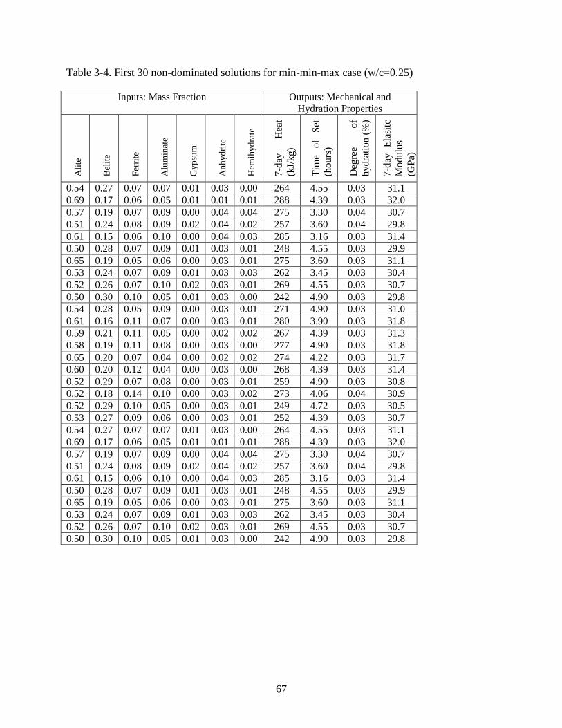
67
Table 3-4. First 30 non-dominated solutions for min-min-max case (w/c=0.25)
Inputs: Mass Fraction Outputs: Mechanical and
Hydration Properties
Ali
te
Bel
ite
Fer
rite
Alu
min
ate
Gy
psu
m
An
hy
dri
te
Hem
ihy
dra
te
7-d
ay
Hea
t
(kJ/
kg
)
Tim
e of
Set
(ho
urs
)
Deg
ree
of
hy
dra
tion
(%
)
7-d
ay
Ela
sitc
Mo
dulu
s
(GP
a)
0.54 0.27 0.07 0.07 0.01 0.03 0.00 264 4.55 0.03 31.1
0.69 0.17 0.06 0.05 0.01 0.01 0.01 288 4.39 0.03 32.0
0.57 0.19 0.07 0.09 0.00 0.04 0.04 275 3.30 0.04 30.7
0.51 0.24 0.08 0.09 0.02 0.04 0.02 257 3.60 0.04 29.8
0.61 0.15 0.06 0.10 0.00 0.04 0.03 285 3.16 0.03 31.4
0.50 0.28 0.07 0.09 0.01 0.03 0.01 248 4.55 0.03 29.9
0.65 0.19 0.05 0.06 0.00 0.03 0.01 275 3.60 0.03 31.1
0.53 0.24 0.07 0.09 0.01 0.03 0.03 262 3.45 0.03 30.4
0.52 0.26 0.07 0.10 0.02 0.03 0.01 269 4.55 0.03 30.7
0.50 0.30 0.10 0.05 0.01 0.03 0.00 242 4.90 0.03 29.8
0.54 0.28 0.05 0.09 0.00 0.03 0.01 271 4.90 0.03 31.0
0.61 0.16 0.11 0.07 0.00 0.03 0.01 280 3.90 0.03 31.8
0.59 0.21 0.11 0.05 0.00 0.02 0.02 267 4.39 0.03 31.3
0.58 0.19 0.11 0.08 0.00 0.03 0.00 277 4.90 0.03 31.8
0.65 0.20 0.07 0.04 0.00 0.02 0.02 274 4.22 0.03 31.7
0.60 0.20 0.12 0.04 0.00 0.03 0.00 268 4.39 0.03 31.4
0.52 0.29 0.07 0.08 0.00 0.03 0.01 259 4.90 0.03 30.8
0.52 0.18 0.14 0.10 0.00 0.03 0.02 273 4.06 0.04 30.9
0.52 0.29 0.10 0.05 0.00 0.03 0.01 249 4.72 0.03 30.5
0.53 0.27 0.09 0.06 0.00 0.03 0.01 252 4.39 0.03 30.7
0.54 0.27 0.07 0.07 0.01 0.03 0.00 264 4.55 0.03 31.1
0.69 0.17 0.06 0.05 0.01 0.01 0.01 288 4.39 0.03 32.0
0.57 0.19 0.07 0.09 0.00 0.04 0.04 275 3.30 0.04 30.7
0.51 0.24 0.08 0.09 0.02 0.04 0.02 257 3.60 0.04 29.8
0.61 0.15 0.06 0.10 0.00 0.04 0.03 285 3.16 0.03 31.4
0.50 0.28 0.07 0.09 0.01 0.03 0.01 248 4.55 0.03 29.9
0.65 0.19 0.05 0.06 0.00 0.03 0.01 275 3.60 0.03 31.1
0.53 0.24 0.07 0.09 0.01 0.03 0.03 262 3.45 0.03 30.4
0.52 0.26 0.07 0.10 0.02 0.03 0.01 269 4.55 0.03 30.7
0.50 0.30 0.10 0.05 0.01 0.03 0.00 242 4.90 0.03 29.8

68
Figure 3-1. Relationship between kiln temperature and C3S/C2S

69
Figure 3-2. Results of VCCTL simulations

70
Figure 3-3. Potential discrete combinations of cement and concrete

71
Figure 3-4. Elastic modulus vs. iteration with PSO

72
Figure 3-5. Distribution of cement phases for optimum with singe-objective PSO

73
Figure 3-6. Pareto fronts of four different bi-objective optimization scenarios without constraints
compared with the data envelope. Exploring the Pareto fronts with the PSO decreases
the computational cost by more than 70%

74
Figure 3-7. Comparison of PSO and GA of bi-objective optimization

75
Figure 3-8. 3D surface mesh of Pareto front from non-dominated solution (red dots) for the Min
(Time of set) – Min (C3S/C2S) – Max (E) case with different water-cement ratios. (a)
w/c=0.25; (b) w/c=0.33; (c) w/c=0.43; (d) w/c=0.53

76
Figure 3-9. (a) 3D surface mesh of Pareto front from non-dominated solution (red dots) for the
Max-Max-Max case (b) 3D surface mesh of Pareto front from non-dominated
solution (red dots) for the Min-Min-Min case, and (c) 3D surface of Pareto fronts for
the combined cases

77
Figure 3-10. Consolidation ratio and Improvement ratio for population size = 300

78
Figure 3-11. Convergence generation, number of simulations, number of optimal solutions vs.
population size

79
Figure 3-12. Process of deciding convex hull for evaluation cement data. (a) Finding convex
hull for Min (Time of set) – Min (C3S/C2S) – Min (E) case; (b) Finding convex hull
for Max (Time of set) – Max (C3S/C2S) – Max (E) case; (c)(d) Combined convex
hull. For cement data points close to Min (Time of set) – Min (C3S/C2S) – Min (E)
Pareto Front have higher score and those close to Max (Time of set) – Max (C3S/C2S)
– Max (E) Pareto Front have lower score

80
Figure 3-13. Marginal probability of non-exceedance with regard to time of set and heat proxy
for E ≥ 20 GPa cements. The score is defined as the 1-probability of non-exceedance
for the specified cement relative to all cement that meet the user specified constraints
(here the modulus). Scores of zero and unity represent the worst and best possible
outcomes

81
Figure 3-14. Different w/c with single cement chemistry on the marginal probability of non-
exceedance curve

82
Figure 3-15. Effect of w/c on scores with regard to time of set under single chemistry

83
Figure 3-16. Hermite and Beta distribution fitting for reduced data

84
Figure 3-17. Joint score of cement

85
CHAPTER 4
4 PHYSICAL-CHEMICAL MODELING OF A ROTARY CEMENT KILN
As introduced in Chapter 2, numerical models (C. Csernyei & Straatman, 2016; Martins
et al., 2002; Mastorakos et al., 1999; K. S. Mujumdar et al., 2006; Sadighi et al., 2011; Spang,
1972) exist to understand the behaviors of cement kilns, increase the cement production and
decrease the energy consumption and greenhouse gas emissions. To simulate reactions of the
rotary kiln and optimize the process and outputs, in this chapter, a physical-chemical one-
dimensional kiln model is developed based on knowledge of thermodynamics and clinker
chemistry from existing models. MATLAB R2016aTM solver ODE15s is used to solve an
ordinary partial differential equation system of the kiln model. The temperature profiles and
clinker species mass fractions are validated with the existing industrial kiln model and Bogue
calculation.
Although measuring data from operation cement plants is available at times, it is subject
to confidentiality and inherent limitations (C. M. Csernyei, 2016). The cement plant data such as
clinker production, energy cost, CO2 emissions is restricted to the precise operating parameters
that occurred at that time. Also, the majority of these parameters can only be estimated within a
certain degree of accuracy. Due to these reasons, research on the continued understanding of
cement rotary kilns is slow and heavily focused on computational modeling.
4.1 Model Validation
4.1.1 Solution Methodology
According to previous kiln models developed during the last 50 years, knowledge inside
the model is similar including the thermodynamics and clinker chemistry. However, the
approaches researchers used to solve the model are quite different. Some people developed their
own code with numerical methods (usually the fourth-order Runge-Kutta method) to solve for

86
the ODE/PDEs (C. Csernyei & Straatman, 2016; Martins et al., 2002; Spang, 1972), while others
used commercial software or open source numerical solves for their models (Darabi, 2007;
Guirao, Iglesias, Pistono, & Vázquez; Mastorakos et al., 1999; K. Mujumdar & Ranade, 2006;
Nørskov, 2012; Sadighi et al., 2011; Wang, Lu, Li, Li, & Hu, 2006).
For the current study, the kiln model Equations (2-1) – (2-29) are implanted into
Matlab2016aTM and the solver ODE15s is applied to solve the ODE system because of its high
computational efficiency and convenience in coupling with the optimization tool developed in
Chapter 3. By testing different ODE solvers including ODE45, ODE23, ODE15s, ODE23s,
ODE23t, ODE23tb in Matlab2016, ODE15s is more stable and performs better than other solvers
in solving stiff differential equations and dealing with singular matrix.
The procedure to solve for the computational kiln model is as follows:
1. An assumed temperature profile for the bed, gas, and shell was generated by assuming what
the temperatures may be throughout the kiln based on results from other researchers (C. M.
Csernyei, 2016; K. Mujumdar & Ranade, 2006). Based on Mujumdar and Csernyei’s model, a
linear profile for the gas temperature is generated in order to simplify the model. This profile was
generated using the inlet and outlet gas temperature, as well as an assumption for the temperature
and location of the peak gas temperature based on data received from the partner plant. The
initial temperature profile was obtained by using a tool called “Plot Digitizer” to digitize the
plots from papers. This tool allows users to pick the axis of a graph and choose the points on the
plot, then it generates a table of the x and y values (shown in Figure 4-1)
2. Internal heat transfer components were solved from Equation (2-1) to (2-10) excluding the
effects of clinker chemistry

87
3. ODE system (2-16) – (2-29) were solved for bed temperature and species mass fractions
through the use of Matlab2016a ODE15s solver. The bed temperature requirement for each
chemical reaction shown in Table 2-2 is taken into consideration
4. Shell temperature was solved using the heat balance Equation (2-29) by Newton-Raphson
method (Chapra & Canale, 1998)
5. A check was performed to see if the new temperature profiles of shell and solid bed were
within residual of 0.000001 of the previous profile
6. The new temperature profiles were passed back to the beginning of the model (step 2) and the
process repeated again till convergence
4.1.2 Results and Discussion
From the solution methodology in Section 4.3, the 1D physical-chemical kiln model
using Csernyei’s input (C. M. Csernyei, 2016) is solved after the iterative processes converge to
a solution for solid bed temperature and shell temperature. Mass fraction is plotted on the top of
Csernyei’s results. Bed height was taken as an adjustable factor for C3S at the exit of the kiln.
Red lines in Figure 4-2 show species mass fraction along the axial length of cement kiln without
adjusting bed height, which generate 20% more C3S compared with Csernyei’s result, shown
with black lines. Red lines in Figure 4-3 show the species mass fractions along the cement kiln
after adjusting the bed height from 0.75m to 0.58m. The mass fraction for each species matches
well with Csernyei’s results. Figure 4-4 shows the temperature profiles of solid bed, shell,
internal wall and freeboard gas along the kiln, which also matches well with Csernyei’s results.
Table 4-1 shows the comparison of inlet and outlet mass fraction of material compared to
the results of Bogue’s calculation (Bogue, 1929) and Csernyei’s prediction. From the clinker
mass fraction at the outlet of the kiln, the present prediction is close to Csernyei’s prediction
(1.24% difference), while has 15.89% difference compared to Bogue’s calculation. The reason

88
for the difference is Bogue’s calculation assumes entire amount input constituent are converted
into their species, which causes inherent error.
After comparison with Bogue’s calculation and Csernyei’s prediction, the present model
is verified with more published industrial data as well as some other researchers’ predictions (K.
Mujumdar & Ranade, 2006). Table 4-2 shows the comparison between the prediction of present
work with three cement plant data and Mujumdar’s prediction. From the outlet mass fraction, the
prediction of present work matches with published plant data very well.
4.2 Model Modification
4.2.1 CO2 Mass Fraction
The virtual cement plant kiln model in Chapter 2 calculated the mass fraction of each
solid component. Similarly, mass fraction of CO2 emissions from limestone decomposition could
be calculated with Equation (4-1).
𝑣𝑔𝑑𝑌𝐶𝑂2
𝑑𝑥=
𝐴𝑠
𝐴𝑔
𝜌𝑠
𝜌𝑔
𝑀𝐶𝑂2
𝑀𝐶𝑎𝑂𝑘1𝑌𝐶𝑎𝐶𝑂3 (4-1)
The mass fraction of CO2 emissions from limestone decomposition is shown in blue dash
line in Figure 4-5.
4.2.2 Raw Meal and Fuel Costs
First, the cost of raw material for cement plant was estimated and is provided in Table
4-3, which lists the unit price for cement raw material in the current market (sand and gravel
only). (https://www.statista.com/statistics/219381/sand-and-gravel-prices-in-the-us/).
By incorporating the unit price into VCP model based on the mass fraction of raw meal,
the relationship between 7-day modulus and raw meal cost was calculated (see Figure 4-6).
Modulus is observed to increase with the cost of raw meal, which is due to the increase of
limestone used as raw meal. From the linear regression fit for the data, a positive correlation

89
between gas peak temperature and modulus is obtained. That is because higher peak temperature
gives more alite, which plays an important role in cement strength development.
After the material cost is calculated, energy cost, or cost of fuel is considered. From
(Chatziaras et al., 2016), the average energy required to produce one ton of cement is 3.3 GJ,
which can be generated by 120 kg coal with a calorific value of 27.5 MJ/kg. Coal is the major
fuel used for cement production (Worrell et al., 2013). The cost of coal is $2.07/GJ
(https://www.statista.com/statistics/244479/us-consumer-price-estimates-for-coal-energy/).
Figure 4-7 shows the relationship between modulus and cost of fuel. Because of the linear
relation between energy and temperature, the cost of fuel has a linear relationship with
temperature.
Figure 4-8 shows the relationship between modulus and total cost by combining material
cost and fuel cost. Similar with Figure 4-6, modulus increases with total cost because of the
positive correlation between modulus and both cost. From Figure 4-8, energy cost accounts
about 30% of the total cost, which is verified by (Chatziaras et al., 2016).

90
Table 4-1. Species mass fractions model predictions compared with Bogue and Csernyei’s
prediction
Raw Meal at
inlet
Mass Fraction
from Csernyei’s
Work
Mass Fraction of
Present Work
CaCO3 0.3798 0.3798
CaO 0.3019 0.3019
SiO2 0.1594 0.1594
Al2O3 0.0246 0.0246
Fe2O3 0.0396 0.0396
Inert + Other 0.0947 0.0947
Clinker at the
Outlet
Mass Fraction
from Bogue’s
Calculation
Mass Fraction
from Csernyei’s
Work
Mass Fraction of
present work
C3S 0.582 0.546 0.546
C2S 0.130 0.049 0.041
C3A 0.063 0.027 0.027
C4AF 0.075 0.068 0.068
CaO 0.000 0.034 0.033
Summation 0.85 0.724 0.715

91
Table 4-2. Model predictions compared with industrial data and Mujumdar’s prediction
Industrial kiln 1 (2006) Industrial kiln 2 (2006) Industrial kiln 3 (2006)
Plant
Data
Mujumdar’s
Prediction
Present
Work
Plant
Data
Mujumdar’s
Prediction
Present
Work
Plant
Data
Mujumdar’s
Prediction
Present
Work
Inlet Mass Fraction
CaCO3 0.340 0.398 0.305
CaO 0.396 0.335 0.418
SiO2 0.179 0.185 0.190
Al2O3 0.0425 0.041 0.043
Fe2O3 0.0425 0.041 0.043
Initial
Temperature
of Solid, K
1123 1250 1025
Outlet Mass Fraction
C3S 0.483 0.508 0.489 0.508 0.502 0.503 0.500 0.504 0.506
C2S 0.239 0.222 0.202 0.257 0.263 0.209 0.269 0.249 0.222
C3A 0.051 0.051 0.048 0.048 0.051 0.048 0.042 0.052 0.048
C4AF 0.143 0.149 0.116 0.151 0.148 0.109 0.142 0.147 0.118
Residual
1.82%
2.38%
2.08%

92
Table 4-3. Unit price for raw material of cement plant
Raw material Chemical Composition Unit Price($/Ton)
Limestone CaCO3+CaO 15
Sand and Gravel SiO2 4.4
Clay Al2O3+Fe2O3 4

93
Figure 4-1. Digitization of the temperature plots from paper using “Plot Digitizer”

94
Figure 4-2. Species mass fractions along cement kiln without bed height adjustment compared
with published data

95
Figure 4-3. Species mass fractions along cement kiln with bed height adjustment compared with
published data

96
Figure 4-4. Temperature profiles in cement kiln from heat transfer.

97
Figure 4-5. Mass fraction of CO2 emissions from kiln model

98
Figure 4-6. Relationship between 7-day modulus (GPa) and cost of raw meal ($/Ton) under
different gas peak temperature

99
Figure 4-7. Relationship between 7-day modulus (GPa) and cost of fuel ($/Ton) under different
gas peak temperature

100
Figure 4-8. Relationship between 7-day modulus(GPa) and total cost under different gas peak
temperature

101
CHAPTER 5
5 OPTIMIZATION OF COUPLED VCP/VCCTL MODEL
This chapter introduces a coupled model which utilizes the VCP in combination with the
VCCTL to create a tool which models the production of Portland cement from the mine to the
point of placement. The coupling of VCP and VCCTL was performed to provide a tool that
couples cement production and hydration Portland cement. The model is a tool for the
optimization of raw material input, fuel, energy, emissions and cost for manufacture of Portland
cement in addition to the optimization of the physical properties of the resultant concrete.
5.1 Coupling VCP and VCCTL Modeling
5.1.1 Input Generation
Chapter 4 introduced 1D physical-chemical cement kiln model, which is considered as
virtual cement plant (VCP). In order to simulate the VCP, input files including the mass fraction
of raw meal, peak gas temperature and the location where peak gas temperature occurs within the
kiln are required.
The chemical composition of the raw meal at the inlet of cement kiln includes CaCO3,
CaO, SiO2, Al2O3, Fe2O3. It is common to use lime saturation factor (LSF), silica ratio (SR), and
alumina ratio (AR) in chemical analysis for cements, clinkers and phases instead of using oxide
components directly. The relationship between LSF, SR, AR and raw meal is as follows (Taylor,
1997):
Lime saturation factor (LSF) = CaO/(2.8SiO2+1.2Al2O3+0.65Fe2O3) (5-1)
Silica ratio (SR) = SiO2/(Al2O3+Fe2O3) (5-2)
Alumina ratio (AR) = Al2O3/Fe2O3 (5-3)
LSF is a ratio of CaO to other three oxide components, which control the ratio of
alite:belite produced within the cement kiln. The VCP model requires the mass fraction of raw

102
meal, calculated from Equations (5-1) – (5-3), where the LSR, SR, AR, Fe2O3, CaCO3/CaO are
considered as inputs which generate oxide components from the raw meal. According to Taylor,
the typical range for each ratio for the production of portland cement is as follows:
LSF - [0.9, 1.05]
SR - [2.0, 3.0]
AR - [0.8, 2.0]
Furthermore, the typical range of Fe2O3 content [0.01,0.1]. The CaCO3 to CaO ratio is
typically within a range of [40%,60%] and is directly obtained from the decarbonation of the
limestone through the kiln. Ultimately the mass fraction of the components, (CaCO3, CaO, SiO2,
Al2O3, Fe2O3) should be equal to 1. The inputs are generated utilizing two methods: a) fixed
intervals; b) uniformly distributed random numbers based on the ranges from each input.
Figure 5-1 and Figure 5-2 provide the distribution of 1956 inputs generated by fixed
intervals, where distributions of raw meal derived from Equation (5-1) – (5-3). The input was
generated from 100,000 individual samples, however, 1956 inputs or 1.96% satisfy the constraint
(components equal to 1). Figure 5-3 and Figure 5-4 show the distribution of inputs generated by
uniformly distributed random numbers from available sections and distribution of raw meal. The
number 200,000 individual samples were generated and only 1732 (0.87%) inputs satisfy the
constraint. The methodology used for the generation of different sample sizes (100,000 and
200,000) was done in an effort to acquire roughly the same number of inputs for each case (1956
and 1732). The fixed intervals (method a) did not provide a uniform distribution as shown in
figure 5-1; method b, the uniformly distributed random numbers were used to generate the inputs
for the coupled model.

103
Table 5-1 and Table 5-2 compare the VCP raw meal and clinker mass fraction with
different input generation approaches. The results of the two approaches are slightly different,
which is to be expected since different methods to generate inputs were used and provides
differences within the raw meal as well as cement clinker.
Taylor reported that the maximum LSF for modern cements is 1.02 and the range for LSF
(0.90 – 1.05) was borne from the use of a range slightly above the maximum reported. However,
the results obtained in Table 5-2, provide a low range of alite (18-48%), but is typically 40-70%
by mass (Stutzman, 2004). Subsequent to the production of the low values for alite, the model
was reproduced using the raw meal mass fractions from published industrial kiln data (C. M.
Csernyei, 2016; K. Mujumdar & Ranade, 2006) and are applied to determine the range of inputs.
After calculating LSF, AR, SR, Fe2O3 and CaCO3/CaO from Equation (5-1) – (5-3) using the
mass fractions of raw meal at inlet of the four industrial kilns (shown in Table 4-1 and Table
4-2), the ranges for material inputs is as follows: LSF [1.18, 1.36], SR [2.1, 2.5], AR [0.6, 1.0],
Fe2O3 [0.0396, 0.0430], CaCO3/CaO [42%, 56%].
Table 5-3 lists the expanded VCP input ranges combing Taylor’s work and information
from industrial kilns.
As introduced in Chapter 4, gas temperature profile is considered as input for the VCP
model, which contains the peak gas temperature and location of the peak gas temperature. Figure
5-5 gives an example of gas temperature as input profile for VCP. The peak gas temperature is
about 2100K, which happened at the point 0.84 of normalized kiln length away from entry of the
kiln. Based on other researchers’ gas profiles (C. M. Csernyei, 2016; K. Mujumdar & Ranade,
2006), peak gas temperature range is chosen as [1976, 2176] K and the range of location of peak
gas is chosen as [0.6, 0.9].

104
5.1.2 Input Range Testing
After the ranges for VCP inputs are established, cases with different range of material
input are analyzed. Table 5-4 shows the VCP results with different material input ranges. The
results are shown with regards to alite and belite mass fractions at different gas peak
temperatures. From Table 5-4, clinker mass fraction using Taylor’s material input range does not
cover enough searching space for the optimization tool. After expanding the input range by using
information from industrial kilns for VCP, alite space increases from [0.2, 0.45] to [0.2, 0.7] and
belite space increase from [0.25, 0.38] to [0, 0.38].
5.1.3 Schematic of coupled VCP-VCCTL model
In the following sections, the expanded inputs including 537 different kinds of chemistry,
10 different peak gas temperatures and 10 different locations of peak gas temperature are
considered for coupled VCP/VCCTL model. 53,700 inputs were ported to VCP, after 20 hours
running with Matlab2016a, 53,700 clinkers containing the information of mass fractions of
virtual clinker phases and related temperature profiles were created. The resultant “virtual
clinkers” phase chemistry and fineness are passed to VCCTL and run on UF HPC for virtual
cement initial microstructure reconstruction and hydration, as described in Chapter 2.
Subsequent to 6 days of run-time on the HPC, a series of output indicators with respect to the
performance for each virtual cement including time of set, 7-day mortar modulus, 7-day mortar
strength, 3-day heat are calculated.
5.1.4 Case Studies
Table 5-5 shows the results of coupled VCP-VCCTL with 53,700 inputs. Based on the
output of VCP, mass fractions of different cement clinker phases are plotted versus different
peak gas temperature and peak gas locations (also known as flame locations). For example, the
first plot in Table 5-5 shows alite mass fraction of virtual cements with 537 raw meal

105
combinations versus 10 peak gas temperatures. The results indicate that alite increases with the
peak gas temperature (or the highest temperature of flame inside the kiln), belite decreases with
the peak gas temperature, and CaO decreases with the peak gas temperature. The sensitivity of
clinker phases to temperature is increased when the flame is close to the exit of the kiln. That
means, if more alite is desired, one could move the flame position closer to the kiln exit, which
provides more of an influence than just increasing the peak gas temperature. Similarly, based on
the output of coupled VCP-VCCTL model, 7-day modulus and 3-day heat of hydration has a
similar trend with peak gas temperature and flame position, which matches with the results from
Figure 4-6. This case gives a meaningful guidance for the design of a cement kiln. Instead of
increasing the maximum temperature of flame inside the kiln to create a cement with higher
early strength, a simple position change of the flame is more energy efficient and sustainable.
5.2 Optimization of VCP-VCCTL Model
This section proposed an optimization tool for cement by applying PSO on coupled VCP-
VCCTL model to save material cost, energy consumption, and decrease CO2 emissions.
5.2.1 Cost vs. Modulus
The production of cement typically involves two major costs: energy and materials. The
cost of energy is reported to represent a total of 20-40% of the total cost (Chatziaras et al., 2016;
Worrell et al., 2013).
Multi-objective PSO was integrated into the coupled VCP-VCCTL model to create an
integrated computational optimization VCP-VCCTL tool for energy saving, cost saving and
greenhouse gas emissions reduction without sacrificing cement productivity and performance.
Similar to Chapter 3, Pareto fronts of four different bi-objective scenarios are plotted in Figure
5-7 to show clear trade-off between modulus and material cost.

106
In Figure 5-7, the Min (cost of raw meal)-Max (E) Pareto front is what the cement
industry wants. To preserve strength, the cost cannot be reduced too much from 24.7 to 24.1
$/Ton (2.43% savings). From the Min-Max Pareto front, some moduli have to be sacrificed if
less cost is required. Most of the cement in Figure 5-7 is cheaper and weaker.
5.2.2 CO2 Emissions vs. Modulus
As introduced in Chapter 2, 50% of the total emissions comes from calcination/
decomposition of limestone inside the cement kiln, which is a considerable amount of emissions.
Reduction of CO2 emissions from limestone is taken into consideration in this section.
In order to reduce CO2 emissions without sacrificing cement strength, CO2 emissions
from limestone and 7-day modulus are considered as the objectives in PSO at the same time.
Figure 5-8 shows the four Pareto fronts for different optimization scenarios on E vs. CO2
emissions from limestone decomposition. In Figure 5-8, the Min(CO2 emssion)-Max(E) Pareto
front is what the cement industry wants. The point with 0.14 CO2 emissions and 27.8 GPa is the
optimal cement. When mass fraction of CO2 emissions is more than 0.14, most of the cement
give more emissions without sacrificing too much strength. More alite means more
decomposition, which typically gives more strength. The results of this optimization suggest the
coupled VCP/VCCTL model could be used as a tool to optimize for a design cement.
5.2.3 Cost vs. CO2 Emissions vs. Modulus
Figure 5-9 shows the Pareto front for Min(cost)-Min(CO2 emssions)-Max(E), which is
what the cement industry wants. From the Pareto front, producing cements with high modulus
cost more money and release more CO2 emissions. If the cost of raw meal is reduced from 12.4
$/ton to 11.4 $/ton (9% reduction) and the mass fraction of CO2 emissions is reduced from 0.16
to 0.14 (15% reduction), modulus would be reduced from 26GPa to 22GPa (18% reduction).
This information could be used for make the decision based on the weight of strength, economy

107
and sustainability. For example, if it is acceptable to sacrifice 18% strength for a cement
company, both the sustainability and economic value would improve a lot.

108
Table 5-1. Comparison of VCP raw meal mass fraction from different input generation
approaches
Lower Bound Upper Bound Mean Value
Fixed
Interval
Uniformly
Distributed
Fixed
Interval
Uniformly
Distributed
Fixed
Interval
Uniformly
Distributed
CaCO3 0.2645 0.2666 0.4288 0.4258 0.3440 0.3424
CaO 0.2645 0.2665 0.4288 0.4250 0.3440 0.3457
SiO2 0.1997 0.2014 0.2447 0.2433 0.2211 0.2216
Al2O3 0.0342 0.0337 0.0691 0.0740 0.0512 0.0512
Fe2O3 0.0264 0.0247 0.0591 0.0599 0.0398 0.0394

109
Table 5-2. Comparison of VCP clinker mass fraction from different input generation approaches
From fixed interval inputs From random inputs
Lower
bound
Upper
bound
Mean
Value
Lower
bound
Upper
bound
Mean
Value
C3S 0.1890 0.4822 0.2998 0.1953 0.4574 0.3028
C2S 0.2330 0.3972 0.3343 0.2445 0.3917 0.3360
C3A 0.0406 0.1268 0.0797 0.0412 0.1149 0.0725
C4AF 0.0691 0.1405 0.0989 0.0712 0.1360 0.1008

110
Table 5-3. Expanded VCP material input ranges combing Taylor’s ranges and ranges of
industrial kilns
VCP Material
Input Taylor’s range
Range of
Industrial Kilns
Gap Range
between Taylor
and Industrial
Kilns
Expanded Range
LSF [0.9, 1.05] [1.18, 1.36] [1.05,1.18] [0.9,1.36]
SR [2.0, 3.0] [2.1, 2.5] [2.1,2.5] [2.0,3.0]
AR [0.8, 2.0] [0.6, 1.0] [0.6,1.0] [0.6,2.0]
Fe2O3 [0.01,0.1] [0.0396, 0.0430] [0.0396,0.0430] [0.01,0.1]
CaCO3/CaO [40%, 60%] [42%, 56%] [42%,56%] [40%,60%]

111
Table 5-4. Comparison of VCP cases with different material input range
543 Chemistry
(537 Taylor’s Range + 4
Industrial Kiln Range)
561 Chemistry (Industrial
Kiln Range)
366 Chemistry
(Gap Range)
537 Chemistry
(Expanded Range)
C3S
vs.
Tg_peak
C3S
vs.
Tg_peak
(Box
Plot)
C2S
vs.
Tg_peak

112
Table 5-4. Continued
543 Chemistry
(537 Taylor’s Range + 4
Industrial Kiln Range)
561 Chemistry (Industrial
Kiln Range)
366 Chemistry
(Gap Range)
537 Chemistry
(Expanded Range)
C2S
vs.
Tg_peak
(Box
Plot)

113
Table 5-5. Coupled VCP-VCCTL results with 53,700 inputs
Lg_peak=0.6 Lg_peak=0.7 Lg_peak=0.8 Lg_peak=0.9
C3S vs.
Tg_peak
C3S vs.
Tg_peak
(Box
Plot)
C2S vs.
Tg_peak
C2S vs.
Tg_peak
(Box
Plot)

114
Table 5-5. Continued
Lg_peak=0.6 Lg_peak=0.7 Lg_peak=0.8 Lg_peak=0.9
CaO vs.
Tg_peak
CaO vs.
Tg_peak
(Box
Plot)
7-day
modulus
vs.
Tg_peak
7-day
modulus
vs.
Tg_peak
(box
plot)

115
Table 5-5. Continued
Lg_peak=0.6 Lg_peak=0.7 Lg_peak=0.8 Lg_peak=0.9
3-day
heat vs.
Tg_peak
3-day
heat vs.
Tg_peak
(box
plot)

116
Figure 5-1. Distribution of inputs for VCP generated from fixed intervals

117
Figure 5-2. Distribution of raw meals derived from fixed interval inputs of VCP

118
Figure 5-3. Distribution of input for VCP generated from uniformly distributed inputs

119
Figure 5-4. Distribution of raw meals derived from uniformly distributed inputs of VCP

120
Figure 5-5. Example of gas temperature input profile for VCP

121
Figure 5-6. Flow of coupled VCP-VCCTL model

122
Figure 5-7. Pareto fronts of four different bi-objective optimization scenarios on E vs. cost of
raw meal compared with the data envelope

123
Figure 5-8. Pareto fronts of four different bi-objective optimization scenarios on E vs. CO2
emissions from limestone compared with the data envelope

124
Figure 5-9. Pareto fronts of tri-objective optimization scenarios on E vs. CO2 emissions from
limestone vs. cost

125
CHAPTER 6
6 CONCLUSIONS AND RECOMMENDATIONS
In summary, the completed research work to date focuses on the metaheuristic algorithms
applied to virtual cement and cement plant modeling. Single-objective and multi-objective
optimizations with PSO and GA are applied to a set of sample cement data from VCCTL. A
scoring system is created to evaluate cement based on Pareto front optimization results. A 1D
physical-chemical cement rotary kiln model is simulated with Matlab2016a solver and integrated
with VCCTL and multi-objective metaheuristic algorithm on the HiperGator high performance
computing cluster at University of Florida. A computational framework simulating cement and
cement plant intelligently based on users’ requirements and guiding the optimal designs is
proposed.
The integrated model in this dissertation could provide a quantitative optimization tool
for different energy efficiency measures addressed from cement plants and reduce energy,
material consumption and greenhouse gas emissions without losing the performance of material.
However, there is some limitations of the computational framework including lack of
criterion for detecting unrealistic virtual testing data. Currently, user-defined range of input is
given to VCP-VCCTL model to conduct optimization. For the future work, threshold could be
introduced into the model to detect unrealistic cases. Another challenge of this model is it needs
more experiment data from cement plant to validate the accuracy of the model. Also, the model
could be less computationally expensive with more efficient approaches within the coupling and
the algorithm.

126
LIST OF REFERENCES
Aarts, E. H., & Korst, J. H. (1988). Simulated annealing. ISSUES, 1, 16.
Ahmad, S., & Alghamdi, S. A. (2014). A statistical approach to optimizing concrete mixture
design. The Scientific World Journal, 2014.
Aı̈tcin, P.-C. (2000). Cements of yesterday and today: concrete of tomorrow. Cement and
Concrete research, 30(9), 1349-1359.
Akhtar, S. S., Ervin, E., Raza, S., & Abbas, T. (2013). From coal to natural gas: Its impact on
kiln production, Clinker quality and emissions. Paper presented at the Cement Industry
Technical Conference (CIC), 2013 IEEE-IAS/PCA.
Arrhenius, S. (1889). Über die Reaktionsgeschwindigkeit bei der Inversion von Rohrzucker
durch Säuren. Zeitschrift für physikalische Chemie, 4(1), 226-248.
Atmaca, A., & Yumrutaş, R. (2014). Analysis of the parameters affecting energy consumption of
a rotary kiln in cement industry. Applied Thermal Engineering, 66(1), 435-444.
Babushkin, V. I., Matveev, G. M., & Mchedlov-Petrosi︠a︡n, O. P. (1985). Thermodynamics of
silicates: Springer.
Barr, P. V. (1986). Heat transfer processes in rotary kilns. University of British Columbia.
Benhelal, E., Zahedi, G., Shamsaei, E., & Bahadori, A. (2013). Global strategies and potentials
to curb CO 2 emissions in cement industry. Journal of cleaner production, 51, 142-161.
Bentz, D. P. (1997). Three‐Dimensional Computer Simulation of Portland Cement Hydration
and Microstructure Development. Journal of the American Ceramic Society, 80(1), 3-21.
Bentz, D. P., Feng, X., & Stutzman, P. E. (2000). Analysis of CCRL proficiency cements 135 and
136 using CEMHYD3D: National Institute of Standards and Technology, Technology
Administration, US Department of Commerce.
Bickley, J. A., Hooton, R. D., & Hover, K. C. (2006). Performance specifications for durable
concrete. Concrete international, 28(09), 51-57.
Bićanić, N., De Borst, R., Mang, H., & Meschke, G. (2003). Computational modelling of
concrete structures. Paper presented at the Proc. of the EURO-C Conference.
Bogue, R. H. (1929). Calculation of the compounds in Portland cement. Industrial &
Engineering Chemistry Analytical Edition, 1(4), 192-197.
Bonnans, J.-F., Gilbert, J. C., Lemaréchal, C., & Sagastizábal, C. A. (2006). Numerical
optimization: theoretical and practical aspects: Springer Science & Business Media.

127
Bremermann, H. J. (1958). The evolution of intelligence: The nervous system as a model of its
environment: University of Washington, Department of Mathematics.
Bullard, J. W. (2014). Virtual Cement and Concrete Testing Laboratory: Version 9.5 User Guide.
Bullard, J. W., Ferraris, C., Garboczi, E. J., Martys, N., & Stutzman, P. (2004). Virtual cement.
Chapt, 10, 1311-1331.
Bullard, J. W., & Stutzman, P. E. (2006). Analysis of CCRL proficiency cements 151 and 152
using the virtual cement and concrete testing laboratory. Cement and Concrete Research,
36(8), 1548-1555.
Burke, E. K., & Kendall, G. (2005). Search methodologies: Springer.
Cement, A. ASTM C150, Type I-Normal Portland type. 1. Acquire all cement for entire project
from same source.
Chapra, S. C., & Canale, R. P. (1998). Numerical methods for engineers (Vol. 2): McGraw-Hill
New York.
Chatziaras, N., Psomopoulos, C. S., & Themelis, N. J. (2016). Use of waste derived fuels in
cement industry: a review. Management of Environmental Quality: An International
Journal, 27(2), 178-193.
Chen, Y., & Odler, I. (1992). On the origin of Portland cement setting. Cement and Concrete
Research, 22(6), 1130-1140.
Collins, N., Eglese, R., & Golden, B. (1988). Simulated annealing–an annotated bibliography.
American Journal of Mathematical and Management Sciences, 8(3-4), 209-307.
Csernyei, C., & Straatman, A. G. (2016). Numerical modeling of a rotary cement kiln with
improvements to shell cooling. International Journal of Heat and Mass Transfer, 102,
610-621.
Csernyei, C. M. (2016). Numerical Modelling of a Rotary Cement Kiln with External Shell
Cooling Fans. The University of Western Ontario.
Damtoft, J. S., Lukasik, J., Herfort, D., Sorrentino, D., & Gartner, E. M. (2008). Sustainable
development and climate change initiatives. Cement and concrete research, 38(2), 115-
127.
Darabi, P. (2007). A mathematical model for cement kilns. University of British Columbia.
Deb, K., Pratap, A., Agarwal, S., & Meyarivan, T. (2002). A fast and elitist multiobjective
genetic algorithm: NSGA-II. IEEE transactions on evolutionary computation, 6(2), 182-
197.

128
Eberhart, R., & Kennedy, J. (1995). A new optimizer using particle swarm theory. Paper
presented at the Micro Machine and Human Science, 1995. MHS'95., Proceedings of the
Sixth International Symposium on.
Fraser, A. S. (1957). Simulation of genetic systems by automatic digital computers ii. effects of
linkage on rates of advance under selection. Australian Journal of Biological Sciences,
10(4), 492-500.
Garboczi, E. J., & Bentz, D. P. (1995). Multi-scale picture of concrete and its transport
properties: introduction for non-cement researchers: National Institute of Standards and
Technology.
Garboczi, E. J., & Bentz, D. P. (2001). The effect of statistical fluctuation, finite size error, and
digital resolution on the phase percolation and transport properties of the NIST cement
hydration model. Cement and Concrete Research, 31(10), 1501-1514.
Garboczi, E. J., & Berryman, J. G. (2001). Elastic moduli of a material containing composite
inclusions: effective medium theory and finite element computations. Mechanics of
Materials, 33(8), 455-470.
Garboczi, E. J., Bullard, J. W., & Bentz, D. P. (2004). Virtual testing of cement and concrete—
USA 2004. Concrete international, 26(12), 33-37.
Geem, Z. W., Kim, J. H., & Loganathan, G. (2001). A new heuristic optimization algorithm:
harmony search. Simulation, 76(2), 60-68.
Ghezal, A., & Khayat, K. H. (2002). Optimizing self-consolidating concrete with limestone filler
by using statistical factorial design methods. ACI Materials Journal, 99(3), 264-272.
Glover, F., & Laguna, M. (2013). Tabu Search∗: Springer.
Goel, T., & Stander, N. (2010). A Study of the Convergence Characteristics of Multiobjective
Evolutionary Algorithms. Paper presented at the 13th AIAA/ISSMO Multidisciplinary
Analysis Optimization Conference.
Goldberg, D. E., & Samtani, M. P. (1986). Engineering optimization via genetic algorithm.
Paper presented at the Electronic Computation:.
Grosan, C., Abraham, A., & Chis, M. (2006). Swarm intelligence in data mining. Swarm
Intelligence in Data Mining, 1-20.
Guirao, J., Iglesias, S., Pistono, J., & Vázquez, R. Model of Mass and Energy Transfer in a
Clinker Rotary Kiln.
Haecker, C., Bentz, D., Feng, X., & Stutzman, P. (2003). Prediction of cement physical
properties by virtual testing. Cement International, 1(3), 86-92.

129
Haecker, C.-J., Garboczi, E., Bullard, J., Bohn, R., Sun, Z., Shah, S., et al. (2005). Modeling the
linear elastic properties of Portland cement paste. Cement and Concrete Research, 35(10),
1948-1960.
Hain, M., & Wriggers, P. (2008). Numerical homogenization of hardened cement paste.
Computational Mechanics, 42(2), 197-212.
Holland, J. H. (1975). Adaptation in natural and artificial systems. An introductory analysis with
application to biology, control, and artificial intelligence. Ann Arbor, MI: University of
Michigan Press.
Holland, J. H. (1992). Adaptation in natural and artificial systems: an introductory analysis with
applications to biology, control, and artificial intelligence: MIT press.
Hottel, H., & Sarofim, A. (1965). Radiative transport. McCravv Hill, New York.
Hu, X., Eberhart, R. C., & Shi, Y. (2003). Engineering optimization with particle swarm. Paper
presented at the Swarm Intelligence Symposium, 2003. SIS'03. Proceedings of the 2003
IEEE.
Jaumard, B., OW, P. S., & Simeone, B. (1988). A selected artificial intelligence bibliography for
operations researchers. Annals of Operations Research, 12(1), 1-50.
Kabir, G., Abubakar, A., & El-Nafaty, U. (2010). Energy audit and conservation opportunities
for pyroprocessing unit of a typical dry process cement plant. Energy, 35(3), 1237-1243.
Kaige, S., Murata, T., & Ishibuchi, H. (2003). Performance evaluation of memetic EMO
algorithms using dominance relation-based replacement rules on MOO test problems.
Paper presented at the Systems, Man and Cybernetics, 2003. IEEE International
Conference on.
Kirkpatrick, S. (1984). Optimization by simulated annealing: Quantitative studies. Journal of
statistical physics, 34(5), 975-986.
Lagergren, E. S., Snyder, K. A., & Simon, M. J. (1997). Concrete Mixture Optimization Using
Statistical Mixture Design Methods.
Li, G., Goel, T., & Stander, N. (2008). Assessing the convergence properties of NSGA-II for
direct crashworthiness optimization. Paper presented at the 10th International LS-
DYNA® User’s Conference, Detroit MI.
Li, L., Huang, Z., & Liu, F. (2009). A heuristic particle swarm optimization method for truss
structures with discrete variables. Computers & Structures, 87(7), 435-443.
Li, L., Huang, Z., Liu, F., & Wu, Q. (2007). A heuristic particle swarm optimizer for
optimization of pin connected structures. Computers & Structures, 85(7), 340-349.

130
Li, S. Q., Ma, L. B., Wan, W., & Yao, Q. (2005). A Mathematical Model of Heat Transfer in a
Rotary Kiln Thermo‐Reactor. Chemical engineering & technology, 28(12), 1480-1489.
Mamlouk, M. S., & Zaniewski, J. P. (1999). Materials for civil and construction engineers:
Addison-Wesley Reading, Mass, USA.
Martins, M. A., Oliveira, L. S., & Franca, A. S. (2002). Modeling and simulation of limestone
calcinations in rotary kilns. ZKG International, 55(4), 76-87.
Martí, L., García, J., Berlanga, A., & Molina, J. M. (2007). A cumulative evidential stopping
criterion for multiobjective optimization evolutionary algorithms. Paper presented at the
Proceedings of the 9th annual conference companion on Genetic and evolutionary
computation.
Mastorakos, E., Massias, A., Tsakiroglou, C., Goussis, D., Burganos, V., & Payatakes, A. (1999).
CFD predictions for cement kilns including flame modelling, heat transfer and clinker
chemistry. Applied Mathematical Modelling, 23(1), 55-76.
Mindess, S., & Young, J. (1981). Concrete. Englewood: NJ, Prentice Hall.
Mujumdar, K., & Ranade, V. (2006). Simulation of rotary cement kilns using a one-dimensional
model. Chemical Engineering Research and Design, 84(3), 165-177.
Mujumdar, K. S., Arora, A., & Ranade, V. V. (2006). Modeling of rotary cement kilns:
applications to reduction in energy consumption. Industrial & engineering chemistry
research, 45(7), 2315-2330.
Mujumdar, K. S., Ganesh, K., Kulkarni, S. B., & Ranade, V. V. (2007). Rotary Cement Kiln
Simulator (RoCKS): Integrated modeling of pre-heater, calciner, kiln and clinker cooler.
Chemical Engineering Science, 62(9), 2590-2607.
Muthukumar, M., & Mohan, D. (2004). Optimization of mechanical properties of polymer
concrete and mix design recommendation based on design of experiments. Journal of
applied polymer science, 94(3), 1107-1116.
Neville, A. M. (1995). Properties of concrete.
Nissen, V. (1993). Evolutionary algorithms in management science: An overview and list of
references: European Study Group for Evolutionary Economics.
Noshirvani, G., Shirvani, M., Askari-Mamani, J., & Nourzadeh, H. (2013). Estimation of coating
thickness in a rotary kiln by using shell temperature and kiln modeling. ZKG
international(11), 58-71.
Nørskov, L. K. (2012). Combustion of solid alternative fuels in the cement kiln burner. Technical
University of Denmark.

131
Odelson, J. B., Kerr, E. A., & Vichit-Vadakan, W. (2007). Young's modulus of cement paste at
elevated temperatures. Cement and Concrete Research, 37(2), 258-263.
Odler, I. (1998). Hydration, setting and hardening of Portland cement. LEA’s Chemistry of
Cement and Concrete, 4, 241-297.
Osman, I. H. (1995). An introduction to meta-heuristics. Operational Research Tutorial Papers,
92-122.
Osman, I. H., & Laporte, G. (1996). Metaheuristics: A bibliography: Springer.
Parsopoulos, K. E., & Vrahatis, M. N. (2002). Recent approaches to global optimization
problems through particle swarm optimization. Natural computing, 1(2-3), 235-306.
Patel, R., Hossain, K., Shehata, M., Bouzoubaa, N., & Lachemi, M. (2004). Development of
statistical models for mixture design of high-volume fly ash self-consolidating concrete.
Materials Journal, 101(4), 294-302.
Peray, K. E., & Waddell, J. J. (1986). The rotary cement kiln: Edward Arnold.
Pirlot, M. (1992). General local search heuristics in combinatorial optimization: a tutorial.
Belgian Journal of Operations Research, Statistics and Computer Science, 32(1-2), 7-69.
Press, W. H., Teukolsky, S. A., Vetterling, W. T., & Flannery, B. P. (2007). Numerical recipes:
the art of scientific computing: Cambridge University Press, New York.
Rajeev, S., & Krishnamoorthy, C. (1992). Discrete optimization of structures using genetic
algorithms. Journal of structural engineering, 118(5), 1233-1250.
Rayward-Smith, V. J., Osman, C., Reeves, C. R., & Smith, G. D. (1996). Modern heuristic
search methods: John Wiley.
Reddy, B. V., & Jagadish, K. (2003). Embodied energy of common and alternative building
materials and technologies. Energy and buildings, 35(2), 129-137.
Reddy, B. V., Leuzinger, G., & Sreeram, V. (2014). Low embodied energy cement stabilised
rammed earth building—A case study. Energy and Buildings, 68, 541-546.
Romeo, L. M., Catalina, D., Lisbona, P., Lara, Y., & Martínez, A. (2011). Reduction of
greenhouse gas emissions by integration of cement plants, power plants, and CO2 capture
systems. Greenhouse Gases: Science and Technology, 1(1), 72-82.
Roudenko, O., & Schoenauer, M. (2004). A steady performance stopping criterion for Pareto-
based evolutionary algorithms.
Sadighi, S., Shirvani, M., & Ahmad, A. (2011). Rotary cement kiln coating estimator: Integrated
modelling of kiln with shell temperature measurement. The Canadian Journal of
Chemical Engineering, 89(1), 116-125.

132
Saidur, R., Hossain, M., Islam, M., Fayaz, H., & Mohammed, H. (2011). A review on kiln
system modeling. Renewable and Sustainable Energy Reviews, 15(5), 2487-2500.
Sharda, R. (1994). Neural networks for the MS/OR analyst: An application bibliography.
Interfaces, 24(2), 116-130.
Shetty, M. (2005). Concrete technology: publisher not identified.
Shi, Y. (2001). Particle swarm optimization: developments, applications and resources. Paper
presented at the evolutionary computation, 2001. Proceedings of the 2001 Congress on.
Simon, M. (2003). Concrete mixture optimization using statistical methods: final report: US
Department of Transportation, Federal Highway Administration, Research, Development
and Technology, Turner-Fairbank Highway Research Center.
Simon, M., Snyder, K., & Frohnsdorff, G. (1999). Advances in concrete mixture optimization.
Paper presented at the Proceedings of International Congress on Creating with Concrete
University of Dundee,(ed. Dhir & McCarthy) pp.
Sonebi, M., & Bassuoni, M. (2013). Investigating the effect of mixture design parameters on
pervious concrete by statistical modelling. Construction and Building Materials, 38, 147-
154.
Soudki, K., El-Salakawy, E., & Elkum, N. (2001). Full factorial optimization of concrete mix
design for hot climates. Journal of materials in civil engineering, 13(6), 427-433.
Spang, H. (1972). A dynamic model of a cement kiln. Automatica, 8(3), 309-323.
Stadler, K. S., Poland, J., & Gallestey, E. (2011). Model predictive control of a rotary cement
kiln. Control Engineering Practice, 19(1), 1-9.
Standard, A. D245, 2006,“Standard Practice for Establishing Structural Grades and Related
Allowable Properties for Visually Graded Lumber,” ASTM International, West
Conshohocken, PA. ASTM D245, 6.
Stewart, B. S., Liaw, C.-F., & White, C. C. (1994). A bibliography of heuristic search research
through 1992. IEEE transactions on Systems, Man, and Cybernetics, 24(2), 268-293.
Stutzman, P. (2004). Scanning electron microscopy imaging of hydraulic cement microstructure.
Cement and Concrete Composites, 26(8), 957-966.
Tan, O., Zaimoglu, A. S., Hinislioglu, S., & Altun, S. (2005). Taguchi approach for optimization
of the bleeding on cement-based grouts. Tunnelling and underground space technology,
20(2), 167-173.
Taylor, H. F. (1997). Cement chemistry: Thomas Telford.

133
Thomas, J. J., Biernacki, J. J., Bullard, J. W., Bishnoi, S., Dolado, J. S., Scherer, G. W., et al.
(2011). Modeling and simulation of cement hydration kinetics and microstructure
development. Cement and Concrete Research, 41(12), 1257-1278.
Trautmann, H., Ligges, U., Mehnen, J., & Preuss, M. (2008). A convergence criterion for
multiobjective evolutionary algorithms based on systematic statistical testing. Paper
presented at the International Conference on Parallel Problem Solving from Nature.
Tscheng, S., & Watkinson, A. (1979). Convective heat transfer in a rotary kiln. The Canadian
Journal of Chemical Engineering, 57(4), 433-443.
Vallgårda, A., & Redström, J. (2007). Computational composites. Paper presented at the
Proceedings of the SIGCHI conference on Human factors in computing systems.
Voß, S., Martello, S., Osman, I. H., & Roucairol, C. (2012). Meta-heuristics: Advances and
trends in local search paradigms for optimization: Springer Science & Business Media.
Wang, S., Lu, J., Li, W., Li, J., & Hu, Z. (2006). Modeling of pulverized coal combustion in
cement rotary kiln. Energy & Fuels, 20(6), 2350-2356.
Watts, B. E. (2013). Analysis of the Sensitivity of a Concrete Virtual Model to Different
Material Input Parameters.
Worrell, E., Kermeli, K., & Galitsky, C. (2013). Energy Efficiency Improvement and Cost
Saving Opportunities for Cement Making An ENERGY STAR® Guide for Energy and
Plant Managers: EPA-United States Environmental Protection Agency.
Wu, S.-J., & Chow, P.-T. (1995). Steady-state genetic algorithms for discrete optimization of
trusses. Computers & Structures, 56(6), 979-991.
Xiaoyong, L., & Wendi, M. (2011). Optimization for mix design of high-performance concrete
using orthogonal test. Innovative Computing and Information, 364-372.
Yang, L., Gurley, K. R., & Prevatt, D. O. (2013). Probabilistic modeling of wind pressure on
low-rise buildings. Journal of Wind Engineering and Industrial Aerodynamics, 114, 18-
26.
Zhang, Y., Cao, S.-X., Shao, S., Chen, Y., Liu, S.-L., & Zhang, S.-S. (2011). Aspen Plus-based
simulation of a cement calciner and optimization analysis of air pollutants emission.
Clean Technologies and Environmental Policy, 13(3), 459-468.
Zitzler, E., Thiele, L., Laumanns, M., Fonseca, C. M., & Da Fonseca, V. G. (2003). Performance
assessment of multiobjective optimizers: An analysis and review. IEEE Transactions on
evolutionary computation, 7(2), 117-132.

134
BIOGRAPHICAL SKETCH
Chengcheng Tao was born in Wuhu, Anhui Province, China. In June 2011, she received
her bachelor’s degree with highest honor in civil engineering from Shanghai Normal University,
China. Then, she received her master’s degree in civil engineering from Carnegie Mellon
University in May, 2012 and master’s degree in mechanical engineering from Johns Hopkins
University in August, 2014. Her master’s thesis topic was “Crystal plasticity based finite element
modeling in polycrystalline ti-7al alloys”. In August 2014, she was accepted into the Ph.D.
program in the Department of Civil and Coastal Engineering at the University of Florida with a
focus on optimization in cement and concrete and cement plant modeling under the guidance of
Dr. Forrest Masters and Dr. Christopher Ferraro.