© 2016 Jayant Ahalawat

DATA DRIVEN MODELING OF CORN YIELD: A MACHINE LEARNING APPROACH

BY

JAYANT AHALAWAT

THESIS

Submitted in partial fulfillment of the requirements for the degree of Master of Science in Civil Engineering

in the Graduate College of the University of Illinois at Urbana-Champaign, 2016

Urbana, Illinois Adviser: Professor Barbara Minsker

ii

ABSTRACT With the increase in global population and growing demand for food, there has been considerable

research in leveraging data in the agricultural domain to improve yields. Tremendous amounts of

data are generated on farms, ranging from amount of water used for irrigation to the quantities

of fertilizers applied. To our knowledge, this study is the first that uses high-resolution crop data

(280,000 points at 10-meter scale) to improve understanding and prediction of the impact of

hydrology-related variables, namely topography, soil, and weather, on yield.

Supervised machine learning techniques, namely decision trees and random forests, are

used to develop data-driven predictive models. A case study of corn fields in Iowa demonstrates

how an ensemble technique like random forest can improve upon simpler models like decision

trees. In addition, the random forest model is used to develop partial dependence plots of corn

yield versus different feature variables (derived from topography, soil and weather). These plots

help in understanding how yield varies with changes in different feature variables. For example,

there is an optimum topographic range in which yield is high. Corn yield is higher in gentle

depressions as compared to steep slopes and very deep depressions. Further, very high and very

low precipitation during the emergence stage (VE) is most likely to lead to lower yield.

The model described in this study can also be used to develop intra-field importance maps

that delineate importance of a particular type of a variable (like precipitation) on corn yield at

fine scales. These maps can be used to visually inspect the interaction of topography and

precipitation and the resultant impact on corn yield, and could be used to support more fine-scale

farm management strategies (e.g., irrigation only where needed).

iii

   

 

 

 

 

 

 

 

 

 

 

 

 

 

To Mom, Dad and Arushi

 

 

iv

Acknowledgements At the outset, I would like to thank my adviser, Professor Barbara Minsker, for giving me

the opportunity to work on this project. Working with her has been quite a wonderful

and educational experience. She has been a constant source of support and guidance

throughout the two years of my graduate studies. I am truly glad to have her as a mentor

in my life.

I am grateful to Professor Praveen Kumar for his insightful comments which helped in

shaping this research into its current form.

I would also like to thank folks from John Deere’s Technological Innovation Center

(JDTIC), for not only providing the data and funding for this project but also giving me

access to their offices at the research park. I would especially like to thank Kevin

Armstrong for his suggestions and advice throughout the course of this project.

I am truly blessed to have amazing friends in my life. To Ojaswi, Lakshmi and Nidhi – I

thank all of you for always being there for me. I would also like to thank my flat mates,

Arko and Neetesh, for bearing with me and providing much needed diversions from

graduate school.

I would like to express my deepest gratitude to my parents and siblings for being a

constant source of support and encouragement throughout my life.

Finally, to Arushi, I thank you for your love and support and making the last two years

as wonderful as they could be.

v

Table of Contents 1. Introduction .................................................................................................................. 1

2. Methods ........................................................................................................................ 4

2.1 Feature Engineering ................................................................................................ 6

2.1.1 Topography ....................................................................................................... 6

2.1.2 Soil ..................................................................................................................... 9

2.1.3 Weather ............................................................................................................. 9

2.1.4 Planting Date .................................................................................................. 12

2.2 Machine Learning Models ...................................................................................... 13

2.2.1 Decision Trees ................................................................................................. 13

2.2.2 Random Forests ............................................................................................... 15

3. Case Study .................................................................................................................. 17

3.1 Description of Data and Machine Learning Models ............................................... 17

3.2 Results and Discussion .......................................................................................... 20

3.2.1 Comparison of Random Forest and Decision Tree .......................................... 20

3.2.2 Variable Importance ........................................................................................ 22

3.2.3 Partial Dependence .......................................................................................... 25

4. Discussion and Conclusions ........................................................................................ 35

References ....................................................................................................................... 38

  1

Chapter 1

Introduction The ability to understand and predict crop yield has significant impacts on crop

management and planting decisions, and is driven by hydrologic factors such as

topography, hydrology and soil. For instance, Timlin et al. (1998) used soil and

topographical features to explain spatial and temporal variability in yield. In addition,

according to Nafziger (2015), “corn plant development follows very closely the

accumulation of average daily temperatures during the plant’s life.” Precipitation related

conditions like flooding and drought also have an impact on corn growth and yield

(Nafziger, 2015).

Previous studies have typically studied hydrologic influences on yield using data from

experimental fields (Pantazi et al., 2016) or government reports on corn yield at the

county level (Alvarez, 2009). For instance, Kravchenko & Bullock (2000), analyze yield

variability at the field scale. Even though Pantazi et al. (2016) developed a predictive

model at 5-meter scale, yield data were obtained from an experimental field and the total

number of observations in the dataset was only 8,798. Ayoubi & Sahrawat (2011) used

yield data from 1-m2 plots at only 112 locations. To our knowledge, this study is the first

to use fine-scale yield data (276,262 observations at 10-meter scale) in a large number of

fields (73) from combine harvesting operations to assess hydrologic impacts on yield. This

provides a pilot-scale assessment of how new sources of “Big Data” from agricultural

operations can be used to improve both scientific understanding and management.

  2

Various methods have been proposed previously to model and predict yield. Ayoubi et al.

(2009) used artificial neural network (ANN) models to predict the biomass and grain yield

of barley from soil properties. Ayoubi & Sahrawat (2011) and Norouzi et al. (2010) also

used ANN to predict grain yield as a function of soil properties. Pantazi et al. (2016) used

machine learning techniques to predict within-field variation in wheat yield, based on soil

and satellite imagery data. Kravchenko & Bullock (2000) used complex linear methods to

explain variability in yield based on topographical and soils data.

Different modeling techniques have been used for yield prediction ranging from complex

linear models (Kravchenko & Bullock, 2000) to ANNs (Ayoubi et al. 2009). White (2005)

used a regression tree to model vegetation greenness, measured as EVI (Enhanced

Vegetation Index), with land cover, topography, soil properties, and meteorology as the

feature variables. Mutanga et al. (2012) used random forest regression algorithm for

predicting wetland biomass. Waheed et al. (2006) examine the ability of decision trees to

classify hyperspectral data of experimental corn plots into categories of water stress,

presence of weeds, and nitrogen application rates.

This study uses a decision tree to predict yield based on fine-scale topography, weather,

and soil-related feature variables. Ensemble methods like random forest (Breiman, 2001)

lead to an improvement in model accuracy and perform better than decision trees. Hence,

a random forest model is also used to predict yield, and its performance is compared with

decision trees. Next, these models are also used to explore how different topography-,

weather-, and soil-related variables influence yield.

To develop and test the models, a case study from 73 fields in Iowa is examined. A point

dataset of yield is interpolated to create a raster using inverse distance weighting (IDW).

Topography-related feature variables are developed using a DEM (Digital Elevation

Model), which was obtained from LiDAR (Light Detection and Ranging) data (Carter, et

  3

al., 2012). Weather-related feature variables are obtained from PRISM climate data

(PRISM Climate Group, 2004), and soil-related variables are generated using data

downloaded from Natural Resources Conservation Service (NRCS) soil surveys (Soil

Survey Geographic Database, or SSURGO).

This thesis is organized into four chapters. The first (current) chapter introduces the

objectives and scope of the research. The next chapter discusses the methods used in this

research, including the process of deriving features from different data sources and the

machine learning techniques. The last chapter provides conclusions and recommendations

for further research.

  4

Chapter 2

Methods This study uses machine learning techniques to model corn yield (in bushels per acre) as

dependent on three types of features: topography, weather, and soil. Because the outcome

variable (dependent variable [corn yield], which is dependent on the independent variables

or features) is continuous, the study uses a regression model. This chapter describes both

the features developed to model yield and the machine learning techniques used in this

study. The input data are in raster format, where each pixel represents one observation.

Thus, the problem can be expressed in the following form:

𝑌𝑖𝑒𝑙𝑑 = 𝑓(𝑡𝑜𝑝𝑜𝑔𝑟𝑎𝑝ℎ𝑦∗, 𝑤𝑒𝑎𝑡ℎ𝑒𝑟∗, 𝑠𝑜𝑖𝑙∗)

There is a need to learn the function or model 𝑓, which will predict corn yield (outcome)

based on topography-, soil-, and weather-related features (inputs or features). The

function is fit (“trained”) using machine learning methods as shown in Figure 1. First,

feature engineering processes the raw data to derive the independent variables (features).

Section 2.1 describes the process of developing different features that are used in the

model. The dataset is then divided into training and testing sets. Thereafter, various

modeling approaches are used to develop a predictive model with the training set, which

is then used to predict the outcome variable on the testing set. Section 2.2 discusses the

machine learning models used in this study in more detail.

  5

Figure 1: Supervised machine learning methodology.

To derive the outcome training and testing set, corn yield data, available in point dataset

form, were interpolated into a raster with pixels of size 10m by 10m using the inverse

distance weighting (IDW) method. The IDW method determines the value of a pixel using

a linear weighted combination of observations in the neighborhood. The IDW method is

shown in Equation 1.

𝑍 𝑥 =89                                                      ;<  = >,>9 ?@  

A9 B C9D9EF

A9(B)D9EF

                               GHIJKL;MJ (1)

where,

𝑤; 𝑥 = 𝑑 𝑥, 𝑥; NO (2)

and 𝑑 𝑥, 𝑥; is the distance between the points 𝑥  𝑎𝑛𝑑  𝑥;. Neighbors (𝑥;  𝑡𝑜  𝑥Q) are defined

as the points within a fixed radius around the point in consideration. The constant 𝑎

controls the rate at which the influence of nearby points decays with increase in distance.

Model Fitting

Learned Model

New Data

Data

Testing

Cross-Validation

Predictions

Training

Feature Engineering

  6

2.1 Feature Engineering This section describes the variables derived for topography-, weather-, and soil-related

features used to predict corn yield. In addition to these variables, the model also includes

planting date (i.e. the day of the year when individual corn plants were planted) as a

feature variable. All of the feature layers are in raster format with a resolution of 10m by

10m.

2.1.1 Topography Various features related to topography are derived from elevation values of pixels. The

elevation layer (DEM: Digital Elevation Model) was developed using LiDAR data. These

data can be downloaded from GeoTREE (GeoInformatics Training Research Education

and Extension Center, University of Northern Iowa). Features derived from these data

are described below:

i.   Slope: The maximum rate of change of elevation from a cell to its 8 neighbor pixels.

ii.   Curvature: The second derivative of the surface elevation (i.e. the slope of the

slope).

iii.   Topographic Wetness Index (TWI): TWI was developed by Beven and Kirby

(1979) and combines local upslope contributing area and slope. It is calculated

using Equation 3:

𝑇𝑊𝐼 = ln WXtan[

(3)

where As is the upslope contributing area and tan 𝛽 represents the local slope.

Hence, the TWI “relates upslope area as a measure of water flowing towards a

certain point, to the local slope, which is a measure of subsurface lateral

transmissivity” (Grabs, Siebert, Bishop, & Laudon, 2009).

  7

iv.   Height Above Nearest Drainage (HAND): HAND, a terrain model introduced by

Nobre et al. (2011), is the difference between the elevation of the pixel and the

elevation of the nearest pixel belonging to the stream network. HAND normalizes

the topography based on relative heights with respect to the drainage network and

represents the local drainage potential and correlates strongly with the water table

depth (Nobre et. al, 2011). It is calculated using the process shown in Figure 2.

Figure 2: Process to calculate Height Above Nearest Drainage (HAND). Figure taken from Nobre et al, 2011.

LDD (Local Drain Direction) refers to the coherent stream network, which is derived from

the DEM and is used to create a nearest drainage map (Figure 2-b). The values in each

pixel in the nearest drainage map represent the cell nearest a pixel belonging to a stream,

which combines with the original DEM to produce the HAND model (Figure 2-d). This

is done by subtracting the elevation of the nearest pixel belonging to a stream (as shown

in Figure 2-b) from the original DEM.

  8

v.   Topographic Position Index (TPI): Weiss (2001) introduced TPI for semi-

automated landform classification (De Reu, Bourgeois, Bats, Zwertvaegher, &

Gelorini, 2013). TPI is the difference in elevation of a pixel with the pixels in its

neighborhood. This study defined neighborhood as the eight nearby pixels

(rectangular neighborhood). Figure 3 shows how TPI is calculated.

Figure 3: The figure shows how TPI is calculated for a particular pixel in a raster. Here Zi indicates the elevation of the ith pixel surrounding Z.

The features described above are developed using ArcGIS 10 (Environmental Systems

Research Institute, 2014). The DEM (Digital Elevation Model) is derived from LiDAR

data using LAS Dataset to Raster tool. Slope and curvature layers are derived from the

DEM using the Spatial Analyst toolbox (ArcGIS, Spatial Analyst extension). Topographic

Wetness Index (TWI) are calculated using the map algebra toolset and hydrology toolset

(for calculating flow accumulation) of the spatial analyst toolbox. Height Above Nearest

Drainage (HAND) and Topographic Position Index (TPI) are derived using the ESRI

ArcGIS toolbox (Dilts, 2015).

  9

2.1.2 Soil

The features related to soil are as follows:

i.   Percent sand

ii.   Percent silt

iii.   Percent clay

The above values (i, ii, and iii) represent, respectively, the fractions of sand, silt, and clay

in a horizon of soil. These values were derived from the SSURGO (Soil Survey Geographic

Database) database (Soil Survey Staff, Natural Resources Conservation Service, United

States Department of Agriculture).

iv.   Available water capacity in different segments of depth:

a.   0–25 cm

b.   25–50 cm

c.   50–100 cm

d.   100–150 cm

Available water capacity is the difference between the field capacity and permanent

wilting point of the relevant soil column. See Cassel and Nielsen (1986) for a detailed

description of field capacity and permanent wilting point.

2.1.3 Weather Growing season climate conditions affect the growth and yield of corn and cause variations

in yield (Hu & Buyanovsky, 2003). Hence, it is important to use weather-related features

in the predictive model. Corn plant development can be divided into two stages, namely

vegetative (V) and reproductive (R) (Nafziger, 2015). Different subdivisions of these two

stages are:

  10

i.   Vegetative Stages (V)

a.   VE: Vegetative emergence

b.   Vn: n is the number of leaves whose collars are visible after the plant

emerges (n ranges from 1 to 18).

c.   VT: Vegetative tassel stage is initiated when the last branch of tassel is

completely visible and the silks are not yet visible.

ii.   Rn: “Reproductive” stage n, where n goes from 1 (silking) to 6 (physiological

maturity) is initiated when the silk starts to emerge.

This system of different stages of corn plant growth, illustrated in Figure 4, is “almost

universally used” (Nafziger, 2015). For a more detailed description refer to Hanway (1966).

Figure 4: Different stages of corn growth (Figure taken from Nafziger, 2015).

It has been observed that corn plant development very closely follows the accumulation

of average daily temperatures during a plant’s life (Nafziger, 2015). This accumulation is

measured using GDD (growing degree-days). The GDD accumulation for a day is the

average of the minimum and maximum temperature, minus 50° F (For a detailed

  11

description of GDDs and related calculations refer Nafziger, 2015). The formula for

calculation of GDD is given in Equation 4.

𝐺𝐷𝐷=O_ ={abc defB  ,gh iajk  (de9D  ,l@)}

n− 50 (4)

The GDD values are used to calculate the day of the year when a particular pixel in the

dataset reaches a particular stage. The table below shows approximate GDD values

needed to reach a particular stage for a corn hybrid that takes 2700 GDDs to reach

maturity (Nafziger, 2015).

Table 1: Table showing GDD values for different stages of growth of a corn plant (a hybrid that needs 2700 GDDs for maturity). (Table taken from Nafziger, 2015).

Stage GDD from planting

Stage GDD from planting

VE 115 V13 995 V1 155 V14 1045 V2 235 V15 1095 V3 315 V16 1140 V4 395 V17 1180 V5 475 V18 1220 V6 555 VT (Tassel) 1350 V7 635 R1 (Silk) 1400 V8 715 R2 (blister) 1660 V9 795 R3 (milk) 1925 V10 845 R4 (dough) 2190 V11 895 R5 (dent) 2450 V12 945 R6 (mature) 2700

Instead of using the precipitation on the day the plant reaches a particular stage, the sum

of 5-day precipitation around the day when the plant reaches a particular stage is used as

  12

a feature. This was done because the values indicated in Table 1 are approximate and a

5-day interval provides an average indicator of the amount of precipitation around a

particular stage. Thus, the following features are derived from the temperature and

precipitation values:

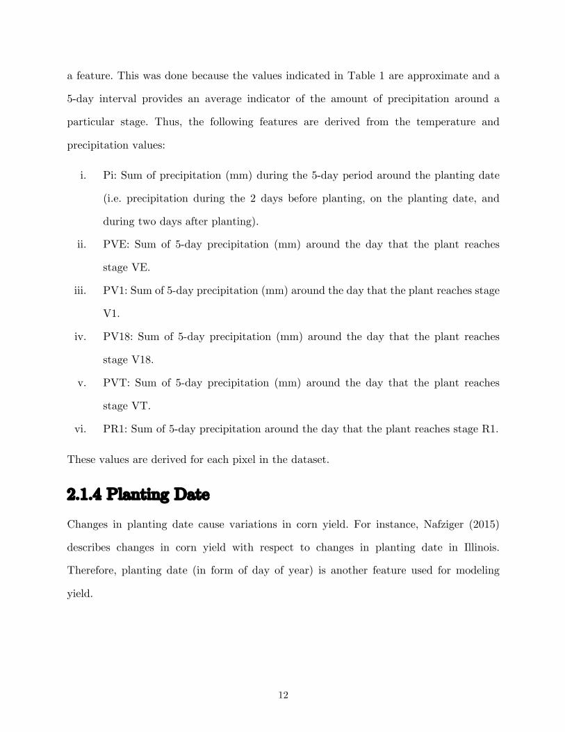
i.   Pi: Sum of precipitation (mm) during the 5-day period around the planting date

(i.e. precipitation during the 2 days before planting, on the planting date, and

during two days after planting).

ii.   PVE: Sum of 5-day precipitation (mm) around the day that the plant reaches

stage VE.

iii.   PV1: Sum of 5-day precipitation (mm) around the day that the plant reaches stage

V1.

iv.   PV18: Sum of 5-day precipitation (mm) around the day that the plant reaches

stage V18.

v.   PVT: Sum of 5-day precipitation (mm) around the day that the plant reaches

stage VT.

vi.   PR1: Sum of 5-day precipitation around the day that the plant reaches stage R1.

These values are derived for each pixel in the dataset.

2.1.4 Planting Date Changes in planting date cause variations in corn yield. For instance, Nafziger (2015)

describes changes in corn yield with respect to changes in planting date in Illinois.

Therefore, planting date (in form of day of year) is another feature used for modeling

yield.

  13

2.2 Machine Learning Models Because the outcome variable (i.e. yield) is known beforehand, supervised machine

learning models are used. This study uses two machine learning approaches: decision trees

and random forests. According to Hastie et al. (2009), decision trees "come closest to

meeting the requirements for serving as an off-the-shelf procedure for data mining" and

are scale invariant, robust to inclusion of irrelevant features and transformation of feature

values. However, they tend to have high variance and may overfit the training data.

Random Forests overcome this weakness and avoid overfitting by combining (“bagging”)

several decision trees (Breiman, 2001). More details on each approach are provided below.

2.2.1 Decision Trees A decision tree is a hierarchical model for supervised learning whereby a local prediction

region is identified in a sequence of recursive splits of the dataset (Alpaydin, 2010). It can

be used for both regression and classification. A decision tree consists of a number of nodes

that are used for recursive splitting of the data. Terminal nodes (nodes that have no

children) are also known as leaves. Each node represents a test applied to the input data

on whose basis the process follows one branch until it hits a leaf node. The leaf node

provides the outcome for the input.

The process of building a decision tree involves selecting a split that will lead to the

maximum decrease in variance (for a regression tree), which is identical to choosing the

split to maximize the between-groups sum-of-squares in a simple analysis of variance

(Therneau & Atkinson, 2015). Figure 5 below shows how a decision tree can be used for

regression.

  14

Figure 5: Example of a sample decision tree (maximum depth = 3) used for predicting corn yield. The dark nodes

represent predictions for the leaf nodes. The other nodes are represented in the form of a split condition. Data moves

to the right child if the condition evaluates to true and to the left if it evaluates to false.

An advantage of using decision trees is that their output is in a human-readable format.

However, a decision tree might lead to overfitting the training data because of noise in

the data. One way to overcome this problem is to limit the depth of the tree or pruning.

Alpaydin (2010) provides a detailed discussion on different ways of pruning. This study

uses the rpart R package (Therneau et al. 2015), which implements the algorithm

described by Breiman (1984) to build decision trees on the data.

After the tree is built on training data, it is then used to predict values of a testing dataset

that was not used for training. The accuracy of the model is then calculated using the

Root Mean Squared Error (RMSE) as defined in Equation 5.

𝑅𝑀𝑆𝐸 =   (_vN_9)wD9EF

Q (5)

where 𝑛 is the number of observations in the test set and 𝑦x and 𝑦; are the predicted and

actual label for the ith observation.

  15

The decision tree algorithm is also used to measure relative importance of different

variables. The importance is the reduction in variance from each variable used for splits.

For a detailed description of how variable importance is calculated in rpart, refer to

Therneau and Atkinson (2015).

2.2.2 Random Forests Random Forests are ensembles of several decision trees that have lower variance than

decision trees and hence reduce overfitting (Breiman, 1996). Bagging or bootstrap

aggregation is a technique is used to combine several decision trees into a random forest.

It refers to the process of combining several decision trees grown on different bootstrap

samples of the data. A bootstrap sample refers to a random sample of data with

replacement. Breiman (2001) describes the detailed algorithm for random forests that has

been used in this study. Breiman’s algorithm uses random features (variables) to construct

each tree (i.e., each tree is constructed on a different subset of features). One-third of the

total number of features were used for constructing each tree in the random forest. The

R package randomForest (Liaw & Wiener, 2002) was used to construct the random forest

in this study.

In random forests, cross-validation is not necessary to obtain a robust estimate of the

RMSE, because validation is done internally using OOB (out-of-bag) error estimation

(Breiman, 1996). Each tree is grown using two-thirds of the bootstrap sample of the

dataset. The remaining one-third of the data is used to evaluate the accuracy of the

learned model. The error estimate (mean squared error) on this one-third portion of the

data is called OOB error.

This method can also be used to calculate relative importance of different features. For

each tree, OOB error is measured in the form of mean squared error (MSE). The MSE is

  16

then measured again after permuting each predictor variable. The average normalized

difference between the two represents the importance of a variable. This turns out to be

useful for the purposes of this study, because the relative degree of influence of different

variables on yield can be quantified. In addition, this idea can be extended to calculate

the influence of each variable on corn yield for every observation by randomly changing

the value of the predictor variable (depending on the range of values) at every observation

point and measuring the mean squared error.

In addition, partial dependence plots, which give a graphical representation of marginal

effect of a variable on yield, can be drawn using this approach. Partial dependence of the

outcome on a variable is calculated using Equation 6:

𝑓 𝑥 =   yQ

𝑓(𝑥, 𝑥;z)Q;?y (6)

where 𝑥 is the variable for which partial dependence is sought, and 𝑥;z refers to the other

variables in the data. The summand refers to the model’s predicted value. The partial

dependence plot was used to plot the marginal effect on corn yield of different variables

such as slope, curvature, and precipitation.

 

  17

Chapter 3

Case Study This chapter presents a case study demonstrating the application and testing of the

methods discussed in the previous chapter.

3.1 Description of Data and Machine Learning

Models Corn yield data were obtained from 73 separate fields in northeastern Iowa distributed

over an area of approximately 5000 km2. The elevation in the region ranged from 244

meters to 364 meters. The study area had a gentle slope, the maximum value of which

was 8.6 degrees. Yield data were available in the form of a point dataset, where the value

of yield at each point represents the value of yield recorded by the harvesting equipment

at that point. The average spacing between a point and the nearest point in the dataset

is approximately 1.8 meters. This point dataset was used to obtain the yield raster as

described in chapter 2. Figure 6 shows the histogram of yield. Extreme values of yield

(yield greater than 400 and lower than 5) were removed from the dataset since these

values are highly unlikely to be observed and represent noise in the dataset.

  18

Figure 6: Histogram of yield values. It can be seen that yield ranges from 0 to 500 bushels/acre. Average yield is equal to approximately 166 bushels/acre.

Supervised machine learning techniques were used to build a model that predicts corn

yield based on the features and approaches described in Chapter 2.

Two machine learning models were used to model corn yield: decision trees and random

forests. The entire dataset was randomly shuffled and was divided into two parts: a

training set (containing 80% of the total data) and a test set (containing 20% of the total

data). Figure 7 shows the change in the cross-validation error as the maximum depth of

the decision tree is increased.

  19

Figure 7: 5-fold CV RMSE for decision tree of varying depths.

It can be seen from Figure 7 that the RMSE (Root Mean Square Error) of the decision

tree decreases with increase in the maximum depth. However, the rate of reduction of

error decreases. Thus, increasing depth indefinitely will not lead to a lower RMSE. In fact,

because the model uses a pruned decision tree, it is highly likely that the decision tree

algorithm would prune very deep branches. For example, the number of nodes in a

(pruned) decision tree of maximum depth 15 is 147 for this case study. This is significantly

different from the number of nodes in a comparable unpruned tree, which is 11,069. The

number of nodes in a decision tree of depth 14 is 145. Thus increasing the maximum depth

of a (pruned) decision tree does not change the structure of the tree significantly.

For the Random Forests model, 300 decision trees are aggregated (bootstrap aggregation)

to produce a better model (a model with a lower RMSE). Figure 8 shows the RMSE for

a random forest as the number of trees is increased.

  20

Figure 8: Change in RMSE for a random forest as the number of trees in the forest is increased.

It can be seen that as the number of trees increases, the random forest’s performance

improves. However, the RMSE undergoes very little reduction after the number of trees

reaches 200. In addition, as expected, the RMSE for random forest is lower than that of

the decision tree.

3.2 Results and Discussion

3.2.1 Comparison of Random Forest and Decision Tree Figure 9 shows the RMSE and correlation coefficient between actual and predicted yield

on the testing dataset (data that were not used in training at all) for both random forest

and decision tree models.

  21

Figure 9: Differences in performance of random forest and decision tree using (a) RMSE and (b) correlation coefficient

between actual and predicted yield.

Random forest has lower RMSE and higher correlation coefficient between actual and

predicted yield, demonstrating that aggregating several decision trees into a random forest

leads to better performance. Figures 10 and 11 show scatter plots of actual vs predicted

yield for decision tree (maximum depth = 15) and random forest.

Figure 10: Scatter plot of actual vs predicted yield for a decision tree (max. depth = 15).

  22

Figure 11: Scatter plot of actual vs predicted yield for a random forest (300 trees).

The scatterplots shown in Figures 10 and 11 indicate the robustness of a random forest

as compared to a decision tree. Certain bands of predictions can be seen in the scatterplot

for the decision tree because decision tree predictions are assigned in buckets (leaf nodes).

All observations falling in a particular leaf node are assigned the same value. Thus, the

predictions of the decision tree are more discretized.

However, the scatterplot for a random forest indicates more accurate estimates. The point

cloud is aligned closer to the 45o line as a result of the bootstrap aggregation of several

decision trees (300 in this case). This can be understood as averaging predictions of several

decision trees (i.e., Figure 11 having been derived by averaging several figures similar to

Figure 10).

3.2.2 Variable Importance Both decision trees and random forests can be used to rank variables (features) in order

of their importance in the model. This metric (variable importance) measures the relative

degree to which a feature variable influences corn yield. Figure 12 shows the relative

  23

variable importance for the best performing decision tree (maximum depth = 15) and

random forest (300 trees).

Figure 12: Relative Importance of different variables for (a) decision tree and (b) random forest.

Figure 12 displays significant differences in variable importance for decision trees and

random forests. For instance, TPI (Topographic Position Index) is the sixth most

important variable for the random forest model, whereas it is third from last for the

decision tree model. Apart from the differences in variable ranking are changes in

magnitude of importance of different variables.

For instance, in the case of the decision tree, the most important variable (planting date)

is more than twice as important as the next variable (Pi), whereas in the case of the

random forest, the change in magnitudes of importance is more gradual. This results from

the different ways in which variable importance is calculated, respectively, in decision tree

and random forest. As discussed in Chapter 2, each tree in a random forest is constructed

using a different subset of features (variables). This gives each variable a “chance” to

  24

increase its importance in the ranking. Because the random forest model has a lower

RMSE than the decision tree, the following discussion focuses only on the implications of

the importance of variables from the random forest.

Figure 12 (b) shows that “Plant Date” is the most significant variable influencing corn

yield. This shows that the choice of planting date could have a significant impact on corn

yield. However, planting date does not give much insight into factors influencing the

growth of a corn plant. “PVE”, “PV1” and “Pi” are the next three most important variables

after planting date. Thus, precipitation during the early stages of a corn plant’s growth

plays a major role in corn growth and hence yield. In addition, according to the random

forest model, precipitation during and around the reproduction stages (“PV18”, “PVT”,

and “PR1”) is less significant than during the early stages (PVE, PV1 and Pi).

Among topography-related features, TPI (Topographic Position Index), HAND (Height

Above Nearest Drainage), and slope are more important than TWI (Topographic Wetness

Index) and curvature, indicating that local topography (TPI) and local drainage potential

(HAND) have a significant impact on corn yield. However, soil type (percentage sand, silt

and clay) does not seem to have a significant impact on corn yield. The lesser importance

of soil-related variables can be attributed to the fact that the data comes from a similar

area with low variation in soil type.

However, comparing the importance of available water capacity in different layers of soil

gives interesting insights. Available water capacity in the 50–100mm deep segment of soil

is the most important compared to available water capacity at other depths (0-25mm, 25-

50mm and 100-150mm). Water capacity at this depth may affect uptake to the corn

plant’s roots water; the presence of moisture in this layer seems to be influencing yield

the most compared to water capacity at other depths.

  25

3.2.3 Partial Dependence While the previous section on relative importance of different variables gives useful insight

about factors affecting the growth of corn plants, the marginal distribution of different

feature variables over corn yield may be more helpful. Partial dependence plots (which

show the marginal distribution of a variable over corn yield) of six top variables from

Figure 12 summarize the influence of weather, topography and soil. The specific variables

are Planting Date, PVE, TPI, HAND, Slope and AWC_3, shown in Figures 13-18. Other

precipitation-related variables (with high relative importance)—Pi, PV1 and PR1—are

not analyzed since their relationship with yield is similar to that of PVE.

Figure 13: Partial dependence plot for planting date. The numbers on the x-axis indicate the day of year.

Figure 13 shows the partial dependence of yield on planting date. The plot shows how

yield changes for different planting dates. The top graph shows the number of observations

in the dataset for each planting date. It can be seen from the figure that earlier planting

dates have higher and more consistent yields than later planting dates. In addition, the

variation in yield increases as planting date is increased. A longer growing season leads to

a longer period for plants to absorb solar radiation, perform photosynthesis, and

  26

accumulate biomass and hence leads to higher yields (Kucharik, 2006). However, planting

early also has certain disadvantages: cold, wet soil that may produce a poor stand, more

difficult weed and insect control, and increased likelihood of frost damage after emergence

(Nafziger, 2015). According to Nafziger, 2015, “the advantages of early planting outweigh

the disadvantages.” This is in concurrence with our results for this dataset.

Next, the impact of precipitation on corn yield is analyzed, specifically the variable PVE

(sum of 5-day precipitation around the day the plant reaches stage VE). The plot below

shows the variation in yield as PVE is changed.

Figure 14: Partial dependence plot for PVE. The x-axis represents the sum of 5-day precipitation (mm) around the stage VE. The blue line represents a fitted curve (using loess method) on the data. The top plot shows the histogram

of PVE.

Figure 14 indicates an optimum range of precipitation that results in higher yields. As

PVE increases, yield initially increases; however, after reaching a maximum, yield

decreases again. This behavior can be attributed to waterlogging of plants from very high

precipitation.

  27

Next, impact of topography related feature variables on yield is analyzed. Figure 15 shows

the partial dependence of yield on TPI (Topographic Wetness Index).

Figure 15: Partial dependence plot of yield over TPI (Topographic Wetness Index). The top plot shows the histogram of TPI values.

Figure 15 shows the how yield changes with increase in TPI. Yield increases until TPI

reaches a value of approximately -1, after which it decreases again.

As described in the methods chapter, the TPI of a pixel is the difference in its elevation

with respect to nearby pixels. Thus, ridges would have a positive TPI, depressions would

have a negative TPI, and flat areas would have a TPI value close to zero. Figure 15 shows

that yield is highest in slight depressions and lower on ridges and deeper depressions,

which would influence the availability of water to the corn plant in regions with different

TPIs. Regions with very low TPIs are deep depressions, which might get waterlogged and

hence reduce yields. In contrast, regions with high TPIs are steep ridges whose high slope

may limit availability of water to corn plants. The areas with a slightly negative TPI

provide an ideal amount of water to the corn plant, and hence highest yield is observed

in these areas.

  28

Next, the changes in yield with respect to the Height Above Nearest Drainage (HAND)

are analyzed. Figure 16 shows the partial dependence plot of corn yield over HAND.

Figure 16: Partial dependence plot of yield over HAND (Height Above Nearest Drainage) (meters). The top plot shows the histogram of HAND values.

As in the case of the previous variables, an optimum range exists in which yield is highest

and deviations from this range lead to a decrease in corn yield. As Chapter 2 notes, HAND

is an indicator of local drainage potential. If this potential is too low, yield is very low, as

Figure 16 shows. As the drainage potential increases, yield also increases, reaching a

maximum beyond which a high drainage potential, leading to water draining quickly,

causes yield to decrease again.

Next, the relationship between slope and yield is analyzed. Figure 17 shows the partial

dependence plot of yield over slope.

  29

Figure 17: Partial dependence plot of yield over slope (degree). Top plot shows the histogram of slope values.

Like the other features, slope also shows a similar relationship with corn yield. An

optimum range of slope shows higher yields. Very flat and very steep areas lead to lower

yield.

The analysis of the topography-related features demonstrates that the interaction of

hydrology with topography significantly affects corn yield. Flat and steep areas lead to

lower yields when compared with regions in mild depressions. Mild depressions provide

an optimum amount of water to the plants, leading to higher yields.

Lastly, the most important soil-related variable (available water capacity of the segment

of soil with depth between 500 and 100 cm, or AWC_3) is analyzed. Figure 18 shows a

partial dependence plot of yield over AWC_3.

  30

Figure 18: Partial dependence plot of yield over AWC_3 (Available water capacity in a segment of soil of depth 50-100 cm in centimeters). The blue line shows a fitted curve (loess method). Top plot shows the histogram of AWC_3

values.

Figure 18 shows that yield is highest in the range of 25-28 cm for AWC_3 values. Very

low values of AWC_3 indicate low maximum moisture availability, which leads to a

reduction in corn yield. As the maximum moisture availability increases, yield also

increases.

Partial dependence plots can also be used to develop marginal plots of yield with respect

to two variables. Figure 19 shows the dependence plot of yield with respect to PVE and

TPI in the form of a heatmap.

  31

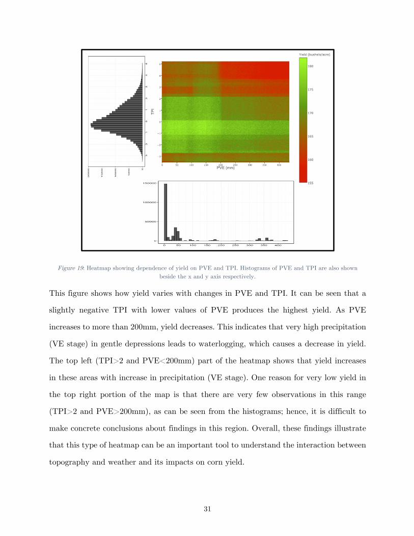
Figure 19: Heatmap showing dependence of yield on PVE and TPI. Histograms of PVE and TPI are also shown beside the x and y axis respectively.

This figure shows how yield varies with changes in PVE and TPI. It can be seen that a

slightly negative TPI with lower values of PVE produces the highest yield. As PVE

increases to more than 200mm, yield decreases. This indicates that very high precipitation

(VE stage) in gentle depressions leads to waterlogging, which causes a decrease in yield.

The top left (TPI>2 and PVE<200mm) part of the heatmap shows that yield increases

in these areas with increase in precipitation (VE stage). One reason for very low yield in

the top right portion of the map is that there are very few observations in this range

(TPI>2 and PVE>200mm), as can be seen from the histograms; hence, it is difficult to

make concrete conclusions about findings in this region. Overall, these findings illustrate

that this type of heatmap can be an important tool to understand the interaction between

topography and weather and its impacts on corn yield.

  32

A random forest model can also be used to draw field maps showing the importance of a

particular type of variable at the pixel level. This is done by randomly changing the value

of a variable (in the range of that variable) at a pixel and predicting yield. The higher the

error, the higher the importance of that variable at that pixel. To perform this analysis

efficiently, the features have been grouped into three types of variables:

i.   Topography: TPI, HAND, slope, TWI and curvature

ii.   Weather: Pi, PVE, PV1, PV18, PVT and PR1

iii.   Soil: AWC_1, AWC_2, AWC_3, AWC_4, sand (%), silt (%) and clay (%)

To demonstrate this technique, only one field has been analyzed; however, a similar

process can be applied to all of the fields.

Figure 20 shows the pixel-wise importance of soil related feature variables from the

perspective of the model (i.e., to what degree soil influences yield predictions at that

pixel). A value of 1 indicates that only soil influences yield at that pixel, and a value of 0

indicates that soil does not influence yield at all.

Figure 20: Pixel-wise importance of soil related features (AWC_1, AWC_2, AWC_3, AWC_4, sand (%), silt (%), clay (%)).

  33

From Figure 20 it is apparent that soil is not the main predictor of yield in a field, since

most of the pixels are either red or yellow (which signifies low pixel importance). This is

because soil type varies very little within a field.

Figure 21 shows the pixel-wise importance of the same field for weather-related variables,

which affect yield more than soil-related variables.

Figure 21: Pixel-wise importance of weather related features (PVE, PV1, PV18, PVT, PR1).

Clusters of “green” areas in the figure indicate that weather influences yield to a moderate

degree. Most of these clusters are either on ridges (high TPI) or valleys (low TPI). This

shows that precipitation plays a major role in influencing yield in regions with very low

and very high TPI. Regions with low TPI would get waterlogged and regions with high

TPI would get drained fairly quickly and hence the amount of precipitation will influence

corn yield significantly.

Lastly, the impact of topography-related variables on yield in the same field is considered.

  34

Figure 22: Pixel-wise importance of topography related features (TPI, TWI, HAND, Slope and curvature).

Figure 22 indicates that topography plays the dominant role in influencing yield within a

field, more than soil- or weather-related variables. The dominance of topography most

strongly influences corn yield in most ridges and valleys. Thus, topography along with

precipitation are the dominating variables (influencing yield) in these regions.

These maps could be used to delineate a farm into localized micro-management zones

based on which variable(s) dominate(s) yield, and management decisions could then focus

only on the dominating variables. For instance, micro-regions where precipitation is the

dominating factor (e.g., slopes in water-scarce areas), will be the ones requiring the most

irrigation.

  35

Chapter 4

Discussion and Conclusions This study has demonstrated how machine learning applied to fine-grained yield, weather,

topography, and soil data can provide insights on the small-scale processes affecting yield.

Decision tree and its ensemble (random forest) were used for their simplicity, ease of

application, and powerful predictive capabilities. The accuracy obtained in this study

(correlation = 0.78) is similar to that obtained by Pantazi et al. (2016) (classification

accuracy of 78 to 82 percent for different methods). However, Pantazi et al. (2016) used

experimental data from only one field and predicted classes of yield (low, medium and

high) instead of the actual value of yield.

This study used large-scale yield data (276,262 observations at 10-meter scale) collected

from farm equipment (combines) during routine operations in 73 corn fields to test the

benefits of a “Big Data” approach to understanding yield and its hydrologic influences. In

contrast, previous studies have relied mostly on imagery data or experimental observations

from a small number of points. Using a large dataset obtained from actual fields at high

resolution has several advantages. First, in contrast to experimental fields (which are

generally located in a very small geographical region), such datasets would have higher

diversity in topography, soil, and precipitation patterns if they could be collected from

numerous fields. Furthermore, data obtained from actual fields may provide better

representation of conditions prevailing in the real world as compared to an experimental

field. Second, in contrast to datasets which are spread over large areas but have coarser

  36

resolution, this dataset can be used to study yield variability both within a field and across

different fields.

A case study with data from Iowa showed that planting date, precipitation during the

initial stages of corn growth, and topographic position index (TPI) were the most

significant variables in predicting yield. Partial dependence plots generated by the random

forest model describe the marginal distribution of corn yield over different variables and

help in understanding how yield changes with respect to different variables. Corn yield

was highest in depressions with gentle slope, an indicator of how the interaction of

hydrology and topography affects corn yield. Depressions with gentle slope provide

sufficient water to the plant without waterlogging and hence produce higher yields.

However, a 2-d partial dependence plot in the form of a heatmap (yield vs TPI and PVE)

showed that corn yield decreases in depressions with gentle slope if precipitation (VE

stage) is very high, which is an indicator of waterlogging in these areas. In contrast, ridges

showed a slight increase in corn yield upon increase in precipitation (VE stage). However,

it was difficult to conclude anything about ridges with very high precipitation due to

limited number of observations in the training data.

Additionally, intra-field maps showed further detail on the importance of different types

of variables and can be used to delineate fine-grained management zones in a field. This

is a promising direction for future research to explore.

This study has a few limitations. First, the weather and yield data came from a single

year (i.e., 2013). The model would likely be able to predict yield more accurately if weather

and yield data from multiple years were used to train the model.

Further, the accuracy of the predictive model is reduced if it is used to predict yield in

fields that were not in the training dataset. The testing set used in this study was created

  37

by selecting a proportion (20 percent) of the randomly shuffled dataset. This means that

some of a corn field’s observations are used in the training set and the rest in the testing

set. When the model was to be used to predict corn yield on fields completely different

from the training set (i.e., an external set of fields whose observations were not part of

the training set), accuracy of model predictions declined significantly. For instance, the

RMSE of a random forest (500 trees) on an external set of fields was 35.4 bushels/acre

(32 percent increase) and the correlation was 0.52.

Additionally, the fields used in this study were all from the same region in Iowa, providing

little inter-field variation in weather- and soil-related variables. Additional data from other

locations would be needed to generalize the model and improve its applicability to more

diverse conditions.

Finally, information regarding fertilizer application was not available. Fertilizers could

have a major role in influencing yield, and inclusion of fertilizer-related feature variables

could improve the predictive model.

  38

References 1.   Alpaydin, E. (2010). Introduction to Machine Learning. The MIT Press.

2.   Ayoubi, S., & Sahrawat, K. L. (2011). Comparing multivariate regression and artificial

neural network to predict barley production from soil characteristics in northern Iran.

Archives of Agronomy and Soil Science, 57(5), 549-565.

3.   Ayoubi, S., Khormali, F., & Sahrawat, K. L. (2009). Relationships of barley biomass and

grain yields to soil properties within a field in the arid region: use of factor analysis. Acta

Agriculturae Scandinavica, Section B — Soil & Plant Science, 59(2), 107-117.

4.   Beven, K., & Kirby, M. (1979, March). A physically based, variable contributing area

model of basin hydrology. Hydrological Sciencis Bulletin, 24(1).

5.   Breiman, L. (n.d.). Out of bag estimation. Retrieved November 1, 2015, from Statistics

Department, University of California, Berkeley:

https://www.stat.berkeley.edu/~breiman/OOBestimation.pdf

6.   Carter, J., Schmid, K., Waters, K., Betzhold, L., Hadley, B., Mataosky, R., & Halleran,

J. (2012, November). Lidar 101: An Introduction to Lidar Technology Data, and

Applications. Retrieved from NOAA Coastal Services Center:

https://coast.noaa.gov/digitalcoast/_/pdf/lidar101.pdf

7.   Cassel, D. K., & Nielsen, D. R. (1986). Field capacity and available water capacity.

Methods of Soil Analysis: Part 1—Physical and Mineralogical Methods, 901-926.

8.   De Reu, J., Bourgeois, J., Bats, M., Zwertvaegher, M., & Gelorini, A. (2013).

Application of the topographic position index to heterogeneous landscapes.

Geomorphology, 186, 39-49.

  39

9.   Dilts, T. E. (2015). Topography tools for ArcGIS 10.1. Retrieved February 12, 2016,

from http://www.arcgis.com/home/item.html?id=b13b3b40fa3c43d4a23a1a09c5fe96b9

10.  Environmental Systems Research Institute. (2014). ArcGIS Desktop: Release 10.

Redlands, California.

11.  GeoInformatics Training Research Education and Extension (GeoTREE) Center,

University of Northern Iowa. (n.d.). Iowa Lidar Mapping Project. Retrieved September

2014, from GeoTREE: http://www.geotree.uni.edu/lidar/

12.  Grabs, T., Siebert, J., Bishop, K., & Laudon, H. (2009). Modeling spatial patterns of

saturated areas: A comparison of the topographic wetness index and a dynamic

distributed model. Journal of Hydrology, 373(1), 15-23.

13.  Kravchenko, A. N., & Bullock, D. G. (2000). Correlation of corn and soybean grain yield

with topography and soil properties. Agronomy Journal, 92(1), 75-83.

14.  Kucharik, C. J. (2006). A multidecadal trend of earlier corn planting in the central USA.

Agronomy Journal, 98(6), 1544-1550.

15.  Liaw, A., & Wiener, M. (2002). Classification and Regression by randomForest. R News,

2(3), 18-22.

16.  Mutanga, O., Elhadi, A., & Moses, A. C. (2012). High density biomass estimation for

wetland vegetation using WorldView-2 imagery and random forest regression algorithm.

International Journal of Applied Earth Observation and Geoinformation, 18, 399-406.

17.  Nafziger, E. (n.d.). Corn. Retrieved June 2, 2015, from Extension & Outreach, Crop

Sciences Department, College of ACES, University of Illinois:

http://extension.cropsciences.illinois.edu/handbook/pdfs/chapter02.pdf

18.  Nobre, A. D., Cuartas, L. A., Hodnett, M., Renno, C. D., & Rodrigues, G. (2011).

Height Above the Nearest Drainage–a hydrologically relevant new terrain model. Journal

of Hydrology, 404(1), 13-29.

  40

19.  Norouzi, M., S, A., Jalalian, A., Khademi, H., & Dehghani, A. A. (2010). Predicting

rainfed wheat quality and quantity by artificial neural network using terrain and soil

characteristics. Acta Agriculturae Scandinavica, Section B — Soil & Plant Science,

60(4), 341-342.

20.  Pantazi, X. E., Moshou, D., Alexandridis, T., Whetton, R. L., & Mouazen, A. M. (2016).

Wheat yield prediction using machine learning and advanced sensing techniques.

Computers and Electronics in Agriculture, 121, 57-65.

21.  PRISM Climate Group, O. S. (2004, February 4). Retrieved from

http://prism.oregonstate.edu

22.  Remote Sensing Division, National Geodetic Survey. (n.d.). Light Detection and Ranging

(LIDAR). Retrieved October 10, 2014, from National Geodetic Survey, National Oceanic

and Atmospheric Administration:

http://www.ngs.noaa.gov/RESEARCH/RSD/main/lidar/lidar.shtml

23.  Soil Survey Staff, Natural Resources Conservation Service, United States Department of

Agriculture. Soil Survey Geographic (SSURGO) Database. Available online at

http://websoilsurvey.nrcs.usda.gov/. Accessed July/2015.

24.  Therneau, T. M., & Atkinson, E. J. (2015, June 29). An Introduction to Recursive

Partitioning Using the RPART Routines. Retrieved from https://cran.r-

project.org/web/packages/rpart/vignettes/longintro.pdf

25.  Therneau, T., Atkinson, B., & Ripley, B. (2015). rpart: Recursive Partitioning and

Regression Trees. Retrieved from http://CRAN.R-project.org/package=rpart

26.  Waheed, T., Bonnell, R. B., Prasher, S. O., & Paulet, E. (2006). Measuring performance

in precision agriculture: CART—A decision tree approach. Agricultural water

management, 84(1), 173-185.

  41

27.  White, A. B. (2005). Vegetation Variability and Its Hydro-Climatologic Dependence.

Universit of Illinois, Civil and Environmental Engineering.